INTERNATIONAL JOURNAL OF CLIMATOLOGY, VOL. 14, 287-305 (1994) 551.526.6(267):55 1.577.2 l(94):55 1.5 13.7

INDIAN OCEAN SEA-SURFACE TEMPERATURE PATTERNS AND AUSTRALIAN WINTER RAINFALL

IAN SMITH

Centre for Drought Research, CSIRO Division of Atmospheric Research. P B I , Mordialloc, Victoria, 3195, Australiu

Received 25 August 1992 Accepted 6 April 1993

ABSTRACT

Indian Ocean sea-surface temperatures (SSTs) for the period 1950-1988 are analysed using principal component analysis, and their relationships with Australian winter rainfall totals for the period 1950-1979 are studied using regression analysis. As has been demonstrated by others, significant simultaneous correlations exist between the dominant patterns in the Indian Ocean and the wintertime rainfall over a large part of Australia. There is also evidence of significant correlations between autumn SST patterns and winter rainfall.

These relationships are tested using multiple linear-regression-based predictions of winter rainfall categories for the period 1980-1988. Skill is quantified in terms of categorical predictions. Predictions based on the autumn SSTs exhibit more skill than those based on the autumn SOI, but much less than predictions based on the concurrent winter indices.

KEY WORDS Sea-surface temperatures Principal component analysis Australian rainfall Predictability Skill Multiple Linear Regression

INTRODUCTION

A number of studies have revealed correlations between various indices of the Southern Oscillation and seasonal district rainfall over the Australian continent. The strongest correlations are generally found over northern and south-eastem Australia during spring (September-November), with the weakest correlations occurring during autumn (March-April). Correlations are generally weak over the western third of the continent (McBride and Nicholls, 1983; Drosdowsky and Williams, 1991). These correlations have, until recently, formed the basis of the seasonal outlooks issued by the Bureau of Meteorology (National Climate Centre, 1988), which utilize lag correlations between the Southern Oscillation Index (SOI) and rainfall totals for various districts. The SOI, representing the sea-level pressure gradient across the Pacific, is a useful, convenient index which measures just one aspect of fluctuations of the atmosphere-ocean system. Allan et al. (1990) have shown that northern Australian sea-levels exhibit significant correlations with Australian district rainfall during winter and spring and that these correlations are at least as strong as those between rainfall and either SO1 or northern Australian sea-surface temperatures (SSTs). These relationships indicate that sea- level anomalies provide another useful index, which may reflect the combined effects of barometric and wind forcings on the seasonal time-scale, particularly those associated with ENS0 events. Monitoring of sea-levels in near real time is expected to provide additional skill to seasonal rainfall predictions. Global SSTs can now also be monitored and analysed in near real time. Parker et al. (1988) and Ward and Folland (1991) have demonstrated how statistical seasonal rainfall predictions for the Sahel region and northern Brazil can be made using the strength of SST patterns in the Atlantic and Pacific Oceans. Based on the results of several previous studies, similar predictions for much of Australia may be feasible using SST patterns in the Indian and Pacific Oceans.

Simmonds (1990) provides a summary of a number of studies that have dealt with SST-Australian rainfall relationships. Of these, Whetton (1990) used principal component (PC) analysis on 11 years of monthly SST

CCC 0899-841 8/94/030287-19 0 1994 by the Royal Meteorological Society

288 I. SMITH

data from 159 grid points covering the eastern Indian and western Pacific Oceans around Australia. The resultant patterns showed some correlation with Victorian (south-eastern Australia) rainfall patterns but the results were not encouraging as far as seasonal forecasting is concerned.

Nicholls (1989) used rotated PC analysis on Australian wintertime rainfall data for the period 1946-1979 and isolated two major patterns. The first of these (PCP1) was strongly correlated (coefficient = 0.75) with an SST gradient in the Indian Ocean, whereas the second (PCP2) was correlated (0.55) with the Southern Oscillation Index (SOT). The correlation pattern between PCPl and SSTs revealed a dipole structure with centres over Indonesia and the central Indian Ocean, which was still evident when the partial correlation with the SO1 was taken into account. Both Simmonds (1990) and Frederiksen et al. (1990) have studied the effect of idealized warm SST anomalies near Australia and successfully simulated enhanced precipitation and circulation changes in association with anomalies to the north and west-a result consistent with the observations but whose interpretation is not straightforward. Simmonds et al. (1992) show that similar precipitation changes can be simulated if a surface pressure anomaly, similar to that accompanying the SST anomaly, is prescribed in the absence of SST anomalies.

Nicholls (1989) also suggested that some predictability of winter rainfall was possible given the persistence of the SST anomalies. Further studies by Drosdowsky (1993a) identified teleconnections between a PCP1- type pattern (denoted as T6) and both mean sea-level pressure and wind fields. Drosdowsky (1993b) noted that the SST and wind patterns showed signs of development as early as March, which further indicated possibilities for prediction. The major question addressed in this paper concerns the strength of the Indian Ocean SST and winter rainfall relationship and how this translates into useful predictive skill. This is investigated by considering relationships between winter rainfall and the March-April-May (MAM) and June- July-August (JJA) SST patterns. This approach differs from Nicholls (1989), who related rainfall PCs to SSTs and the SOI, but is similar to that of Ward and Folland (1991), whereby principal component patterns (or unrotated covariance eigenvectors) of SSTs are calculated for individual oceans for individual seasons. The strength of these patterns is related to the SOT, Australian wintertime rainfall indices PCPl and PCP2, and individual Australian district seasonal rainfall totals. These relationships are then tested through regression analysis. Multiple linear regression fits to seasonal data for the period 1950-1979 are used to predict rainfall totals for the subsequent years 1980-1988, and these are assessed using categorical skill scores. The relationships between Australian rainfall and Pacific Ocean SST patterns are described elsewhere, as these represent a purely ENS0 phenomenon. The aim here is to investigate an apparently independent phenomenon involving just the Indian Ocean SSTs.

DATA

The time series of both the MAM and JJA SO1 over the period of interest is shown in Figure 1. Warm- and cold-event years according to Kiladis and Diaz (1989) are indicated on the time series. It should be noted that these identified years are based on both the behaviour of the SOT and an SST anomaly index for the eastern equatorial Pacific. A year is classified as year 0 of an event (as in Rasmusson and Carpenter (1982)) if the SOT changed sign (positive to negative for warm events and vice versa) and Pacific SST anomalies became established. Only the first year of multiyear events are considered. It can be seen that there are some events that are not associated with extreme values for the SO1 (e.g. 1954, 1957, 1969, 1970) while extreme values for the SOT do not always coincide with identified events (e.g. 1950, 1955, 1977).

The SSTs used in this study come from the Global Ocean Surface Temperature Atlas (GOSTA) described by Bottomley et al. (1990). A global coverage is provided by GOSTA on a 5" by 5" grid and is characterized by a high standard of quality control. There is a good standard of coverage from 1950 onwards, but in data- sparse regions values have been generated by interpolation of surrounding values and preserving the structure present in the long-term climatological data of Alexander and Mobley (1976) (see Bottomley et al. (1990) for details). Monthly values from January 1950 through to December 1988 were averaged to provide seasonal averages. Rainfall data for Australia from the National Climate Centre, Bureau of Meteorology comprise district monthly totals over the same period which were also combined into seasonal averages.

INDIAN OCEAN SST AND AUSTRALIAN WINTER RAIN 289

-10

15

wcw wcw c C W I , , I , , , , , I w wc w

-25 1 1 1 ' " " " " ~ ' ' 1 1 1 1 1

1950 1953 1956 1959 1962 1965 1968 1971 1974 1977 1980 1983 1986 1989

Figure I . Time series of the MAM SO1 (dashed) and JJA SO1 (solid) 1950-1988. Warm- and cold-event years are indicated

The Indian Ocean basin is defined by the boundaries 40"E to 140"E and 50"s to 25"N. These boundaries include points representing the South China, Philippine, and Arafura seas and therefore our definition of the Indian Ocean basin is not precise but serves to describe the majority of the points involved. From within the above boundaries, the 5" data were averaged to 10" grid boxes with the aim of providing a reasonable spatial sample without overburdening the analysis procedure. Ward and Folland (1991) noted that the use of 10" resolution data provided a satisfactory spatial resolution. No grid points were used if the averaging procedure encountered missing (i.e. land) values. As a result, 68 points were used to define the SST patterns for the Indian Ocean (see Figure 2). It should be noted that observations were relatively sparse in the central Indian Ocean during the 1950s.

Principal component analysis (see Richman, 1986) was performed separately on the data for both the autumn and winter seasons. The principal component patterns (PCPs) for each season (representing the

30N

0

lr4 u o 0 0 0 0 0 1 I

0 0 0 0 0 0 0 0 0 0 0 I I I

30E 6OE 90E 120E

Figure 2. Central locations of the 10" grid boxes used for principal component analysis of the SST data

290 I. SMITH

unrotated eigenvectors of the covariance matrix of the detrended SSTs), together with the amplitude time series, were then analysed. Detrending removes the effects of long-term changes in SST that are present in the data and which can interfere with the analysis of decadal and interannual fluctuations (e.g. Ward and Folland, 199 1). The resultant patterns, by definition, explain the maximum variance with the least number of components. This is desirable for the purposes of establishing concise multiple linear regression (MLR) relationships between the pattern strengths and other variables. Rotation of the patterns may help to better identify important regional patterns but this is not regarded as necessary for this type of statistical study.

SST PATTERNS

Figure 3 shows the first five PCPs (Al-A5) for the autumn (MAM) season together with their associated amplitude time series. The percentage variance associated with the first seven PCPs is shown in Figure 4. The first three account for over 50 per cent and are distinct from the remainder. This is illustrated by the associated

0

305

1: I,, I , , I , , I , , , , , I , , , , , I , , I , , , , , , , , , 1 , I ,j -9

- 10 1950 1953 1956 1959 1962 1965 1968 1971 1974 1977 1980 1963 1986 1989

Figure 3. (a-e) The first five principal component patterns and associated amplitude time series for Indian Ocean MAM SSTs (1950-1988)

INDIAN OCEAN SST AND AUSTRALIAN WINTER RAIN

-8

-9

29 1

-

-

I I . . I I I 30E 6OE 9oE 120E

sampling errors calculated according to the criterion of North et al. (1982). (For a sample size of N , the sampling error is given by (2/N)"'. Because N=39 here, the sampling error is plus or minus 23 per cent.) Principal component pattern A1 is characterized by a south-west to north-east gradient which peaked during 1965 and has decreased in amplitude over recent time. The A2 pattern is characterized by a south-west to north-east dipole pattern south of the Equator, whereas A3 is characterized by a relatively strong centre west of Australia. Table I shows that the latter pattern is correlated moderately (r =0*36) with the MAM SO1 (for a sample size of 39, the correlation coefficient r is significant at the 95 per cent level if it exceeds 0.32).

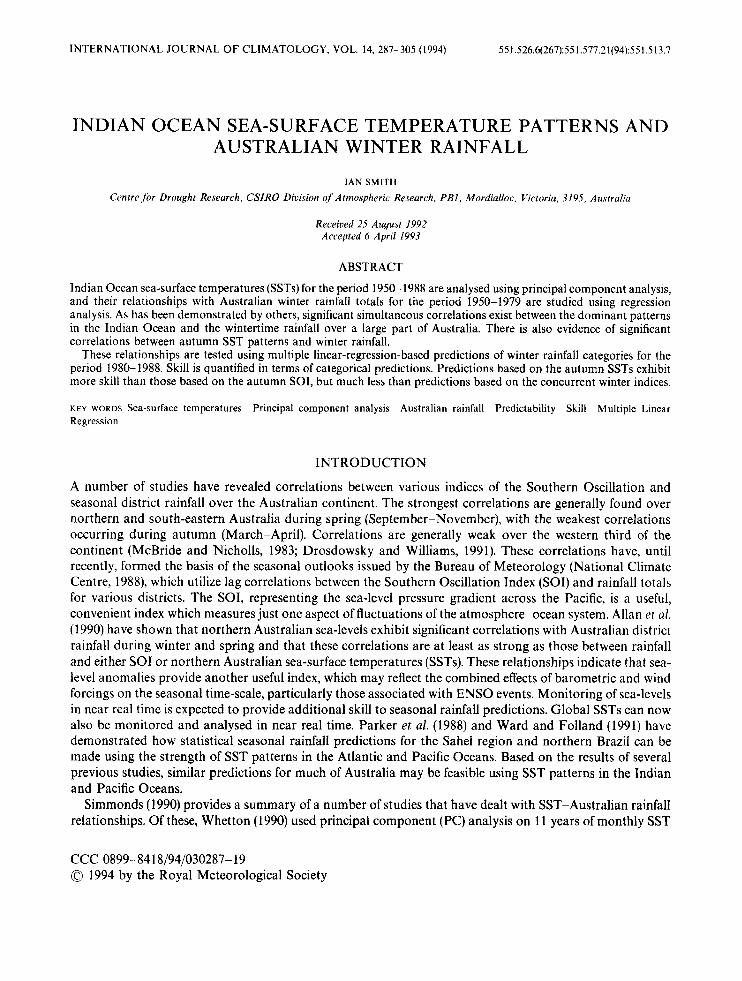
Figure 5 shows the first five PCP patterns (Jl-J5) for the winter (JJA) season. Figure 6 shows the distri- bution of variance amongst the first seven PCPs, but in this case none of the leading components stand out as distinct from the remainder. Pattern J1 is similar to its autumn counterpart A1 and, as Table I indicates, their amplitude time series are correlated significantly (r=0.50) (r is significant at the 99 per cent level if it exceeds 0-42). Pattern 52 is also dominated by a south-west to north-east structure and is correlated significantly with A2 ( r = 0.46). Pattern 53 is similar to A3, both in terms of structure and amplitude (r = 057).

292 1. SMITH

I C I I I 30E 6oE 9 E 120E

5 t i 4 -

3 2 -

1 -

0 ,

1 --

It is also correlated significantly with the JJA SO1 (r =0.55). Pattern 54 is related to both A2 (r = 0.46) and A4 (r=O.47), but there is no evidence of any reiationship between J5 and any other pattern or index. There is also no evidence of significant relationships involving the remaining patterns beyond A5 and J5. On this basis we retain just the first five patterns in each case and assume that the remainder represent noise in the data. It is likely that the fifth patterns also contain no useful information and may tend to make the results of regression analyses more conservative than otherwise.

RELATIONSHIPS WITH RAINFALL PATTERNS

The two major Australian winter rainfall components found by Nicholls (1989) are referred to as PCPl and PCP2 and are based on data for the period 1950- 1979. PCP1, which accounts for over 30 per cent of the total variance represents a north-west to south-east type pattern and is weakly related to the SOI. Pattern PCP2, which accounts for about 25 per cent of the total variance, and represents an east-west type pattern is strongly

INDIAN OCEAN SST AND AUSTRALIAN WINTER RAIN 293

t I * I I I 30E 6CE 9oE 1 ZOE

-a -10 !i -9 II-,,,Ii

1950 1953 1956 1959 1962 1965 1968 1971 1974 1977 1980 1983 1986 1989

Figure 3d.

related to the SOL The correlation between the strength of these patterns and each of the autumn and winter SST patterns is shown in Table 11. (In these cases the sample size is 30 and r is significant at the 99 per cent level if it exceeds 0.46.) Pattern PCPl is correlated most strongly (r=0.69) with 52, whereas PCP2, the ENSO- related pattern, is not correlated significantly with any of the patterns (including the remaining patterns in each case). Importantly, J2 is very similar to both the pattern of correlation between SSTs and PCPl found by Nicholls (1989) and that between SSTs and the rainfall pattern T6 found by Drosdowsky (1993a).

Confirmation of the above relationships is provided by MLR fits to both PCPl and PCP2 using the first five SST components as independent variables. (In this case the MLR coefficient r is significant at the 99 per cent level if it exceeds 049). Table I1 shows that a linear combination of the winter SST components can explain a large fraction of the variance associated with PCPl ( I =0.70), much more than that associated with PCP2 (r = 0.48). The autumn SSTs in combination also appear to be correlated significantly with PCPl (r=0.55) but less so with PCP2 (r=0.48). These results not only confirm the existence of a simultaneous

294 1. SMITH

I I . I I

3G€ 6oE 9oE t ME

ti 1, , I , , I , , I , I I , , I , , I , , I , , I , , I , , I , , I , , I , ,I -9

-10 1950 1953 1956 1959 1962 1965 1968 1971 1974 1977 1980 1983 1986 1989

Figure 3e.

relationship between the winter rainfall pattern and Indian Ocean SSTs, but also indicate that some predictability may be evident in the relationship with autumn SSTs. There is less evidence for predictability of the ENSO-related pattern PCP2.

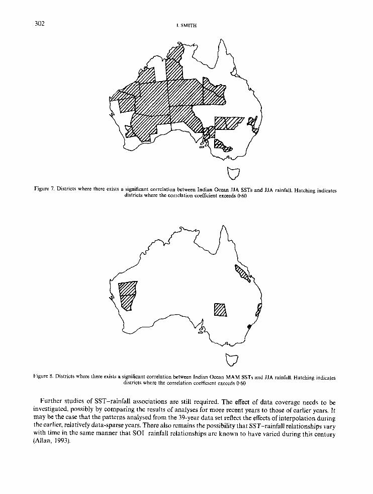
Figure 7 shows a map of those districts where significant correlations occur between the five winter SST components and the winter rainfall totals for the period 1950-1979. Only those districts where r exceeds 0.60 are shown. As expected, these reveal a pattern similar to PCP1, i.e. dominated mainly by a north-west to south-east structure, but also suggestive of the PCP2-ENSO-type structure as indicated by districts in eastern Australia and along the east coast.

Figure 8 shows the same map based on the autumn SSTs and the winter rainfall totals. There are far fewer districts where r exceeds 060. There is obviously a much weaker resemblence to PCP1, but there is also some indication of the presence of the PCP2-ENSO-type structure evident in the previous figure. The problem is to test whether these relationships indicate useful predictability.

INDIAN OCEAN SST AND AUSTRALIAN WINTER RAIN 295

1 2 3 4 5 6 7

Figure 4. Percentage variance associated with the first seven principal components for Indian Ocean MAM SSTs

Table I. Correlations between the MAM SST patterns Al-A5, the JJA SST patterns Jl-J5, and SO1 for MAM and JJA

MAM JJA J1 52 33 54 J5 so1 so1

A1 A2 A3 A4 A5 J 1 52 53 54 J5

0.50 028 0.29 0.21 0.3 1 0.24 0.49 0.46 0.29 0.46 000 0.16 0.12 0.33 057 0.23 0.13 0.36

0.47 0.03 0.18 007 0.10

0.14 0.27 0.55 0.08 0.19

0.04 0.10 0.19 0.12 0.27 007 0.35 0.25 0.35 0.13

METHODS OF TESTING FOR PREDICTABILITY

Testing can be performed by using the MLR relationships for each district based on the 'calibration' period 1950-1979 and verifying the resultant predictions for the subsequent period 1980-1988. Ward and Folland (199 1) discuss a number of methods and difficulties associated with assessing rainfall predictions. Assessments can be made of the predicted rainfall amount, the predicted most likely rainfall category, or the predicted probabilities of the rainfall falling within predefined categories (linear discriminant analysis).

Figure 9 illustrates a difficulty with regression-based predictions of rainfall. It shows an example of predictions of raw winter rainfall amounts for a district in north Queensland compared to observations. The total number is 39 and, although they are based on linear regression, the predictors used are irrelevent-they simply serve to provide the example. It can be seen that the distribution of the predictions and observations is very different and this contributes to a relatively low correlation coefficient of 0.21. The predictions are biased away from extreme events and tend to be clustered about the mean (the predicted totals lie within the range 13-34 mm whereas the observations lie within the range 5-130 mm). One method which avoids these problems is to consider the success at predicting rainfall categories rather than raw rainfall totals. This can be done by ranking the fitted values and the observations independently so that, in the long term, the predicted categories have the same distribution as the observed categories-an important prerequisite for defining random prediction skill levels (see Livezy, 1987). The categories adopted by the Bureau of Meteorology are

296 1. SMITH

I C I I

30E 60E 90E 120E

1950 1953 1956 1959 1962 1965 ]YE8 i971 1974 1977 1980 1983 1986 1989

Figure 5. (a-e) The first five principal component patterns and associated amplitude time series for Indian Ocean JJA SSTs (1950-1988)

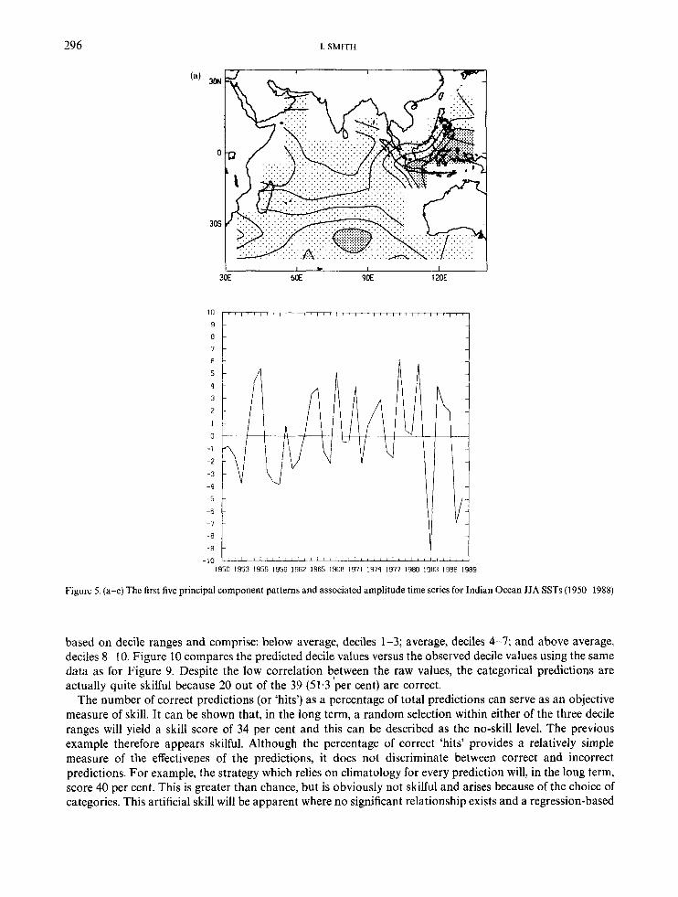
based on decile ranges and comprise: below average, deciles 1-3; average, deciles 4-7; and above average, deciles 8- 10. Figure 10 compares the predicted decile values versus the observed decile values using the same data as for Figure 9. Despite the low correlation between the raw values, the categorical predictions are actually quite skilful because 20 out of the 39 (51.3 per cent) are correct.

The number of correct predictions (or 'hits') as a percentage of total predictions can serve as an objective measure of skill. It can be shown that, in the long term, a random selection within either of the three decile ranges will yield a skill score of 34 per cent and this can be described as the no-skill level. The previous example therefore appears skilful. Although the percentage of correct 'hits' provides a relatively simple measure of the effectivenes of the predictions, it does not discriminate between correct and incorrect predictions. For example, the strategy which relies on climatology for every prediction will, in the long term, score 40 per cent. This is greater than chance, but is obviously not skilful and arises because of the choice of categories. This artificial skill will be apparent where no significant relationship exists and a regression-based

INDIAN OCEAN SST A N D AUSTRALIAN WINTER RAIN 297

I I I I I 30E 60E 9oE 1 ME

I I L I I l _ U L I I L 1 L L L L J-LLI 1LJ

1: 1, , 1 1 , , / , -10

1350 1953 1956 1959 1962 1965 196R 1371 1974 1377 1380 1383 1986 1989

Figure 5b.

relationship always yields values clustered about the mean. This can be avoided by constructing a contingency table that penalizes incorrect predictions. Gandin and Murphy (1992) describe a method of formulating equitable skill scores that discriminate between true and artificial skill. Table I11 shows one possible scoring matrix associated with the three decile ranges used here. The positive scores are inversely proportional to the probabilities associated with each category whereas the negative weightings are such that a random selection of categories will, in the long term, yield a score of zero. This is true also of any of the simple strategies that adopt average, below average, or above average conditions each time. In the long term a perfect set of N predictions will score 3 N . Summing the weighted results and scaling by 100/3N yields a weighted skill score that usually has values in the range between near 0 per cent (no skill) and 100 per cent (perfect skill). Slightly negative scores can sometimes be expected but substantially negative scores would imply negative skill. Such cases rarely arise. Both the weighted scores and the percentage ‘hits’ score can provide an alternative measure of the relationships suggested by the correlation coefficients. In the example

298 I. SMITH

L I C I I

30E 60E 9 E 1 ME

7

6

5

4 3

2

1

0

- I

-2

-3

-4

-8

- I 0 -9 i 1950 1953 1956 1959 1962 1965 1968 1971 1974 1977 1980 1983 1986 1989

Figure 5c.

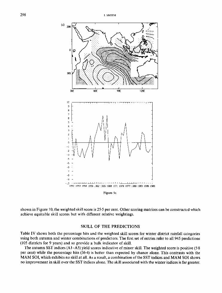
shown in Figure 10, the weighted skill score is 25.5 per cent. Other scoring matrices can be constructed which achieve equitable skill scores but with different relative weightings.

SKILL OF THE PREDICTIONS

Table IV shows both the percentage hits and the weighted skill scores for winter district rainfall categories using both autumn and winter combinations of predictors. The first set of entries refer to all 945 predictions (105 districts for 9 years) and so provide a bulk indicator of skill.

The autumn SST indices (Al-AS) yield scores indicative of minor skill. The weighted score is positive (5.8 per cent) while the percentage hits (36-4) is better than expected by chance alone. This contrasts with the MAM SOI, which exhibits no skill at all. As a result, a combination of the SST indices and MAM SO1 shows no improvement in skill over the SST indices alone. The skill associated with the winter indices is far greater.

lNDIAN OCEAN SST AND AUSTRALIAN WINTER RAIN 299

(dl 3m

0

30s

I . 1 I I 6oE 9oE 120E

5 i

Figure 5d.

Both the SST indices and the JJA SO1 exhibit skill separately, as they do in combination (17.6 per cent and 43.8 per cent).

These results are indicative, but include results from all the districts irrespective of whether the MLR relationships are significant or not. The second set of entries refers to stratified data and comprises subsets of eight districts where the correlations from the calibration period are most significant. These districts are the same as those shown in Figure 8. For each set of predictors, only those with the highest correlations are used. Again it can be seen that the autumn SST indices, unlike the MAM SOI, provide positive, albeit minor predictive skill. Whether these relationships are in fact useful for these districts remains questionable as the skill is not high and the winter rainfall totals for these regions are not as important as for districts further south.

The stratified results for the winter indices reveal that the highest skill levels (22.9 per cent and 45.8 per cent) can be achieved by combining the SST indices and the JJA SOI, but that most of the skill is due to the SSTs.

300 1. SMITH

3oN

0

30s

I I t I I I 30E 6oE 9oE 1 ME

_;I,,l , , , , , , ( , l , , , i , , , , , I ( , , , , , , 1 -9

-10 L L L U L .

1950 1953 1956 1959 1962 1965 1968 1971 1974 1977 1980 1983 1986 19E9

Figure 5e.

This difference with the unstratified results suggests that a strong correlation between the JJA SO1 and rainfall does not always lead to high predictive skill. The reverse is also implied, i.e. that high predictive skill is sometimes associated with a low correlation. One possible reason for this result is that, unlike the SST association, the JJA SOT-rainfall association may vary in time. The eight districts where skill is evident are shown in Figure 11. In this case the relationships appear useful because they refer to districts in South Australia where winter rainfall is important. On the other hand, the relationships are simultaneous and would be useful only if the SSTs could be predicted in advance.

DISCUSSION

The results of principal component analyses of seasonal SSTs and regression analyses have illustrated the strong simultaneous correlations between Indian Ocean SSTs and Australian winter rainfall found by

INDIAN OCEAN SST AND AUSTRALIAN WINTER RAIN 301

25 1 1 1 2 3 4 5 6

20 I - c

1 2 3 4 5 6 7

Figure 6. Percentage variance associated with the first seven principal components for Indian Ocean JJA SSTs

Table 11. Correlations between the Australian winter rainfall patterns PCPl and PCP2 (1950-1979) and: the MAM SST patterns (both individually and in linear combination); the JJA

SST patterns (ditto); and the SO1 for MAM and JJA ~~

PCPl PCP2

A1 A2 A3 A4 A5 A1 + A2 f A3 + A4 -i- A5 J1 52 53 54 55 J1 + J2 + 53 + 54 + J5 MAM SO1 JJA SO1

0.04 0.21 0.20 0.26 045 055 0.03 069 026 004 0.12 070 0.05 0.28

~~

0.30 003 0.30 018 0.1 1 0.48 012 0.01 0.27 0.27 0.14 0.48 038 0.55

Nicholls ( 1 989) and Drosdowsky (1993a). However, despite these simultaneous correlations, testing of categorical predictions on 9 years of independent data reveals only minor skill associated with the autumn SSTs as predictors. Furthermore, any apparent skill does not appear to be particularly useful.

The question as to the whether the SST anomalies cause the rainfall anomalies or simply reflect changes in the atmospheric circulation has often been raised (e.g. Flohn, 1986; Nicholls, 1989; Simmonds, 1990; Whetton, 1990; Simmonds et al., 1992). A recent study by Drosdowsky (1993b) suggests that summertime wind anomalies may force the SST anomalies, which then persist through to winter. The general circulation model results of Simmonds et al. (1992), in which positive wintertime rainfall anomalies over Australia can be simulated given the imposition of an anomalous low pressure centre to the north-west of Australia, suggest that SST anomalies in the same region do not provide a direct thermal forcing through evaporation anomalies, but instead act indirectly by assisting the maintenance of anomalous low-level circulations. Both these studies imply that indices of anomalous circulation features early in the year may provide more predictive skill than the SST anomalies themselves.

302 1. SMITH

W

Figure 7. Districts where there exists a significant correlation between Indian Ocean JJA SSTs and JJA rainfall. Hatching indicates districts where the correlation coefficient exceeds 0.60

Figure 8. Districts where there exists a significant correlation between Indian Ocean MAM SSTs and JJA rainfall. Hatching indicates districts where the correlation coefficient exceeds 060

Further studies of SST-rainfall associations are still required. The effect of data coverage needs to be investigated, possibly by comparing the results of analyses for more recent years to those of earlier ycars. It may be the case that the patterns analysed from the 39-year data set reflect the effects of interpolation during the earlier, relatively data-sparse years. There also remains the possibility that SST-rainfall relationships vary with time in the same manner that SOI-rainfall relationships are known to have varied during this century (Allan, 1993).

INDIAN OCEAN SST AND AUSTRALIAN WINTER RAIN

140 +

120 - s 2: 100 - 2 n

E E 60 -

cu != 40 -

Q)

0 80 - v

- - . .c .- Ki ;* .

* * * \ * . . * . a: 20 - : :I*-**

0,

303

c

t

10

9

1

0

Deciles (predicted)

Figure 10. The same data as in Figure 9 but expressed in terms of decile ranges

Table 111. Weightings associated with categorical predictions of be- low average (decile range 1-3), average (decile range 4-7) and above

average (decile range 8-10) conditions

Below Above average Average average

Below average 3.33 - 1.67 - 1.1 1

Above average -1.11 - 1.67 3.33 Average - 1.67 2.50 - 1.67

304 1. SMITH

Table IV. Assessments of Australian district winter rainfall predictions (1 980-1988)

Predictors Weighted score Percentage ‘hits’

A t , A2, A3, A4, A5 MAM SO1 A l , A2, A3, A4, AS, MAM SO1 J1, J2, 53, J4, J5 JJA SO1 J1, J2, 53, 54, J5, JJA SO1

Stratified Al , A2, A3, A4, AS MAM SO1 Al , A2, A3, A4, AS, MAM SO1 J1, J2, J3, J4, J5 JJA SO1 Jl ,J2, J3,J4, J5, JJA SO1

5.8

6.0 17.0 19.5 17.6

-0.14

8.3 - 3.0

3.2 19.5 4.4

22.9

36.4 32.6 36.6 42.8 45.6 43.8

38.2 30.5 35.5 43.2 34.7 45.8

b Figure 11. The eight districts where multiple linear regression yields the highest correlations between a combination of J l , J2,33,34, 5 5

and JJA SO1 and JJA rainfall

ACKNOWLEDGEMENTS

This work was supported by the Land and Water Resources Research and Development Council (now incorporating the Australian Water Research Advisory Council). The author would like to thank Harvey Davies and Tony Davies for providing software support, and Drs Robert Allan, Barrie Hunt, and Peter Whetton for many helpful comments. Thanks are also extended to two anonymous referees whose suggestions considerably improved an earlier version of this paper.

REFERENCES

Alexander, R. C. and Mobley, R. L. 1976. ‘Monthly average sea-surface, temperatures and ice-pack limits on a 1 deg. global grid’, Mon. Wen. Rea., 107, 896-910.

INDIAN OCEAN SST AND AUSTRALIAN WINTER RAIN 305

Allan, R. J., Beck, K. and Mitchell, W. M. 1990. ‘Sea level and rainfall correlations in Australia: tropical links’, J . Climate, 3, 838-846. Allan, R. J. 1993. ‘Historical fluctuations in ENSO and teleconnection structure since 1879: near global patterns’, Quaternary Australasia,

Bottomley, M., Folland, C. K., Hsiung, J., Newell, R. E., and Parker, D. E. 1990. Global Ocean Surface Temperature Atlas (GOSTA), Joint Meteorological Office/Massachusetts Institute of Technology Project, US Department of Energy, US National Science Foundation, and US Office of Naval Research, and UK Departments of Energy and Environment, HMSO, London, 20 pp and 313 plates.

Drosdowsky, W. 1993a. ‘An analysis of Australian seasonal rainfall anomalies: 1950-1987. 11: temporal variability and teleconnection patterns’, Int. J . Climatol., 13, 1-30.

Drosdowsky, W. 1993b. ‘A method of forecasting winter rainfall over southern and eastern Australia’, Aus. Meteorol. Mag., 42, 1-6. Drosdowsky, W. and Williams, M. 1991. ‘The Southern Oscillation in the Australian region. Part 1: anomalies at the extremes of the

Flohn, H. 1986. ‘Indonesian droughts and their teleconnections’, Berliner Geogr. Stud., 20, 251-265. Frederiksen, C. S., Drosdowsky, W., Balgovind, R. C., and Nicholls, N. 1990. ‘Indian Ocean sea surface temperatures and Australian

Gandin, L. S. and Murphy, A. H. 1992. ‘Equitable skill scores for categorical forecasts’, Mon. Wen. Rev., 120, 361-370. Kiladis, G. N. and Diaz, H. 1989. ‘Global climatic anomalies associated with extremes in the southern oscillation’, J . Climate. 2,

Livezy, R. E. 1987. ‘The evaluation of skill in climate predictions’, in: Radok, U. (ed.) Toward Understanding Climate Change, Westview

McBride, J. L. and Nicholls, N. 1983. ‘Seasonal relationships between Australian rainfall and the Southern Oscillation’, Mon. Wen. Rev.,

National Climate Centre 1988. Seasonal Outlooks (Based on El Niiio/Southern Oscillation (ENSO) Relationships), Bureau of

Nicholls, N. 1989. ‘Sea surface temperatures and Australian winter rainfall’, J . Climate, 2, 965-973. North, G . R., Bell, T. L., Cahalan, R. F. and Moeng, F. J. 1982. ‘Sampling errors in the estimation ofempirical orthogonal functions’, Mon.

Parker, D. E., Folland, C. K. and Ward, M. N. 1988. ‘Sea surface temperature anomaly patterns and prediction of seasonal rainfall in the

Richman, M. B. 1986. ‘Rotation of principal components’, J . Climate, 6, 293-335. Rasmusson, E. M. and Carpenter, T. H. 1982. ‘Variations in tropical sea surface temperature and surface wind fields associated with the

Simmonds, I. 1990. ‘A modelling study of winter circulation and precipitation anomalies associated with Australian region ocean

Simmonds, I. H., Rocha, A. and Walland, D. 1992. ‘Consequences of winter tropical pressure anomalies in the Australian region’, Int. J .

Ward, N. M. and Folland, C. K. 1991. ‘Prediction of seasonal rainfall in the north Nordeste of Brazil using eigenvectors of sea-surface

Whetton, P. H. 1990. ‘Relationships between monthly anomalies of Australian region sea-surface temperature and Victorian rainfall’,

11, 17-27.

oscillation’, J . Climate, 4, 619-638.

rainfall’, Int. TOGA Con$ Proc., WCRP-43, 229-239.

1069-1090.

Press, Boulder and London, 200 pp.

11, 1998-2004.

Meteorology, Melbourne.

Wea. Rev., 110, 699-706.

Sahel region of Africa’, in Gregory, S . (ed.), Recent Climatic Change, Bellhaven, London, pp. 166-178.

Southern Oscillation/El Nifio’, Mon. Wea. Rev., 110, 354-384.

temperatures’, Aus. Meteorol. Mag., 38(3), 151-162.

Climatol., 12, 419-434.

temperature’, Int. J. Climatol., 11, 71 1-743.

Aus. Meteorol. Mag., 38, 17-41.