Indian Institute of Technology KanpurDepartment of Electrical Engineering

B.Tech. Project Report (EE 492)

Finite Element Modelling of Radiation Conditionsin Electromagnetic Scattering

Vivek Saxena (Y6549)viveks@iitk.ac.in

Advisor: Dr. Naren NaikDepartment of Electrical Engineering

IIT Kanpur

Second Semester (2009-10)

Contents

Contents 2

Certificate 3

Abstract 4

Acknowledgments 5

List of Figures 6

1 Introduction 7

2 Motivation & Objectives 9

3 Literature Survey 10

4 Work Done in the Final Semester 11

5 Basic Theory 125.1 Scattering Boundary Value Problem . . . . . . . . . . . . . . . . . . . . . . . . . . . 12

5.1.1 Scalar Problem . . . . . . . . . . . . . . . . . . . . . . . . . . . . . . . . . . 125.1.2 Vector Problem . . . . . . . . . . . . . . . . . . . . . . . . . . . . . . . . . . 13

5.2 The Finite Element Method . . . . . . . . . . . . . . . . . . . . . . . . . . . . . . . 145.3 Meshing . . . . . . . . . . . . . . . . . . . . . . . . . . . . . . . . . . . . . . . . . . 15

5.3.1 Concentric Ring Meshing for circular objects . . . . . . . . . . . . . . . . . . 155.3.2 DistMesh . . . . . . . . . . . . . . . . . . . . . . . . . . . . . . . . . . . . . 175.3.3 COMSOL-based Meshing . . . . . . . . . . . . . . . . . . . . . . . . . . . . . 19

5.4 Mesh Truncation . . . . . . . . . . . . . . . . . . . . . . . . . . . . . . . . . . . . . 20

6 Methodology Adopted 256.1 Statement of the Forward Problem (for Cylindrical PEC Object in Air) . . . . . . . 26

6.1.1 The Partial Differential Equation for the Total Electric Field . . . . . . . . . 266.2 Statement of the Forward Problem (for Buried Mines) . . . . . . . . . . . . . . . . . 27

6.2.1 Parameter Values . . . . . . . . . . . . . . . . . . . . . . . . . . . . . . . . . 28

1

7 Results 297.1 Circular PEC Object centered at the origin . . . . . . . . . . . . . . . . . . . . . . . 297.2 Location of 2nd order ABC vs. that of 1st order ABC . . . . . . . . . . . . . . . . . 317.3 Circular PEC Object placed off center . . . . . . . . . . . . . . . . . . . . . . . . . 327.4 Concave PEC Object . . . . . . . . . . . . . . . . . . . . . . . . . . . . . . . . . . . 337.5 Square PEC Object placed off center . . . . . . . . . . . . . . . . . . . . . . . . . . 347.6 Two PEC Objects . . . . . . . . . . . . . . . . . . . . . . . . . . . . . . . . . . . . . 357.7 Comparison between 1st order ABC and PML PEC Cylinder in Air . . . . . . . . . 367.8 Comparison between ABC and PML for Dielectric Cylinder in Air . . . . . . . . . . 377.9 The Subsurface Problem (Half Space Scattering) . . . . . . . . . . . . . . . . . . . . 387.10 PEC Cylinder buried under Soil . . . . . . . . . . . . . . . . . . . . . . . . . . . . . 387.11 Dielectric Cylinder buried under Soil . . . . . . . . . . . . . . . . . . . . . . . . . . 397.12 Scattering from a PEC Cylinder in Air using the First Order ABC (Effect of varying

Discretization) . . . . . . . . . . . . . . . . . . . . . . . . . . . . . . . . . . . . . . . 40

8 Conclusions 41

References 42

Appendix A: Finite Element Method Formulation 43Weak Form . . . . . . . . . . . . . . . . . . . . . . . . . . . . . . . . . . . . . . . . . . . 45Element Matrices and Vectors . . . . . . . . . . . . . . . . . . . . . . . . . . . . . . . . . 46Integration over an arbitrary triangular patch . . . . . . . . . . . . . . . . . . . . . . . . 47Enforcement of Dirichlet Conditions . . . . . . . . . . . . . . . . . . . . . . . . . . . . . . 48Assembly of Matrix Elements . . . . . . . . . . . . . . . . . . . . . . . . . . . . . . . . . 48Solution of the Linear System . . . . . . . . . . . . . . . . . . . . . . . . . . . . . . . . . 49

Appendix B: First Order Absorbing Boundary Condition 50

Appendix C: Second Order Absorbing Boundary Condition 52

Appendix D: COMSOL Results 59

Appendix E: MATLAB Codes for Meshing 2D Regions 638.1 Meshing Code for Cylinder . . . . . . . . . . . . . . . . . . . . . . . . . . . . . . . . 638.2 Meshing Code for Off-center Cylinder . . . . . . . . . . . . . . . . . . . . . . . . . . 658.3 Meshing Code for Square Object . . . . . . . . . . . . . . . . . . . . . . . . . . . . 658.4 Meshing Code for Concave Object . . . . . . . . . . . . . . . . . . . . . . . . . . . . 668.5 Meshing Code for Two Objects . . . . . . . . . . . . . . . . . . . . . . . . . . . . . 67

Appendix F: MATLAB FEM Codes 698.6 First Order ABC . . . . . . . . . . . . . . . . . . . . . . . . . . . . . . . . . . . . . 698.7 Second Order ABC . . . . . . . . . . . . . . . . . . . . . . . . . . . . . . . . . . . . 77

2

Certificate

This is to certify that the work contained in this report entitled “Finite Element Modelling of Ra-diation Conditions in Electromagnetic Scattering” by Vivek Saxena has been carried out under mysupervision and that this work has not been submitted elsewhere for a degree or diploma.

Dr. Naren NaikDepartment of Electrical EngineeringIIT Kanpur

3

Abstract

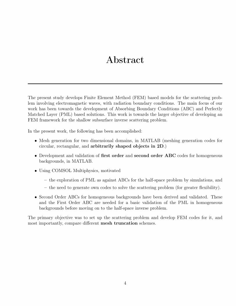
The present study develops Finite Element Method (FEM) based models for the scattering prob-lem involving electromagnetic waves, with radiation boundary conditions. The main focus of ourwork has been towards the development of Absorbing Boundary Conditions (ABC) and PerfectlyMatched Layer (PML) based solutions. This work is towards the larger objective of developing anFEM framework for the shallow subsurface inverse scattering problem.

In the present work, the following has been accomplished:

• Mesh generation for two dimensional domains, in MATLAB (meshing generation codes forcircular, rectangular, and arbitrarily shaped objects in 2D.)

• Development and validation of first order and second order ABC codes for homogeneousbackgrounds, in MATLAB.

• Using COMSOL Multiphysics, motivated

– the exploration of PML as against ABCs for the half-space problem by simulations, and

– the need to generate own codes to solve the scattering problem (for greater flexibility).

• Second Order ABCs for homogeneous backgrounds have been derived and validated. Theseand the First Order ABC are needed for a basic validation of the PML in homogeneousbackgrounds before moving on to the half-space inverse problem.

The primary objective was to set up the scattering problem and develop FEM codes for it, andmost importantly, compare different mesh truncation schemes.

4

Acknowledgments

I thank my advisor, Dr. Naren Naik, for his support and encouragement throughout the academicyear, and for introducing me to the finite element method, subsurface scattering, and other existingacademic issues and problems arising in computational electrodynamics.

Vivek SaxenaRoll Number: Y6549Fourth Year UndergraduateB.Tech. ProgrammeDepartment of Electrical EngineeringIIT Kanpurviveks@iitk.ac.in

5

List of Figures

1.1 Basic geometry of a Landmine Detection Problem . . . . . . . . . . . . . . . . . . . 71.2 Block Diagram of the Forward Scattering Problem . . . . . . . . . . . . . . . . . . . 81.3 Block Diagram of the Inverse Scattering Problem . . . . . . . . . . . . . . . . . . . 8

5.1 Flowchart of the Finite Element Method-based solution process . . . . . . . . . . . 145.2 Triangular Mesh Pattern for h = 0.09 . . . . . . . . . . . . . . . . . . . . . . . . . . 165.3 Set Theoretic Operations on Regions . . . . . . . . . . . . . . . . . . . . . . . . . . 185.4 Circular Mesh generated using DistMesh . . . . . . . . . . . . . . . . . . . . . . . . 195.5 Mesh for a Concave PEC Object . . . . . . . . . . . . . . . . . . . . . . . . . . . . 205.6 The unbounded and PML-bounded problems . . . . . . . . . . . . . . . . . . . . . . 225.7 The three step-process for setting up a PML . . . . . . . . . . . . . . . . . . . . . . 23

7.1 First and Second Order Solutions for PEC Cylinder Scattering . . . . . . . . . . . . 297.2 Analytical and FEM Solutions for the PEC Cylindrical Scatterer at λ/25 . . . . . . 307.3 1st order ABC versus 2nd order ABC . . . . . . . . . . . . . . . . . . . . . . . . . . 317.4 Electric Fields near an off-center PEC Cylinder . . . . . . . . . . . . . . . . . . . . 327.5 Scattering from an off-center PEC Cylinder . . . . . . . . . . . . . . . . . . . . . . 327.6 Electric Fields near a Concave PEC Object . . . . . . . . . . . . . . . . . . . . . . . 337.7 Scattering from a Concave PEC Object . . . . . . . . . . . . . . . . . . . . . . . . . 337.8 Square PEC Object Mesh . . . . . . . . . . . . . . . . . . . . . . . . . . . . . . . . 347.9 Scattering from a Square PEC Object . . . . . . . . . . . . . . . . . . . . . . . . . . 347.10 Mesh for two PEC objects . . . . . . . . . . . . . . . . . . . . . . . . . . . . . . . . 357.11 Scattering from Two PEC Objects . . . . . . . . . . . . . . . . . . . . . . . . . . . . 357.12 Scattered Fields from PEC Cylinder in Air: ABC vs PML . . . . . . . . . . . . . . 367.13 Scattering from Dielectric Cylinder in Air: ABC vs PML . . . . . . . . . . . . . . . 377.14 Scattering from PEC Cylinder buried under Soil . . . . . . . . . . . . . . . . . . . . 387.15 Scattering from Dielectric Cylinder buried under Soil . . . . . . . . . . . . . . . . . 39

8.1 FEM Local Node Numbering Convention . . . . . . . . . . . . . . . . . . . . . . . . 448.2 Evaluation of ABC matrix elements . . . . . . . . . . . . . . . . . . . . . . . . . . . 518.3 Scattered Fields from PEC Cylinder in Air: ABC vs PML . . . . . . . . . . . . . . 598.4 Scattering from Dielectric Cylinder in Air: ABC vs PML . . . . . . . . . . . . . . . 608.5 Scattering from PEC Cylinder buried under Soil . . . . . . . . . . . . . . . . . . . . 618.6 Scattering from Dielectric Cylinder buried under Soil . . . . . . . . . . . . . . . . . 62

6

Chapter 1

Introduction

Subsurface imaging is the reconstruction of topological attributes of an object buried underneathor embedded within the volume of a dielectric material. It involves the use of data of the elec-tromagnetic fields scattered by the object(s) of interest, to construct a contour map of the totalelectromagnetic field distribution in the near region of the scatterer(s). From this contour map andthe field data, it is usually possible to recover important details of the structure, using reconstruc-tion algorithms.

Important examples of subsurface imaging are landmine detection, tumor detection, geophysicaland oil exploration. The basic problem is conveyed effectively by the following illustration:

Figure 1.1: Basic geometry of a Landmine Detection Problem

The figure shows a spherical/cylindrical mine (shown in red) buried underneath the ground (soil,shown in maroon), which is in general undulating. The mine is the object of interest here and thequantities of relevance in this problem can be:

• the depth below surface, of the mine, and• the structure of the mine.

These quantities can quantify the extent of destruction an explosion of the mine could cause. Thedepth can be used to determine whether the mine can be safely defused without risking an explo-sion, and the structural (material) content can give hints for identifying it so as to enable the useof specifically practical methods to defuse it.

An analogous situation arises in biomedical imaging, where structural information about a tu-mor or an abnormal growth in the body can be used to advance prognosis, possibly allowing early

7

detection and improving the chances of patient treatment and survival in the case of a malignanttumor. In this problem, the “mine” of the Figure 1.1 is replaced by a possibly malevolent growthinside the body, and the interface becomes the skin-air interface. It is extremely important that themethods of imaging be non-invasive; that is, the process of recovery of compositional informationmust not result in perturbation which causes damage or destruction. For instance, tumors cannotbe imaged using ionizing radiation which might cause them to grow in size or become malignant.Of course, landmines should not be touched more if one can help it.

Subsurface imaging problems form actually a subset of a larger category of problems known asInverse Problems. In general, to predict the results of a measurement requires

1. a model of the system under investigation, and,2. a physical theory linking the parameters of the model to the parameters being measured.

This prediction of observations (in our case, the scattered fields), given the values of the parametersdefining the model (object topology, dielectric properties) constitutes the forward problem.

Figure 1.2: Block Diagram of the Forward Scattering Problem

Solving the inverse problem consists of using the results of actual observations (the scattered fields)to infer the values of the parameters characterizing the system under investigation (the shapedescriptors of the mine and its depth below the surface).

Figure 1.3: Block Diagram of the Inverse Scattering Problem

8

Chapter 2

Motivation & Objectives

Subsurface imaging is the non-invasive recovery of shape and topological attributes of an objectburied within a dielectric region, for example, a mine buried beneath the soil. The method of imag-ing referred to here involves propagating electromagnetic waves of known frequency and amplitudeon the ground, measuring the fields scattered by the dielectric surface (soil) and the object (mine),and estimating the internal electromagnetic parameters of the scatterer.

In both landmine detection as well as tumor detection, there are several practical issues to consider,namely

• Need for a non-invasive detection.

• Low False Alarm Rate.

• Distinguishing between landmines and clutter, or malignant and benign tumors.

For such purposes, tomographic reconstruction of the subsurface object is essential. And as moti-vated earlier, subsurface reconstruction is an inverse scattering problem.

The objective of this project is towards the development of a computational model for study-ing and analyzing subsurface imaging of objects buried under the soil, using the Finite ElementMethod. Towards this objective, this study investigates the use of Absorbing Boundary Conditionsand Perfectly Matched Layers to model the radiation conditions at infinity.

Inverse scattering solutions typically need forward scattering models. Specifically, it is desirableto have complete control over the implementation aspects of the forward problem model, for in-stance the FEM routines and the boundary conditions, because these are used to generate Frechetderivatives required for shape reconstruction. Hence, writing our own code for solving the forwardproblem through FEM is preferred over usage of existing forward problem solvers such as COM-SOL Multiphysics. However, the power of these packages cannot be undermined, and ideally it isdesirable to use both approaches to solve the complete problem.

9

Chapter 3

Literature Survey

The first part of the project involved familiarization with the Finite Element Method (FEM),through the reading of the textbooks by Jin [1], Polycarpou [2] and Volakis et al [4], to understandhow Maxwell’s equations are discretized into linear matrix equations. This discretization procedureis described in Appendix A. For meshing, before setting up our own triangular meshing codes,the documentation of DistMesh [3], an open source MATLAB-based meshing library, was studied.DistMesh is used here in conjunction with our own meshing codes, to specify objects which havesigned distance function descriptions, as described in section 5.3.2 of this report.

Next, a study of the two dimensional boundary value problem described by Polycarpou [2] andJin [1] and the three major boundary conditions (Dirichlet, Neumann and Mixed Boundary Con-ditions) was undertaken. The weak form was developed using these ideas, and the mathematicalfoundations underlying them, as outlined by Volakis et al [4] and Kesavan [5]. The Galerkin for-mulation of Jin [1] was identified to be used for subsequent computational work, and a Helmoltzequation was set up for a general two dimensional scattering problem. This is described in Chapter5, of this report.

Existing literature on Abvsorbing Boundary Conditions (ABCs) by Bayliss et al [6], Volakis andChatterjee [9] and on the Perfectly Matched Layers (PMLs) by Johnson [8], Bérenger [10], Rappa-port and Winton [11], and Jin and Chew [12], was studied. For the 1st and 2nd order ABCs, thetreatments of Jin [1] and Volakis et al [4] were examined and taken up for implementation to solvea prototypal scattering problem of scattering from a PEC cylinder. This was motivated by theexistence of an analytical solution for the total and scattered fields, as given by Balanis [7], and byresults for the 1st order ABC given by Polycarpou [2]. Certain mistakes in Jin’s formulation of the2nd order ABC expressions were discovered, as outlined in Appendix C. Experiments with the PMLwere conducted in COMSOL Multiphysics, an FEM Modelling package. Simulation results aregiven in Chapter 6, and analytical expressions for the ABC are given in Appendices B and C.

For more complicated 2D objects which cannot be described easily using explicit signed distancefunctions, a MATLAB program was written to interface with COMSOL’s meshing subroutines.For this purpose, the documentation of COMSOL was studied to gain access to the internal meshstorage structure. Both COMSOL’s meshing subroutines as well as those of DistMesh had to beaugmented with our own interface codes to make the meshes compatible with the FEM codes.

10

Chapter 4

Work Done in the Final Semester

• Development of completely general 2D nodal FEM codes to handle arbitrary two dimensionalobjects.

• Development of a framework to mesh arbitrary two dimensional objects.

• Derivation and validation of the Second Order Absorbing Boundary Condition (ABC) expres-sions in homogeneous backgrounds, in an FEM model.

• Study of comparison between First Order and Second Order ABCs, for various 2D objects,including a double object scattering example.

• Validation of the superiority of the Second Order ABC over the First Order ABC for theobjects considered, and a brief study of the limitations of the second order ABC.

• Development of interface codes to use MATLAB in conjunction with DistMesh (an open sourcelibrary of geometric primitives and meshes) and COMSOL Multiphysics (a commercial FEMmodeling package, used this semester solely for meshing complex objects).

Work Done in the First Semester• Familiarization with the 2D Nodal Finite Element Method and methods of mesh truncation

(ABC and Perfectly Matched Layers ).

• Development of a framework to mesh circular and rectangular objects.

• Development of codes to solve Laplace and Poisson equations in 2D for electrostatic problems,and extension of the code to solve the Helmoltz equation in 2D.

• Derivation and validation of the First Absorbing Boundary Condition (ABC) expressions inhomogeneous backgrounds, in an FEM model.

• Development of a program to solve for the total and scattered electric fields in the vicinity ofa PEC cylinder in air, using the FEM and a First Order ABC for mesh truncation.

• Study of comparison between First Order ABC and PML via COMSOL Multiphysics (usedas an FEM Modeling package).

• Validation of the improved performance of the PML over the First Order ABC for subsurfacescattering, through COMSOL Multiphysics.

11

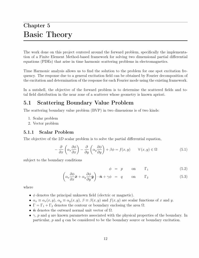
Chapter 5

Basic Theory

The work done on this project centered around the forward problem, specifically the implementa-tion of a Finite Element Method-based framework for solving two dimensional partial differentialequations (PDEs) that arise in time harmonic scattering problems in electromagnetics.

Time Harmonic analysis allows us to find the solution to the problem for one spot excitation fre-quency. The response due to a general excitation field can be obtained by Fourier decomposition ofthe excitation and determination of the response for each Fourier mode using the existing framework.

In a nutshell, the objective of the forward problem is to determine the scattered fields and to-tal field distribution in the near zone of a scatterer whose geometry is known apriori.

5.1 Scattering Boundary Value ProblemThe scattering boundary value problem (BVP) in two dimensions is of two kinds:

1. Scalar problem2. Vector problem

5.1.1 Scalar ProblemThe objective of the 2D scalar problem is to solve the partial differential equation,

− ∂

∂x

(αx∂φ

∂x

)− ∂

∂y

(αy∂φ

∂y

)+ βφ = f(x, y) ∀ (x, y) ∈ Ω (5.1)

subject to the boundary conditions

φ = p on Γ1 (5.2)(αx∂φ

∂xx+ αy

∂φ

∂yy

)· n+ γφ = q on Γ2 (5.3)

where

• φ denotes the principal unknown field (electric or magnetic).• αx ≡ αx(x, y), αy ≡ αy(x, y), β ≡ β(x, y) and f(x, y) are scalar functions of x and y.• Γ = Γ1 + Γ2 denotes the contour or boundary enclosing the area Ω.• n denotes the outward normal unit vector of Ω.• γ, p and q are known parameters associated with the physical properties of the boundary. In

particular, p and q can be considered to be the boundary source or boundary excitation.

12

Boundary condition (4.1) is known as the Dirichlet condition, whereas boundary condition (4.2) isknown as the Robin condition or the generalized Neumann boundary condition.

For an open domain scattering problem, the appropriate boundary condition on the far field isthe Sommerfeld Radiation condition [1]

limr→∞

r

[∇×

(EH

)+ jk0r ×

(EH

)]= 0 (5.4)

which in two dimensions becomes

limρ→∞

√ρ

[∂

∂ρ

(EzHz

)+ jk0

(EzHz

)]= 0 (5.5)

where ρ =√x2 + y2, r =

√ρ2 + z2 and k0 is the free space propagation wavenumber.

But for a numerical solution to this BVP, we cannot store information for ρ → ∞ on a com-puter with finite memory size. The Sommerfeld Radiation condition as expressed in the form aboveis no longer valid, since the domain has to be truncated by some artificial boundary that is locateda finite distance away from the scatterer.

Hence, we need to enforce a suitable boundary condition on this artificial boundary such thata perfect absorbing surface is simulated. By the use of an artificial boundary, we want to ensurethat the EM modes see a “transparent” surface and do not suffer reflection. This gives the impres-sion that the domain is still unbounded whereas it is in fact finite, and hence representible on acomputer system with finite memory size. This is known as Mesh Truncation.

The boundary condition on the artificial boundary which truncates the mesh, is imposed throughthe second boundary condition, i.e. the generalized Neumann Boundary condition. It is knownas an Absorbing Boundary condition (ABC) and is described below. An alternative approach totruncate the mesh involves the use of an artificial absorbing layer known as a Perfectly MatchedLayer (PML), which represents an imaginary lossy medium through which electromagnetic fieldstravel without significant reflection.

5.1.2 Vector ProblemThe objective of the 2D vector problem is to solve the PDE

−∇× (α∇× F ) + βF = G(r) ∀ r ∈ Ω (5.6)

subject to the boundary conditions

n× F = F 1(r) on Γ1 (5.7)n× (∇× F ) = F 2(r) on Γ2 (5.8)

where

• F denotes the principal unknown field (electric or magnetic).

13

• α ≡ α(x, y) and β ≡ β(x, y) are scalar functions of x and y.• G(r) is a known vector function.• F1(r) is a known vector function specifying the Dirichlet boundary condition on Γ1.• F2(r) is a known vector function (possibly involving F ) specifying the generalized vector

Neumann boundary condition on Γ2.

In this study, only the scalar problem was examined. The vector problem involves a more complexformulation of the ABC and PML, which needs to be formulated more precisely before it can besimulated using a vector generalization of the FEM known as the Edge Element Method.

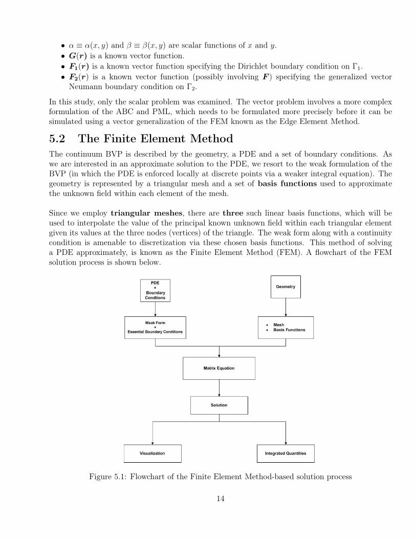
5.2 The Finite Element MethodThe continuum BVP is described by the geometry, a PDE and a set of boundary conditions. Aswe are interested in an approximate solution to the PDE, we resort to the weak formulation of theBVP (in which the PDE is enforced locally at discrete points via a weaker integral equation). Thegeometry is represented by a triangular mesh and a set of basis functions used to approximatethe unknown field within each element of the mesh.

Since we employ triangular meshes, there are three such linear basis functions, which will beused to interpolate the value of the principal known unknown field within each triangular elementgiven its values at the three nodes (vertices) of the triangle. The weak form along with a continuitycondition is amenable to discretization via these chosen basis functions. This method of solvinga PDE approximately, is known as the Finite Element Method (FEM). A flowchart of the FEMsolution process is shown below.

Figure 5.1: Flowchart of the Finite Element Method-based solution process

14

This discretization yields a set of linear equations, the solution to which gives the values of theprincipal unknown field at all the nodes of all triangular elements forming the mesh. Once thenodal values are known, the value of the unknown field at any point in the solution domain can bedetermined by interpolation using the basis functions. The FEM can thus be used to find the totalfield in the vicinity of a scatterer. Since the incident field in a scattering scenario is known apriori,the method can be used to determine the scattered field as well.

In summary, the FEM consists of the following four major steps:

• Discretization: breaking up the solution region into a finite number of elements (meshes).

• Derivation of Governing Equations: derivation of governing equations for a typical ele-ment.

• Assembly: assembling of all elements in the solution region.

• Solution: solving the system of equations obtained.

The mathematical details of the Finite Element Method and how it is to be set up are described inAppendix A.

5.3 MeshingThree approaches were used for meshing:

1. Concentric Ring Meshing: this approach was used for circular objects in 2D.2. DistMesh based Meshing: this approach was used to mesh arbitrary objects in 2D for which

a signed distance function could be easily obtained analytically.3. COMSOL based Meshing: for very complicated objects that cannot be described using signed

distance functions, the COMSOL Multiphysics interface with MATLAB was used as a com-putational front-end for meshing.

5.3.1 Concentric Ring Meshing for circular objectsIn order to solve for the total electric field in the near region of a PEC Cylinder when an incidentplane wave strikes it, a meshing algorithm was evolved for circular solution domains. The details ofthis meshing algorithm are described below, with reference to the particular geometry under study.

A PEC Cylinder of radius ρ = a is centered at the origin. The solution domain extends fromρ = a to ρ = ρABC , where ρABC is the radius of the circular boundary over which the AbsorbingBoundary Condition is to be enforced. The region from ρ = 0 to ρ = ρABC is divided into Nring

annular rings, with Nring given by

Nring =

⌈ρABC − a√

3h2

⌉(5.9)

where h is the discretization size. The differential step change in the radial direction is given by

∆ρ =ρABC − aNring

(5.10)

15

At a fixed ρ (where ρ = a : ∆r : ρABC), the angular separation between two successive nodes isgiven by

∆φ =2π

Npts

(5.11)

where Npts = d2πρ/he is the total number of nodes on the boundary of the segment at radius ρ. Asρ increases, the angular spacing between two successive nodes reduces, because the total number ofnodes on the boundary increases with its radius. By following this procedure, nodes are “marked”on the solution domain, and triangulation using the MATLAB function delaunay populates theannular regions by as many equilateral triangles of side length h as possible, with the remainingregion being filled up with skewed triangles.

Triangles located in the region interior to the PEC which are rendered by the triangulation sub-routine, must be removed as this region is excluded from the solution domain. The local nodenumbering generated by this subroutine is not always counterclockwise as required by the FEM for-mulation (c.f. Figure 7.1), so a reordering of the nodes is carried out to bring them to the canonicalorientation. A generalization to dielectric objects is described below.

The inputs to the meshing algorithm are

• ρcyl (or a): the radius of the PEC• ρABC : the radius of the circular boundary over which the ABC is to be imposed• h : the discretization size (a measure of the equilateral triangle side, in units of wavelength)

The outputs of the meshing algorithm are

• nNodes: Number of Nodes• nElements: Number of elements• N(e, i): Connectivity array (described in Appendix A).• x(i), y(i): x- and y-coordinates of the nodes.

A triangular mesh pattern for ρcyl = a = 0.5λ, ρABC = 1.5λ and h = 0.09 generated using the abovealgorithm is shown below.

Figure 5.2: Triangular Mesh Pattern for h = 0.09

16

Points to note:

1. In order to generalize concentric ring meshing to non-PEC (i.e. dielectric) objects, all we needto do is set a = 0 in equations (4.9 − 4.11), with the understanding that the region interiorto the dielectric cylinder is also to be meshed. Different values of h could be specified for thetwo regions, if desired.

2. For a mesh to be a valid input to the FEM code block, it is important that the local nodenumbering of each triangle be consistent with the counterclockwise numbering conventiondescribed in Appendix A, failing with the FEM matrices become singular, resulting in severelyerroneous solutions.

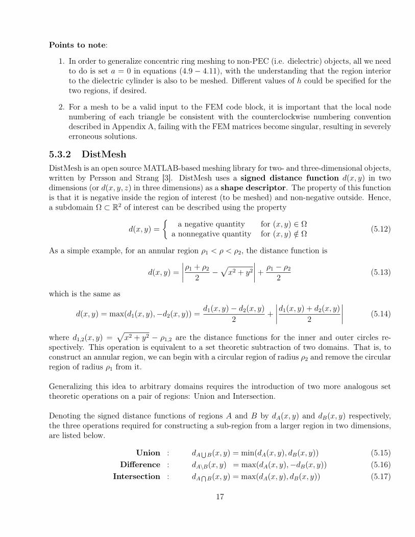
5.3.2 DistMeshDistMesh is an open source MATLAB-based meshing library for two- and three-dimensional objects,written by Persson and Strang [3]. DistMesh uses a signed distance function d(x, y) in twodimensions (or d(x, y, z) in three dimensions) as a shape descriptor. The property of this functionis that it is negative inside the region of interest (to be meshed) and non-negative outside. Hence,a subdomain Ω ⊂ R2 of interest can be described using the property

d(x, y) =

a negative quantity for (x, y) ∈ Ω

a nonnegative quantity for (x, y) /∈ Ω(5.12)

As a simple example, for an annular region ρ1 < ρ < ρ2, the distance function is

d(x, y) =

∣∣∣∣ρ1 + ρ2

2−√x2 + y2

∣∣∣∣+ρ1 − ρ2

2(5.13)

which is the same as

d(x, y) = max(d1(x, y),−d2(x, y)) =d1(x, y)− d2(x, y)

2+

∣∣∣∣d1(x, y) + d2(x, y)

2

∣∣∣∣ (5.14)

where d1,2(x, y) =√x2 + y2 − ρ1,2 are the distance functions for the inner and outer circles re-

spectively. This operation is equivalent to a set theoretic subtraction of two domains. That is, toconstruct an annular region, we can begin with a circular region of radius ρ2 and remove the circularregion of radius ρ1 from it.

Generalizing this idea to arbitrary domains requires the introduction of two more analogous settheoretic operations on a pair of regions: Union and Intersection.

Denoting the signed distance functions of regions A and B by dA(x, y) and dB(x, y) respectively,the three operations required for constructing a sub-region from a larger region in two dimensions,are listed below.

Union : dA⋃B(x, y) = min(dA(x, y), dB(x, y)) (5.15)

Difference : dA\B(x, y) = max(dA(x, y),−dB(x, y)) (5.16)Intersection : dA

⋂B(x, y) = max(dA(x, y), dB(x, y)) (5.17)

17

The operations mentioned above are described geometrically in the figure below.

Figure 5.3: Set Theoretic Operations on Regions using Signed Distance Functions

DistMesh uses an algorithm that combines a physical principle of force equilibrium in a truss struc-ture with a mathematical representation of the geometry using signed distance functions [15]. Theiterative technique is based on the physical analogy between a simplex mesh and a truss structure.

Meshpoints are nodes of the truss. Assuming an appropriate force-displacement function for thebars in the truss at each iteration, the algorithm solves for an equilibrium condition. The forcesmove the nodes and iteratively, the Delaunay triangulation algorithm adjusts the topology.

The basic algorithm employed by DistMesh is described below, step-by-step.

1. Create a uniform distribution of nodes within the bounding box of the geometry, correspondingto equilateral triangles.

2. Remove all nodes outside the desired geometry (using the signed distance function’s negativityas a criterion for interioricity).

3. Now, enter the main loop where the location of the nodes is iteratively improved until equi-librium is reached.

(a) Perform a Delaunay triangulation on the existing node set to determine the topology ofthe truss at this iteration.

(b) Now, evaluate the force function. If equilibrium is attained, break. otherwise, determinethe extent of movement of the nodes in this iteration and reiterate until equilibrium.

4. Determine the list of triangles which is a ne × 3 matrix (where ne is the total number oftriangular elements), and the node coordinates x and y, after removing duplicate entries.

5. Determine the the boundary edges, for imposing Dirichlet, Neumann and Mesh Truncationconditions.

18

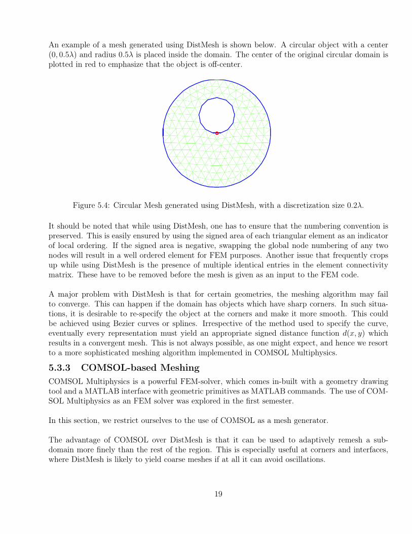
An example of a mesh generated using DistMesh is shown below. A circular object with a center(0, 0.5λ) and radius 0.5λ is placed inside the domain. The center of the original circular domain isplotted in red to emphasize that the object is off-center.

Figure 5.4: Circular Mesh generated using DistMesh, with a discretization size 0.2λ.

It should be noted that while using DistMesh, one has to ensure that the numbering convention ispreserved. This is easily ensured by using the signed area of each triangular element as an indicatorof local ordering. If the signed area is negative, swapping the global node numbering of any twonodes will result in a well ordered element for FEM purposes. Another issue that frequently cropsup while using DistMesh is the presence of multiple identical entries in the element connectivitymatrix. These have to be removed before the mesh is given as an input to the FEM code.

A major problem with DistMesh is that for certain geometries, the meshing algorithm may failto converge. This can happen if the domain has objects which have sharp corners. In such situa-tions, it is desirable to re-specify the object at the corners and make it more smooth. This couldbe achieved using Bezier curves or splines. Irrespective of the method used to specify the curve,eventually every representation must yield an appropriate signed distance function d(x, y) whichresults in a convergent mesh. This is not always possible, as one might expect, and hence we resortto a more sophisticated meshing algorithm implemented in COMSOL Multiphysics.

5.3.3 COMSOL-based MeshingCOMSOL Multiphysics is a powerful FEM-solver, which comes in-built with a geometry drawingtool and a MATLAB interface with geometric primitives as MATLAB commands. The use of COM-SOL Multiphysics as an FEM solver was explored in the first semester.

In this section, we restrict ourselves to the use of COMSOL as a mesh generator.

The advantage of COMSOL over DistMesh is that it can be used to adaptively remesh a sub-domain more finely than the rest of the region. This is especially useful at corners and interfaces,where DistMesh is likely to yield coarse meshes if at all it can avoid oscillations.

19

An example of a mesh generated for a complicated concave PEC object in 2D is shown below:

Figure 5.5: Mesh for a concave PEC object generated using COMSOL, with a discretization size0.2λ.

The exact internal details of COMSOL’s meshing algorithm are not known, and in this particularcase, COMSOL has been used more as a black box for meshing complicated objects, and transferringthe mesh to our own FEM codes, so that we have control over all the matrix elements. However, itis known that COMSOL uses Delaunay Triangulation for meshing.

5.4 Mesh TruncationIn order to apply the finite element method to open-region scattering or radiation problems, theinfinite solution domain must be truncated into a finite one. This is a fundamental requirementof any computational solution due to the restriction of finite memory on a computational engine.Geometric truncation implies the imposition of boundary conditions which force the solution toevolve within the reduced geometry. However, such forced terminations can introduce additionalartifacts into the solution due to reflection, scattering, etc. The problem then, is to determine sucha termination that does not introduce undesirable properties in the scattered fields of interest in thesolution domain, and at the same time, prevents them from differing considerably from the solutionin the physical unbounded space.

Now, assuming that all sources and objects are immersed in free space and located within a fi-nite distance from the origin of a coordinate system, the electric and magnetic fields are requiredto satisfy the Sommerfeld Radiation Condition [1],

limr→∞

r

[∇×

(EH

)+ jk0r ×

(EH

)]= 0 (5.18)

which in two dimensions becomes

limρ→∞

√ρ

[∂

∂ρ

(EzHz

)+ jk0

(EzHz

)]= 0 (5.19)

20

But this condition is no longer valid since the solution domain has been artificially truncated bysome boundary which is located at a finite distance from the scatterer. So, we need to enforcea suitable boundary condition on this artificial boundary such that a perfect absorbing surface issimulated. That is, the EM modes in the region see a “transparent” surface, and do not sufferreflection. This gives the impression that the solution domain is unbounded whereas it is in factfinite, and hence representible on a computer system with finite memory size.

The first order absorbing boundary condition in two dimensions is given by,

∂φsc

∂ρ+

(jk0 +

1

2ρ

)φsc = 0 (5.20)

whereas the second order absorbing boundary condition is given by,

∂φsc

∂n+

[jk0 +

κ

2− jκ2

8(jκ− k0)

]φsc − j

2(jκ− k0)

∂2φsc

∂s2= 0 (5.21)

where ∂/∂n denotes the derivative normal to the scattering surface (in 2D cylindrical coordinates,n = ρ) and ∂2/∂s2 denotes the second order tangential derivative (in 2D cylindrical coordinates,s = ρϕ). Also, κ = 1/ρ is the curvature of the 1-surface. This is the Bayliss-Gunzberger-TurkelABC [6]. In Appendix B, it is shown that the first order ABC can be directly included in theFEM formulation. With a suitable redefinition of the intrinsic boundary condition in the FEM, thesecond order ABC can also be similarly included, as described in Appendix C.

In two dimensions, the scattered field in the far field zone has the asymptotic form

φsc(ρ, ϕ) = A(φ)e−jkρ√ρ

(5.22)

The important feature of this asymptotic solution is that it falls of as 1/√ρ and not exponentially

with distance. The first order absorbing boundary condition (ABC) can be rewritten as

∂φsc

∂ρ=

(−jk − 1

2ρ

)φsc (5.23)

The convergent expansion for the solution of the Helmoltz equation satisfying the Sommerfeldradiation condition [1] is given by,

φsc(ρ, ϕ) = H(2)0 (kρ)

∞∑n=0

fn(ϕ)

ρn+H

(2)1 (kρ)

∞∑n=0

gn(ϕ)

ρn(5.24)

where H(2)0 and H(2)

1 denote the zeroth- and first-order Hankel functions of the second kind, respec-tively. Using the asymptotic form for the Hankel functions, we can write this as

φsc(ρ, ϕ) =e−jkρ√ρ

∞∑n=0

an(ϕ)

ρn(5.25)

21

From this we can obtain the second order ABC by neglecting terms of order O(ρ−9/2) in the followingexpression

∂φsc

∂ρ=

(−jk − 1

2ρ+

1

8jkρ2+

1

8k2ρ3

)φsc +

(1

2jkρ2+

1

2k2ρ3

)∂2φsc

∂ϕ2+O

(1

ρ9/2

)(5.26)

There are limitations to the ABC however. Strictly, such an ABC can only be enforced on acircular boundary. This is because of the ill-posed definition of a second order curvature termover nonsmooth boundaries.

Further, since an ABC aims to model a reflectionless surface, it cannot be very close to the scat-terer. In fact, the farther away from the scatterer the ABC is imposed, the more accurate theFEM solution will be. But doing so will increase the amount of data storage enormously. Althoughin principle it is possible to reduce the problem size by using a higher order ABC, the tradeoffbetween space complexity and time complexity will remain since higher order ABCs willrequire the computation of higher order field derivatives, both tangential as well as normal.

Also, it is known that the Absorbing Boundary Condition runs into difficulties with interfaces,because of the typical assumption of a homogeneous region around the scatterer. Finally, the ABCis perfectly absorbing only for a plane wave, which is not physically realizable.

Hence, we resort to another form of mesh truncation, known as a Perfectly Matched Layer (PML)[8, 10, 11, 12]. Strictly, a PML is not a boundary condition but rather an additional domain thatabsorbs incident radiation without producing reflections.

Figure 5.6: (a) the unbounded problem, and (b) the geometry augmented with a PML.

The figure on the left indicates the geometry of the original BVP. On the right, the solution domainhas been truncated all round by the use of a perfectly absorbing layer that is reflectionless. Thus,we are looking for a layer of (artificial) material to enclose our region of interest in such a way thatthe fields under study in that region do not “see” this layer. This is a difficult problem in itself, asa reflectionless layer enclosing the entire solution domain is difficult to develop in the absence ofinformation about the very fields it must fail to reflect. It should be noted that this layer is artificial.

22

A PML is developed using a three-step process, described by Johnson [8] and illustrated in thefigure below:

Figure 5.7: The three step-process for setting up a PML

1. In infinite space, we analytically continue the solutions and equations to a complex x contour.This changes oscillating waves into exponentially decaying waves outside the region of interestwithout reflections.

2. Still in infinite space, we perform a coordinate transformation to express the complex x as afunction of a real coordinate. In these new coordinates, we have real coordinates and complexmaterials.

3. We truncate the domain of this new real coordinate inside the complex-material region: sincethe solution is decaying there, as long as we truncate it after a long enough distance (wherethe exponential tails are small), the boundary condition used will not significantly impact thefinal solution. So, even hard-wall truncations are acceptable.

The hard-wall truncation at the outer surface of the layer can be effected using a simple Dirichletcondition for a PEC, for example, incurring minimal (of course, unavoidable) reflections there. It isknown [8] that the PML can be incorporated by the following differential operator transformations

∂

∂x→ 1

1 + iσx(x)ω

∂

∂x(5.27)

∂

∂y→ 1

1 + iσy(y)

ω

∂

∂y(5.28)

23

The artificial PML material is seen to have both an electrical as well as a magnetic conductivity dueto the existence of terms corresponding to currents of electric and magnetic charges. Despite thelimitations of the PML (multiple angle absorption, numerical reflections due to discretization, andthe existence of some inhomogeneous media where the PML fails to act as a reflectionless layer), itsfeatures and apparent simplicity in implementation over the standard homogeneous ABCs discussedabove are suggestive of its utility in the half-space subsurface scattering problem.

To summarize, imposing a PML for mesh truncation is equivalent to modifying the differentialoperator in the original BVP in a local region of the solution domain, so as to obtain an artificialmedium with finite electric and magnetic conductivity (and absorption). This medium convertsoscillating complex exponentials into decaying real exponentials due to the analytic continuationof space. To this extent, the PML is another way of enforcing an absorbing boundary condition,but without forcing the scattered field itself to satisfy a mixed boundary condition explicitly inthe solution domain. The PML formulation can be deduced from Maxwell’s equations by intro-ducing a complex-valued coordinate transformation with the additional requirement that the waveimpedance should remain unaffected.

In practice, the PML is typically used along with an absorbing boundary condition at its outer(unphysical) boundary. While a hard Dirichlet condition can also be used to terminate the fields,it acts as a reflector for any fields that may leak into the PML region. As this is undesirable, anabsorbing boundary condition of the first order can be used to avoid reflections of any remnantfields in the PML region. As demonstrated by the simulated results, a combination of PML andABC reduces the reflections induced by mesh truncation more effectively than purely a first orderABC.

24

Chapter 6

Methodology Adopted

In this project, we focused on solving the forward problem to compute the scattered electric fieldsand total field distributions for the following scenarios:

1. Perfect Electric Conducting (PEC) cylinder placed in air (vacuum).2. PEC concave object placed in air.3. PEC square object placed in air.4. Two PEC objects (concave + square) placed in air.5. Dielectric cylinder placed in air.6. PEC cylinder buried under the soil.7. Dielectric cylinder buried under the soil.

Mesh truncation schemes used were the first order ABC, the second order ABC and PerfectlyMatched Layers. Of these the first four problems were solved by writing our own computer pro-grams in MATLAB from scratch. For meshing circular and rectangular regions, we generated ourown codes. But for complicated geometries which can be described using signed distance functions,DistMesh can be used for meshing. For still more complicated geometries, such as concave objects,COMSOL’s meshing subroutines were used.

For the first four situations listed above, our own FEM codes were used with mesh truncationprovided by first order and second order ABCs. Both DistMesh and COMSOL were used solely asmesh generators in this class of problems. The mesh connectivity matrices generated by both theselibraries have to be suitably reordered for use in an FEM code. Therefore, interface code for bothDistMesh as well as COMSOL had to be written in MATLAB. The last three problems mentionedabove were formulated and simulated solely in COMSOL Multiphysics, an FEM-based modellingand visualization program.

Emphasis was placed on PEC objects to examine the performance of various mesh truncationschemes in the worst case scenario of a perfect reflecting surface in the path of an incidentfield. Specifically, PEC objects are near perfect reflectors of the incident field, and impose the sever-est possible boundary condition on the tangential electric field, that of forcing it to be identicallyzero on their surfaces. Naturally, if a mesh truncation scheme works well in case of PECs, it shouldwork well in case of dielectrics.

A contour plot of the electric field distribution for each of these cases is plotted in the next section.In this section, we formulate the scattering problem. Meshing has been described in section 4.3 ofthis report. The mathematical details of the Finite Element Method and the Absorbing BoundaryConditions, are described thoroughly in Appendices A through C. We now state the forward prob-lem formally for two inherently open region and closed region problems.

25

6.1 Statement of the Forward Problem (for Cylindrical PECObject in Air)

A perfect electric conductor, in the shape of a circular cylinder of radius a, is oriented in vacuum,with its axis along the z axis. A plane z-polarized electromagnetic wave of wavelength λ = 2π/k0,with an electric field amplitude E0 impinges on the cylinder normally,

Einc = azE0e−jk0x = azE0e

−jk0ρ cosφ (6.1)

and is scattered. It is required to find the total electric field (incident + scattered) as a function ofthe angle φ at a distance ρ = λ from the center of the cylinder. It is given that a = λ/2 and E0 = 1V/m.

6.1.1 The Partial Differential Equation for the Total Electric FieldThe incident E field is polarized along the z-direction, so the scattered E field from the infinitelylong cylinder is also polarized along the z-direction. Therefore, the total electric field E will haveonly a z-directed component: E = Eaz, and there will be no z-variations in the field:

∂Ez∂z

= 0 =⇒ E = Ez ≡ Ez(x, y) (6.2)

Consider the following two time-Harmonic Maxwell’s equations,

∇× E = −jωµ0µrH (6.3)∇×H = J + jωε0εrE (6.4)

Solving for H from (6.3) and substituting into (6.4), we get

− 1

jωµ0

∇×(

1

µr∇× E

)= J + jωε0εrE (6.5)

Due to (6.2) we also have

∇× E = ax∂Ez∂y− ay

∂Ez∂x

(6.6)

The curl term on the left hand side of (6.5) can be written as

∇×(

1

µr∇× E

)=

∣∣∣∣∣∣ax ay az∂∂x

∂∂y

∂∂z

1µr

∂Ez

∂y− 1µr

∂Ez

∂x0

∣∣∣∣∣∣ (6.7)

= az

[− ∂

∂x

(1

µr

∂Ez∂x

)− ∂

∂y

(1

µr

∂Ez∂y

)](6.8)

where, the condition ∂µr/∂z = 0 has been used to arrive at the second equality. Substituting (6.8)into (6.4) and simplifying, we get the Helmoltz equation

∂

∂x

(1

µr

∂Ez∂x

)+

∂

∂y

(1

µr

∂Ez∂y

)+ k2

0εrEz = jωµ0Jz (6.9)

26

where k20 = ω2µ0ε0. The source free version of this equation (for Jz = 0) has the same form as the

canonical scalar wave equation in the Galerkin formulation [1],

− ∂

∂x

(αx∂Φ

∂x

)− ∂

∂y

(αy∂Φ

∂y

)+ βΦ = f (6.10)

where,

αx = αy = − 1

µr(6.11)

Φ = Ez (6.12)β = k2

0εr (6.13)f = 0 (6.14)

6.2 Statement of the Forward Problem (for Buried Mines)Landmines are modelled as small abnormalities embedded in an otherwise uniform media with anair-ground interface. These abnormalities are characterized by the electrical permittivity ε and theconductivity σ, whose values differ from those of the host media.

The incident field is modeled here as a plane polarized wave with the electric field given by

Einc(r) = E0eiω√µ0ε0·y · e−iωt (6.15)

propagating in the negative y-direction in the half space y > 0. Here ω is the angular frequencyof the stimulus signal (ω = 2πf , where f ≈ 1GHz). It is assumed that y > 0 is air and y < 0is ground, where the mine-like targets are located.

The PDE for the forward problem in two dimensions, is

∇2Ez + k2(x, ω)Ez = 0 (6.16)

wherek2 =

ω2µrεrε0 for y > 0,ω2µrεrε0(1 + j tan δ) for y < 0

(6.17)

andtan δ =

σ(x, ω)

ωε(x)(6.18)

The free space wavenumber is k0 = ω√µ0ε0, and the free space wavelength is λ = 2π

Re(k)= 2π

k0.

27

6.2.1 Parameter ValuesThe simulations were carried out for two kinds of dielectric materials: dry and wet soil. All theparameters listed below are taken from Gryazin et al [13] and Huici et al [14]. These parametershave been listed for a frequency of 1GHz, which is the frequency at which all the buried minesimulations have been carried out.

Medium εr σ (S/m) tan δ k2 (m−2) k (m−1) λ (cm)Air 1 0 0 439.2 20.9 30Dry Soil 2.9 0.004 0.025 1273 + j31 35.7 + j0.43 17Wet Soil (5% moisture) 4 0.049 0.22 1756 + j395 42 + j4.7 15TNT 2.86 2.864× 10−4 0.0018 1256 + j2.26 35.4 + j0.03 17.7

Table 1: Approximate values of εr, tan δ, k2, k and λ for different soil moistures and TNT at f = 1GHz.

Description of Quantities

• εr: Relative permittivity of the medium.• σ (S/m): Conductivity.• tan δ: Loss tangent (given by eqn. 6.18).• k (m−1): Propagation constant.• k0 (m−1): Propagation constant in free space.• λ (m): Free space wavelength. λ = 2π

Re(k).

The values for TNT (Trinitrotoluene) are listed as being representative of a land mine buried inthe ground, as TNT is an explosive substance. Two kinds of soil, differing in moisture content (andtherefore in dielectric properties), have been considered here to examine the contrast with with theburied mine can be imaged in both scenarios. The results of the simulations carried out in ComsolMultiphysics, are mentioned in the “Results” section of this report. The contrast of the buried mineis enhanced when it is buried under wet soil, as indicated by the scattered field distribution.

28

Chapter 7

Results

7.1 Circular PEC Object centered at the originThe first object to be considered has a radius a = λ/2 where λ is the free space propagation wave-length. The first order ABC is imposed at 3λ/2, a wavelength away from the object. The incidentfield has the form E0e

−jk0x for E0 = 1V/m, k0 = 2π/λ. All distances are normalized with respectto λ. So without loss of generality, λ = 1.

For this particular problem, the concentric ring based meshing algorithm described above wasused. A plot of the total electric field as a function of the polar angle at a radius ρ = λ, is shownbelow on the left, for various values of the mesh discretization parameter h (expressed in units ofλ).

Figure 7.1: First and Second Order solutions for PEC Cylinder Scattering for discretization sizesλ/2, λ/5, λ/10, and λ/25, all evaluated at ρ = λ.

The same experiment was then repeated but with a second order ABC imposed on a mesh truncationboundary, rather than the first order condition. The corresponding plot of the total electric field isshown in the figure on the right above. This problem has an analytical solution [7], given by

Ez(ρ, θ) = E0

∞∑n=−∞

j−n

[Jn(k0ρ)− Jn(k0a)

H(2)n (k0a)

H(2)n (k0ρ)

]ejnθ (7.1)

29

where Ez denotes the z-component of the total electric field, a is the radius of the PEC cylinder,and ρ and θ are the cylindrical polar coordinates. Here, Jn denotes the Bessel Function of the FirstKind of order n and H(2)

n denotes the Hankel Function of the Second Kind of order n.

The absolute values of the exact, first order and second order solutions are plotted in the figurebelow, for a discretization size of λ/25, on the boundary ρ = λ.

Figure 7.2: Analytical and FEM Solutions for the PEC Cylindrical Scatterer, at discretization λ/25,evaluated at ρ = λ

From the plots, we can infer that

1. Both 1st and 2nd order ABC solutions become smoother as the discretization size is lowered.2. For a discretization size of λ/25, the 2nd order ABC-based solution almost coincides with the

analytical solution, whereas the 1st order ABC-based solution deviates from the analyticalsolution more significantly at very small angles (≈ 0o), moderately large angles (100o and260o) and again at around 360o. The solution is naturally symmetric about the x-axis.

Clearly, the 2nd-order ABC-based solution more closely approximates the total electric field thanthe 1st-order ABC based solution.

30

7.2 Location of 2nd order ABC vs. that of 1st order ABCThe total electric field was computed using both the 1st and 2nd order ABC. The 1st order ABCwas imposed at a distance ρ = 2λ whereas the 2nd order ABC was imposed at ρ = 1.5λ, with thediscretization for both situations taken to be 0.04λ.

The total electric field at ρ = λ is plotted below, as a function of the polar angle. It is evi-dent that both the numerical solutions are almost comparable, with the 2nd order solution moreclosely approximating the exact (analytical) solution. This demonstrates that the 2nd orderABC gives a more accurate solution even when imposed at a boundary closer to thescatterer.

Figure 7.3: Electric Field at ρ = λ

The table below illustrates the advantage gained by using the 2nd order ABC over the 1st order ABC.As is evident from the numerical values, the 2nd order ABC yields a solution comparable to (if notslightly better than) the 1st order ABC, despite using about half the number of nodes and elements.

Parameter First Order ABC at 2λ Second Order ABC at 1.5λNo. of nodes 1843 984No. of elements 3511 1828No. of Dirichlet Nodes 35 35No. of ABC Nodes 140 105

Table 2: Comparison of matrix sizes for 1st and 2nd order ABC.

31

7.3 Circular PEC Object placed off centerThe domain consists of a circular object of radius 0.5λ, centered at (0, 0.5λ). The mesh, polar andcontour plots of the field are shown below. The contour plot confirms that the 2nd order solutionis smoother, and better preserves the symmetry of the object. The field very close to the PEC isexpected to be very nearly zero, which is more evident when the 2nd order ABC is used for meshtruncation.

Figure 7.4: Electric Fields near an off-center PEC Cylinder

Figure 7.5: Contour Plots of the Electric Field, using the 1st order ABC (left) and 2nd order ABC(right)

32

7.4 Concave PEC ObjectThe object was modelled using two elliptical arcs centered at (0.2λ, 0), with semi-axes of lengtha = 0.2λ, b = 0.5λ. The total electric field was computed using the 1st and 2nd order ABCs, atρ = λ is plotted on the right, above.

Figure 7.6: Electric Fields near a Concave PEC Object

Contour plots of the total electric field in the vicinity of the concave PEC scatterer are plottedbelow. Although mostly comparable, the electric field in the near region of the PEC in the forwardscattering direction, is seen to spread backwards less in case of the 2nd order solution. This isconsistent with the fact that a PEC strongly suppresses forward scattering.

Figure 7.7: Electric Field Contours for Scattering from a Concave PEC Object, using the 1st orderABC (left) and the 2nd order ABC (right).

33

7.5 Square PEC Object placed off centerA PEC object with a square cross-section of side 0.5λ was placed with its bottom left corner at theorigin. The resulting mesh pattern is shown below.

Figure 7.8: Mesh for a Square PEC Object.

Contour plots of the total electric field in the vicinity of the square object are plotted below. The2nd order solution is seen to be more regular and smoother near the PEC, and also preserves thesymmetry of the object.

Figure 7.9: Electric Field Contours for Scattering from a Square PEC Object, using the 1st orderABC (left) and the 2nd order ABC (right).

34

7.6 Two PEC ObjectsThe framework developed also allows us to examine the field patterns due to the presence of multipleobjects - a more practical scenario. As an example, we consider two objects, as shown in the mesheddomain below. The domain consists of a concave object and a square of edge length 0.2λ with thetop left corner at the origin.

Figure 7.10: Mesh for double PEC object scattering

Contour plots of the total electric field are shown below. The 2nd order ABC-based solution is muchbetter than the one based on the 1st order ABC, because it is much more regular and smoother,and evaluates a very small electric field in the immediate vicinity of the scatterer, an observationconsistent with the properties of a PEC.

Figure 7.11: Contour Plots for Scattering from two PEC objects, using the 1st order ABC (left)and 2nd order ABC (right)

35

7.7 Comparison between 1st order ABC and PML PEC Cylin-der in Air

Comsol Multiphysics was used for simulation, and the 1st order ABC and PML were implementedand compared at four frequencies: 0.5GHz, 1GHz, 1.5GHz and 3GHz. In this case, the excitationplane wave is incident from the top. The results are shown below.

Figure 7.12: Scattered Fields from PEC Cylinder in Air: ABC vs PML

The solution is seen to be smoother with the PML in place, than just with the First Order ABC,due to better absorbing characteristics of the PML. Comsol also plots the scattered field within thePEC, which is not plotted conventionally. This should be ignored.

36

7.8 Comparison between ABC and PML for Dielectric Cylin-der in Air

In this case, a dielectric cylinder with relative permittivity εr = 2.86 and conductivity σ = 2.864×10−4S/m, is placed in air. As before, the excitation plane wave propagates along the negativey-direction.

Figure 7.13: Scattering from Dielectric Cylinder in Air: ABC vs PML

As with the PEC, the solution is seen to be smoother with the PML in place, than just with the FirstOrder ABC, due to better absorbing characteristics of the PML. Comsol also plots the scatteredfield within the PEC, which is not plotted conventionally. This should be ignored.

37

7.9 The Subsurface Problem (Half Space Scattering)In this case, a simplified version of the situation portrayed in Figure 1.1, was modeled and solved inComsol Multiphysics, for two possible objects buried under the soil (a PEC cylinder and a dielectriccylinder), and two kinds of soil (dry and wet soil). The results are given below. In the subsurfaceproblem, we use the combined ABC-PML method throughout. The frequency of the incident waveis 1.0GHz in each case.

7.10 PEC Cylinder buried under SoilA PEC Cylinder of radius r = 5 cm is placed at a depth of 10 cm below the surface of the soil. Thesimulation was carried out for two kinds of soil, dry and wet. The mesh truncation scheme involvesusing PML on the inner rectangular boundaries, and a first order ABC on the outer rectangularboundaries.

Figure 7.14: Scattering from PEC Cylinder buried under Soil (z-component of total field for drysoil (left) and wet soil (right).)

38

7.11 Dielectric Cylinder buried under SoilA Dielectric Cylinder of relative permittivity εr = 2.86, conductivity σ = 2.864× 10−4S/m havinga radius r = 5 cm is placed at a depth of 10 cm below the surface of the soil. The simulation wascarried out for two kinds of soil, dry and wet. The mesh truncation scheme involves using PML onthe inner rectangular boundaries, and a first order ABC on the outer rectangular boundaries.

Figure 7.15: Scattering from Dielectric Cylinder buried under Soil (z-component of total field fordry soil (left) and wet soil (right).

It is observed that the contrast of the mine increases as the soil becomes more wet, whether the mineis a PEC or a dielectric (TNT). This is consistent witht he increased conductivity and dielectricconstant of moist soil, tends to concentrate the scattered field.

Note: The contour plots in sections 7.7-7.11 are reproduced after magnification inAppendix D, for greater ease of viewing and clarity.

39

7.12 Scattering from a PEC Cylinder in Air using the FirstOrder ABC (Effect of varying Discretization)

For a PEC cylinder of radius λ/2, and an ABC boundary of radius 3λ/2, the analytical and FEMsolutions are compared at ρ = λ, for different discretizations, to illustrate the effect of meshing.The mesh pattern, a contour plot of the total electric field in the region, and a graph of the FEMand exact solution have been plotted for three discretization sizes, and the results are shown below.

Fig. a: Discretization Size= 0.2

Fig. b: Discretization Size= 0.09

Fig. c: Discretization Size= 0.04

It is seen that for ρcyl = a = 0.5λ, ρABC = 1.5λ, the FEM solution is very nearly equal to the exactsolution for the discretization size 0.04. The entire source code for solving this problem is given inthe appendices of this report.

40

Chapter 8

Conclusions

A framework for solving the Laplace, Poisson and Helmoltz equations in two dimensions has beenconstructed from scratch in MATLAB, comprising of meshing, preprocessing and FEM routines,with a feature to impose Mixed Boundary Conditions, in particular, the 1st and 2nd order ABCs.As a part of this project, a system for meshing of arbitrary shapes in two dimensions has been putin place by combining our own codes with DistMesh and COMSOL for meshing.

Completely general FEM codes have been written to compute the total and scattered field dis-tributions in the near region of one or more scatterers in two dimensional domains. Results fromseveral electromagnetic scattering situations have been mentioned and discussed in this report,comparing the 1st and 2nd order ABCs. Exact analytical expressions for 1st and 2nd order ABCshave been derived in Appendices B and C. These are directly used in an FEM code, and allow theprogrammer to have complete flexibility while solving a problem computationally.

Using COMSOL Multiphysics as an FEM modelling package, contour plots of the scattered fieldsfor PEC and dielectric cylinders in air and soil were extracted by simulation, results of which havebeen stated here.

Further work needs to be done to include codes for a generalized Perfectly Matched Layers inthis framework, and validate results obtained using COMSOL-based PMLs, so as to have com-plete acesss to and control over all the element matrices and vectors in the formulation of theFinite Element Method (Appendix A). The following inferences can be made from analytical andcomputational studies:

1. The 2nd order ABC is better than the 1st order ABC as for mesh truncation, as it introducesfewer artifacts in the computational solution, by capturing the curvature of the field.

2. The 2nd order ABC can be imposed at a smaller distance from the scatterer, thanthe 1st order ABC, without compromising fidelity of the solution.

3. The Second Order ABC used by us can be imposed only on circular boundaries.We observed that the second order curvature term contributes to large oscillations in the field,when evaluated over nonsmooth countours, leading to severe errors in the results.

4. For circular objects, the concentric ring meshing algorithm, described in section 4.3.1 yieldsbetter solutions than those provided by DistMesh and COMSOL. This is because of thesymmetry of the concentric ring mesh coinciding with the symmetry of the object geometry.

5. The PML-based mesh truncation scheme is better than the one using only a First Order ABC.

6. The contrast of scattered field distribution in the near region of the scatterer is enhanced asthe moisture content in the soil increases.

41

References

1. J. Jin, The Finite Element Method in Electromagnetics. New York: John Wiley & Sons, 1993.2. A.C. Polycarpou, Introduction to the Finite Element Method in Electromagnetics. San Rafael:

Morgan & Claypool Publishers, 2006.3. P. Persson and G. Strang, “DistMesh A Simple Mesh Generator in MATLAB,” SIAM Review,

vol. 46, no. 2, pp. 329-345, June 2004.4. J.L. Volakis, A. Chatterjee, and L.C. Kempel, Finite Element Method for Electromagnetics:

Antennas, Microwave Circuits, and Scattering Applications. Hyderabad: Universities Press(India) Pvt. Ltd., 2001.

5. S. Kesavan, Topics in Functional Analysis and Applications. New Delhi: New-Age Int’l., 2008.6. A. Bayliss, M. Gunzburger and E. Turkel, “Boundary conditions for the numerical solution of

elliptic equations in exterior regions,” SIAM J. Appl. Math., vol. 42, no. 2, April 1982.7. C.A. Balanis, Advanced Engineering Electromagnetics. New York: John Wiley & Sons, 1989.8. Steven G. Johnson, “Notes on Perfectly Matching Layers (PMLs) [MIT Course 18.369/18.336],”

August 2007. [Online]. Available: http://www-math.mit.edu/~stevenj/18.369/pml.pdf.9. J.L. Volakis and A. Chatterjee, “A selective review of the finite element-ABC and the finite

element-boundary integral methods for electromagnetic scattering,” Ann. Telecommun., vol.50, no. 5-6, pg. 499-509, May 1995.

10. J.P. Bérenger, “A Perfectly Matched Layer for the absorption of electromagnetic waves,” J.Comput. Phys., vol. 114, no. 2, pp. 185-200, October 1994.

11. C.M. Rappaport and S. Winton, “Using the PML ABC for air-soil wave interaction modelingin the time and frequency domains,” Int’l J. of Susburf. Sensing Tech. and Appl., vol. 1, no.3, pp. 289-304, July 2000.

12. J. Jin and W.C. Chew, “Combining PML and ABC for the Finite-Element analysis of scat-tering problems,” Microwave Opt. Tech. Lett., vol. 12, no. 4, pp. 192-197, July 1996.

13. Y.A. Gryazin, M.A. Klibanov, and T.R. Lucas, “Two numerical methods for an inverse problemfor the 2-D Helmoltz equation,” J. Comput. Phys., vol. 184, no. 1, pp. 122-148, Jan. 2003.

14. M.A. Gonzalez-Huici, U. Uschkerat, and A. Hoerdt, “Numerical simulation of electromagnetic-wave propagation for land mine detection using GPR,” Geoscience and Remote Sensing Sym-posium, July 23-28, 2007, Barcelona, Spain. IGARSS 2007. IEEE International.

15. Allan P. Engsig-Karup, “An introduction to Discontinuous-Galerkin FEM for partial dif-ferential equations,” August 2009. [Online]. Available: http://www2.imm.dtu.dk/~apek/DGFEMCourse2009/Material.php.

42

Appendix A: Finite Element MethodFormulation

We now examine the steps in a 2D FEM solution in some detail. We will assume for now thatthe meshing elements are triangular, with three nodes, which are the three vertices. The resultingmeshing scheme is known as Triangular Meshing. In the scalar situation, the objective is to solvethe boundary value problem,

− ∂

∂x

(αx∂φ

∂x

)− ∂

∂y

(αy∂φ

∂y

)+ βφ = f (x, y) ∈ Ω (8.1)

where φ is the unknown function, αx, αy, and β are known parameters associated with the physicalproperties of the domain Ω, and f is the source or excitation function. The boundary conditions tobe considered are given by

φ = p on Γ1 (8.2)

and (αx∂φ

∂xx+ αy

∂φ

∂yy

)· n+ γφ = q on Γ2 (8.3)

where Γ = Γ1+Γ2 denotes the contour or boundary enclosing Ω, n is its outward normal unit vector,and γ, p, and q are known parameters associated with the physical properties of the boundary. Thisis the Mixed Boundary Condition, and is a generalization of the Dirichlet and Neumann boundarycondition.

With a suitable meshing in place that breaks up the solution domain into N triangular meshes, weseek an approximation of φ = φe within each element e (e = 1, 2, . . . , N):

φ(x, y) ≈N∑e=1

φe(x, y) (8.4)

A common approximation for φe within element e is the first order polynomial expansion,

φe(x, y) = ae + bex+ cey (8.5)

where ae, be and ce are constants to be determined. An additional property of φe is that it vanishesoutside element e.

43

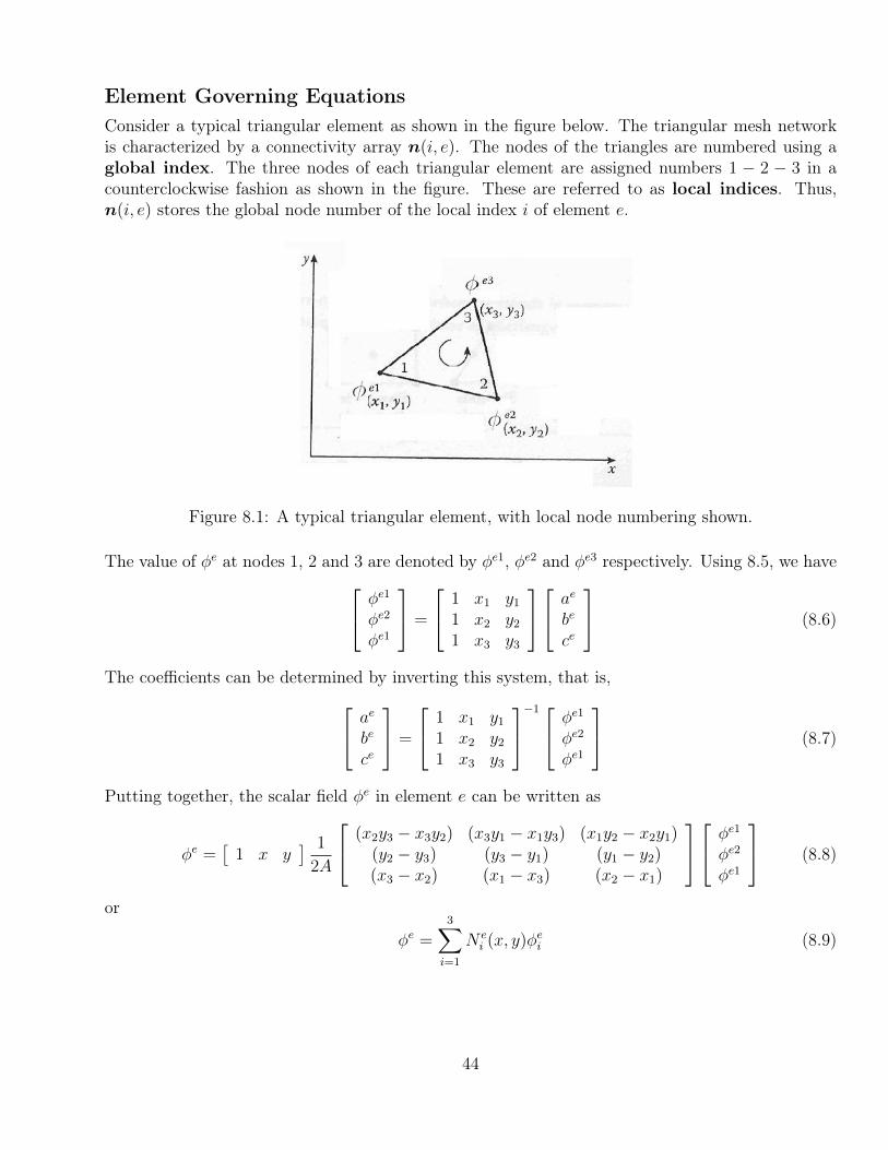
Element Governing EquationsConsider a typical triangular element as shown in the figure below. The triangular mesh networkis characterized by a connectivity array n(i, e). The nodes of the triangles are numbered using aglobal index. The three nodes of each triangular element are assigned numbers 1 − 2 − 3 in acounterclockwise fashion as shown in the figure. These are referred to as local indices. Thus,n(i, e) stores the global node number of the local index i of element e.

Figure 8.1: A typical triangular element, with local node numbering shown.

The value of φe at nodes 1, 2 and 3 are denoted by φe1, φe2 and φe3 respectively. Using 8.5, we have φe1

φe2

φe1

=

1 x1 y1

1 x2 y2

1 x3 y3

ae

be

ce

(8.6)

The coefficients can be determined by inverting this system, that is, ae

be

ce

=

1 x1 y1

1 x2 y2

1 x3 y3

−1 φe1

φe2

φe1

(8.7)

Putting together, the scalar field φe in element e can be written as

φe =[

1 x y] 1

2A

(x2y3 − x3y2) (x3y1 − x1y3) (x1y2 − x2y1)(y2 − y3) (y3 − y1) (y1 − y2)(x3 − x2) (x1 − x3) (x2 − x1)

φe1

φe2

φe1

(8.8)

or

φe =3∑i=1

N ei (x, y)φei (8.9)

44

where

N e1 (x, y) =

1

2A[(x2y3 − x3y2) + (y2 − y3)x+ (x3 − x2)y] (8.10)

N e2 (x, y) =

1

2A[(x3y1 − x1y3) + (y3 − y1)x+ (x1 − x3)y] (8.11)

N e3 (x, y) =

1

2A[(x1y2 − x2y1) + (y1 − y2)x+ (x2 − x1)y] (8.12)

and A is the area of the element e, given by

A =1

2

∣∣∣∣∣∣1 x1 y1

1 x2 y2

1 x3 y3

∣∣∣∣∣∣ =1

2[(x2 − x1)(y3 − y1)− (x3 − x1)(y2 − y3)] (8.13)

The value of A is positive if the nodes are numbered counterclockwise (starting from any node)as shown in the figure above. The N e

i ’s are known as element shape functions and satisfy thefollowing properties:

N ei (xej , y

ej ) = δij =

1, i = j0, i 6= j

(8.14)

3∑i=1

N ei (x, y) = 1 (8.15)

Weak FormThe weak form of the differential equation

− ∂

∂x

(αx∂φ

∂x

)− ∂

∂y

(αy∂φ

∂x

)+ βφ = f (8.16)

is

−∫ ∫

Ωe

[αx∂w

∂x

∂φ

∂x+ αy

∂w

∂y

∂φ

∂y

]dx dy +

∫ ∫Ωe

βwφ dx dy −∮

Γe

w

(αx∂φ

∂xnx + αy

∂φ

∂yny

)dl

=

∫ ∫Ωe

w f dx dy(8.17)

where nx and ny are the direction cosines of the normal to the surface. In the Galerkin approach,the weight functions w(x, y) are taken to be equal to the triangular interpolation functions used inthe FEM. 1

1The triangular shape functions are:

N1(ξ, η) = 1− ξ − ηN2(ξ, η) = ξ

N3(ξ, η) = η

The primary unknown quantity φ is interpolated within an element e as

φe(x, y) =

3∑j=1

φejNj(x, y)

Here φej denotes the value of the unknown quantity at local node j of element e.

45

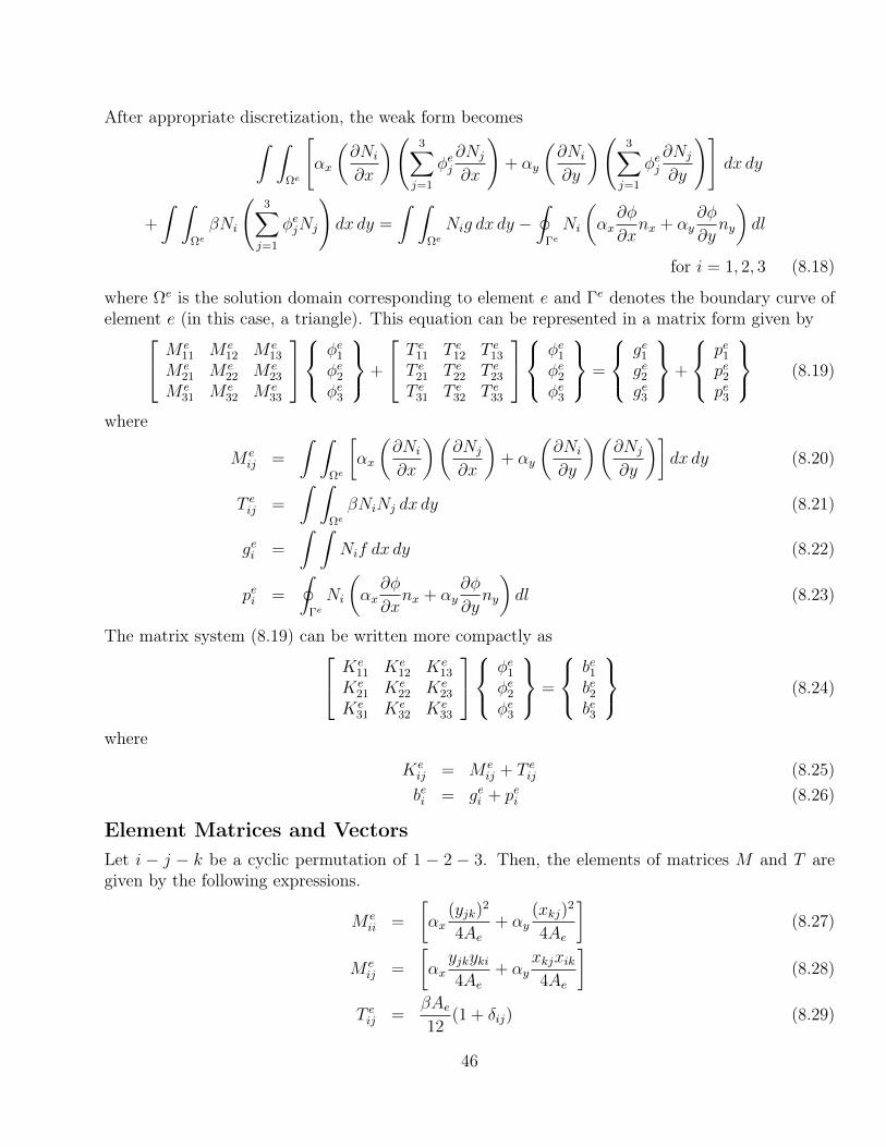
After appropriate discretization, the weak form becomes∫ ∫Ωe

[αx

(∂Ni

∂x

)( 3∑j=1

φej∂Nj

∂x

)+ αy

(∂Ni

∂y

)( 3∑j=1

φej∂Nj

∂y

)]dx dy

+

∫ ∫Ωe

βNi

(3∑j=1

φejNj

)dx dy =

∫ ∫Ωe

Nig dx dy −∮

Γe

Ni

(αx∂φ

∂xnx + αy

∂φ

∂yny

)dl

for i = 1, 2, 3 (8.18)

where Ωe is the solution domain corresponding to element e and Γe denotes the boundary curve ofelement e (in this case, a triangle). This equation can be represented in a matrix form given by M e

11 M e12 M e

13

M e21 M e

22 M e23

M e31 M e

32 M e33

φe1φe2φe3

+

T e11 T e12 T e13

T e21 T e22 T e23

T e31 T e32 T e33

φe1φe2φe3

=

ge1ge2ge3

+

pe1pe2pe3

(8.19)

where

M eij =

∫ ∫Ωe

[αx

(∂Ni

∂x

)(∂Nj

∂x

)+ αy

(∂Ni

∂y

)(∂Nj

∂y

)]dx dy (8.20)

T eij =

∫ ∫Ωe

βNiNj dx dy (8.21)

gei =

∫ ∫Nif dx dy (8.22)

pei =

∮Γe

Ni

(αx∂φ

∂xnx + αy

∂φ

∂yny

)dl (8.23)

The matrix system (8.19) can be written more compactly as Ke11 Ke

12 Ke13

Ke21 Ke

22 Ke23

Ke31 Ke

32 Ke33

φe1φe2φe3

=

be1be2be3

(8.24)

where

Keij = M e

ij + T eij (8.25)bei = gei + pei (8.26)

Element Matrices and VectorsLet i − j − k be a cyclic permutation of 1 − 2 − 3. Then, the elements of matrices M and T aregiven by the following expressions.

M eii =

[αx

(yjk)2

4Ae+ αy

(xkj)2

4Ae

](8.27)

M eij =

[αxyjkyki4Ae

+ αyxkjxik4Ae

](8.28)

T eij =βAe12

(1 + δij) (8.29)

46

Here Ae denotes the area of the triangular element e, and xij = xei −xej , yij = yei − yej . The elementsof vector ge are given by

ge1 =fAe

3(8.30)

ge2 =fAe

3(8.31)

ge3 =fAe

3(8.32)

if f does not appreciably vary over the element. A more general set of matrix equations for ageometry with Ne elements and Ms Dirichlet/Neumann segments is given by

Ne∑e=1

([Ke]φe − be) +Ms∑e=1

([Ks]φs − bs) = 0 (8.33)

where the matrices have been suitably augmented, and the individual elements are given by

Keij =

1

4Ae(αexb

ei bej + αeyc

ei cej) +

Ae

12βe(1 + δij) for i, j = 1, 2, 3 (8.34)

bei =

∫∫Ωe

f(x, y)N ei (x, y)dx dy for i = 1, 2, 3 (8.35)

Ksij =

∫ 1

0

γN siN

sj lsdξ for i, j = 1, 2 (8.36)

bsi =

∫ 1

0

γqN si lsdξ for i = 1, 2 (8.37)

This alternate system of equations is more useful if more general boundary conditionshave to be imposed. The values of the other matrix and vector elements are dependent on whethera first order ABC (Appendix B) is used or a second order ABC (Appendix C). Assuming that thematrix elements have been defined properly in accordance with the chosen absorbing boundarycondition, the remaining procedure is as follows.

Integration over an arbitrary triangular patchThe integral expression

bei =

∫∫Ωe

f(x, y)N ei (x, y)dx dy for i = 1, 2, 3 (8.38)

is zero in the total field formulation because f = 0 there, but if one works in the scattered fieldformulation, this term arises frequently. Also, if α or β vary inside an element, we have to use theintegral expression for Ke

ij itself, which involves a similar double integral. Since this integral is overan arbitrary triangular patch, the x and y integrals are coupled. We now give a nonlinear transfor-mation from an arbitrary triangular patch to a square which allows this integral to be carried outvery simply using numerical integration, for every element.

47

Consider the integral∫

Ωe g(x, y)dx dy. In order to simplify the numerical integration and not haveto consider various cases for the slopes of the edges of the triangular element, and its orientationwith respect to the axes, we define the following nonlinear transformation

x(u, v) = (1− u)xe1 + u [(1− v)xe2 + vxe3] (8.39)y(u, v) = (1− u)ye1 + u [(1− v)ye2 + vye3] (8.40)

This transformation maps the arbitrarily shaped and oriented triangular region Ωe in (x, y) spaceto a square in (u, v) space, that is (u, v) : 0 ≤ u ≤ 1, 0 ≤ v ≤ 1. The Jacobian matrix of thetransformation is given by

J =

(−xe1 + (1− v)xe2 + vxe3 −uxe2 + uxe3−ye1 + (1− v)ye2 + vye3 −uye2 + uye3

)(8.41)

Hence, the integral becomes∫∫Ωe

g(x, y)dxdy =

∫ 1

u=0

∫ 1

v=0

g(x(u, v), y(u, v))|J |dudv (8.42)

where

|J |(u, v) = (−xe1 + (1− v)xe2 + vxe3)(−uye2 + uye3)− (−ye1 + (1− v)ye2 + vye3)(−uxe2 + uxe3) (8.43)

Dirichlet Boundary ConditionsLet the prescribed values of φ be stored in a vector C(i) and let there by N ′ nodes on Γ1, whoseglobal node numbers are stored in a vector DBC(i). Then, the Dirichlet boundary condition isenforced by setting

bDBC(i) = C(i), KDBC(i),DBC(i) = 1, KDBC(i),j = 0 for j 6= DBC(i) (8.44)

bj ← bj −Kj,DBC(i)C(i), Kj,DBC(i) = 0 for j 6= DBC(i) (8.45)

for each i = 1, 2, . . . , N ′. In this problem, C(i) = 0 ∀ i = 1, 2, . . . , N ′.

Assembly of Ke, Ks into KThe first step is the assembly of Ke into K (for e = 1, 2, . . . nElements), the pseudocode for whichis given below.

Assemble Ke into K

1 for e← 1 to nElements2 do3 for i← 1 to 34 do5 for j ← 1 to 36 do K(N(e, i), N(e, j))← K(N(e, i), N(e, j)) +Ke(i, j)7 end for8 end for9 end for

48

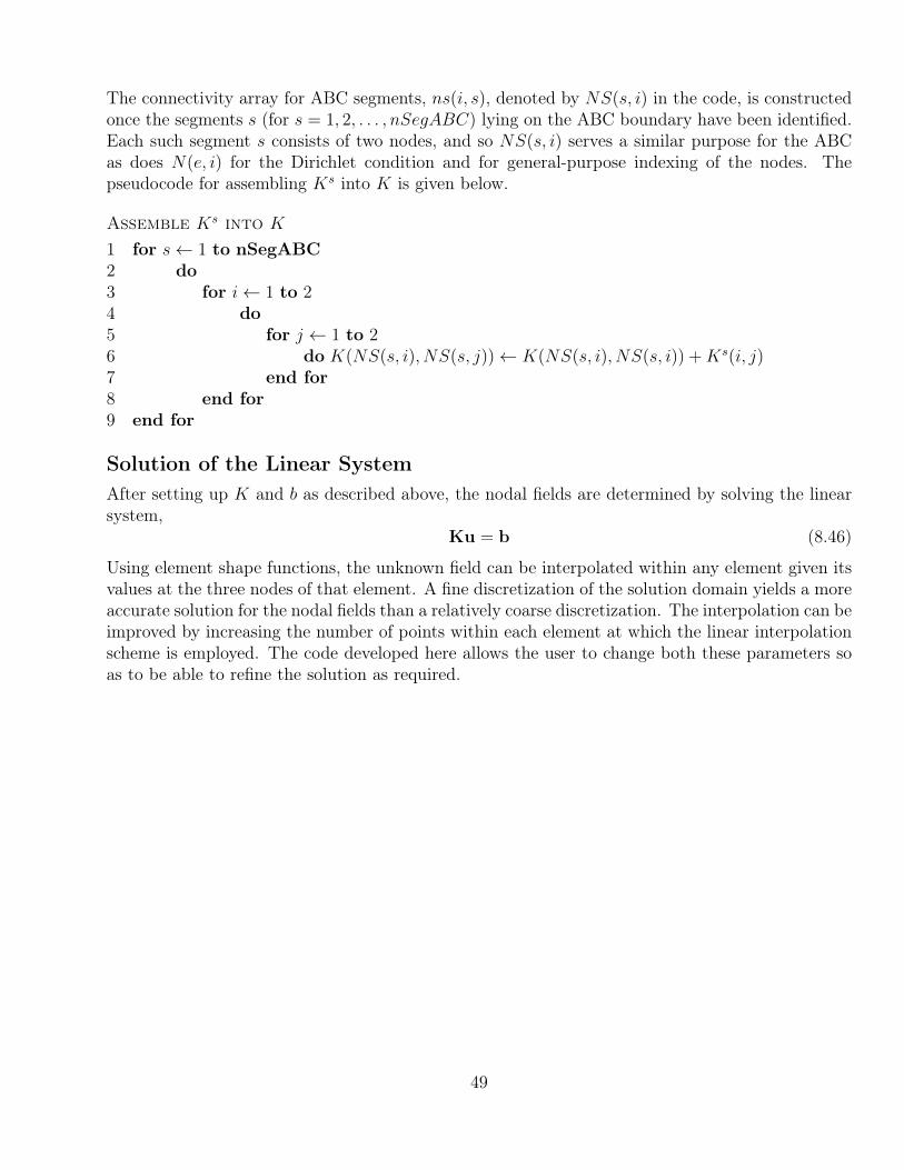
The connectivity array for ABC segments, ns(i, s), denoted by NS(s, i) in the code, is constructedonce the segments s (for s = 1, 2, . . . , nSegABC) lying on the ABC boundary have been identified.Each such segment s consists of two nodes, and so NS(s, i) serves a similar purpose for the ABCas does N(e, i) for the Dirichlet condition and for general-purpose indexing of the nodes. Thepseudocode for assembling Ks into K is given below.

Assemble Ks into K

1 for s← 1 to nSegABC2 do3 for i← 1 to 24 do5 for j ← 1 to 26 do K(NS(s, i), NS(s, j))← K(NS(s, i), NS(s, i)) +Ks(i, j)7 end for8 end for9 end for

Solution of the Linear SystemAfter setting up K and b as described above, the nodal fields are determined by solving the linearsystem,

Ku = b (8.46)

Using element shape functions, the unknown field can be interpolated within any element given itsvalues at the three nodes of that element. A fine discretization of the solution domain yields a moreaccurate solution for the nodal fields than a relatively coarse discretization. The interpolation can beimproved by increasing the number of points within each element at which the linear interpolationscheme is employed. The code developed here allows the user to change both these parameters soas to be able to refine the solution as required.

49

Appendix B: First Order AbsorbingBoundary Condition

The first order Absorbing Boundary condition has the form

∂φsc

∂ρ+

(jk0 +

1

2ρ

)φsc = 0 (8.47)

The mixed boundary condition on a curve Γ2 is given by(αx∂Φ

∂xax + αy

∂Φ

∂yay

)· an + γΦ = q (8.48)

which, in this case, is used to enforce the first order absorbing boundary condition [3], given by

∂Φsc

∂ρ+

(jk0 +

1

2ρ

)Φsc = 0 (8.49)

Here, Φsc is the scattered field. For this problem, Φsc = Escz = Ez −Einc

z . In free space µr = 1, andthe ρ-direction is normal to the outer boundary Γ2 on which the ABC is to be imposed. Therefore,(

∂Ez∂x

ax +∂Ez∂y

ay

)· an =

∂Ez∂ρ

(8.50)

γ = jk0 +1

2ρ(8.51)

q = −jk0Eincz (ax · an) +

(jk0 +

1

2ρ

)Eincz (8.52)

To summarize, a first order ABC on boundary Γ2 can be imposed through the use of themixed boundary condition with the assignment of γ and q according to the above equations.In the program, these boundary conditions are imposed on the discretized solution domain, afterdetermining the connectivity arrays n(e, i) and ns(s, i) [1]. The outer boundary Γ2 is chosen to bea circular boundary with radius ρABC .

In enforcing the ABC, there are three cases to consider for each element e, accordingly as whichone of the three edges lies on the ABC. These cases are listed below, along with the correspondingvalues of pei (for i = 1, 2, 3) that must be assigned. Here lij denotes the length of edge i→ j.

50

Figure 8.2: Case I: Edge 1→ 2 lies on the ABC boundary

Case 1: Edge 1→ 2 lies on the ABC boundary

pe1 = E0q0l12e−jk0xe1

(1− jk0x21 − e−jk0x21

(k0x21)2

)(8.53)

pe2 = E0q0l12e−jk0xe1

(−1 + (jk0x21 + 1)e−jk0x21

(k0x21)2

)(8.54)

pe3 = 0 (8.55)

whereq0 = γ − jk0(ye2 − ye1)

l12

(8.56)

Case 2: Edge 3→ 1 lies on the ABC boundary

pe1 = E0q0l12e−jk0xe3

(−1 + (jk0x13 + 1)e−jk0x13

(k0x13)2

)(8.57)

pe2 = 0 (8.58)

pe3 = E0q0l13e−jk0xe3

(1− jk0x13 − e−jk0x13

(k0x13)2

)(8.59)

whereq0 = γ − jk0(ye1 − ye3)

l13

(8.60)

Case 3: Edge 2→ 3 lies on the ABC boundary

pe1 = 0 (8.61)

pe2 = E0q0l23e−jk0xe2

(1− jk0x32 − e−jk0x32

(k0x32)2

)(8.62)

pe3 = E0q0l12e−jk0xe2

(−1 + (jk0x32 + 1)e−jk0x32

(k0x32)2

)(8.63)

whereq0 = γ − jk0(ye3 − ye2)

l23

(8.64)

In the alternate formulation (8.33− 8.37), the elements of Ks are given by

Ks(i, j) = γls

6(1 + δij) (8.65)

51

Appendix C: Second Order AbsorbingBoundary Condition

In this appendix, the exact details of how the second order ABC is discretized and imposed on acircular boundary, are described.

Let Γ2 denote the surface over which the second order absorbing boundary condition (2-ABC)is to be imposed. The boundary condition of the third kind is given by(

αx∂φ

∂xnx + αy

∂φ

∂yny

)+ γφ = q on Γ2 (8.66)

The absorbing boundary condition must be recast in this canonical form so as to determine theelements of the vector pe (c.f. Appendix A). The 2-ABC is expressible in this form if we split φ asφ = φinc + φsc, that is, as a sum of an incident field and a scattered field, and identify γ and q tobe given by2

γ = α

[jk0 +

κ

2− jκ2

8(jκ− k0)− j

2(jκ− k0)

∂2

∂s2

](8.67)

q = α∂φinc

∂n+ α

[jk0 +

κ

2− jκ2

8(jκ− k0)

]φinc − jα

2(jκ− k0)

∂2φinc

∂s2(8.68)

In order to incorporate the general boundary condition of the third kind, contributions from thefunctional

Fb =

∫Γ2

(1

2φγφ− qφ

)dΓ (8.69)

must be accounted for in the weak form given. Here, γ has been “sandwiched” by the unknown field.This is because γ is self-adjoint, assuming Γ2 to be a smooth closed contour, and is now an operatorrather than a scalar function as it was in case of the first order ABC [1]. To further simplify theanalysis, we write

γ = γ1 + γ2∂2

∂s2(8.70)

with

γ1 = α

[jk0 +

κ

2− jκ2

8(jκ− k0)

](8.71)

γ2 = − jα

2(jκ− k0)(8.72)

2It is assumed hereafter that αx = αy = α.

52

We can write Fb as

Fb =

∫Γ2

[1

2

(γ1φ

2 + γ2φ∂2φ

∂s2

)− qφ

]dΓ (8.73)

=

∫Γ2

[1

2γ1φ

2 − 1

2γ2

(∂φ

∂s

)2

− qφ

]dΓ (8.74)

where integration by parts has been carried out on the second term of equation (8.73), assumingΓ2 is indeed a smooth closed contour. The negative sign here is incorrectly stated as a positive signin Jin [1]. The next step is to discretize Fb over each element as was done for the 1-ABC:

Fb =Ms∑s=1

F sb (φs) (8.75)

where F sb denotes the integral over segment s. Differentiating with respect to φsi gives the matrix

system ∂F s

b

∂φs

= [Ks]φs − bs (8.76)

with the elements in [Ks] and bs given by

Ksij =

∫ 1

0

γN siN

sj lsdξ i, j = 1, 2 (8.77)

bsi =

∫ 1

0

qN si lsdξ i = 1, 2 (8.78)

with q given by (6.69). For the 2-ABC, the expression for Ksij is given by

Ksij =

∫ 1

0

(γ1l

sN siN

sj −

γ2

ls∂N s

i

∂ξ

∂N sj

∂ξ

)dξ (8.79)

Here N s1 (ξ) = 1− ξ and N s

2 (ξ) = ξ, so that N s1 (ξ) +N s

2 (ξ) = 1. This gives us

Ks11 = Ks

22 = γs1ls

3+γs2ls

(8.80)

Ks12 = Ks

21 = γs1ls

6− γs2ls

(8.81)

Evaluation of peiThere are three cases to consider while imposing the 2nd order ABC on a circular boundary, de-pending on which edge of a triangular boundary element lies on the ABC contour. These threecases are similar to those considered in the 1nd order ABC in Appendix B, but the expressions forpei are considerably more complex because of the structure of the function q in (8.68), and the factthat γ is now a differential operator.

53

The unknown field is φ = Ez and φinc = Eincz = E0e

−jk0x. Now, q becomes

q(x, y) = −jk0E0α

ρxe−jk0x+α

[jk0 +

κ

2− jκ2

8(jκ− k0)

]E0e

−jk0x− jα

2(jκ− k0)

(jk0x

ρ2− k2

0y2

ρ

)E0e

−jk0x

(8.82)Since pei involves line integrals of q, we can express the edge along which the line integral is to becomputed through the slope-intercept form of a straight line,

y = mx+ c (8.83)

thereby converting q to a function of x alone along the edge under consideration. For simplification,we define

a = −jk0αE0

ρ(8.84)

b = α

[jk0 +

κ

2− jκ2

8(jκ− k0)

]E0 (8.85)

c1 =αk0E0

2(jκ− k0)ρ2(8.86)

c2 =jαk2

0E0

2(jκ− k0)ρ(8.87)

We assume that ρ is constant over the edge (contour) of integration. This is an approximationbecause ρ is constant only over the circular ABC boundary, not over any edge of the polygon that isthe discretized version of this boundary. Such an approximation was made in case of the 1-ABC aswell. We expect that due to fine graining of the 2-ABC, this approximation will affect its accuracyless than in case of the 1-ABC. However, this approximation is not so poor, because we can increasethe fineness of the mesh, which would decrease the edge length of the approximate polygon andmake it closer to the actual circular boundary. With this assumption, a, b, c1 and c2 are globalconstants and we have

q(x, y) = axe−jk0x + be−jk0x + c1xe−jk0x + c2y

2e−jk0x (8.88)

Further, substituting y = mx+ c, we get

q(x) ≡ A1e−jk0x + A2xe

−jk0x + A3x2e−jk0x (8.89)

where

A1 = b+ c2c2 (8.90)A2 = 2c2cm+ c1 + a (8.91)A3 = c2m

2 (8.92)

Case 1: Edge 1→ 2 lies on the ABC boundary

In this case,

m =y2 − y1

x2 − x1

and c =x1y2 − x2y1

x2 − x1

(8.93)

54

The line can be parametrized as

x = x1 + ξ(x2 − x1) (8.94)y = y1 + ξ(y2 − y1) (8.95)

where ξ ∈ [0, 1]. This allows us to recast q in the form

q(ξ) ≡ (A1 + A2ξ + A3ξ2)e−jk0x21ξ (8.96)

where

A1 = (A1 + A2x1 + A3x21)e−jk0x1 (8.97)

A2 = (A2 + 2A3x1)x21e−jk0x1 (8.98)

A3 = A3x221e−jk0x1 (8.99)

The integrals defining the elements of pe are:

pe1 = −∫ 1

0

(1− ξ)q l12 dξ (8.100)

pe2 = −∫ 1

0

ξ q l12 dξ (8.101)

pe3 = 0 (8.102)

Thus, the elements of pe are:

pe1 =l12

(k0x21)4

[2A3(3− jk0x21) + k0x21

A1k0x21(−1 + jk0x21) + A2(2j + k0x21)

+

e−jk0x21

k0x21(A1k0x21 + A2(−2j + k0x21)) + A3(−6 + k0x21(−4j + k0x21))

]pe2 = − l12

(k0x21)4

[6A3 + k0x21(2jA2 − A1k0x21) +

e−jk0x21

−6A3 − 2j(A2 + 3A3)k0x21 + (A1 + 2A2 + 3A3)k2

0x221 + j(A1 + A2 + A3)k3

0x321

]pe3 = 0

where xij = xi − xj. If x21 = 0, we can write

q(y) = q1 + q2y2 (8.103)

where

q1 = axe−jk0x1 + be−jk0x1 + c1x1e−jk0x1 (8.104)

q2 = c2e−jk0x1 (8.105)

55

In this case, the elements of pe become

pe1 = −l12

∫ 1

0

(1− ξ)(q1 + q2(y1 + ξ(y2 − y1))2)dξ

= l12

[−q1

2− q2y

21

4− q2y1y2

6− q2y

22

12

]pe2 = −l12

∫ 1

0

ξ(q1 + q2(y1 + ξ(y2 − y1))2)dξ

= l12

[−q1

2− q2y

21

12− q2y1y2

6− q2y

22

4

]pe3 = 0

Case 2: Edge 3→ 1 lies on the ABC boundary

In this case, the expressions listed for case 1 above, can be used by making the following transfor-mations:

x1 → x3

x2 → x1

y1 → y3

y2 → y1

l12 → l31

The slope and intercept are given by

m =y1 − y3

x1 − x3

and c =x3y1 − x1y3

x1 − x3

(8.106)

so thatq(ξ) ≡ (A1 + A2ξ + A3ξ

2)e−jk0x13ξ (8.107)

where

A1 = (A1 + A2x3 + A3x23)e−jk0x3 (8.108)

A2 = (A2 + 2A3x3)x13e−jk0x3 (8.109)

A3 = A3x213e−jk0x3 (8.110)

with Ai (i = 1, 2, 3), given by equations (8.97− 8.99) and m and c given by equation (8.106). Theintegrals defining the elements of pe are:

pe1 = −∫ 1

0

ξ q l31 dξ (8.111)

pe2 = 0 (8.112)

pe3 = −∫ 1

0

(1− ξ)q l31 dξ (8.113)

56

Thus, the elements of pe are:

pe1 = − l31

(k0x13)4

[6A3 + k0x13(2jA2 − A1k0x13) +

e−jk0x13

−6A3 − 2j(A2 + 3A3)k0x13 + (A1 + 2A2 + 3A3)k2

0x213 + j(A1 + A2 + A3)k3

0x313

]pe2 = 0

pe3 =l31

(k0x13)4

[2A3(3− jk0x13) + k0x13

A1k0x13(−1 + jk0x13) + A2(2j + k0x13)

+

e−jk0x13

k0x13(A1k0x13 + A2(−2j + k0x13)) + A3(−6 + k0x13(−4j + k0x13))

]If x13 = 0, we can write

q(y) = q1 + q2y2 (8.114)

where

q1 = axe−jk0x3 + be−jk0x3 + c1x3e−jk0x3 (8.115)

q2 = c2e−jk0x3 (8.116)

In this case, the elements of pe become

pe1 = −l31

∫ 1

0

ξ(q1 + q2(y3 + ξ(y1 − y3))2)dξ

= l31

[−q1

2− q2y

23

12− q2y3y1

6− q2y

21

4

]pe2 = 0

pe3 = −l31

∫ 1

0

(1− ξ)(q1 + q2(y3 + ξ(y1 − y3))2)dξ

= l31

[−q1

2− q2y

23

4− q2y3y1

6− q2y

21

12

]Case 3: Edge 2→ 3 lies on the ABC boundary

In this case, the expressions listed for case 1 above, can be used by making the following transfor-mations:

x1 → x2

x2 → x3

y1 → y2

y2 → y3

l12 → l23

The slope and intercept are given by

m =y3 − y2

x3 − x2

and c =x2y3 − x3y2

x3 − x2

(8.117)

57

so thatq(ξ) ≡ (A1 + A2ξ + A3ξ

2)e−jk0x32ξ (8.118)where

A1 = (A1 + A2x2 + A3x22)e−jk0x2 (8.119)

A2 = (A2 + 2A3x2)x32e−jk0x2 (8.120)

A3 = A3x232e−jk0x2 (8.121)

with Ai (i = 1, 2, 3), given by equations (8.97− 8.99) and m and c given by equation (8.117). Theintegrals defining the elements of pe are:

pe1 = 0 (8.122)

pe2 = −∫ 1

0

(1− ξ)q l23 dξ (8.123)

pe3 = −∫ 1

0

ξ q l23 dξ (8.124)

Thus, the elements of pe are:

pe1 = 0

pe2 =l23

(k0x32)4

[2A3(3− jk0x32) + k0x32

A1k0x32(−1 + jk0x32) + A2(2j + k0x32)

+

e−jk0x32

k0x32(A1k0x32 + A2(−2j + k0x32)) + A3(−6 + k0x32(−4j + k0x32))

]pe3 = − l23

(k0x32)4

[6A3 + k0x32(2jA2 − A1k0x32) +

e−jk0x32

−6A3 − 2j(A2 + 3A3)k0x32 + (A1 + 2A2 + 3A3)k2

0x232 + j(A1 + A2 + A3)k3

0x332

]If x32 = 0, we can write

q(y) = q1 + q2y2 (8.125)

where

q1 = axe−jk0x2 + be−jk0x2 + c1x2e−jk0x2 (8.126)

q2 = c2e−jk0x2 (8.127)

In this case, the elements of pe become

pe1 = 0

pe2 = −l23

∫ 1

0

(1− ξ)(q1 + q2(y2 + ξ(y3 − y2))2)dξ

= l23

[−q1

2− q2y

22

4− q2y2y3

6− q2y

23

12

]pe3 = −l23

∫ 1

0

ξ(q1 + q2(y2 + ξ(y3 − y2))2)dξ

= l23

[−q1

2− q2y

22

12− q2y2y3

6− q2y

23

4

]

58

Appendix D: COMSOL Results

Figure 8.3: Scattered Fields from PEC Cylinder in Air: ABC vs PML (Fig. 7.12)59

Figure 8.4: Scattering from Dielectric Cylinder in Air: ABC vs PML (Fig. 7.13)60

Figure 8.5: Scattering from PEC Cylinder buried under Soil (z-component of total field for dry soil(top) and wet soil (bottom).) (Fig. 7.14)

61

Figure 8.6: Scattering from Dielectric Cylinder buried under Soil (z-component of total field fordry soil (top) and wet soil (bottom). (Fig. 7.15)

62

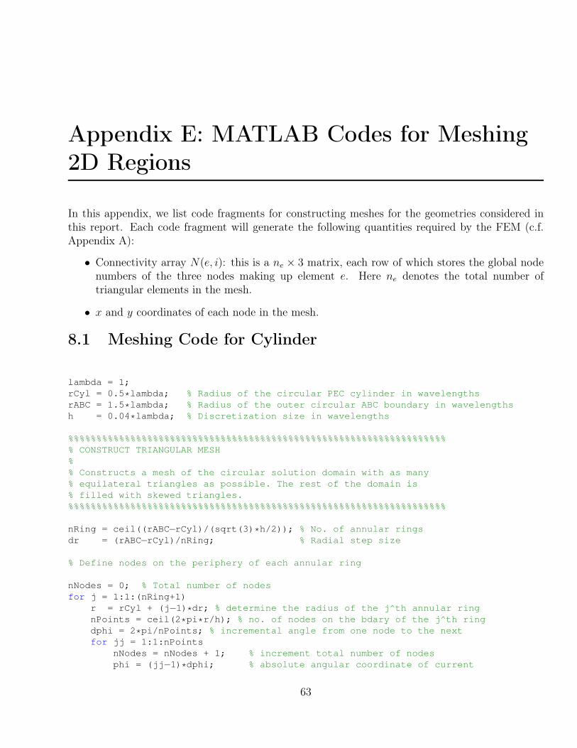
Appendix E: MATLAB Codes for Meshing2D Regions

In this appendix, we list code fragments for constructing meshes for the geometries considered inthis report. Each code fragment will generate the following quantities required by the FEM (c.f.Appendix A):

• Connectivity array N(e, i): this is a ne × 3 matrix, each row of which stores the global nodenumbers of the three nodes making up element e. Here ne denotes the total number oftriangular elements in the mesh.

• x and y coordinates of each node in the mesh.

8.1 Meshing Code for Cylinder

lambda = 1;rCyl = 0.5*lambda; % Radius of the circular PEC cylinder in wavelengthsrABC = 1.5*lambda; % Radius of the outer circular ABC boundary in wavelengthsh = 0.04*lambda; % Discretization size in wavelengths

%%%%%%%%%%%%%%%%%%%%%%%%%%%%%%%%%%%%%%%%%%%%%%%%%%%%%%%%%%%%%%%%%%%% CONSTRUCT TRIANGULAR MESH%% Constructs a mesh of the circular solution domain with as many% equilateral triangles as possible. The rest of the domain is% filled with skewed triangles.%%%%%%%%%%%%%%%%%%%%%%%%%%%%%%%%%%%%%%%%%%%%%%%%%%%%%%%%%%%%%%%%%%%

nRing = ceil((rABC−rCyl)/(sqrt(3)*h/2)); % No. of annular ringsdr = (rABC−rCyl)/nRing; % Radial step size

% Define nodes on the periphery of each annular ring

nNodes = 0; % Total number of nodesfor j = 1:1:(nRing+1)

r = rCyl + (j−1)*dr; % determine the radius of the j^th annular ringnPoints = ceil(2*pi*r/h); % no. of nodes on the bdary of the j^th ringdphi = 2*pi/nPoints; % incremental angle from one node to the nextfor jj = 1:1:nPoints

nNodes = nNodes + 1; % increment total number of nodesphi = (jj−1)*dphi; % absolute angular coordinate of current

63

x(nNodes) = r*cos(phi); % x−coordinate of current nodey(nNodes) = r*sin(phi); % y−coordinate of current node

endend

% Triangulate using Delaunay Triangulationtri = delaunay(x, y);

% At this point, triplot(tri,x,y) shows that the region within the PEC% has also been meshed, so we must eliminate the triangles in this region.

% Eliminate triangles within PECnElements = 0; % No of elements

% length(tri) = size(tri,1) = number of elements% (before removal of elements interior to PEC)for j = 1:1:length(tri)

rem = 0;for jj = 1:1:3

r0 = sqrt(x(tri(j,jj))^2 + y(tri(j,jj))^2); % determine radius of ptif (abs(rCyl − r0) < 0.0001*rCyl) % check for interioricity

rem = rem + 1;end

endif (rem ≤ 2)

nElements = nElements + 1; % increment number of (valid) elementsN(nElements,:) = tri(j,:); % element connectivity array n(e, i)

endend

% N(e, i) is the connectivity array% The global node coordinates are stored in x and y% To access the global node coordinates of node i of element e, use% X = x(N(e,i)), Y = y(N(e,i))

% Delaunay Triangulation does not order nodes in a CCW orientation as% required by the FEM algorithm. So, we have to reorient the local% node numbering. The criterion is that if a triangle has a negative area% computed using the expression for area when the nodes are CCW oriented,% then the nodes must be re−numbered.

for e=1:1:nElementsx21 = x(N(e,2)) − x(N(e,1));x31 = x(N(e,3)) − x(N(e,1));y21 = y(N(e,2)) − y(N(e,1));y31 = y(N(e,3)) − y(N(e,1));Ae = 0.5*(x21*y31 − x31*y21);if Ae < 0

% simple swap of node numberstemp = N(e, 2);N(e, 2) = N(e, 3);N(e, 3) = temp;

endend

64

% Plot the meshfigure;triplot(N, x, y);title('Mesh');xlabel('x (wavelengths)');ylabel('y (wavelengths)');axis([−rABC rABC −rABC rABC]);axis square;

8.2 Meshing Code for Off-center Cylinder

rABC = 1.5; % radius of ABC boundary (in wavelengths)rCyl = 0.5; % radius of cylinder (in wavelengths)cx = 0; % x−coordinate of center of cylindercy = 0.5; % y−coordinate of center of cylinderh = 0.04; % discretization size (in wavelengths)

% Define geometry in distmeshfs = sprintf('ddiff(dircle(p,0,0,%f),dcircle(p,%f,%f,%f))',rABC,cx,cy,rCyl);fd = inline(fs,'p');box=[−rABC,−rABC;rABC,rABC];[p,N]=distmesh2d(fd,@huniform,h,box,[]); % call distmesh[p,N]=fixmesh(p,N); % remove multiple points

% Delaunay Triangulation does not order nodes in a CCW orientation as% required by the FEM algorithm. So, we have to reorient the local% node numbering. The criterion is that if a triangle has a negative area% computed using the expression for area when the nodes are CCW oriented,% then the nodes must be re−numbered.

for e=1:1:nElementsx21 = x(N(e,2)) − x(N(e,1));x31 = x(N(e,3)) − x(N(e,1));y21 = y(N(e,2)) − y(N(e,1));y31 = y(N(e,3)) − y(N(e,1));Ae = 0.5*(x21*y31 − x31*y21);if Ae < 0

% simple swap of node numberstemp = N(e, 2);N(e, 2) = N(e, 3);N(e, 3) = temp;

endend

8.3 Meshing Code for Square Object

clear fem; % Clear fem object (previously stored, if any)

rABC = 1.5; % radius of ABC boundary (in wavelengths)

65

aSq = 0.5; % side of square (in wavelengths)h = 0.04; % discretization size (in wavelengths)% Define geometry in comsolfem.geom=circ2(rABC)−rotate(rect2(sSq,aSq),0);fem.mesh=meshinit(fem,'hmax',h);figure,meshplot(fem);axis([−rABC rABC −rABC rABC]);axis square;

% Extract connectivity matrix and vertex coordianates from COMSOL's% data structureel = get(fem.mesh,'el');N = el3.elem'; % connectivity matrixpt = get(fem.mesh,'p');p = pt';x = p(:,1); % x coordinatesy = p(:,2); % y coordinates

% Delaunay Triangulation does not order nodes in a CCW orientation as% required by the FEM algorithm. So, we have to reorient the local% node numbering. The criterion is that if a triangle has a negative area% computed using the expression for area when the nodes are CCW oriented,% then the nodes must be re−numbered.

for e=1:1:nElementsx21 = x(N(e,2)) − x(N(e,1));x31 = x(N(e,3)) − x(N(e,1));y21 = y(N(e,2)) − y(N(e,1));y31 = y(N(e,3)) − y(N(e,1));Ae = 0.5*(x21*y31 − x31*y21);if Ae < 0

% simple swap of node numberstemp = N(e, 2);N(e, 2) = N(e, 3);N(e, 3) = temp;

endend

8.4 Meshing Code for Concave Object

clear fem; % Clear fem object (previously stored, if any)

rABC = 1.5; % radius of ABC boundary (in wavelengths)h = 0.04; % discretization size (in wavelengths)% Define geometry in comsolfem.geom = circ2(rABC) − arc2(0.2,0,0.2,0.5,pi,pi/3,5*pi/3);fem.mesh = meshinit(fem,'hmax',h);figure,meshplot(fem);axis([−rABC rABC −rABC rABC]);axis square;

66

% Extract connectivity matrix and vertex coordianates from COMSOL's% data structureel = get(fem.mesh,'el');N = el3.elem'; % connectivity matrixpt = get(fem.mesh,'p');p = pt';x = p(:,1); % x coordinatesy = p(:,2); % y coordinates

% Delaunay Triangulation does not order nodes in a CCW orientation as% required by the FEM algorithm. So, we have to reorient the local% node numbering. The criterion is that if a triangle has a negative area% computed using the expression for area when the nodes are CCW oriented,% then the nodes must be re−numbered.

for e=1:1:nElementsx21 = x(N(e,2)) − x(N(e,1));x31 = x(N(e,3)) − x(N(e,1));y21 = y(N(e,2)) − y(N(e,1));y31 = y(N(e,3)) − y(N(e,1));Ae = 0.5*(x21*y31 − x31*y21);if Ae < 0

% simple swap of node numberstemp = N(e, 2);N(e, 2) = N(e, 3);N(e, 3) = temp;

endend

8.5 Meshing Code for Two Objects

clear fem; % Clear fem object (previously stored, if any)

rABC = 1.5; % radius of ABC boundary (in wavelengths)aSq = 0.5; % side of square (in wavelengths)h = 0.04; % discretization size (in wavelengths)% Define geometry in comsolfem.geom=circ2(rABC)−arc2(0.1,0.8,0.1,0.3,pi,pi/3,5*pi/3)−rotate(rect2(0.2,0.2),3*pi/2);fem.mesh=meshinit(fem,'hmax',h);figure,meshplot(fem);axis([−rABC rABC −rABC rABC]);axis square;

% Extract connectivity matrix and vertex coordianates from COMSOL's% data structureel = get(fem.mesh,'el');N = el3.elem'; % connectivity matrixpt = get(fem.mesh,'p');p = pt';x = p(:,1); % x coordinatesy = p(:,2); % y coordinates

67

% Delaunay Triangulation does not order nodes in a CCW orientation as% required by the FEM algorithm. So, we have to reorient the local% node numbering. The criterion is that if a triangle has a negative area% computed using the expression for area when the nodes are CCW oriented,% then the nodes must be re−numbered.

for e=1:1:nElementsx21 = x(N(e,2)) − x(N(e,1));x31 = x(N(e,3)) − x(N(e,1));y21 = y(N(e,2)) − y(N(e,1));y31 = y(N(e,3)) − y(N(e,1));Ae = 0.5*(x21*y31 − x31*y21);if Ae < 0

% simple swap of node numberstemp = N(e, 2);N(e, 2) = N(e, 3);N(e, 3) = temp;

endend

68

Appendix F: MATLAB FEM Codes

The code fragement in this section is to be executed after one of the meshing codes in Appendix Dhas been executed, so that the mesh is well defined.

8.6 First Order ABC

% This program solves for the total electric field in a region bounded% by a circular boundary, using the Nodal 2D Finite Element Method.% The 1st order ABC is imposed on the boundary.

% It is assumed on entering this code that the mesh is well defined and% p(:,1) = x−coordinates of vertices% p(:,2) = y−coordinates of vertices% N = node connectivity matrix (properly ordered)

% Define x and y coordinate vectors for use belowx = p(:,1);y = p(:,2);

% Lets find boundary edgesbe = boundedges(p,N);hold on;for i=1:length(be)

x1=x(be(i,1)); x2=x(be(i,2));y1=y(be(i,1)); y2=y(be(i,2));line([x1 x2],[y1 y2],'Color','b','LineWidth',1.5); % Plot the boundary edges

end

nDBC = 0; % no of Dirichlet Boundary Condition nodesnABC = 0; % no of ABC nodesnInt = 0; % no of internal nodesnNodes=length(p); % total no of nodesDBC(1) = 0;% Determine the ABC and DBC nodesfor jj=1:1:nNodes

r0 = sqrt(x(jj)^2+y(jj)^2);if(abs(rABC−r0)<0.0001*rABC) % ABC will be imposed on a circle always

nABC=nABC+1;ABC(nABC)=jj;

else % either an internal node or a node on the object (scatterer)% if jj is an element of the be (bound edges) array% then it is a node on the object hence a DBC node

69

% otherwise it is an internal nodeindex=ArrSearch(be,jj);if(index 6= −1) % DBC node

nDBC=nDBC+1;DBC(nDBC)=jj;

else % internal nodenInt=nInt+1;INT(nInt)=jj;

endend

end

% flag each node% flag = 1 for ABC node% = 0 for internal node% = −1 for DBC nodeflag = zeros(nElements,3);for e=1:nElements

for i=1:3index=ArrSearch(ABC,N(e,i));if (index 6= −1)

flag(e,i) = 1; % ABC nodeelse

index=ArrSearch(DBC,N(e,i));if(index 6= −1)

flag(e,i) = −1; % DBC nodeelse

flag(e,i) = 0; % internal nodeend

endend

end

% Create NS(s,i) array

nSegABC = 0;for e=1:1:nElements

if flag(e,1) == 1 && flag(e,2) == 1nSegABC = nSegABC + 1;NS(nSegABC, 1) = N(e,1);NS(nSegABC, 2) = N(e,2);

elseif flag(e,1) == 1 && flag(e,3) == 1nSegABC = nSegABC + 1;NS(nSegABC, 1) = N(e,1);NS(nSegABC, 2) = N(e,3);

elseif flag(e,2) == 1 && flag(e,3) == 1nSegABC = nSegABC + 1;NS(nSegABC, 1) = N(e,2);NS(nSegABC, 2) = N(e,3);

endend

fprintf(' RESULTS \n\n');

70

fprintf('The number of nodes = %6i\n', nNodes);fprintf('The number of elements = %6i\n', nElements);fprintf('The number of nodes on a Dirichlet boundary = %6i\n', nDBC);fprintf('The number of nodes on an ABC boundary = %6i\n', nABC);

%%%%%%%%%%%%%%%%%%%%%%%%%%%%%%%%%%%%%%%%%%%%%%%%%%%%%%%%%%%%%%%%%%%% DEFINE INPUT PARAMETERS%%%%%%%%%%%%%%%%%%%%%%%%%%%%%%%%%%%%%%%%%%%%%%%%%%%%%%%%%%%%%%%%%%%

lambda = 1;rABC = 1.5*lambda; % Radius of the outer circular ABC boundary in wavelengthsh = 0.04*lambda; % Discretization size in wavelengthsE_0 = 1; % Amplitude of incident electric field (V/m)

%%%%%%%%%%%%%%%%%%%%%%%%%%%%%%%%%%%%%%%%%%%%%%%%%%%%%%%%%%%%%%%%%%%%%%%% DEFINE CONSTANTS FOR EACH ELEMENT%%%%%%%%%%%%%%%%%%%%%%%%%%%%%%%%%%%%%%%%%%%%%%%%%%%%%%%%%%%%%%%%%%%%%%%

J = complex(0.,1.);mur = 1; % Relative permeability (assuming vaccum)epsr = 1; % Relative permittivity (asumming vacuum)k_0 = 2*pi/lambda; % wavenumberalpha = −1/mur;kappa = 1/rABC;gamma_1 = alpha*(J*k_0 + kappa/2 − J*kappa^2/(8*(J*kappa−k_0)));

mu_r = zeros(1,nElements); % relative permeabilityeps_r = zeros(1,nElements); % relative permittivityalpha_x = zeros(1,nElements); % coefficient of second order x term in PDEalpha_y = zeros(1,nElements); % coefficient of second order y term in PDEbeta = zeros(1,nElements); % coefficient of term linear in field in PDEA = zeros(1,nElements); % area of element e

for e=1:1:nElementsmu_r(e) = mur;eps_r(e) = epsr;alpha_x(e) = −1/mur;alpha_y(e) = −1/mur;beta(e) = (k_0)*(k_0)*eps_r(e);

end

% Initialize global K matrix and the right hand side vector bKglobal = zeros(nNodes, nNodes);btilde = zeros(nNodes, 1);

%%%%%%%%%%%%%%%%%%%%%%%%%%%%%%%%%%%%%%%%%%%%%%%%%%%%%%%%%%%%%%%%%%%%%%%% FORMATION OF ELEMENT MATRICES AND ASSEMBLY%%%%%%%%%%%%%%%%%%%%%%%%%%%%%%%%%%%%%%%%%%%%%%%%%%%%%%%%%%%%%%%%%%%%%%%

% coefficients of the linear interpolation functionsa = zeros(nElements,3);b = zeros(nElements,3);c = zeros(nElements,3);

71

be_tilde=zeros(1,nElements);Klocal=zeros(nElements,3,3);

for e=1:1:nElementsx_21 = x(N(e,2)) − x(N(e,1));x_31 = x(N(e,3)) − x(N(e,1));x_32 = x(N(e,3)) − x(N(e,2));x_13 = −x_31;

y_12 = y(N(e,1)) − y(N(e,2));y_21 = −y_12;y_31 = y(N(e,3)) − y(N(e,1));y_23 = y(N(e,2)) − y(N(e,3));

A(e) = 0.5*(x_21*y_31 − x_31*y_21);

x1 = x(N(e,1)); y1 = y(N(e,1));x2 = x(N(e,2)); y2 = y(N(e,2));x3 = x(N(e,3)); y3 = y(N(e,3));

a(e,1) = x2*y3−x3*y2;b(e,1) = y2−y3;c(e,1) = x3−x2;

a(e,2) = x3*y1−x1*y3;b(e,2) = y3−y1;c(e,2) = x1−x3;

a(e,3) = x1*y2−x2*y1;b(e,3) = y1−y2;c(e,3) = x2−x1;

% Evaluate K^e matrix (element K matrix)for i = 1:1:3

for j = 1:1:3if (i == j)

∆ij = 1;else

∆ij = 0;endKlocal(e,i,j) = (alpha_x(e)*b(e,i)*b(e,j)+

alpha_y(e)*c(e,i)*c(e,j))/(4*A(e))+A(e)*beta(e)*(1+∆ij)/12;

endend

% Evaluate b_tilde^e vectorfor i = 1:1:3

fun = @(u,v)betilde(u,v,a(e,i),b(e,i),c(e,i),k_0,x1,x2,x3,y1,y2,y3);% use for scattered field formulation (change eps and% mu for dielectrics, etc.)be_tilde(e,i) = (E_0*k_0*k_0*(1/mu_r(e)−eps_r(e))/(2*A(e)))

72

*dblquad(fun,0,1,0,1);end

end

for e=1:nElements% Assemble K^e into Kglobal and b^e into b

for i = 1:1:3for j = 1:1:3

Kglobal(N(e,i),N(e,j)) = Kglobal(N(e,i),N(e,j)) + Klocal(e,i,j);endbtilde(N(e,i)) = btilde(N(e,i)) + be_tilde(e,i);

endend

% Construct Ks

Ks=zeros(nSegABC,2,2);bs_tilde=zeros(nSegABC,2);for s = 1:1:nSegABC

xdiff = x(NS(s,1)) − x(NS(s,2));ydiff = y(NS(s,1)) − y(NS(s,2));L_s = sqrt(xdiff^2 + ydiff^2);x1 = x(NS(s,1)); x2 = x(NS(s,2));y1 = y(NS(s,1)); y2 = y(NS(s,2));for ii = 1:1:2

fun2 = @(ksi)bstilde1(ksi,ii,alpha,kappa,k_0,x1,x2,L_s,E_0);bs_tilde(s,ii) = quad(fun2,0,1);for jj = 1:1:2

if (ii == jj)Ks(s,ii,jj) = gamma_1*L_s/3;

elseKs(s,ii,jj) = gamma_1*L_s/6;

endend

endend

% Assemble Ks into K

for s = 1:1:nSegABCfor i = 1:1:2

for j = 1:1:2Kglobal(NS(s,i),NS(s,j)) = Kglobal(NS(s,i),NS(s,j)) + Ks(s,i,j);

endend

end

% Assemble bs into b

for s=1:1:nSegABCfor i=1:2

btilde(NS(s,i)) = btilde(NS(s,i)) + bs_tilde(s,i);end

73

end

% Impose Dirichlet Boundary COndition

for i=1:1:nDBCfor j=1:1:nNodes

if (j 6= ABC(i))btilde(j) = btilde(j) − Kglobal(j, DBC(i))*0;

endendKglobal(:,DBC(i)) = 0;Kglobal(DBC(i),:) = 0;Kglobal(DBC(i),DBC(i)) = 1;btilde(DBC(i)) = 0;

end

% Solution of global matrix systemEz = Kglobal\btilde;

% Generate solution over a grid and plot it[xgrid, ygrid] = meshgrid(−rABC:0.01*(2*rABC):rABC, −rABC:0.01*(2*rABC):rABC);Ezgrid = zeros(101,101);

for i = 1:1:101for j = 1:1:101

for e = 1:1:nElements

x2p = x(N(e,2)) − xgrid(i,j);x3p = x(N(e,3)) − xgrid(i,j);y2p = y(N(e,2)) − ygrid(i,j);y3p = y(N(e,3)) − ygrid(i,j);A1 = 0.5*abs(x2p*y3p − x3p*y2p);

x2p = x(N(e,2)) − xgrid(i,j);x1p = x(N(e,1)) − xgrid(i,j);y2p = y(N(e,2)) − ygrid(i,j);y1p = y(N(e,1)) − ygrid(i,j);A2 = 0.5*abs(x2p*y1p − x1p*y2p);

x1p = x(N(e,1)) − xgrid(i,j);x3p = x(N(e,3)) − xgrid(i,j);y1p = y(N(e,1)) − ygrid(i,j);y3p = y(N(e,3)) − ygrid(i,j);A3 = 0.5*abs(x1p*y3p − x3p*y1p);

x21 = x(N(e,2)) − x(N(e,1));x31 = x(N(e,3)) − x(N(e,1));y21 = y(N(e,2)) − y(N(e,1));y31 = y(N(e,3)) − y(N(e,1));Ae = 0.5*abs(x21*y31 − x31*y21);

if abs(Ae−(A1+A2+A3)) < 0.00001*Aeksi = (y31*(xgrid(i,j)−x(N(e,1)))−x31*(ygrid(i,j)−y(N(e,1))))/(2*Ae);ita = (−y21*(xgrid(i,j)−x(N(e,1)))+x21*(ygrid(i,j)−y(N(e,1))))/(2*Ae);

74

N1 = 1 − ksi − ita;N2 = ksi;N3 = ita;Ezgrid(i,j) = N1*Ez(N(e,1)) + N2*Ez(N(e,2)) + N3*Ez(N(e,3));

endend

endend

% Display contour plot of FEM solutionfigure;contourf(xgrid,ygrid,abs(Ezgrid));xlabel('x (wavelengths)');ylabel('y (wavelengths)');axis([−rABC rABC −rABC rABC]);title('Total Electric Field − Contour Plot');axis square;colorbar;

% Evaluate exact solution at rho = (rCyl + rABC)/2

d2p=pi/180;dist=lambda; % where to evaluate the fieldEz_eval=zeros(1,1441);phi=zeros(1,1441);for I=1:1441 %721

phi(I)=(I−1)*0.25; %0.5;xeval=dist*cos(phi(I)*d2p);yeval=dist*sin(phi(I)*d2p);for e=1:nElements

x2p=x(N(e,2))−xeval;x3p=x(N(e,3))−xeval;y2p=y(N(e,2))−yeval;y3p=y(N(e,3))−yeval;A1=0.5*abs(x2p*y3p−x3p*y2p);

x2p=x(N(e,2))−xeval;x1p=x(N(e,1))−xeval;y2p=y(N(e,2))−yeval;y1p=y(N(e,1))−yeval;A2=0.5*abs(x2p*y1p−x1p*y2p);

x1p=x(N(e,1))−xeval;x3p=x(N(e,3))−xeval;y1p=y(N(e,1))−yeval;y3p=y(N(e,3))−yeval;A3=0.5*abs(x1p*y3p−x3p*y1p);

x21=x(N(e,2))−x(N(e,1));x31=x(N(e,3))−x(N(e,1));y21=y(N(e,2))−y(N(e,1));y31=y(N(e,3))−y(N(e,1));Ae=0.5*(x21*y31−x31*y21);

75

if abs(Ae−(A1+A2+A3)) < 0.00001*Aeksi=(y31*(xeval−x(N(e,1)))−x31*(yeval−y(N(e,1))))/(2*Ae);ita=(−y21*(xeval−x(N(e,1)))+x21*(yeval−y(N(e,1))))/(2*Ae);N1=1−ksi−ita;N2=ksi;N3=ita;Ez_eval(I)=N1*Ez(N(e,1))+N2*Ez(N(e,2))+N3*Ez(N(e,3));

endend

end

% Plot the analytical solution and the FEM solution at a distance 'dist'

figure;plot(phi,abs(Ez_eval),'b−−'),legend('FEM (1^st order ABC)');xlabel('Angle (degrees)');ylabel('Electric Field (V/m)');axis([0 360 0 2*E_0]);grid on;

%%%%%%%%%%%%%%%%%%%%%%%%%%%%%%%%%%%%% FUNCTIONS%%%%%%%%%%%%%%%%%%%%%%%%%%%%%%%%%%%%% evaluate bsilde1(e,i) for the FIRST ORDER ABC (1 = FIRST ORDER ABC)%%%%%%%%%%%%%%%%%%%%%%%%%%%%%%%%%%%%function f1 = bstilde1(ksi,m,alpha,kappa,k_0,x1,x2,L_s,E_0)N = ksi;if (m == 1)

N = 1−ksi;endJ = complex(0.,1.);x = (1−ksi).*x1 + ksi.*x2;expfac = exp(−J*k_0.*x);f1 = alpha*(J*k_0 + 0.5*kappa − J*k_0*kappa.*x).*N.*L_s*E_0.*expfac;

%%%%%%%%%%%%%%%%%%%%%%%%%%%%%%%%%%%%% evaluate btilde(e,i)%%%%%%%%%%%%%%%%%%%%%%%%%%%%%%%%%%%%

function f2 = betilde(u,v,a,b,c,k_0,x1,x2,x3,y1,y2,y3)J = complex(0.,1.);x = (1−u).*x1 + u.*((1−v).*x2 + v.*x3);y = (1−u).*y1 + u.*((1−v).*y2 + v.*y3);jacob = (−x1+(1−v).*x2+v.*x3).*(−u.*y2+u.*y3)−

(−y1+(1−v).*y2+v.*y3).*(−u.*x2+u.*x3);f2 = (a+b.*x+c.*y).*exp(−J*k_0.*x).*jacob;

% simple linear array searchfunction index = ArrSearch(arr,val)res = −1;for ii=1:length(arr)

if (arr(ii)==val)res=ii;break;

76

endendindex=res;

8.7 Second Order ABC

% This program solves for the total electric field in a region bounded% by a circular boundary, using the Nodal 2D Finite Element Method.% The 2nd order ABC is imposed on the boundary.

% It is assumed on entering this code that the mesh is well defined and% p(:,1) = x−coordinates of vertices% p(:,2) = y−coordinates of vertices% N = node connectivity matrix (properly ordered)

% Define x and y coordinate vectors for use belowx = p(:,1);y = p(:,2);

% Lets find boundary edgesbe = boundedges(p,N);hold on;for i=1:length(be)

x1=x(be(i,1)); x2=x(be(i,2));y1=y(be(i,1)); y2=y(be(i,2));line([x1 x2],[y1 y2],'Color','b','LineWidth',1.5); % Plot the boundary edges

end

nDBC = 0; % no of Dirichlet Boundary Condition nodesnABC = 0; % no of ABC nodesnInt = 0; % no of internal nodesnNodes=length(p); % total no of nodesDBC(1) = 0;% Determine the ABC and DBC nodesfor jj=1:1:nNodes

r0 = sqrt(x(jj)^2+y(jj)^2);if(abs(rABC−r0)<0.0001*rABC) % ABC will be imposed on a circle always

nABC=nABC+1;ABC(nABC)=jj;

else % either an internal node or a node on the object (scatterer)% if jj is an element of the be (bound edges) array% then it is a node on the object hence a DBC node% otherwise it is an internal nodeindex=ArrSearch(be,jj);if(index 6= −1) % DBC node

nDBC=nDBC+1;DBC(nDBC)=jj;

else % internal nodenInt=nInt+1;INT(nInt)=jj;

endend

77

end

% flag each node% flag = 1 for ABC node% = 0 for internal node% = −1 for DBC nodeflag = zeros(nElements,3);for e=1:nElements

for i=1:3index=ArrSearch(ABC,N(e,i));if (index 6= −1)

flag(e,i) = 1; % ABC nodeelse

index=ArrSearch(DBC,N(e,i));if(index 6= −1)

flag(e,i) = −1; % DBC nodeelse

flag(e,i) = 0; % internal nodeend

endend

end

% Create NS(s,i) array

nSegABC = 0;for e=1:1:nElements

if flag(e,1) == 1 && flag(e,2) == 1nSegABC = nSegABC + 1;NS(nSegABC, 1) = N(e,1);NS(nSegABC, 2) = N(e,2);

elseif flag(e,1) == 1 && flag(e,3) == 1nSegABC = nSegABC + 1;NS(nSegABC, 1) = N(e,1);NS(nSegABC, 2) = N(e,3);

elseif flag(e,2) == 1 && flag(e,3) == 1nSegABC = nSegABC + 1;NS(nSegABC, 1) = N(e,2);NS(nSegABC, 2) = N(e,3);

endend

fprintf(' RESULTS \n\n');fprintf('The number of nodes = %6i\n', nNodes);fprintf('The number of elements = %6i\n', nElements);fprintf('The number of nodes on a Dirichlet boundary = %6i\n', nDBC);fprintf('The number of nodes on an ABC boundary = %6i\n', nABC);

%%%%%%%%%%%%%%%%%%%%%%%%%%%%%%%%%%%%%%%%%%%%%%%%%%%%%%%%%%%%%%%%%%%% DEFINE INPUT PARAMETERS%%%%%%%%%%%%%%%%%%%%%%%%%%%%%%%%%%%%%%%%%%%%%%%%%%%%%%%%%%%%%%%%%%%

lambda = 1;

78

rABC = 1.5*lambda; % Radius of the outer circular ABC boundary in wavelengthsh = 0.04*lambda; % Discretization size in wavelengthsE_0 = 1; % Amplitude of incident electric field (V/m)

%%%%%%%%%%%%%%%%%%%%%%%%%%%%%%%%%%%%%%%%%%%%%%%%%%%%%%%%%%%%%%%%%%%%%%%% DEFINE CONSTANTS FOR EACH ELEMENT%%%%%%%%%%%%%%%%%%%%%%%%%%%%%%%%%%%%%%%%%%%%%%%%%%%%%%%%%%%%%%%%%%%%%%%

J = complex(0.,1.);mur = 1; % Relative permeability (assuming vaccum)epsr = 1; % Relative permittivity (asumming vacuum)k_0 = 2*pi/lambda; % wavenumberalpha = −1/mur;kappa = 1/rABC;gamma_1 = alpha*(J*k_0 + kappa/2 − J*kappa^2/(8*(J*kappa−k_0)));gamma_2 = −J*alpha/(2*(J*kappa−k_0));

mu_r = zeros(1,nElements); % relative permeabilityeps_r = zeros(1,nElements); % relative permittivityalpha_x = zeros(1,nElements); % coefficient of second order x term in PDEalpha_y = zeros(1,nElements); % coefficient of second order y term in PDEbeta = zeros(1,nElements); % coefficient of term linear in field in PDEA = zeros(1,nElements); % area of element e

for e=1:1:nElementsmu_r(e) = mur;eps_r(e) = epsr;alpha_x(e) = −1/mur;alpha_y(e) = −1/mur;beta(e) = (k_0)*(k_0)*eps_r(e);

end

% Initialize global K matrix and the right hand side vector bKglobal = zeros(nNodes, nNodes);btilde = zeros(nNodes, 1);

%%%%%%%%%%%%%%%%%%%%%%%%%%%%%%%%%%%%%%%%%%%%%%%%%%%%%%%%%%%%%%%%%%%%%%%% FORMATION OF ELEMENT MATRICES AND ASSEMBLY%%%%%%%%%%%%%%%%%%%%%%%%%%%%%%%%%%%%%%%%%%%%%%%%%%%%%%%%%%%%%%%%%%%%%%%

% coefficients of the linear interpolation functionsa = zeros(nElements,3);b = zeros(nElements,3);c = zeros(nElements,3);

be_tilde=zeros(1,nElements);Klocal=zeros(nElements,3,3);

for e=1:1:nElementsx_21 = x(N(e,2)) − x(N(e,1));x_31 = x(N(e,3)) − x(N(e,1));x_32 = x(N(e,3)) − x(N(e,2));x_13 = −x_31;

79

y_12 = y(N(e,1)) − y(N(e,2));y_21 = −y_12;y_31 = y(N(e,3)) − y(N(e,1));y_23 = y(N(e,2)) − y(N(e,3));

A(e) = 0.5*(x_21*y_31 − x_31*y_21);

x1 = x(N(e,1)); y1 = y(N(e,1));x2 = x(N(e,2)); y2 = y(N(e,2));x3 = x(N(e,3)); y3 = y(N(e,3));

a(e,1) = x2*y3−x3*y2;b(e,1) = y2−y3;c(e,1) = x3−x2;

a(e,2) = x3*y1−x1*y3;b(e,2) = y3−y1;c(e,2) = x1−x3;

a(e,3) = x1*y2−x2*y1;b(e,3) = y1−y2;c(e,3) = x2−x1;

% Evaluate K^e matrix (element K matrix)for i = 1:1:3

for j = 1:1:3if (i == j)

∆ij = 1;else

∆ij = 0;endKlocal(e,i,j) = (alpha_x(e)*b(e,i)*b(e,j)+alpha_y(e)*

c(e,i)*c(e,j))/(4*A(e)) + A(e)*beta(e)*(1+∆ij)/12;end

end

% Evaluate b_tilde^e vectorfor i = 1:1:3

fun = @(u,v)betilde(u,v,a(e,i),b(e,i),c(e,i),k_0,x1,x2,x3,y1,y2,y3);% use for scattered field formulation (change eps% and mu for dielectrics, etc.)be_tilde(e,i) = (E_0*k_0*k_0*(1/mu_r(e)−eps_r(e))/(2*A(e)))

*dblquad(fun,0,1,0,1);end

end

for e=1:nElements% Assemble K^e into Kglobal and b^e into b

for i = 1:1:3for j = 1:1:3

Kglobal(N(e,i),N(e,j)) = Kglobal(N(e,i),N(e,j)) + Klocal(e,i,j);

80

endbtilde(N(e,i)) = btilde(N(e,i)) + be_tilde(e,i);

endend

% Construct Ks

Ks=zeros(nSegABC,2,2);bs_tilde=zeros(nSegABC,2);for s = 1:1:nSegABC

xdiff = x(NS(s,1)) − x(NS(s,2));ydiff = y(NS(s,1)) − y(NS(s,2));L_s = sqrt(xdiff^2 + ydiff^2);x1 = x(NS(s,1)); x2 = x(NS(s,2));y1 = y(NS(s,1)); y2 = y(NS(s,2));for ii = 1:1:2

fun2 = @(ksi)bstilde2(ksi,ii,alpha,kappa,k_0,x1,x2,y1,y2,L_s,E_0);bs_tilde(s,ii) = quad(fun2,0,1);for jj = 1:1:2

if (ii == jj)Ks(s,ii,jj) = gamma_1*L_s/3 − gamma_2/L_s;

elseKs(s,ii,jj) = gamma_1*L_s/6 + gamma_2/L_s;

endend

endend

% Assemble Ks into K

for s = 1:1:nSegABCfor i = 1:1:2

for j = 1:1:2Kglobal(NS(s,i),NS(s,j)) = Kglobal(NS(s,i),NS(s,j)) + Ks(s,i,j);

endend

end

% Assemble bs into b

for s=1:1:nSegABCfor i=1:2

btilde(NS(s,i)) = btilde(NS(s,i)) + bs_tilde(s,i);end

end

% Impose Dirichlet Boundary COndition

for i=1:1:nDBCfor j=1:1:nNodes

if (j 6= ABC(i))btilde(j) = btilde(j) − Kglobal(j, DBC(i))*0;

endend

81

Kglobal(:,DBC(i)) = 0;Kglobal(DBC(i),:) = 0;Kglobal(DBC(i),DBC(i)) = 1;btilde(DBC(i)) = 0;

end

% Solution of global matrix systemEz = Kglobal\btilde;

% Generate solution over a grid and plot it[xgrid, ygrid] = meshgrid(−rABC:0.01*(2*rABC):rABC, −rABC:0.01*(2*rABC):rABC);Ezgrid = zeros(101,101);

for i = 1:1:101for j = 1:1:101

for e = 1:1:nElementsx2p = x(N(e,2)) − xgrid(i,j);x3p = x(N(e,3)) − xgrid(i,j);y2p = y(N(e,2)) − ygrid(i,j);y3p = y(N(e,3)) − ygrid(i,j);A1 = 0.5*abs(x2p*y3p − x3p*y2p);

x2p = x(N(e,2)) − xgrid(i,j);x1p = x(N(e,1)) − xgrid(i,j);y2p = y(N(e,2)) − ygrid(i,j);y1p = y(N(e,1)) − ygrid(i,j);A2 = 0.5*abs(x2p*y1p − x1p*y2p);

x1p = x(N(e,1)) − xgrid(i,j);x3p = x(N(e,3)) − xgrid(i,j);y1p = y(N(e,1)) − ygrid(i,j);y3p = y(N(e,3)) − ygrid(i,j);A3 = 0.5*abs(x1p*y3p − x3p*y1p);

x21 = x(N(e,2)) − x(N(e,1));x31 = x(N(e,3)) − x(N(e,1));y21 = y(N(e,2)) − y(N(e,1));y31 = y(N(e,3)) − y(N(e,1));Ae = 0.5*abs(x21*y31 − x31*y21);

if abs(Ae−(A1+A2+A3)) < 0.00001*Aeksi = (y31*(xgrid(i,j)−x(N(e,1)))−x31*(ygrid(i,j)−y(N(e,1))))/(2*Ae);ita = (−y21*(xgrid(i,j)−x(N(e,1)))+x21*(ygrid(i,j)−y(N(e,1))))/(2*Ae);N1 = 1 − ksi − ita;N2 = ksi;N3 = ita;Ezgrid(i,j) = N1*Ez(N(e,1)) + N2*Ez(N(e,2)) + N3*Ez(N(e,3));

endend

endend

% Display contour plot of FEM solutionfigure;

82

contourf(xgrid,ygrid,abs(Ezgrid));xlabel('x (wavelengths)');ylabel('y (wavelengths)');axis([−rABC rABC −rABC rABC]);title('Total Electric Field − Contour Plot');axis square;colorbar;

% Evaluate exact solution at rho = (rCyl + rABC)/2

d2p=pi/180;dist=lambda; % where to evaluate the fieldEz_eval=zeros(1,1441);phi=zeros(1,1441);for I=1:1441 %721

phi(I)=(I−1)*0.25; %0.5;xeval=dist*cos(phi(I)*d2p);yeval=dist*sin(phi(I)*d2p);for e=1:nElements

x2p=x(N(e,2))−xeval;x3p=x(N(e,3))−xeval;y2p=y(N(e,2))−yeval;y3p=y(N(e,3))−yeval;A1=0.5*abs(x2p*y3p−x3p*y2p);

x2p=x(N(e,2))−xeval;x1p=x(N(e,1))−xeval;y2p=y(N(e,2))−yeval;y1p=y(N(e,1))−yeval;A2=0.5*abs(x2p*y1p−x1p*y2p);

x1p=x(N(e,1))−xeval;x3p=x(N(e,3))−xeval;y1p=y(N(e,1))−yeval;y3p=y(N(e,3))−yeval;A3=0.5*abs(x1p*y3p−x3p*y1p);

x21=x(N(e,2))−x(N(e,1));x31=x(N(e,3))−x(N(e,1));y21=y(N(e,2))−y(N(e,1));y31=y(N(e,3))−y(N(e,1));Ae=0.5*(x21*y31−x31*y21);

if abs(Ae−(A1+A2+A3)) < 0.00001*Aeksi=(y31*(xeval−x(N(e,1)))−x31*(yeval−y(N(e,1))))/(2*Ae);ita=(−y21*(xeval−x(N(e,1)))+x21*(yeval−y(N(e,1))))/(2*Ae);N1=1−ksi−ita;N2=ksi;N3=ita;Ez_eval(I)=N1*Ez(N(e,1))+N2*Ez(N(e,2))+N3*Ez(N(e,3));

endend

end

83

% Plot the analytical solution and the FEM solution at a distance 'dist'

figure;plot(phi,abs(Ez_eval),'b−−'),legend('FEM (2^nd order ABC)');xlabel('Angle (degrees)');ylabel('Electric Field (V/m)');axis([0 360 0 2*E_0]);grid on;

%%%%%%%%%%%%%%%%%%%%%%%%%%%%%%%%%%%%% FUNCTIONS%%%%%%%%%%%%%%%%%%%%%%%%%%%%%%%%%%%%% evaluate bsilde2(e,i) for the SECOND ORDER ABC (2 = SECOND ORDER ABC)%%%%%%%%%%%%%%%%%%%%%%%%%%%%%%%%%%%%function f1 = bstilde2(ksi,m,alpha,kappa,k_0,x1,x2,y1,y2,L_s,E_0)N = ksi;if (m == 1)

N = 1−ksi;endJ = complex(0.,1.);x = (1−ksi).*x1 + ksi.*x2;y = (1−ksi).*y1 + ksi.*y2;expfac = exp(−J*k_0.*x);% second order expression for ff1 = alpha*(J*k_0 + 0.5*kappa − J*kappa^2/(8*(J*kappa−k_0))

− J*k_0*kappa.*x −0.5*J*kappa^2/(J*kappa−k_0))*(J*k_0.*x−k_0^2.*y.^2)).*N.*L_s*E_0.*expfac;

%%%%%%%%%%%%%%%%%%%%%%%%%%%%%%%%%%%%% evaluate btilde(e,i)%%%%%%%%%%%%%%%%%%%%%%%%%%%%%%%%%%%%

function f2 = betilde(u,v,a,b,c,k_0,x1,x2,x3,y1,y2,y3)J = complex(0.,1.);x = (1−u).*x1 + u.*((1−v).*x2 + v.*x3);y = (1−u).*y1 + u.*((1−v).*y2 + v.*y3);jacob = (−x1+(1−v).*x2+v.*x3).*(−u.*y2+u.*y3)−

(−y1+(1−v).*y2+v.*y3).*(−u.*x2+u.*x3);f2 = (a+b.*x+c.*y).*exp(−J*k_0.*x).*jacob;

% simple linear array search

function index = ArrSearch(arr,val)res = −1;for ii=1:length(arr)

if (arr(ii)==val)res=ii;break;

endendindex=res;

84