FMU Rep. No. IV-10

(JANUARY 1 9 7 4 )

INDIA METEOROLOGICAL DEPARTMENT

FORECASTING MANUAL

PART IV

COMPREHENSIVE ARTICLES ON SELECTED TOPICS

0 : MOUNTAIN WAVES

BY

R. P. SARKER.

ISSUED BY

THE DEPUTY DIRECTOR GENERAL OF OBSERVATORIES

(FORECASTING)POONA-5

FORECASTING MANUAL REPORTS

No.I-1 Monthly Mean Sea Level Isobaric Charts - R. Ananthakrishnan,

V. Srinivasan and A.R. Ramakrishnan.

No.I-2 Climate of India - Y.P. Rao and K.S. Ramamurti.

Nc.II-1 Methods of Analysis: 1. Map Projections for Heather Charts -

K. Krishna.

No.II-4 Methods of Analysis: 4. Analysis of Hind Field - R.N.Keshava-

murthy.

No.III-1.1 Discussion of Typical Synoptic Weather Situations: Winter -

Western Disturbances and their Associated Features - Y.P.Rao

and V. Srinivasan.Weather

No.III-2.2 Discussion of Typical Synoptic/Situations: Summers Nor'westers

and Andhis and large scale convective activity over Peninsula

and central parts of the country - V. Srinivasan, K.Ramamurthy

and Y.R. Nene.

No.III-3.1 Discussion of Typical Synoptic Weather Situations: Southwest

Monsoon: Active and Weak Monsoon conditions over Gujarat

State - Y.P. Rao, V. Srinivasan, S.Raman and A.R.Ramakrishnan.

No.III-3.2 Discussion of Typical Synoptic Weather Situations: Southwest

Monsoon: Active and Weak Monsoon conditions over Orissa —

Y.P. Rao, V. Srinivasan, A.R.Ramakrishnan and S. Raman.

No.III-3.3 Discussion of Typical Synoptic Weather Situations: Southwest

Monsoons Typical Situations over Northwest India —

M.S.V. Rao, V. Srinivasan and S. Raman.

No.III-3.4 Discussion of Typical Synoptic Weather Situations: Southwest

Monsoons Typical Situations over Madhya Pradesh and Vidarbha -

V. Srinivasan, S.Raman and S. Mukherji.

No.III-3.5 Discussion of Typical Synoptic Weather Situations: Southwest

Monsoons Typical Situations over Uttar Pradesh and Bihar -

V. Srinivasan, S. Raman and S. Mukherji.

No.III-3.6 Discussion of Typical Synoptic Weather Situations: Southwest

Monsoons Typical Situations over West Bengal and Assam and

adjacent States - V. Srinivasan, S. Raman, and S. Mukherji.

No.III-3.7 Discussion of Typical Synoptic Weather Situations: Southwest

Monsoons Typical Situations over Konkan and Coastal Mysore —

V. Srinivasan, S. Raman, S. Mukherji and K. Ramamurthy.

No.III-3.8 Discussion of Typical Synoptic Weather Situations: Southwest

Monsoons Typical Situations over Kerala and Arabian Sea

Islands - V. Srinivasan, S. Mukherji and K. Ramamurthy.

()Contd. on back cover page)

FMU Rep. No.IV - 10

(January 1974)

FORECASTING MANUAL

Part IV - Comprehensive Articles on Selected Topics

10. Mountain Waves

by

R.P. Sarker

Contents

1. Introduction2 . Observational Evidence2.1 Mountain Clouds2.2 Experience of Glider Pi lots2.3 Effects observed from powered a i rc ra f t3 . Flying Aspects of Mountain waves3.1 Vertical currents3.2 Turbulence3.2.1 Turbulence at mountain top level3.2.2 Turbulence above mountain top level3.2.3 Turbulence below mountain top level3.3 Errors in al t imeter readings3.3.1 Graphical Determination of the errors in Altimeter Heights3.4 The effect of the variat ion of horizontal wind speed3.5 The effect on a i rc ra f t icing4. Detecting the Presence of Mountain waves-observational evidence5 . Requirements for Mountain wave formation6. Theoretical works and the i r applications to the prediction of

mountain waves.6.1 Queney's works6.2 Work of Scorer6.2.1 Conditions for occurrence of lee waves6.2.2 Verification of Scorer 's r esu l t s6.3 Works of Palm and Foldvik, Foldvik, Doos, Sarker6.4 Wavelength6.5 The lee wave amplitude

6.5.1 Effect of a succession of ridges

6.5.2 Effect of the profile of air mass stability

6.5.2.1 Inversions

6.5.2.2 Adiabatic lower layer

6.6 Separation of the flow — effect of lee standing eddy

6.6.1 Mountain shape

6.6.2 Stability conditions

6.6.3 Sudden Disturbances

6.7 Short ridges and single peaks

7. Application to Aviation Forecasting

7.1 Observing and Reporting Orographic clouds

7.2 Reports by Pilots

7.3 Application of theoretical and observational results.

Contd.

7.3.1 The likelihood of s ignif icant waves

7 .3 .1 .1 Scale of t e r ra in

7 .3 .1 .2 The presence of Je t streams

7 .3 .1 .3 Irregular Topography7.3.1.4 Changing synoptic conditions7.3.1 .5 Diurnal and Seasonal var iat ions7.3.1.6 Other Effects

7.3.2 Descending current on the lee of a mountain barrier

7.3.3 The level of maximum amplitude

7.3.4 Forecasting Turbulence

7.3.5 Aircraft Icing

8. Some suggested safeguards for flying in Mountain waves

9 . Mountain waves over Western Ghats.

9.1 Mountain waves during Monsoon season

9.2 Some indirect verifications of mountain waves over Western Ghats

9.2.1 Lee waves from cloud observations

9.2.2 Turbulence reports by Aircraft

10. - Mountain waves over Assam-Burma H i l l s .

APPENDIX-A S c a l e for computation of 12

APPENDIX-B Graphical Determinat ion of wave l eng th

REFERENCES

DIAGRAMS.

1. Introduction

In the past, numerous aircraft accidents have occurred over mountains, for

which there was at the time no satisfactory explanation. It has, of course,

long been known that the airflow over mountains or hilly terrain is usually

more disturbed that over flat country. Until recently, however, little was

known concerning the nature and magnitude of disturbances in the airstream caused

by mountain barriers, and the meteorological conditions which have a bearing on

them. In order to make flying over mountains safer, a considerable amount of

research has been conducted in recent years. As a result, much useful informa­

tion has been gathered which, if properly utilised, would be instrumental in

reducing the number of air accidents over mountains.

In particular, it is now known that the influence of mountains on the

airflow is much greater than had been suspected. Indeed, there is circumstan­

tial evidence that under certain meteorological conditions which are not at all

uncommon, the influence of even small hills extends to surprisingly great

heights.

Perhaps the most important information, from the aeronautical view point,

gained in recent years on airflow over mountains, concerns the standing waves,

which under favourable meteorological conditions, form on the lee-side of

mountain barriers. Many past air accidents can now be explained in terms of

these so-called "mountain waves" which, because of the vertical currents they

set up, the severe turbulence they sometimes generate and their effect on the

accuracy of pressure altimeter readings and air navigation, can constitute a

real danger to the unwary pilot.

During the last few years there has grown a considerable body of experi­

mental data on the subject from various sources and notable theoretical

researches into the problem have been carried out, so much so that over at least

an important part of the subject a logical system of ideas has been developed

and can now be presented for the benefit of both forecasters and pilots.

Glider pilots have learnt a great deal of the special air-flow effects which

2

occur in the neighbourhood of mountains. Accordingly much of practical evidence

has come from glider pilots and the potentialities of gliders for research have

been exploited in a number of field investigations. The experiences of the

pilots of powered aircraft, studies of orographic cloud formations as well as

comprehensive programs of observations using the most modern equipment and

techniques have recently rendered a coherent picture on the subject. These

observational data have been supplemented by the recent theoretical studies and

experiments with laboratory models.

In this report an attempt will be made to describe the known properties of

mountain waves with particular reference to their effect on flying conditions.

Methods of detecting and forecasting the occurrence of the mountain waves will

also be discussed together with the measures which should be taken in order

to minimize the inconvenience and hazard of flying over a mountain or hilly

terrain.

In this note it would be desirable to lay more emphasis on the phenomenon

in the Indian regions. But unfortunately, little work has been done on this

problem in India. Most recently only, a few theoretical studies have been

made. No observational data is yet available. We shall, therefore, take

examples from the other parts of the world where data from organised field

studies are available.

Similar notes have been written by Corby (1956) and Alaka (1958).

To start with we shall mention very briefly some of the observational

evidences to make clear the nature of the phenomenon.

2. Observational Evidence

2.1 Mountain clouds

Lenticular clouds are frequently seen over mountainous terrain in all

parts of the world. These clouds remain more or less stationary relative to

the ground and the wind blows through them, so that such clouds are continu­

ally reforming at their up-wind edges and dissipating at the down-wind edges.

3

This has been confirmed by time-lapse photography. On many occasions, specially

to the lee of long ridges, a succession of lenticular clouds, parallel to each

other and to the ridge may be seen; the suggestion that they constitute visible

signs of atmospheric lee waves is very strong.

A similar phenomenon can sometimes be observed when an airstream contain­

ing a layer of stratocumulus crosses a mountainous area. Organized stationary

clearance of the cloud in the form of holes or zones parallel to the lee of

hills or ridges can be seen. The inference is that the clearances are located

when the airstream executes downward undulations associated with topography.

A number of field studies have been carried out aimed at elucidating the

mechanism causing particular cloud formations which are characteristics of

given hills or mountains. Amongst these are the exhaustive study by Manley

(1945) of the Crossfell Helm Wind and its associated clouds and the study by

Kuettner (1939) of the so-called Moazagoti clouds which form over the Riesenge-

birge in Bohemia. Although on different scales, both these phenomena have much

in common and in particular, rotar clouds are commonly observed at levels of

the hill tops, whilst lenticular clouds may also be seen high above the rotor

clouds.

More recently Ludlam (1952) has discussed the formation of orographic cirrus

over the hills of the United Kingdom, and has put forward evidence which supports

his suggestion that a great deal of cirrus forms in atmospheric waves initiated

by topographical features. His observations show that hills in U.K. can produce

waves having sufficient amplitude at 6 km and above to produce cirrus cloud.

According to Stormen (1948) the astonishing mother-of-pearl clouds sometimes seen

high above the Norwegian mountains at 20-25 km also owe their origin to topography.

This has been subsequently theoretically supported by Palm and Foldvik (1960).

Clearly, in the light of such observational evidence, the view that mountains

have no effect on the airflow above more than three times their heights is no

longer tenable.

4

Most recent ly evidence of clouds of orographic origin has come from

s a t e l l i t e cloud photographs and have been reported by Doos (1962), Fr i tz (1965)

Cohen et al (1966). In India, orographic clouds are seen in the Assam and Burma

Hil ls as evidenced from the s a t e l l i t e photographs (De 1970). In the Western

Ghats near the Matheran area, a case of orographic cloud has been reported by

Sinha (1966) from visual observations.

2.2 Experience of Glider Pi lots

In the early days of g l id ing, the sources of ver t ica l motion used were f i r s t

the up-slope motion to be found on the windward side of h i l l s and ridges and l a t e r

thermal up-currents . During the 1930's the pos s ib i l i t i e s of soaring in atmos­

pheric waves began to be explored, special ly in the continent. Numerous ascents

were made on the lee s ide of the Alps in fohn wind conditions and by 1939 several

g l ider ascents to beyond 9 km had been made in the air r i s ing on the up-wind s ide

of wave clouds. The s ignif icant aspect was that many of these ascents were made

well to the lee of the highest ground and could not, therefore, have been simple

cases of f l igh ts in the air stream ascending the windward s lopes. The f i r s t

important ascent by a glider in standing wave in U.K. was made in 1939 by McLean

who reached 3.4 km in the helm wind in Cumberland. On th i s f i r s t occasion,

McLean had d i f f icu l ty in ge t t ing down, and was only able to do so by locating

the down-draught of the wave.

Since the war, wave soaring has become common-place and from the various

reports i t i s found tha t , over the lee ground, waves, i f any, increase in ampli­

tude upwards to some level , above which the waves decrease and eventually die

out . They die away downstream, but a succession of several observable waves

has often been noted in U.K. The order of magnitude of the wave-length is

usually in the range of 2-20 km, but wave-lengths upto 70 km or so are sometimes

observed.

In the spectacular Bishop wave which i s charac te r i s t i c of the airstream

over the Sierra Nevada range in California during winter many ascents to

5

well above 12 km have been made by g l i d e r s . In these wave systems ve r t i ca l

currents of 10 m/sec are common, whilst 20 m/sec has been recorded and i t i s

believed that the ve r t i ca l components exceeding 25 m/sec may occur on occasions.

In addi t ion, turbulence of phenomenal in tens i ty occurs in t h i s area. Field

invest igat ions have been carried out at t h i s location as part of the United

States Mountain Wave Project .

2.3 Effects observed from powered a i rc ra f t

There has been a s teadi ly increasing number of reports of mountain airflow

effects from the p i lo t s of powered a i r c ra f t during the las t few years . This

may be because a i rc ra f t are now flying with increasing regular i ty and frequency

over mountain ranges which l i e across a i r rou tes . The reports confirm tha t

areas of l i f t and sink are commonly to be found over and to the lee of mountains.

Captain D. Mason (1954) of Bri t i sh European Airways Corporation gave a detai led

description of an incident over the mountains of northern Spain on December 18,

a1952 when he was flying viking a i rc ra f t from Madrid to London. He approached

the mountains north of Madrid at 3.4 km and the a i rc ra f t subsequently f e l l to

2.7 km and then rose to 4 .3 km. This was repeated three times in what were un­

doubtedly powerful standing waves. The height changes took place in sp i t e of

his using maximum power in the areas of sink and almost closing the t h r o t t l e s in

the areas of r i s ing a i r . I t can be inferred from th i s that the ve r t i ca l com­

ponents exceeded 2.7 m/sec.

3 . Flying Aspects of Mountain Waves

3.1 Vertical currents

One of the important aspects of mountain waves from the view point of av ia ­

tion i s the ve r t i ca l currents associated with these waves. There may be

updrafts and downdrafts associated with the waves. From the view point of

powered a i rc raf t the low-level downdrafts are most important, since they con­

s t i t u t e one of the principal threa ts to a i r c ra f t safety. Reports from p i lo t s of

powered a i r c r a f t , during the l a s t few years , confirm that ve r t i ca l currents of

6

the order of 5-10 m/sec associated with standing lee-waves are quite common in

various parts of the world. The danger to aircraft from downdrafts of the

above magnitude can be easily appreciated. An aircraft flying more or less

parallel to a ridge might remain in a downdraft continuously until the

whole length of the ridge is traversed. In such circumstances catastrophic

loss of height might occur.

When waves are present, areas of descending currents generally occur

immediately downwind from a mountain ridge. An aircraft flying upwind towards

a mountain ridge, if caught in a strong downdraft near the ridge, might not

be able to regain enough altitude in time to clear the mountain.

The danger to aircraft is enhanced by the fact that flying through waves

is often remarkably smooth even when the rate of lift and sink may be consi­

derable. At night when no warning wave clouds can be seen, or when the sky

is completely overcast, indication of loss of height is given to the pilot

only by the altimeter or the rate of climb indicator, and flying by automatic

pilot can result in disaster to an unwary pilot.

3.2 Turbulence

Pilots have often commented on the extremely smooth flying conditions in

mountain waves, specially in the higher levels. Yet mountain waves also

generate turbulence which can be more violent than any encountered in most

thunderstorms. Of importance to aviation is the fact that the smooth and

turbulent areas are often in close proximity.

Turbulence in mountain waves may occur at, above and below mountain

top level.

3.2.1 Turbulence at mountain top level

The most common and most important seat of severe turbulence in

mountain waves is the area of rotor clouds. The clouds form in standing

eddies under the wave crests at an altitude which is comparable with the

height of the mountain which produces the wave. Measurements made in standing

7

eddies downwind from the Montagne de Lure in France (height 1400 m above

surrounding terrain) have revealed that strong variations in the wind speed ran-

ging from 10 to 25 m/sec occur inside these eddies and that the vertical speeds

can vary from + 8 m/sec to -5 m/sec in 2 or 3 seconds. This is equivalent to a

5

vertical acceleration of 2 to 4 g (Berenger and Gerbier 1946).

Rotor turbulence is much more intense in waves generated by the larger

mountains. Violent sharp-edged gusts exceeding 12 m/sec have been measured in

some Sierra waves, and experienced pilots have reported complete loss of control

of their aircraft for short periods while flying in the rotor areas. According

to Kuettner and Jenkins (1953) high speed aircraft flying with the wind through

such well—developed rotor areas will undergo a breaking effect of such magni­

tude as to endanger the structure of the aircraft.

The danger of rotor turbulence to aviation is accentuated by the fact that

the downdraft in the lee of the rotor and the updraft on the other side of it

can drag an aircraft into the rotor cloud. In a dramatic account of an upwind

flight in a mountain wave, Kuettner and Jenkins describe how their aircraft was

caught in the descending current downwind from the rotor and actually "fell"

into the rotor cloud from above. The buffetting which the aircraft was subjected

to inside the cloud was worse than any the authors had experienced in thunder­

storms.

The most dangerous situation occurs when lack of moisture prevents cloud

formation or when the sky is completely covered by a thick layer of low cloud.

In such cases no prior visual warning is given of the existence of the turbulent

area.

3.2.2 Turbulence above mountain top level

Although exceptionally smooth flying conditions prevail as a rule in moun­

tain waves, this is not invariably the case. Much stronger turbulence has been

experienced in mountain waves over the United States. A report by Harrison(l956)

shows that during the first nine days of 1956, a series of waves occurred down­

wind from the Continental Divide in which severe clear air turbulence was

8

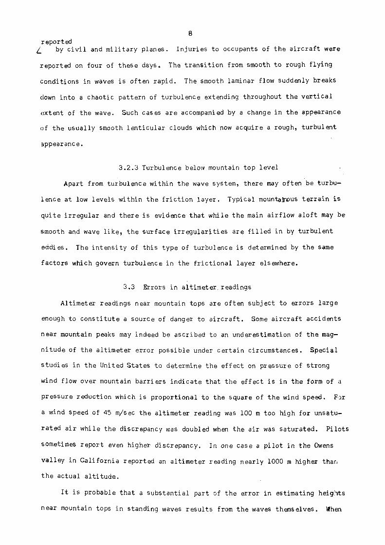
reportedby civil and military planes. Injuries to occupants of the aircraft were

reported on four of these days. The transition from smooth to rough flying

conditions in waves is often rapid. The smooth laminar flow suddenly breaks

clown into a chaotic pattern of turbulence extending throughout the vertical

extent of the wave. Such cases are accompanied by a change in the appearance

of the usually smooth lenticular clouds which now acquire a rough, turbulent

appearance.

3.2.3 Turbulence below mountain top level

Apart from turbulence within the wave system, there may often be turbu­

lence at low levels within the friction layer. Typical mountainous terrain is

quite irregular and there is evidence that while the main airflow aloft may be

smooth and wave like, the surface irregularities are filled in by turbulent

eddies. The intensity of this type of turbulence is determined by the same

factors which govern turbulence in the frictional layer elsewhere.

3.3 Errors in altimeter readings

Altimeter readings near mountain tops are often subject to errors large

enough to constitute a source of danger to aircraft. Some aircraft accidents

near mountain peaks may indeed be ascribed to an underestimation of the mag­

nitude of the altimeter error possible under certain circumstances. Special

studies in the United States to determine the effect on pressure of strong

wind flow over mountain barriers indicate that the effect is in the form of a

pressure reduction which is proportional to the square of the wind speed. For

a wind speed of 45 m/sec the altimeter reading was 100 m too high for unsatu­

rated air while the discrepancy was doubled when the air was saturated. Pilots

sometimes report even higher discrepancy. In one case a pilot in the Owens

valley in California reported an altimeter reading nearly 1000 m higher than

the actual altitude.

It is probable that a substantial part of the error in estimating heights

near mountain tops in standing waves results from the waves themselves. When

9

waves are present, there is generally a zone of descending currents immediately

downstream from the summit and a zone of ascending current farther downstream on

the otherside of the wave. A pilot flying up-wind in the direction of the moun­

tain may take his reading (in the region) where the air is ascending and set his

automatic pilot to conserve his cruising altitude. Almost immediately afterwards,

the aircraft reaches the descending zone where the unwary pilot may lose altitude

at the rate of 500 m/min. or even more. Thus a few minutes after the altimeter

reading is taken, the aircraft may be at an altitude more than 1000 m lower than

that indicated by the instrument.

Although research, in its present stage, gives no clear clue with regard to

the source of errors, we cannot ignore the possibility that large pressure varia­

tions may exist near mountain peaks during high wind. And since these pressure

variations seem always to be in the direction of indicated altimeter heights

which are too high, they constitute an aspect of mountain flying which cannot be

overlooked by pilots.

3.3.1 Graphical Determination of the Errors in Altimeter Heights

In the region of any real atmospheric vortex the meteorological elements

obey very complicated laws. However, under some simplifying assumptions for

mountain top vortices, the following approximate formula may be shown to be true

where po is the pressure in the centre 0 of the vortex, and pA , p and

V are respectively the air pressure, air density and wind velocity at some

point A situated in the region of the vortex. Since the pressure diminishes

towards the centre of the vortex, the difference po - pA characterizes the

drop in atmospheric pressure between the point A and 0. Formula (3.1) shows

that this pressure drop is equal to the product of the density and the square

of the velocity.

It is well—known that very high velocities on the leeside are associated

with the phenomenon of air masses crossing a mountain ridge. In a curved

10

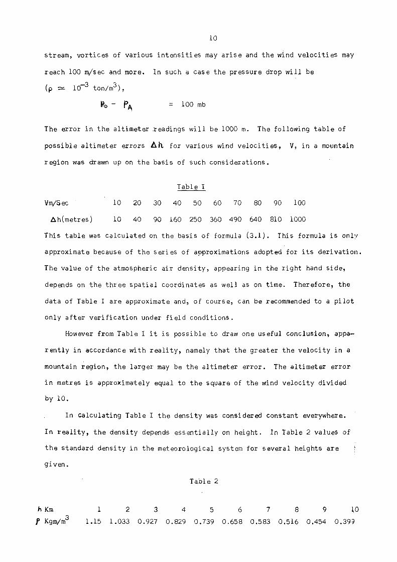
stream, vortices of various intensities may arise and the wind velocities may

reach 100 m/sec and more. In such a case the pressure drop will be

The error in the altimeter readings will be 1000 m. The following table of

possible altimeter errors h for various wind velocities, V, in a mountain

region was drawn up on the basis of such considerations.

Table I

Vm/Sec 10 20 30 40 50 60 70 80 90 100

h(metres) 10 40 90 160 250 360 490 640 810 1000

This table was calculated on the basis of formula (3.1). This formula is only

approximate because of the series of approximations adopted for its derivation.

The value of the atmospheric air density, appearing in the right hand side,

depends on the three spatial coordinates as well as on time. Therefore, the

data of Table I are approximate and, of course, can be recommended to a pilot

only after verification under field conditions.

However from Table I it is possible to draw one useful conclusion, appa­

rently in accordance with reality, namely that the greater the velocity in a

mountain region, the larger may be the altimeter error. The altimeter error

in metres is approximately equal to the square of the wind velocity divided

by 10.

In calculating Table I the density was considered constant everywhere.

In reality, the density depends essentially on height. In Table 2 values of

the standard density in the meteorological system for several heights are

given.

Table 2

h Km 1 2 3 4 5 6 7 8 9 1 0

p Kgm/m3

1.15 1.033 0.927 0.829 0.739 0.658 0.583 0.516 0.454 0.399

11

I t follows from Table 2 that for an increase in the height from 1 to 10 km the

density decreases by almost th ree t imes. But since the error in the al t imeter

readings h depends on the density, the variat ion of the density with height

has to be allowed for in calculat ions of h. Table 3 gives values of h

(in metres) for various heights ,

TABLE - 3

p Kgm/m3

Vm/Secp Kgm/m

3

10 20 30 40 50 60 70 80 90 100

1.15 (h=1 km) 11.5 46 .0 103.0 184.0 287.5 414.0 563.5 736.0 931.5 1150.0

1.03 (h=2 km) 10.3 41 .2 92.7 164.8 257.5 370.8 504.7 659.2 834.3 1030.0

0.93 (h=3 km) 9 . 3 37.2 83.7 148.8 232.5 334.8 455.7 595.2 753.3 930.0

0.83 (h=4 km) 8 . 3 33.2 74.7 132.8 207.5 298.8 406.7 531.2 672.3 830.0

0.74 (h=5 km) 7 . 4 29.6 66.6 118.4 185.0 266.4 362.6 473.6 599.4 740.0

0.66 (h=6 km) 6 . 6 26.4 59.4 105.6 165.0 237.6 323.4 422.4 534.6 660.0

0.58 (h=7 km) 5 . 8 23.2 52.2 92 .8 145.0 208.8 284.2 371.2 469.8 580.0

0.52 (h=8 km) 5 . 2 20 .8 4 6 . 8 83.2 130.0 187.2 254.8 332.8 421.2 520.0

0.45 (h=9 km) 4 . 5 18.0 40.5 72.0 112.5 162.5 220.5 288.0 364.5 450.0

0.40 (h=10 km) 4 . 0 16.0 36.0 64.0 100.0 144.0 196.0 256.0 324.0 400.0

Fig.1 is a nomogram for determining altimeter errors from a known value of the

wind velocity, allowing for density variation with height. The horizontal axis

gives the wind velocity and the vertical axis gives the altimeter error. From the

given density for each height, a curve - a parabola - is constructed by means of

formula 3.1 (Table 3). Thus the family of parabolas is obtained. This nomogram

is quite simple and can be easily used.

Suppose, for example, that the airplane flies at a height of 4 km with a wind

velocity of 50 m/sec. In order to find the possible altimeter setting for this,

it is necessary to find on the horizontal scale the point V = 50 m/sec. At this

point a perpendicular is constructed to intersect the curve corresponding the

12

h = 4 km. Then, drawing a para l le l from th i s point to the horizontal ax i s , we

find that in th is case the al t imeter error may reach 200 m. I t i s seen from the

nomogram that the alt imeter errors should markedly decrease with height, and

for a given wind veloci ty and a given height the error cannot exceed a certain

value. Thus, for a wind velocity V = 60 m/sec the error in the al t imeter

readings at a height of 10 km cannot exceed 150 m whereas at a height of 2 km

t h i s error can be more than 350 m.

I t should be borne in mind that an airplane may lose height when flying in

mountain waves. If the p i lo t takes the alt imeter reading in a region of a

mountain wave cres t and then immediately enters a strong descending current on

the lee of the wave c r e s t , the airplane s t a r t s to lose height rapidly , as if

diving into the trough of the wave. If, for example, the velocity of the des­

cending current i s 12.5 m/ sec . then during one minute the height los t by the

plane should be 750 m. Since such ve loc i t ies (sometimes greater ones) are

encountered not infrequently in a descending current on the lee of a c r e s t ,

the importance of allowing for th i s phenomenon in f l ights over a mountainous

t e r r a in becomes obvious.

3.4 The effect of the variat ion of horizontal wind speed

Mountain waves in the usual sense, i . e . a l ternat ing zones of ascending

currents extending over the barr ier as well as downstream, are primarily caused

by the appearance of an orographic ver t ica l velocity component at the moment of

encounter of the undisturbed flow with the ba r r i e r . But the nature of atmos­

pheric a i r i s such that an air particle i s more easily displaced horizontally

than v e r t i c a l l y . I t i s l ikely that simultaneously with orographic ve r t i ca l

veloci ty component an orographic horizontal velocity component appears at the

moment of encounter of the undisturbed flow with the ba r r i e r . Musaelyan(1960)

by solving equations of hydrothermodynamics found tha t disturbances generated

by mountain bar r ie rs in the horizontal velocity component f ie ld extend in

wave form on both sides of the barr ier (hor izonta l ly) , as well as downstream

13

(Fig.2). There also exist undisturbed surfaces along which the orographic

horizontal velocity component vanishes.

Thus it seems that the mountain waves are not only waves in the vertical

velocity component field, but also superimposed on them and inseparably linked

to them are wave disturbances of the horizontal velocity component. Measurements

of fluctuations in the horizontal wind speed between crest and trough were made

during wave conditions in the lee of the Montagne de Lure by tracking a constant

pressure balloon with radar. The results showed a variation in wind speed from

16 m/sec in the trough of the wave to 26 m/sec in the crest (Berenger and

Gerbier 1956). This variation was associated with a wave amplitude of 1350 m.

There is no doubt stronger fluctuations would accompany more intense waves.

Under wave conditions, an aircraft flying parallel to a large ridge lying

across the wind could be subjected to a horizontal wind materially different from

that prevailing a few kilometres away, and could easily get off the course. If

the wind measured in a wave is used as an average over long distances, the ensuing-

error could amount to many kilometres. Thus, the importance of accurate naviga­

tion over mountains, particularly in cloud at night and when ground clearance is

not large, cannot be overestimated.

3.5 The effect on aircraft icing

The vertical displacement of the air in mountain wave is accompanied by a

fluctuation of the temperature between crest and trough. These fluctuations are

reflected in a corrugation of the 0°C isotherm. Measurements by Berenger and

Gerbier (1956) have revealed that the temperature changes are nearly adiabatic,

and since the waves have their largest amplitudes in layers of atmosphere having

great static stability, the level of the 0ºC isotherm in these layers can be sub­

stantially lower in the wave crests than would be indicated from a radiosonde

ascents made in the same air mass, but in a locality which is undisturbed by

waves. Awareness of this possibility may help in avoiding unexpected ice accre­

tion on the aircraft.

14

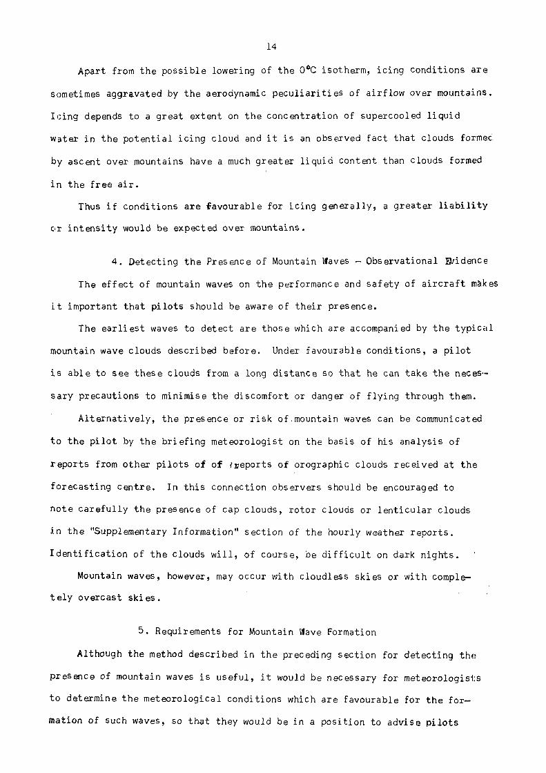
Apart from the possible lowering of the 0ºC isotherm, icing conditions are

sometimes aggravated by the aerodynamic peculiarities of airflow over mountains.

Icing depends to a great extent on the concentration of supercooled liquid

water in the potential icing cloud and it is an observed fact that clouds formec

by ascent over mountains have a much greater liquid content than clouds formed

in the free air.

Thus if conditions are favourable for icing generally, a greater liability

or intensity would be expected over mountains.

4. Detecting the Presence of Mountain Waves - Observational Evidence

The effect of mountain waves on the performance and safety of aircraft makes

it important that pilots should be aware of their presence.

The earliest waves to detect are those which are accompanied by the typical

mountain wave clouds described before. Under favourable conditions, a pilot

is able to see these clouds from a long distance so that he can take the neces­

sary precautions to minimise the discomfort or danger of flying through them.

Alternatively, the presence or risk of mountain waves can be communicated

to the pilot by the briefing meteorologist on the basis of his analysis of

reports from other pilots of of reports of orographic clouds received at the

forecasting centre. In this connection observers should be encouraged to

note carefully the presence of cap clouds, rotor clouds or lenticular clouds

in the "Supplementary Information" section of the hourly weather reports.

Identification of the clouds will, of course, be difficult on dark nights.

Mountain waves, however, may occur with cloudless skies or with comple­

tely overcast skies.

5. Requirements for Mountain Wave Formation

Although the method described in the preceding section for detecting the

presence of mountain waves is useful, it would be necessary for meteorologists

to determine the meteorological conditions which are favourable for the for­

mation of such waves, so that they would be in a position to advise pilots

15

when these conditions are satisfied and waves are likely to occur.

From simple physical reasoning it becomes clear that both static stability

and geostrophic forces are important as restoring forces for the formation of

mountain waves. However, the degree of importance of these factors depends on

the dimensions of the barriers causing the waves. If we consider a very small

hill, a few metres high and not more than 100 m wide, both stability and geostro­

phic forces axe negligible, because on such a scale the atmosphere behaves as

though the lapse rate were adiabatic and the time taken by the air in crossing

the hill is too short to allow the geostrophic forces to come into play. When

the hill is a few kilometres in width, the geostrophic forces remain negligible

whilst stability becomes significant. On an even larger scale as in the case

of the Alps or the Rockies or the Himalayas, for instance, both stability and

geostrophic forces are important.

The requirement of a stable stratification of air mass for wave formation

has been studied by Larson (1954) and Georgii (1956) and others. Besides

stability, another important factor which determines whether the deformation

of anairstream by a mountain ridge is likely to lead to occurrence of standing

waves is the vertical variation of wind. This has been studied in detail by

Forchtgott (1949). Also observations indicate that for standing waves to

occur, the wind speed at some level above the surface must exceed a certain

minimum, which, however, seems to be slightly different in different locali­

ties. This has been studied by Pilsbury (1955), Larson (1954), Jenkins and

Kuettner (1953), Manley (1945) and Colson (1954). However, without going in

detail to these studies, we shall briefly summarise below the results of these

observational studies on the meteorological requirements for the formation of

waves:

(i) Marked stability in the lower layer with comparatively low stability

aloft. The stable layer need not necessarily extend to the ground.

(ii) Wind speed at the level of the summit exceeding a minimum which varies

from about 8 to 13 m/sec depending on the ridge generating the waves, and

16

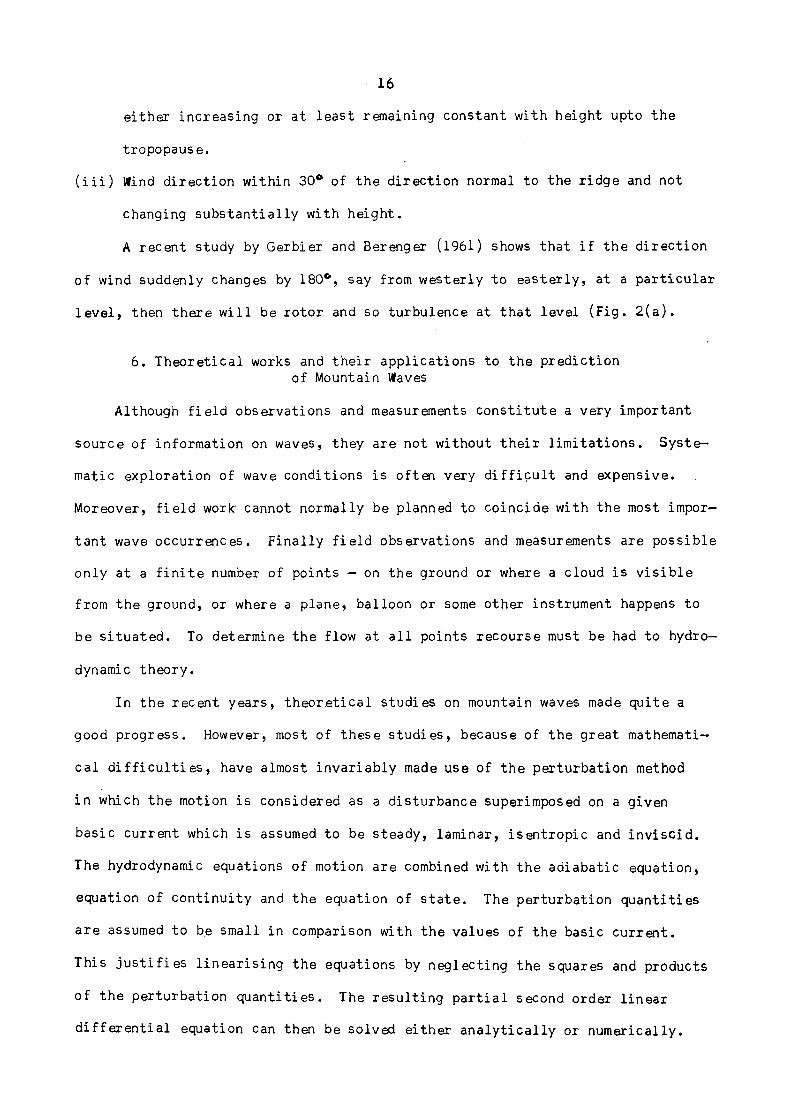
either increasing or at least remaining constant with height upto the

tropopause.

(iii) Wind direction within 30º of the direction normal to the ridge and not

changing substantially with height.

A recent study by Gerbier and Berenger (1961) shows that if the direction

of wind suddenly changes by 180º, say from westerly to easterly, at a particular

level, then there will be rotor and so turbulence at that level (Fig. 2(a).

6. Theoretical works and their applications to the prediction

of Mountain Waves

Although field observations and measurements constitute a very important

source of information on waves, they are not without their limitations. Syste­

matic exploration of wave conditions is often very difficult and expensive.

Moreover, field work cannot normally be planned to coincide with the most impor­

tant wave occurrences. Finally field observations and measurements are possible

only at a finite number of points — on the ground or where a cloud is visible

from the ground, or where a plane, balloon or some other instrument happens to

be situated. To determine the flow at all points recourse must be had to hydro­

dynamic theory.

In the recent years, theoretical studies on mountain waves made quite a

good progress. However, most of these studies, because of the great mathemati­

cal difficulties, have almost invariably made use of the perturbation method

in which the motion is considered as a disturbance superimposed on a given

basic current which is assumed to be steady, laminar, isentropic and inviscid.

The hydrodynamic equations of motion are combined with the adiabatic equation,

equation of continuity and the equation of state. The perturbation quantities

are assumed to be small in comparison with the values of the basic Current.

This justifies linearising the equations by neglecting the squares and products

of the perturbation quantities. The resulting partial second order linear

differential equation can then be solved either analytically or numerically.

17

The limitations of this method are inherent in the assumption underlying

it. The most serious of these are the assumptions of steady, laminar flow and

of small displacement. The restriction to steady laminar flow ignores the fact

that flow over mountains is commonly both unsteady and non-laminar. The assump­

tion of small perturbations restricts the validity of the results to mountains

whose height is small in comparison with their width.

In the following paragraphs we shall give a very brief account of some of

the important theoretical investigations of mountain waves.

6.1 Queney's works

Queney(1947, 48) applied hydrodynamic equations to the flow of a stably

stratified current crossing a mountain. He considered a uniform airstream with

constant static stability and made use of a smooth bell shaped profile for the

mountain. The profile is given by

where is the height of the mountain at z = 0 and b is the maximum height

of the mountain and a is the half-width.

He found that the disturbance pattern varied widely according to the width

of the mountain range. Specifically,

i) If 'a' the half-width of the mountain is of the order of 1 km. there is a

system of short stationary lee waves, or gravity waves,

ii) If 'a' is of the order of 100 km there is a complex system of gravity-

inertia waves. The wave length is of the order of a few hundred kilometres

and the wave amplitude increases upwards. Furthermore, the projection of

the ground streamline on a horizontal plane shows a marked horizontal oscil­

lation.

No wave train is present when the width of the mountain is between the

above two critical values; instead there is only one wave crest and/or trough

on each streamline.

18

6.2 Work of Scorer (1949, 53, 54)

The absence, in Queney's r e s u l t s , of s ta t ionary wave t ra ins in the lee of

mountains for values of ' a ' between 1 and 100 km is at variance with observations

Scorer recognised that th i s unrea l i s t i c resu l t i s due to the assumption of a

uniform airstream. He therefore provided for var iat ion of lapse r a t e and wind

speed along the v e r t i c a l , but confined himself to f r i c t ion le s s , steady laminar

and adiabatic flow over mountain ridges small enough to allow geostrophic forces

to be neglected.

Both s t a b i l i t y and wind figure in a fundamental manner in Scorer 's solu­

t i o n . The relevant parameter i s defined by the expression

where g = acceleration due to gravity

U = horizontal wind component normal to the mountain ridge

z = ver t i ca l co-ordinate posi t ive upwards

θ = potent ial temperature

T = absolute temperature

Y* = adiabatic lapse r a t e

Y = actual lapse r a t e

6.2.1 Conditions for occurrence of lee waves

Scorer found that standing lee waves that are usually observed in prac t ice ,

would be possible only if 12 i s less in some fa i r ly deep upper layer than in

a layer below. This requirement led Scorer to introduce a two layer model

with a value of 12 constant in each layer, but less in the upper than in the

lower layer . There i s a considerable l a t i t ude in the choice of wind and tem-

perature which would sat is fy th i s model, since 12 depends on both the s t a b i ­

l i t y and the wind. Fig.3 gives an example computed by Scorer using the charac­

t e r i s t i c s of wind and temperature shown on the l e f t of the diagram. The lee

19

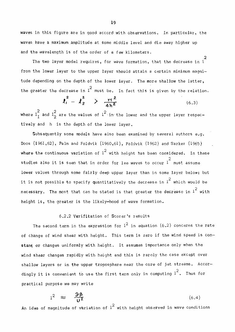
waves in this figure are in good accord with observations. In particular, the

waves have a maximum amplitude at some middle level and die away higher up

and the Wavelength is of the order of a few kilometers.

The two layer model requires, for wave formation, that the decrease in 12

from the lower layer to the upper layer should attain a certain minimum magni­

tude depending on the depth of the lower layer. The more shallow the latter,

the greater the decrease in 12 must be. In fact this is given by the relation.

where and are the values of 12 in the lower and the upper layer respec­

tively and h is the depth of the lower layer.

Subsequently some models have also been examined by several authors e.g.

Doos (1961,62), Palm and Foldvik (1960,61), Foldvik (1962) and Sarker (1965)

where the continuous variation of 12 with height has been considered. In these

studies also it is seen that in order for lee waves to occur 12 must assume

lower values through some fairly deep upper layer than in some layer below; but

i t is not possible to specify quant i ta t ively the decrease in 12 which would be

necessary. The most that can be stated is that greater the decrease in 12 with

height i s , the greater i s the likely-hood of wave formation.

6.2.2 Verification of Scorer 's r esu l t s

The second term in the expression for 12 in equation (6.2) concerns the r a t e

of change of wind shear with height. This term i s zero if the wind speed i s con­

stant or changes uniformly with height. I t assumes importance only when the

wind shear changes rapidly with height and th i s i s rare ly the case except over

shallow layers or in the upper troposphere near the core of j e t streams. Accor-

dingly i t i s convenient to use the f i r s t term only in computing 12 . Thus for

prac t ica l purpose we may wri te

An idea of magnitude of var iat ion of 12 with height observed in wave conditions

20

may be obtained from the study, mentioned by Corby (1957), of 37 reports of marked

waves made by p i lo t s of Br i t i sh European Airways. On the average, the minimum of

12 a lof t was found to be one ninth of the maximum below. This r a t i o i s conf i r ­

med by observations made at St.Auban-Sur-Durance on 25 January 1956 when vigorous

waves occurred on the lee of the Lure Mountain r idge. Conputation of

in th i s case shows that the average value between 1 and 5 km i s about 9 times

tha t between 5 and 10 kms. While the value of one ninth for the decrease in

12 with height should not be used as a quant i ta t ive l imit in forecasting waves,

i t does give an idea of the magnitude of the decrease which is observed during

v/ave s i t u a t i o n s .

6.3 Works of Palm and Foldvik (1960), Foldvik (1962),Doos (1961,62), Sarker (1965)

After Scorer ' s work (1949) with two layer model there were several studies

dividing the atmosphere in two or th ree layers or by numerical computations;

e.g. Palm (1958), Sawyer (1960). The study was then extended by continuous repre -

sentation of the parameter 12 . I t was seen by Palm and Foldvik (1960), Doos

(1961,62) that 12 generally decreases exponentially with increasing height and so

they represented 12 by the form

where fo and λ a re constants . Sarker (1965) found that such a representa-

t ion of 12 i s very sa t i s fac tory in the Western Ghats region during the winter

months, December - March, when the airstream has s tab le s t r a t i f i c a t i o n .

With such a representat ion the ve r t i ca l velocity associated with a wave

of length for a symmetrical mountain p rof i l e given by (6.1)

i s given by

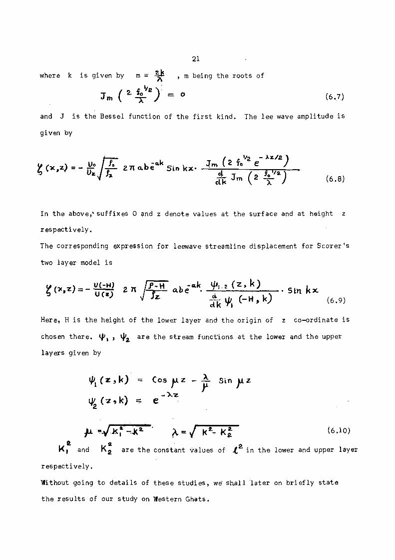
21

where k is given by , m being the roots of

and J i s the Bessel function of the f i r s t kind. The lee wave amplitude i s

given by

In the above, suffixes 0 and z denote values at the surface and at height z

respect ive ly .

The corresponding expression for leewave streamline displacement for Scorer ' s

two layer model i s

Here, H i s the height of the lower layer and the origin of z co-ordinate i s

chosen the re . are the stream functions at the lower and the upper

layers given by

and are the constant values of 2 in the lower and upper layer

respect ive ly .

Without going to de ta i l s of these s tud ies , we shal l l a t e r on brief ly s t a t e

the r e su l t s of our study on Western Ghats.

22

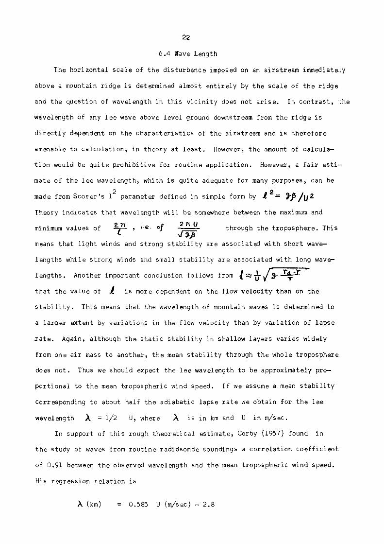
6.4 Wave Length

The horizontal scale of the disturbance imposed on an airstream immediately

above a mountain ridge is determined almost entirely by the scale of the ridge

and the question of wavelength in this vicinity does not arise. In contrast, the

wavelength of any lee wave above level ground downstream from the ridge is

directly dependent on the characteristics of the airstream and is therefore

amenable to calculation, in theory at least. However, the amount of calcula­

tion would be quite prohibitive for routine application. However, a fair esti­

mate of the lee wavelength, which is quite adequate for many purposes, can be

made from Scorer's 12 parameter defined in simple form by

Theory indicates that wavelength will be somewhere between the maximum and

minimum values of through the troposphere. This

means that light winds and strong stability are associated with short wave­

lengths while strong winds and small stability are associated with long wave­

lengths. Another important conclusion follows from

that the value of is more dependent on the flow velocity than on the

stability. This means that the wavelength of mountain waves is determined to

a larger extent by variations in the flow velocity than by variation of lapse

rate. Again, although the static stability in shallow layers varies widely

from one air mass to another, the mean stability through the whole troposphere

does not. Thus we should expect the lee wavelength to be approximately pro­

portional to the mean tropospheric wind speed. If we assume a mean stability

corresponding to about half the adiabatic lapse rate we obtain for the lee

wavelength λ = 1/2 U, where λ is in km and U in m/sec.

In support of this rough theoretical estimate, Corby (1957) found in

the study of waves from routine radiosonde soundings a correlation coefficient

of 0.91 between the observed wavelength and the mean tropospheric wind speed.

His regression relation is

λ (km) = 0.585 U (m/sec) - 2.8

23

This relation is not very far from the approximate theoretical estimate

λ = 1/2 U. Larson (1954) also found in his study of wave clouds that simple

estimates of wavelength obtained by this approach showed good agreement with

observations. As the wavelength is rarely of vital importance in aviation fore­

casting such estimates should suffice when they are required.

From Sarker's (1965) theoretical investigation of mountain waves on the

Western Ghats, there appears to be a suggestion that wavelength increases with

mean tropospheric wind speed. However, as the cases studied were very few, no

relationship of the type given above was possible.

The above wavelength considerations apply to lee wave of the most common

type i.e. those which have their greatest amplitudes in the lower or the middle

troposphere and decrease above. Occasionally lee waves occur with their greatest

amplitude in the upper troposphere or lower stratosphere. Once again the general

wavelength equation cannot be solved rapidly, but by treating the stratosphere

as of infinite stability one obtains an approximate value of the wavelength from

the relations:

where h is the height of the tropopause and is the mean value of 12 for

the troposphere. The above equation appears to be consistent with observations

in that with typical values they suggest much larger wavelengths for this type

of wave, but the relation has not been verified in detail. Although the point

may only rarely be of importance in aviation forecasting, it is appropriate to

mention here that the crest of the first lee wave downstream of a mountain

ridge is commonly observed to be less than one wavelength from the mountain

crest. Indeed for a symmetrical ridge theory indicates that the spacing should

be 3/4 λ .

24

6.5 The lee-wave amplitude

The amplitude of any lee wave is naturally of the greatest importance for

aviation but is unfortunately almost intractable from the forecasting point of

view. This is because, as is evident from equations (6.8) and (6.9) of section

6.3, the amplitude depends in a complex way on both topography as well as on

the properties of the airstream. These aspects were the subject of a theore­

tical study of Corby and Wallington (1956). However, although, it is not yet

possible to predict the lee wave amplitude quantitatively, a knowledge of the

relevant factors governing amplitude is a valuable background information for

a forecaster.

For symmetrical mountain ridges the lee wave amplitude depends on the

height of the ridge above the surrounding countryside and also on the horizontal

scale of the ridge. The dependence on height, viz. proportionality is to be

expected. That is, other things being equal, the higher the mountain, the

greater the amplitude.

The dependence on horizontal scale may be regarded as a resonance effect.

The power spectrum of the mountain cross section necessarily has one or more

concentrations in the vicinity of particular wavelengths (of the usual idea-

lised symmetrical cross-section often adopted in theoretical work there is

of course only one such concentration). If the topography posseses one of th

these maxima near the natural wavelength of the airstream, then the lee wave

amplitude will be much greater than otherwise. Put in another way, we may

Say that if the horizontal scale of the mountain roughly coincides with the

lee wave length, the amplitude will be much larger than for both broader and

narrower mountains. The critical manner in which the amplitude varies with

mountain width is shown by the dashed curve in Fig.4 for an airstream with a

wavelength of 2 km. The curve shows a pronounced maximum when the half

width of the mountain is 1 km and falls off sharply for broader

and narrower ridges. This effect is akin to resonance. The natural wave-

lenath depends on the characteristics of the airstream, but the lee wave

25

amplitude is likely to be small unless the width of the mountain matches the wave­

length of the airstream.

If the height and width are increased in the same proportion, the variation

of the amplitude is that given by the full curve in Fig.4. Thus an airstream

which is favourable for the formation of vigorous waves to the lee of a small

mountain ridge will not necessarily produce bigger waves over larger mountains.

Also the natural wavelength of an airstream increases with the wind speed.

Therefore, larger mountains would require stronger winds for larger amplitude

wave than small mountains. This conclusion is in line with that drawn by

Forchtgott (1949) from his observations in Czechoslovakia.

However, one should be cautious in making use of the above results. For,

most mountainous terrains contain irregularities on a wide range of scales and in

particular, broad mountains often have superposed short wavelength features.

Furthermore, broad mountains may have steep lee slopes and it is of course the

character of the lee slope which is of most importance.

The dependence of lee wave amplitude on the airstream characteristics is

quite complicated. However, this effect can be stated in plain language as

follows. The amplitude of lee waves is subject to wide variations even amongst

airstreams having similar profiles of wind and stability because of the critical

way in which the amplitude depends on the airstream characteristics. Other

things being equal, the largest amplitude lee waves occur when the airstream

satisfies the condition for waves by only a small margin, and in this region

large changes in amplitude may result from small changes in the airstream.

Apart from the question of this sensitive region, it may be said that larger

amplitude waves are theoretically more likely in airstreams containing a

shallow layer of great stability than in conditions of lesser stability through

a deep layer.

A theoretical result which can be exploited in forecasting is concerned

with the amplitude variation of lee waves with height. Generally speaking, the

maximum amplitude is attained in or near the layer of maximum stability. If

26

the stability is concentrated in a shallow layer, as for example, at an inver­

sion, the amplitude has a sharper maximum near this level and falls off

rapidly both above and below. If the stability maximum is diffuse, the varia­

tion of lee wave amplitude with height follows the same pattern but is more

gentle. This result is well supported by observations and enables forecas­

ters to provide useful advice as to the choice of flight level.

6.5.1 Effect of a succession of ridges

A succession of ridges in the direction of the wind may either intensify

or weaken the waves generated, depending on the position of the ridges with

respect to the wavelengths. The influence of the phase of the windward

undulations on the effect which a mountain ridge exerts on an airstream has

been discussed by several investigators. Georgii (1956) has noted that the

best gliding localities for wave soaring have in common a main ridge and a

"counter—ridge" downstream from it at a distance which corresponds nearly to

an exact multiple of wave length. In this manner the wave generated by the

first ridge is reinforced by the counter ridge. This effect may be repeated

several times if there is a succession of ridges so spaced that they are in

harmony with the natural wavelength of the airstream.

6.5.2 Effect of the profile of air mass stability

6.5.2.1 Inversions

It was once thought that the existence of an inversion was essential for

wave formation. This impression might have come from the fact that the

inversions help make the waves visible, since they are usually accompanied by

a concentration of moisture in the layer just beneath them where clouds are

likely to form in the wave crests. However, it is now established from

theory as well as from observations that existence of an inversion is not

essential for the formation of the waves, although, it does play an impor­

tant role in determining the structure and intensity of waves. Corby and

Wallington (1956) have shown that greater amplitudes are possible, if there is

27

considerable static stability through a shallow lower layer than with smaller

stability through a deep layer. The presence of an inversion in the lower layer

would, therefore, be a factor contributing to greater amplitude waves.

The existence of an inversion allows useful conclusions to be drawn with

regard to variation of wave amplitudes with height. In practice the level of

maximum amplitudes is near the level of maximum 12. The presence of an inver­

sion, by concentrating the stability in a shallow layer, brackets the level of

maximum amplitudes within narrow limits and allows its determination with

accuracy. This fact is of considerable importance for aviation. Theory also

indicates that the sharper the inversion, the more pronounced is the maximum wave

amplitude. This means that the intensity of waves will decrease rapidly above

an inversion. This inference is borne out by observation.

6.5.2.2 Adiabatic lower layers

Waves are often observed when the lapse rate near the ground is steep or

even adiabatic. Stability conditions in the lowest layer do affect the structure

of the wave and likelihood of their occurrence. According to Corby and Wallington

(1956) the main effect of an adiabatically mixed layer near the ground is to

reduce the amplitude and increase the wavelength. It, of course, happens parti­

cularly on sunny afternoon, that the adiabatically mixed layer is so deep that

waves cannot exist. In such cases, the stabilisation of the lower layer in the

evening may make conditions favourable for wave formation. This, perhaps,

explains why cirrus clouds are reported more in the mornings and in the evenings

than during daytime and accountS for the fact that after a sunny day glider pilots

soaring over hills often find increasing lift which carries them to heights they

have been unable to attain all the day.

6.6 Separation of the flow-effect of Lee Standing Eddy

However disturbed the flow over mountains may be close to the ground, it is

often remarkably smooth higher up. Timelapse pictures made in connection with

the Sierra Wave Project have shown that the smaller corrugations in the rugged

28

terrain are filled by eddies, while the smooth flow aloft follows the broad

outline of the mountain range. Quite frequently separation occurs, that is,

the lowest smooth streamline leaves the surface completely and reversed flow

sets in.

The importance of separation lies in the fact that it modifies the effec­

tive shape of the mountain. If a mountain is to have its maximum effects, the

low level flow must follow the contours. The presence of a large eddy filling

the space in the lee smooths out the streamline immediately above the mountain

and thus reduces its potential effect on the air flow. When waves are set up,

their phase is such that they generally induce strong flow at the surface down

the lee slope. This fact is confirmed by the curling of the cap cloud down the

lee slope. Conversely, it is sometimes evidenced by the sudden appearance of

waves on the onset of katabatic winds that the descent of air down the lee

slope is favourable for wave formation. It is, therefore, important to know

the factors which have a bearing on separation, particularly that which takes

place near the mountain crest and results in the formation of lee standing

eddy. Scorer (1955) has shown that the following factors play important role

in separation.

6.6.1 Mountain shape

Separation occurs very readily at a sharp edge in the profile of the

ridge. It also occurs more readily when the lee-slope has a precipitous drop

than when it has a smooth and gentle gradient.

6.6.2 Stability Conditions

When the surface is heated anabatic flow is encouraged. Separation is

therefore likely when the lee slope is facing the Sun. On the other hand,

separation is inhibited by differential radiational cooling towards the dusk,

which constrains the wind, to flow down the slope, specially the lee slope.

29

6.6.3 Sudden Disturbances

A downdraft impinging on the lee slope of a mountain range will cause the

air to flow down the slope and may thus prevent separation. Intermittent bursts

of rain with their accompanying downdrafts may thus force the air to flow down

the lee slope and may be instrumental in triggering the occurrence of the waves,

provided the other conditions are favourable.

6.7 Short Ridges and Single Peaks

The results we have described so far apply to two dimensional flow over

long ridges. Flow over short ridges and single peaks presents a problem in

three dimension, for much of the air stream flows round the sides of these obsta­

cles and only the layer in the upper levels goes over the top. Mathematically

the problem is much more difficult than that for the airflow over long ridges.

We must, therefore, rely mainly on observations in order to get the information

concerning the disturbance in the air stream caused by short ridges and single

peaks.

As in the case of stably stratified flow over long ridges, there must be

different types of streaming over short ridges and single peaks. However, no

systematic classification of this type has yet been made. Forchtgott (1951) has

described a type of flow the characteristics of which agree well with some of the

observed occurrences and configuration of clouds in the vicinity of isolated

mountain peaks. Figure 5 illustrates this type of flow. Since most of the air-

stream in the lower layers flows round the sides, there are great horizontal

deflections in the streamlines near the foot of the obstacle, while in the higher

levels the deflections are mainly in the vertical direction. The lower level

streamlines diverge on the windward sides of the hill and return to their original

position in the lee of the obstacle. The lower diagram shows three zones where

whole of the streamlines converge, namely to the and to the left of the

front side and directly to the lee of the obstacle. These are regions where the

vertical component of the wind is upwards. The most marked low level convergence

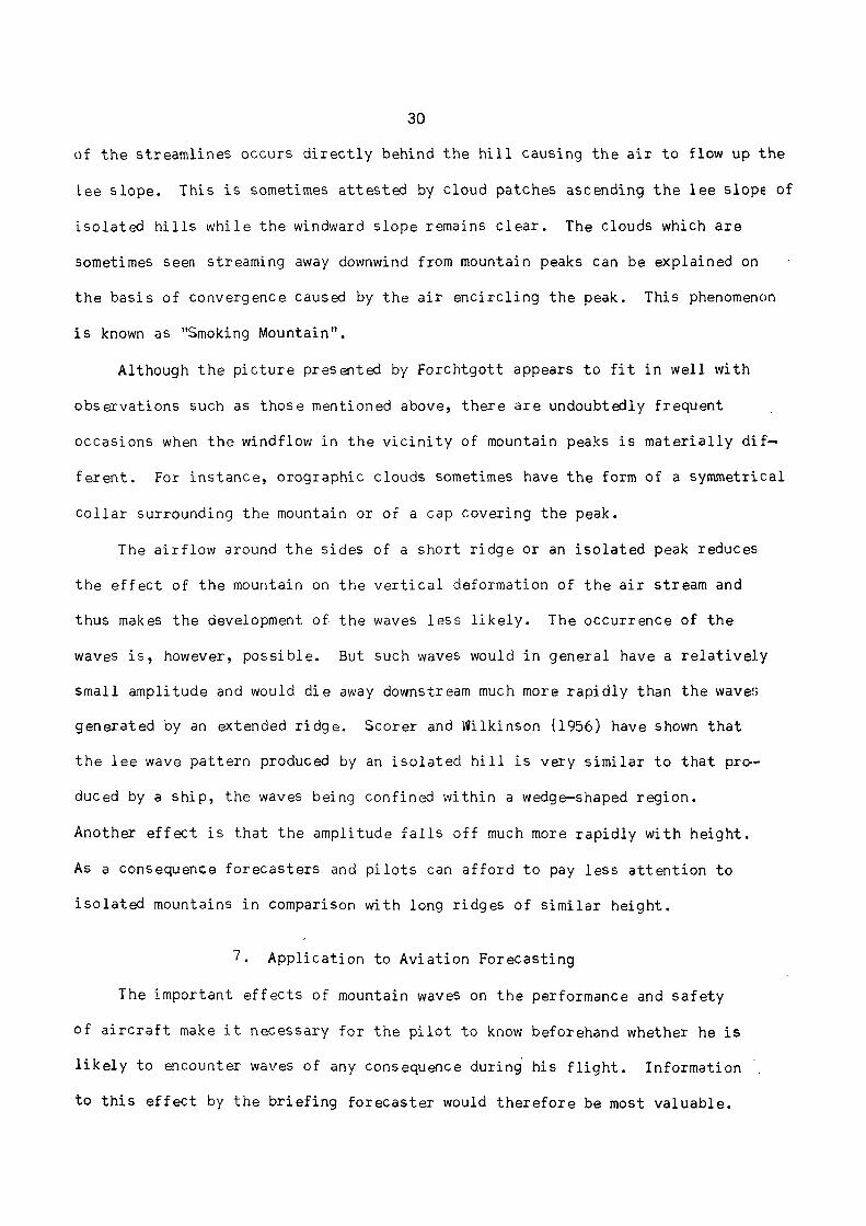
30

of the streamlines occurs directly behind the hill causing the air to flow up the

Lee slope. This is sometimes attested by cloud patches ascending the lee slope of

isolated hills while the windward slope remains clear. The clouds which are

sometimes seen streaming away downwind from mountain peaks can be explained on

the basis of convergence caused by the air encircling the peak. This phenomenon

is known as "Smoking Mountain".

Although the picture presented by Forchtgott appears to fit in well with

observations such as those mentioned above, there are undoubtedly frequent

occasions when the windflow in the vicinity of mountain peaks is materially dif­

ferent. For instance, orographic clouds sometimes have the form of a symmetrical

collar surrounding the mountain or of a cap covering the peak.

The airflow around the sides of a short ridge or an isolated peak reduces

the effect of the mountain on the vertical deformation of the air stream and

thus makes the development of the waves less likely. The occurrence of the

waves is, however, possible. But such waves would in general have a relatively

small amplitude and would die away downstream much more rapidly than the waves

generated by an extended ridge. Scorer and Wilkinson (1956) have shown that

the lee wave pattern produced by an isolated hill is very similar to that pro­

duced by a ship, the waves being confined within a wedge-shaped region.

Another effect is that the amplitude falls off much more rapidly with height.

As a consequence forecasters and pilots can afford to pay less attention to

isolated mountains in comparison with long ridges of similar height.

7. Application to Aviation Forecasting

The important effects of mountain waves on the performance and safety

of aircraft make it necessary for the pilot to know beforehand whether he is

likely to encounter waves of any consequence during his flight. Information

to this effect by the briefing forecaster would therefore be most valuable.

31

7.1 Observing and Reporting Orographic clouds

In attempting to supply this information the forecaster would be greatly

helped by careful reports of clouds which are typical of mountain waves and it

would be advantageous for meteorological service to encourage and train their

observers to detect and report such clouds. Provision for reporting orographic

clouds in the International Cloud Code will also be useful.

7.2 Reports by Pilots

In-flight and post-flight reports by aircraft pilots would also constitute

a helpful source of information to the briefing forecaster. The pilots should

therefore be encouraged to spot and report waves and orographic clouds during

their flight. Even mild waves should be reported, since these waves may inten­

sify by some development in the synopric situation or as a result of the usual

diurnal variation in the lower layer of the airmass.

7.3 Application of Theoretical and Observational Results

Apart from the reports from observers and pilots, the forecaster must

ultimately rely to a great extent on his own analysis of the situation and on

the application of the observational and theoretical results,

7.3.1 The likelihood of significant waves

The first thing to determine is whether standing waves are possible in the

airstream under consideration. This point can be decided by considering the

profile of 12 which should decrease with height if waves are to be possible.

Theoretically, this condition is achieved either by a decrease of stability or

an increase of wind with height. Analysis of numerous cases of waves have

revealed that there is both a substantial increase of wind and a decrease of

stability with height whenever waves are observed. In practice, most situations

favourable for wave development can be identified by an inspection of a repre­

sentative radiosonde ascent in the undisturbed current, without the necessity

for computing the profile of 12. Examples of such ascents made at Stormway

32

and Liverpool on 11th March 1953 are given in Fig. 6(a) and 6(b), in which the

marked stability between 900 and 800 mb and the substantial increase of wind

with height are seen clearly. The computed profiles of 12 are shown for com-

parison in figures 7(a) and 7(b) which show pronounced maxima of 1 around

800-900 mb with much smaller values higher up.

Confirmation that the airstream sampled by the above two soundings was

favourable for waves was provided by an aircraft flying in the same airmass at

a mean height of about 1700 m on the morning of the same day, which passed

through about six smooth waves giving up and down currents of the order of

3.5 m/sec.

In marked contrast, another sounding is given in Figure 8(a), where the

wind speed decreases with height between 800 and 650 mb and which features no

2deep stable layer in the lower troposphere. The corresponding 1 profile given

in figure 8(b) does not show its decrease with height. No wave was observed

in the airstream sampled by this sounding.

Between the two extremes illustrated above, there will be cases when it

will not be possible to decide from an inspection of the upper air data whether

the 12 profile will decrease with height or not. In such cases, it will be

necessary to calculate 12 for various levels and thus find out how this parameter

varies with height. An easy method for performing the computation is given in

2t h e appendix A. A g r a p h i c a l method for determining wave lengths from 1

p r o f i l e i s given in appendix B.

If by applying the 12 criterion the airmass is found to be capable of

containing the standing waves, the next step would be to determine whether

waves are likely to occur on the lee of the mountains along the air route. The

Synoptic situation must be studied to find out whether the wind is expected to

blow from a direction approximately normal to the mountain ridges along the

route with speed exceeding the minimum speed appropriate to the ridges. In

addition, factors such as the probability of separation of flow should also

be taken into consideration.

33

It should be noted that, from the view point of aviation, waves are impor­

tant only in as much as they affect the performance and safety of aircraft. It

is, therefore, necessary to try to determine whether any waves which are expected

to occur would be vigorous enough to be of importance to aircraft. In doing so,

the following factors should be taken into consideration.

7.3.1.1 Scale of terrain

Haves of large amplitudes require that the natural wavelength of the air-

stream should be in harmony with the scale of the terrain. If the forecaster,

therefore, wishes to assess the magnitude of the wave effects associated with

the particular ridge, he should consider its size in relation to the wavelength

appropriate to the airstream. Unfortunately it will not be practicable to do so

quantitatively on daily basis. However, both theory and observations indicate

that the larger the mountain the stronger are the waves necessary to produce

maximum effect. To determine the wind speed associated with the optimum wave

conditions over a particular locality requires careful observations over a fairly

long period. The critical minimum value which the wind speed at mountain top

level must attain before waves of any importance are observed, has already been

determined for a number of localities and appear to have a fairly narrow range

between 8 to 13 m/sec.

It is, of course, more important for a forecaster to recognise the situation

giving rise to powerful waves than those in which ordinary waves will occur.

The largest waves will be generated by the largest mountains when there are

strong winds. It is useful to remember that for a given wave, the vertical cur­

rents will be larger the higher the speed blowing through them.

7.3.1.2 The presence of jet stream

The presence of a jet stream with its high wind speed and strong vertical

wind shear is an important factor in the occurrence of powerful waves particu­

larly in the lee of large mountains. The presence of a jet stream is, of course,

not essential for the formation of waves by small individual ridges. But,

34

sometimes a series of such ridges is so arranged that the overall scale of the

terrain as a whole is equivalent to a very large ridge. In such cases, the

presence of a jet stream may, under favourable conditions, be conducive to the

formation of a powerful wave system of long wavelength in the upper layer above

the shorter waves generated by the individual ridges. Observational data have

shown that the presence of a jet stream over such large mountain systems as the

Rocky Mountains is a rather favourable condition for the development of power­

ful mountain waves.

7.3.1.3 Irregular Topography

Mountainous terrain is generally composed of a series of individual ridges

or hills. Disturbances generated by each of these individual features will be

superposed on one another and may give rise to a complicated pattern in which

there is no regular sequence of lift and sink. Sometimes the disturbance

immediately above a ridge may be in phase with the lee waves from other hills

upstream and may result in a large single wave in the vicinity. In general,

the result of the superposition of the successive waves is not forseeable, but

long experience in a given locality may enable the forecaster to associate

peculiar wave features with certain conditions of wind speed and airmass cha­

racteristics.

7.3.1.4 Changing synoptic conditions

In attempting to forecast wave effects, the forecaster should of course

Consider not only the state of the atmosphere as indicated by the available

upper air ascents, but he must also attempt to predict those changes in the

air stream which may have an effect on the likelihood and intensity of waves.

For example, given an airmass which satisfies the stability requirements

but which does not contain waves because the wind blows more or less paral­

lel to the mountain ridge, a predictable change of wind direction in the

right sense should be taken into consideration when formulating a forecast

concerning the wave effects. The forecaster should in many cases be able

35

to predict variations in wave condition from the respective variations in stabi­

lity and wind conditions of the airstream.

7.3.1.5 Diurnal and seasonal variations

The diurnal changes which occur specially in the lower layers and their

effect on the likelihood and intensity of waves must also be taken into consi­

deration when forecasting wave conditions. The radiational cooling which sets

in at dusk on clear days may be instrumental in the occurrence of waves during

the evening when this may not have been possible during the day due to the mixing

of the lower layers of the atmosphere. This happens either because nocturnal

cooling produces the requisite lower stable layer or, in the case of the larger

hills, by inducing katabatic winds, thereby impeding any separation which may

have prevailed during the hours of strong insolation.

The diurnal effect is an important one. It is probable that waves develop­

ing during the evening as a result of the stabilising of the lowest layers gene­

rally have the greatest amplitude near the ground and weaken rapidly upwards.

They are, therefore, of importance only to low flying aircraft.

Forecasters should also be aware of this fact that there is a seasonal

variation in the frequency of wave effects. The greater tendency for low

level stability in winter airmasses and the greater frequency of situations with

a marked increase of wind with height would indicate more frequent wave effects

in the winter half of the year. Observations have shown that this is in fact

the case over the British Isles and in the United States. A winter maximum

does not however seem to be universal. Observations by Larson (1954) have

shown that the maximum frequency of waves generated by Ovik mountains in Sweden

occurred in March and April with a secondary maximum during September and

October. This may be due to the orientation of the mountain ridge in question

with respect to the direction of the prevailing wind in different seasons.

The theoretical study of Sarker (1965, 66, 67) has shown that the frequency of

wave in the lee of Western Ghats is more during December to February and the

36

wavelengths and ampli tudes a r e more during t h i s per iod than t h o s e during t h e

southwest monsoon p e r i o d . The s tudy of De (1970) from s a t e l l i t e p i c t u r e s r e v e a l s

t h a t t h e mountain wave in t h e Assam-Burma H i l l s i s a l so more frequent during the

win te r months — December to February .

Knowledge of t h e seasonal v a r i a t i o n s in wave e f f ec t s for t h e d i f f e r e n t

l o c a l i t i e s would be useful in guiding t h e forecaster with regard to t h e impor­

t a n c e which he should accord with t h e problem of waves in his da i l y r o u t i n e

f o r e c a s t s .

7 . 3 . 1 . 6 Other Effects

Short per iod changes in wave condi t ions a r e brought about when convec t ive

a c t i v i t y in t h e lower l aye r s prevents s t r e a m l i n e flow and impedes wave forma­

t i o n . Again assuming t h a t o ther cond i t ions for waves a re s a t i s f i e d , a shower

or a bu r s t of i n s t a b i l i t y r a i n wi th i t s accompanying s t rong downcurrents may

force t h e a i r s t r e a m to flow down t h e l e e s lope and induce waves which, though

s h o r t l i v e d , may be q u i t e i n t e n s e . I t would, however, be d i f f i c u l t t o t ime

such an occur rence , but t h e p i l o t should be warned of t h i s p o s s i b i l i t y .

7 . 3 . 2 Descending c u r r e n t on t h e l e e of a mountain b a r r i e r

Every p i l o t should be a b l e to r ecogn i se t h e phenomenon of a descending

c u r r e n t on t h e l e e of a mountain b a r r i e r ( F i g . 9 ) , in which t h e a i r c r a f t gains

and loses h e i g h t . This i s caused by a descending c u r r e n t whose fo rce i s

l a rge r than t h e l i f t of t h e a i r p l a n e , which i s determined by i t s v e l o c i t y .

In such c i rcumstances t h e a i r p l a n e often c r a s h e s .

Let us cons ider an a i r p l a n e ga in ing he ight on a s t r a i g h t course and then

en te r ing a descending c u r r e n t on t h e l e e of a mountain b a r r i e r . Let us

denote t h e v e c t o r of t h e a i r p l a n e ' s v e l o c i t y imparted to i t by t h e engines

by and t h e v e l o c i t y vec to r of t h e descending c u r r e n t by We

d i v i d e t h e v e c t o r i n t o two mutual ly perpendicu la r components, one of

which i s d i r e c t e d along t h e axis of t h e fuse lage (oppos i t e t o t h e d i r e c t i o n

of ) . We denote t h i s by and c a l l i t t h e t a n g e n t i a l component.

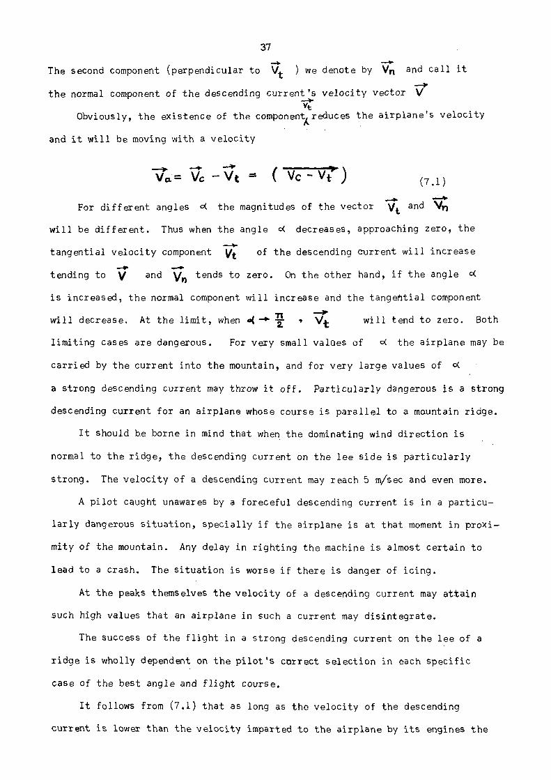
37

The second component (perpendicular to ) we denote by and call it

the normal component of the descending current's velocity vector

Obviously, the existence of the component reduces the airplane's velocity

and it will be moving with a velocity

For different angles α the magnitudes of the vector and

will be different. Thus when the angle α decreases, approaching zero, the

tangential velocity component of the descending current will increase

tending to and tends to zero. On the other hand, if the angle α

is increased, the normal component will increase and the tangential component

will decrease. At the limit, when will tend to zero. Both

limiting cases are dangerous. For very small values of α the airplane may be

carried by the current into the mountain, and for very large values of α

a strong descending current may throw it off. Particularly dangerous is a strong

descending current for an airplane whose course is parallel to a mountain ridge.

It should be borne in mind that when the dominating wind direction is

normal to the ridge, the descending current on the lee side is particularly

strong. The velocity of a descending current may reach 5 m/sec and even more.

A pilot caught unawares by a foreceful descending current is in a particu­

larly dangerous situation, specially if the airplane is at that moment in proxi­

mity of the mountain. Any delay in righting the machine is almost certain to

lead to a crash. The situation is worse if there is danger of icing.

At the peaks themselves the velocity of a descending current may attain

such high values that an airplane in such a current may disintegrate.

The success of the flight in a strong descending current on the lee of a

ridge is wholly dependent on the pilot's correct selection in each specific

case of the best angle and flight course.

It follows from (7.1) that as long as the velocity of the descending

current is lower than the velocity imparted to the airplane by its engines the

38

airplane wil l move in the same di rec t ion, but with a lower veloci ty than

However, the a i rc ra f t veloci ty in a very strong descending current may be

insuff ic ient to overcome the velocity of the descending current i . e . i t may be

that This i s one of the three dangerous cases in which the

a i rc ra f t i s bound to meet with accident and even catastrophe.

7 .3 .3 The level of maximum amplitude

After having determined whether waves of important amplitude are l ike ly

to occur, an attempt should be made to provide the p i lo t with information con­

cerning the level at which the waves wil l have the maximum amplitude. Such

information would enable the p i lo t to decide whether to climb or descend,

should be encounter troublesome waves. When the level of the maximum ampli­

tude i s near the level of mountain top, a knowledge of t h i s would be useful

in deciding on a safe f l ight l eve l .

Theory indicates tha t the level of maximum amplitude must be near the

level of maximum 12 . Since, when waves occur, t h i s parameter has a marked

maximum through some low or middle layer, the forecaster can safely predict

that the level of maximum amplitude will be somewhere in th i s layer, which

in general coincides with the layer of greates t s t a b i l i t y . The more pronoun­

ced the s t a b i l i t y , the closer to t h i s layer does the maximum amplitude of

waves tend to occur. In the case of a pronounced inversion, the forecaster

may confidently advise the p i lo t tha t the waves will be strongest at the

inversion level and tha t they wil l decrease rapidly above that l eve l .

Sometimes more than one wave system may prevail simultaneously at d i f f e -

rent l eve l s . This happens when the ve r t i ca l p rof i le of 12 shows more than

one maximum. The wave system associated with the different maxima wil l be

different because of the differences in wind speed at the i r respect ive

l e v e l s . In general , the upper wave system wil l have the longer wave-length.

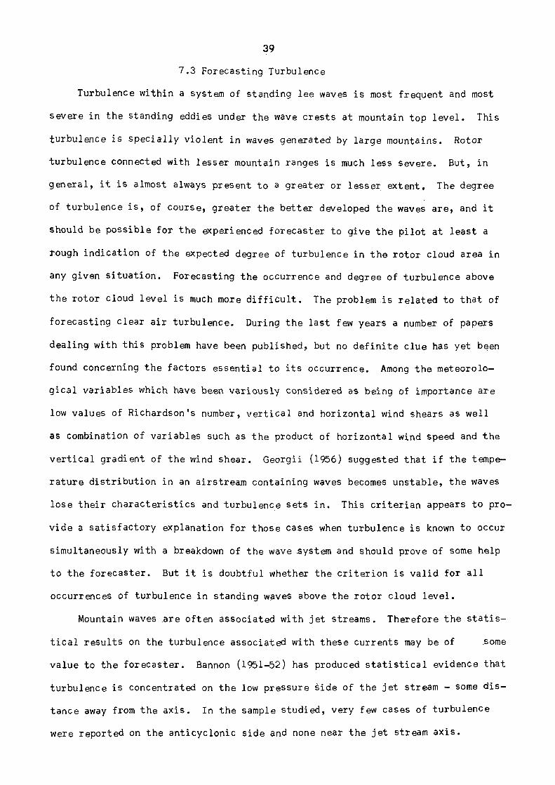
39

7.3 Forecasting Turbulence

Turbulence within a system of standing lee waves is most frequent and most

severe in the standing eddies under the wave crests at mountain top level. This

turbulence is specially violent in waves generated by large mountains. Rotor

turbulence connected with lesser mountain ranges is much less severe. But, in

general, it is almost always present to a greater or lesser extent. The degree

of turbulence is, of course, greater the better developed the waves are, and it

should be possible for the experienced forecaster to give the pilot at least a

tough indication of the expected degree of turbulence in the rotor cloud area in

any given situation. Forecasting the occurrence and degree of turbulence above

the rotor cloud level is much more difficult. The problem is related to that of

forecasting clear air turbulence. During the last few years a number of papers

dealing with this problem have been published, but no definite clue has yet been

found concerning the factors essential to its occurrence. Among the meteorolo­

gical variables which have been variously considered as being of importance are

low values of Richardson's number, vertical and horizontal wind shears as well

as combination of variables such as the product of horizontal wind speed and the

vertical gradient of the wind shear. Georgii (1956) suggested that if the tempe­

rature distribution in an airstream containing waves becomes unstable, the waves

lose their characteristics and turbulence sets in. This criterian appears to pro­

vide a satisfactory explanation for those cases when turbulence is known to occur

simultaneously with a breakdown of the wave system and should prove of some help

to the forecaster. But it is doubtful whether the criterion is valid for all

occurrences of turbulence in standing waves above the rotor cloud level.

Mountain waves are often associated with jet streams. Therefore the statis­

tical results on the turbulence associated with these currents may be of some

value to the forecaster. Bannon (1951-52) has produced statistical evidence that

turbulence is concentrated on the low pressure side of the jet stream - some dis­

tance away from the axis. In the sample studied, very few cases of turbulence

were reported on the anticyclonic side and none near the jet stream axis.

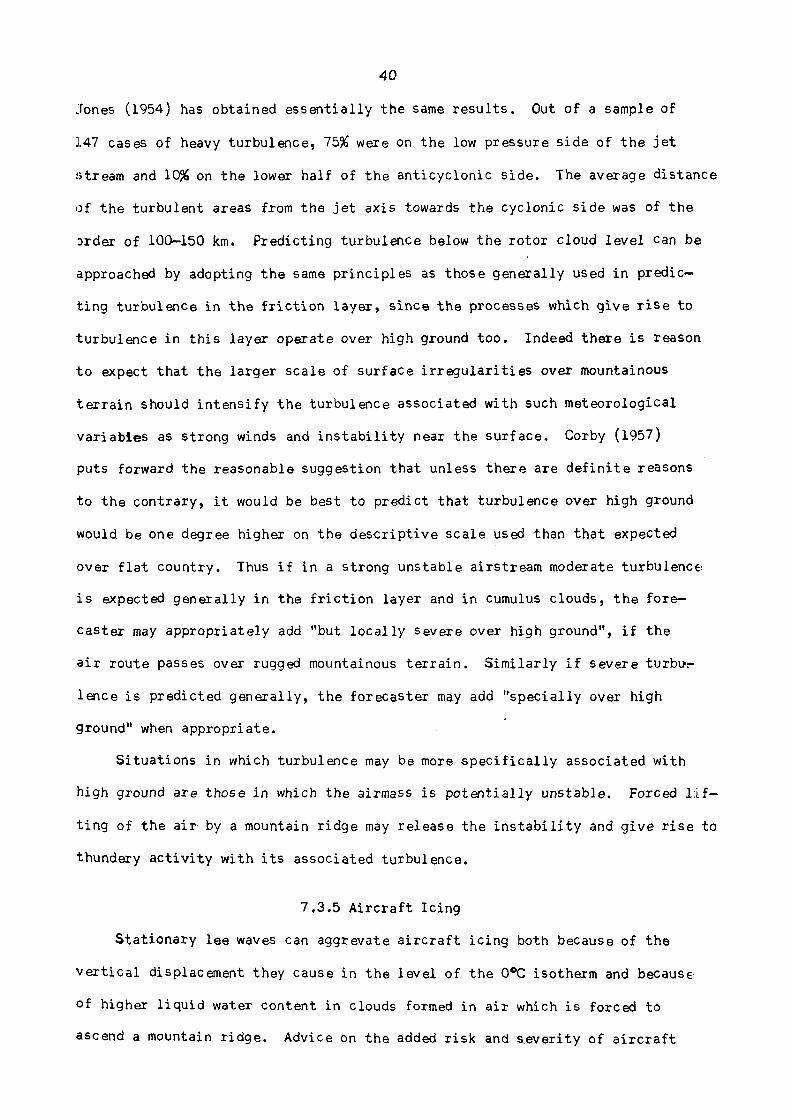
40

Jones (1954) has obtained essentially the same results. Out of a sample of

147 cases of heavy turbulence, 75% were on the low pressure side of the jet

stream and 10% on the lower half of the anticyclonic side. The average distance

of the turbulent areas from the jet axis towards the cyclonic side was of the

order of 100-150 km. Predicting turbulence below the rotor cloud level can be

approached by adopting the same principles as those generally used in predic­

ting turbulence in the friction layer, since the processes which give rise to

turbulence in this layer operate over high ground too. Indeed there is reason

to expect that the larger scale of surface irregularities over mountainous

terrain should intensify the turbulence associated with such meteorological

variables as strong winds and instability near the surface. Corby (1957)

puts forward the reasonable suggestion that unless there are definite reasons

to the contrary, it would be best to predict that turbulence over high ground

would be one degree higher on the descriptive scale used than that expected

over flat country. Thus if in a strong unstable airstream moderate turbulence

is expected generally in the friction layer and in cumulus clouds, the fore­

caster may appropriately add "but locally severe over high ground", if the

air route passes over rugged mountainous terrain. Similarly if severe turbu-

lence is predicted generally, the forecaster may add "specially over high

ground" when appropriate.

Situations in which turbulence may be more specifically associated with

high ground are those in which the airmass is potentially unstable. Forced lif­

ting of the air by a mountain ridge may release the instability and give rise to

thundery activity with its associated turbulence.

7.3.5 Aircraft Icing

Stationary lee waves can aggrevate aircraft icing both because of the

vertical displacement they cause in the level of the 0ºC isotherm and because

of higher liquid water content in clouds formed in air which is forced to

ascend a mountain ridge. Advice on the added risk and severity of aircraft

41

icing resulting from the above two factors would be very useful in aviation

forecasting.

Once the pattern of vertical motion is known, it is a straight-forward matter

to assess its effect on the level of the 0º isotherm from a representative soun­

ding in an undisturbed current. Since however the vertical motion in the mountain

waves varies with height in a manner which cannot be determined in a routine way,

some realistic assumption with regard to this motion must be made. A reasonable

basis for the present purpose is to assume that the air at all levels follows the

shape of the ground. Thus for an airstream crossing a mountain 1000 metres high

and containing stationary waves, it is assumed that the air is lifted at all

levels 1000 metres above its undisturbed level. The effect on the level of 0ºC

isotherm may then be determined from a tephigram by assuming dry adiabatic cooling

until saturation and wet adiabatic cooling above the condensation level. Some­

times it Seems likely that when a suitable airstream flows perpendicularly across a

long ridge, the amplitude of the wave may exceed that of the ground by a factor of

perhaps However if the height of the highest ground including that of the

individual peaks is used in applying the procedure some additional tolerance will

automatically be included. A suitable phrase for use in a forecast for a flight

over Assam and adjacent states in the winter might be "level of 0ºC isotherm

12000 ft (3.7 km) lowering to 10500 ft (3.2 km) over the hills". In general, if

the levels at which icing is expected coincide with a layer in which waves are

likely to exist, the forecaster should predict worse icing conditions than he

would otherwise.

Apart from the possible lowering of the level of the 0ºC isotherm, the effect

of mountain on the intensity of icing due to increased liquid water content need

also be considered. Icing is a complicated matter involving both meteorological

and aerodynamic quantities. The most important of the meteorological variables

is the concentration of supercooled liquid water in the potential icing cloud.

This is a difficult quantity to be measured. But such measurements as have

been made from aircraft have rarely values greater than 1 gm/m3, whereas at

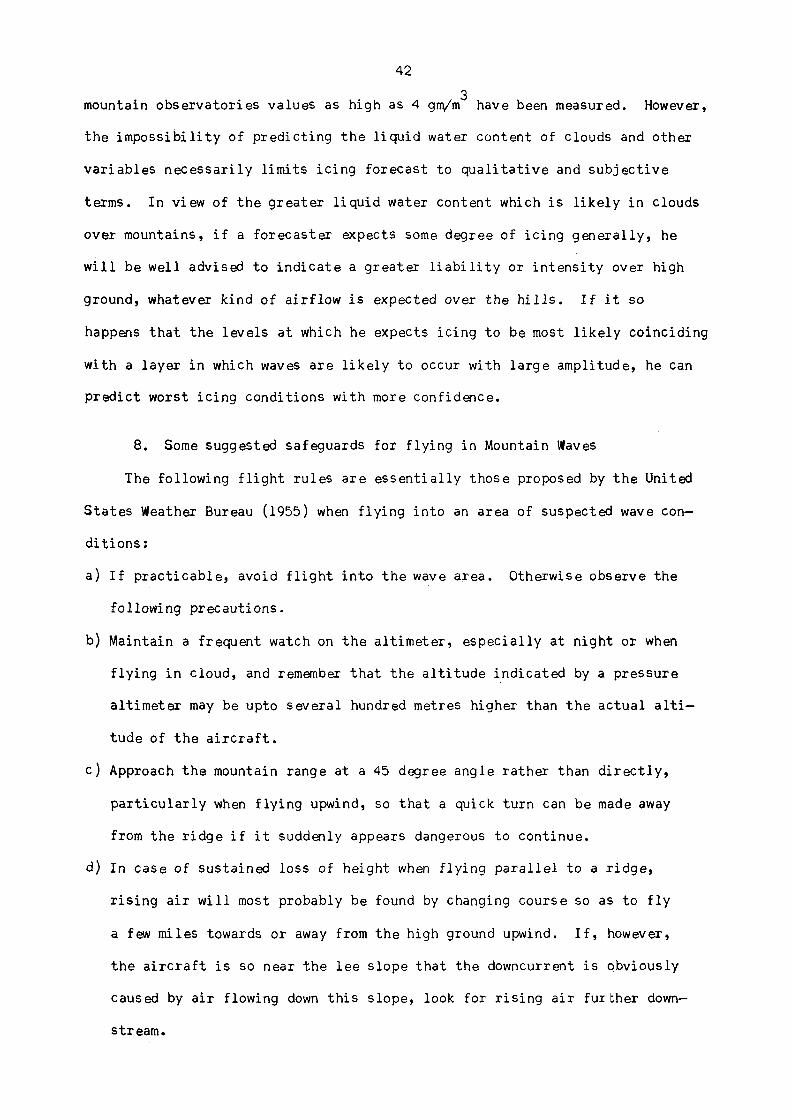
42

mountain observatories values as high as 4 gm/m3 have been measured. However,

the impossibility of predicting the liquid water content of clouds and other

variables necessarily limits icing forecast to qualitative and subjective

terms. In view of the greater liquid water content which is likely in clouds

over mountains, if a forecaster expects some degree of icing generally, he

will be well advised to indicate a greater liability or intensity over high

ground, whatever kind of airflow is expected over the hills. If it so

happens that the levels at which he expects icing to be most likely coinciding

with a layer in which waves are likely to occur with large amplitude, he can

predict worst icing conditions with more confidence.

8. Some suggested safeguards for flying in Mountain Waves

The following flight rules are essentially those proposed by the United

States Weather Bureau (1955) when flying into an area of suspected wave con­

ditions:

a) If practicable, avoid flight into the wave area. Otherwise observe the

following precautions.

b) Maintain a frequent watch on the altimeter, especially at night or when

flying in cloud, and remember that the altitude indicated by a pressure

altimeter may be upto several hundred metres higher than the actual alti­

tude of the aircraft.

c) Approach the mountain range at a 45 degree angle rather than directly,

particularly when flying upwind, so that a quick turn can be made away

from the ridge if it suddenly appears dangerous to continue.

d) In case of sustained loss of height when flying parallel to a ridge,

rising air will most probably be found by changing course so as to fly

a few miles towards or away from the high ground upwind. If, however,

the aircraft is so near the lee slope that the downcurrent is obviously

caused by air flowing down this slope, look for rising air further down­

stream.

43

e) It is possible when flying into the wind to utilise updraft areas to gain

height. In particular look for rising currents upwind of the rotor cloud and

also of the lenticular clouds if they happen to be near flight level. Caution

should, however, be exercised in employing this procedure, since it is not

always possible to pinpoint the updraft areas.

f) Avoid flying into the rotor clouds. Also avoid the lenticular clouds when

their edges are torn and irregular.

g) Avoid flying through a powerful wave on instruments

h) Because of strong downdrafts and turbulence, and the hazards of instrument

flight near mountain tops, avoid flying into a cap cloud, even if it means

turning back.

9. Mountain waves over Western Ghats

Sarker (1965, 67) studied the occurrence of mountain waves on the lee of the

Western Ghats theoretically. The average W-E vertical cross section of the ghats

near the Bombay-Poona region (Fig. 10) was represented by

where the elevation of the ground surface at the level z = -h with the

numerical values h = 0.25 km, a = 1.8 km, b = 0.52 km and km.

Expressions for vertical velocity and streamline displacement due to waves were

established for a two—dimensional motion. Computation for six cases has been made

for the winter season when the wind is more or less westerly and the atmosphere is

dry (Sarker 1965). The wind and temperature profiles for two of these cases are

shown in Figs. 11(a) - 12(a) and the corresponding f(z) profiles are shown in

Figs. 11(b) - 12(b). It will be seen from the f(z) profiles at once that lee waves

are possible in all these cases. The wavelengths and maximum vertical velocity

associated with the waves are shown in Table 4. The variation of maximum ampli­

tude and maximum vertical velocity for these cases are shown in Figs. 13(a), 13(b),

14(a), 14(b). The streamline displacement for one case is shown in Fig. 15.

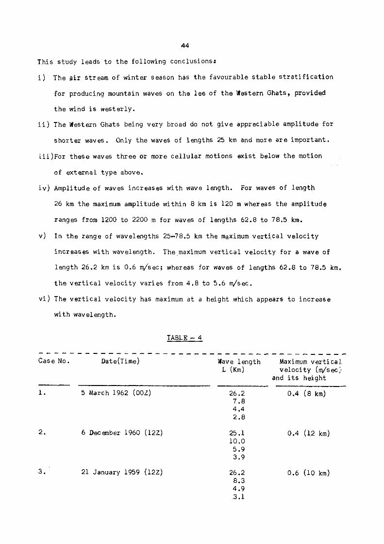
44

This s tudy leads to t h e following conclus ions :

i ) The a i r s tream of winter season has t h e favourable s t a b l e s t r a t i f i c a t i o n

for producing mountain waves on t h e l e e of t h e Wes te rn Gha t s , provided

t h e wind i s w e s t e r l y ,

i i ) The Western Ghats being very broad do not g ive apprec i ab le ampl i tude for

s h o r t e r waves. Only t h e waves of lengths 25 km and more a r e impor t an t .

i i i ) For t h e s e waves t h r e e or more c e l l u l a r motions ex i s t below t h e motion

of e x t e r n a l type above.

i v ) Amplitude of waves i n c r e a s e s wi th wave l e n g t h . For waves of l eng th

26 km t h e maximum ampli tude wi th in 8 km i s 120 m whereas t h e ampl i tude

ranges from 1200 to 2200 m for waves of l eng ths 62 .8 to 78.5 km.

v) In t h e range of wavelengths 25-78.5 km t h e maximum v e r t i c a l v e l o c i t y

i n c r e a s e s wi th wavelength. The maximum v e r t i c a l v e l o c i t y for a wave of

length 26.2 km i s 0.6 m / s e c ; whereas for waves of l eng ths 62 ,8 t o 78.5 km.

t h e v e r t i c a l v e l o c i t y v a r i e s from 4 . 8 to 5 .6 m/sec .

v i ) The v e r t i c a l v e l o c i t y has maximum at a height which appears t o i n c r e a s e

with wavelength.

Case No. Date(Time) Wave l eng thL (Km)

Maximum v e r t i c a l

v e l o c i t y (m/sec)

and i t s he ight

1 . 5 March 1962 (00Z) 26.27 . 84 . 42 . 8

0.4 (8 km)

2 . 6 December 1960 (12Z) 25 .110.0

5 .93.9

0.4 (1,2 km)

3 . 21 January 1959 (12Z) 26.2

8.3

4 . 9

.3.1

0.6 (10 km)

TABLE - 4

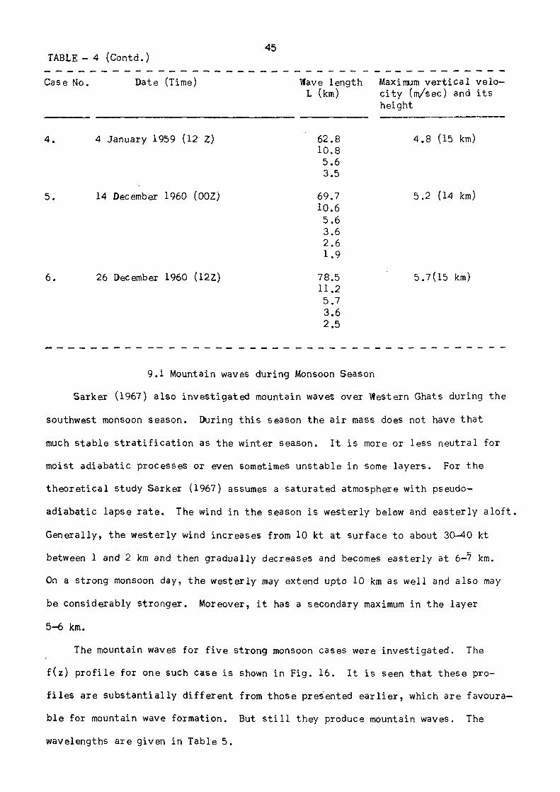
45

TABLE - 4 (Contd.)

Case No. Date (Time) Have length

L (km)

Maximum vertical velo­

city (m/sec) and its

height

4. 4 January 1959 (12 2) 62,8

10.8

5.6

3.5

4.8 (15 km)

5. 14 December 1960 (00Z) 69.7

10.6

5.6

3.6

2.6

1.9

5.2 (14 km)

6. 26 December 1960 (12Z) 78.5

11.2

5.7

3.6

2.5

5.7(15 km)

9.1 Mountain waves during Monsoon Season

Sarker (1967) also investigated mountain waves over Western Ghats during the

southwest monsoon season. During this season the air mass does not have that

much stable stratification as the winter season. It is more or less neutral for

moist adiabatic processes or even sometimes unstable in some layers. For the

theoretical study Sarker (1967) assumes a saturated atmosphere with pseudo-

adiabatic lapse rate. The wind in the season is westerly below and easterly aloft.

Generally, the westerly wind increases from 10 kt at surface to about 30-40 kt

between 1 and 2 km and then gradually decreases and becomes easterly at 6-7 km.

On a strong monsoon day, the westerly may extend upto 10 km as well and also may

be considerably stronger. Moreover, it has a secondary maximum in the layer

5-6 km.

The mountain waves for five strong monsoon cases were investigated. The

f(z) profile for one such case is shown in Fig. 16. It is seen that these pro­

files are substantially different from those presented earlier, which are favoura­

ble for mountain wave formation. But still they produce mountain waves. The

wavelengths are given in Table 5.

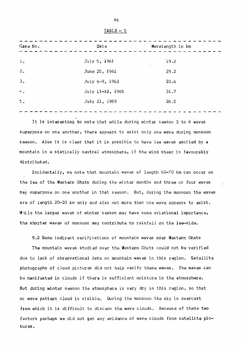
46

TABLE - 5

Case No. Date Wavelength in km

1. July 5, 1961 19.2

2. June 25, 1961 29.2

3. July 6-9, 1963 20.6

4. July 11-12, 1965 31.7

5. July 21, 1959 26.5

I t i s in te res t ing to note that while during winter season 3 to 4 waves

superpose on one another, there appears to exist only one wave during monsoon

season. Also i t i s clear that i t i s possible to have lee waves excited by a

mountain in a s t a t i c a l l y neutral atmosphere, if the wind shear i s favourably

d i s t r ibu ted .

Inc identa l ly , we note that mountain waves of length 60-70 km can occur on

the lee of the Western Ghats during the winter months and three or four waves

may superpose on one another in that season. But, during the monsoon the waves

are of length 20-30 km only and also not more than one wave appears to ex is t .

While the larger waves of winter season may have some aviat ional importance,

the shorter waves of monsoon may contr ibute to r a in f a l l on the l ee - s ide .

9.2 Some indirect ver i f ica t ions of mountain waves over Western Ghats

The mountain waves studied over the Western Ghats could not be ver i f ied

due to lack of observational data on mountain waves in th is region. S a t e l l i t e

photographs of cloud pictures did not help verify these waves. The waves can

be manifested in clouds if there i s suff icient moisture in the atmosphere.

But during winter season the atmosphere i s very dry in th i s region, so that

nc wave pattern cloud i s v i s i b l e . During the monsoon the sky i s overcast

from which i t i s d i f f i cu l t to discern the wave clouds. Because of these two

factors perhaps we did not get any evidence of wave clouds from s a t e l l i t e p i c ­

t u r e s .

47

However, perhaps some indirect evidence can be had from the following:

9.2.1 Leewaves from cloud observations

Sinha (1966) observed on 6 March 1965 orographic clouds at Matheran

(Lat. 18º 58'N, Long. 73º 18'E) which is a hill station situated at the Western

Ghats on the top of a narrow long and rather isolated north-south steep ridge.

The ridge is about 750 m high, about 2 km wide and 9 km long at the top. It is

situated about 50 km to the east of Bombay. Two rows of clouds were estimated

to be at a height of 1500 m. Their thickness was estimated to be 200 m approxi­

mately. The wavelength inferred from the estimated vertical angle and the height

of the clouds was between 1 to 2 km.

Our theoretical computation for this case was made by fitting the profile

with numerical values a = 0.5 km, b = 0.75 km for Matheran.

The f(z) profile for this is given in Fig. 17. Fitting a two layer model for

f(z) profile, the theoretical computation shows that wavelength L = 2.7 km. The

wave amplitudes are 426 m, 206 m and 70 m. at heights 1 km, 1.5 km and 2 km

respectively. The maximum vertical velocities at these levels are 3.2 m/sec.

1.9 m/sec and 0.7 m/sec. These theoretical values of wavelength and wave ampli­

tude at 1.5 km agree fairly well with the estimated values of wavelength and

cloud thickness at 1.5 km.

9.2.2 Turbulence Reports by Aircraft

i) On 9 December 1964 a Boeing 707 in its flight from Madras to Bombay

reported light continuous clear air turbulence at 1759 IST when its position was

15º 40'N, 76º 10'E, well on the lee of the Western Ghats, at a height of

28500 ft (roughly 9 km). The duration of this turbulence was reported to be

6 minutes. The speed of the aircraft was approximately 700 miles/hour, so that

in 6 minutes it goes about 70 miles, i.e. 110 kms. That is, during this period

the aircraft was on the lee of the Western Ghats.

Our theoretical investigation shows that there were mountain waves both in

the morning and in the evening on that day. The wave length for morning was

48

31 km and for evening 19.4 km. Corresponding to the wavelength of 19.4 km the

maximum ver t i ca l velocity at 9 km was about 10 cm/sec. The a i rc raf t would have

crossed five wavelengths during i t s f l ight on the lee s ide and would have

f e l t the up and down undulations about ten times. This might be the reason for

the continuous l ight turbulence, although i t i s not possible to say if turbu-

lence might be due to other causes.

i i ) On 11 December 1964 a Comet 4 in i t s f l ight from Colombo to Karachi repor­

ted l ight continuous clear a i r turbulence at 1335 IST at a height of 32000 ft

(roughly 10 km) while i t s position was 14ºN, 75ºE, on the lee side of the

Western Ghats. The duration of turbulence was 2 minutes. The speed of the

a i r c ra f t was roughly 500 miles/hr so that in two minutes i t crossed 17 miles,

i . e . 30 kms approximately. That i s in 2 minutes i t has come to the windward

s ide , outside the lee wave, if any.

Our theore t ica l computation shows that on t h i s day there were mountain

waves both in the morning and the evening. The wavelength for the morning

works out to be 18 km and for the evening i t i s 44 km. The corresponding

maximum ver t i ca l veloci ty at 10 km works out to be 10 cm/sec and 190 cm./sec

respect ive ly . I t . i s quite possible that the turbulence reported by the a i r ­

craf t might be in association with the waves, although there i s no direct way

of ve r i f i ca t ion .

10. Mountain waves over Assam-Burma Hills

De (1970) invest igated the presence of mountain waves over the Assam

and Burma Hil ls with the help of s a t e l l i t e p ic tu res . He studied in a l l six-

teen cases for which the wavelengths as observed from the s a t e l l i t e photo­

graphs vary between 17-34 km. The observed wavelengths have also been com­

pared with the wavelengths computed theo re t i ca l ly . Some of these cases are

presented in Table 6.

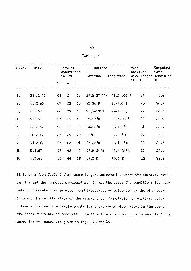
49

TABLE - 6

S.No. Date Time ofoccurrencein GMT

Location Meanobservedwave lengthin km

Computed

wave­

leng th in

km

S.No. Date Time ofoccurrencein GMT L a t i t u d e Longitude

Meanobservedwave lengthin km

Computed

wave­

leng th in

km

S.No. Date

h m s

L a t i t u d e Longitude

Meanobservedwave lengthin km

Computed

wave­

leng th in

km

1 . 23.11.66 08 0 22 26 .5-27 .5 ºN 98.5-100ºE 23 19.6

2 . 1.12.66 07 02 00 25-26 °N 99-100°E 20 20 .9

3 . 8.1.67 06 29 15 27.5-29ºN 99-101°E 22 2 6 . 3

4 . 9 .1 .67 07 19 40 25-27 °N 99.5-102°E 22 22.0

5 . 13.2 .67 06 11 30 24-26 °N 98-101°E 31 26.1

6 . 10 .2 .67 07 29 29 25 °N 94-95°E 17 17.1

7 . 14.2 .67 07 02 01 25-26ºN 98-100ºE 22 23 .6

8. 5 .3 .67 07 43 43 23.5-24ºN 93.5-95°E 21 20 .1

9 . 9 .2 .68 05 44 38 27.5°N 99.5°E 23 22.2

It is seen from Table 6 that there is good agreement between the observed wave­

lengths and the computed wavelengths. In all the cases the conditions for for­

mation of mountain waves were found favourable as evidenced by the wind pro­

file and thermal stability of the atmosphere. Computation of vertical velo­

cities and streamline displacements for these cases given above in the lee of

the Assam hills are in progress. The satellite cloud photographs depicting the

waves for two cases are given in Figs. 18 and 19.

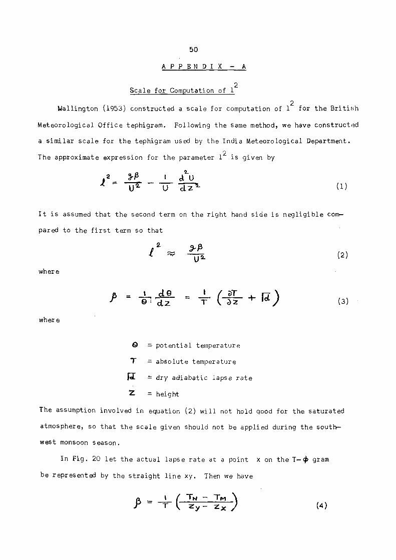
50

A P P E N D I X - A

Scale for Computation of 12

Wallington (1953) constructed a scale for computation of 12 for the Br i t i sh

Meteorological Office tephigram. Following the same method, we have constructed

a similar scale for the tephigram used by the India Meteorological Department.

The approximate expression for the parameter 12 i s given by

I t i s assumed that the second term on the r ight hand side i s negl igible com­

pared to the f i r s t term so that

where

where

θ = potential temperature

τ = absolute temperature

= dry adiabatic lapse rate

Z = height

The assumption involved in equation (2) will not hold good for the saturated

atmosphere, so that the scale given should not be applied during the south-

west monsoon season.

In Fig. 20 let the actual lapse rate at a point x on the T-Φ gram

be represented by the straight line xy. Then we have

51

where the subscripts refer to the points considered. From Fig.20 we get

Zy - Zx = ZL - ZX, the latter quantity representing a height interval along an

isotherm.

By integrating the hydrostatic equation along this interval we get

where p, R, g, A and denote respectively the pressure, the appropriate gas

constant, the acceleration due to gravity, the reciprocal of the mechanical

equivalent of heat and the entropy. (A appears if the work done by gas is

expressed in thermal units).

From equations (4) and (5) we have

and

TN-TM and are measured by the lengths NM and LX respectively.

Therefore,

where K is a constant appropriate to the scale of the diagram. Assuming the

angle XMY constant and equal to 45º, we have

He now construct a triangle XPQ similar to XMY such that PX is proportional to

T—2 . This leads to

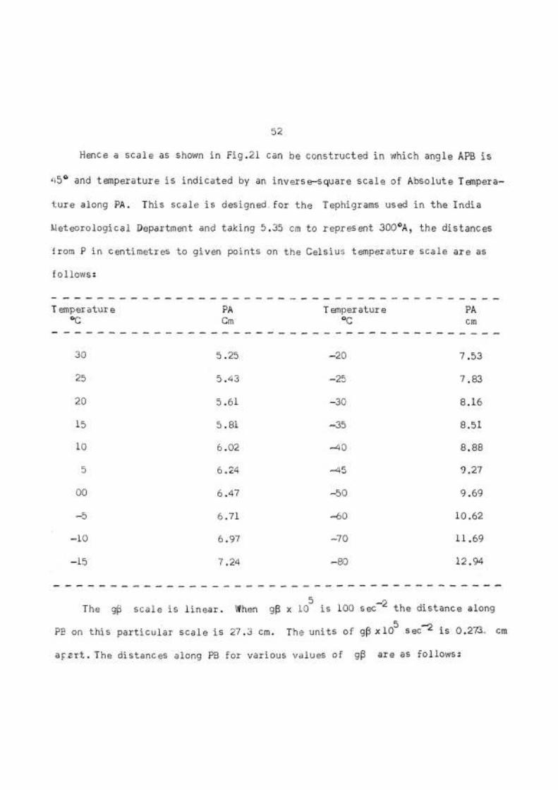
52

Hence a scale as shown in Fig.21 can be constructed in which angle APB i s

45º and temperature i s indicated by an inverse-square scale of Absolute Tempera-

ture along PA. This scale i s designed, for the Tephigrams used in the India

Meteorological Department and taking 5.35 cm to represent 300ºA, the distances

from P in centimetres to given points on the Celsius temperature scale are as

follows:

Temperature°C

PA

Cm

Temperature°C

PA

cm

30 5.25 -20 7.53

25 5.43 -25 7.83

20 5.61 -30 8.16

15 5.81 -35 8.51

10 6.02 -40 8.88

5 6.24 -45 9.27

00 6.47 -50 9.69

- 5 6.71 -60 10.62

-10 6.97 -70 11.69

-15 7.24 -80 12.94

The gβ scale is l i nea r . When gβ × 105 i s 100 sec-2 the distance along

PE on th is par t icular scale i s 27.3 cm. The units of gβ × 105 sec-2 i s 0.273 cm

a p a r t . The distances along PB for various values of gβ are as follows:

53

gβ × 105 s e c

- 2PB cm gβ × 10

5 sec

- 2 PB

4 1.09 44 12.03

8 2.19 48 13.13

12 3.28 52 14.22

16 4 .38 56 15.32

20 5.47 60 16.41

24 6.56 64 17.50

28 7.66 68 18.60

32 8.75 72 19.69

36 9.85 76 20.79

40 10.94 80 21.88

Scales for other forms and units can be constructed by applying the

appropriate conversion factors.

Using the Scale

For convenient computation of 12, the above scale is constructed on a

Celluloid. To find the values of gβ at a particular level, say X of a given

curve, the scale is laid on the tephigram so that PA is parallel to

the dry adiabatic with the appropriate temperature at X. The lapse rate in the

vicinity of X is produced to intersect PB where the required value of

gβ × 105 sec-2 can be read off directly. The method is illustrated in Fig. 21.

Division by U2 then yields the approximate value of 12.

In practice it is generally sufficient to evaluate the mean value of 12

for 50 mb layers. In doing so, the following should be noted:

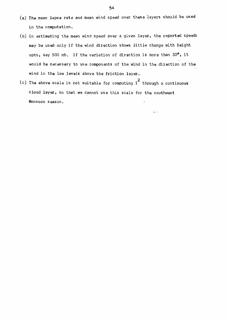
54

(a) The mean lapse rate and mean wind speed over these layers should be used

in the computation.

(b) In estimating the mean wind speed over a given layer, the reported speeds

may be used only if the wind direction shows little change with height

upto, say 500 mb. If the variation of direction is more than 30º, it

would be necessary to use components of the wind in the direction of the

wind in the low levels above the friction layer.

(c) The above scale is not suitable for computing 12 through a continuous

cloud layer, so that we cannot use this scale for the southwest

Monsoon season.

55

A P P E N D I X - B

Graphical Determination of Wavelength

In Appendix A we have given a scale to compute 12 from a tephigram

directly. In this appendix we shall show how to calculate wave length graphi-

cally from the distribution of 12.

I t was shown in section 6.3 that when 12 can be represented by an exponen­

t i a l function of the form

the wavelength i s given by

m being the roots of

For a s t a t i c a l l y s tab le atmosphere 12 can be generally represented by equation

(1) so that we can wri te

and then wave number i s given by

The walues of 1(z) obtained by the method given in Appendix A are then plot ted

in a simple logarithmic graph paper as given in Fig.22.

The exponential decrease of 1 i s represented by a s t ra igh t l ine due to the

logarithmic scale used. This l ine determines the parameters 1(0) and C. The

intersec t ion of the l ine with the horizontal log scale gives 1(0) . The

parameter C is derived by the formula

where i s the angle of inc l in ina t ion of the s t r a igh t l ine with the

ver t i ca l and P is a constant dependent on the scale of the diagram. In our

case the value of P i s 0.7675 km-1

. I t can be calculated easily for any

other sca le .

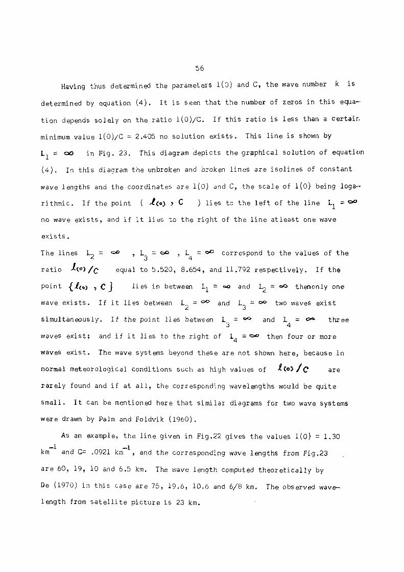
56

Having thus determined t h e parameters 1(0) and C, t h e wave number k i s

determined by equation ( 4 ) , I t i s seen t h a t t h e number of zeros in t h i s equa­

t i o n depends s o l e l y on t h e r a t i o 1 ( 0 ) / C . If t h i s r a t i o i s l e s s than a c e r t a i n

minimum va lue 1 (0 ) /C = 2.405 no s o l u t i o n e x i s t s . This l i n e i s shown by

L1 = ∞ in F ig . 2 3 . This diagram dep ic t s t h e g r aph i ca l s o l u t i o n of equation

( 4 ) . In t h i s diagram t h e unbroken and broken l i n e s are i s o l i n e s of cons tan t

wave leng ths and t h e coord ina tes a r e 1(0) and C, t h e s c a l e of 1(0) being l o g a ­

r i t h m i c . If t h e point ( (o), C ) l i e s to t h e l e f t of t h e l i n e L1 = ∞

no wave e x i s t s , and i f i t l i e s to t h e r i g h t of t h e l i n e a t l e a s t one wave

e x i s t s .

The l i n e s L2 = ∞, L3 = ∞, L4 = ∞ correspond to t h e va lues of t h e

r a t i o equal to 5 .520, 8.654, and 11.792 r e s p e c t i v e l y . I f t h e

po in t { (o), C} l i e s in between L1 = ∞ and L2 = ∞ then only one

wave e x i s t s . I f i t l i e s between L2 = ∞ and L3 = ∞ two waves e x i s t

s imu l t aneous ly . I f t h e point l i e s between L3 = ∞ and L4 = ∞ t h r e e

waves e x i s t ; and i f i t l i e s to t h e r i g h t of L4 = ∞ then four or more

waves e x i s t . The wave systems beyond t h e s e a re not shown he re , because in

normal meteoro logica l cond i t ions such as high values of a re

r a r e l y found and i f at a l l , t h e corresponding wavelengths would be q u i t e

Smal l . I t can be mentioned here t h a t s i m i l a r diagrams for two wave systems

were drawn by Palm and Foldvik (1960) .

As an example, t h e l i n e given in Fig.22 g ives t h e values 1(0) = 1.30

km-1 and C= .0921 km-1 , and t h e corresponding wave lengths from F ig .23

a r e 60, 19, 10 and 6.5 km. The wave length computed t h e o r e t i c a l l y by

De (1970) in t h i s case a r e 75 , 1 9 . 6 , 10.6 and 6/8 km. The observed wave­

l eng th from s a t e l l i t e p i c t u r e i s 23 km.

57

REFERENCES

1. Alaka, M.A. 1958: Aviation Aspects of Mountain waves, WMO Tech. Note 18,

p. 47.

2 . Bannon, J .K. 1951: Meteorological Aspects of Turbulence Affect ing A i r c r a f ta t High A l t i t u d e s - Prof. Notes 7 , No.104.

3 . Bannon, J .K . 1952: Weather systems Associated with some occasions of

seve re Turbulence a t High A l t i t u d e , Met. Mag. V o l . 8 1 .

4 . Berenger , M. e t . Gerb ie r , N. 1956: Monographie No.4, de 1a Meteorologie

N a t i o n a l e . Roy. Met. Soc. 87, pp .13 -23 .

5. Cohen, A. Doron, E. 1966: Meteorological satellite data of report of

studies. Report of work performed under contract C.W.B. 11055.

6. Colson, De Ver. 1954: Results of double theodolite observations at B1 shop,

Cal., in connection with the "Bishop wave" phenomenon. Bull.Amer.

Met. Soci. 33, pp.107-146.

7. Corby, G.A. 1957: Airflow over mountains: Notes for forecasters and pilots.

Met.Rep.No.18, H.M. Stationery office.

8. Corby G.A. 1957: A preliminary study of atmospheric waves using radiosonde

data. Quart. J.R. Met. Soc. Vol.83, pp.49-60.

9. Corby, G.A. and Wallington, C.E. 1956: Airflow over mountains: the lee-

wave amplitude Q.J.R.M.S. 82, pp.266-274.

10. De, U.S. 1970: Lee wavesas evidenced by satellite cloud pictures. IJMG

Vol.21, No.4, pp.637-642.

11. Doos, BO.R. 1961: Tellus, Vol.13, No.3, pp.305-319.

12. Doos, Bo. R. 1962: Tellus Vol.14, No.3, pp.301-309.

13. Foldvik, A. 1962: QJRMS Vol.88, pp.271-285.

14. Forchtgott, J. 1949: Wave streaming in the lee of mountain ridges Bull.

Met. Czech, Prague, 3, p.49.

15. Forchtgott, J. 1951: The air flow round a conical hill. Gliding, Vol.2,

p. 147.

16. F r i t z , S . 1965: The s i g n i f i c a n c e of mountain l ee waves as seen from s a t e l ­l i t e p i c t u r e s - J r . Appl. Met .Vol .4 , No .1 , pp .31-37 .

17. Gerb ie r , N. and Berenger, M. 1961: QJRMS, 87 pp .13 -23 .

18 . Kue t tner , J . 1939: B e i t r . Phys. F r e i . Atmos. 2 5 , pp.79-114.

19 . Kue t tne r , J . and J e n k i n s , C F . 1953: F l i g h t a spec t s of t h e mountain wave.

Air Force Cambridge Research Cen t re , Surveys in Geophysics, Tech.

Report No.35.

20 . Jones , D.C.E. 1954: Fur ther I n v e s t i g a t i o n s of High Level c l e a r Air Turbu­

l e n c e . Met. Mag. V o l . 8 3 .

58

2 1 . Larson, L. 1954: Observat ions of l e e wave clouds in t h e Jamtland Mountains,Sweden, T e l l u s , 6, pp.124-138.

22 . Ludlam, F.A. 1952: Orographic c i r r u s clouds QJRMS 78 , p .558 .

2 3 . Manley, G. 1945: The Helm wind of C r o s s f e l l , 1937-1939. QJRMS 7 1 , pp .197-

219.

24 . Mason, D. 1954: H i l l s s tanding waves and s a f e t y he igh t s , W e a t h e r , London.p . 4 5 .

2 5 . Musaelyan, Sh.A. 1960: B a r r i e r waves in t h e Atmosphere. T rans l a t ed fromRuss ian . I s r a e l Program for s c i e n t i f i c T r a n s l a t i o n s , Je rusa lem,1964.

2 6 . Palm, E. 1958: Geophy. Publ . Vol .20, No.3 , Os lo .

2 7 . Palm E. and Foldvik , A. 1960: Geo. Publ . Vo l .21 , No.6, Oslo , pp. 30.

2 8 . P i l s b u r y , R.R. 1955: A pre l iminary a n a l y s i s of s tanding wave r e p o r t srece ived a t Nor thhol t during t h e winter of 1953-1954. Met. Mag. 84,pp.313-318.

2 9 . Queney, P. 1947: Theory of p e r t u r b a t i o n s in s t r a t i f i e d c u r r e n t s wi tha p p l i c a t i o n to a i r f low over mountain b a r r i e r . The Unive r s i ty ofChicago P r e s s , Misc. Rep. No.23.

3 0 . Queney, P. 1948: The problem of a i r f low over mountains . A summary oft h e o r e t i c a l s t u d i e s — B u l l . Amer. Met. Soc . 29 , pp .16-26 .

3 1 . Queney, P. et a l . 1960: The a i r f low over mountains, WMO Tech. Note 34,

p . 135.

3 2 . S a r k e r , R.P. 1965: "A T h e o r e t i c a l s tudy of Mountain waves on Western

Ghats" IJ Met. and Geophy. Vol .16, No.4, pp.565-584.

3 3 . S a r k e r , R.P. 1967: "Some Modif icat ion in Dynamical Model of orographicr a i n f a l l " , Monthly Weather Review, U.S. Weather Bureau Vol .95 , No. 10, pp.673-684.

3 4 . Sawyer, J . S . 1960: QJRMS Vol .86 , pp.326-345.

3 5 . Sco re r , R.S. 1949: Theory of waves in t h e l e e of mountains . QJRMS 7 5 ,pp .41-56 .

36. Scorer, R.S. 1953: Theory of airflow over mountains, II: The flow

over a ridge. QJRMS 79, pp.70-83.

37. Scorer, R.S. 1954: Theory of airflow over mountains, III: Airflow

characteristics, QJRMS, 80, pp.417-428.

38. Scorer, R.S. 1955: Theory of airflow over mountains IV: Separation of

airflow from the surface, QJRMS, 81, pp.340-350.

39. Scorer, R.S. 1956: "Airflow over an isolated hill". QJRMS 82,

pp. 75-81.

59

4 0 . S c o r e r , R.S. and Wilkinson, M. 1956: "Waves in t h e l e e of an i s o l a t e dh i l l " . QJRMS 82, pp.419-427.

41. Sinha, M.C. 19662 "Mountain lee waves over western Ghats". IJMG Vol.17,

No. 3, pp.419-420.

4 2 . Stormen, C. 1948: "Mother of Pear l c louds" , Weather, London, 3 , p . 1 3 .

4 3 . Wal l ington , C.E. 1953: OPS-ENG Report , I n t e r n a t i o n a l Air Transpor t

Association.

DIAGRAMS

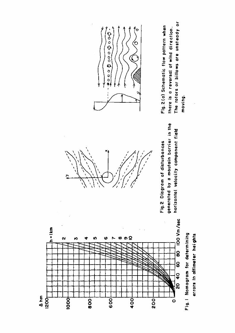
Fig

. I

No

mo

gra

m

for

de

term

inin

g

err

ors

in

a

ltim

ete

r h

eig

hts

Fig

. 2

Dia

gra

m

of

dis

turb

an

ce

s

ge

ne

rate

d

by

a

mo

uta

in

ba

rrie

r in

th

e

ho

rizo

nta

l v

elo

cit

y

co

mp

on

en

t fi

eld

Fig

. 2

(a)

Sc

he

ma

tic

flo

w

pa

tte

rn

wh

en

the

re

is

a re

ve

rsa

l o

f w

ind

d

ire

cti

on

.

Th

e

roto

rs

or

bil

low

s

are

u

ns

tea

dy

or

mo

vin

g.

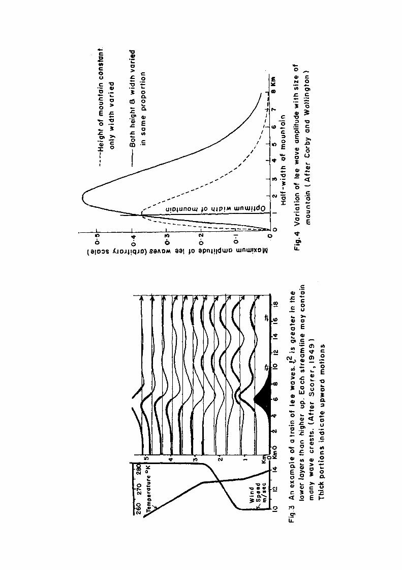
Fig

. 3

An

ex

am

ple

o

f a

tra

in o

f le

e

wa

ve

s2

is g

rea

ter

in th

e

low

er

layers

th

an

h

igh

er

up

. E

ac

h s

tre

am

lin

e

may c

on

tain

man

y

wa

ve

cre

sts

. (A

fte

r S

co

rer,

1

94

9)

Th

ick p

ort

ion

s

ind

ica

te

up

wa

rd

mo

tio

ns

Fig

. 4

Va

ria

tio

n of

lee w

ave am

plit

ud

e w

ith

siz

e

of

mo

un

tain

(A

fte

r C

orb

y

an

d

Wa

llin

gto

n)

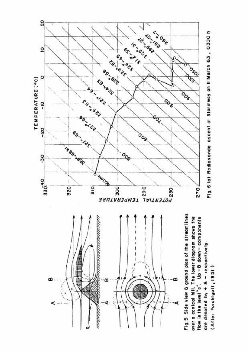
Fig

. 5

S

ide vie

w &

gro

un

d p

lan

of

the

str

ea

mli

ne

s

over

a c

on

ica

l h

ill.

Th

e lo

wer

dia

gra

m

sh

ow

s

the

flo

w

in t

he

lev

el "a

".

Up

- &

d

ow

n-

co

mp

on

en

ts

are

d

en

ote

d

by +

8

- re

sp

ec

tiv

ely

.

( A

fte

r F

orc

htg

ott

, 1

95

1)

Fig

. 6

(a

) R

ad

ios

on

de

as

ce

nt

at

Sto

rmw

ay

on

II

Ma

rch

6

3,

03

00

h

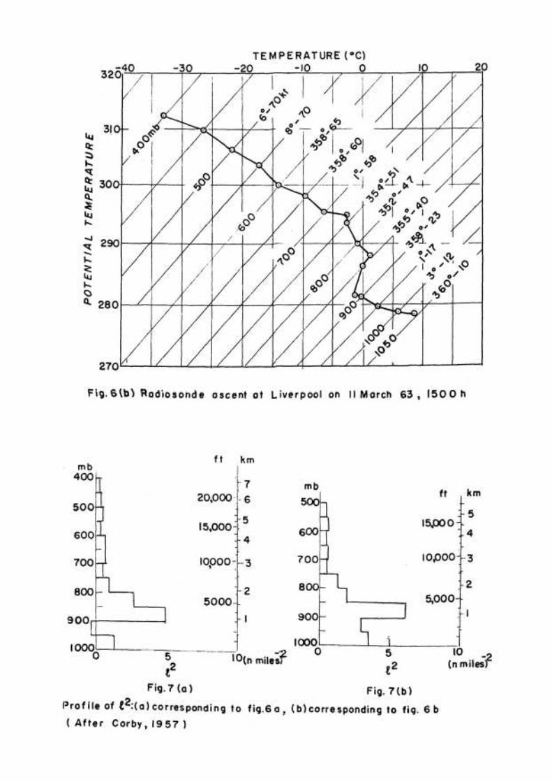
Fig. 6(b) Radiosonde ascent at Liverpool on II March 6 3 , 1500 h

Fig. 7 ( a ) Fig. 7(b)

Profile of 2:(a) corresponding to fig. 6a, (b) corresponding to fig. 6 b

( A f t e r Corby, 1 9 5 7 )

Fig

. 8

(b)

The

co

rre

sp

on

din

g p

rofile

of

2

(Aft

er

Co

rby

1957)

Fig

. 8

(a)

Ra

dio

so

nd

e

ob

se

rva

tio

n

at

Ald

erg

rov

e o

n 4 A

pri

l 54

at

1400

G

MT

Fig. 9 Flight of on airplane in a region of descending

current on the lee of a mountain barr ier

Fig. 10 Average west to east vertical profile at the

western ghats. The crest is at X = 5 km & X = - 6 0 km

is the coast.

Fig . 11(a) WIND AND TEMPERATURE

PROFILES.Fig. 11(b) f(z) = 2 - PROFILE A

ON 2 1 . 1 . 1 9 5 9 (12 Z)

FIG. 1 2 ( a ) WIND AND TEMPERATURE

PROFILES

FIG. 12(b) f (z ) = 2- PROFILE AT

SANTACRUZ ON 4 .1 .59(12Z)

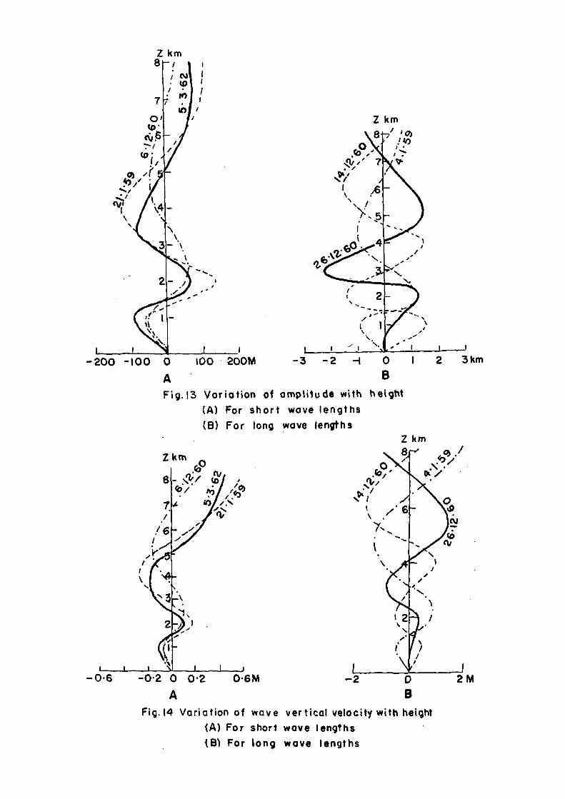
Fig. 13 Variation of amplitude with height

(A) For short wave lengths

(B) For long wave lengths

Fig. 14 Variation of wave vertical velocity with height

(A) For short wove lengths

(B) For long wave lengths

Fig. 15 Streamline displacement due to wave at levels of 2 , 4 , 6 & 8 km.

on 26.12.60 (12 Z)

(A) For longest wavelength L1 = 7 8 . 5 km

(B) For two wavelenths L1 = 7 8 . 5 km & L2= 11.2 km

Fig. 16 Profi le of f ( z ) = 2 for July 5 , 1961 for saturated a tmosphere .

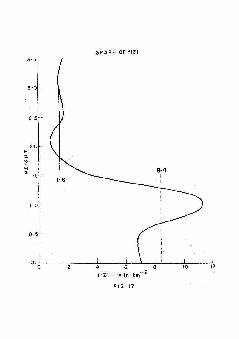
FIG. 17

FIG. 18 : 9 JAN 1967

OBSERVED WAVELENGTH IS 22 KM & COMPUTED

WAVELENGTH IS ALSO 22 KM ( D E 1970 )

FIG. 19 : 29 JAN. 1 9 6 7

OBSERVED WAVELENGTH IS 22 KM 8 COMPUTED

WAVELENGTH IS 20 .9 KM (DE 1970)

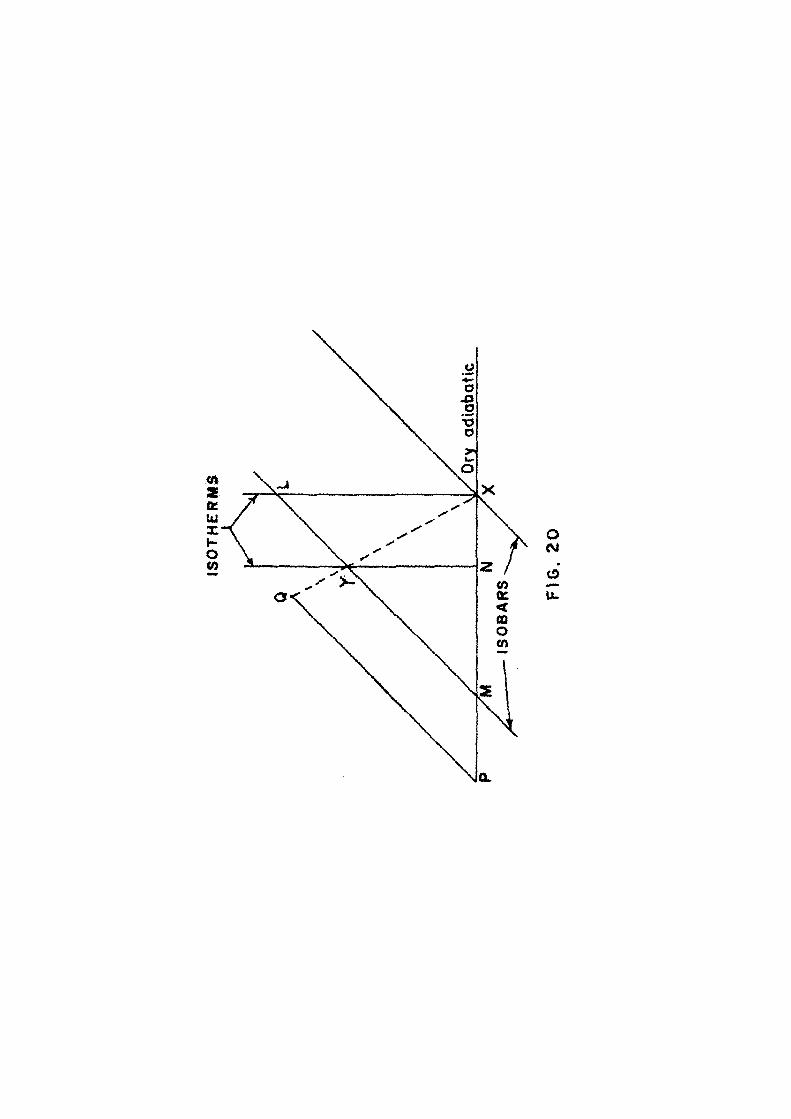
FIG

. 2

0

FIG. 2I

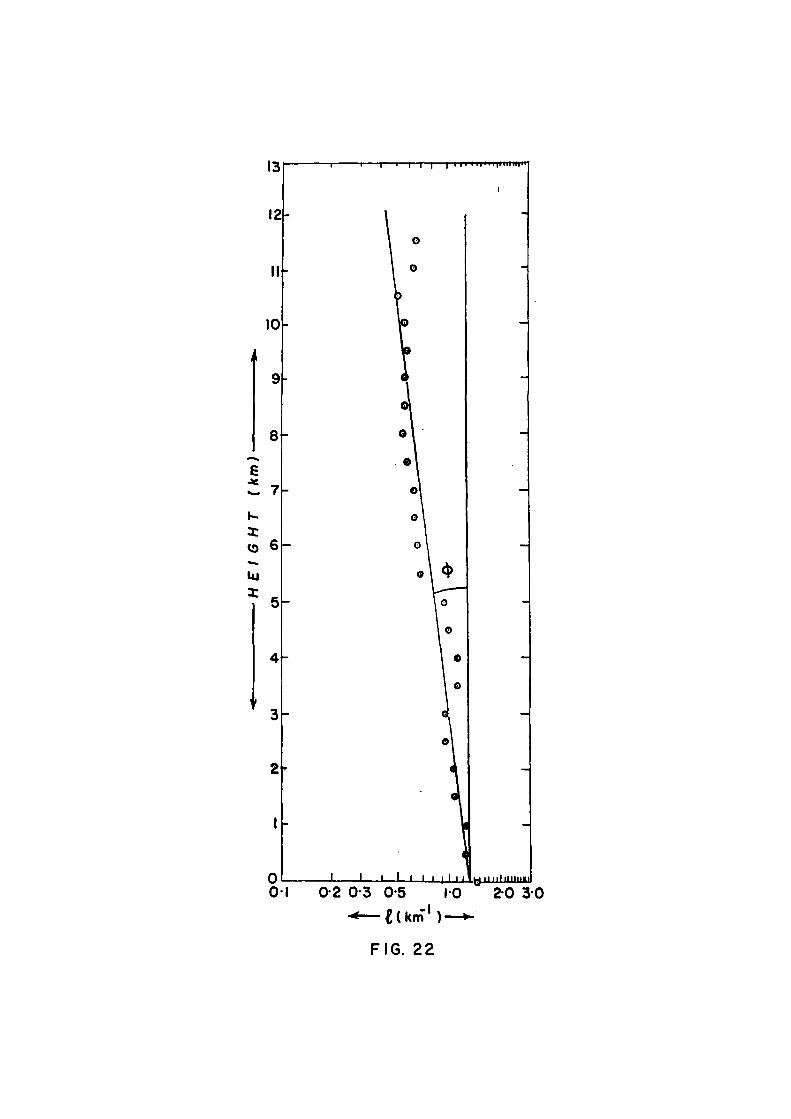
FIG. 22

FIG

. 23(a

)

FIG

. 23

(b

)

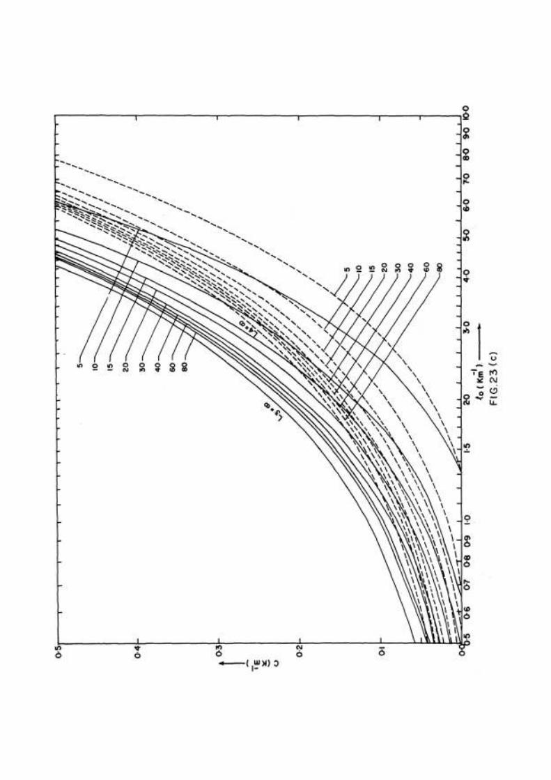
FIG

. 23

(c)

No.III-3.9 Discussion of Typical Synoptic Weather Situations: Southwest

Monsoon: Typical Situations over Interior Peninsula and

Coastal Andhra Pradesh - N.M. Philip, V. Srinivasan and

K. Ramamurthy.

No.III—4.1 Discussion of Typical Synoptic Weather Situations:

Weather over the Indian seas during the Post—Monsoon

Season - V. Srinivasan and K. Ramamurthy.

No.IV-13 Rainfall of India — P. Jagannathan.

No.IV-16 Microseisms and Weather - A.N. Tandon and S.N. Bhattacharya,

No.IV—17 Medium Range Forecasting - K.R. Saha and D.A. Mooley.

No.IV-18.1 On the Criteria for declaring the onset of the southwest

monsoon over Kerala — R. Ananthakrishnan, U.R. Acharya and

A.R. Ramakrishnan.

No.IV-18.2 Monsoons of India: Synoptic Features associated with onset of

Southwest Monsoon over Kerala — R. Ananthakrishnan,

V. Srinivasan, A.R. Ramakrishnan and R. Jambunathan.

No.IV-18.3 Some aspects of the "Break" in the Indian Southwest Monsoon

during July and August - K. Ramamurthy.

No.IV-18.4 Northeast Monsoon - V. Srinivasan and K. Ramamurthy.

No.IV-20 Evaporation - N. Ramalingam.

No.V-1 Techniques of High Level Analysis and Prognosis:

1. Organization and Methods of Analysis - P.K. Das,

N.C. Rai Sircar and D.V. Rao.

No.V-2 Techniques of High Level Analysis and Prognosis:

2. Prognostic Techniques and Assessment of Accuracy of

Forecasts - P.K. Das, N.C. Rai Sircar and D.V. Rao.