Electronic copy available at: http://ssrn.com/abstract=1876765

Indexing Executive Compensation Contracts∗

Ingolf Dittmann† Ernst Maug‡ Oliver Spalt§

April 26, 2013

Abstract

We analyze the efficiency of indexing executive pay by calibrating the standard modelof executive compensation to a large sample of US CEOs. The benefits from linkingthe strike price of stock options to an index are small and fully indexing all optionswould increase compensation costs by about 50% for most firms. Indexing has severaleffects with overall ambiguous impact; the quantitatively most important effect is toreduce incentives, because indexed options pay off when CEOs’ marginal utility is low.The results also hold if CEOs can extract rents and extend to the case of indexingshares.

JEL Classifications: G30, M52Keywords: Executive compensation, indexed options, relative performance evaluation, payfor luck

∗We thank Pierre Chaigneau, Jeff Coles (discussant at the CEAR workshop), Alex Edmans, Yaniv Grin-stein (WFA discussant), Wayne Guay, Zacharias Sautner, an anonymous referee, and seminar participantsat the Asian Finance Association meetings, the CEAR/Finance workshop on Incentives and Risk-Taking atGeorgia State University, the Conference on Executive Compensation and Corporate Governance in Rot-terdam, at Copenhagen Business School, Goethe University Frankfurt, HEC Montréal, HEC Paris, LondonBusiness School, London School of Economics, Maastricht University, the University of Michigan BusinessSchool, Tilburg University, University College Dublin, Vienna University of Economics and Business, and the2010 Western Finance Association Meetings. Ingolf Dittmann acknowledges financial support from NWOthrough a VIDI grant.†Erasmus University Rotterdam, P.O. Box 1738, 3000 DR, Rotterdam, The Netherlands. Email:

dittmann@ese.eur.nl. Tel: +31 10 408 1283.‡University of Mannheim, D-68131 Mannheim, Germany. Email: maug@bwl.uni-mannheim.de, Tel: +49

621 181 1952.§Tilburg University, P.O. Box 90163, 5000 LE, Tilburg, The Netherlands. Email: o.g.spalt@uvt.nl. Tel:

+31 13 466 3545.

Electronic copy available at: http://ssrn.com/abstract=1876765

“Investors should encourage equity-based plans that filter out at least some of the gainsin the stock price that are due to general market or industry movements. With suchfiltering, the same amount of incentives can be provided at a lower cost.” (Bebchukand Fried (2004), p. 190).“Options can easily be designed to make executives’ incentives more rational – so thatexceptional performers can earn greater returns than they would with standard options,while poor performers are appropriately penalized. How? Tie the price an executive paysfor stock when he exercises his options (...) to a broader market index.” (Rappaport,Wall Street Journal, March 30, 1999, p. 1).

1 Introduction

Standard principal-agent theory prescribes that managers should not be compensated on

exogenous risks, such as general market movements. Rather, firms should index pay and use

contracts that filter exogenous risks (e.g., Holmstrom (1979, 1982); Diamond and Verrecchia

(1982)). This prescription is intuitive and agrees with common sense: CEOs should only

receive exceptional pay for exceptional performance and “rational” compensation practice

should not permit CEOs to obtain windfall profits in rising stock markets. However, observed

compensation contracts are typically not indexed. Specifically, stock options almost never tie

the strike price of the option to an index that reflects market performance or the performance

of peers.1 Commentators often cite this glaring difference between theory and practice as

evidence for the inefficiency of executive compensation practice and, more generally, as

evidence for major deficiencies of corporate governance in US firms (e.g., Rappaport and

Nodine (1999); Bertrand and Mullainathan (2001), and Bebchuk and Fried (2004)). This

paper therefore contributes to the discussion about which compensation practices reveal

deficiencies in the pay-setting process.2

1Murphy (1999) reports that only one out of 1,000 firms in his sample had an indexed option plan. SeeMeulbroek (2002) for the case of one company that used indexed options. Other forms to use indexation forlimiting windfalls from strong stock market performance are also rare. For example, Bettis, Bizjak, Coles,and Kalpathy (2010) find that only 35 of the 983 firm-years in their sample use the stock market index or thestock performance of industry peers for performance-vesting conditions (see their Table 2, Panel D). Jenterand Kanaan (2008) show that CEO turnover becomes more likely after poor market or industry performance,which is inconsistent with the notion that firms shield CEOs’ human capital from market risk. We commentin Section 2 on the difference between indexing and relative performance evaluation; there is some evidencethat the latter does occur in practice.

2Bebchuk and Fried (2004) sparked a controversy on the efficiency properties of a range of compensationarrangements, which has yielded numerous surveys and policy proposals. See, e.g., Core and Guay (2010);Edmans and Gabaix (2009) and Weisbach (2007) for surveys.

1

Electronic copy available at: http://ssrn.com/abstract=1876765

This paper addresses the indexation of compensation contracts with a particular focus on

indexed options, which link the strike price to an index and are a central theme in the debate

about executive pay.3 We highlight two main contributions. First, we show analytically that

indexed options differ from conventional options in three important ways: (1) the underlying

asset of indexed options has a lower volatility; (2) the underlying asset does not earn a risk

premium and therefore has a lower drift rate; (3) indexing increases the strike price of the

option. We show that the first effect not only generates the familiar benefits from risk sharing,

but also improves incentives; a simple intuition for this effect is that reducing volatility

reduces the probability that in-the-money options expire out of the money and therefore

increases the option’s utility-adjusted delta. The latter two effects reduce incentives because

they implicitly raise the performance benchmark, reduce the probability that the option ends

up in the money, and therefore reduce the utility-adjusted deltas of options.4

Proponents of indexation often rely on the risk-sharing component of the first effect,

whereas more critical voices emphasize the third effect.5 The drift-rate effect is usually

neglected. By contrast, our analysis shows that a proper assessment of indexation needs to

look at the impact of all three effects jointly and weigh the advantages from (1) against the

disadvantages from effects (2) and (3). The efficiency of indexing stock options is theoretically

ambiguous and ultimately an empirical question.

Our second contribution is to calibrate the standard model used in the compensation

literature individually to each CEO in a large sample of US CEOs. Calibration allows us

to quantify the costs and benefits from indexing for each individual CEO, determine how

the different effects play out, and identify the cases in which indexing is beneficial. Our

calibration approach also reveals to what extent the trade-offs between the different effects

are the same for all CEOs. The central finding from our calibration analysis is that across3See Rappaport and Nodine (1999); Johnson and Tian (2000); Hall and Murphy (2000, 2002), and Be-

bchuk and Fried (2004)4There is a fourth effect, which is empirically of minor importance and therefore not emphasized here. It

implies that indexed options retain some exposure to market risk.5See the belief in “lower costs” in the opening quotes as an example for a focus on the first effect and

Murphy (2002) as a statement of the third effect.

2

the many different scenarios we consider, indexing creates either small savings or large costs.

In many empirically relevant cases indexed options provide incentives at a higher cost than

conventional options, which is in line with the skepticism expressed by Murphy (2002), but

contrary to widely held beliefs that the absence of indexation indicates poor governance. We

suggest that the absence of indexation can be explained based on the fundamental trade-off

between risk and incentives.

In our baseline case we analyze the full indexation of stock options under the assumption

that contracting is efficient and managers do not extract rents; in terms of our model, the

last condition implies that shareholders have to adjust base salaries to ensure that managers’

participation constraint remains satisfied. We find that full indexation of stock options

increases compensation costs by more than 50% on average in our baseline parameterization.

In dollar terms, average CEO pay would increase by $32.5 million ($1.5 million at the

median). Only about 15% of firms would benefit from indexing all options of the CEO. The

few firms that benefit from indexation are high-beta, high-risk firms that have CEOs with a

relatively high level of absolute risk aversion. For these firms the benefits from the reduction

in volatility (the first effect of indexed options discussed above), which improves incentives

as well as risk-sharing, outweigh the costs of reduced incentives from a stricter performance

hurdle (the second and third effect). In particular, a higher beta creates a larger scope to

reduce risk through indexation.

We extend our baseline setting in several dimensions. We first analyze partial indexation

and allow firms to optimally choose the proportion of stock options they wish to index.

Then the efficiency gains from indexation are non-negative by construction. For our baseline

parameterization firms would save 2.3% of compensation costs on average, which is less than

$1 million for the average CEO. Still, the adverse effects of indexation on incentives imply

that three quarters of the firms in our sample would optimally choose not to index their

CEOs’ options at all.

Our analysis shows that the indexation of stock options as proposed in the literature is

3

unwarranted in most cases, but leaves open whether alternative forms of indexation may still

be beneficial. We therefore examine two alternative forms of indexation in additional tests.

First, we analyze options on indexed stock. Indexed stock is a security that carries only the

firm-specific risk of the stock and has an expected return equal to the risk-free rate. At-the-

money options on indexed stock improve on indexed options, because options on indexed

stock avoid the implicit increase in the strike price (effect (3) above), and therefore provide

incentives more efficiently compared to indexed options, which are out of the money and

have a lower delta. We confirm that options on indexed stock are more effective. However,

the gains from using them are still limited, because of the adverse effect of the reduction

in the drift-rate of the underlying asset (effect (2) above); more than 40% of firms would

optimally use only conventional, non-indexed options rather than options on non-indexed

stock.

Second, we analyze indexed stock itself. Indexing stock does not involve any of the

complications associated with the strike price we encountered with indexed options or with

options on indexed stock. Hence, we expect indexed stock to perform better than any of

the options we study. Interestingly, this conjecture is confirmed, but the gains are not large:

Fully indexing all restricted shares leads to efficiency gains near zero, whereas optimal partial

indexation of stock leads to gains that are about 25% to 30% larger than those observed for

the partial indexation of options. In absolute terms, savings are always small, because the

volatility effect and the drift-rate effect carry over from the case of stock options to shares.

The analysis of indexed stock and options on indexed stock allows us to isolate the different

effects we highlight above and to compare securities with different exposures to these effects.

This comparison is one of the contributions of this paper.

Finally, we adopt the perspective of the rent-extraction view (e.g., Bebchuk and Fried

(2004)). This step of the analysis is important because proponents of the rent-extraction

view may not agree with the presumption that shareholders have to compensate CEOs for

the loss associated with exchanging valuable conventional options for much less valuable

4

indexed options. We model rent extraction in our context by dropping the assumption that

CEOs’ outside options are binding. Effectively, we ask which contracts would be optimal

if firms only want to provide a given level of incentives, but do not need to be concerned

about retaining the CEO. In this framework we ask whether indexation is an appropriate

strategy for shareholders to recapture rents. The analysis shows that for about half of all

CEOs, indexation does not help with recovering rents. Indexation would still increase CEO

pay levels by more than 20% on average if firms were required to fully index stock options.

Optimal partial indexation leads to cost savings of just under 8% of compensation costs.

The intuition for these results is that indexing leads to inefficient incentive provisions for the

same reasons as in the efficient contracting case.

We conduct all our analyses for a range of different parameterizations and subject the

results to several robustness checks. Specifically, our findings are not driven by our treatment

of the CEO’s investment in the stock market as exogenous and are also not attributable to

the fact that stock market risk is associated with a risk premium.

The model we use is a standard principal-agent model with CRRA utility and lognormal

stock prices. This modeling strategy has become standard in much of the compensation

literature and our results can therefore be compared directly with previous work.6 The

impact of the three main effects of indexing options is theoretically ambiguous and depends

on parameter values, which makes calibrations at the individual CEO level the research

strategy of choice. Our approach is also fairly general and does not require additional

assumptions about functional forms other than concavity of the production function and

convexity of the effort cost function of the CEO.7 However, two assumptions are necessary

to ensure tractability. First, we do not endogenize the balance between stock and options

and only discuss to what extent it is optimal to index the shares and options in observed

contracts. The focus on observed contracts is necessary as the CRRA-lognormal setup would6See e.g., Lambert, Larcker, and Verrecchia (1991); Hall and Murphy (2000, 2002); Himmelberg and

Hubbard (2000); Hall and Knox (2004), and Oyer and Schaefer (2005).7We still require additivity in the utility function. See, e.g., Edmans, Gabaix, and Landier (2009) for a

model that uses a multiplicative modeling approach.

5

hardly feature options as part of the optimal contract (Dittmann and Maug (2007)). Second,

we do not allow for changes in the level of effort and hold it fixed at the level implied by

the observed contract. In Section 7 we argue why we believe the effects we identify to be

robust and why we believe the benefits from indexation to be always limited, if not outright

negative, in non-standard setups that overcome these limitations of our approach.

The intuitive appeal of indexation is closely related to Holmstrom’s (1979) seminal work

on the informativeness principle. The informativeness principle implies that there exists an

optimal contract that filters all exogenous risks. However, this optimal contract will generally

be a highly non-linear function, and Holmstrom himself observes that filtering risks does not

take the simple form of subtracting an index from the output measure except for some special

cases (Holmstrom (1982), p. 377). Nothing in our work contradicts the informativeness

principle. Instead, we follow the compensation literature and analyze observed contracts

that can be constructed from shares and stock options, which are empirically more relevant,

but not necessarily optimal. Whether indexing these contracts improves efficiency is an

open question that cannot be resolved by appealing to the informativeness principle. Our

calibrations show that indexing options moves piecewise linear contracts further away from

efficiency. Furthermore, other simple forms of indexation are more beneficial, even though

they also fall short of filtering all exogenous risks. The informativeness principle can therefore

provide only limited guidance for the optimal design of observed, piecewise-linear contracts.

2 Discussion of the literature

Several contributions in the literature address the glaring gap between the prescriptions of

standard economic models and observed compensation practice within the efficient contract-

ing paradigm. First, relative performance evaluation might induce unwanted incentives to

intensify industry competition (e.g., Aggarwal and Samwick (1999)); indexed options might

provide incorrect incentives for entering or exiting industries (e.g., Dye (1992); Gopalan,

Milbourn, and Song (2010)); indexed options might be tax inefficient (e.g., Göx (2008));

6

indexed options could be replicated by managers through appropriate rebalancing of their

own portfolio between the benchmark portfolio and the riskfree asset if such rebalancing

would be costless (e.g., Garvey and Milbourn (2003); Jin (2002); Maug (2000)). Our anal-

ysis complements this previous literature on the lack of indexation, but we abstract from

the additional channels identified in that literature, which biases our analysis towards find-

ing larger improvements from indexation. Most importantly, we show that adding specific

assumptions about the strategic context of the firm, the tax code, or the CEO’s trading

opportunities is not necessary to explain the absence of indexing.

Our work is also related to a number of papers that discuss the indexation of options, or

design features of stock option more broadly. Rappaport and Nodine (1999) and Bebchuk

and Fried (2004) both propose indexed options, but rely on intuitive arguments and nu-

merical examples. None of them discusses the consequence of indexation on incentives for

risk-averse CEOs. Hall and Murphy (2000, 2002) and Ross (2004) provide important insights

on changes in the strike price, but do not explicitly analyze indexing and do not consider

the countervailing volatility effect. Murphy (2002) argues that indexed options have a low

probability of being in the money and argues that these options are inferior to in-the-money

options, but links his argument to the subjective value of options to CEOs, i.e., to their

participation constraint, and not to their incentives, which we show is the critical ingredient.

The paper that is perhaps closest to our is Chaigneau (2012) who endogenizes the struc-

ture of pay but works in a framework without risk-aversion and with normally distributed

stock prices. Chaigneau (2012) does not calibrate his model to observed CEO compensation

contracts.

Our paper also contributes to the broader literature on relative performance evaluation

(e.g., Antle and Smith (1986); Bertrand and Mullainathan (2001); Garvey and Milbourn

(2003)). It is important to note that the empirical design used in the literature on relative

performance evaluation addresses a somewhat different question than we do, because it an-

alyzes ex post payouts, which include changes over time in fixed salaries as well as in the

7

value of new stock and option grants. These dynamic considerations are absent from static

theoretical models, which predict that benchmarks are built into ex ante contracts. While

all forms of ex ante indexation would be reflected in the regressions used in the empirical

literature on relative performance evaluation, the converse is not true: In fact, the evidence

on relative performance evaluation may not reflect indexation of ex ante contracts at all

(see footnote 1). For example, if boards regard CEOs’ performance relative to their peers

as information about CEOs’ talent, superior performance relative to a benchmark reveals

the CEO’s superior abilities and boards will increase pay as they update their assessment

of the CEO’s talent – a dynamic consideration that is unrelated to the design of ex ante

contracts, which are supposed to provide efficient incentives. Alternatively, CEOs and com-

pensation committees may use benchmarking opportunistically to support claims for higher

compensation (Faulkender and Yang (2010)). In our discussion we therefore distinguish two

definitions. We use the term indexation narrowly to refer to the benchmarking of ex ante

contracts against an index with the intent to remove pay for luck. By contrast, we use

the term relative performance evaluation more broadly, so that it also includes the ex post

adjustment of fixed compensation and bonus payments.

3 Research design

We consider a standard principal-agent model in the spirit of Holmstrom (1979). In this

section, we develop the model, present our calibration approach, and explain the construction

of our data set.

3.1 The model

The CEO (agent) provides costly and unobservable effort on behalf of shareholders (princi-

pal). At the beginning of the period (time 0) shareholders propose a contract to the CEO.

When the CEO accepts the contract, she exerts effort e during the contracting period, and

8

this effort positively affects the end-of-period stock price PT , where T denotes the length of

the contracting period. As effort is not observable, the contract depends only on the stock

price PT and on the stock market index MT , and generates a payoff πT to the agent at the

end of the period. We denote the beginning of period stock price by P0 and normalize the

value of the index at time zero so thatM0 = 1; MT therefore denotes the return on the stock

market index.

The CEO’s utility. The CEO’s wealth that is not invested in her own firm is denoted by

W0. For brevity we refer to W0 as non-firm wealth. A fraction ω ∈ [0, 1] of this wealth is

invested in the market portfolio and yields a return per dollar invested of MT at the end of

the period, while the remaining wealth is invested at the risk-free rate rf . We treat ω as an

exogenous parameter in most of our analysis. The CEO also owns nSU unrestricted shares.

We treat unrestricted shares as part of the CEO’s portfolio and not as a part of the contract

with the firm, whereas restricted shares are a part of the contract. We assume that these

are not part of the contract negotiations, but that they contribute to her incentives and her

wealth. The CEO’s end-of-period wealth therefore is

WT = W0((1− ω)erfT + ωMT

)+ nSUPT + π̃T , (1)

where π̃T is the CEO’s income from the employment with the firm. The CEO’s utility is

additively separable in end-of-period wealth and effort, i.e., u(WT , e) = U(WT )−C(e), where

C(e) is increasing and convex. The CEO is risk-averse in wealth with constant relative risk

aversion (CRRA):

U(WT ) = 11− γW

1−γT , (2)

where γ is the coefficient of relative risk aversion (if γ = 1, we define U(WT ) = ln(WT )). We

use constant relative risk aversion because this assumption has become the benchmark model

in the compensation literature. The CEO’s outside option when she declines the contract is

U.

9

Contracts and shareholders’ optimization. We consider piecewise linear contracts

that consist of a fixed salary φ, the number of restricted shares nSR, and the number of

options nO, where we express nSR and nO as a proportion of all outstanding shares. Moreover,

a proportion ψ ∈ [0, 1] of the options is indexed, so that the CEO’s compensation is

π̃T =φerfT + nSRPT + nO(ψOidx

T + (1− ψ)max {PT −K, 0}).

Here, K is the strike price of the option and OidxT is the payoff of an indexed option. The

base salary is paid at the beginning of the contracting period and invested at the risk-free

rate rf . The firm has access to capital markets, so the cost to the firm from granting the

contract is the time zero market value of the securities granted to the CEO, which we denote

by π0. Shareholders’ objective is therefore to minimize π0:

min π0 = φ+ nSRP0 + nO (ψJT + (1− ψ)BS) (3)

In (3), BS stands for the Black-Scholes value of options and JT denotes the value of indexed

options according to the valuation formula of Johnson and Tian (2000), which we provide

below. Shareholders’ problem is to minimize the market value of compensation costs π0

subject to the two constraints that (1) the CEO accepts the contract and that (2) she will

exert the desired effort level e∗. Shareholders therefore minimize π0 subject to:8

E [u (WT , e∗)] ≥ U, (4)

d

deE [u (WT , e

∗)] = 0. (5)

8For the incentive compatibility constraint, we assume that the first-order approach is satisfied. A suffi-cient condition is that the optimization problem is globally concave, and this is the case if the cost functionC(e) is sufficiently convex and the production function P0(e) is sufficiently concave. Dittmann and Maug(2007) numerically check whether the optimal contract induces the CEO to choose less effort than the ob-served contract. We do not follow their approach here, because our main result is that the improvement ofthe optimal contract over the observed contract is only marginal, so that we do not suggest that firms shouldswitch to the optimal contract.

10

Stock price and market index. We assume that the end-of-period stock price PT is

lognormally distributed,

PT = P0 (e) exp{(

µP −σ2P

2

)T + uPσP

√T

}, (6)

where P0 (e) is an increasing and concave function in effort e, µP is the expected annual total

return (dividends plus capital gains), σP is the annual standard deviation of stock returns,

uP is a standard normal random variable, and T denotes the length of the contracting period.

Similarly, the end-of-period value of the stock market index MT is lognormally distributed

(recall that M0 = 1):

MT = exp{(

µM −σ2M

2

)T + uMσM

√T

}. (7)

The definitions of µM , and σM are analogous to those for PT . The actions of the CEO do

not affect the value of the index. Furthermore, uP and uM are correlated with a coefficient

of correlation ρ. The CAPM holds, so β = ρ σP

σMand9

µP = rf + β (µM − rf ) . (8)

Indexed stock. For ease of exposition, we discuss indexed stock first and then introduce

indexed options. Conventional stock earns a return PT/P0 and an expected return equal

to µP . By contrast, indexed stock filters the systematic component and earns an expected

return equal to the risk-free rate. We construct indexed stock from the residual between the

actual stock price PT and the expected stock price conditional on the market index. Johnson

and Tian (2000) show that the expected value of PT given the value of the index MT is:

E [PT |MT ] = HT ≡ P0MβT e

ηT , (9)9Compared to the setup of Johnson and Tian (2000), we ignore the possibility of deviations from the

security market line here. In their notation, we set α = 0.

11

where

η ≡ (1− β)(rf + 1

2ρσMσP). (10)

Here, HT represents the systematic component of stock returns. Consider the simple case

with β = 1. Then we have η = 0 and HT = P0MT , i.e., the expected stock price at time

T conditional on the market index equals the current stock price, multiplied by the return

on the market. If β = 0, then ρ = 0 and HT = P0exp (rfT ); the market index provides

no information for predicting the stock price in this case. With the help of this definition

we define the return on indexed stock as (PT/HT ) exp (rfT ) and normalize the price of

an indexed share by setting it equal to the price of one conventional share at t = 0, i.e.,

P idx0 = P0. Then the price of an indexed share at time T equals

P idxT = P0

PTHT

exp (rfT ) . (11)

In the appendix we show that the terminal value of indexed stock P idxT can be written anal-

ogously to (6) as:

P idxT = P0exp

{(rf −

σ2I

2

)T + uIσI

√T

}. (12)

where: σI = σP√

1− ρ2, (13)

uI = (uPσP − uMρσP ) /σI . (14)

The standard normal random variable uI reflects the firm-specific variation in stock returns

and is uncorrelated with uM . Firm-specific risk is measured by σI . It is useful to rewrite the

stock price PT asPT = b P idx

T MβT ,

where b = exp ((η − rf )T ) .(15)

Hence, the price of a conventional share can be expressed as the product of the price of an

indexed share and the market-related component bMβT .

12

Payoffs and valuation of indexed options. We follow Johnson and Tian (2000) and

define the payoff of indexed options as

OidxT = max {PT −HT , 0} . (16)

Hence, the strike price of an indexed option is equal to the expected value of the stock price

conditional on the market index. Indexed options are in the money only if the return on the

firm’s stock beats the market index. For example, if the market moves up by 5%, then a

CEO in a firm with β = 1 will only receive a payoff from indexed options if the firm’s stock

appreciates by more than 5%. We use the formula of Johnson and Tian (2000) to value

indexed options at time t = 0 and denote the corresponding “Johnson-Tian” value of these

options by JT. This value is given by:

JT = e−dT[P0N(didx1 )− P0N(didx2 )

], (17)

where: didx1 = σI√T

2 , didx2 = −σI√T

2 . (18)

3.2 Calibration

We use the calibration method introduced by Dittmann and Maug (2007).10 We denote

the observed contract by (φd, ndS, ndO, ψ = 0) (“d” stands for “data”) and assume that the

observed contract implements the desired effort level e∗ and does not leave the CEO with a

rent. We define the utility-adjusted pay-for-performance sensitivity UPPS as:11

UPPS(φ, nS, nO, ψ) ≡ d

dP0E [U(WT (φ, nS, nO, ψ))] . (19)

10See also the technical document by Dittmann, Zhang, Maug, and Spalt (2011), which explains thetechnical aspects of their calibration algorithm in more detail.

11Note that for the case of risk neutrality where V (WT ) = WT , UPPS reduces to the more familiarpay-for-performance sensitivity, which in our case is equal to nS + nO(1− ψ)N(d1) + nOψN(dindx

1 ); N(d1)and N(dindx

1 ) denote the delta of conventional options and indexed options, respectively.

13

We focus mostly on the indexation of options and discuss the indexation of restricted shares

later. We do not endogenize the balance between restricted stock and options of the con-

tract. Dittmann and Maug (2007) show that a CRRA-lognormal model as we analyze here

suggests significant efficiency gains from replacing options with stock and we do not wish

to confound the efficiency gains from indexation with the efficiency gains from changing the

balance between stock and options. Hence, whenever we analyze the indexation of options

we satisfy the incentive compatibility constraint (5) by replacing conventional options with

an appropriate number of indexed options, while fixing the number of restricted and unre-

stricted shares at their observed levels. The CEO and shareholders therefore bargain over

fixed salary φ, the number of options nO, and the proportion ψ of options that are indexed.

(We sometimes use the subscripts ’S’ and ’O’ on ψ to refer to the degree of indexation of

shares and options, respectively, but omit the subscript if the meaning is unambiguous.)

Then the optimization problem (3) to (5) can be rearranged as follows:12

min{φ,nO,ψ}

E [π0(φ, nO, ψ)] (20)

subject to:

E [U (WT (φ, nO, ψ))] ≥ E[U(WT

(φd, ndO, 0

))], (21)

UPPS(φ, nO, ψ) ≥ UPPS(φd, ndO, 0), (22)

ψ ∈ [0, 1] . (23)

Hence, we search for the cheapest contract that provides the CEO with at least the same

utility as the observed contract and that induces at least the same level of effort as the

observed contract. If indexing is important, a contract with ψ > 0 should be optimal and12We use similar steps to Dittmann and Maug (2007) and Dittmann, Maug, and Spalt (2010) here. Note

that this step effectively substitutes out the production function P (e) and the cost function C(e) and permitsus to proceed without specifying their functional forms. As a consequence, we can only analyze the structureof the contract and not the overall level of pay, which is given from the observed contract.

14

significantly cheaper than the observed contract.

We can completely parameterize the expressions in (21) and (22) by determining appro-

priate values for the contract parameters φd, ndS, and ndO, the parameters of the stock price

processes (6) to (8), and the CEO’s risk aversion parameter γ.

In our baseline setting, we take the CEO’s exposure to the stock-market ω as exogenous

and fixed. There are two reasons for this step, one practical and one conceptual. On the

practical side, fully endogenizing ω would render the problem intractable.13 We will partially

endogenize ω later, however, and show that we can come close to endogenizing ω; our

conclusions are not affected. On the conceptual side, fixing ω is a conservative assumption

that biases us towards finding larger savings from indexation and therefore against our

conclusions. In fact, the literature on the homemade-indexing argument points out that

the benefits from indexing may in some instances be completely annihilated if the CEO

could choose her investment in the stock market ω optimally. Then the CEO would remove

any excess exposure to stock market risk herself and indexation would yield no further

improvements (Garvey and Milbourn (2003); Jin (2002), and Maug (2000)).

3.3 Data

We use the ExecuComp database to construct CEO contracts at the beginning of fiscal year

2006. We first identify all persons in the database who were CEO during the full year 2006

and executive of the same company in 2005. We calculate the base salary φ as the sum of

salary, bonus, and “other compensation” from 2006 ExecuComp data and take information

on stock and option holdings from the end of fiscal year 2005 . We regard the data for 2006

as more representative for our purposes as subsequent years were affected by the financial

crisis.13There is no closed-form solution of the CEO’s portfolio problem and we would therefore have to work

with a nested optimization problem where the firm first chooses the optimal contract and the CEO thenadjusts her private portfolio accordingly. Also, the firm would have to anticipate the CEO’s actions, so thatthe inner optimization problem would have to be solved at every point where the outer optimization problemis evaluated. It is unlikely that such a model can be solved in a reasonable amount of time with today’scomputing power.

15

We estimate each CEO’s option portfolio with the method proposed by Core and Guay

(2002) and then aggregate this portfolio into one representative option. We set the repre-

sentative option to be at the money and calculate the number of representative options ndO

and the maturity T of the representative option so that they have the same Black-Scholes

value and the same option delta as the estimated option portfolio.14 In this step, we lose five

CEOs for whom we cannot numerically solve this system of two equations in two unknowns.

We take the firm’s market capitalization P0 from the end of 2005. While our formulas

above abstract from dividend payments for the sake of simplicity, we adjust option values

for dividends in our empirical work and use the dividend yield d from 2005. We estimate the

firm’s stock return volatility σ and CAPM−β from monthly CRSP stock returns over the

five fiscal years 2001 to 2005 and drop all firms with fewer than 45 monthly stock returns.

The risk-free rate is set to the U.S. government bond yield with five-year maturity from

January 2006.

We estimate non-firm wealthW0 of each CEO from the ExecuComp database by assuming

that all historic cash inflows from salary and the sale of shares minus the costs of exercising

options have been accumulated and invested year after year at the one-year risk-free rate.

We assume that the CEO had zero wealth when she entered the database, which biases our

estimate downward, and that she did not consume since then, which biases our estimate

upward. To arrive at meaningful wealth estimates, we discard all CEOs who do not have a

history of at least five years for 2001 to 2005 on ExecuComp. During this period, they need

not be CEO. This procedure results in a data set with 755 CEOs.

Table 1 provides an overview of our data set. The median CEO in the sample owns 0.25%

of the stock of his company, of which 0.02% is restricted and 0.23% is unrestricted. Median

option holdings are on 1.02% of the company’s stock. Median base salary is $1.04m, and the14We take into account the fact that most CEOs exercise their stock options before maturity by multiplying

the maturities of the individual option grants by 0.7 before calculating the representative option (see Huddartand Lang (1996) and Carpenter (1998)). In these calculations, we use the stock return volatility fromExecuComp and, for the risk-free rate, the U.S. government bond yield with 5-year maturity from January2006. Data on risk-free rates were obtained from the Federal Reserve Board’s website. For CEOs who donot have any options, we set T = 7 (10-year maturity multiplied by 0.7) as this is the typical maturity fornewly granted options.

16

median non-firm wealth is $13.49m.

The only parameter in our model that we cannot estimate from the data is the manager’s

coefficient of relative risk aversion γ. We use γ = 2 as a baseline case for most of our analysis

and also report results for γ = 1 and γ = 3.15

Murphy (1999) reports that in a sample of 627 firms that granted stock options to their

executives in 1992, only one firm used indexed options. Since ExecuComp does not report

indexing, we therefore assume that all stock and options in the observed contract are not

indexed. This assumption implies that we might overstate the potential efficiency gains from

indexing.

Indexing should not be confused with performance vesting. In recent years, more and

more option grants do not vest automatically after a certain time period but only when some

performance criterion (e.g., a minimum return on assets) has been achieved (see, e.g., Bettis,

Bizjak, Coles, and Kalpathy (2010)). Note also that some bonus schemes like phantom stocks

or bonuses that depend on the performance of a peer group constitute relative performance

pay (see Murphy (1999)). By treating bonuses as fixed salary, we do not include these

features in our stylized observed contract.

4 Full indexation of options

In this section we present the core of our analysis and investigate the costs and benefits on

fully indexing CEOs’ stock options. We first analyze the optimization problem (20) to (23)

with the provision that options are fully indexed (ψ = 1).15Different strands of the literature use different values of relative risk aversion and there is no consensus

on this subject. Ait-Sahalia and Lo (2000) survey the research on this topic, which supports values between0 and 55. The macroeconomic literature typically uses higher values (see Campbell, Lo, and MacKinlay(1997), chapter 8, for a survey and discussion). The compensation literature often uses lower values. Forexample, Murphy (1999) uses 1, 2, and 3, and Hall and Murphy (2002) use 2 and 3. Dittmann, Maug, andSpalt (2010) calibrate a loss-aversion model and show that it fits compensation data well. The degree ofrelative risk-aversion implied by their analysis varies between 0.2 and 1.

17

4.1 Result 1: Full indexation is costly

Table 2 shows the results for three values of the coefficient of relative risk aversion γ (1,

2, and 3) that have been considered in the literature (e.g., Hall and Murphy (2002)). For

each value of γ, the table provides the results for five levels of the proportion ω of CEO

non-firm wealth that is invested in the stock market. The table reports the means of the

base salary φ and of option holdings nO in the optimal contract. Finally, we report the

efficiency gains S from recontracting. We first calculate the costs of the observed contract

πd and the cost of the optimal contract predicted by the model, π∗. These estimates are

obtained from evaluating the costs of the contract π0 from (3) for the parameters of the

observed contract and for the optimal contract, respectively. Efficiency gains are defined as

the difference between these costs scaled by πd, so S = (πd − π∗)/πd (“S” for “savings”).

Our numerical routines do not converge for all observations and all parameterizations. The

number of observations in Table 2 therefore varies slightly.

Our first important result is that compensation costs increase dramatically for plausible

parameterizations of our model. We use γ = 2 and ω = 0.5 as our baseline case, i.e.,

we assume that CEOs invest 50% of their wealth in the stock market. Negative savings

S indicate an increase in compensation costs. Hence, for our baseline case, compensation

costs increase by 55.65% on average. For many parameterizations the average increase

in compensation costs exceeds 50%. There is significant cross-sectional variation and the

distribution is skewed and becomes more skewed for higher levels of risk aversion: for higher

levels of risk aversion, the median cost increase is lower, whereas the average cost increase

from indexation is larger. The proportion of firms that benefit from full indexation also

increases with risk aversion from 5.90% for γ = 1 to 27.27% for γ = 3 (always for ω = 0.5).

The remaining part of this section analyzes these puzzling findings in more detail. Table

2 offers important clues from comparing fixed compensation φ and the number of options nO

for indexed contracts with those for observed contracts. For our baseline case, the number

of options increases from an average of 1.49% in terms of the number of outstanding shares

18

for the observed contract (see Table 1) to 3.40% for the indexed contract. Hence, one

conventional option is replaced on average by 2.29 (=3.40/1.49) indexed options to maintain

incentives (UPPS from equation (19)) at the same level as in the original contract, which

indicates that one indexed option provides substantially lower incentives compared to one

conventional option. Similarly, base salaries increase from an average of $1.616 million to

an average of $3.051 million, an increase of 89%. This observation shows that managers

value the higher number of indexed options much less than the conventional options from

the original contract they give up. Both findings are important for the following discussion.

We observe that the number of CEOs for whom our algorithm converges decreases with

risk aversion. The numerical problems hide an underlying problem from incentivizing and

compensating CEOs with indexed options, because the algorithm does not converge for those

CEOs who do not obtain sufficient incentives from indexed options so that the incentive

compatibility constraint cannot be satisfied for any value nO ≤ 1. Hence, if we would

permit the number of indexed options to exceed 100% of the outstanding shares, then the

distributions reported in Table 2 would become even more skewed and indexation would

become even less desirable.

4.2 Result 2: Indexation destroys incentives

The main result from the previous section is that full indexation makes compensation more

costly for the large majority of firms. We analyze the reasons for this finding by decomposing

the savings from indexation in two steps. In the first step, we fix option holdings at their

observed level (nO = ndO). The algorithm then minimizes objective (20) only subject to the

participation constraint (21) and omits the incentive compatibility constraint (22). This

step allows us to isolate the benefits from improved risk-sharing, i.e., the benefits we could

obtain if indexation would have no impact on incentives. We refer to these gains as “gross

efficiency gains.” The resulting contract has costs πG and generates efficiency gains SG ≡(πd − πG

)/πd. In the second step we compute the efficiency gains from restoring incentives,

19

SI = S − SG, which is a measure of the effectiveness of indexed options as instruments to

provide incentives. These additional savings result from a change in the number of options

and a related adjustment in base salary. After the second step the contract simultaneously

satisfies the participation constraint (21) as well as the incentive compatibility constraint

(22).

The first column of Table 3 shows the gross efficiency gains SG, the gains from restoring

incentives SI , and the total efficiency gains S as percentages of the costs of the original

contract πd from fully indexing all options. We perform the calculations for three different

parameterizations. The table reports a further breakdown on which we comment below.

Gross gains from indexing SG equal 13.2% of compensation costs for the baseline param-

eterization with γ = 2 and ω = 0.5. Hence, if firms could simply enjoy the benefits from

improved risk-sharing by replacing each conventional option with an otherwise identical in-

dexed option without paying any attention to incentive effects, then compensation costs

would decline by 13.2%. In unreported results we find that these gains increase with risk

aversion, which is intuitive because improved risk sharing matters more if the risk premium

paid to the CEO is larger. In the second step, the model increases the number of options

so that the indexed options generate the same incentives as the conventional options in the

original contract. The resulting increase in compensation costs is economically significant,

with 70.8% for the baseline scenario. Hence, the gains from risk-sharing are more than out-

weighed by the losses from less efficient incentive provision. Costs from restoring incentives

are higher for lower values of ω. Table 3 reports the changes in incentives as ∆UPPS in

the last line of each panel. For the baseline parameterization, incentives decline by 9.8%

compared to the original contract if options are fully indexed. This is in direct contrast to

the view that “the same amount of incentives can be provided at a lower cost”, expressed in

the opening quote. In fact, the results in Table 3 show that indexed options are inferior to

standard options for most firms precisely because indexation destroys incentives.

Figure 1 illustrates the effects from the previous discussion by showing the net efficiency

20

Figure 1: Efficiency gains for an example CEOThis figure shows total savings, S, gross savings SG, and the savings from restoring incentivesSI as a function of the degree of indexation ψ for an example CEO from our sample. ThisCEO has the following parameters: β = 1.5, φd = $1.5m, nO = 1.6%, and W0 = $43m. Theoptimal degree of indexation for which savings are maximized is ψ∗ = 35% and savings atthis degree of indexation would be S = 3.03%.

‐60

‐50

‐40

‐30

‐20

‐10

0

10

20

30

0 0.1 0.2 0.3 0.4 0.5 0.6 0.7 0.8 0.9 1

Savings (%)

Degree of Indexation

S

SG

SI

gains S and their two components, SG and SI , as a function of the degree of indexation ψ.

The figure repeats our procedure for a grid of exogenously fixed values ψ ∈ [0, 1] for a typical

CEO in our sample. Several findings emerge. First, full indexation would be optimal if risk-

sharing would be the only objective, since SG is maximized for ψ = 1. The resulting savings

would be substantial, which explains the intuitive appeal of indexed options. Second, and

most importantly, indexation destroys incentives for all values of ψ. This effect is especially

pronounced for high degrees of indexation. Third, for full indexation, the savings from

improved risk-sharing are outweighed by the increased costs from restoring incentives, so

that the net effect S is negative. Finally, the figure suggests that net benefits S can be

slightly positive with partial indexation for sufficiently low ψ’s. This is exactly what we find

if we endogenize ψ (see Section 5.1 below).

21

4.3 Result 3: The performance benchmark of indexed options is

too strict

The difference between indexed options and conventional options. In the next

step of our analysis we study which aspect of indexation makes indexed options less efficient

for providing incentives to CEOs. Recall from (15) that we can rewrite the stock price as

PT = P idxT bMβ

T , where P idxT is the price of an indexed share and bMβ

T is a function of the

systematic component of the stock price defined in (15). Similarly, the strike price HT of an

indexed option can be rewritten using (15) as

E [PT |MT ] = HT = P0exp(rfT )bMβT . (24)

We can now rewrite the payoff of one indexed option given in (16) by using (24) and (15) as:

OidxT = max(PT −HT , 0) = bMβ

Tmax(P idxT − P0exp {rfT} , 0

). (25)

A number of observations emerge from (25). First, the payoff of an indexed option can be

written as the payoff of options on indexed stock P idxT ; indexed stock has a drift rate equal

to the risk-free rate rf and is only subject to firm-specific risk σI . Recall that we normalize

indexed shares so that their price at time t = 0 equals that of conventional shares. Second,

indexed options are out of the money; because their strike price equals P0exp(rfT ) > P0.

Third, and finally, the payoff OidxT of one indexed options equals bMβ

T options on indexed

stock, where bMβT reflects the component of the stock price PT that is related to the stock-

market index MT . The last step shows that indexing options does not fully insure CEOs

against fluctuations in the market index. Full insurance would require that the option payoff

is independent of the stock market index, and therefore of bMβT . Intuitively, doubling the

market index doubles the strike price of the option and the stock price, but thereby it also

doubles the difference between the stock price and the strike price; it should hold it constant

22

to achieve full insurance.16

We apply these insights by providing a further decomposition of the incentive and risk-

sharing effects in Table 3. The point of departure are the conventional options. We then go

through the following sequence of steps:

1. Reduce the volatility of the underlying asset from σP to σI . We refer to the impact of

this change as the volatility effect.

2. Reduce the drift rate of the underlying asset from µP to rf . We refer to the impact

of this change as the drift-rate effect. This step together with the previous step re-

places an at-the-money option on conventional stock with terminal value PT with an

at-the-money option on indexed stock. These options have a terminal payoff equal

max{P idxT − P0, 0

}. For brevity, we refer to these options as options on indexed stock.

3. Increase the strike price from P0 to P0exp(rfT ). We refer to the impact of this change

as the strike-price effect.

4. Replace each option on indexed stock by bMβT such options. This effect reintroduces

market exposure into the contract and we therefore label it the market-exposure effect.

These four steps together transform one conventional option into one indexed option. Each

step is associated with one effect, which allows us to calculate the impact of this effect sepa-

rately, holding all else equal. We perform these calculations separately for the gross savings

from risk-sharing SG, the savings from restoring incentives to their original level, SI , the total

savings from indexation, S, and for the change of incentives, ∆UPPS. For the calculations

of SG and ∆UPPS we only adjust fixed compensation so that the CEO’s participation con-

straint remains satisfied. For the calculations of SI and S we adjust the number of options

as well as fixed compensation to satisfy the incentive compatibility constraint.16Consider an indexed option with a strike price of 8 on stock with a current price of 10 when the index

value equals 100. Doubling the index value to 200 implies that the strike price and the stock price bothdouble to 20 and 16, respectively. (Assume beta is 1.) Then the payoff of the indexed option doubles from2 to 4.

23

The volatility effect (VOLE). The results in Table 3 show that the volatility effect has a

positive impact on both components of savings as well as incentives. This result obtains for all

parameterizations we consider. The positive impact on gross savings is intuitive and reflects

the familiar benefits from improved risk-sharing. More surprisingly, reducing the volatility

of the underlying asset by itself also improves incentives. In our baseline case, reducing

volatility increases incentives for 94% of the CEOs, hence, the effect is not unambiguous.

To investigate this effect further we observe that UPPS can be rewritten from (19) as

E [U ′W ′PT/P0], where U ′ = ∂U∂WT

is the derivative of the utility function and W ′ = ∂WT

∂PTis

the derivative of the wage function.17 To simplify notation and the discussion, we denote

by V the indirect utility function V (PT ) = U(W (PT )), which gives the CEO’s utility as a

function of the end-of-period stock price PT , so that V ′ = U ′W ′. We shall refer to V ′ = ∂V∂PT

as the marginal indirect utility function. Then we can write UPPS as the expectation of

the marginal indirect utility function:

UPPS = 1P0E [V ′(PT )PT ]

= 1P0E [V ′]E [PT ] + 1

P0Cov [V ′, PT ] ,

(26)

where Cov [V ′, PT ] denotes the covariance of the stock price and marginal indirect utility.

Ross (2004) points out that the indirect utility function may have surprising properties

that violate simple intuitions built on the properties of the direct utility function U(WT ). In

the appendix we derive the following properties of V ′:

V ′′

V ′= −γW

′

W+ W ′′

W ′ , (27)

V ′′′

V ′= γ (1 + γ)

(W ′

W

)2

+ W ′′′

W ′ −γ

W

W ′′

W ′ (2 +W ′) . (28)

Observe from (27) and (28) that marginal indirect utility can be increasing in PT (V ′′ > 0)17The CEO’s wealth function W (PT ) is not everywhere differentiable, but we could approximate it with a

differentiable function that is arbitrarily close to W (PT ) and everywhere differentiable. See Ross (2004) fora similar exposition strategy.

24

even though direct marginal utility is decreasing (U ′′ < 0), and marginal indirect utility

can be concave (V ′′′ < 0), even though direct marginal utility is convex (U ′′′ > 0). Both of

these features are related to the convexity of the wage function, expressed as W ′′/W ′, and

to the pay-for-performance sensitivity (PPS) of the wage function, which is here measured

as W ′/W .18 From (26), we can identify two effects of volatility on incentives from both

components of the equation.

1. Convexity of the marginal indirect utility function. The only part of the first

term in (26) that is affected by volatility is the expected marginal indirect utility E [V ′],

which increases with the volatility of the stock price if and only if V ′ is convex. This

effect is best understood by considering a wage function with a significant portion

of compensation in options, so that the wage function is sufficiently convex. More

specifically, if W ′′ is large and W ′′′ comparatively small, then V ′′′ < 0 from (28), V ′

is concave, and a reduction in volatility increases incentives. To see the economic

intuition consider two scenarios. If the stock price is high, the wage function is steep,

but incentive provision is ineffective because marginal utility is low. Conversely, if

the stock price is low, marginal utility is high, but there is no incentive provision

because the options are out of the money and have a low delta, so the wage function

is very flat. Hence, incentive provision is most effective for intermediate stock prices.

A reduction of volatility leads to intermediate stock prices more often and thereby

improves incentives.19

2. Covariance of firm value and marginal indirect utility. The second term in (26)

represents the covariance between the stock price and marginal utility, Cov(V ′, PT ),

scaled by P0. This term is best understood if we abstract from options and focus18More precisely, W ′/W represents the percentage change in pay relative to a dollar change in firm

value. Conventional measures of pay-for-performance sensitivity refer to the dollar (percentage) change incompensation compared to the dollar (percentage) change in firm value. See Edmans et al. (2009) for adetailed discussion of different measures of incentives.

19An effect related to this one has been noted before by Gjesdal (1982) and Arnott and Stiglitz (1988),who show that increasing the noise of the performance measure may improve incentives if the first-ordercondition is convex in the performance measure.

25

on contracts for which the wage function is approximately linear (W ′′ ≈ W ′′′ ≈ 0).

Then this term is non-zero if and only if the CEO is risk averse, otherwise, V ′′ = 0

from (27) and V ′ would be constant. For risk-averse CEOs, performance-related pay

provides lower payoffs in states where firm value is low and marginal utility is high,

so that incentive provision is potentially effective, and higher payoffs in those states

where firm value is high, marginal utility is low, and incentive provision is therefore

less effective. This negative correlation between firm value and the efficacy of incentive

provision is reflected in Cov (V ′, PT ). A reduction in the volatility of the stock price

increases this covariance by reducing it in absolute value, and therefore increases UPPS

and improves incentives.

Observe that for both terms in (26), the impact of a reduction in volatility is theoretically

ambiguous. Reducing volatility can have a positive impact on the first term only if the wage

function is sufficiently convex and V ′′′ < 0 from (28), whereas the impact on the second term

can be positive only if V ′ is downward sloping, i.e., if the wage function is not too convex

(see (27)). It is therefore unsurprising that we obtain different effects for different CEOs in

our empirical results.

A simple intuition that explains our observations on the indexation of options for almost

all CEOs can be built on the case when the CEO is risk neutral. Then marginal indirect

utility directly reflects the properties of the wage function so that V ′′

V ′ = W ′′

W ′ and V ′′′

V ′ =W ′′′

W ′ .20 We show in the appendix that we can rewrite UPPS from (26) more simply as

UPPS = U ′exp (µPT ) (nS + nO∆) in this case, where ∆ refers to the delta of the option

calculated under the statistical measure and marginal utility U ′ is a constant independent of

PT . The option-delta ∆ decreases with volatility for in-the-money options, because a higher

volatility reduces the likelihood that the option matures in the money; the opposite holds

for out-of-the-money options. This effect is described in more detail in Chaigneau (2012).

The representative options we analyze are in-the-money options, hence a reduction of the20In this special case when γ can be neglected, the marginal indirect utility function is convex (concave)

only if the convexity of the wage function is increasing (decreasing).

26

volatility of the underlying asset increases the option delta and thereby incentives (UPPS).

The intuition based on the delta-effect is somewhat limited, because we discover in unt-

abulated results that the volatility effect on incentives is also positive for contracts that

consist entirely of restricted stock.21 The argument based on deltas does not apply if we

index restricted stock for linear wage functions, showing that the effect of indexation on the

covariance term in (26) is important.

The drift-rate effect (DE). The reduction of the drift-rate reduces gross savings, in-

centives, and net savings, for all parameterizations we consider and annihilates most of the

gains from the volatility effect. In parallel to the volatility effect, the change in the drift rate

affects several components of UPPS, which can be seen from (26). First, a reduction in the

drift rate reduces stock prices and therefore E [PT ], which in turn reduces UPPS. Second,

reducing the drift-rate of the underlying asset of the option from µP to rf reduces the slope

of the wage functionW ′. Intuitively, a reduction in the drift rate moves the probability mass

of the distributions of the stock price and CEOs’ wealth to the left. As a result, the options

are moved further out of the money and the probability that the stock price at maturity

exceeds the strike price declines, which reduces the option’s delta and its utility-adjusted

delta.22 Hence, incentive provision becomes more expensive. and the impact of the drift-rate

effect on SI and on ∆UPPS is therefore negative.

The decline in the drift-rate implies that the subjective value of the option to the CEO

declines, so that the difference between the value of the option to shareholders and the

subjective value of the option to the CEO increases. The reason is that the market value of

the option is unaffected by a decline in the drift rate, because the drift rate of the underlying21For these calculations, we convert all options into restricted shares so that the incentive compatibility

constraint remains satisfied.22The utility-adjusted delta takes into account the valuation of states by the CEO as opposed to the

valuation by the market. The concept has also been used by Hall and Murphy (2002) and Dittmann andMaug (2007). Note that the utility-adjusted delta is related to but different from UPPS, which applies to thewhole contract and not just to the options. For a CEO who has no shares (nRS = nNR = 0) the two conceptscoincide. An increase in the strike price has a stronger impact on the utility-adjusted delta compared to therisk-neutral delta because marginal utility is declining.

27

asset does not enter the valuation of the option. A reduction in the drift rate is best

interpreted as a change in the entire economy such that other investors become less risk

averse and therefore demand a lower compensation for risk, whereas the risk aversion of

the CEO is held constant. Hence, the market’s expected return and the required return for

the payoffs of the option both decline in lockstep, leaving the market value of the option

unchanged. By contrast, the CEO just receives a lower payoff without a corresponding decline

in risk aversion, which implies a lower subjective value. Consequently, options become less

attractive as instruments of compensation. This difference is a deadweight cost of awarding

options and the option becomes therefore less efficient for compensating the CEO, so gross

savings SG also decline.

Options on indexed stock. The previous two effects (VOLE and DE) together amount

to replacing conventional options with at-the-money options on indexed stock. We therefore

calculate the joint impact of the volatility effect and the drift-rate effect in the column headed

“Options on indexed stock” in Table 3. Using options on indexed stock instead of indexed

options creates incentives and value for the baseline scenario, for which compensation costs

decline by 4.3%. The benefits from using options on indexed stock increases in the CEO’s

private investment in the stock market ω and are negative only for γ = 2 and ω = 0. Hence,

options on indexed stock can in some cases provide sizeable benefits, whereas indexed options

always create large costs. We further analyze options on indexed stock in Section 5.2.

The strike-price effect (SPE). The most important difference between indexed options

and options on indexed stock is that indexed options have a higher strike price. The strike-

price effect has a moderately positive impact on gross savings, but a much larger and negative

influence on incentives with a decline in ∆UPPS of 11.6% and a total increase in compensa-

tion costs of 62.9% for the baseline case. The additional costs from restoring incentives SI are

quantitatively much larger for the strike-price effect than for any of the other three effects.

Proponents of indexation cite the stricter performance benchmark as the main advantage of

28

indexing options, because “poor performers are appropriately penalized” (see the opening

quote by Rappaport). It turns out that it is precisely this aspect of indexation which is par-

ticularly problematic. The reason is that the stricter performance benchmark reduces the

probability that the option ends up in the money, and therefore reduces the option’s delta

and incentives. Under the stricter performance hurdle, options pay off only if the stock price

is high, which is the case whenever wealth is high and marginal utility is correspondingly

low. Hence, increasing the strike price moves payoffs to a region in which incentive provision

is less efficient. This shift is similar to the observation Ross (2004) labels the “translation

effect,” only that our observation is on marginal utility, whereas Ross analyzes the utility

function itself. Equation (26) suggests that the shift of payoffs to a region where stock prices

are higher and marginal utility is lower reduces the covariance Cov (V ′, PT ) and therefore

reduces UPPS.

Comparing the strike-price effect with the drift-rate effect. The SPE and the DE

have in common that they both affect the likelihood that the option matures in the money.

Accordingly, both effects have a negative impact on the option’s delta and therefore on

incentives. However, the impact of the strike-price effect on SI is larger than the drift-rate

effect. Moreover, the impact of the DE and the SPE on the gross benefits SG have opposite

signs, hence, the two effects are not entirely symmetric. Note that a reduction in the drift-

rate changes the expected value and also the variance of the lognormal stock price. However,

it has no impact on the market valuation of options, because the drift rate affects payoffs

and the discount rate for these payoffs in the same way. By contrast, an increase in the strike

price reduces the value of the option. The reduction in the variance of the stock price for a

reduction in the drift rate is particularly important, because it works in the same direction

as the volatility effect and therefore provides a countervailing effect to the reduction in the

likelihood of maturing in the money. As a result, increasing the strike price has a bigger

impact on savings than reducing the drift rate.

The opposite impact of both effects on SG is noteworthy. Our algorithm requires that the

29

participation constraint is satisfied. CEOs and the market value out-of-the-money options

much less than at-the-money options and the model compensates for CEOs’ loss by increasing

their fixed compensation. Hence, the strike-price effect induces a replacement of at-the-

money options with a combination of out-of-the-money options and fixed compensation, and

this shift makes compensation altogether less risky and therefore more efficient. By contrast,

the drift-rate effect does not change the strike price and the valuation of the option by the

market, but it does reduce CEOs’ valuation of the options, thereby increasing the deadweight

costs.

The market-exposure effect (MEE). Finally, we observe that the market exposure

effect, which results from multiplying the number of options with bMβT is a second-order

effect.23 (We therefore do not list this effect among the three important effects in the

Introduction.) It is positive for low values of ω and negative for large values of ω, which

suggests that additional exposure to the market is desirable if CEOs have little exposure

from their outside investments (ω = 0) and vice versa.

4.4 Result 4: Indexed options only benefit high-beta, high-risk

firms with risk-averse CEOs

Table 2 shows that indexation saves compensation costs for a minority of firms. In Panel A

of Table 4 we split the sample into the group of 78 firms for which full indexation reduces

compensation costs, and the 538 firms for which full indexation increases compensation costs

to better understand which firms would benefit from indexation. We refer to the first group

as indexing beneficiaries and to the second group as non-beneficiaries. The table shows

that gross savings SG do not differ much across the two groups (15.3% vs. 12.9%). By

contrast, while indexation destroys incentives for almost all firms, the additional costs from23Meulbroek (2001) also observes that indexed options do not do what they promise, because they do not

remove all market exposure and she suggests an alternative security that is similar to options on indexedstock. However, she does not observe that this effect is relatively minor compared to the other disadvantagesof indexed options.

30

restoring incentives, −SI , are much larger for non-beneficiaries (4.8% vs. 80.4%). Hence,

the difference between the two groups is mostly determined by the impact of indexation

on incentives. The highly significant difference for ∆UPPS supports this conclusion: For

beneficiaries the decline in incentives is only 6.9%, compared to 23.8% for non-beneficiaries.

We augment the two-sample split in Panel A of Table 4 with a table of correlations

between the main parameters and the components of savings from indexation in Panel B.

(Correlations that are statistically different from zero at the 5%-level are in bold face.) We

find that the CAPM-β and firm-specific risk σI are both significantly higher for indexing

beneficiaries. The effect for the CAPM-β is intuitive because a higher β implies that indexa-

tion removes more of the variance of compensation, and a reduction in the variance improves

incentives through the volatility effect; observe from Panel B that β is highly and positively

correlated with the incentive measure ∆UPPS, with SI , and with SV OLE, the total savings

from the volatility effect. We return to the influence of firm-specific risk below.

We compare the probability of the option finishing in the money for both conventional

options, Prob(PT > K), and indexed options, Prob(PT > HT ).24 In addition, we report the

change in the probability of receiving a payoff from options, which is the difference between

the two probabilities and denoted by ∆Prob ≡ Prob(PT > HT ) − Prob(PT > K). The

increase in costs is most pronounced when indexation makes it less likely for the executive

to receive a payout from her options. Panel B shows that ∆Prob is highly correlated with

∆UPPS and the savings from the drift and strike-price effects, both of which are related

to incentive destruction. A main reason why indexation destroys incentives is therefore that

payoffs become less likely and are moved to a region in which marginal utility is lower, so

that providing incentives becomes more costly.

The probability of being in the money does not differ significantly between beneficiaries

and non-beneficiaries for indexed options, but the same probability is much higher for the

conventional options of non-beneficiaries than for those of beneficiaries. Hence, firms are24Hall and Murphy (2000, 2002) also focus on the probability of options finishing in the money to analyze

variations in the strike price.

31

more likely to benefit from indexation if the negative effect, which indexing has on the

likelihood that the options finish in the money, is lower in absolute value. Panel B of

Table 4 shows that the correlation between ∆Prob and σI is 0.70. Hence, conventional

options on higher-volatility stocks have a lower probability of finishing in the money than

conventional options on lower-volatility stocks, so that indexing these options has a smaller

adverse impact on incentives from the strike-price effect. High-volatility firms benefit from

indexation because they have less to lose from the strike-price effect. Interestingly, Bettis,

Bizjak, Coles, and Kalpathy (2010) find that higher-volatility firms apply higher stock-price

hurdle rates when they implement stock-price vesting provisions. Their finding may reflect

a similar logic because higher hurdles are easier to achieve, and therefore less costly, for

high-volatility firms.

We calculate the certainty equivalent wealth CE(WT ) as the fixed wealth at time T that

would give the same utility to the CEO as her compensation contract together with her

unrestricted stock holdings and outside wealth. The table reports the ratio of the certainty

equivalent to expected end-of-period wealth E(WT ), which is a measure for the CEO’s risk

tolerance or the negative of absolute risk aversion; for a risk-neutral CEO this ratio would

be one and for a very risk-averse CEO this ratio would be small. On average, indexing

beneficiaries have more risk-averse CEOs and Panel B of Table 4 shows that the negative

correlation between the savings from indexation and risk tolerance can be attributed entirely

to the gross savings SG from improved risk sharing. It is intuitive that more risk-averse CEOs

benefit more from improved risk-sharing.

There is a qualitatively significant effect for the maturity T of the representative option;

T equals 4.6 for beneficiaries, but 7.7 for non-beneficiaries. Increasing maturity makes the

distribution of the terminal stock price more risky and also more skewed. From Panel B

this has a positive impact on SG, but a larger and negative impact on the costs of restoring

incentives. Quantitatively the effect of T is small, however.

32

5 The optimal indexation of options

The previous section analyzes the case in which firms fully indexed stock options (ψ = 1).

In this section we allow for any value of ψ on the unit interval and also consider a different

form of indexing by introducing options on indexed stock.

5.1 Endogenizing the degree of indexation

We expand the initial setting and allow firms to choose the degree of indexation ψ optimally

within the unit interval. Figure 1 shows that partial indexation may be beneficial even if full

indexation is not. The algorithm for this case solves the full program (20) to (23). Again,

we hold the number of unrestricted and restricted shares constant and change the number

of options so as to maintain incentives. Consequently, CEOs receive ψ∗nO indexed options

and (1− ψ∗)nO conventional options. We report the results in Table 5. The efficiency gains

from indexation are now non-negative for all firms by construction, because firms can choose

ψ = 0 if there is no level of indexation at which the firm benefits from indexation. Table 5

reports the fraction of firms that choose no indexation (ψ = 0) and full indexation (ψ = 1)

as well as the means and medians for the optimal degree of indexation ψ∗.

The efficiency gains firms can realize with an optimal mixture between indexed options

and conventional options are small across many specifications considered in Table 5. For

the baseline case with γ = 2 and ω = 0.5 firms index on average 12.74% of their options

and 76.46% of firms do not use indexed options at all. For 2.93% of firms, full indexation

(ψ = 1) is optimal. The efficiency gains firms can realize by indexing options are 2.28%

of total compensation costs on average and zero for the median firm. Indexation becomes

more valuable if the CEO is more risk-averse and if the CEO’s investment in the stock

market is high. Both findings are intuitive because CEOs have an optimal exposure to the

stock market. If the assumed level of exposure ω is higher than their optimal exposure,

they prefer indexed options. Also, their preferred stock market exposure declines with risk

aversion, resulting in larger benefits from risk sharing and therefore from indexation if risk

33

aversion is higher. The same observation also obtains for the full indexation case in Table 2,

but there it takes the form of smaller cost increases for higher values of ω and γ. We observe

larger efficiency gains in Table 5 if we simultaneously assume large stock market investments

ω and high levels of risk-aversion γ. However, such a combination of high γ and high ω

may not be very plausible, because CEOs choose their investment in the stock market, and

their optimal exposure to the stock market is inversely related to their risk aversion. The

parameters ω and γ can therefore not both be high.

5.2 Options on indexed stock

The analysis in Table 3 suggests that options on indexed stock may be better instruments

for indexing CEO compensation contracts than indexed options. In Table 6 we repeat the

analysis of the previous table, but we use options on indexed stock instead of indexed options.

Hence, the optimal degree of indexation ψ∗ now reflects that the CEO receives ψ∗nO at-the-

money options on indexed stock. For brevity we only report report results for γ = 2.

We find that options on indexed stock are more frequently used in optimal CEO compen-

sation contracts than indexed options. For the baseline case, the optimal degree of indexation

is 27.37%, compared to only 12.74% for indexed options. There are far fewer CEOs without

any indexation (47.61% instead of 76.46%) and the number of CEOs whose contracts are

fully indexed increases from 2.93% to 8.36%. Efficiency gains increase by a factor of more

than three from 2.28% to 7.61%, which is economically sizeable, although still far from spec-

tacular. This difference corresponds to dollar savings that are about $2.5 million higher for

the average CEO. Median savings are also zero for options on indexed stock. The number of

options is smaller for contracts with options on indexed stock (nO = 1.349%) compared to

contracts with indexed options (1.479%), whereas fixed compensation is higher for the for-

mer (φ =$1.911m) compared to the latter ($1.793m), which shows that options on indexed

stock are more efficient. We conclude that options on indexed stock are better instruments

for indexing CEO compensation contracts. The reason is that options on indexed stock are

34

at the money, whereas indexed options are not. The strike-price effect, which accounts for

most of the additional incentive costs associated with indexed options, does therefore not

apply to options on indexed stock.

6 Extensions and robustness checks

In this section we expand on the analysis of the previous two sections by (1) allowing for the

possibility that managers extract rents, (2) considering the indexation of restricted stock,

(3) partially endogenizing the private investment of CEOs in the market portfolio, and (4),

by incorporating the possibility that contracts are benchmarked against a source of risk that

is not priced.

6.1 Indexation when managers extract rents

Proponents of indexed options see the lack of relative performance evaluation and the appar-

ent prevalence of pay for luck as evidence for the rent-extraction view of executive compen-

sation. From this point of view the previous analysis is not convincing because it assumes a

binding participation constraint. By contrast, the rent-extraction view suggests that CEOs

do not have any outside opportunities that allow them to accept alternative employments if

indexation reduces their utility.

It is not clear how the perspective of the rent-extraction view should be modeled. The

main tenet of this view is that CEOs extract rents in the form of hidden compensation, which

could be recovered through better structured contracts. We therefore proceed by performing

the same analysis as above under the assumption that CEOs’ participation constraints do

not bind. Hence, a reduction in utility from indexation will not be compensated through

an increased base salary. Instead, we assume that base salaries are given and fixed at their

observed levels. However, we need to adjust the number of options in order to be able to

satisfy the incentive compatibility constraint.

35

Another modeling alternative we considered would model negotiations between share-

holders and the CEO as a Nash bargaining game in which the CEO has all the bargaining

power. The results from such a game would not be much different from efficient contracting

because Nash bargaining leads to efficient contracts. These contracts would be similar to

the ones we obtain in the previous section, only that CEOs extract higher payoffs, mostly

through higher fixed salaries. Indexation and the structure of contracts would be affected

only through the associated wealth effects. The insights from such an exercise would be

limited. Our approach leads us to overstate the benefits from indexation because the par-

ticipation constraint is probably binding for some CEOs but not for others.25

Table 7 shows the results for the rent-extraction case for full indexation (Panel A) and

for optimal indexation (Panel B), in both cases for γ = 2. Panel A reveals that firms would

still incur substantially higher costs with indexed contracts in the full indexation case. Firms

would have to pay 23.24% more in our baseline case ($11.9 million for the average CEO).

Savings would again be zero for the median firm. The reason is that indexation destroys

incentives, which shareholders wish to maintain even if they wish to recover rents. We

therefore obtain results similar to those in the efficient contracting case.

In the optimal indexing case (Panel B), indexation leads to a decline of compensation

costs of 7.82% for the baseline case compared to 2.28% under efficient contracting. Savings

are positive for 61.19% of firms. The main reason for these higher savings is that fixed

compensation φ stays at the level of the observed contract, whereas in the efficient contracting

case the CEO would need to be compensated for accepting indexed options in exchange for

conventional options. We conclude that savings from indexation are modest even under the

favorable assumptions of the rent-extraction view because the adverse effects of indexation

on incentives remain a first-order issue.25Bertrand and Mullainathan (2001) argue that the use of relative performance evaluation is correlated

with the quality of corporate governance. We still drop the participation constraint for all CEOs in oursample and not just for the CEOs in firms with poor corporate governance.

36

6.2 Indexation of restricted stock

In this section we consider the indexation of restricted stock and compare it with the in-

dexation of stock options. We introduce indexed stock above, which has a payoff P idxT given

by (11) and (12), carries only firm-specific risk but no market risk, and has an expected

return equal to the risk-free rate. We analyze the indexation of restricted stock but do not

consider the simultaneous indexation of options.26 We index only restricted stock and not

unrestricted stock because unrestricted stock is CEOs’ property and therefore not part of

their compensation package. The CEO’s compensation is then given by

π̃T =φerfT + nSR(ψSP

idxT + (1− ψS)PT

)+ nOmax {PT −K, 0} . (29)

We solve program (20) to (23) for the efficient contracting case as in the previous section

above, with two modifications. First, we optimize over ψS rather than ψO, and second, we

adjust the number of restricted share units nSR, rather than the number of stock options

nO.27

The results are shown in Table 8. Panel A reports the results for full indexation and Panel

B the results for optimal indexation. Panel C reports the savings from indexing restricted

stock again, but this time expressed as a percentage of the value of all restricted shares in the

observed contract. For better comparison, we also report the savings from indexing options

from Tables 2 and 5 rescaled and expressed as a percentage of the market value of stock

options in the observed contract.

Several salient features emerge. With full indexation, the number of CEOs for whom full

indexation leads to positive efficiency gains is 25.43% for the baseline parameterization and26Our analytic tools cannot determine optimal levels of indexation for stock and options independently,

because indexing stock and indexing options are very close substitutes. There are many combinations of thedegrees of indexation for stock and options that are approximately equivalent with respect to the objectivefunction we maximize.

27In unreported results we also examine indexation of restricted stock in an all-share contract that does notcontain any options. Dittmann and Maug (2007) show that this contract is optimal for almost all CEOs inthe CRRA-lognormal model if options are restricted to be non-negative. We find results that are qualitativelyvery similar. In fact, savings from indexation are even lower (i.e., more negative) for the all-share contract.

37

therefore larger than the corresponding number for options (15.24%, see Table 5, Panel B).

Optimal indexation is higher by a factor of about two to three for stock compared to options

with ψS = 35.67% compared to ψO = 13.44% for the baseline parameterization.

Savings appear to be sometimes lower for restricted stock than for stock options, particu-

larly with optimal indexation, but this inference is misleading, because we express efficiency

gains as a percentage of compensation costs and restricted stock forms a smaller proportion

of compensation compared to stock options. In Panel C we therefore rescale the efficiency

gains from indexing restricted stock by the market value of each CEO’s restricted stock, and

the efficiency gains from indexing options by the Black-Scholes value of each CEO’s stock

options. When we do that we find that the indexation of restricted stock is comparatively

more efficient than the indexation of options. The difference is large with full indexation,

where a cost reduction of 3.73% for restricted stock compares with a cost increase of 70.66%

for options. The differences are marginal with optimal indexation.

These results can be understood from our decomposition of effects in Section 4.3. Only

the volatility effect and the drift-rate effect are relevant for restricted stock, whereas the

strike-price effect is absent by construction. Since it is mainly the strike-price effect that is

responsible for large efficiency losses, indexing stock is not nearly as problematic as indexing

options. Restricted stock is therefore more similar to the options on indexed stock we discuss

above, and similar conclusions therefore obtain.

6.3 Homemade indexing and endogenizing ω

The analysis so far assumes that CEOs’ choice of their investment in the stock market, ω,

is given exogenously. We cannot fully endogenize ω for computational reasons, but we can

move one step towards calculating optimal values for ω. We proceed as follows. We maximize

the CEO’s utility with respect to ω given the observed contract. We refer to the resulting

values ω∗ as pseudo-optimal. We then calculate the optimal contract as before given the

pseudo-optimal ω∗. In the last step, we use the optimal contract and again maximize CEO

38

utility with respect to ω, and the denote this second-step pseudo-optimal value as ω∗∗. The

second-stage values ω∗∗ are very close to the first stage values ω∗, which suggests that the

results are not far from those we would obtain if we could fully endogenize ω.

Table 9 shows the results for the pseudo-optimal values ω∗ and ω∗∗ for γ = 1, 2, and

3. We find that results with pseudo-optimal ω’s are very similar to those found in Table 5

above. Not surprisingly, ω’s decrease in risk-aversion. For the benchmark case γ = 2, ω∗ is

on average 0.72 and the resulting endogenous contract parameters φ and ψ are in between

the values reported in Table 5 for ω = 0.5 and ω = 0.75; the value for optimal option

holdings nO is also very close to those found before. The savings from indexation are 1.90%

and therefore a little lower than those found before (2.28%). Hence, if we let the CEO adjust

her exposure to market-wide risk, then savings from indexation decline because the CEO’s

portfolio choice now partially does what the firm would have done otherwise, which is the

homemade indexing effect.

The quantitative implications of the homemade indexing effect are remarkably small.

Even though the CEO can choose her exposure optimally, the capacity of the firm to create

additional value by adjusting this exposure is reduced only by about one sixth from 2.28%

to 1.90% of compensation costs.

The impact of the homemade indexing effect is low for two reasons. First, we restrict ω

to be positive and less than one. Observe from Table 5 that for γ = 2, these restrictions

are binding for about two thirds of all CEOs: 61.22% of CEOs would prefer to have no

indexation even if their market exposure is maximal at ω = 1, and 1.86% of CEOs would

prefer full indexation even if their exposure is already minimized at ω = 0. Second, and most

importantly, the CEO’s choice of ω cannot perfectly undo her exposure to market-wide risk

from conventional options. The theoretical models for the homemade indexing argument

(Garvey and Milbourn (2003); Jin (2002), and Maug (2000)) all work within a framework in

which the CEO receives a linear contract, she has some variant of mean-variance preferences,

and all risks are normally distributed. In such a linear-normal framework the CEO can undo

39

her exposure to market risk from the contract perfectly. In more general frameworks, such as

ours, fully eliminating risk would require a more complex dynamic hedging strategy, which

we do not permit in the model and which may be hard to implement in practice (see also

our discussion of this point in Section 2). Since the CEO cannot fully eliminate market risk

by a one-off choice of ω, the firm can create value by indexing contracts.

6.4 The market risk premium

As a final check, we investigate how our results depend on the equity risk premium. We

know from the literature on the equity premium puzzle that investors with constant relative

risk aversion seek exposure to market risk if we assume levels of risk aversion between one

and three, as we do in our analysis above. We therefore set the market risk premium to zero

to show that our results do not follow from the fact that CEOs simply want a high exposure

to market risk. Assuming a market risk premium of zero is certainly too extreme, but may

serve as a useful benchmark for our analysis.

In Table 10 we repeat our previous analysis with a market risk premium of zero. In these

tests we adjust fixed compensation φ so that the expected utility of the CEO with a zero

market risk premium equals that of the CEO in the previous analysis with a 4%-market

risk premium. We do this in order to neutralize a mechanical wealth effect, because a lower

market risk premium reduces CEOs’ expected end-of-period wealth, which increases their

absolute risk aversion and their marginal utility and would therefore distort our results.

Panel A reports the results for the case with full indexation and Panel B reports the results

for optimal indexation for γ = 2.

Our findings show that even with a zero market risk premium, indexation would substan-

tially increase costs in the full indexation case. For optimal indexation, savings are higher

than in the benchmark case and indexation would be profitable for more firms. But even

under the somewhat unrealistic assumption of a zero market risk premium, optimal index-

ation would be only 63.49% for the baseline case and savings are sizeable but not large. In

40

untabulated results we conduct the same analysis for levels of the market risk premium of

2% and 6% and find that the use of indexation and the gains from indexation both decline

monotonically as the market risk premium increases.

The intuition can be best grasped from the decomposition into four effects we introduced

in Section 4.3. Eliminating the market risk premium neutralizes the negative impact of

the drift-rate effect, which makes indexation more beneficial. By contrast, the strike-price

effect still destroys incentives, independently of the market risk premium. Note also that the

market-exposure effect is quantitatively small in Table (3), which suggests that the exposure

to and reward for market risk have quantitatively only a small impact. We conclude that our

results do not just reflect effects from the market risk premium known from the literature

on the equity premium puzzle.

7 Discussion of the modeling approach

Our analysis relies on a conventional framework with constant relative risk aversion and log-

normally distributed stock prices, which has become standard in the compensation literature

(see footnote 6 in the Introduction). In this section we discuss three potential limitations

of our approach and how they might affect our results. First, the optimal contract in the

model we use generally does not feature options. Second, we do not fully endogenize the

balance between shares and options. Third, we hold effort constant at the level implied by

the observed contract.

Dittmann and Maug (2007) show that optimal contracts in a CRRA-lognormal model

are mostly concave and generally do not feature options. If contracts are restricted to

be piecewise linear and negative option holdings are not permitted, the optimal contracts

are almost always linear, all-share contracts. The contracting models of Hemmer, Kim,

and Verrecchia (1999); Dittmann, Maug, and Spalt (2010) and Dittmann and Yu (2011)

endogenize options in a framework that is in many respects similar to ours, which naturally

poses the question why we do not use one of these models to analyze indexation. However,

41

a common feature of these models is that they create a scope for options in a framework in

which firms are better off by giving CEOs convex compensation functions. It is therefore

unsurprising that they all imply that CEOs are not very risk averse, with levels of relative

risk aversion between 0.5 and 1.28 With such a low level of risk aversion, CEOs obtain only

small risk premiums to compensate them for the risk of variable pay. Since the benefits from

indexation are related to improved risk-sharing, any model in which the CEO receives a small

risk premium automatically implies that the benefits from indexation must be small. Our

results in Table 5 confirm this intuition: With γ = 1, savings from indexing are around 0.3%

of compensation costs. By construction, models that endogenize options are most likely

inconsistent with a significant impact from indexation, positive or negative. In addition,

the findings of such a model would likely depend on the specific way in which options are

endogenized and any inferences on indexation would be contingent on the particular details of

these models. Given these methodological caveats, we therefore opt for the standard model,

but believe that if may be valuable if future research complements our work by looking at

other modeling assumptions.

An altogether different modeling framework, which can accommodate convex compen-

sation functions with suitable assumptions on the CEO’s marginal cost of effort, is the

dynamic model of Edmans and Gabaix (2011). Calibrating their dynamic model with in-

dexation would require parameterizing the cost-of-effort function as well as their “felicity”

function, which is beyond the scope of our paper.

The previous discussion implies that we cannot discuss how indexation affects the optimal

balance between stock and options. If we would endogenize the composition of the contract

between stock and options, we would only obtain the familiar result that CRRA-lognormal

models favor shares over options. Holding the composition of the contract constant at the28Dittmann and Maug (2007) show that the results of Hemmer, Kim, and Verrecchia (1999) obtain with a

value of relative risk aversion of 0.5, as Hemmer, Kim, and Verrecchia (1999) propose, but that their claim isnot robust to choosing higher levels of risk aversion. The loss-aversion model of Dittmann, Maug, and Spalt(2010) implies that the risk premium paid to the CEO is consistent with levels of relative risk aversion thatare generally lower than one. The model of Dittmann and Yu (2011) can potentially accommodate higherrisk premiums by assuming that the benefits from risk-taking are very large, but also obtains its best fit ifrelative risk aversion is only 0.5.

42

observed level is therefore a natural choice in our modeling framework. We do not believe

that this assumption affects our qualitative conclusions, because our analysis shows that

indexation moves options even further away from the optimal contract and makes them less

efficient rather than more efficient. It is therefore unlikely that endogenizing the mix between

shares and options would lead to larger option holdings and larger benefits from indexation.

In addition, recall from Section 6.2 that the qualitative conclusions we obtain for options

carry over if we analyze the indexation of shares. Hence, the composition of the contract

cannot drive our results.

Finally, we hold the effort level constant at the value implied by the observed contract and

believe that this aspect is innocuous. Dittmann and Maug (2007) show that it is possible

to show significant gains from changing the contract even when effort is held constant.

Not endogenizing effort does therefore not bias savings to be low. More fundamentally, we

consider the analysis here as the second stage of a two-stage Grossman and Hart (1983)

problem in which the optimal contract for a given effort level is chosen at the first stage and

the optimal effort level is chosen at the second stage, depending on the costs of implementing

effort from the first stage. Imposing full indexation would increase the costs of implementing

any given effort level if full indexation is costly, which would therefore most likely yield lower

optimal levels of effort in a model with endogenous effort. Accordingly, our analysis would

understate the true costs of indexation. Conversely, if indexation has small (large) benefits,

the influence on the optimal first-stage effort level is likely to be positive and small (large).

In either case, we expect that a fully-developed two-stage analysis with endogenously chosen

optimal effort levels would lead to larger effects without affecting the signs of the effects we

find.29

29It might also be possible to justify our effort assumption by assuming that the marginal benefit of theCEO’s effort for the firm is sufficiently high, relying on a similar argument as Edmans and Gabaix (2011).

43

8 Conclusion

We calibrate a standard contracting model and introduce indexed contracts. The analysis

shows that indexing stock options by varying the strike price with a broad market index or

industry index can be expressed analytically as a combination of four different transforma-

tions, of which three are important: (1) a reduction of volatility of the underlying assets,

which improves risk sharing as well as incentives (“volatility effect”), (2) a reduction in the

drift rate of the underlying asset (“drift-rate effect”), and (3) an increase in the strike price

(“strike-price effect”). The last two effects have a negative impact on incentive provision,

whereas the impact of the volatility effect is positive.

Our calibration shows that full indexation significantly increases compensation costs

for almost all CEOs. Partial indexation creates benefits for a small number of firms, in

particular, high-risk, high-beta firms. Interestingly, the positive effect for high-risk firms

is mainly driven by a smaller adverse impact on incentives and not by improved benefits

from risk-sharing. Our analysis implies that intuitive reasoning based on the notion that

executives should not obtain windfall profits may lead one astray, because indexing requires

CEOs to outperform the market and creates contracts with very poor incentive properties.

A central implication from our analysis is that it is hard to build a credible case of

seriously deficient pay setting on the absence of indexation in observed CEO pay contracts.

Even under assumptions that are biased toward producing large savings, indexing options

generates small benefits at best. We highlight that corporate policies that require firms to

fully index stock options can back-fire and substantially increase, rather than decrease, CEO

pay levels. Firms may therefore correctly avoid indexation, so that observing “pay for luck”

does not show that observed compensation practice is inefficient.

44

ReferencesAggarwal, R. K., and A. A. Samwick, 1999, “Executive Compensation, Strategic Competi-tion, and Relative Performance Evaluation: Theory and Evidence,” Journal of Finance,54(6), 1999–2043.

Ait-Sahalia, Y., and A. W. Lo, 2000, “Non-Parametric Risk Management and Implied RiskAversion,” Journal of Econometrics, 94, 9–51.

Antle, R., and A. Smith, 1986, “An Empirical Investigation of the Relative PerformanceEvaluation of Corporate Executives,” Journal of Accounting Research, 24(1), 1–39.

Arnott, R., and J. E. Stiglitz, 1988, “Randomization with Asymmetric Information,” RANDJournal of Economics, 19(3), 344–362.

Bebchuk, L. A., and J. M. Fried, 2004, Pay Without Performance - The Unfulfilled Promiseof Executive Compensation. Harvard University Press.

Bertrand, M., and S. Mullainathan, 2001, “Are CEOS Rewarded for Luck? The Ones withoutPrincipals Are,” Quarterly Journal of Economics, 116(3), 901–932.

Bettis, J. C., J. Bizjak, J. L. Coles, and S. L. Kalpathy, 2010, “Stock and Option Grants withPerformance-Based Vesting Provisions,” Review of Financial Studies, 23(10), 3849–3888.

Campbell, J. Y., A. W. Lo, and A. C. MacKinlay, 1997, The Econometrics of FinancialMarkets. Princeton University Press.

Carpenter, J. N., 1998, “The Exercise and Valuation of Executive Stock Options,” Journalof Financial Economics, 48(2), 127–158.

Chaigneau, P., 2012, “On the Value of Improved Informativeness,” Working Paper, HECMontreal.

Core, J. E., and W. R. Guay, 2002, “Estimating the Value of Stock Option Portfolios andTheir Sensitivities to Price and Volatility,” Journal of Accounting Research, 40(3), 613–640.

, 2010, “Is CEO Pay Too High and Are Incentives Too Low? A Wealth-BasedContracting Framework,” The Academy of Management Perspectives, 24(1), 5–19.

Diamond, D. W., and R. E. Verrecchia, 1982, “Optimal Managerial Contracts and Equilib-rium Security Prices,” The Journal of Finance, 37(2), 275–287.

Dittmann, I., and E. Maug, 2007, “Lower Salaries and No Options? On the Optimal Struc-ture of Executive Pay,” Journal of Finance, 62(1), 303–343.

Dittmann, I., E. Maug, and O. Spalt, 2010, “Sticks or Carrots? Optimal CEO Compensationwhen Managers are Loss Averse,” Journal of Finance, 65(6), 2015–2050.

Dittmann, I., and K.-C. Yu, 2011, “Providing Effort and Risk-Taking Incentives: The Opti-mal Compensation Structure for CEOs,” Working Paper, Erasmus University Rotterdam.

45

Dittmann, I., D. Zhang, E. G. Maug, and O. G. Spalt, 2011, “Note on the Calibration ofExecutive Compensation Models,” Working Paper, Erasmus University Rotterdam.

Dye, R. A., 1992, “Relative Performance Evaluation and Project Selection,” Journal ofAccounting Research, 30(1), 27–52.

Edmans, A., and X. Gabaix, 2009, “Is CEO Pay Really Inefficient? A Survey of New OptimalContracting Theories,” European Financial Management, 15(3), 486–496.

, 2011, “Tractability in Incentive Contracting,” Review of Financial Studies, 24(9),2865–2894.

Edmans, A., X. Gabaix, and A. Landier, 2009, “A Multiplicative Model of Optimal CEOIncentives in Market Equilibrium,” Review of Financial Studies, 22(12), 4881–4917.

Faulkender, M. W., and J. Yang, 2010, “Inside the Black Box: The Role and Compositionof Compensation Peer Groups,” Journal of Financial Economics, 96(2), 257–270.

Garvey, G., and T. Milbourn, 2003, “Incentive Compensation When Executives Can Hedgethe Market: Evidence of Relative Performance Evaluation in the Cross Section.,” Journalof Finance, 58(4), 1557–1581.

Gjesdal, F., 1982, “Information and Incentives: The Agency Information Problem,” TheReview of Economic Studies, 49(3), 373–390.

Gopalan, R., T. T. Milbourn, and F. Song, 2010, “Strategic Flexibility and the Optimalityof Pay for Luck,” Review of Financial Studies, 23(5), 2060–2098.

Grossman, S. J., and O. D. Hart, 1983, “An Analysis of the Principal-Agent Problem,”Econometrica, 51(1), 7–45.

Göx, R., 2008, “Tax incentives for inefficient executive pay and reward for luck,” Review ofAccounting Studies, 13(4), 452–478.

Hall, B. J., and T. A. Knox, 2004, “Underwater Options and the Dynamics of ExecutivePay-to-Performance Sensitivities,” Journal of Accounting Research, 42(2), 365–412.

Hall, B. J., and K. J. Murphy, 2000, “Optimal Exercise Prices for Executive Stock Options,”American Economic Review, 90(2), 209–214.

, 2002, “Stock Options for Undiversified Executives,” Journal of Accounting andEconomics, 33(2), 3–42.

Hemmer, T., O. Kim, and R. E. Verrecchia, 1999, “Introducing Convexity into OptimalCompensation Contracts,” Journal of Accounting and Economics, 28(3), 307–327.

Himmelberg, C. P., and R. G. Hubbard, 2000, “Incentive Pay and the Market for CEOs: AnAnalysis of Pay-for-Performance Sensitivity,” Working Paper, Columbia University.

Holmstrom, B., 1979, “Moral Hazard and Observability,” Bell Journal of Economics, 10,74–91.

46

, 1982, “Moral Hazard in Teams,” Bell Journal of Economics, 13(2), 324–340.

Huddart, S., and M. Lang, 1996, “Employee stock option exercises an empirical analysis,”Journal of Accounting and Economics, 21(1), 5–43.

Jenter, D., and F. Kanaan, 2008, “CEO Turnover and Relative Performance Evaluation,”Stanford University Graduate School of Business Research Paper, (1992).

Jin, L., 2002, “CEO Compensation, Diversification, and Incentives,” Journal of FinancialEconomics, 66(1), 29–63.

Johnson, S. A., and Y. S. Tian, 2000, “Indexed Executive Stock Options,” Journal of Fi-nancial Economics, 57(1), 35–64.

Lambert, R. A., D. F. Larcker, and R. Verrecchia, 1991, “Portfolio Considerations in ValuingExecutive Compensation,” Journal of Accounting Research, 29(1), 129–149.

Maug, E., 2000, “The Relative Performance Puzzle,” Schmalenbach Business Review, 52(1),3–24.

Meulbroek, L. K., 2001, “Designing an Option Plan that Rewards Relative Performance:Indexed Options Revisited,” Harvard Business School Working Paper, (02-022).

, 2002, “Compensation at Level 3 Communications,” Harvard Business School Case,(9-202-084).

Murphy, K. J., 1999, Executive Compensation, in O. Ashenfelter, and D. Cards, eds.: Hand-book of Labor Economics,North-Holland, Amsterdam, pp. 2485–2563.

, 2002, “Explaining Executive Compensation: Managerial Power vs. the PerceivedCost of Stock Options,” University of Chicago Law Review, 69, 847–869.

Oyer, P., and S. Schaefer, 2005, “Why do Some firms Give Stock Options to all Employees?:An Empirical Examination of Alternative Theories,” Journal of Financial Economics,76(1), 99–132.

Rappaport, A., and T. H. Nodine, 1999, “New Thinking on How to Link Executive Pay withPerformance,” Harvard Business Review, 77(2), 91–101.

Ross, S. A., 2004, “Compensation, Incentives, and the Duality of Risk Aversion and Riski-ness,” Journal of Finance, 59(1), 207–225.

Weisbach, M. S., 2007, “Optimal Executive Compensation versus Managerial Power: AReview of Lucian Bebchuk and Jesse Fried’s Pay without Performance: The UnfulfilledPromise of Executive Compensation,” Journal of Economic Literature, 45(2), 419–428.

47

Appendix

Derivation of equation (12):

We rewrite PT/HT in (11) as

PTHT

= exp×{(

µP −σ2P

2

)T + uPσP

√T

}(30)

×{−(µM −

σ2M

2

)βT − uMβσM

√T

}× exp

{− (1− β)

(rf + 1

2ρσMσP)T}

We collect terms and observe that µP − βµM = rf (1 − β) from the CAPM equation (8).

Then the terms in µP and µM cancel against (1 − β)rf . Also, we can use βσM = ρσP from

the definition of β to obtain:

−σ2P

2 + σ2Mβ

2 − (1− β)ρσMσP2 = −σ

2P − σ2

Pρ2

2 .

Then:PTHT

= exp

{−σ

2P (1− ρ2)

2 T + (uPσP − uMρσP )√T

}. (31)

Using (13) and (14) in (31) and inserting the resulting expression into (11) gives (12).

Derivation of equations (27) and (28)

To derive (27), simply calculate

V ′′ = U ′′(W ′)2 + U ′W ′′ = U ′W ′︸ ︷︷ ︸=V ′

[U ′′

U ′WW ′

W+ W ′′

W ′

]

⇒ V ′′

V ′= −γW

′

W+ W ′′

W ′ .

(32)

48

The last transformation uses the assumption that the utility function features constant

relative risk aversion. Differentiating V ′′ again yields:

V ′′′ = U ′′′ (W ′)3 + 2U ′′W ′′ + U ′′W ′W ′′ + U ′W ′′′

= U ′W ′=V ′

U ′′′U ′

(W ′)2 + W ′′′

W ′ + U ′′

U ′W ′′

W ′ (2 +W ′)

= V ′

γ (1 + γ)(W ′

W

)2

+ W ′′′

W ′ −γ

W

W ′′

W ′ (2 +W ′) ,

(33)

which gives (28). Again, the last transformation uses the assumption of constant relative

risk aversion.

Derivation of UPPS for risk-neutral CEOs

If the CEO is risk neutral, γ = 0 and marginal utility U ′ is a constant. The derivative of the

wage function is W ′(PT ) = nS + nOI (PT ≥ K), where I () denotes the indicator function.

Then UPPS can be evaluated as

UPPS = U ′

P0E [(nS + nOI (PT ≥ K))PT ]

= U ′

P0(nSE [PT ] + nOE [PT |PT ≥ K ]Pr (PT ≥ K))

= U ′

P0{nSP0exp (µPT ) + nOP0exp (µPT )N (d1)}

with : d1 = ln (P0/K) + µPT

σP√T

+ σP√T

2 ,

(34)

where N (d1) is the cdf of the standard normal density. Note that µP replaces the risk-free

rate in the standard expressions for the option delta and that the dividend yield is set to

zero. Simplifying gives the expression in the text on page 26.

49

Tables

Table 1: Description of the data setThis table contains descriptive statistics for the variables in our data set. Share holdings andoption holdings are based on end of year 2005 values from ExecuComp. Option holdings,nO, are computed following the method of Core and Guay (2002). The number of restrictedshares, nSR, unrestricted shares, nSU , and options are scaled by the total number of sharesoutstanding and presented as percentages. Base salary, φ, is the sum of salary, bonus, and"other compensation" from ExecuComp. The value of the CEO pay contract, π0, is thesum of base salary, restricted and unrestricted shares, and options. CEO outside wealth,W0, is estimated based on past income over at least 5 years reported in ExecuComp. Themarket capitalization is measured at the end of 2005. Volatilities and beta for each firm areestimated based on five years of monthly CRSP returns.

Variable Symb. Mean Median S.D. 25th

Perc.75th

Perc.N

Shares (res.) nSR 0.13% 0.02% 0.35% 0.00% 0.12% 755Shares (unres.) nSU 1.74% 0.23% 5.04% 0.07% 0.81% 755Options nO 1.49% 1.02% 1.79% 0.00% 1.87% 755Base salary ($K) φ 1,616 1,043 4,393 724 1,502 755Contract ($M) π 30.76 13.12 55.18 5.25 32.16 755Wealth ($M) W0 63.83 13.49 654.87 6.13 33.36 755Firm value ($M) P0 9,163 2,318 22,400 960 7,569 755Maturity T 8.14 6.17 6.47 4.51 9.11 755Div. yield d 1.24% 0.61% 2.24% 0.00% 1.81% 755Tot. volatility σP 38.82% 33.78% 18.93% 25.36% 47.99% 755Mkt. volatility σM 15.47% 15.41% 0.51% 15.41% 15.41% 755Idio. volatility σI 34.12% 30.52% 16.19% 22.38% 41.60% 755Beta β 1.08 0.89 0.82 0.50 1.46 755

50

Table 2: Full indexation of optionsThis table presents results for the case in which the the degree of indexation of options isconstrained to ψ = 1. Firms can choose the fixed salary φ (in million dollars), and thenumber of options nO. The firm’s objective is to minimize contracting costs subject to thetwo constraints that the new contract provides the CEO (1) with at least the same utilityas the observed contract, and (2) with at least the same effort incentives as the observedcontract. Panel A shows our results for γ = 1, Panel B for γ = 2, and Panel C for γ = 3.Each panel shows the mean of the parameters across CEOs for five different values of theCEO’s investment in the market portfolio ω. The table also shows the average efficiencygains from indexing expressed as a percentage of the observed value of the CEO’s contractand the proportion of CEOs for whom these gains are positive. Base salaries are given inmillion dollars. All variables except γ, φ, and N are percentages.

Panel A: Results for γ = 1Mean Median

γ ω φ nO ψ S ψ S S > 0 N1 0 5.545 2.391 100.00 -24.82 100.00 -17.52 4.93 7501 25 5.366 2.346 100.00 -22.56 100.00 -16.08 5.35 7481 50 5.167 2.301 100.00 -20.80 100.00 -14.71 5.90 7461 75 5.009 2.245 100.00 -18.98 100.00 -13.18 5.91 7451 100 4.769 2.235 100.00 -17.56 100.00 -11.91 6.27 750

Panel B: Results for γ = 2Mean Median

γ ω φ nO ψ S ψ S S > 0 N2 0 3.452 4.045 100.00 -76.96 100.00 -21.66 9.33 6972 25 3.242 3.661 100.00 -70.59 100.00 -17.44 11.67 7112 50 3.051 3.404 100.00 -55.65 100.00 -13.19 15.33 7112 75 2.873 3.192 100.00 -48.72 100.00 -10.01 17.66 7192 100 2.654 3.177 100.00 -45.22 100.00 -7.34 24.55 721

Panel C: Results for γ = 3Mean Median

γ ω φ nO ψ S ψ S S > 0 N3 0 2.649 4.092 100.00 -116.73 100.00 -21.64 15.44 6093 25 2.497 3.719 100.00 -87.08 100.00 -14.49 20.25 6323 50 2.286 3.768 100.00 -75.35 100.00 -8.71 27.27 6493 75 2.127 3.255 100.00 -65.41 100.00 -4.15 36.65 6633 100 2.005 3.074 100.00 -46.64 100.00 -0.51 45.88 680

51

Table 3: Decomposing savings from the indexation of optionsThis table shows a decomposition of savings S from fully indexed options in Table 2. SG arethe gross savings that would result if the firm would only adjust φ to satisfy the participationconstraint. ∆UPPS is the percentage change in UPPS from this step. SI = S − SG are theimplied additional savings if the firm also satisfies the incentive compatibility constraint andoptimize of over φ and nO. Each of these components is further decomposed into four effectswhich are computed sequentially: (1) the volatility effect (VOLE) reduces the volatility of theunderlying asset from σP to σI ; (2) the drift effect (DE) reduces the drift of the underlyingfrom µP to rf ; (3) the strike price effect increases the strike price from P0 to P0exp {rfT};(4) the market exposure effect (MEE) multiplies the number of options by a factor bMβ

T ,where bMβ

T is defined in equation (15). The sum of these effects equals the value for “FullyIndexed Options” in column 2 by construction. Options on indexed stock are the sum ofVOLE and DE. All savings are percentages of the value of the observed contract πd. Thenumbers of CEOs for whom we can compute all quantities are 627, 616, and 523 for PanelsA, B, and C, respectively.

Panel A: Decomposition for γ = 2, ω = 0.Fully Indexed Decomposing FIO Options onOptions (FIO) VOLE DE SPE MEE Indexed Stock

SG 11.6 11.7 -9.8 9.2 0.5 1.9SI -99.1 16.8 -23.9 -98.5 6.5 -7.1S -87.5 28.5 -33.7 -89.3 7.0 -5.2∆UPPS -11.4 16.8 -18.2 -11.0 0.9 -1.3

Panel B: Decomposition for γ = 2, ω = 50%.Fully Indexed Decomposing FIO Options onOptions (FIO) VOLE DE SPE MEE Indexed Stock

SG 13.2 13.2 -9.3 9.2 0.2 3.9SI -70.8 19.2 -18.8 -72.1 0.8 0.4S -57.5 32.4 -28.1 -62.9 1.0 4.3∆UPPS -9.8 20.6 -19.1 -11.6 0.2 1.5

Panel C: Decomposition for γ = 2, ω = 100%.Fully Indexed Decomposing FIO Options onOptions (FIO) VOLE DE SPE MEE Indexed Stock

SG 13.2 12.5 -7.5 8.3 -0.1 5.0SI -42.7 19.3 -13.9 -42.3 -5.8 5.4S -29.4 31.8 -21.4 -33.9 -5.9 10.4∆UPPS -7.2 19.9 -16.0 -10.7 -0.5 3.9

52

Table 4: Sample splits and CorrelationsThis table shows how savings from indexation are related to firm, observed contract, andCEO characteristics. Panel A shows descriptive statistics for the group where indexationreduces costs (S > 0) and the group where indexation leads to higher costs for the firm(S < 0). CE(WT )/E(WT ) is the ratio of the certainty equivalent of WT relative to theexpected value of WT under the observed contract. ∆Prob is defined as Prob(PT > HT ) −Prob(PT > K). Unless otherwise indicated, all numbers are percentages. The reportedz-statistic is from a Wilcoxon rank-sum test. Panel B reports correlations. SV OLE, SDE, andSSPE are the savings S from the VOLE, DE, and SPE steps defined in Table 3. Pairwisecorrelations that are significant at at 5% level are reported in bold face.

Panel A: Sample SplitsMean Median

S > 0 S < 0 t-stat S > 0 S < 0 z-statSG 15.3 12.9 2.34 16.9 12.0 2.41SI -4.8 -80.4 3.67 -5.1 -36.4 11.96S 10.4 -67.4 3.82 6.0 -22.5 14.28∆UPPS -6.9 -23.8 8.80 -3.6 -22.2 9.38β 2.0 0.9 12.11 2.2 0.8 8.11σI 42.2 35.0 3.60 40.5 31.0 3.72nd

O 1.2 1.6 -1.62 0.8 1.0 -2.47nd

SR 0.1 0.2 -2.39 0.0 0.0 -3.58nd

SU 5.5 1.5 6.25 0.2 0.3 1.15φd ($M) 1.3 1.4 -0.38 0.9 1.0 -2.22T 4.6 7.7 -5.17 4.4 6.2 -6.18W0 ($M) 58.0 32.0 2.87 15.0 13.0 1.03CE(WT )/E(WT ) 51.4 61.8 -4.19 50.5 64.1 -3.78Prob(PT > K) 48.3 54.3 -3.87 47.7 54.8 -4.18Prob(PT > HT ) 33.6 32.9 0.87 34.0 33.6 0.75∆Prob -14.6 -21.4 6.12 -13.2 -20.8 6.47N 78 538 78 538

53

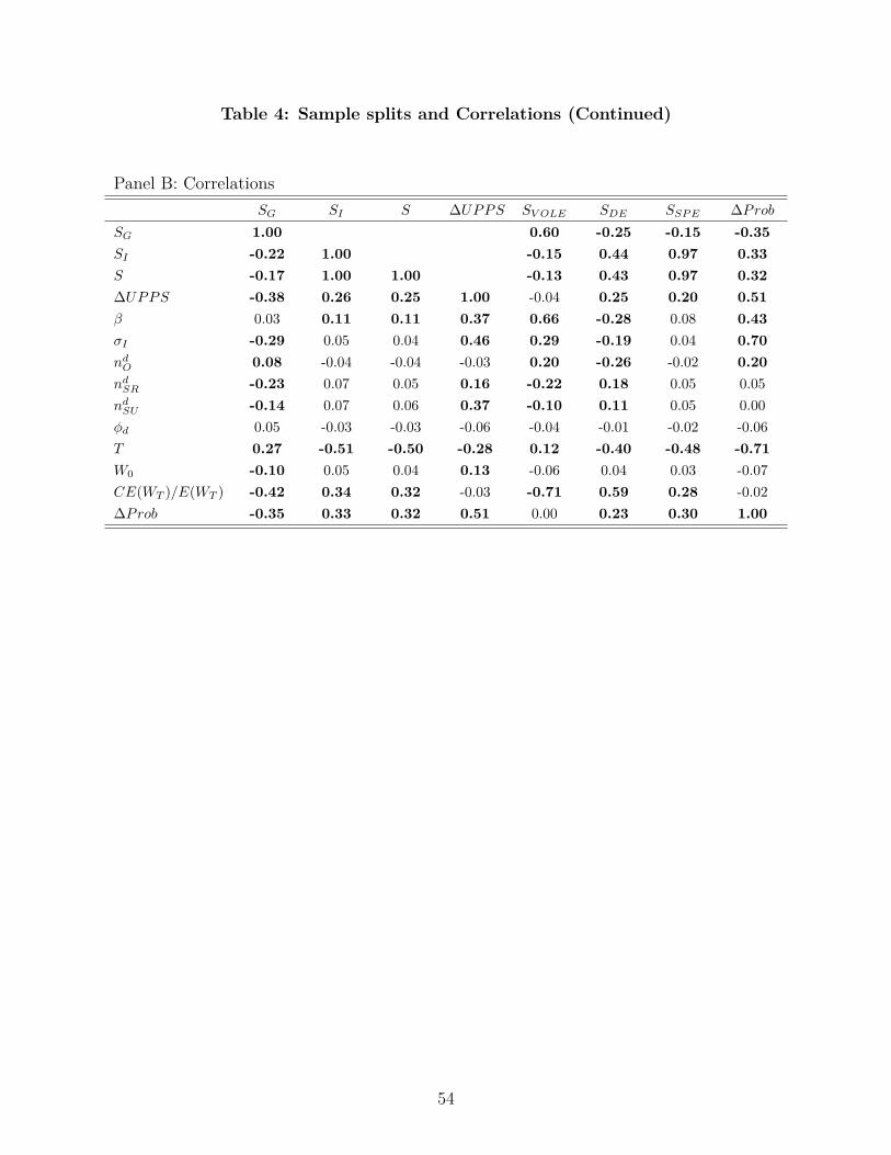
Table 4: Sample splits and Correlations (Continued)

Panel B: CorrelationsSG SI S ∆UPPS SV OLE SDE SSP E ∆Prob

SG 1.00 0.60 -0.25 -0.15 -0.35SI -0.22 1.00 -0.15 0.44 0.97 0.33S -0.17 1.00 1.00 -0.13 0.43 0.97 0.32∆UPPS -0.38 0.26 0.25 1.00 -0.04 0.25 0.20 0.51β 0.03 0.11 0.11 0.37 0.66 -0.28 0.08 0.43σI -0.29 0.05 0.04 0.46 0.29 -0.19 0.04 0.70nd

O 0.08 -0.04 -0.04 -0.03 0.20 -0.26 -0.02 0.20nd

SR -0.23 0.07 0.05 0.16 -0.22 0.18 0.05 0.05nd

SU -0.14 0.07 0.06 0.37 -0.10 0.11 0.05 0.00φd 0.05 -0.03 -0.03 -0.06 -0.04 -0.01 -0.02 -0.06T 0.27 -0.51 -0.50 -0.28 0.12 -0.40 -0.48 -0.71W0 -0.10 0.05 0.04 0.13 -0.06 0.04 0.03 -0.07CE(WT )/E(WT ) -0.42 0.34 0.32 -0.03 -0.71 0.59 0.28 -0.02∆Prob -0.35 0.33 0.32 0.51 0.00 0.23 0.30 1.00

54

Table 5: Optimal indexationThis table presents results for the case in which the firm chooses the degree of indexation ofoptions, ψ, fixed salary φ, and number of options nO. Panel A shows our results for γ = 1,Panel B for γ = 2, and Panel C for γ = 3. Each panel shows the mean of the parametersacross CEOs for five different values of the CEO’s investment in the market portfolio ω. Forthe degree of indexation ψ, the median is also reported as well as the proportion of CEOs forwhom ψ = 0 and ψ = 1 at the optimum, respectively. The table also shows the average andmedian efficiency gains from indexing expressed as a percentage of the value of the CEO’sobserved contract. Base salary is given in million dollars. All other variables except γ arepercentages.

Panel A: Results for γ = 1Mean Median

γ ω φ nO ψ = 0 ψ = 1 ψ S ψ S N1 0 1.642 1.505 92.29 1.06 3.10 0.30 0.00 0.00 7521 25 1.549 1.503 91.60 0.93 3.31 0.24 0.00 0.00 7501 50 1.596 1.499 90.58 0.93 3.59 0.32 0.00 0.00 7541 75 1.630 1.493 90.03 0.93 4.04 0.33 0.00 0.00 7521 100 1.704 1.482 89.24 0.93 4.55 0.36 0.00 0.00 753

Panel B: Results for γ = 2Mean Median

γ ω φ nO ψ = 0 ψ = 1 ψ S ψ S N2 0 1.723 1.477 82.69 1.86 8.84 1.48 0.00 0.00 7512 25 1.762 1.480 80.35 2.52 10.54 1.82 0.00 0.00 7532 50 1.793 1.479 76.46 2.93 12.74 2.28 0.00 0.00 7522 75 1.871 1.481 70.48 4.26 16.46 2.77 0.00 0.00 7522 100 1.932 1.479 64.14 8.50 22.12 3.63 0.00 0.00 753

Panel C: Results for γ = 3Mean Median

γ ω φ nO ψ = 0 ψ = 1 ψ S ψ S N3 0 1.732 1.440 76.00 3.60 13.01 3.75 0.00 0.00 7503 25 1.751 1.430 68.97 4.66 17.10 4.84 0.00 0.00 7513 50 1.834 1.411 61.87 8.53 23.46 6.07 0.00 0.00 7503 75 1.830 1.394 52.99 15.01 31.97 7.98 0.00 0.00 7533 100 1.790 1.365 45.20 25.20 41.07 10.54 25.99 0.48 750

55

Table 6: Options on indexed stockThis table repeats the analysis in Table 5 for options on indexed stock. The firm chooses thefraction ψ of conventional options to be replaced by options on indexed stock, fixed salaryφ, and number of options nO to minimize compensation cost as in Table 5. The analysis isshown for ω between 0 and 1 and γ = 2.

Mean Medianγ ω φ nO ψ = 0 ψ = 1 ψ S ψ S N2 0.00 1.859 1.390 61.30 6.65 19.30 5.48 0.00 0.00 7522 0.25 1.879 1.375 54.91 7.43 22.72 6.46 0.00 0.00 7542 0.50 1.911 1.349 47.61 8.36 27.37 7.61 8.45 0.08 7542 0.75 1.975 1.330 39.31 11.29 34.24 9.05 25.00 1.00 7532 1.00 1.937 1.290 32.45 16.36 42.73 11.08 41.03 2.60 752

Table 7: Rent extraction.This table shows results for the rent extraction case. In this case, the firm optimizes onlysubject to the incentive compatibility constraint. Panel A reports results for the full index-ation case, i.e. ψ = 1. Panel B presents results for the optimal indexation case ψ ∈ [0, 1].All results are for γ = 2.

Panel A: Results for Full Indexation (ψ = 1)Mean Median

γ ω φ nO ψ S ψ S S > 0 N2 0 1,627 2.627 100.00 -23.64 100.00 -0.58 41.14 7392 25 1,624 2.414 100.00 -18.86 100.00 -0.34 42.99 7422 50 1,622 2.420 100.00 -23.24 100.00 0.00 45.95 7402 75 1,618 2.438 100.00 -17.74 100.00 0.00 49.39 7412 100 1,617 2.282 100.00 -9.86 100.00 0.40 52.16 740

Panel B: Results for Optimal Degrees of IndexationMean Median

γ ω φ nO ψ S ψ S S > 0 N2 0 1,617 1.511 42.39 8.03 14.91 0.05 60.21 7542 25 1,616 1.516 44.38 7.68 25.48 0.20 63.18 7552 50 1,616 1.514 46.48 7.82 32.78 0.47 61.19 7552 75 1,616 1.514 49.02 8.25 44.17 0.72 64.67 7532 100 1,616 1.499 52.37 8.92 61.71 1.25 66.49 755

56

Table 8: Indexing restricted stockThis table shows results for the indexation of restricted stock. Firms can set fixed salaryφ (in million dollars), and the number of restricted shares nSR to minimize costs subjectto the participation and incentive compatibility constraints. Panel A reports results forthe full indexation case, i.e. ψ = 1. Panel B presents results for the optimal indexationcase ψ ∈ [0, 1]. All results are for γ = 2. Panel C reports rescaled savings (efficiencygains). SSR/ndSRP0 represents the efficiency gains from indexing restricted stock, expressedas a percentage of the total value of restricted stock in the observed contract. SO/n

dOBS

represents the efficiency gains from indexing options from Tables 2 and 5, expressed as apercentage of the total value of options in the observed contract.

Panel A: Results for Full Indexation (ψ = 1)Mean Median

γ ω φ nSR ψ S ψ S S > 0 N2 0 1,941 0.124 100.00 -0.63 100.00 0.00 17.35 7552 25 1,888 0.121 100.00 -0.14 100.00 0.00 20.03 7542 50 1,845 0.118 100.00 0.24 100.00 0.00 25.43 7552 75 1,806 0.115 100.00 0.52 100.00 0.00 30.46 7552 100 1,766 0.112 100.00 0.91 100.00 0.00 36.21 754

Panel B: Results for Optimal Degrees of IndexationMean Median

γ ω φ nSR ψ S ψ S S > 0 N2 0 1,804 0.121 16.89 0.44 0.00 0.00 19.60 7552 25 1,805 0.117 19.73 0.63 0.00 0.00 22.94 7542 50 1,800 0.115 24.52 0.76 0.00 0.00 27.68 7552 75 1,786 0.113 29.92 0.87 0.00 0.00 33.51 7552 100 1,762 0.111 35.44 1.14 0.00 0.00 38.41 755

Panel C: Indexing Options Compared to Indexing Restricted StockFull Indexation Optimal Indexation

γ ω SO/(nd

OBS)

SSR/(nd

SRP0)

SO/(nd

OBS)

SSR/(nd

SRP0)

2 0 -99.17 -1.63 1.78 2.212 25 -91.01 1.15 2.16 2.762 50 -70.66 3.73 2.64 3.442 75 -62.75 6.35 3.32 4.382 100 -57.43 9.23 4.31 5.62

57

Table 9: Optimal investment in the stock marketThis table repeats the analysis in Table 5 when the fraction of outside wealth invested inthe market is not restricted to be the same across CEOs. In a first step, the CEO choosesthe investment in the stock market ω ∈ [0, 1] that maximizes her utility under the observedcontract. This “quasi-optimal” investment level ω∗ is used in a second step, in which thefirm chooses the degree of indexation of options, ψ, fixed salary φ, and number of optionsnO to minimize compensation costs as in Table 5. Finally, we compute the 2nd-stage “quasi-optimal” investment level ω∗∗, which is the utility maximizing stock market investmentgiven the optimal contract from the first stage. The table shows the average ω∗, ω∗∗, andthe resulting optimal contract parameters and savings for γ = 1, 2, 3.

Mean Medianγ ω∗ ω∗∗ φ nO ψ = 0 ψ = 1 ψ S ψ S N1 0.98 0.99 1.698 1.482 89.24 0.93 4.30 0.32 0.00 0.00 7532 0.72 0.75 1.786 1.480 65.07 3.05 12.96 1.90 0.00 0.00 7533 0.42 0.44 1.800 1.436 65.07 5.20 18.36 4.41 0.00 0.00 750

Table 10: Zero market risk premiumThis table replicates results from Table 5 when the market risk premium is set to zero.Before running the main optimization, base salary φd is adjusted so that expected utilityof the contract to the executive with a market risk premium of 4% (our baseline) case isequal to the expected utility with zero market risk premium. Panel A reports results for thefull indexation case, i.e. ψ = 1. Panel B presents results for the optimal indexation caseψ ∈ [0, 1]. All results are for γ = 2.

Panel A: Results for Full Indexation (ψ = 1)Mean Median

γ ω φ nO ψ S ψ S S > 0 N2 0 18,160 2.247 100.00 -10.98 100.00 0.40 52.63 7412 25 22,798 2.275 100.00 -13.33 100.00 1.31 59.38 7462 50 26,785 2.201 100.00 -7.64 100.00 2.17 63.76 7452 75 30,180 2.048 100.00 -3.34 100.00 2.85 66.85 7452 100 32,790 2.000 100.00 -3.45 100.00 3.33 69.71 746

Panel B: Results for Optimal Degrees of IndexationMean Median

γ ω φ nO ψ S ψ S S > 0 N2 0 17,590 1.464 52.90 6.27 66.23 1.21 70.57 7412 25 22,384 1.454 59.01 7.06 85.10 1.87 73.47 7462 50 26,347 1.435 63.49 7.80 99.98 2.47 76.06 7452 75 29,728 1.406 66.57 8.54 100.00 2.97 77.53 7452 100 32,383 1.383 69.33 9.37 100.00 3.59 77.79 746

58