Indexing and Mining a Billion Time series using iSAX 2.0
31
iSAX 2.0 INDEXING & MINING ONE BILLION TIME SERIES Paper By: Alessandro Camerra Themis Palpanas Jin Shieh Eamonn Keogh
-
Upload
vasu-jain -
Category
Technology
-
view
1.736 -
download
3
Transcript of Indexing and Mining a Billion Time series using iSAX 2.0

iSAX 2.0 INDEXING & MINING
ONE BILLION TIME SERIES
Paper By:
Alessandro Camerra
Themis Palpanas
Jin Shieh
Eamonn Keogh

iSAX 2.0 INDEXING & MINING
ONE BILLION TIME SERIES
Presented by:
Vasu Jain

CONTENTS | 2
Contents
1. Introduction
2. Preliminaries
a. The SAX Representation
b. The iSAX Representation
c. Indexing iSAX
3. iSAX 2 Index
a. Bulk Loading
b. Node Splitting Policy
4. Experimental Evaluations
5. Conclusion & Future work
6. References
INTRODUCTION | 3
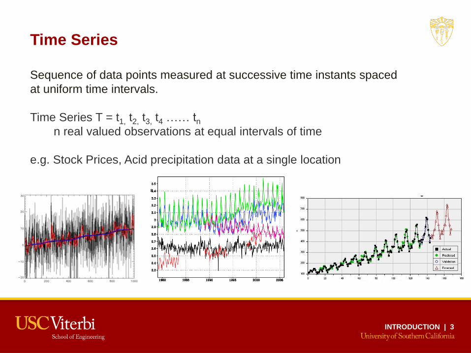
Time Series
Sequence of data points measured at successive time instants spaced
at uniform time intervals.
Time Series T = t1, t2, t3, t4 …… tn
n real valued observations at equal intervals of time
e.g. Stock Prices, Acid precipitation data at a single location
INTRODUCTION | 4
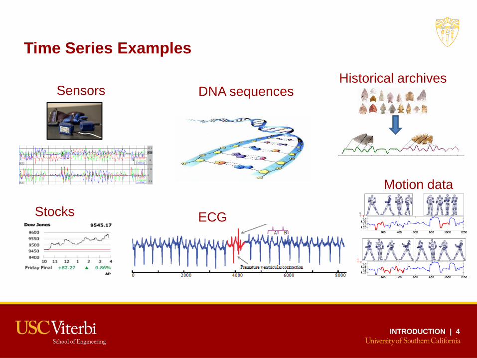
Time Series Examples
Sensors
ECG
Motion data
Stocks
data
DNA sequencesHistorical archives

INTRODUCTION | 5
Introduction
• Indexing and Mining time series is hot. There is a pressing need for
indexing and mining Time series data
• Time series of order 100 of Millions to Billions
“…we have about a million samples per minute coming in from 1000 gas turbines around the world… we need to be able to do similarity search for...” Lane Desborough, GE.“…an archival rate of 3.6 billion points a day, how can we (do similarity
search) in this data?” Josh Patterson, TVA.
• Two bottlenecks while mining these massive Time Series
• Time complexity of building the index
(6 days to index 100 million objects)
• Time to retrieve data from the disk

INTRODUCTION | 6
Introduction
• iSAX 2.0
• To solve these problem
• A data structure which is an extension to iSAX
• Suitable for indexing and mining very large time series.
• Novel mechanism for scalable indexing of time series: Bulk loading
algorithm, node splitting policies.
• Results:
• Index building time reduced by 72% with bulk loading scheme
• Index size reduced by 27%
• Number of disk page accesses reduced by 50%
• Scalability achieved allows to consider new challenges in data
mining problems which have been untenable otherwise.
• First approach that is experimentally validated to scale Time series
data collections with up to 1 Billion objects.

PRELIMINARIES | 7
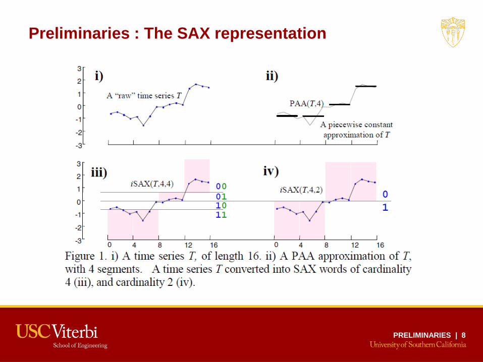
Preliminaries : The SAX representation
1. Represent a time series T of length n in w-dimensional space using PAA
Where the ith element is:
2. Then discretize into a vector of symbols
Breakpoints map to a small alphabet a of symbols
For every segment a bit wise representation is assigned to code that region
i) A time series T, of length 16. ii) A PAA approximation of T, with 4 segments.
iii) A time series T converted into SAX words of cardinality 4
-3
-2
-1
0
1
2
3
4 8 12 160
00
01
10
11
iSAX(T,4,4)
-3
-2
-1
0
1
2
3
4 8 12 160 4 8 12 160
A time series T PAA(T,4)
-3
-2
-1
0
1
2
3
i
ij
jn
wi
wn
wn
Tt1)1(
PRELIMINARIES | 8
Preliminaries : The SAX representation

PRELIMINARIES | 9
Preliminaries : The SAX representation
More About SAX Representation
1. The SAX Representation supports arbitrary breakpoints.
2. A SAX word is simply a vector of discrete numbers.
e.g. SAX word can be written as {3, 3, 1, 0} or in binary as {11, 11, 01, 00}.
3. Denoted by T4, produced by function SAX(T,4,4).
4. SAX(T, w, c) = TC where w = word length, c = cardinality of symbols
SAX(T,4,2) = T2 = {1, 1, 0, 0}SAX(T,4,4) = T2 = {11, 11, 01, 00}
5. Converting to a reduced cardinality SAX word by ignoring Trailing Bits

PRELIMINARIES | 10
Preliminaries : iSAX representation
1. Tedious to write binary string in SAX Representation
2. To include cardinality in iSAX representation we add cardinality as subscript
iSAX(T,4,8) = T8 = {68,68,38,08}3. Key property: Ability to compare two iSAX words of different cardinalities.
4. Promote the lower cardinality representation into the cardinality of the larger
Promote S2 as
5. Obtain missing bit values by returning the one closest in SAX space to the
corresponding value in T8. Not exact but admissible value of word S.
6. We can compare iSAX words where each word has mixed cardinality
{111, 11, 101, 0} = {78,34,58,02}
PRELIMINARIES | 11
Preliminaries : Indexing iSAX
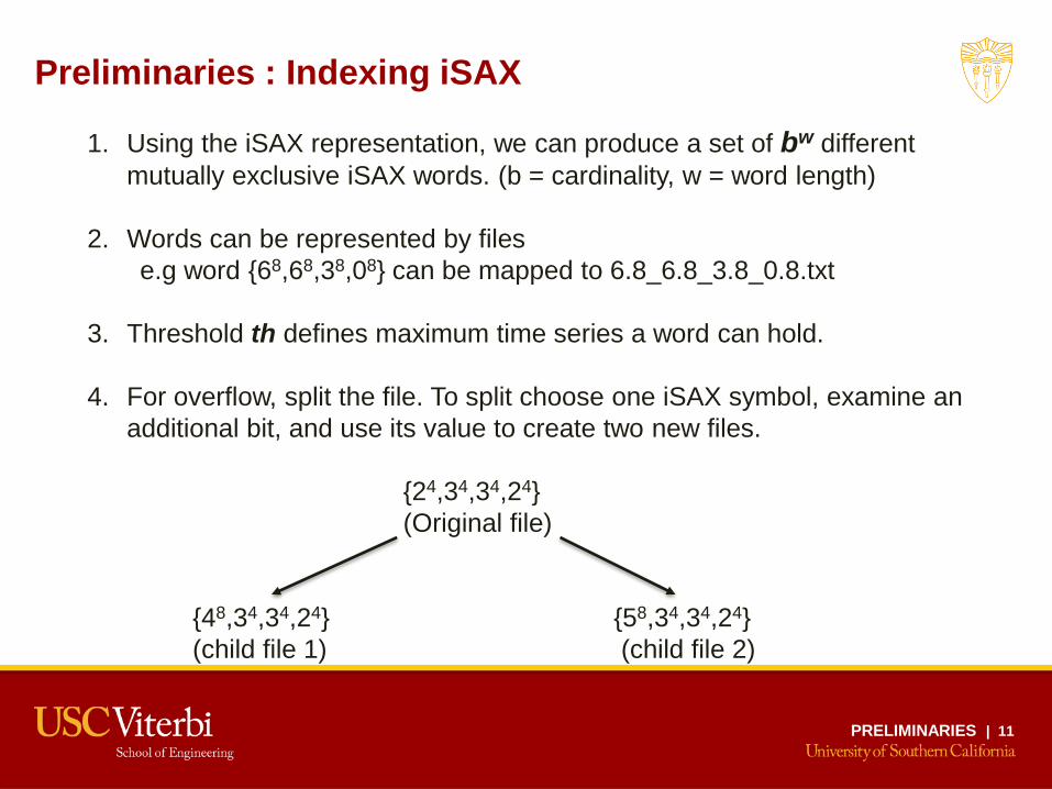
1. Using the iSAX representation, we can produce a set of bw different
mutually exclusive iSAX words. (b = cardinality, w = word length)
2. Words can be represented by files
e.g word {68,68,38,08} can be mapped to 6.8_6.8_3.8_0.8.txt
3. Threshold th defines maximum time series a word can hold.
4. For overflow, split the file. To split choose one iSAX symbol, examine an
additional bit, and use its value to create two new files.
{24,34,34,24}
(Original file)
{48,34,34,24} {58,34,34,24}
(child file 1) (child file 2)
PRELIMINARIES | 12
Preliminaries : Indexing iSAX
1. File splitting produces hierarchical, but unbalanced, index structure that
contains non-overlapping regions
2. Three class of nodes:
1. Root Node: Representative of the complete iSAX space. Contains no
SAX representation, but only pointers to the children nodes.
2. Leaf Node: Contains a pointer to an index file on disk with the raw time
series entries. Stores the highest cardinality iSAX word for each time
series.
3. Internal Node: Created when the number of time series contained by a
leaf node exceeds threshold th.
3. iSAX employs binary splits along a single dimension

iSAX 2.0 INDEX | 13
THE iSAX 2.0 INDEX
Disadvantages of iSAX
1. Take too long to build index for large datasets.
Indexing a dataset with 500 M time series takes 20 days to complete
2. Because:
• Naïve node splitting policy leading to ineffective splits and additional
disk I/O
• No bulk loading strategy, does not use available main memory to
reduce disk I/O
3. To overcome these challenges:
• New algorithm for Time series bulk loading that reduces disk I/O
• New Node splitting policy resulting in more compact index, and hence
further reducing the I/O cost.
4. We will refer to this improved iSAX index as iSAX 2.0.

iSAX 2.0 INDEX | 14
THE iSAX 2.0 INDEX
Bulk Loading
Design Principles
• Minimize the number of disk I/O operations
• Maximize sequential disk access
• Take advantage of available Main memory
Approach for Proposed solution
• Instead of building entire index at once, build distinct sub trees of index
one at a time
Assumptions
• Limited main memory i.e. less than necessary to fit entire dataset and
index

iSAX 2.0 INDEX | 15
THE iSAX 2.0 INDEX
Bulk Loading: Algorithm basics
Uses two main memory buffer layers
First Buffer Layer (FBL) :
• Corresponds to first level of iSAX 2.0 nodes
• Cluster together the Time series that will end up in same iSAX 2.0 sub
tree rooted in one of the direct children of the root.
• No size restriction, grow till they occupy available main memory.
Last Buffer Layer (LBL) :
• Corresponds to leaf nodes
• Gather all Time series of leaf nodes and flush them to disk
• Same size as of leaf nodes on disk

iSAX 2.0 INDEX | 16
THE iSAX 2.0 INDEX
Bulk Loading: Algorithm Description
Algorithm operates in two phases which alternate until entire dataset is indexed
Phase 1:
• Time series is inserted in the corresponding FBL buffer until the main
memory is almost full.
• At the end of Phase 1, we have time series collected in the FBL buffers.
• Corresponding (leaf) nodes L1, L2, L3, of the index are not yet created.

iSAX 2.0 INDEX | 17
THE iSAX 2.0 INDEX
Bulk Loading: Algorithm Description
Phase 2:
• Time series contained in each FBL buffer is moved to the appropriate
LBL buffers.
• Sequentially for each FBL buffer, the algorithm reads the time series and
creates the entire sub tree (with Internal and leaf iSAX 2.0 nodes) rooted
at the node corresponding to that FBL buffer.
• By emptying the right-most FBL buffer, we create the sub tree rooted at
internal node I1. The algorithm also creates for each leaf node a
corresponding LBL buffer
• After all Time series of a FBL buffer moves to corresponding LBL buffers,
these LBL are flushed to disk making memory available for use.

iSAX 2.0 INDEX | 18
THE iSAX 2.0 INDEX
Bulk Loading: Algorithm Description
Phase 2:
• At the end of Phase 2, all the time series from the FBL buffers have
moved down the tree to the appropriate leaf nodes and LBL buffers, and
then from the LBL buffers to the disk.
• Now both FBL and LBL are empty, and we are ready for next iteration of
our algorithm going back to Phase 1.
• This process continues until the entire dataset has been indexed.

iSAX 2.0 INDEX | 19
THE iSAX 2.0 INDEX
Node Splitting Policy
Design Principles
• Keep the index as small as can
• Avoid poor utilization of leaf nodes thus reducing the length of index
• Make splits that distribute Time series equally to children nodes
Approach for Proposed solution
• Examine for each segment the distributions of the highest cardinality
symbols across the relevant time series.
• Split the segment for which the highest cardinality iSAX symbols lie on
both sides of the breakpoint
Solution
• Split segment for which breakpoint is within range μ ± 3σ and closest to μwhere σ is Standard deviation and μ is mean for the Symbol

iSAX 2.0 INDEX | 20
THE iSAX 2.0 INDEX
Node Splitting Policy
Example
• iSAX word of length (segments) four, split a node with cardinality 2 (for
all segments). Compute μ ± 3σ value for each segment
• Segment 1 lies entirely below the lowest breakpoint of cardinality 4 (i.e.,
the cardinality of the two new nodes after the split) ∴ No Split
• Segments 2 and 3 ranges cross some breakpoint of cardinality 4.
Split on segment 3, because its μ value lies closer to a breakpoint than
that of segment 2.
• This tells some of the time series in the node to be split will end up in
the new node representing the area above the breakpoint, while the rest
will move to the second new node thus, achieving a balanced split.

iSAX 2.0 INDEX | 21
THE iSAX 2.0 INDEX
Node Splitting Policy
iSAX 2.0 INDEX | 22
THE iSAX 2.0 INDEX
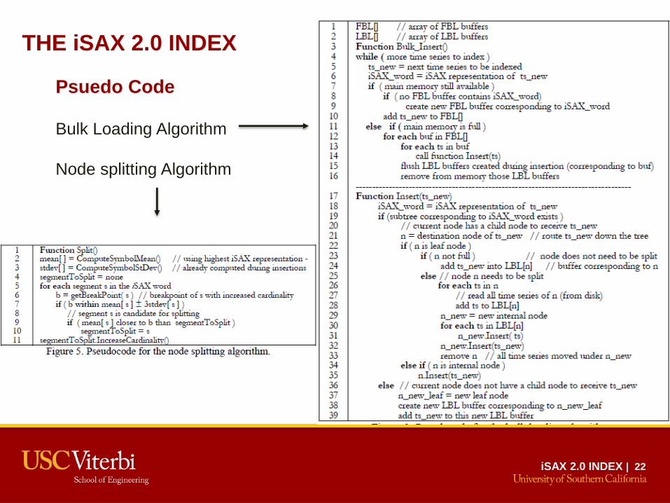
Psuedo Code
Bulk Loading Algorithm
Node splitting Algorithm
EXPERIMENTAL EVALUATION | 23
Experimental Evaluation
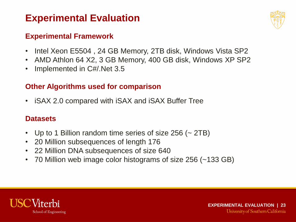
Experimental Framework
• Intel Xeon E5504 , 24 GB Memory, 2TB disk, Windows Vista SP2
• AMD Athlon 64 X2, 3 GB Memory, 400 GB disk, Windows XP SP2
• Implemented in C#/.Net 3.5
Other Algorithms used for comparison
• iSAX 2.0 compared with iSAX and iSAX Buffer Tree
Datasets
• Up to 1 Billion random time series of size 256 (~ 2TB)
• 20 Million subsequences of length 176
• 22 Million DNA subsequences of size 640
• 70 Million web image color histograms of size 256 (~133 GB)
EXPERIMENTAL EVALUATION | 24
Experimental Evaluation
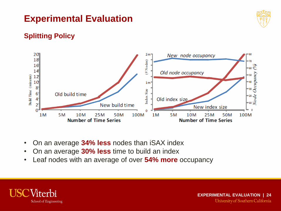
Splitting Policy
• On an average 34% less nodes than iSAX index
• On an average 30% less time to build an index
• Leaf nodes with an average of over 54% more occupancy
EXPERIMENTAL EVALUATION | 25
Experimental Evaluation
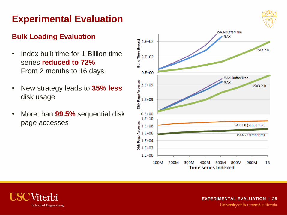
Bulk Loading Evaluation
• Index built time for 1 Billion time
series reduced to 72%
From 2 months to 16 days
• New strategy leads to 35% less
disk usage
• More than 99.5% sequential disk
page accesses
EXPERIMENTAL EVALUATION | 26
Experimental Evaluation
Case Study in Entomology
• Early detection of harmful insect behavior
• 20 Million Time series of size 176
• 6 Hours to index (~ 27 GB disk space), 0.5 second to answer 1-NN query
Mining Massive DNA Sequences
• Investigating genetic relationships
• 22 Million Time series of size 640
• 9 Hours to index (~ 115 GB disk space), 0.6 second to answer 10-NN query
Mining Massive Image collections
• Finding similar images
• 70 Million web image color histograms of size 256 (~133 GB)
• 12 Hours to index (~ 133 GB disk space), 0.9 second to answer 1-NN query
EXPERIMENTAL EVALUATION | 27
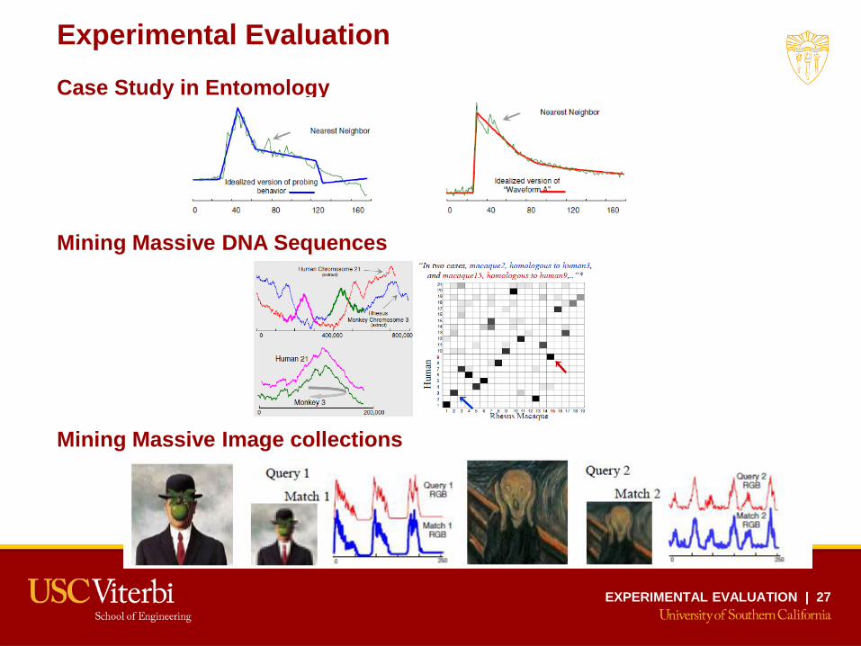
Experimental Evaluation
Case Study in Entomology
Mining Massive DNA Sequences
Mining Massive Image collections

CONCLUSIONS & FUTURE WORK | 28
Conclusions and future work
Conclusions
Proposed iSAX 2.0
• indexing for billion size time series collections
Experimentally validated proposed approach
• First published experiment with analysis over 1 Billion time series
Case studies in diverse domains shows usefulness of this approach
• Analysis of vast collection of data in fields like Etymology, web
mining, DNA sequencing etc.
Future Work
Index and mine larger time series of order 10 Billion or more
• e.g. Functional magnetic resonance imaging (fMRI)
• Single experiment (1 subject, 1 test) produces 60,000 TS of length
3000 leading to 12GB

REFERENCES | 29
REFERENCES
• iSAX 2.0 Indexing and Mining Billion time Series : Alessandro Camerra, Themis
Palpanas, Jin Shieh and Eamonn Keogh (2010) ICDM 2010 [pdf]
• Microsoft Research iSAX 2.0: Indexing and Mining One Billion Time Series
MSR URL
• Images Source 1, Source 2

REFERENCES | 29
THANK YOU
Q / A