Indexing and Hashing - CAS – Central Authentication...
123
©Silberschatz, Korth and Sudarshan 1 Indexing and Hashing Basic Index Concepts Ordered Indices B + -Tree Index Files Hashing Index Definition in SQL Multiple-Key Access Bitmap Indices
Transcript of Indexing and Hashing - CAS – Central Authentication...

©Silberschatz, Korth and Sudarshan1
Indexing and Hashing
Basic Index Concepts
Ordered Indices
B+-Tree Index Files
Hashing
Index Definition in SQL
Multiple-Key Access
Bitmap Indices
©Silberschatz, Korth and Sudarshan2
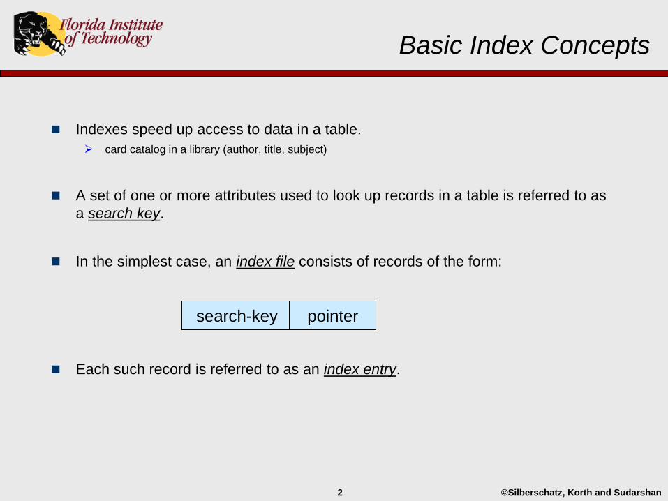
Basic Index Concepts
Indexes speed up access to data in a table.
card catalog in a library (author, title, subject)
A set of one or more attributes used to look up records in a table is referred to as
a search key.
In the simplest case, an index file consists of records of the form:
Each such record is referred to as an index entry.
search-key pointer
©Silberschatz, Korth and Sudarshan3
Basic Index Concepts, Cont.
An index file is a file, and suffers from many of the same problems as a data file,
and uses some of the same organization techniques, e.g., pointer chains.
Index files are typically much smaller than the original file.
10% - 25% is not unusual.
Two kinds of indices, primarily:
Ordered indices - entries are stored in sorted order, based on the search key.
Hash indices – entries are distributed uniformly across “buckets” using a “hash function.”
©Silberschatz, Korth and Sudarshan4
Index Evaluation Metrics
All indices are not created equal…
In an OLTP environment - Insertion, deletion and update time are important.
In a DSS environment - access time is important:
Point Queries - Records with a specified value in an attribute.
Range Queries - Records with an attribute value in a specified range.
In either case, space used is also important.

©Silberschatz, Korth and Sudarshan5
Ordered Indices
An index whose search key specifies the sequential order of the data file is a
primary index.
Also called clustering or clustered index.
Search key of a primary index is frequently the primary key.
An index whose search key does not specify the sequential order of the data file
is a secondary index.
Also called a non-clustering or non-clustered index.
A sorted data file with a primary index on it is commonly referred to as an index-
sequential file.
©Silberschatz, Korth and Sudarshan6
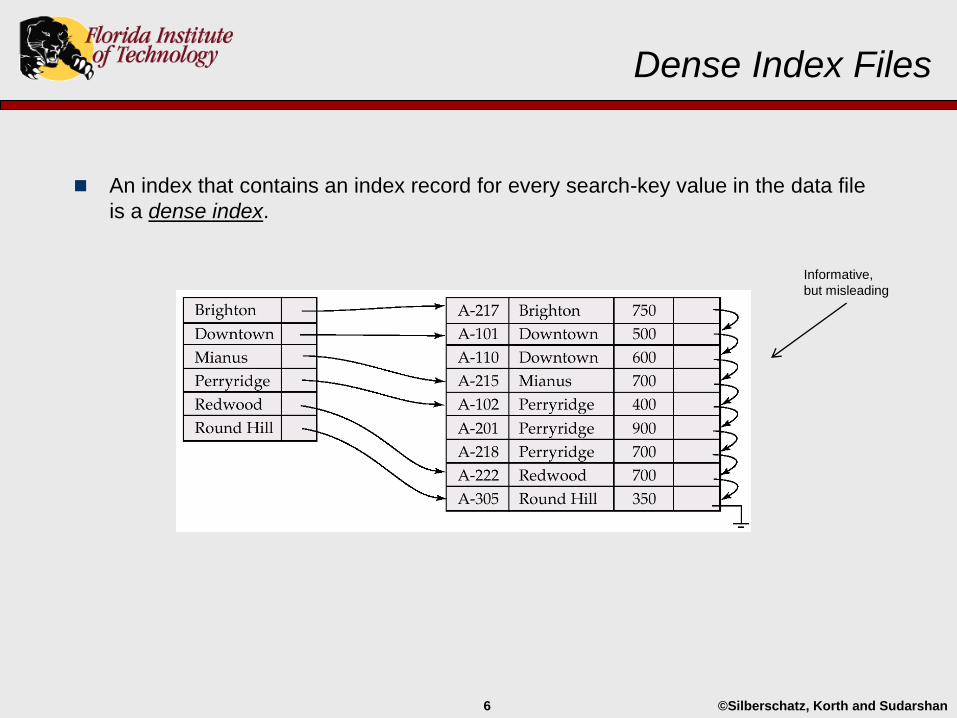
Dense Index Files
An index that contains an index record for every search-key value in the data file
is a dense index.
Informative,
but misleading
©Silberschatz, Korth and Sudarshan7
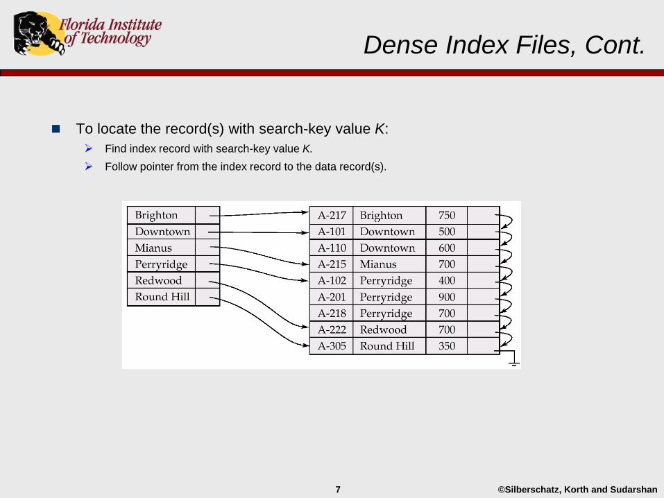
Dense Index Files, Cont.
To locate the record(s) with search-key value K:
Find index record with search-key value K.
Follow pointer from the index record to the data record(s).
©Silberschatz, Korth and Sudarshan8
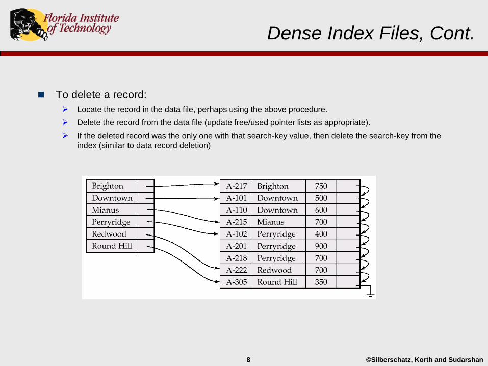
Dense Index Files, Cont.
To delete a record:
Locate the record in the data file, perhaps using the above procedure.
Delete the record from the data file (update free/used pointer lists as appropriate).
If the deleted record was the only one with that search-key value, then delete the search-key from the
index (similar to data record deletion)
©Silberschatz, Korth and Sudarshan9
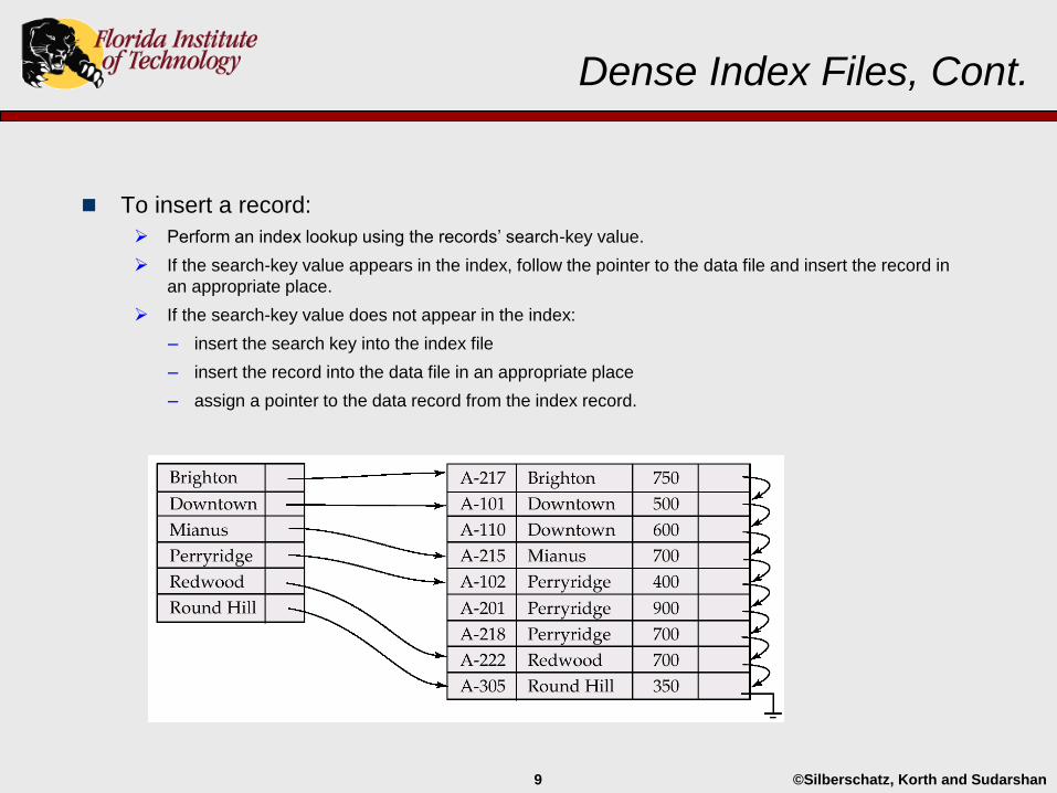
Dense Index Files, Cont.
To insert a record:
Perform an index lookup using the records’ search-key value.
If the search-key value appears in the index, follow the pointer to the data file and insert the record in
an appropriate place.
If the search-key value does not appear in the index:
– insert the search key into the index file
– insert the record into the data file in an appropriate place
– assign a pointer to the data record from the index record.

©Silberschatz, Korth and Sudarshan10
Sparse Index Files
An index that contains index records but only for some search-key values in the
data file is a sparse index.
Typically one index entry for each data file block.
©Silberschatz, Korth and Sudarshan11
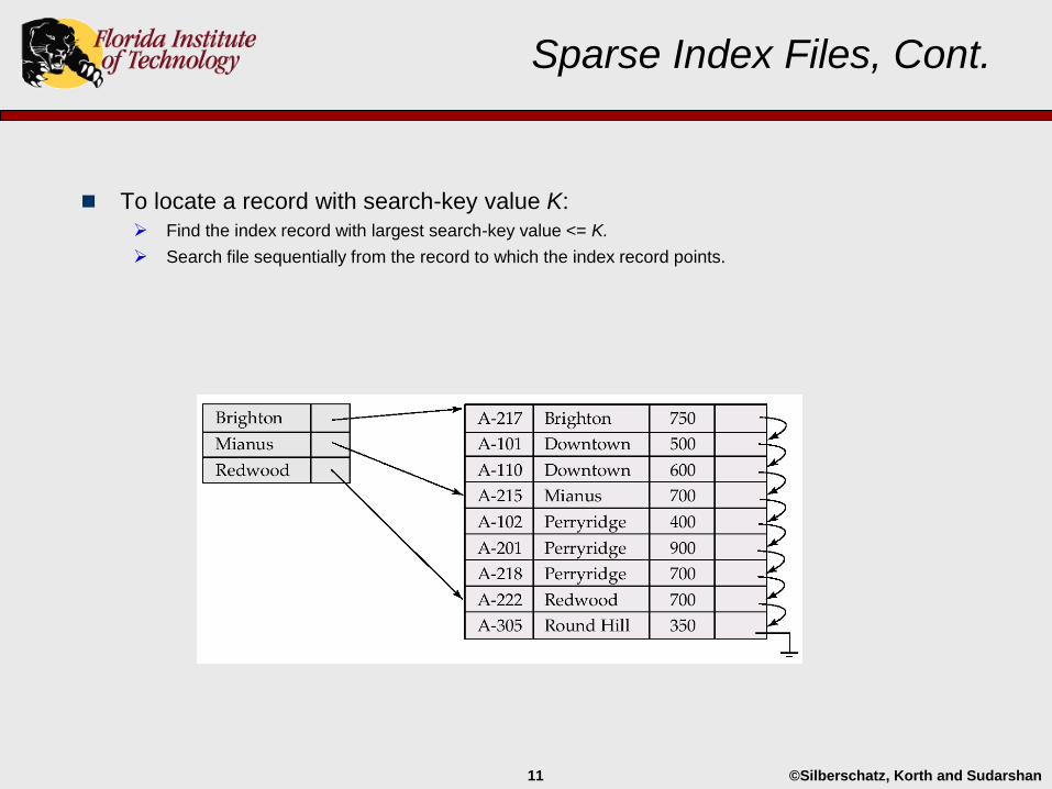
Sparse Index Files, Cont.
To locate a record with search-key value K:
Find the index record with largest search-key value <= K.
Search file sequentially from the record to which the index record points.
©Silberschatz, Korth and Sudarshan12
Sparse Index Files, Cont.
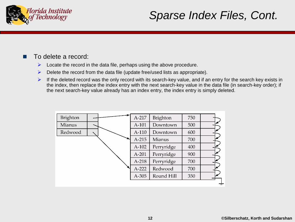
To delete a record:
Locate the record in the data file, perhaps using the above procedure.
Delete the record from the data file (update free/used lists as appropriate).
If the deleted record was the only record with its search-key value, and if an entry for the search key exists in the index, then replace the index entry with the next search-key value in the data file (in search-key order); if the next search-key value already has an index entry, the index entry is simply deleted.
©Silberschatz, Korth and Sudarshan13
Sparse Index Files, Cont.
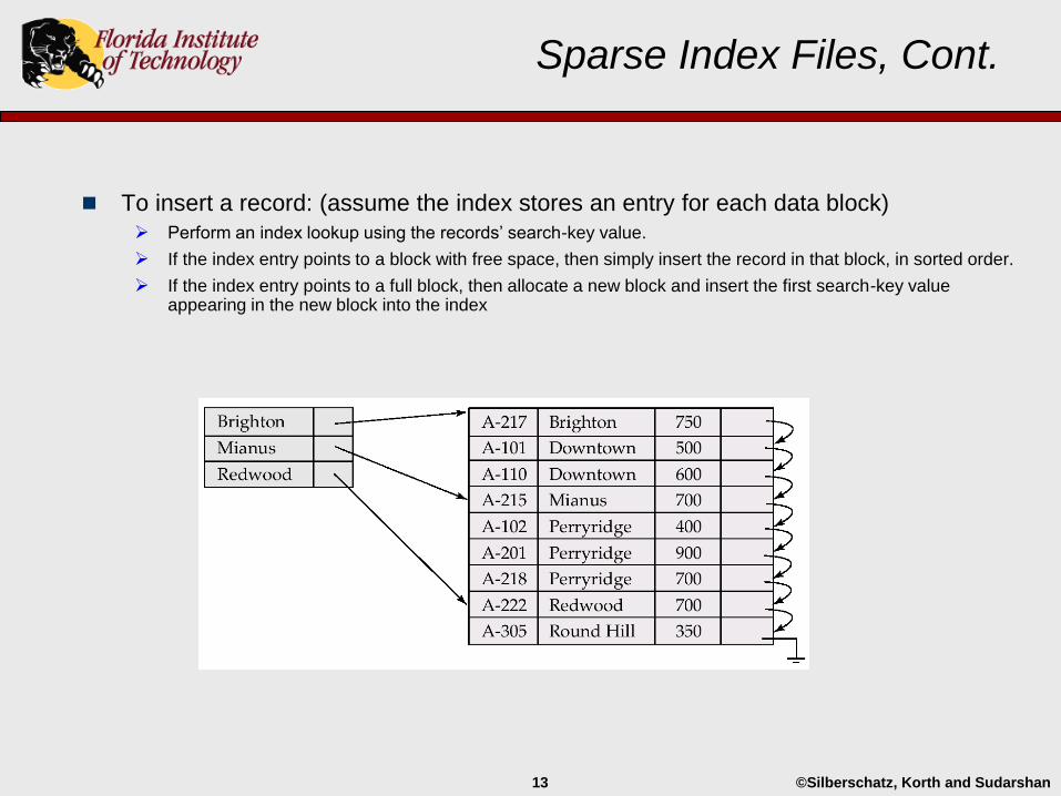
To insert a record: (assume the index stores an entry for each data block)
Perform an index lookup using the records’ search-key value.
If the index entry points to a block with free space, then simply insert the record in that block, in sorted order.
If the index entry points to a full block, then allocate a new block and insert the first search-key value appearing in the new block into the index
©Silberschatz, Korth and Sudarshan14
Sparse Index Files, Cont.
Advantages (relative to dense indices):
Require less space
Less maintenance for insertions and deletions
Disadvantages:
Slower for locating records, especially if there is more than one block per index entry
©Silberschatz, Korth and Sudarshan15
Multilevel Index
In order to improve performance, an attempt is frequently made to store, i.e., pin,
all index blocks in memory.
Unfortunately, sometimes an index is too big to fit into memory.
In such a case, the index can be treated as a sequential file on disk and a
sparse index is built on it:
outer index – a sparse index
inner index – sparse or dense index
If the outer index is still too large to fit in main memory, yet another level of index
can be created, and so on.
©Silberschatz, Korth and Sudarshan16
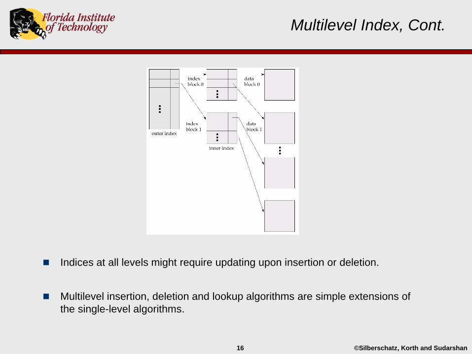
Multilevel Index, Cont.
Indices at all levels might require updating upon insertion or deletion.
Multilevel insertion, deletion and lookup algorithms are simple extensions of
the single-level algorithms.
©Silberschatz, Korth and Sudarshan17
Secondary Indices
So far, our consideration of dense and sparse indices has only been in the
context of primary indices.
Recall that an index whose search key does not specify the sequential order of
the data file is called a secondary index.
A secondary index can be helpful when a table is searched using a search key
other than the one on which the table is sorted.
Suppose account is sorted by account number, but searches are based on branch, or searching for
a range of balances.
Suppose payment is sorted by loan# and payment#, but searches are based on id#
©Silberschatz, Korth and Sudarshan18
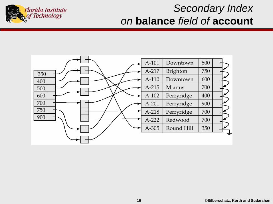
Secondary Indices
In a secondary index, each index entry will point to either a:
Single record containing the search key value (candidate key).
Bucket that contains pointers to all records with that search-key value (non-candidate key).
All previous algorithms and data structures can be modified to apply to
secondary indices.
©Silberschatz, Korth and Sudarshan19
Secondary Index
on balance field of account
©Silberschatz, Korth and Sudarshan20
Index Classification
In summary, the indices we have considered so far are either:
Dense, or
Sparse
In addition, an index may be either:
Primary, or
Secondary
And the search key the index is built on may be either a:
Candidate key
Non-candidate key
Note, that the book claims a secondary index must be dense; why?
©Silberschatz, Korth and Sudarshan21
Index Performance
Although Indices improve performance, they can also hurt:
All indices must be updated upon insertion or deletion.
Performance degrades as the index file grows (physical order doesn’t match logical order, many overflow blocks get created, etc) consequently periodic reorganization (delete and rebuild) of the index is required.
Scanning a file sequentially in secondary search-key order can be expensive; worst case - each record
access may fetch a new block from disk**
Thus, in the worst case, the number of data blocks retrieved when scanning a
secondary index for a range query is equal to the number of tuples retrieved.
©Silberschatz, Korth and Sudarshan22
B+-Tree Index Files
B+-tree indices are a type of multi-level index.
Advantage of B+-tree index files:
Automatically reorganizes itself with small, local, changes.
Index reorganization is still required, but not as frequently*.
Disadvantage of B+-trees - extra time (insertion, deletion) and space overhead.
Advantages outweigh the disadvantages, and they are used extensively – the “gold standard” of index structures.
©Silberschatz, Korth and Sudarshan23
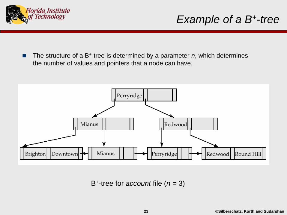
Example of a B+-tree
B+-tree for account file (n = 3)
The structure of a B+-tree is determined by a parameter n, which determines
the number of values and pointers that a node can have.
©Silberschatz, Korth and Sudarshan24
Observations about B+-trees
Each node is typically a disk block:
“logically” close blocks need not be “physically” close.
The value of n is typically determined by:
Block size
Search key size
Pointer size
i.e., we squeeze in as many search-keys and pointers as possible.
©Silberschatz, Korth and Sudarshan25
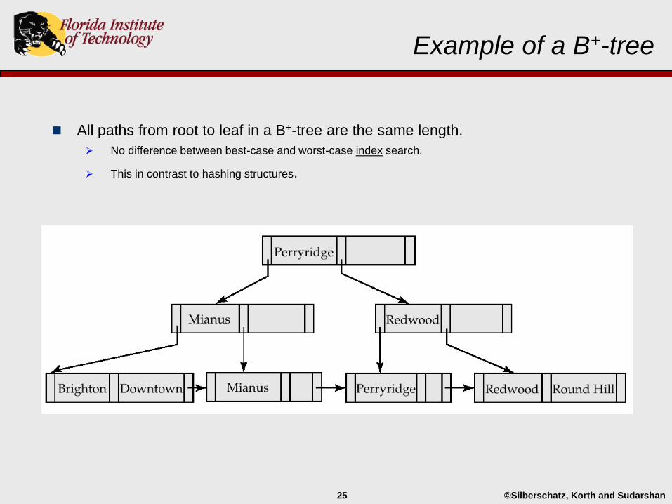
Example of a B+-tree
All paths from root to leaf in a B+-tree are the same length.
No difference between best-case and worst-case index search.
This in contrast to hashing structures.
©Silberschatz, Korth and Sudarshan26
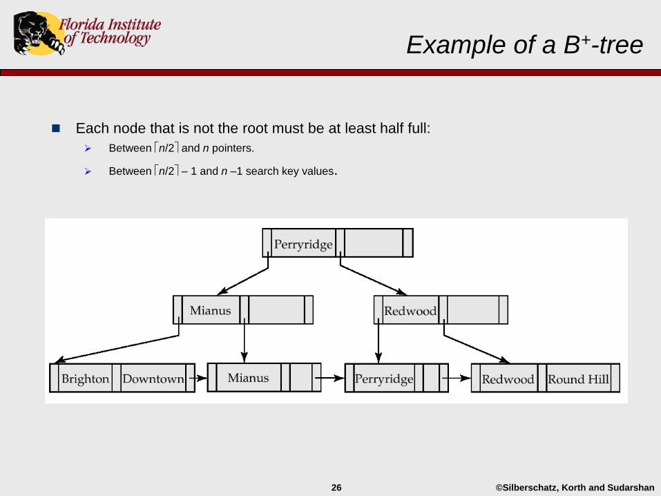
Example of a B+-tree
Each node that is not the root must be at least half full:
Between n/2 and n pointers.
Between n/2 – 1 and n –1 search key values.
©Silberschatz, Korth and Sudarshan27
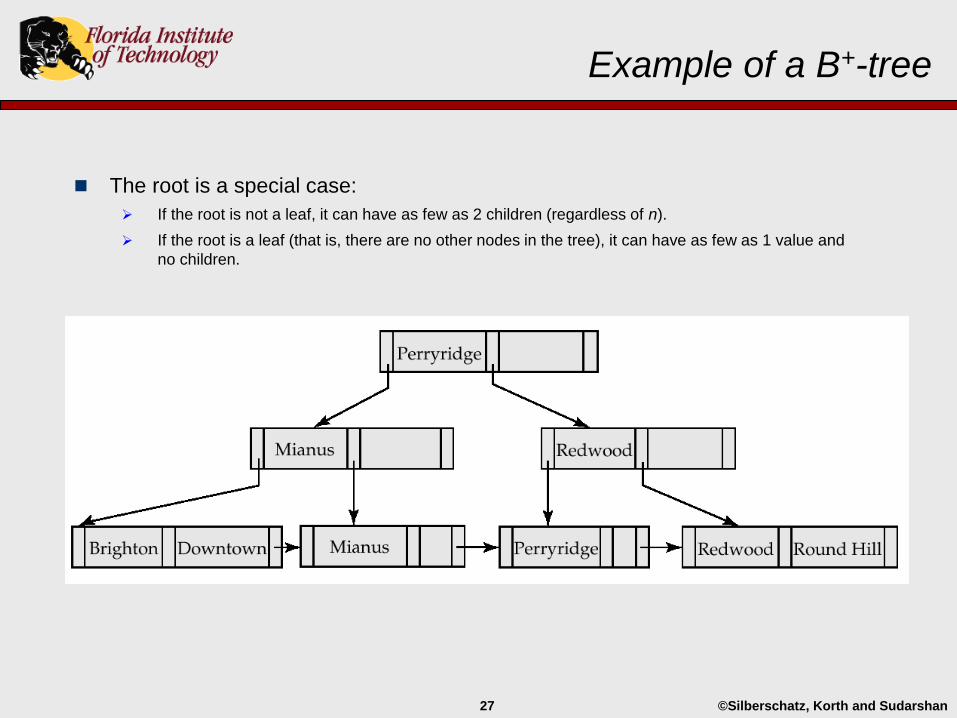
Example of a B+-tree
The root is a special case:
If the root is not a leaf, it can have as few as 2 children (regardless of n).
If the root is a leaf (that is, there are no other nodes in the tree), it can have as few as 1 value and
no children.
©Silberschatz, Korth and Sudarshan28
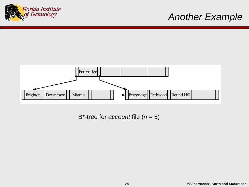
Another Example
B+-tree for account file (n = 5)
©Silberschatz, Korth and Sudarshan29
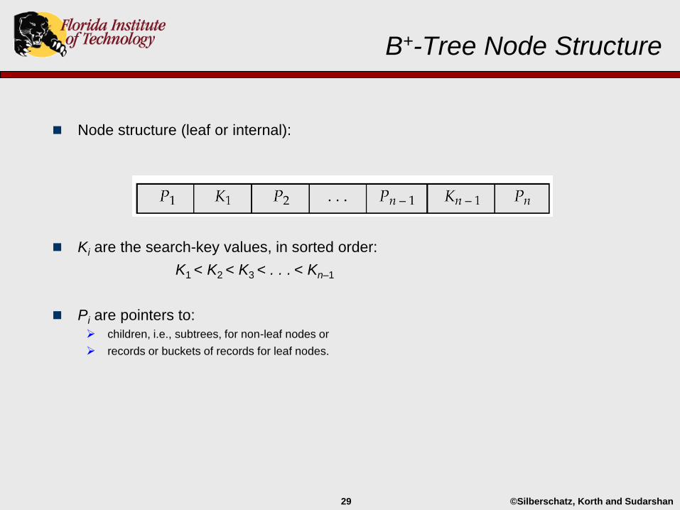
B+-Tree Node Structure
Node structure (leaf or internal):
Ki are the search-key values, in sorted order:
K1 < K2 < K3 < . . . < Kn–1
Pi are pointers to:
children, i.e., subtrees, for non-leaf nodes or
records or buckets of records for leaf nodes.
©Silberschatz, Korth and Sudarshan30
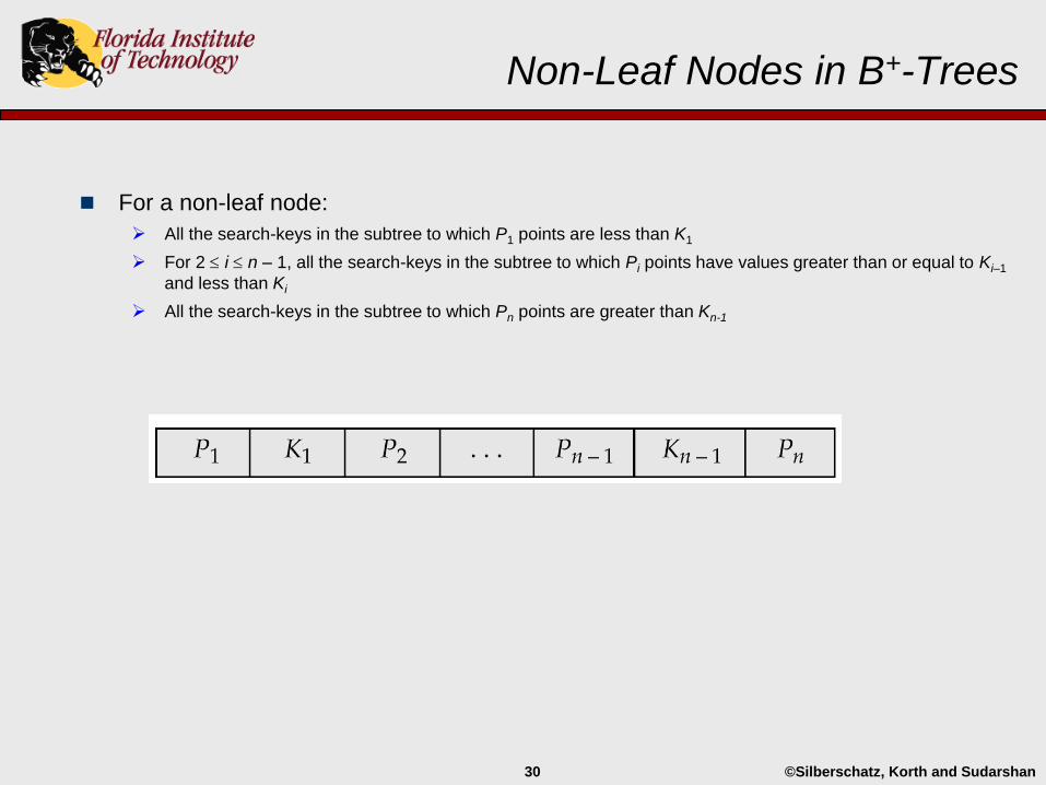
Non-Leaf Nodes in B+-Trees
For a non-leaf node:
All the search-keys in the subtree to which P1 points are less than K1
For 2 i n – 1, all the search-keys in the subtree to which Pi points have values greater than or equal to Ki–1
and less than Ki
All the search-keys in the subtree to which Pn points are greater than Kn-1
©Silberschatz, Korth and Sudarshan31
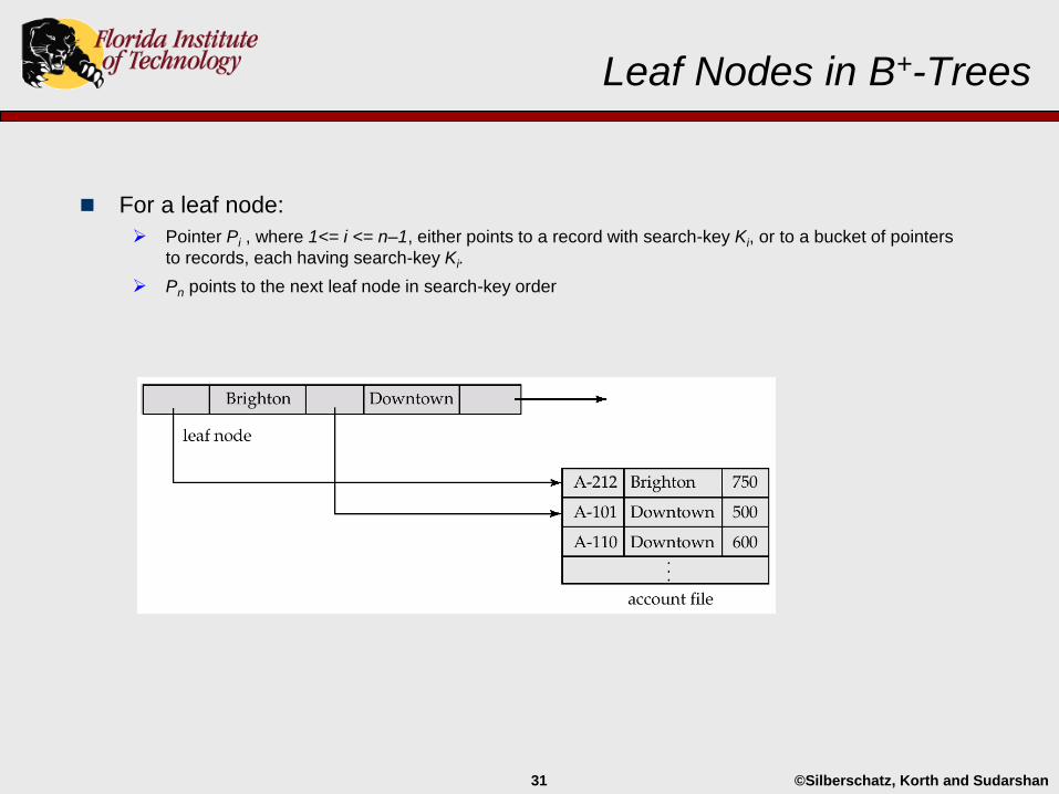
Leaf Nodes in B+-Trees
For a leaf node:
Pointer Pi , where 1<= i <= n–1, either points to a record with search-key Ki, or to a bucket of pointers
to records, each having search-key Ki.
Pn points to the next leaf node in search-key order
©Silberschatz, Korth and Sudarshan32
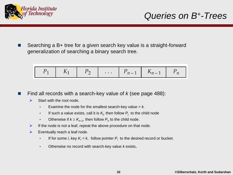
Queries on B+-Trees
Searching a B+ tree for a given search key value is a straight-forward
generalization of searching a binary search tree.
Find all records with a search-key value of k (see page 488):
Start with the root node.
• Examine the node for the smallest search-key value > k.
• If such a value exists, call it is Kj, then follow Pj to the child node
• Otherwise if k Kn–1, then follow Pn to the child node.
If the node is not a leaf, repeat the above procedure on that node.
Eventually reach a leaf node.
• If for some i, key Ki = k, follow pointer Pi to the desired record or bucket.
• Otherwise no record with search-key value k exists.
©Silberschatz, Korth and Sudarshan33
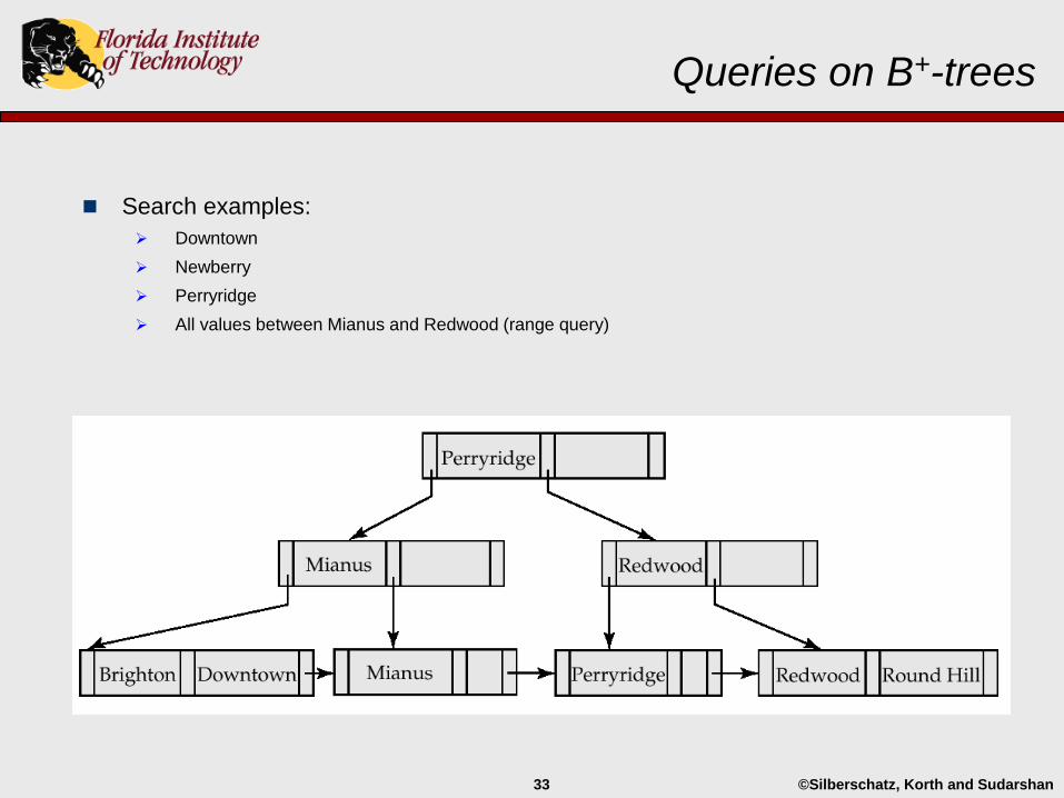
Queries on B+-trees
Search examples:
Downtown
Newberry
Perryridge
All values between Mianus and Redwood (range query)
©Silberschatz, Korth and Sudarshan34
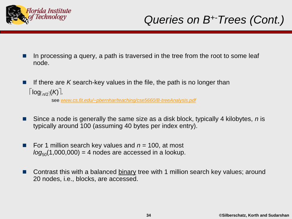
Queries on B+-Trees (Cont.)
In processing a query, a path is traversed in the tree from the root to some leaf node.
If there are K search-key values in the file, the path is no longer than
logn/2(K).
see www.cs.fit.edu/~pbernhar/teaching/cse5660/B-treeAnalysis.pdf
Since a node is generally the same size as a disk block, typically 4 kilobytes, n is typically around 100 (assuming 40 bytes per index entry).
For 1 million search key values and n = 100, at most log50(1,000,000) = 4 nodes are accessed in a lookup.
Contrast this with a balanced binary tree with 1 million search key values; around 20 nodes, i.e., blocks, are accessed.

©Silberschatz, Korth and Sudarshan35
Queries on B+-Trees (Cont.)
The authors claim (without proof or analysis) that if there are K search-key values in the file, the path is no longer than:
logn/2(K)
The analysis from the previous page shows that the path is no longer than:
2 + logd(K/e)
where d = n/2 and e = (n-1)/2.
Although the above expressions are different, both are O(logK), since d and e are fixed for any given index.
©Silberschatz, Korth and Sudarshan36
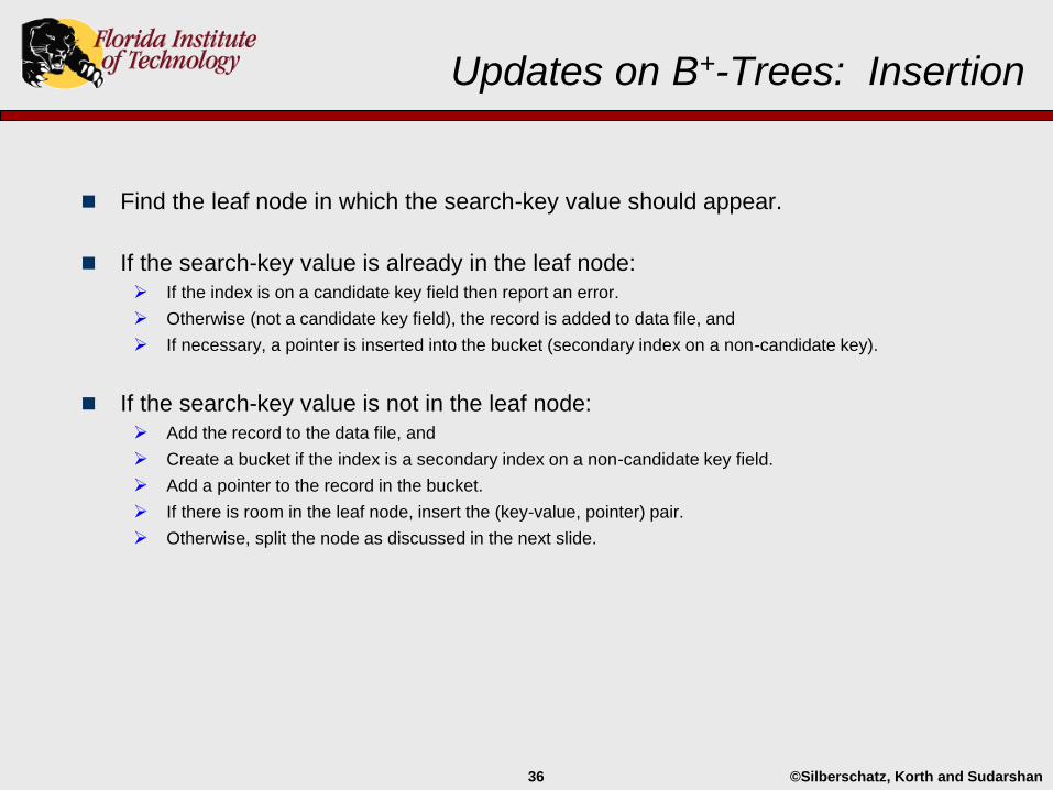
Updates on B+-Trees: Insertion
Find the leaf node in which the search-key value should appear.
If the search-key value is already in the leaf node:
If the index is on a candidate key field then report an error.
Otherwise (not a candidate key field), the record is added to data file, and
If necessary, a pointer is inserted into the bucket (secondary index on a non-candidate key).
If the search-key value is not in the leaf node:
Add the record to the data file, and
Create a bucket if the index is a secondary index on a non-candidate key field.
Add a pointer to the record in the bucket.
If there is room in the leaf node, insert the (key-value, pointer) pair.
Otherwise, split the node as discussed in the next slide.
©Silberschatz, Korth and Sudarshan37
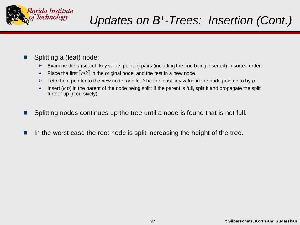
Updates on B+-Trees: Insertion (Cont.)
Splitting a (leaf) node:
Examine the n (search-key value, pointer) pairs (including the one being inserted) in sorted order.
Place the first n/2 in the original node, and the rest in a new node.
Let p be a pointer to the new node, and let k be the least key value in the node pointed to by p.
Insert (k,p) in the parent of the node being split; If the parent is full, split it and propagate the split further up (recursively).
Splitting nodes continues up the tree until a node is found that is not full.
In the worst case the root node is split increasing the height of the tree.
©Silberschatz, Korth and Sudarshan38
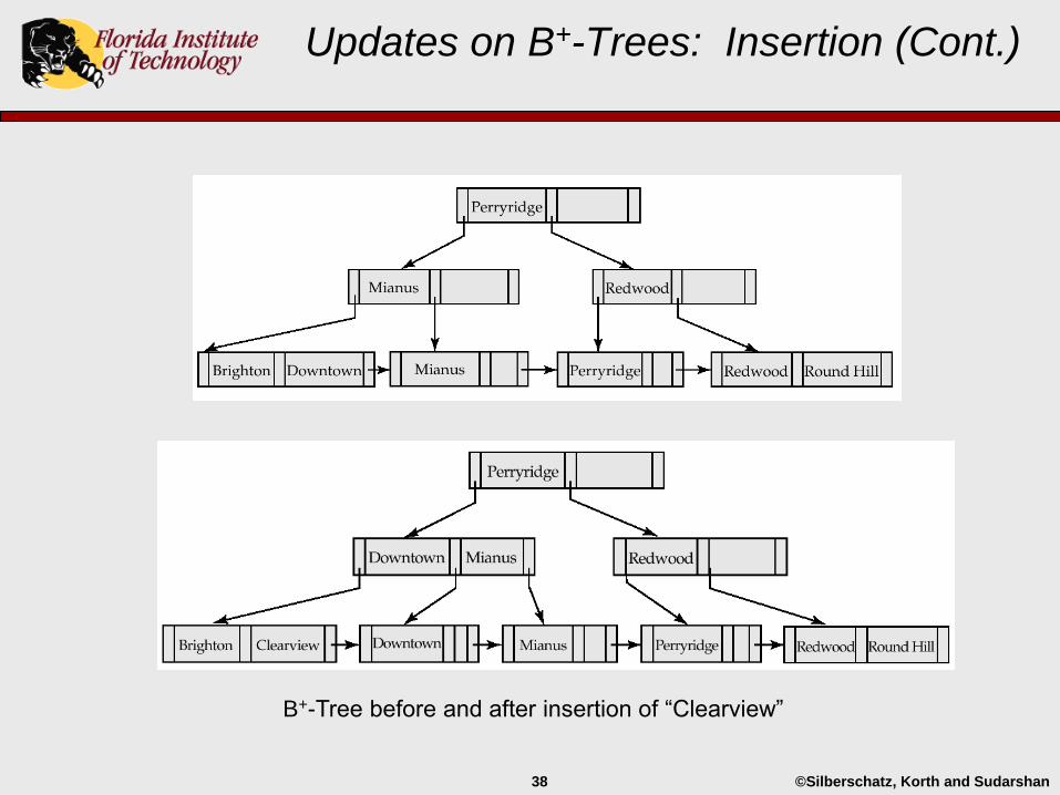
Updates on B+-Trees: Insertion (Cont.)
B+-Tree before and after insertion of “Clearview”
©Silberschatz, Korth and Sudarshan39
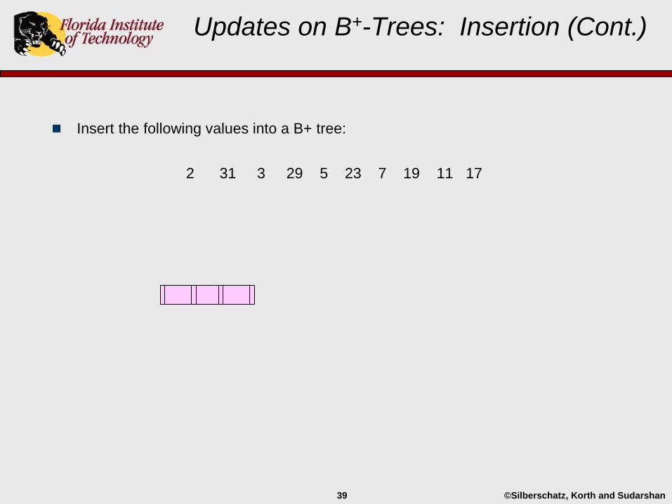
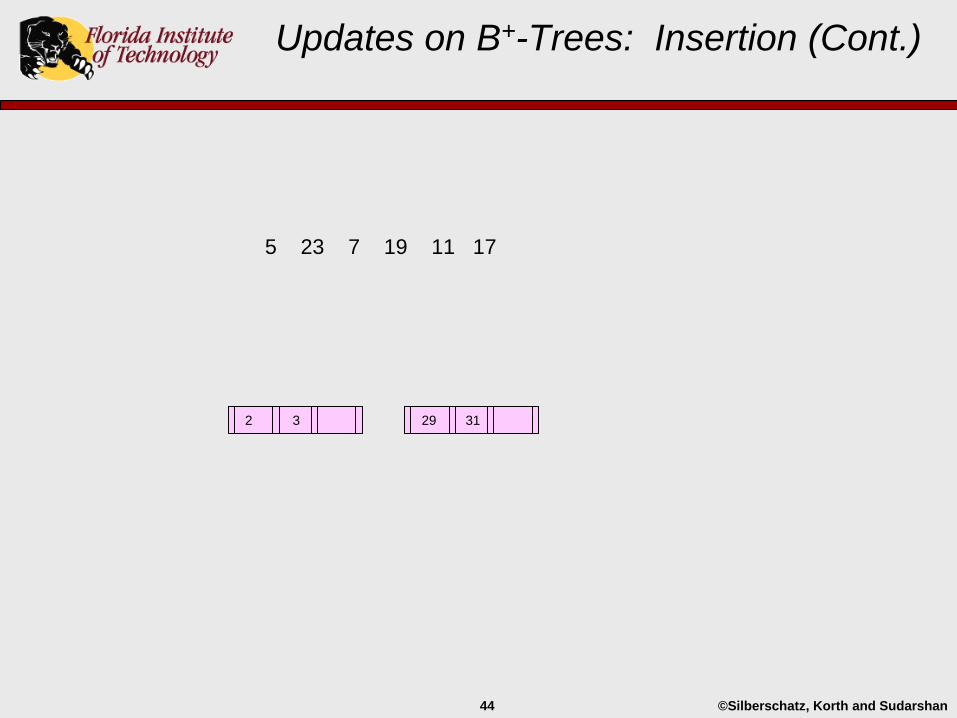
Insert the following values into a B+ tree:
2 31 3 29 5 23 7 19 11 17
Updates on B+-Trees: Insertion (Cont.)
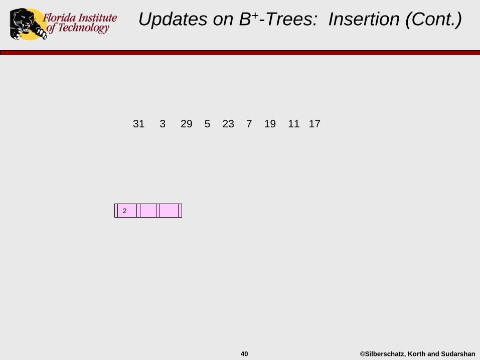
©Silberschatz, Korth and Sudarshan40
31 3 29 5 23 7 19 11 17
Updates on B+-Trees: Insertion (Cont.)
2
©Silberschatz, Korth and Sudarshan41
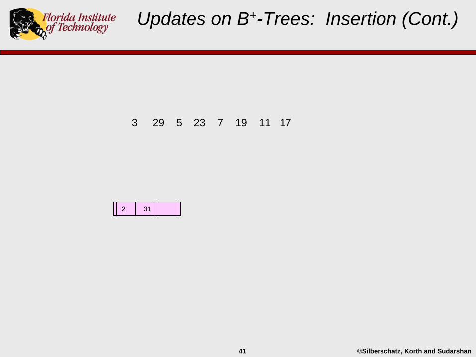
3 29 5 23 7 19 11 17
Updates on B+-Trees: Insertion (Cont.)
2 31
©Silberschatz, Korth and Sudarshan42
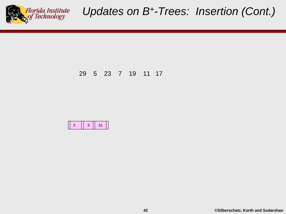
29 5 23 7 19 11 17
Updates on B+-Trees: Insertion (Cont.)
2 3 31
©Silberschatz, Korth and Sudarshan43
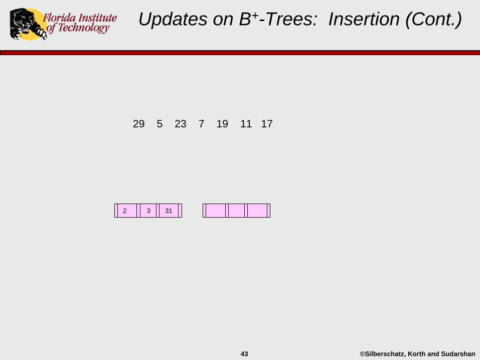
29 5 23 7 19 11 17
Updates on B+-Trees: Insertion (Cont.)
2 3 31
©Silberschatz, Korth and Sudarshan44
5 23 7 19 11 17
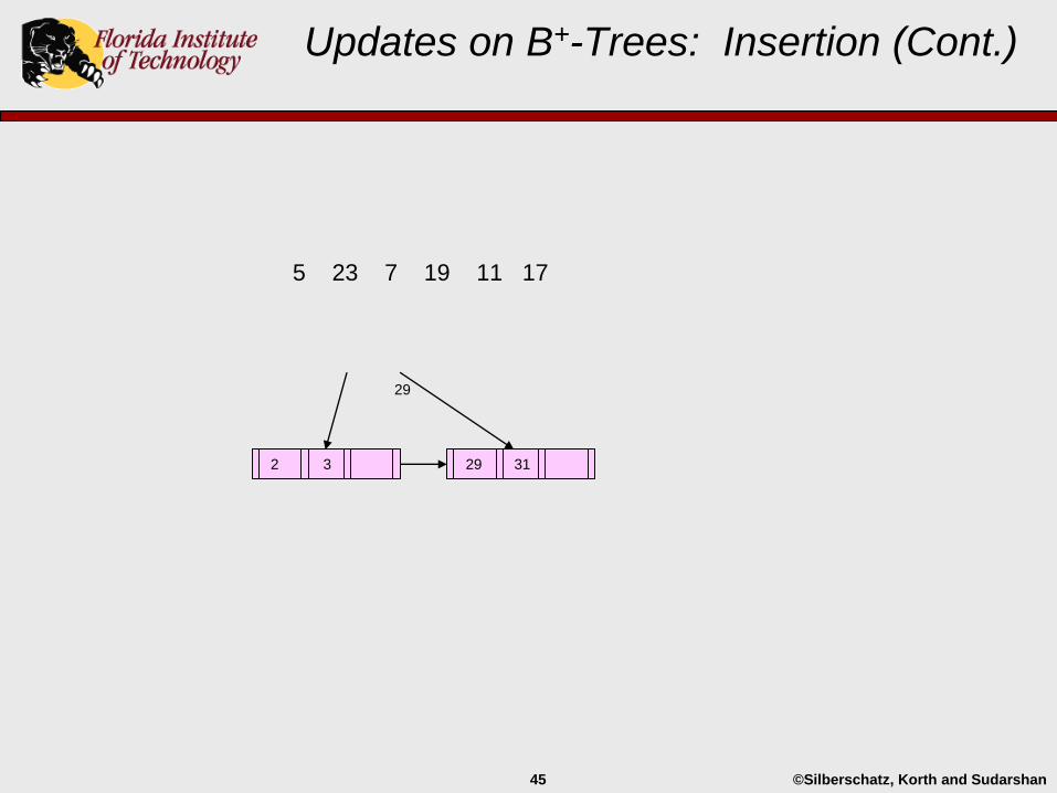
Updates on B+-Trees: Insertion (Cont.)
2 3 29 31
©Silberschatz, Korth and Sudarshan45
5 23 7 19 11 17
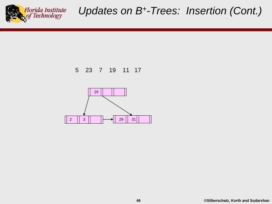
Updates on B+-Trees: Insertion (Cont.)
2 3 29 31
29
©Silberschatz, Korth and Sudarshan46
5 23 7 19 11 17
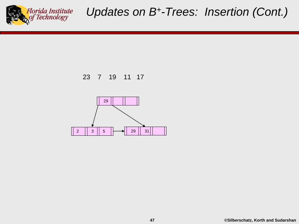
Updates on B+-Trees: Insertion (Cont.)
2 3 29 31
29
©Silberschatz, Korth and Sudarshan47
23 7 19 11 17
Updates on B+-Trees: Insertion (Cont.)
2 3 5 29 31
29
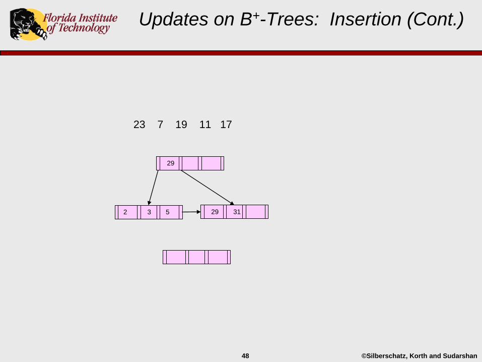
©Silberschatz, Korth and Sudarshan48
23 7 19 11 17
Updates on B+-Trees: Insertion (Cont.)
2 3 5 29 31
29
©Silberschatz, Korth and Sudarshan49
7 19 11 17
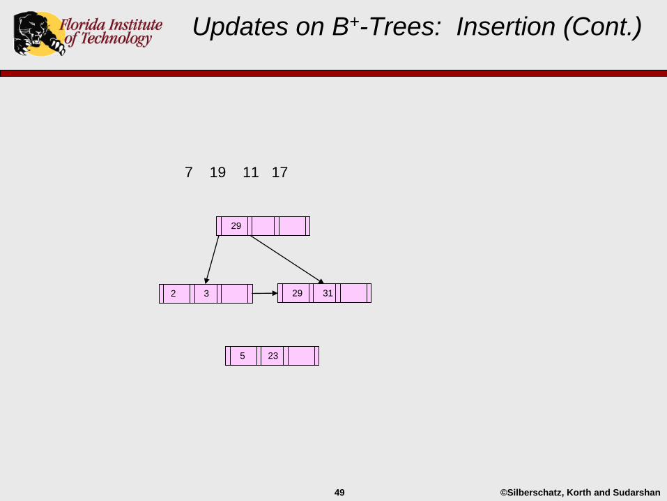
Updates on B+-Trees: Insertion (Cont.)
2 3 29 31
29
5 23

©Silberschatz, Korth and Sudarshan50
7 19 11 17
Updates on B+-Trees: Insertion (Cont.)
29 312 3 5 23
29
5
©Silberschatz, Korth and Sudarshan51
7 19 11 17
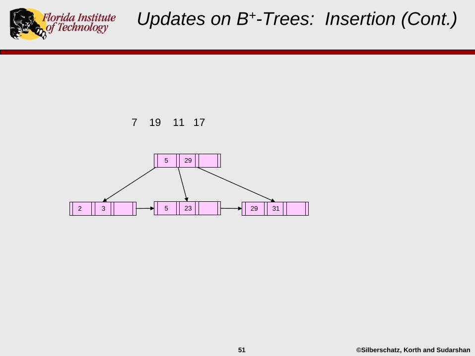
Updates on B+-Trees: Insertion (Cont.)
29 312 3 5 23
5 29
©Silberschatz, Korth and Sudarshan52
19 11 17
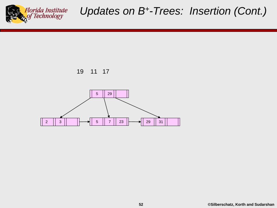
Updates on B+-Trees: Insertion (Cont.)
29 312 3 5 7 23
5 29
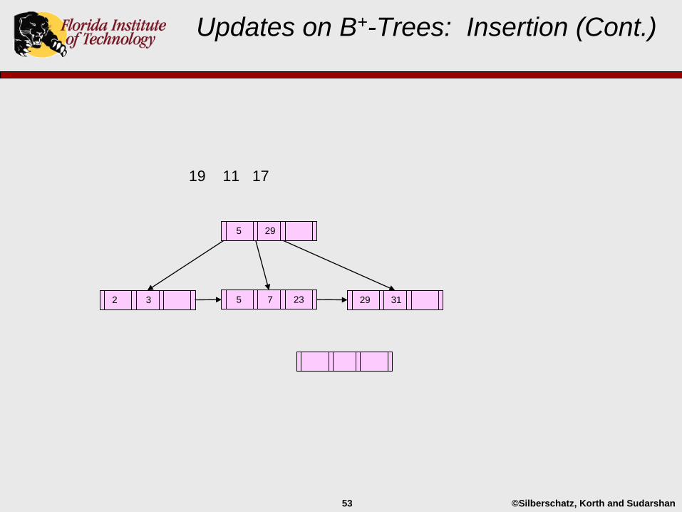
©Silberschatz, Korth and Sudarshan53
19 11 17
Updates on B+-Trees: Insertion (Cont.)
29 312 3 5 7 23
5 29
©Silberschatz, Korth and Sudarshan54
11 17
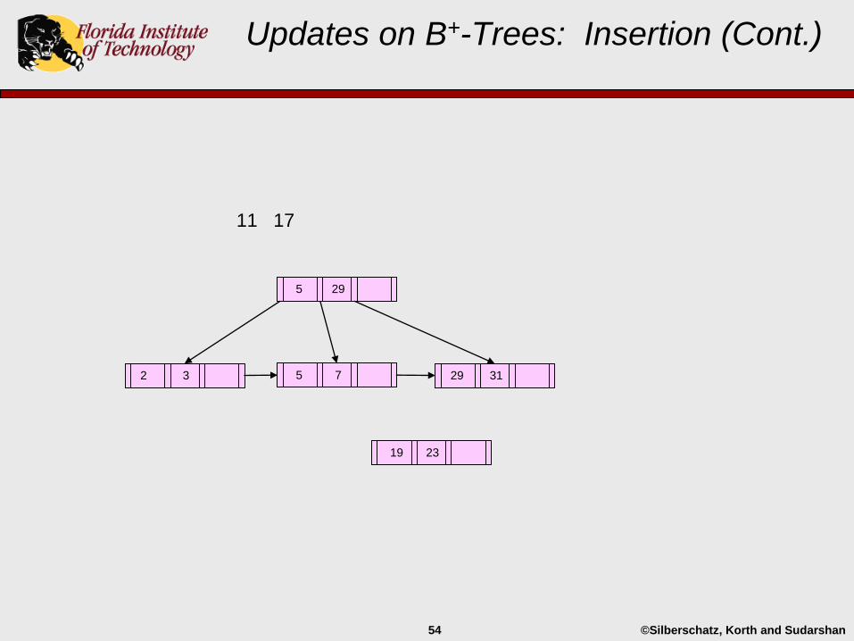
Updates on B+-Trees: Insertion (Cont.)
29 312 3 5 7
5 29
19 23
©Silberschatz, Korth and Sudarshan55
11 17
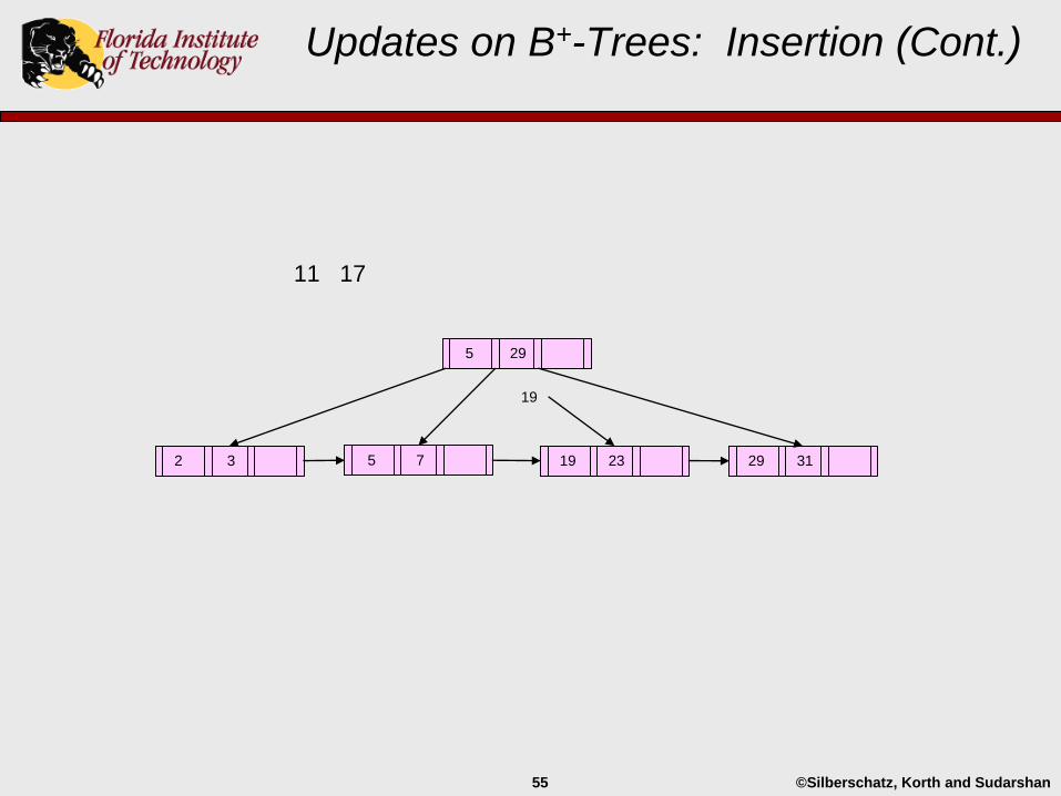
Updates on B+-Trees: Insertion (Cont.)
29 3119 232 3 5 7
5 29
19
©Silberschatz, Korth and Sudarshan56
11 17
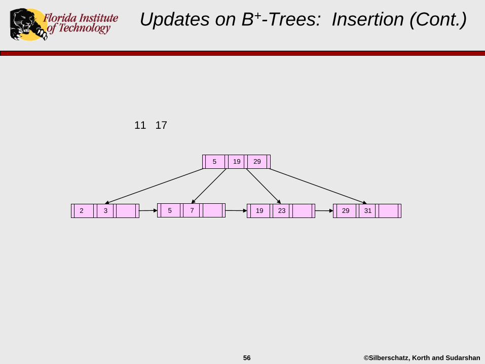
Updates on B+-Trees: Insertion (Cont.)
29 3119 232 3 5 7
5 19 29
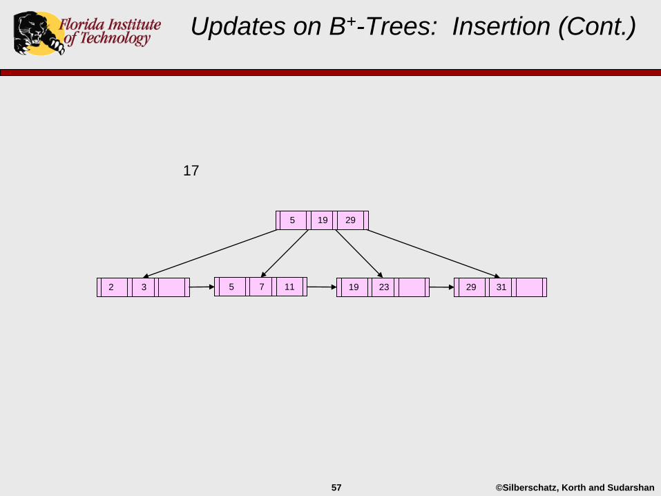
©Silberschatz, Korth and Sudarshan57
17
Updates on B+-Trees: Insertion (Cont.)
29 3119 232 3 5 7 11
5 19 29
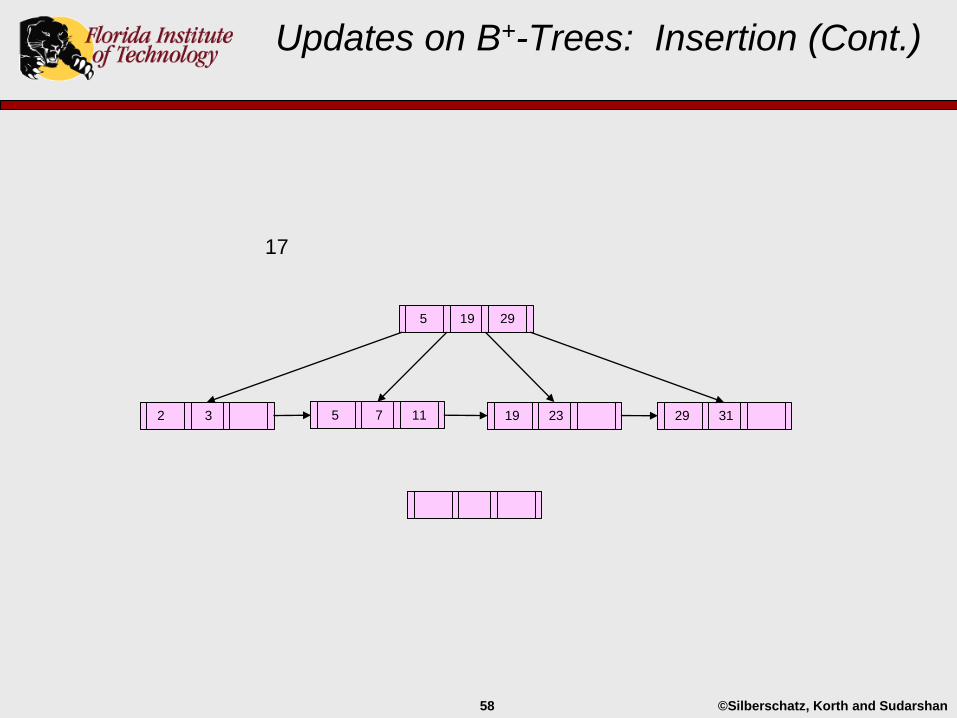
©Silberschatz, Korth and Sudarshan58
17
Updates on B+-Trees: Insertion (Cont.)
29 3119 232 3 5 7 11
5 19 29
©Silberschatz, Korth and Sudarshan59
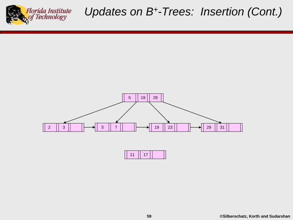
Updates on B+-Trees: Insertion (Cont.)
29 3119 232 3 5 7
5 19 29
11 17
©Silberschatz, Korth and Sudarshan60
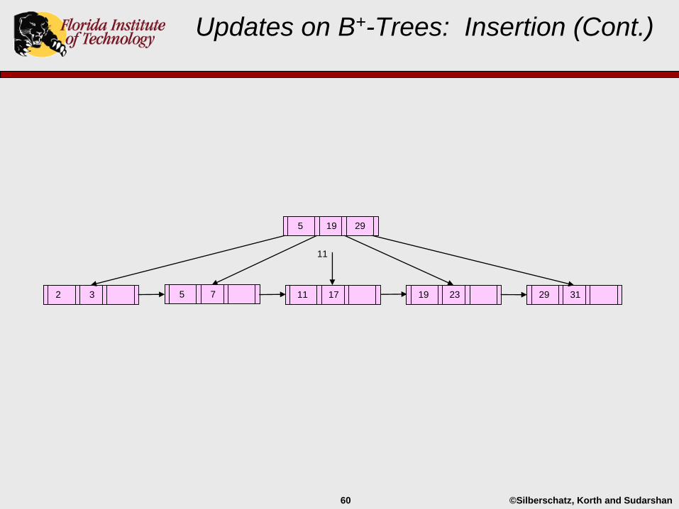
Updates on B+-Trees: Insertion (Cont.)
29 3119 232 3 5 7
5 19 29
11 17
11
©Silberschatz, Korth and Sudarshan61
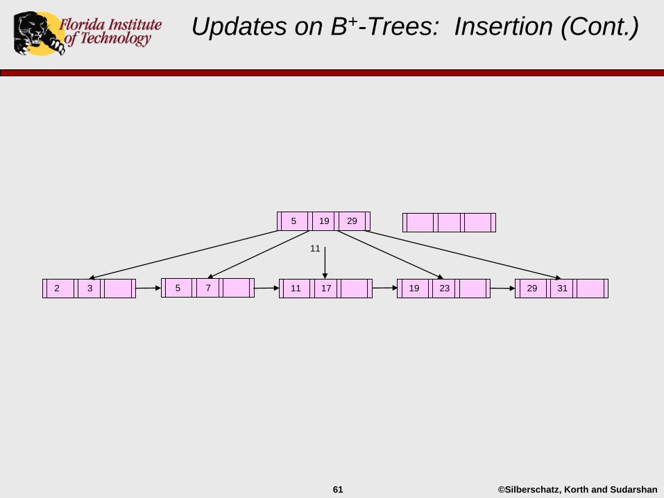
Updates on B+-Trees: Insertion (Cont.)
29 3119 232 3 5 7
5 19 29
11 17
11
©Silberschatz, Korth and Sudarshan62
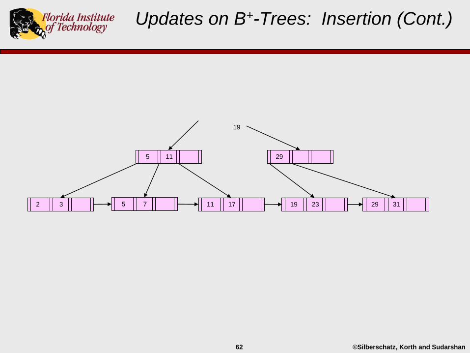
Updates on B+-Trees: Insertion (Cont.)
19 23
29
29 3111 172 3 5 7
5 11
19
©Silberschatz, Korth and Sudarshan63
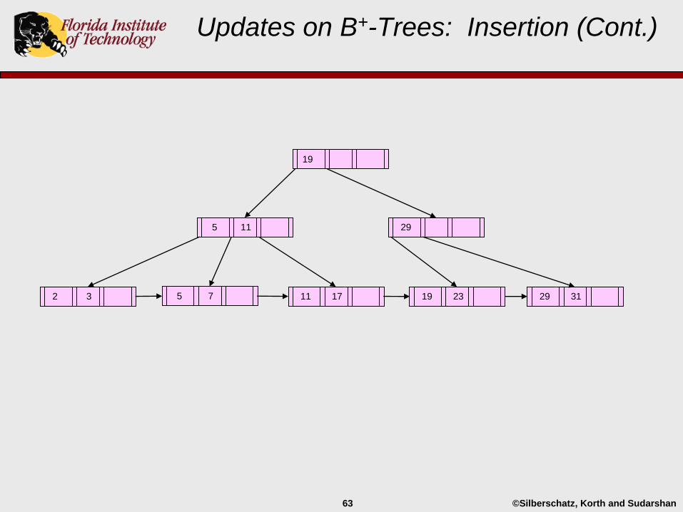
Updates on B+-Trees: Insertion (Cont.)
19
19 23
29
29 3111 172 3 5 7
5 11
©Silberschatz, Korth and Sudarshan64
Updates on B+-Trees: Deletion
Find the data record to be deleted and remove it from the data file.
If the index is a secondary index on a non-candidate key field, then delete the
corresponding pointer from the bucket.
If there are no more records with the deleted search key then remove the
search-key and pointer from the appropriate leaf node in the index.
If the node is still at least half full, then nothing more needs to be done.
If the node has too few entries, i.e., if it is less than half full, then one of two
things will happen:
merging, or
redistribution
©Silberschatz, Korth and Sudarshan65
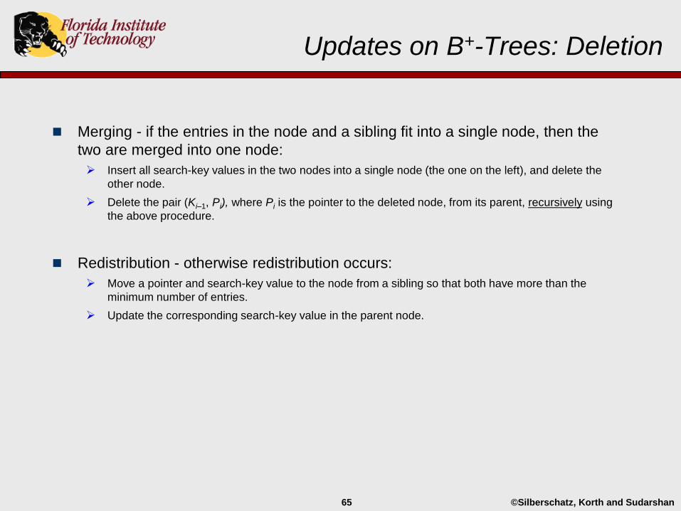
Updates on B+-Trees: Deletion
Merging - if the entries in the node and a sibling fit into a single node, then the
two are merged into one node:
Insert all search-key values in the two nodes into a single node (the one on the left), and delete the
other node.
Delete the pair (Ki–1, Pi), where Pi is the pointer to the deleted node, from its parent, recursively using
the above procedure.
Redistribution - otherwise redistribution occurs:
Move a pointer and search-key value to the node from a sibling so that both have more than the
minimum number of entries.
Update the corresponding search-key value in the parent node.
©Silberschatz, Korth and Sudarshan66
Updates on B+-Trees: Deletion
If the root node has only one pointer after deletion, it is deleted and the sole child
becomes the root.
Note that node deletions will cascade upwards until either:
a node with n/2 or more pointers is reached
redistribution with a sibling occurs, or
the root is reached.
©Silberschatz, Korth and Sudarshan67
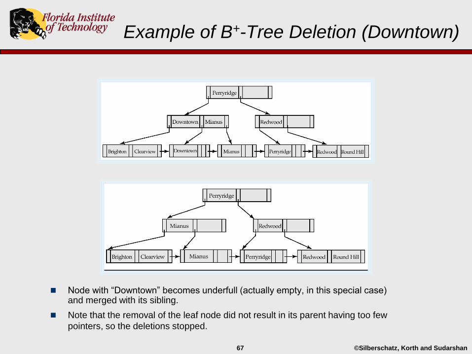
Example of B+-Tree Deletion (Downtown)
Node with “Downtown” becomes underfull (actually empty, in this special case) and merged with its sibling.
Note that the removal of the leaf node did not result in its parent having too few
pointers, so the deletions stopped.
©Silberschatz, Korth and Sudarshan68
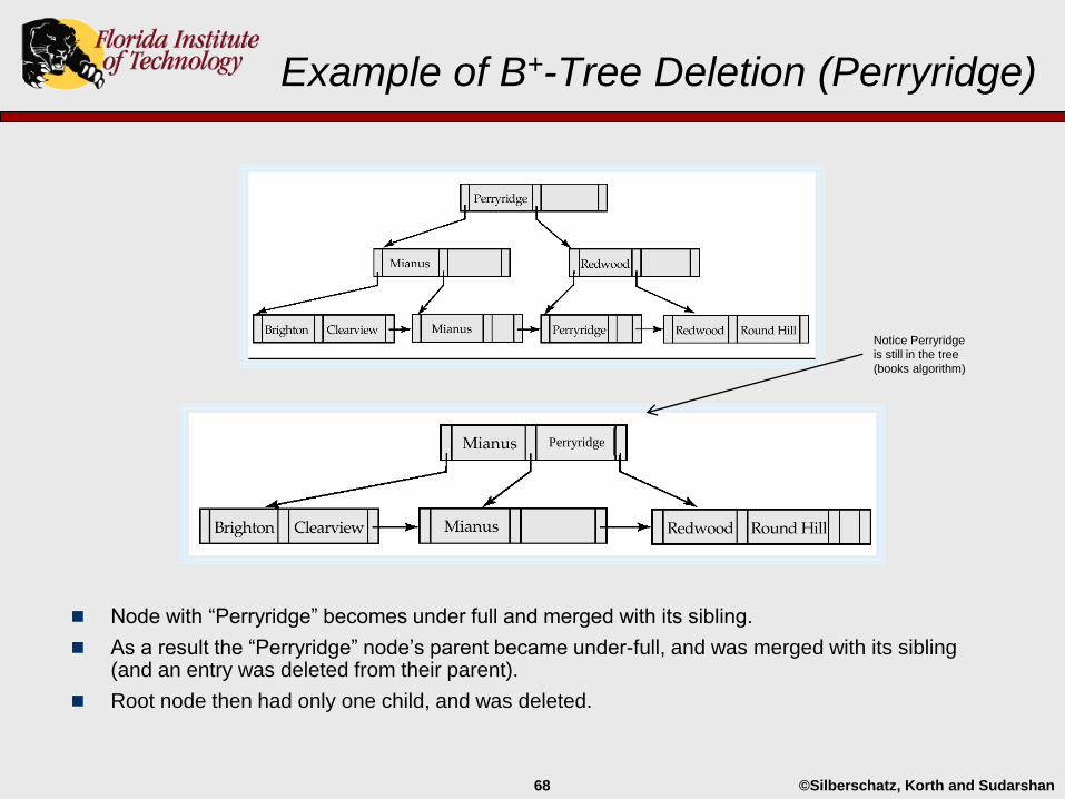
Example of B+-Tree Deletion (Perryridge)
Node with “Perryridge” becomes under full and merged with its sibling.
As a result the “Perryridge” node’s parent became under-full, and was merged with its sibling (and an entry was deleted from their parent).
Root node then had only one child, and was deleted.
Perryridge
Notice Perryridge
is still in the tree
(books algorithm)

©Silberschatz, Korth and Sudarshan69
Example of B+-tree Deletion (Perryridge)
Parent of leaf with “Perryridge” became under-full, and borrowed a pointer from its left sibling.
Search-key value in the root changes as a result.
©Silberschatz, Korth and Sudarshan70
B+-Tree File Organization
Index file degradation problem is partially solved by using B+-Tree indices (the book just says “is solved”).
Data file degradation can be similarly partially solved by using B+-Tree fileorganization (the book says “eliminated”).
Leaf nodes in a B+-tree file organization store the complete data records.
Leaf nodes are still required to be half full.
Insertion and deletion are handled in the same way as insertion and deletion of entries in a B+-tree index.
©Silberschatz, Korth and Sudarshan71
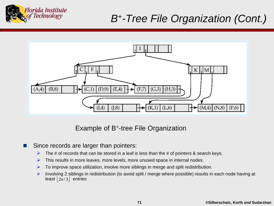
B+-Tree File Organization (Cont.)
Since records are larger than pointers:
The # of records that can be stored in a leaf is less than the # of pointers & search keys.
This results in more leaves, more levels, more unused space in internal nodes.
To improve space utilization, involve more siblings in merge and split redistribution.
Involving 2 siblings in redistribution (to avoid split / merge where possible) results in each node having at least entries
Example of B+-tree File Organization
3/2n
©Silberschatz, Korth and Sudarshan72
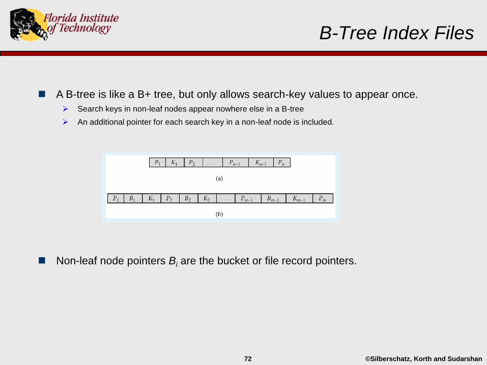
B-Tree Index Files
A B-tree is like a B+ tree, but only allows search-key values to appear once.
Search keys in non-leaf nodes appear nowhere else in a B-tree
An additional pointer for each search key in a non-leaf node is included.
Non-leaf node pointers Bi are the bucket or file record pointers.
©Silberschatz, Korth and Sudarshan73
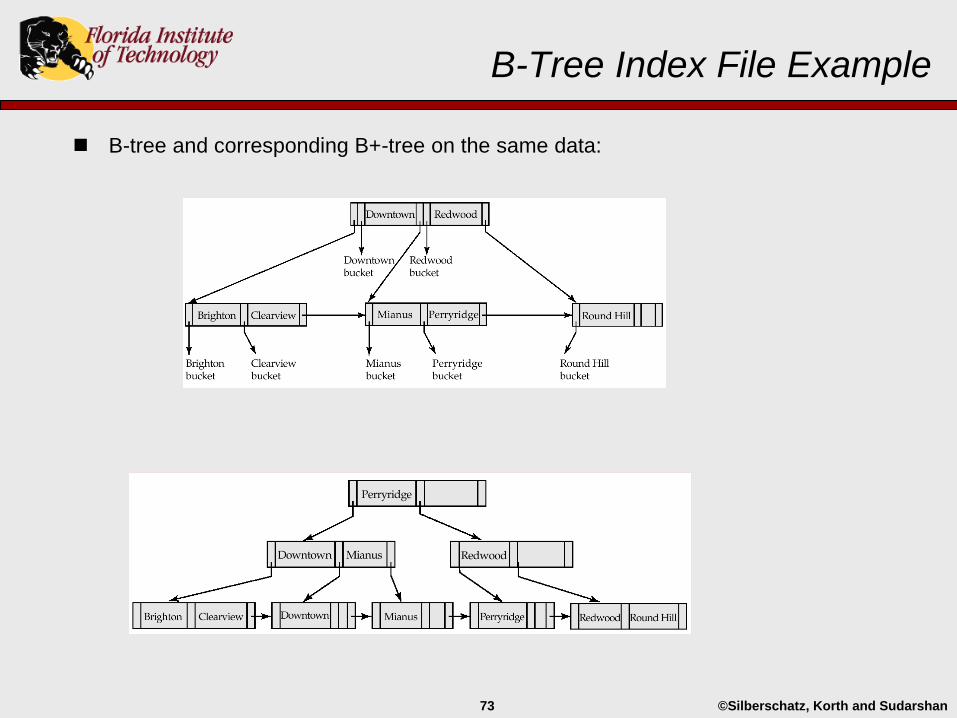
B-Tree Index File Example
B-tree and corresponding B+-tree on the same data:
©Silberschatz, Korth and Sudarshan74
B-Tree Index Files, Cont.
Advantages of B-Tree indices:
May use fewer tree nodes than a corresponding B+-Tree.
Sometimes possible to find search-key values before a reaching leaf node.
Disadvantages of B-Tree indices:
Only a “small fraction” of all search-key values are actually found early.
Non-leaf nodes contain more data, so fan-out is reduced, and thus, B-Trees typically have greater depth
than corresponding B+-Tree.
Insertion and deletion more complicated than in B+-Trees.
Every vendor has their own version.
©Silberschatz, Korth and Sudarshan75
Static Hashing
The first part of a hashing storage structure is a collection of buckets.
A bucket is a unit of storage containing one or more records.
In the simplest and ideal case a bucket is a disk block.
May contain more than one block linked together.
Every bucket has an address.
Why are they called “buckets?”
©Silberschatz, Korth and Sudarshan76
Static Hashing
The second part of a hashing storage structure is a hash function.
Just like an index, a hash function is based on a search-key:
account#
load#, payment#
A hash function h is a function from the set of all search-key values K to the set of all bucket addresses B.
Used to locate, insert and delete records.
Typically quick and easy to compute.
Typically performs a computation on the internal binary representation of the search-key.
Records with different search-keys frequently map to the same bucket.
Referred to as a “collision.”
Thus an entire bucket has to be searched sequentially to locate a record.
©Silberschatz, Korth and Sudarshan77
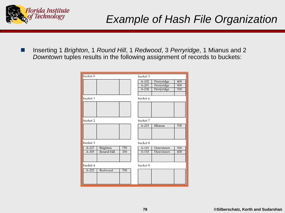
Example of Hash File Organization
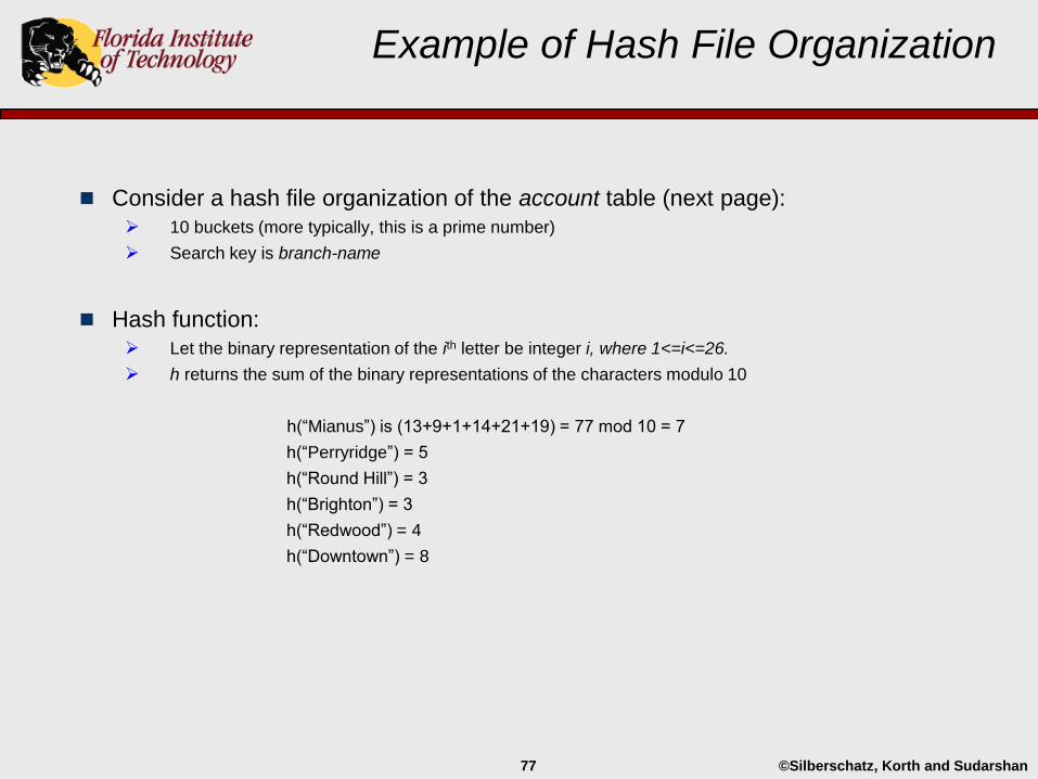
Consider a hash file organization of the account table (next page):
10 buckets (more typically, this is a prime number)
Search key is branch-name
Hash function:
Let the binary representation of the ith letter be integer i, where 1<=i<=26.
h returns the sum of the binary representations of the characters modulo 10
h(“Mianus”) is (13+9+1+14+21+19) = 77 mod 10 = 7
h(“Perryridge”) = 5
h(“Round Hill”) = 3
h(“Brighton”) = 3
h(“Redwood”) = 4
h(“Downtown”) = 8
©Silberschatz, Korth and Sudarshan78
Example of Hash File Organization
Inserting 1 Brighton, 1 Round Hill, 1 Redwood, 3 Perryridge, 1 Mianus and 2 Downtown tuples results in the following assignment of records to buckets:
©Silberschatz, Korth and Sudarshan79
Effective Hashing
In general, the goals of hashing are to:
Provide fast access to records (insertion, deletion, search)
Not waste too much space
Factors that contribute to achieving these goals:
Having a “good” hash function
Have the right number of buckets; not too many, not too few
Lots of in-depth mathematical research has gone into the analysis of hashing and hash function…most of which will not be covered here.
Other (algorithms) textbooks cover hashing and hash functions to a much greater degree.
©Silberschatz, Korth and Sudarshan80
Hash Functions
Ideal hash function is uniform - each bucket is assigned the same number of search-key values from the set of all possible search keys.
Ideal hash function is random - on average each bucket will have the same number of records assigned to it irrespective of the actual distribution of search-key values in the file.
A uniform hash function is not necessarily random, and visa-versa.
©Silberschatz, Korth and Sudarshan81
Hash Functions
Example – storing employees in buckets based on salary (uniform but not random):
bucket 0: 0-19k
bucket 1: 20k-39k
bucket 2: 40k-59k
bucket 3: 60k-79k
bucket 4: 80k-99k
Ranges can be adjusted to be more random, but then the hash function is not uniform.
In general, designing a (truly) random hash function is difficult:
Only possible if each search key value is in a small fraction of records.
Worst case – hash function maps all search-key values to the same bucket; this makes access time proportional to the number of search-key values in the file.
©Silberschatz, Korth and Sudarshan82
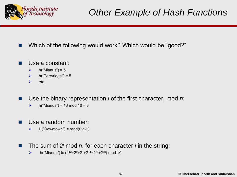
Other Example of Hash Functions
Which of the following would work? Which would be “good?”
Use a constant: h(“Mianus”) = 5
h(“Perryridge”) = 5
etc.
Use the binary representation i of the first character, mod n: h(“Mianus”) = 13 mod 10 = 3
Use a random number: H(“Downtown”) = rand(0:n-1)
The sum of 2i mod n, for each character i in the string: h(“Mianus”) is (213+29+21+214+221+219) mod 10

©Silberschatz, Korth and Sudarshan83
Bucket Overflows
Goal – one block per bucket.
Bucket overflow occurs when a bucket has been assigned more records than it has space for.
Bucket overflow can occur because of:
Insufficient buckets - lots of records
Skew in record distribution across buckets
• multiple records have same search-key value
• bad hash function (non-random distribution)
• non-prime number of buckets*
The probability of bucket overflow can be reduced, but not eliminated.
Overflow is handled by chaining overflow blocks.
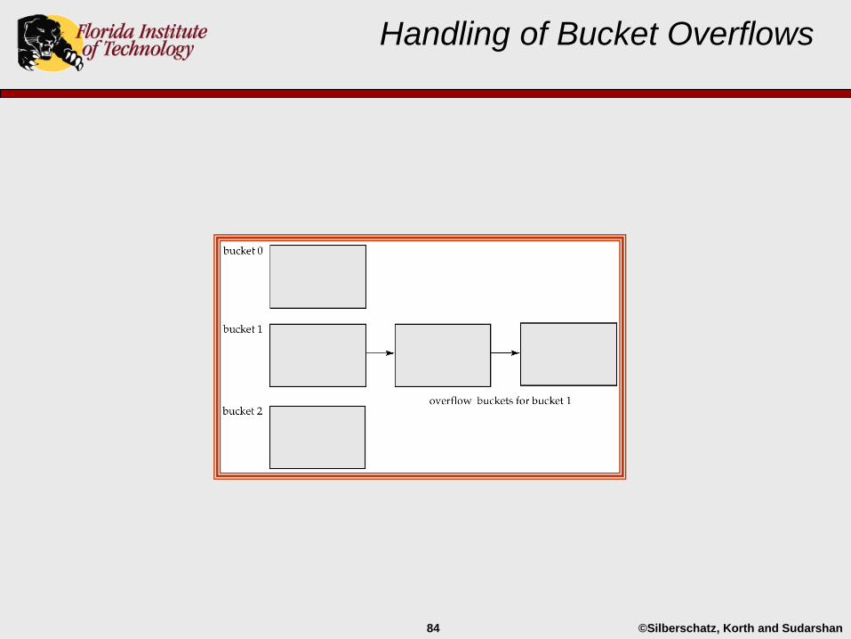
©Silberschatz, Korth and Sudarshan84
Handling of Bucket Overflows

©Silberschatz, Korth and Sudarshan85
The Number of Buckets
So what should the number of buckets be?
More buckets:
fewer collisions
less chaining
better performance
more wasted/unused space.
Fewer buckets:
more collisions
more chaining
worse performance
less wasted/unused space.
©Silberschatz, Korth and Sudarshan86
The Number of Buckets
Let n be the number of records to be stored, and let k be the maximum number of records that can be stored in a block.
At least n/k buckets are necessary to avoid chaining.
A common recommendation is for the number of buckets to be the smallest prime number bwhere:
b > n/k*1.2
This ensues that the number of buckets is slightly bigger (20%) than the minimum # required.
©Silberschatz, Korth and Sudarshan87
Hash Indices
As described, hashing is used to organize a data file, and does not provide an
index structure, per se.
It does however, provide the benefits of an index, i.e., fast access.
Hashing can, however, be used for an index file as well.
Strictly speaking, a hash index organizes the search keys, with their associated
record pointers, into a hash file structure.
That having been said, the phrase hash index is used to denote both uses.
©Silberschatz, Korth and Sudarshan88
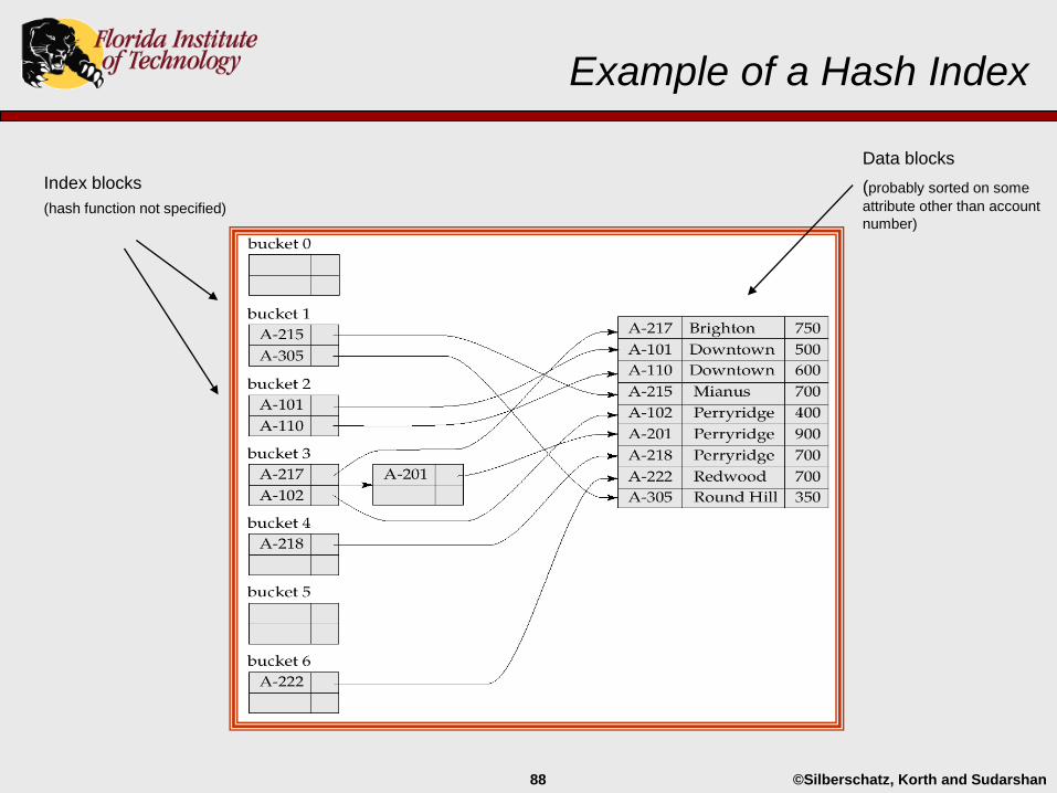
Example of a Hash Index
Index blocks
(hash function not specified)
Data blocks
(probably sorted on some
attribute other than account
number)
©Silberschatz, Korth and Sudarshan89
Hash Indices, Cont.
The book says that “strictly speaking, hash indices are always secondary indices.”
This raises the following question:
Would a hash index make sense on an attribute on which the table is sorted?
If so, then, by definition that index would be a primary index, thereby contradicting the above.
Why the heck not?
Perhaps the point the authors were trying to make is:
If data records are assigned to blocks using hashing, then the table is not sorted by the search key, so it can’t be referred to as a primary index.
©Silberschatz, Korth and Sudarshan90
Performance of Hashing
Point querys:
O(1) best case
O(n) worst case
O(1) average case
Range queries:
Not possible with a hash organization or index
How does this compare with B+-trees?
Hashing optimizes average-case performance at the expense of worst-case performance.
B+-trees optimize worst-case performance at the expense of best-case and average case performance.
©Silberschatz, Korth and Sudarshan91
Deficiencies of Static Hashing
In static hashing h maps search-key values to a fixed set of buckets.
If initial # of buckets is too small, performance degrades due to overflows as the database grows.
If file size in the future is anticipated and the number of buckets allocated accordingly, significant amount of space will be wasted initially.
If the database shrinks, again space will be wasted.
One option is periodic re-organization of the file with a new hash function, but this can be expensive.
These problems can be avoided by using techniques that allow the number of buckets to be modified dynamically.

©Silberschatz, Korth and Sudarshan92
Extendable Hashing
Good for databases that grow and shrink in size (dramatically).
The hash function and number of buckets change dynamically.
An extendable hash table has three parts: Hash function
Buckets
Bucket address table

©Silberschatz, Korth and Sudarshan93
Dynamic Hashing – Hash Function
Hash function:
Generates values over a large range.
Typically b-bit integers, with b = 32.
Wow! That’s a lot of buckets!
At any time, only a prefix of the hash function is used.
The length of the prefix used is i bits, 0 i b.
i is referred to as the global depth
The value of i, will grow and shrink along with the hash table.
i is used to index into the bucket address table
©Silberschatz, Korth and Sudarshan94
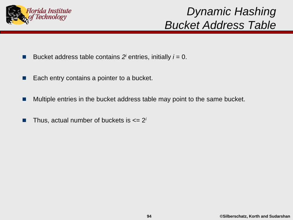
Dynamic Hashing
Bucket Address Table
Bucket address table contains 2i entries, initially i = 0.
Each entry contains a pointer to a bucket.
Multiple entries in the bucket address table may point to the same bucket.
Thus, actual number of buckets is <= 2i
©Silberschatz, Korth and Sudarshan95
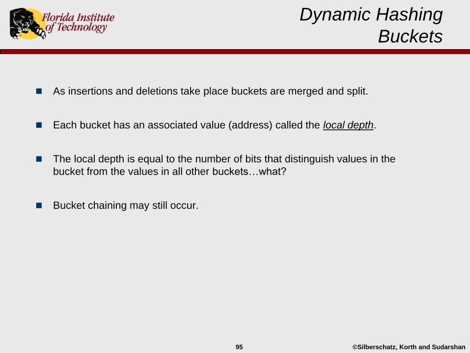
Dynamic Hashing
Buckets
As insertions and deletions take place buckets are merged and split.
Each bucket has an associated value (address) called the local depth.
The local depth is equal to the number of bits that distinguish values in the
bucket from the values in all other buckets…what?
Bucket chaining may still occur.
©Silberschatz, Korth and Sudarshan96
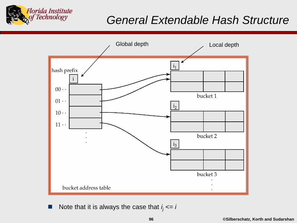
General Extendable Hash Structure
Note that it is always the case that ij <= i
Global depth Local depth
©Silberschatz, Korth and Sudarshan97
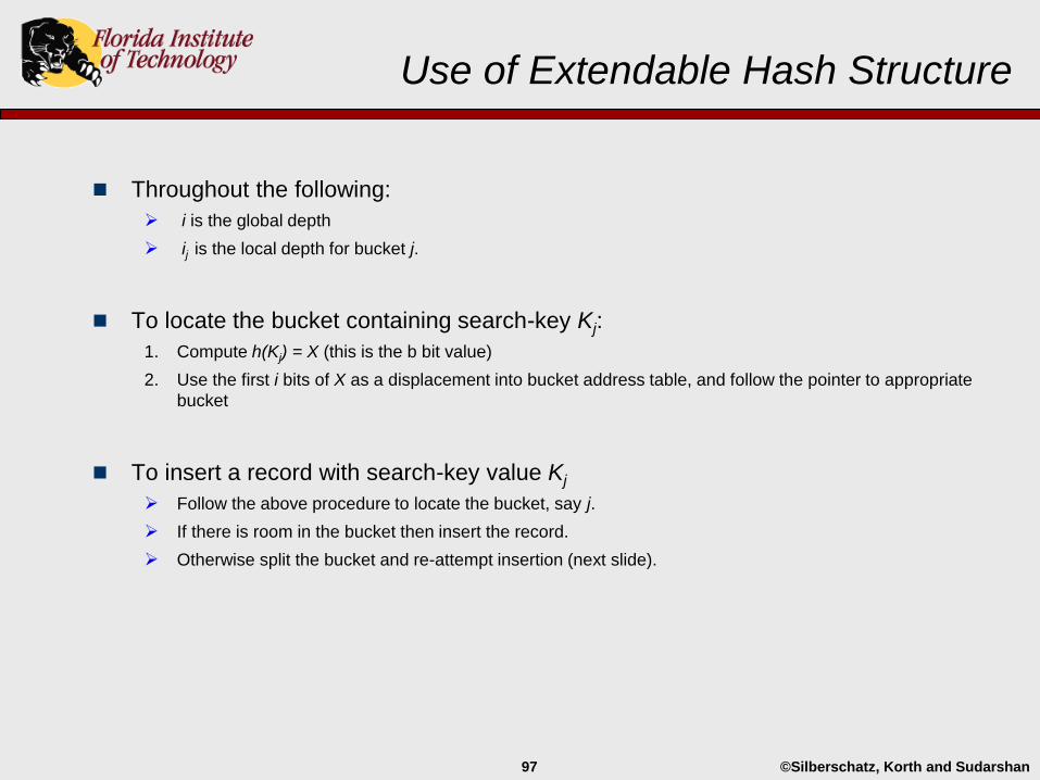
Use of Extendable Hash Structure
Throughout the following:
i is the global depth
ij is the local depth for bucket j.
To locate the bucket containing search-key Kj:
1. Compute h(Kj) = X (this is the b bit value)
2. Use the first i bits of X as a displacement into bucket address table, and follow the pointer to appropriate
bucket
To insert a record with search-key value Kj
Follow the above procedure to locate the bucket, say j.
If there is room in the bucket then insert the record.
Otherwise split the bucket and re-attempt insertion (next slide).
©Silberschatz, Korth and Sudarshan98
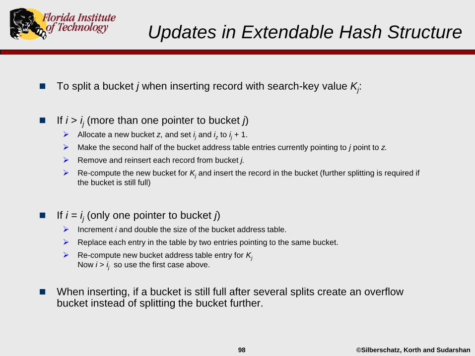
Updates in Extendable Hash Structure
To split a bucket j when inserting record with search-key value Kj:
If i > ij (more than one pointer to bucket j)
Allocate a new bucket z, and set ij and iz to ij + 1.
Make the second half of the bucket address table entries currently pointing to j point to z.
Remove and reinsert each record from bucket j.
Re-compute the new bucket for Kj and insert the record in the bucket (further splitting is required if
the bucket is still full)
If i = ij (only one pointer to bucket j)
Increment i and double the size of the bucket address table.
Replace each entry in the table by two entries pointing to the same bucket.
Re-compute new bucket address table entry for Kj
Now i > ij so use the first case above.
When inserting, if a bucket is still full after several splits create an overflow bucket instead of splitting the bucket further.
©Silberschatz, Korth and Sudarshan99
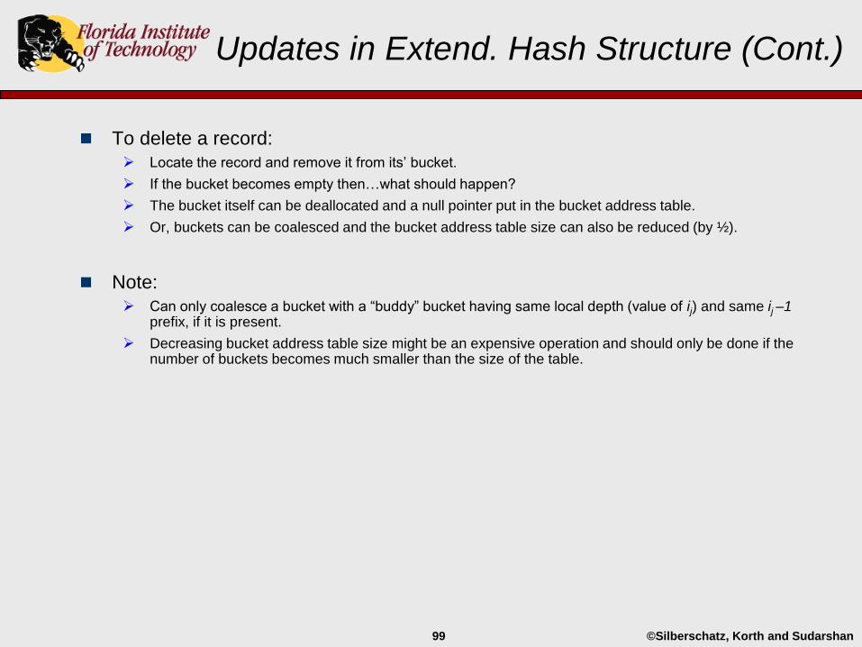
Updates in Extend. Hash Structure (Cont.)
To delete a record:
Locate the record and remove it from its’ bucket.
If the bucket becomes empty then…what should happen?
The bucket itself can be deallocated and a null pointer put in the bucket address table.
Or, buckets can be coalesced and the bucket address table size can also be reduced (by ½).
Note:
Can only coalesce a bucket with a “buddy” bucket having same local depth (value of ij) and same ij –1prefix, if it is present.
Decreasing bucket address table size might be an expensive operation and should only be done if the number of buckets becomes much smaller than the size of the table.
©Silberschatz, Korth and Sudarshan100
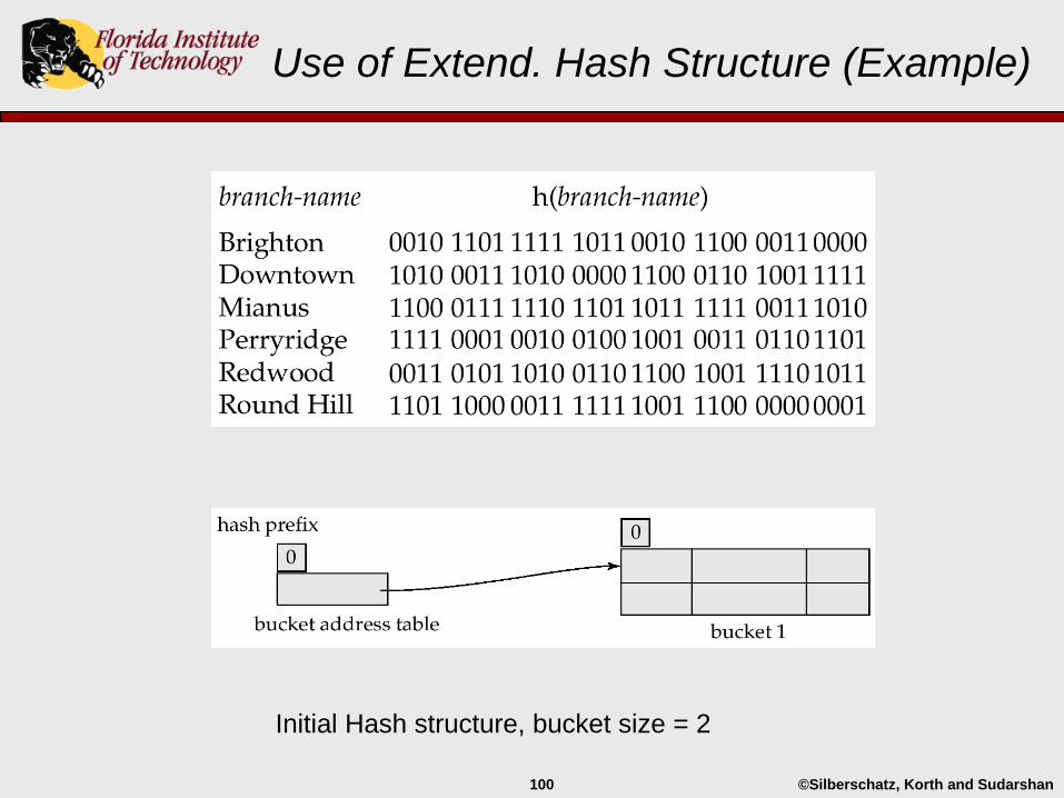
Use of Extend. Hash Structure (Example)
Initial Hash structure, bucket size = 2
©Silberschatz, Korth and Sudarshan101
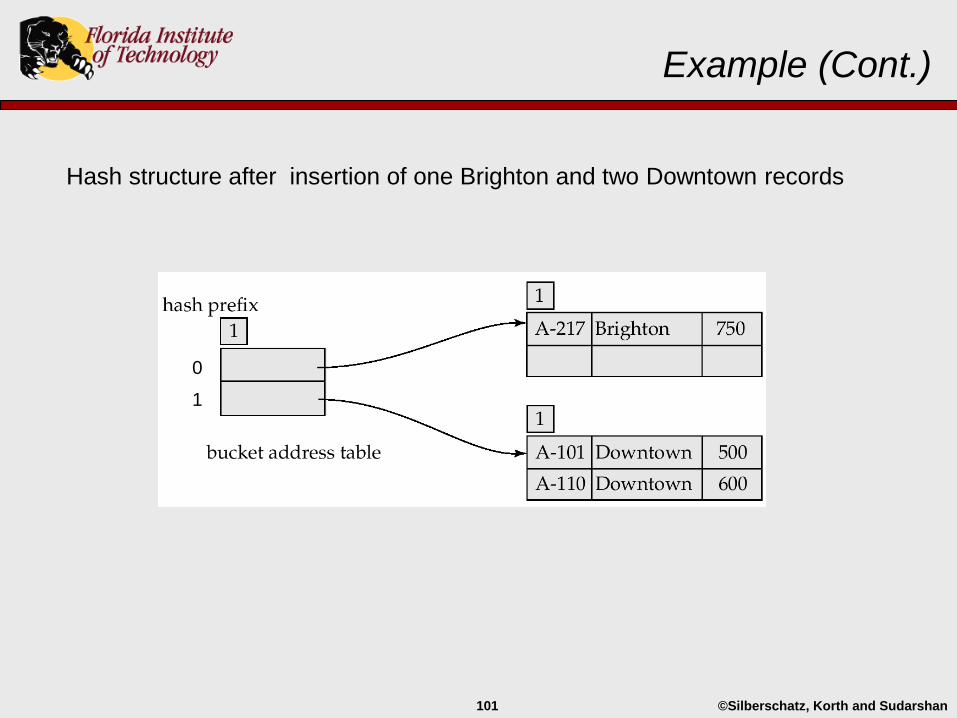
Example (Cont.)
Hash structure after insertion of one Brighton and two Downtown records
0
1
©Silberschatz, Korth and Sudarshan102
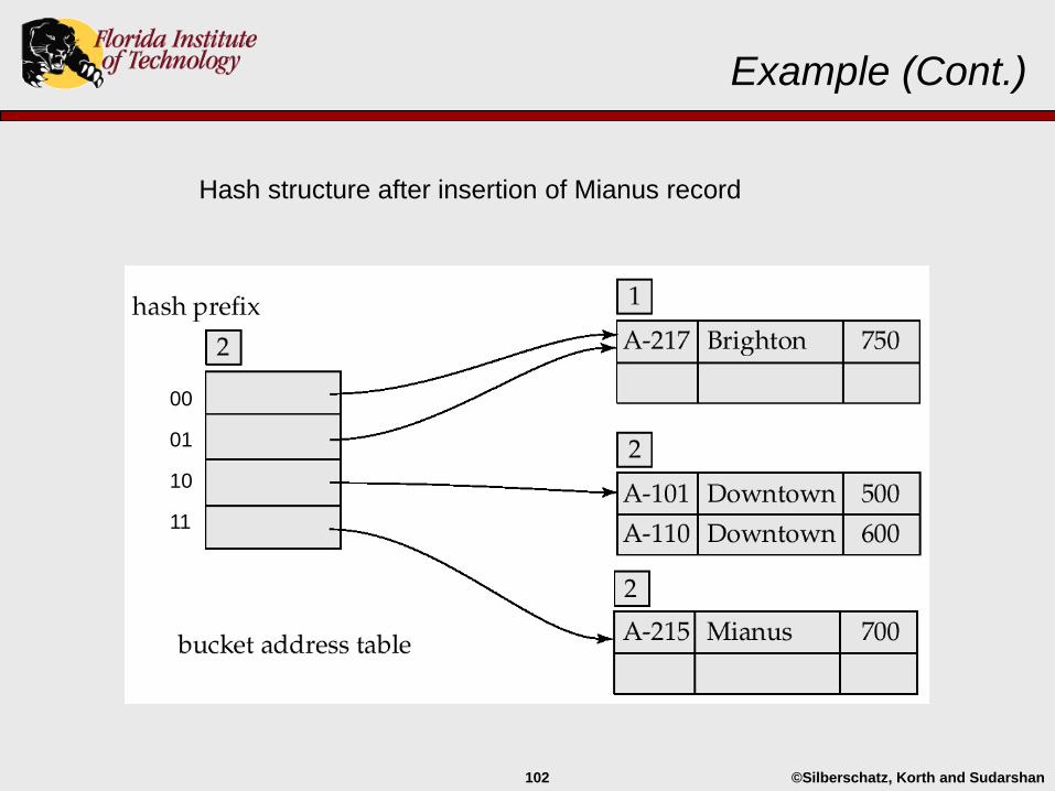
Example (Cont.)
Hash structure after insertion of Mianus record
00
01
10
11
©Silberschatz, Korth and Sudarshan103
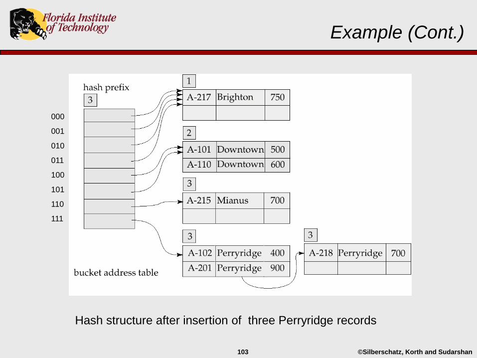
Example (Cont.)
Hash structure after insertion of three Perryridge records
000
001
010
011
100
101
110
111
©Silberschatz, Korth and Sudarshan104
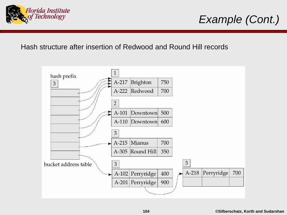
Example (Cont.)
Hash structure after insertion of Redwood and Round Hill records
©Silberschatz, Korth and Sudarshan105
Extendable Hashing vs. Other Schemes
Benefits of extendable hashing:
Chaining is reduced, so performance does not degrade with file growth.
Minimal space overhead (?).
Disadvantages of extendable hashing:
Extra level of indirection to find desired record.
Bucket address table may itself become larger than memory.
• Could impose a tree (or other) structure to locate an index entry.
Changing the size of bucket address table can be an expensive operation.
©Silberschatz, Korth and Sudarshan106
Bitmap Indices
Bitmap indices are a special type of index designed for efficient querying on multiple search keys:
Not particularly useful for single attribute queries
Typically used in data warehouses
Applicable on attributes having a small number of distinct values:
State, country, gender…
Income-level (0-9999, 10000-19999, 20000-50000, 50000-infinity)
Bitmap assumptions:
Records in a relation are numbered sequentially from, say, 0
Given a number n it must be easy (i.e., formulaic) to retrieve record n; particularly easy if records are of fixed size
Records do not move
©Silberschatz, Korth and Sudarshan107
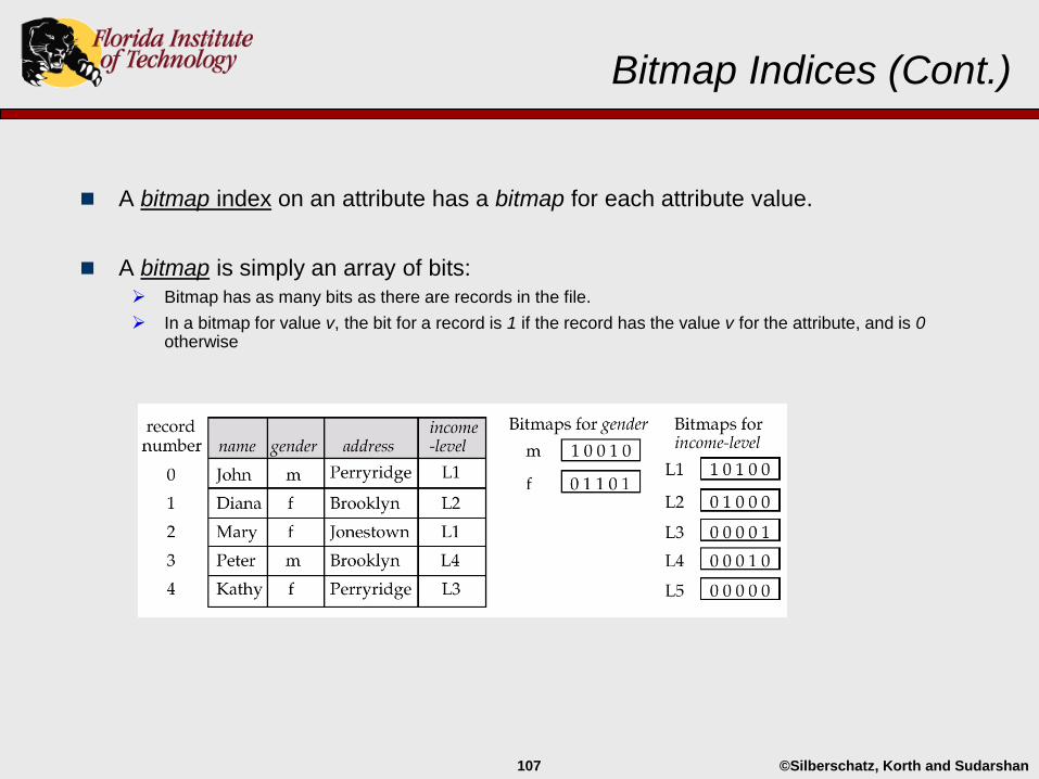
Bitmap Indices (Cont.)
A bitmap index on an attribute has a bitmap for each attribute value.
A bitmap is simply an array of bits:
Bitmap has as many bits as there are records in the file.
In a bitmap for value v, the bit for a record is 1 if the record has the value v for the attribute, and is 0otherwise
©Silberschatz, Korth and Sudarshan108
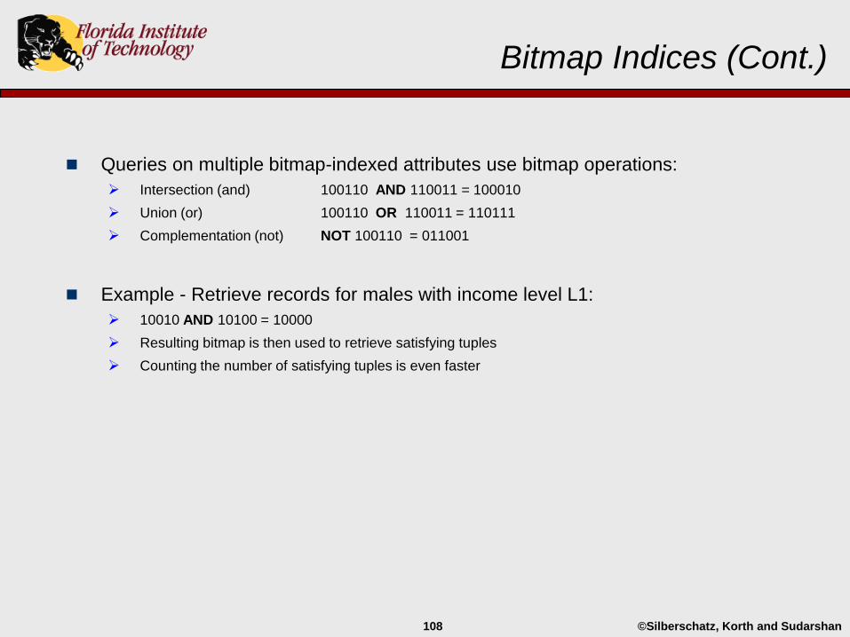
Bitmap Indices (Cont.)
Queries on multiple bitmap-indexed attributes use bitmap operations:
Intersection (and) 100110 AND 110011 = 100010
Union (or) 100110 OR 110011 = 110111
Complementation (not) NOT 100110 = 011001
Example - Retrieve records for males with income level L1:
10010 AND 10100 = 10000
Resulting bitmap is then used to retrieve satisfying tuples
Counting the number of satisfying tuples is even faster
©Silberschatz, Korth and Sudarshan109
Bitmap Indices (Cont.)
Bitmap indices are generally very small compared with relation size.
Example:
number of records is n
record size 100 bytes, i.e., 800 bits (somewhat conservative)
total table size is n * 800 bits
bitmap size is n bits
space for a single bitmap is 1/800 of space used by the relation.
If the number of distinct attribute values is 8, then the bitmap index is only 1% of
relation size (e.g., 1TB table, 10GB bitmap index).
Exercise (do the math) - What happens if each record is 32 bits and there are 64
distinct attribute values? Where is the cut-off point?
©Silberschatz, Korth and Sudarshan110
Bitmap Indices (Cont.)
How does a bitmap change if a record is deleted? Could we simply put a 0 in all bitmaps for the record?
Consider the predicate term:
NOT (branch-name = “perryridge”)
An existence bitmap could be used to indicate if there is a valid record at a specific location for negation to
work properly.
(NOT (branch-name = “perryridge”)) AND Existence-Bitmap
©Silberschatz, Korth and Sudarshan111
Bitmap Indices (Cont.)
Bitmaps need to be maintained for all values, including null:
To correctly handle SQL null semantics for NOT(Attribute = value): Intersect the above result with (NOT A-null-bitmap)
(NOT (branch-name = “perryridge”))
AND Existence-Bitmap AND (NOT branch-name-null-bitmap)
©Silberschatz, Korth and Sudarshan112
Efficient Implementation of Bitmap Operations
The bits in a bitmap are packed tightly together, i.e., into words.
A single word and operation (alternatively an or; both CPU operations) computes the and of 32 or 64 bits at once.
The conjunction of two bitmaps containing 1-million-bits can thus be done with just 31,250 instructions.
©Silberschatz, Korth and Sudarshan113
Efficient Implementation of Bitmap Operations
Similarly, counting the number of 1s can be done fast by a trick:
Use each byte to index into a pre-computed array of 256 elements each storing the count of 1s in the binary representation.
Add up retrieved counts
Bitmaps can be used instead of Tuple-ID lists at the leaf level of a B+-tree, for values that have a large number of matching records.
If a tuple-id (pointer) is 64-bits, then this saves space if > 1/64 of the records have a specific value (exercise - do the math).
©Silberschatz, Korth and Sudarshan114
Index Definition in SQL
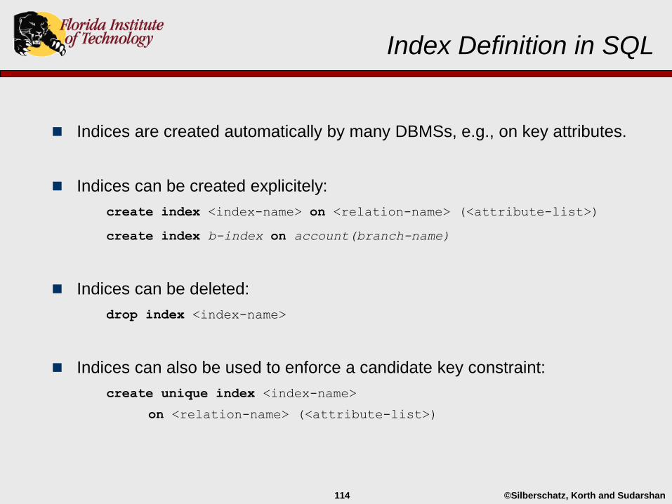
Indices are created automatically by many DBMSs, e.g., on key attributes.
Indices can be created explicitely:
create index <index-name> on <relation-name> (<attribute-list>)
create index b-index on account(branch-name)
Indices can be deleted:
drop index <index-name>
Indices can also be used to enforce a candidate key constraint:
create unique index <index-name>
on <relation-name> (<attribute-list>)
©Silberschatz, Korth and Sudarshan115
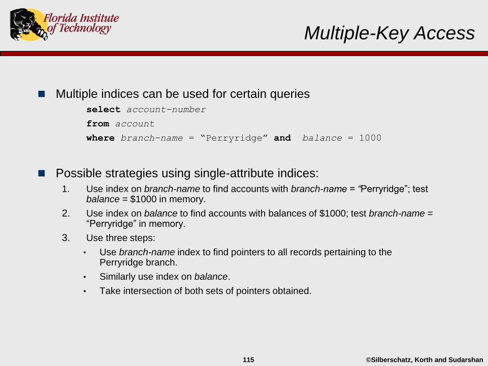
Multiple-Key Access
Multiple indices can be used for certain queriesselect account-number
from account
where branch-name = “Perryridge” and balance = 1000
Possible strategies using single-attribute indices:
1. Use index on branch-name to find accounts with branch-name = “Perryridge”; test balance = $1000 in memory.
2. Use index on balance to find accounts with balances of $1000; test branch-name = “Perryridge” in memory.
3. Use three steps:
• Use branch-name index to find pointers to all records pertaining to the Perryridge branch.
• Similarly use index on balance.
• Take intersection of both sets of pointers obtained.

©Silberschatz, Korth and Sudarshan116
Indices on Multiple Attributes
A single index can be created on more than one attribute.
Ordered or hash-based
A key requirement for ordered indices is the ability to compare
search keys for =, < and >.
Suppose a multi-attribute ordered index is created on the attributes
(branch-name, balance) in the branch relation.
How do comparisons work?
=, <, >, etc.
©Silberschatz, Korth and Sudarshan117
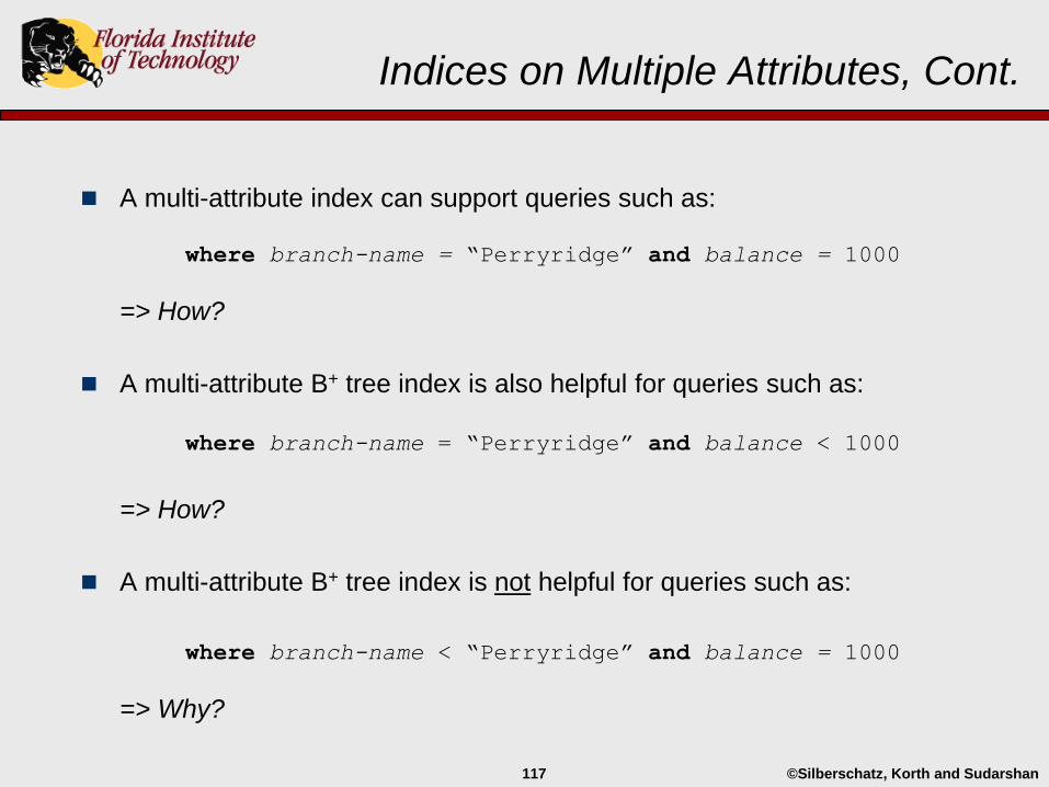
Indices on Multiple Attributes, Cont.
A multi-attribute index can support queries such as:
where branch-name = “Perryridge” and balance = 1000
=> How?
A multi-attribute B+ tree index is also helpful for queries such as:
where branch-name = “Perryridge” and balance < 1000
=> How?
A multi-attribute B+ tree index is not helpful for queries such as:
where branch-name < “Perryridge” and balance = 1000
=> Why?

©Silberschatz, Korth and Sudarshan118
End of Chapter
©Silberschatz, Korth and Sudarshan119
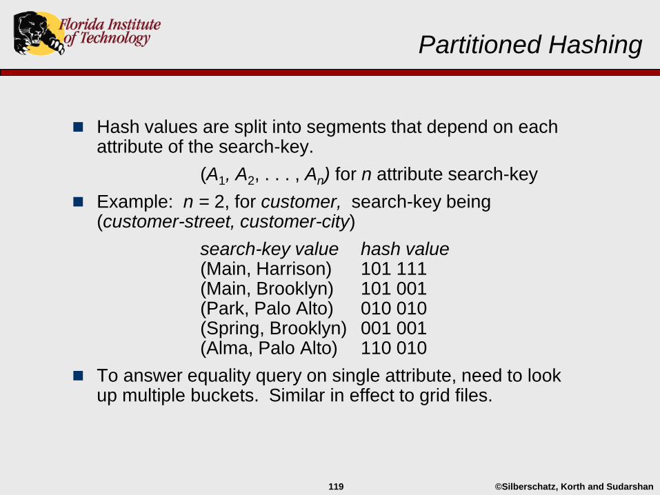
Partitioned Hashing
Hash values are split into segments that depend on each attribute of the search-key.
(A1, A2, . . . , An) for n attribute search-key
Example: n = 2, for customer, search-key being (customer-street, customer-city)
search-key value hash value(Main, Harrison) 101 111(Main, Brooklyn) 101 001(Park, Palo Alto) 010 010(Spring, Brooklyn) 001 001(Alma, Palo Alto) 110 010
To answer equality query on single attribute, need to look up multiple buckets. Similar in effect to grid files.
©Silberschatz, Korth and Sudarshan120
Grid Files
A grid file is an index that supports multiple search-key
queries involving one or more comparison operators.
The grid file consists of:
a single n-dimensional grid array, where n is the number of
search key attributes.
n linear scales, one for each search-key attribute.
Multiple cells of grid array can point to same bucket.
©Silberschatz, Korth and Sudarshan121
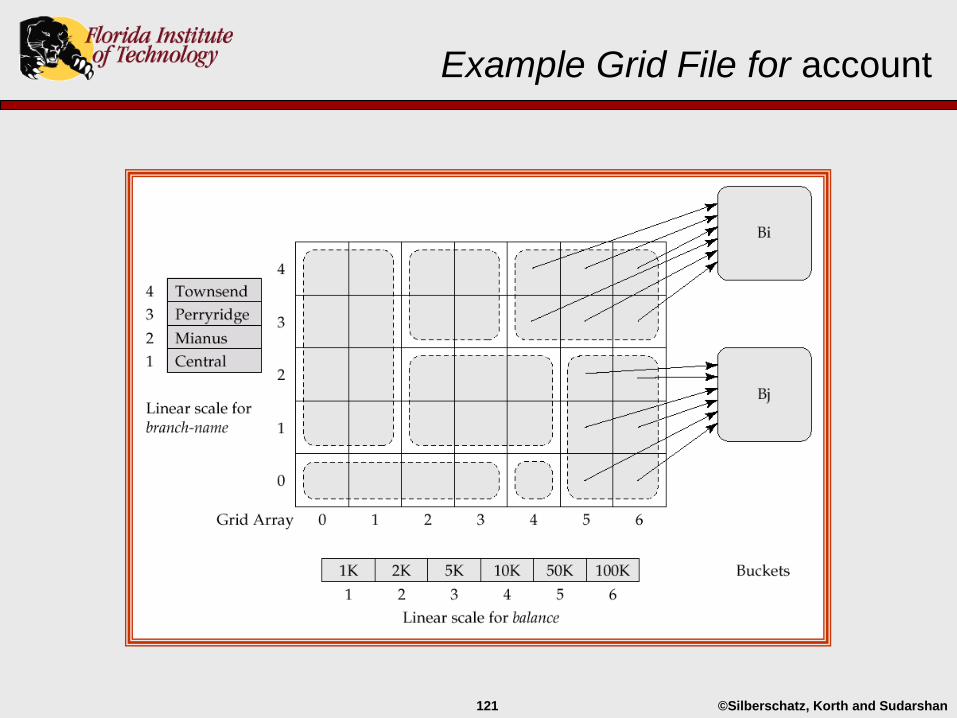
Example Grid File for account
©Silberschatz, Korth and Sudarshan122
Queries on a Grid File
A grid file on two attributes A and B can handle queries of all following
forms with reasonable efficiency
(a1 A a2)
(b1 B b2)
(a1 A a2 b1 B b2)
During insertion: (Similar to extendable hashing, but on n dimensions)
If a bucket becomes full then it can be split if more than one cell points to it.
If only one cell points to the bucket, either an overflow bucket can be created
or the grid size can be increased
During deletion: (Also similar to extendable hashing)
If a bucket becomes empty, the bucket can be merged with other buckets
Or the grid pointer can be set to null, etc.
©Silberschatz, Korth and Sudarshan123
Grid Files (Cont.)
Linear scales must be chosen to uniformly distribute records
across cells.
Otherwise there will be too many overflow buckets.
Periodic re-organization to increase grid size will help.
But reorganization can be very expensive.
Space overhead of grid array can be high.
R-trees (Chapter 23) are an alternative