Increasing Supply Chain Robustness through Process ...

Increasing Supply Chain Robustness through

Process Flexibility and Strategic Inventory

by

He Wang

B.Eng. Industrial Engineering, B.S. MathematicsTsinghua University, 2011

ARCHfVLMASSACHUSETTS INS UYE

OF TECHNOLOGY

JUL 0 8 2013

LIBRARIES

Submitted to the Department of Civil and Environmental Engineeringin partial fulfillment of the requirements for the degree of

Master of Science in Transportation

at the

MASSACHUSETTS INSTITUTE OF TECHNOLOGY

June 2013

© 2013 Massachusetts Institute of Technology. All rights reserved.

Author ........................ ..... ....................Department of Civil and Environmental Engineering

May 9, 2013

Certified by............................................David Simchi-Levi

Professor of Civil and Environmental Engineering and EngineeringSystems

ThesA Supervistr

A ccepted by ...........................

Chair, Departmental Committee for Graduate Students

I IHeidi M. Nepf

Increasing Supply Chain Robustness through Process

Flexibility and Strategic Inventory

by

He Wang

Submitted to the Department of Civil and Environmental Engineeringon May 9, 2013, in partial fulfillment of the

requirements for the degree ofMaster of Science in Transportation

Abstract

When a disruption brings down one of company's manufacturing facilities, it canhave a ripple effect on the entire supply chain and threaten the company's abilityto compete. In this thesis, we develop an effective disruption mitigation strategyby using both process flexibility and strategic inventory. The model is focused ona manufacturer with multiple plants producing multiple products, where strategicinventory can be held for any product. We propose a new metric of supply chainrobustness, defined as the maximum time that no customer demand is lost regardlessof which plant is disrupted.

Using this metric, we analyze K-chain flexibility designs in which each plant iscapable of producing exactly K products. It is demonstrated that a 2-chain design,which is known to be effective for matching supply with demand when there is nodisruption, is not robust when there is both disruption and demand uncertainty.However, it is shown that a 3-chain design is significantly more robust and achievesthe same robustness as full flexibility under high uncertainty level.

We then extend the model to an assembly system and find that investment in pro-cess flexibility designs changes the optimal inventory placements. In particular, whenthe degree of flexibility is high, more inventory is allocated to standard components,i.e. components used by multiple products, but when the degree of flexibility is low,more inventory is allocated to non-standard components.

Thesis Supervisor: David Simchi-LeviTitle: Professor of Civil and Environmental Engineering and Engineering Systems

Acknowledgments

I would like to acknowledge the Department of Civil and Environmental Engineering

for taking me to MIT, and for allowing me to pursue this adventure in the Master of

Science in Transportation (MST) program. This is a truly exciting place, and has a

special meaning to me. I am honored to have the opportunity to be a student here,

which has always been my dream.

I would like to thank my advisor, Professor David Simchi-Levi, who is an amazing

human being and undoubtedly an expert in supply chain management. I am grateful

for his support and encouragements. Research has never been easy, but David always

has confidence in me no matter what. I have benefited a lot from his advising and

his vision in research.

I am thankful to the fellow students in both the MST program and David's re-

search group, as well as all my friends who are either at MIT or spread around the

world. You are the reason that makes my everyday enjoyable and memorable. A few

people helped me a lot along the road. Kris is always energetic and makes me smile.

Alex is a good fellow and luckily we are going to keep working together. Rong is

very easy-going and we spent numerous hours together on course projects. Dave, I

always remember the time when we sail on the Charles river. Peter, you are a great

roommate and thanks for all the help. I am particularly grateful to Yehua Wei, who

is a my collaborator for this thesis work and my guide on research, academics and

life. I learnt a lot from his focus and optimism.

I am grateful to the Linde family for their financial support during my study at

MIT.

Last, yet most importantly, I would like to thank my family, which is the furthest

apart on earth but the closest to my heart. My father-for whom I have the greatest

admiration-shaped my character by his kindness, calmness and thoughtfulness. My

mother, through her care and altruism, gives me the deepest love.

5

Contents

1 Introduction

1.1 Strategic Inventory and Process Flexibility . . . . . . . . . . . . . . .

1.2 O verview . . . . . . . . . . . . . . . . . . . . . . . . . . . . . . . . . .

1.3 Literature Review . . . . . . . . . . . . . . . . . . . . . . . . . . . . .

2 The Time-to-Survive Model

3 Analysis of Flexibility Designs and Inventory Levels

3.1 Full Flexibility . . . . . . . . . . . . . . . . . . . . . . . . . . . . . .

3.1.1 A Sufficient Condition for Full Robustness . . . . . . . . . . .

3.2 Long Chain . . . . . . . . . . . . . . . . . . . . . . . . . . . . . . . .

3.2.1 Design of the Long Chains . . . . . . . . . . . . . . . . . . . .

3.3 Other Sparse Flexibility Designs . . . . . . . . . . . . . . . . . . . . .

4 Uncertain Demand

4.1 Uncertain Demand Time-to-Survive Model . . . . . . . . . . . . . . .

4.2 K-Flexibility Designs . . . . . . . . . . . . . . . . . . . . . . . . . . .

4.3 Results and Comparisons . . . . . . . . . . . . . . . . . . . . . . . . .

5 Assembly Networks

5.1 The Assembly Network Model . . . .

5.2 Uncertainty Set for Components . . .

5.3 Total Amount of Strategic Inventory

5.4 Allocation of Strategic Inventory

7

13

14

16

17

21

25

25

26

30

35

39

41

42

42

45

49

49

51

52

56

. . . . . . . . . . . . . . . . .

. . . . . . . . . . . . . . . . .

. . . . . . . . . . . . . . . . .

. . . . . . . . . . . . . . . . .

6 Stochastic Demand 59

6.1 Stochastic Demand Model . . . . . . . . . . . . . . . . . . . . . . . . 59

6.2 Numerical Examples for One-Stage Networks . . . . . . . . . . . . . . 61

6.3 Numerical Example for Assembly Networks . . . . . . . . . . . . . . . 63

7 Conclusions 67

A A More General TTS Framework 69

B Uncertain Demand when Number of Products is Odd 71

8

List of Figures

1-1 Process flexibility designs. . . . . . . . . . . . . . . . . . . . . . . . . 15

3-1 Illustration of segments of Y. . . . . . . . . . . . . . . . . . . . . . . 31

3-2 An example where short chains is better than long chains. . . . . . . 34

4-1 Inventory needed to achieve 1 time unit of TTS with uncertain demand. 46

5-1 An illustration of assembly system. . . . . . . . . . . . . . . . . . . . 50

5-2 Illustration of assembly system . . . . . . . . . . . . . . . . . . . . . 55

6-1 Expected TTS against demand variations with 5 plants. . . . . . . . 62

6-2 Expected TTS against demand variations with 10 plants. . . . . . . . 62

6-3 Inventory against demand variations. . . . . . . . . . . . . . . . . . . 63

6-4 Expected TTS in an assembly network. . . . . . . . . . . . . . . . . . 64

6-5 The average inventory levels for standard components. . . . . . . . . 65

6-6 The average inventory levels for non-standard components. . . . . . . 65

9

List of Tables

11

Chapter 1

Introduction

On March 11, 2011 a 9.0-magnitude earthquake, among the five most powerful on

record, struck off the coast of Japan. Tsunami waves in excess of 40 meters high trav-

eled up to 10 kilometers inland and as a result, three nuclear reactors at Fukushima

Daiichi experienced Level 7 meltdowns. The impact of this combined disaster was

devastating, with over 25,000 people dead, missing or injured (Schmidt and Simchi-

Levi, 2012). The event was not only a humanitarian disaster, but also an economic

crisis for the Japanese industry in general, and the automotive industry in particular.

For example, Toyota's production in Japan declined 31.4% in the first six months

after the earthquake, as compared with its 2011 forecast. Indeed, "Toyota's con-

solidated unit sales for the first half of its current fiscal year decreased by 689,000

units to 3,026,000 units, compared with the same period last year, mainly due to the

earthquake disrupting the production and supply chain in Japan.1"

To safeguard against future disruptions, Toyota is working on changes to its sup-

ply chain so they can recover within two weeks from any major disruption to one

of its facilities. In an interview on March 2, 2012, Toyota's Executive Vice President

in charge of purchasing, Shinichi Sasaki, explained that part of their strategy is to

make sure that when "one factory is hit, the same part could be manufactured else-

where.. .and to ask suppliers further down the chain to hold enough inventory.2" This

'Standard & Poor's, December 31, 2011.2 Chang-Ran Kim, "Toyota says supply chain will be ready by autumn for next quake", Reuters,

March 2, 2012.

13

suggests that Toyota is focusing on a combination of process flexibility and strate-

gic inventory as a way to satisfy demand during the two-week recovery period.

Process flexibility has been extensively studied as a strategy for demand uncer-

tainty, but few papers consider it as a tool to mitigate supply uncertainty. The

objective of this research is to understand the effectiveness of the hybrid approach of

process flexibility and strategic inventory for supply chain disruptions. Specifically,

our objective is to understand the impact of process flexibility on the total level of

strategic inventory required in the supply chain such that the firm can continue to

serve its customers during a period of a plant disruption.

1.1 Strategic Inventory and Process Flexibility

Strategic inventory is the additional inventory that is dedicated to supply chain dis-

ruption and hence is independent of lead time, the review policy or the details of the

inventory management policy used on a day-to-day basis. Holding strategic inventory

beyond cycle stock and safety stock has been identified in a number of papers (see

literature review in Section 1.3) as an important tool for dealing with supply chain

disruption. Unfortunately, holding a large amount of strategic inventory can be costly

or risky and hence negatively effects financial performance.

Process flexibility is defined as the ability to build different types of products in the

same manufacturing plant or on the same production line at the same time (Jordan

and Graves, 1995), see Figure 1-1. For example, in full flexibility, each plant is

capable of producing all products while in a dedicated, or no-flexibility, strategy,

each plant is capable of producing just a single product. With process flexibility the

firm is in much better position to match available capacity with variable demand.

Unfortunately, implementing full flexibility can be very expensive since each plant

needs to be capable of producing all products (Simchi-Levi, 2010), as a result, partial

flexibility is considered. In such strategy, each plant is capable of producing just a few

products. One specific partial flexibility design analyzed extensively in the literature

(see Chou et al., 2008) is the long chain where each plant produces exactly two

14

products and the design connects all plants to all products in a single cycle. While

process flexibility can help the firm to safeguard against disruption, it is only viable

when the firm has a lot of excess capacity in its plants. However, when plants are

highly utilized, process flexibility is no longer an effective strategy to mitigate the

impact of disruptions.

Plant Product

Dedicated Long Chain Partial Flexibility Full Flexibility

Figure 1-1: Process flexibility designs.

Because both strategic inventory and process flexibility have their limitations as a

disruption mitigation strategy, this research is focused on developing a methodology

that combines process flexibility and strategic inventory to increase supply chain

robustness. We measure supply chain robustness through the concept of Time-

to-Survive (TTS), the maximum time that customer demand is guaranteed to be

satisfied no matter which single plant is disrupted. The longer the TTS, the more

robust the supply chain is. For example, in the Toyota new supply chain strategy,

if TTS is greater than or equal to two weeks, than the firm will be able to maintain

cash flow (sales) even if one of its plants is down.

Observe that our definition of supply chain robustness ignores probability dis-

tribution on the likelihood of a major disruption to the supply chain due to the

unpredictable nature of such events. As argued in Simchi-Levi (2010), there is little

experience to draw on to prepare for natural megadisasters like hurricane Katrina in

2005, the Iceland Volcano eruption in 2010, or the Japanese Tsunami in 2011. Simi-

larly, a viral epidemic like the 2003 SARS can shutdown the flow of products from a

plant but is difficult to prepare for because of lack of data. Simchi-Levi (2010) refers

to these types of risks as the Unknown- Unknown.

15

1.2 Overview

The Time-to-Survive (TTS) model is formally defined in Chapter 2, under the as-

sumption that customer demand is deterministic. We show that TTS can be solved

by a linear program. This result makes a detailed analysis of TTS possible, as we

will see in the following chapters. It also shows that TTS can be easily implemented

by managers, who can also modify the TTS model to address practical problems in

supply chain robustness design.

Chapter 3 investigates the interplay between process flexibility and strategic in-

ventory in supply chain disruption mitigation. We provide two major insights. First,

a fully flexible supply chain needs significantly less inventory than a dedicated, or

no flexibility, supply chain to achieve the same level of robustness (measurable by

TTS). Second, it is possible for partially flexible supply chain designs, such as long

chain and 3-flexibility, to have exactly the same robustness as that of full flexibility.

Importantly, this implies that for these designs, not only total inventory is the same

as that of full flexibility, but also product by product inventory is the same as that

of full flexibility. However, the condition for long chain to achieve full flexibility is

much more restrictive than that of 3-flexibility.

Chapters 4, 5 and 6 are focused on non-deterministic demand. In Chapter 4, we

analyze the case where product demand belongs to an uncertainty set, with the ob-

jective of minimizing inventory to achieve a given TTS under the worst-case demand.

We show that when demand is highly uncertain, there is a significant gap between

the robustness of the long chain and that of full flexibility. However, increasing the

degree of flexibility such that each plant produces exactly three products achieve the

same robustness as full flexibility under a much larger uncertainty level.

In Chapter 5, the TTS model is further extended to an assembly network. This

is motivated by cases where manufacturers use assemble-to-order strategy because

they cannot afford to hold much inventory of final products, but they can ask sup-

pliers to stock inventory for components. In this setting, we find out that process

flexibility and product standardization are substitutes of each other to achieve supply

16

chain robustness. (We can view product standardization as product design flexibility

because it allow one component to used in many products.) Moreover, depending on

whether suppliers have high or low process flexibility, the company should imple-

ment completely different inventory decisions. With low level of process flexibility

(e.g., dedicated, long chain), more strategic inventory should be allocated to compo-

nents with high demand volatility. But with high level of process flexibility (e.g.,

full flexibility), strategic inventory should be stocked for those components with low

demand uncertainty.

Chapter 6 studies stochastic demand with known distributions, where we use the

expected TTS as a metric for robustness. Numerical tests show that the same insights

developed in previous chapters also hold for the stochastic demand case.

1.3 Literature Review

The literature on process flexibility, also referred to as "mix flexibility" or "product

flexibility" first began in the 1980s. Earlier research focused on fully flexible systems,

see the survey of Sethi and Sethi (1990) for reviews of research circa 1990. The study

of of partial flexibility started with the seminal work of Jordan and Graves (1995). In

their paper, Jordan and Graves propose the "long chain" structure, and empirically

observe that while in the long chain each plant is capable of producing just a few

products, this strategy has almost the same expected sales as that of full flexibility.

Numerous papers have extended this concept to other settings, such as multistage

supply chains, cross-training, queuing networks and call centers (e.g. Graves and

Tomlin, 2003; Hopp et al., 2004; Iravani et al., 2005; Wallace and Whitt, 2005). For

a more complete review of applications of process flexibility, we refer readers to the

survey of Chou et al. (2008). Only recently, however, new theory has been developed

to explain the effectiveness of the long chain design when the system size is large

(Chou et al., 2010), or for finite size system (Simchi-Levi and Wei, 2012).

In parallel, the academic community has also investigated the (optimal) mix be-

tween dedicated and fully flexible resources (e.g., Fine and Freund, 1990; Van Mieghem,

17

1998; Bish and Wang, 2004; Chod and Rudi, 2005; Bish et al., 2005; Tomlin and Wang,

2005; Goyal and Netessine, 2007, 2011). Other papers have considered characteristics

and properties of more general flexible resource structures (e.g., Van Mieghem, 2007;

Bassamboo et al., 2010).

Of interest to us is the research that observed flexibility as an effective tool to

safeguard against supply disruption. For example, Sodhi and Tang (2012) lists flexi-

ble manufacturing processes as one of the eleven robust supply chain strategies. Also,

Tang and Tomlin (2008) investigates five types of flexibility strategies and in partic-

ular, suggests process flexibility as a useful tool to mitigate supply chain disruptions.

Similarly, there has been extensive research on the use of inventory to mitigate

against supply disruptions. Many of these papers assume that once a facility is

disrupted all production of that facility stops and it takes a certain amount of time,

typically random with known distribution, for the facility to recover. When the facility

is down, inventory can be used to satisfy customer demand. We refer readers to Parlar

and Berkin (1991), Song and Zipkin (1996), Moinzadeh and Aggarwal (1997), Parlar

(1997), Arreola-Risa and DeCroix (1998), Qi et al. (2010) for details. Tomlin and

Wang (2011) review the impact of holding extra inventory as one of the strategies to

protect against supply disruptions. They suggest that inventory mitigation is easy

to implement because it does not involve coordination with suppliers and customers,

but for long period disruptions, huge amount of inventory is needed and the cost can

be substantial.

Another important supply mitigation strategy considered in the literature, and

applied in practice, is the ability to order the same component or product from

multiple sources. This implies that when one supplier is down the firm can either

switch to another supplier, use inventory or both. By exploiting this hybrid approach,

the firm can reduce the amount of inventory used for supply chain disruption. For

example, Parlar and Perry (1998) considers ordering a single product from multiple

suppliers where each supplier's uptime (i.e., normal operations) and down time (i.e.,

disruption) forms a continuous-time Markov chain. Gilrler and Parlar (1997) assumes

a more general distribution of uptime and down time but limits the model to two

18

suppliers. Both of these papers assume that suppliers have identical costs and infinite

capacity. These assumptions are relaxed in Tomlin (2006), where the focus is on

a discrete time model with two suppliers having different ordering costs, capacity

constraints and reliability levels. The paper concludes that as the expected length of

disruptions increases, sourcing from the more reliable but more expensive supplier is

more cost-effective than holding extra inventory.

Our paper is related to the multiple sourcing/inventory mitigation literature in

the following sense: A supply chain design where multiple plants are able to produce

the same product can be viewed as a multiple sourcing strategy. However, unlike

previous literature on the use of inventory for supply disruption, our model involves

multiple products. Similarly, papers considering process flexibility as a mitigation

strategy for supply disruption, do focus on multiple products but do not include the

ability to hold strategic inventory.

To the best of our knowledge, our paper is the first to consider process flexibility

and strategic inventory as a way to mitigate against supply disruption. Strategic

inventory plays an important role in our paper as this inventory is dedicated to

mitigate unpredictable disruptions, as opposed to tactical inventory used to balance

recurrent supply fluctuations (e.g., random yield, delivery delays) and demand un-

certainty. This approach is supported by observations made by Chopra et al. (2007),

which shows that the firm should decouple recurrent supply fluctuation and supply

disruptions.

19

Chapter 2

The Time-to-Survive Model

Consider a network consisting of N plants and M products. Plant i, 1 < i < N, has

constant capacity (maximum production rate) of ci, and let plant N be the one with

the largest capacity. Assume that the demand for product j, 1 5 j < M, is constant

at a rate of dj per unit time. We will relax the assumption of deterministic demand

later on in Chapter 4. In our model, a plant may have the ability to produce more

than one product, and a flexibility design specifies the products that each plant

can produce.

We assume that we can express capacities and demands in common units so that

for every product, one unit of demand can be satisfied by one unit of capacity. A

flexibility design can be presented as a bipartite directed network, where a link (or

arc) between plant node i and product node j means that plant i is able to produce

product j. We refer to the set of such links F as a flexibility design. For a given

flexibility design F and a subset of product indices Y C {1, ... , M}, we define

6(Y) = {i : (i, j) E T, j E Y} as the plants that can produce at least one of these

products.

Inventory of finished products is stocked up to protect the system from disruptions;

we refer to such inventory as strategic inventory. Let r) be the amount of strategic

inventory for product j, and assume that the total amount of inventory cannot exceed

a given constant R. In what follows, we assume that a disruption would bring at most

one of the plants down. This assumption is valid if plants are located at different

21

geographical regions, and a disruption cannot affect more than one region.' After the

disruption, the rest of the plants can adjust their productions, but demand continues

at the original rate. Of course, demand can be satisfied either from production or

inventory.

We define Time-to-Survive (TTS) associated with the given flexibility design

and allocation of the R units of inventory between the different products as the max-

imum time that demands are guaranteed to be satisfied, no matter where disruption

happens. To be specific, let t ") be the time the system can satisfy demand of product

j when plant n is down. Then the TTS is

t = minmint ( )n j i

By definition, TTS is closely related to the Time-to-Recover (TTR) of the supply

chain, which is defined as the time needed for the facility to restore operations after

disruption. For example, in the Toyota case, if the supply chain can recover within

two weeks after disruptions, and the TTS is longer than two weeks, then all the

demand can be met during the recovery period. In general, one can use TTS as a

benchmark against TTR to evaluate system robustness.

Clearly, the larger the TTS, the more robust the supply chain is. Given a flexibility

design, F, our objective is to allocate R units of inventory to maximize TTS.

t* =max t (2.1)(i~xn)

s.t. t < t := , V1 < n < N,1 < j M (2.2)d, - x f'

i: (ij)EF

Sci, V1 < i, n < N (2.3)j: (ij)EF

> )=-O, V1<n<N (2.4)j: (nj)EF

'Indeed, Toyota is "making each region independent in its parts procurement so that a disasterin Japan would not affect production overseas." See Chang-Ran Kim, "Toyota says supply chainwill be ready by autumn for next quake". Reuters, March 2, 2012.

22

M

E r, < R, (2.5)j=1

rj, xY7) >0.

In the above formulation, xz denotes the production of product j by plant i

when plant n is down, and constraint (2.2) is the definition of the TTS. Constraint

(2.3) ensures production does not exceed plant capacity, constraint (2.4) shows that

production at plant n is stopped after disruption, and constraint (2.5) ensures that

total strategic inventory does not exceed R.

We exclude the flexibility investment cost and production cost from the model

for several reasons. First and foremost, instead of making investment decisions, the

intention of the paper is to understand the effectiveness of process flexibility and

strategic inventory to safeguard against supply disruptions. To this end, we develop

a simple model that captures the basic relationship between process flexibility and

strategic inventory, intended to show insights that can affect practical management

decisions. Second, because probability distributions of disruption frequency and re-

covery time are not known, it is impossible to compute expected lost sales caused

by disruptions, so it is difficult to compare different flexibility designs in terms of

total cost or profit. Finally, in addition to disruption mitigation, flexibility provides

other benefits to the supply chain, most importantly, the ability to match available

capacity with variable customer demand (Jordan and Graves, 1995) or the ability to

manage exchange rate risk (Huchzermeier and Cohen, 1996). Indeed, most compa-

nies that implement flexibility strategies, take into account these benefits as well, see

Simchi-Levi (2010).

It is easily verified that TTS increases linearly with the total amount of strategic

inventory R: If the strategic inventory for each product increases with the same

proportion, TTS also increases proportionally. Therefore, instead of fixing R and

trying to maximize TTS, we can set a target TTS, e.g. one time unit, and minimize

total inventory R. This approach turns out to be convenient because we are essentially

dealing with a linear programming model. Let sj be the inventory allocated to product

23

j to achieve one time unit of TTS. The resulting model is the following linear program,

which is referred to as the Strategic Inventory Problem (Problem SI) hereafter.

M

Problem SI: s* = min Si (2.6)j1

s.t. dj - x, < sj, V1 < n < N, 1 < j< Mi: (i j)EF

(2.7)

x 47) ci, V1<i,n<N (2.8)j: (ij)EF

Z x(*= 0, V1 < n < N (2.9)j: (n,j)EF

s, X1 > 0.

It is readily verified that Problem SI is equivalent to the original TTS model by

replacing variables sj := rj /t. For notational simplicity, we use bold letters to denote

a (multi-dimensional) vector in Problem SI. For example, x E RN2M denotes the

vector with entries x , V1 < i n < N and 1< j < M.

Last but not least, we would like to convince our readers that TTS is a versatile

tool with many applications. For example, it sometimes not required that customer

demand is satisfied by 100% during disruption. If companies decide to satisfy partial

demand of product j, they can just replace dj with the portion that needs to be

satisfied in Problem SI. In other cases, companies might want product-specific TTS.

Problem SI can be easily modified to suit such requirement. We do not elaborate on

product-specific TTS in this thesis; but we include some discussions in Appendix A.

24

Chapter 3

Analysis of Flexibility Designs and

Inventory Levels

3.1 Full Flexibility

In the full flexibility design, every plant is able to produce all products, so we can

regard them as one giant plant with capacity Z c. If one of the plants is disrupted,

the remaining capacity is E>fi ci - maXl<k<N Ck ci in the worst case (recall

that we suppose plant N has the largest capacity). Note that if Em d1 < E ci,

then strategic inventory is not required (si = 0 for all 1 Ef c .

Clearly, E i1 dj - El ci is a lower bound on inventory needed, because it

utilizes all plants capacities. Also note that for any s = (s 1 , ... , SN) satisfying

Ossy<dj, j=1,...,M (3.1)

M M N-1

sj = d - ci, (3.2)j=1 j=1 i=1

there exists some vector x feasible to Problem SI (2.6)-(2.9), hence it is also the

optimal value. To recapitulate,

Proposition 1. The inventory needed for full flexibility design equals to d3 -

25

N- ci. For any s that satisfies (3.1) and (3.2), there exists x such that (x, s) is

an optimal solution to Problem SL Thus, equations (3.1) and (3.2) characterize all

optimal solutions of strategic inventory for full flexibility.

Conditions (3.1) and (3.2) state that under full flexibility, the firm has a lot of

leeway in allocating inventory to different products. Therefore, to achieve the best

TTS, it is not necessary for the firm to stock inventory for all the products, but just

a few of them. This result offers further opportunities to reduce inventory cost.

By contrast, the inventory needed for dedicated flexibility design is equal to

Er- dj, which can be much larger than Em_1 dj - EN c,. For example, if N = M,

each plant has capacity ci = 1 and each product has demand rate dj = 1, the ded-

icated network requires N units of inventory while the full flexibility network needs

only one unit of inventory. In other words, if the inventory levels are the same for

both networks, the full flexibility design has a TTS that is N times longer than that

of a dedicated design.

As the number of plants, N, increases, the difference between the robustness

(defined by TTS) of the two systems can be substantial. This difference reveals

the power of process flexibility to increase supply chain robustness, or equivalently,

TTS. Unfortunately, industry is reluctant to implement full flexibility because of the

enormous investment required to make sure that every plant is capable of producing

all products, see Simchi-Levi (2010). Therefore, in the next subsection we shift our

attention to partial flexibility.

3.1.1 A Sufficient Condition for Full Robustness

We say that a flexibility design is fully robust if given s that satisfies (3.1) and

(3.2), there exists some production vector x feasible to Problem SI. This implies that

the flexibility design has exactly the same TTS and the same freedom in allocating

inventory to different products as that of full flexibility. Thus, if a flexibility design

is fully robust, it must have the same TTS as full flexibility. However, a flexibility

design having the same TTS as full flexibility is not necessarily fully robust, because

26

it may have more constraints on inventory allocation.

Next, we provide a sufficient condition for a flexibility design to be fully robust. If

the strategic inventory s = (s 1 ,... , sM) satisfying equations (3.1) and (3.2) is given,

then x(n) = (xz7))NxM is feasible for Problem SI if and only if,

dj - x7)<sj, V1 < j < M (3.3)i: (i,j)EF

x)<ci, V1 0. (3.6)

Without loss of generality, assume dj > sj, otherwise, there is no benefit to stock

product j higher than its demand. It turns out that finding some x(n) satisfying

(3.3)-(3.6) is equivalent to solving a max-flow problem. This is stated in the next

lemma.

Lemma 1. If plant n is disrupted, there exists some x(n) satisfying the system of

linear inequalities (3.3)-(3.6) if and only if the linear program defined by Equation

(3.7) has optimal value f* = E 1 (dj - sj).

f* max Y fi (3.7)(ij)EF

s.t. fij 3 dj-sy, V1j<M (3.8)i: (i,j)EYF

E fij < ci, V1 i _< N,j: (i,j)EF

Ef>3 = 0,j: (n,j)EF

fig > 0, V(i, j) E F.

Proof. Suppose there exists an x(n) feasible for (3.3)-(3.6). If all M inequalities in

27

(3.3) attain equalities, let fij = x(n, then fij's are feasible for (3.7) and E(ij)E fi =

(d - sg). By constraint (3.8), adding over j, Z(J)EF fii < E 1 (di - si), so

Z=1 (d - sj) is the optimal value of the objective function. If there exists j such

that the sign in (3.3) is strict, we can drive xz down to attain equality, without

violating (3.4)-(3.6), and the conclusion still holds. Conversely, if the optimal value,

f* satisfies f* = E (dj - sg), then the inequality in (3.8) must hold as equality,

so x = fig is feasible for (3.3)-(3.6). 5

To see that problem (3.7) is indeed a max-flow problem, consider a bipartite

directed graph G, with N - 1 nodes An = {a, - - - , an_1, an+1, - - , aN} representing

the N - 1 undisrupted plants, and M nodes B = {bi, -- - , bM} representing the

products, plus source node s and sink node t. For each (i, j) E F, i $ n, construct

an uncapacitated arc from ai to b3 in graph Gn. For each 1 < i < N, i # n, construct

an arc from s to ai with capacity ci, and for 1 < j < M, construct an arc from by to t

with capacity dj - sj, which can be assumed to be nonnegative because the optimal

solution must have sj < dj. It is easy to check that the max-flow problem on Gn is

equivalent to (3.7).

Applying the well-known max-flow min-cut theorem, we have that (3.7) has a

max-flow of value Ejfi(dj - sg) if and only if for all X C An,

S ci+ + (d - sj) ;> (d - sj) (3.9)i: a E An\X j: by E NGn ( X j=1

where NGn(X) denotes the neighbors of X in Gn. Now, we are ready to present a

condition for flexibility designs to be fully robust.

Theorem 1. Suppose that for any Y C {1, - , M} such that 6y(Y) C {1, -... ,

it holds that,

d < ci- max Ck (3.10)jEY iEy(Y) kE6y(Y)

where 6 F(Y) = {i : (i,j) E F,j E Y} is the set of plants that can produce at least

one product labeled by Y. Then, F is fully robust.

28

Proof. To show that F is fully robust, we prove that for any fixed s that satisfies

equation (3.1)-(3.2), and any 1 < n < N, there exists some x(") that satisfies the

system of linear inequalities (3.3)-(3.6).

Fix any 1 < n < N, by Lemma 1 and the max-flow min-cut theorem, there exists

some x(") that satisfies the system of linear inequalities (3.3)-(3.6) if and only if for

all X C An,

Ei aiEA,\X

(dj - sj) > (d - sy).j: bj E Nc (X) j=1

If X = 0, we have

M M N-1

= Zd- Zcij=1 j=1 i=1

N-1 M

-> c = (d- sj)i=1 j=1

M

-> ci > (d - sj)1<ifn<N j=1

M

== Z c + E (d - s) > (d - sj).i:aiEAn\0 j: bj EN 0 n (0) j=1

if X = A,

trivially holds.

the left hand side and right hand side are equal, so the inequality

Otherwise, suppose X $ 0 and X C An, let Y = {j : by V NGn(X)}. Note that

if i E or(Y), then ai E An \ X when i # n. Hence, 6.(Y) C {1,- , N} and

i: aEAn\X

i:aiEAn\X

iEJy

C > c > IiE67(Y)\{n} iEG5y

cj + (dj - sj)j: b ENGn(X)

ci - max Ck +kENan(Y)

(i)

ci- max Ck(Y) kE_(Y)

ENGn(X)

(dj - sj).

29

j:bUj

By assumption in the statement of Theorem 1,

Z ci- max Ck>Zdj,iE6y(Y) kE6j(Y) jEY

thus

Z ci+ + (dj-sj) Zd_± + (dj-sj)i:aiEAn\X j: bjENc. (X) jEY j: bj ENGn (X)

= dj + (dj -sg)jEY joY

M

> E( - sj).j=1

Thus, for any any fixed s that satisfies equation (3.1)-(3.2), and any fixed 1 < n <

N, there exists some x(") that satisfies the system of linear inequalities (3.3)-(3.6). 5

3.2 Long Chain

Sparse flexibility designs are those with significantly fewer flexibility arcs than a

fully flexible network. For example, in a 2-flexibility design, each plant can produce

only two products. In this section, we pay much attention to a special 2-flexibility

design called the long chain (see Figure 1-1). As mentioned in the introduction

and the literature review, the long chain design is proven to be very effective in

matching supply with demand in various applications. This motivates us to examine

the robustness of long chain when the supply chain is subject to disruptions.

As is common in the analysis of the long chain, we assume, throughout the section,

that the number of plants is equal to the number of products (M = N). Plant capacity

may very from plant to plant.

Applying Theorem 1, we immediately have the following result for the long chain.

Corollary 1. If the demand of each product does not exceed the capacity of either of

30

its neighboring plant, that is

di < min{ci1, ci}, VI < i < N (3.11)

(by convention co = CN), then the long chain is fully robust. The optimal solution of

s is given by (3.1) and (3.2).

Proof. All we need to prove is that (3.11) infers inequality (3.10). For this purpose,

consider Figure 3-1.

For any set Y C{1, , N}, if or(Y) f{1, ,N}, we must have Y C{1, , N}.

Then Y either has one segment of consecutive nodes or can be partitioned into a few

segments, where for each segment i to j, i - 1 Y and j + 1 Y (which could be

the same node).

i-1 Eki-I

i+1 i+1 i+1 I i+1

Figure 3-1: Illustration of segments of Y.

In the right hand side of (3.10), the summation should exclude a neighboring

plant node with maximum capacity max{ck : k E 6r(Y)}. If the maximum capacity

node is not in the segment from i - 1 to j, as the left hand side of Figure 1 shows,

(3.11) implies di < ci, so E =1 dk < E< ck 5 Ej _ ck. If the maximum capacity

node is in the segment from i - 1 to j, without loss of generality we assume it to

be i. Then from condition (3.11), di ci_1 , and dk 5 ck,Vk = i + 1, ... ,j. So

dk 5 ci_1 + E -+1 ck.

Summing up the inequalities over all segments, we have inequality (3.10). By

Theorem 1, therefore, the long chain is fully robust. L

The challenge now is to characterize the performance of the long chain when

31

inequality (3.11) does not hold. This is what we show in the next proposition, which

is derived by applying Corollary 1.

Proposition 2. Suppose plant N has the largest capacity. The inventory needed for

the long chain isN N-1 N

max{ d, - EciZE Adi}. (3.12)=1 i=1 i=1

where Adj := max(di - ci, d, - c- 1 , 0). In addition, strategic inventory allocation is

characterized by

Ad- s- d, Vj=1,..., N (3.13)

N N N-1 N

EZsj = max{Z d - Zci, Adi}. (3.14)j=1 j=1 i=1 i=1

Proof. Let the inventory needed for the long chain be s*. For j = 1, ... , N, let

Ad. = max{d - min{c_ 1 ,cj},0}, and d' = d3 - Adj, with the convention that

CO = cN-

First, we prove that (3.12) is a lower bound on the inventory level. By Proposi-

tion 17 (EN dj - E N- 1 ci) is just the inventory level associated with full flexibility,

we thus haveN N-1

s* Zdj - E ci.j=1 i=1

Consider product j. If dj > min{cj_1 , cg}, given the possibility that either plant j - 1

or plant j may fail, one should keep at least dj - min{cj_ 1 , cj} = Adj unit of inventory

for product j in order to achieve one time unit of TTS. So the total inventory needed

is at least E:N Adj, which means

N

s* > Adj.j=1

32

Therefore

N N-1 N

s* > max{Z d - c i, Adj}.j=1 i=1 j=1

Next we prove that (3.12) is an upper bound on the inventory level. Consider

a modified problem with demand d = dj - Adj and capacity c = [C1, c2, ... , CNI. If

= 1, d - Ej ci > 0, then by Corollary 1, d' and c satisfy condition (3.11), so

there exists a feasible solution s' such that

0 < ; s d', (3.15)

N N N-1

s= d -Z ci. (3.16)j=1 j=1 i=1

Otherwise, if EN 1 S N d - ENl ci < 0, the inventory needed for the modified

problem is 0. To see this, replace any of the d' with some larger dj, so that (3.16)

equals 0. By Corollary 1, this problem has a feasible solution with x and N =0.

Let sj = s + Adj, Vj = 1,.. . , N, which leads to (3.13) and (3.14). It is easy to

verify that s and x are feasible for Problem SI with demand d and capacity c. Also,

becauseN N N-1

s; = max{Z d' - ci, 0}, (3.17)j=1 j=1 i=1

we have

N N N-1 N

Esj =max{ d - Ec ,0} + Adjj=1 j=1 i=1 j=1

N N-1 N N

= max{E d - ci + Ad, Adj}j=1 i=1 j=1 j=1

N N-1 N

= max{ d_ - Eci Adj}.j=1 i=1 j=1

Therefore, s* < max{ d C, Ad 3 }, which completes the proof. Ol

Proposition 2 has a number of implications. First, instead of solving Problem SI,

33

the proposition provides a simple way compute the inventory level of the long chain,

as well as the optimal inventory allocation.

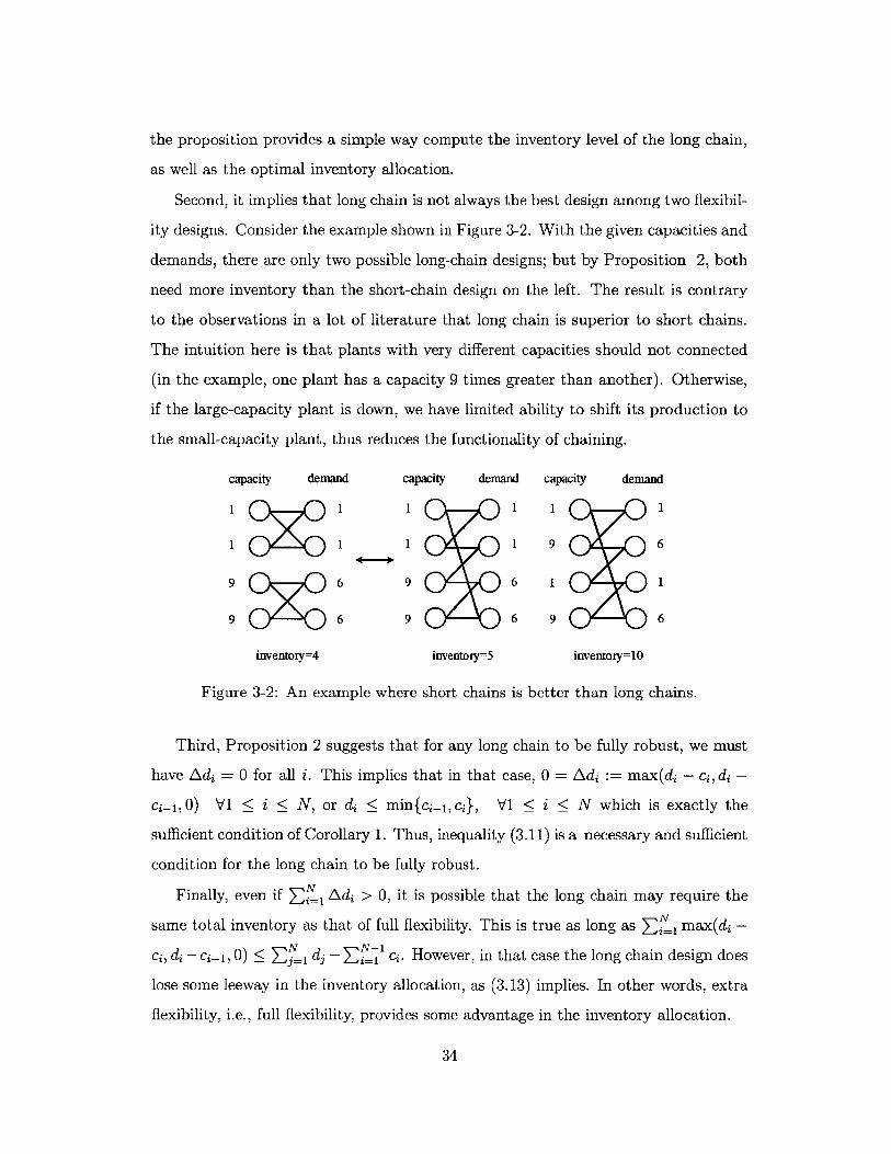
Second, it implies that long chain is not always the best design among two flexibil-

ity designs. Consider the example shown in Figure 3-2. With the given capacities and

demands, there are only two possible long-chain designs; but by Proposition 2, both

need more inventory than the short-chain design on the left. The result is contrary

to the observations in a lot of literature that long chain is superior to short chains.

The intuition here is that plants with very different capacities should not connected

(in the example, one plant has a capacity 9 times greater than another). Otherwise,

if the large-capacity plant is down, we have limited ability to shift its production to

the small-capacity plant, thus reduces the functionality of chaining.

capacity demand capacity demand capacity demand

1 1 1 1 1 1

1 1 1 1 9 6

9 6 9 6 1 1

9X 6 9 6 9 6

inventory=4 inventory=5 inventory=10

Figure 3-2: An example where short chains is better than long chains.

Third, Proposition 2 suggests that for any long chain to be fully robust, we must

have Adi = 0 for all i. This implies that in that case, 0 = Adi := max(di - ci, di -

ci_1,0) VI < i < N, or di < min{cj_1 ,cj}, VI 0, it is possible that the long chain may require the

same total inventory as that of full flexibility. This is true as long as Eil max(di -

ci, di - ci_1 , 0) < EN dj - EN-1 c,. However, in that case the long chain design does

lose some leeway in the inventory allocation, as (3.13) implies. In other words, extra

flexibility, i.e., full flexibility, provides some advantage in the inventory allocation.

34

3.2.1 Design of the Long Chains

Evidently, as we have seen in the example in Figure 3-2, there are many different

ways to form a long chain. Suppose the dedicated network 9 = { (i, i) 11 < i < N} is

a "base network" for which the firm can add process flexibility to form a long chain.

In particular, in the base network, plant i is already matched with product i, and the

objective is to find secondary product that each plant will make.

Note that there are (N - 1)! different long chains which contains 9. Observe that

each long chain can be represented by LC(o-) = 9 U {(o-(i), o(i + 1))11 <i <N}, for

some o such that o-(1), or(2), ... , o-(N - 1) is a permutation of numbers from 1 to N -I

and -(N) = N, o-(N + 1) = o(1). The strategic inventory required to achieve a unit

of TTS clearly depends on the specific long chain. We are interested in the question

of which long chain requires the lowest inventory level.

In particular, we define two special permutations. When a-(i) = i for 1 < i < N-1,

the nodes are connected in increasing order, so we define such permutation as o.+

Similarly, when o-(i) = N - i for 1 <i < N -1, the nodes are connected in decreasing

order, and we define it as o--.

Using the result of Proposition 2, for any fixed o-, the inventory level for LC(o) is

N N-1 N

max{Z d3 - ci, E max{di - ci, d,(i+1) - c,(i), O}}.j=1 i=1 i=1

Therefore, finding the long chain with the lowest inventory requirement is equivalent

to minimizing X:N max{di - c, d,(i+1) - c,(i), 0}.

We start by considering the case where the capacities and demands are matched

in -9, or di = ci, Vi = 1, .. .,n. Thus,

max{di - ci, d.(i+1) - co(i), O} = max{do(i+1) - ca(i), 0}.

Without loss of generality, suppose di < d2 < ... dN. Let t be the index such that

35

a-(t) = 1, then

N N-1

E max{d,(i+1) - cu(i), 0} > E max{d,(i+1) - ca(i), 0}

i=1 i=t

N-1

SZ(do(i+) - d7(j))i=t

= do(N) - do(t)

= dN - d1.

It is easy to check that when - = o+ or o-, the equality is achieved. While LC(o+)

and LC(o-) are the long chains with the lowest inventory level, this level does not

necessarily equal to the level of full flexibility.

The above result motivates a more general analysis for the case when di and ci are

not necessarily equal. Suppose ci 5 C2 ... < cN, d1 < d2 ... < dN, and ci > di for

1 < i < N. The condition essentially states that in the base network 9, demand can

be satisfied when there is no disruption, and the plants with high capacities produce

high volume products. We prove that LC(o+) = 9 U {(i, i + 1)11 di

for 1 < i < N, the inventory level for LC(o.+), associated with a given TTS, is less

than or equal to that of any other long chain design with the same TTS.

We start the proof with two technical lemmas.

Lemma 2. For any o- where o-(1), o-(2), ..., o(N- 1) is a permutation of numbers from

1 to N - I and u(N) = N, u(N + 1) = o-(1),

N T

Zmax{d(i+1 ) - c.(i), 0} maxfd,, - c,, 0},i=1 t=1

where 1 = yo < y1 < y2 < -.. < yT = N.

Proof. Let io be the integer such that o-(io) = 1. For each t > 1 if it_ 1 < N, let

it be the smallest integer satisfying it > it-1 and o-(it) > o-(it_ 1). Such it exists

36

because N is always a candidate. We also have o-(it - 1) < o-(it-1). Otherwise, if

-(it - 1) > -(it_1), index it - 1 will contradict the fact that it is the smallest integer

satisfying the condition.

As sequence it is increasing with t, it will finally end up with an integer T such

that iT = N. Then

N

max{d,(i+1) - c,(i), 0}

(because o-(it - 1) < o-(it_1))

Let yt = o-(it) for 0 < t < T, and we are done.

T

> E max{d,(i,) - c(it- 1), 0}t=1

T

> max{do(it) - c,(it_ ), 0}t=1

El

Lemma 3. Given c1 <; C2 < ... 5 CN, d1 < d2 < ... dN, and ci di for 1 i < N,

b-1

max{db - ca, 0} > E max{dj+1 - c;, 0}

for any positive integers 1 < a 0.

If T = 0, the result trivially holds. If T = 1,

b-1

Emaxfdi+1- Ci, 0} = dj1+1 - cil < db - Ca < max{db - Ca, 01

and if T > 2,

b-1

Z max{dj+1 - ci, 0}

T

= Z(dit+1 - ci,)t=1

T-1

= (diT+1 - CiT) + (dit+1t=2

T-1

(because it_1 + 1 < it)

- cit) + (dj 1+1 - cil)

< (db - ciT_1+1) + Z(dit+1 - ci, 1+1) + (di 1+1 - Ca)t=2

37

T-1

< (db - diT-+1) ± i+ - dit-i+1) ± (dii+1 - Ca)

t=2

= db - Ca-

This completes the proof.

Combining Lemma 2 and Lemma 3, we show that LC(u+) requires the lowest

inventory level among all LC(o-).

Proof of Proposition 3. Fix some permutation o that defines a long chain. By Propo-

sition 2, the inventory needed for LC(o) is equal to

N N-1 N

max{Z d3 - ci, max{d,(i+1) - ca(i), 0}}.j=1 i=1 i=1

On the other hand, the inventory for LC(o.+) is equal to

N

max{Z d -j=1

N-1 N-1

ci, max{di+1 - ci, 0}}.i=:1i=

Thus, it is sufficient to prove that

N-1

max{do(i+1 ) - co(i), 0} > max{di+1 - ci, 0}.i=1i=

By Lemma 2, there exists some positive integer T and a sequence 1 = yo < y1 <

Y2 < ... , < YT = N, such that

T

Z max{do(i+1) - c.(i), 0} > E max{d, - cyti, 0}

(by Lemma 3)

t=1

T yt-1

>2 maxf di+1 - ci, 0}t=1 i=yt-1

N-1

max{di+1 - Ci, 0}.i=1

0

38

N

N

i=1

El

By the proposition, when ci < c2 < ... cN, d1 < d2 < ... < dN, and ci > di for

1 < i < N, the best long chain, LC(o.+), requires

N N-1 N

maxZ d_ - E ci, Zmax(di - ci1, 0). (3.18)j=1 i=1 i=1

units of inventory to achieve one time unit of TTS.

If the condition of Proposition 3 does not hold, our numerical experiments sug-

gest that a rule of thumb is to add flexibility links where capacity and demand are

close to each other. The intuition is that, if the capacity is much larger than the

demand, the exceeding capacity is wasted; if the capacity is much lower than prod-

uct demand, because each product is produced by only two plants, large amount of

strategic inventory is required in case the other plant is disrupted.

While (3.18) is equal to the inventory needed for full flexibility when di - ci_1

is small for 1 < i < n, it can be strictly greater than the inventory needed for full

flexibility in some instances. However, in the next section, we show that there exists

a specific long chain for which adding one degree of flexibility to each of the plant

provides a design that is fully robust.

3.3 Other Sparse Flexibility Designs

In this section, we again consider a system with ci > di for 1 <i < N and di < d2

... < dN. We show that in this setting, there exists a fully robust sparse design where

each plant node is incident to at most 3 arcs.

Proposition 4. In a system with N plants and N products, suppose Ci > di for

1 < i < N and d1 < d2 < ... dN. Let F = LC(--)U {(i, N)|1 < i < N -1}. Then

F is fully robust.

Proof. Fix any Y C {1, 2,.. , N} such that or(Y) G; {1, 2,... , N}. Because 6o({N}) =

{1,2,..., N}, we must have N 0 Y, or Y g {1, - -* , N - 1}. Notice that for any

i E (1, . .. , N - 1}, ci > di, cj+1 > di. Thus, we can apply the same proof as in

39

Corollary 1 and get

Sd < ci - max ci.jEY iES-y(Y) iEF(Y)

Apply Theorem 1, and we have that Proposition 4 holds. l

Proposition 4 further justifies the claim that for any system, when products de-

mands are not volatile, sparse flexibility design is enough for mitigating supply chain

risks.

We note that under some circumstances, full robustness can be achieved by adding

less flexibility than what is described in Proposition 4. Hence, Proposition 4 is not

necessarily the most effective method of adding flexibility to increase supply chain

robustness, but rather a justification of the insight that it is possible to achieve full

robustness with sparse design.

40

Chapter 4

Uncertain Demand

In this chapter, we relax the assumption that products demand is deterministic.

Instead, we assume all possible demand values belong to an uncertainty set, and

the exact value is realized after the disruption happens. The firm is able to change

the production level after disruption, but inventory decisions are made before demand

is realized. The objective is to maximize the TTS in the worst case. We choose a

worst-case analysis for demand uncertainty to make it consistent with the definition

of TTS, which itself is a worst-case risk measurement.

Our interest in this chapter is to understand the effectiveness of flexibility under

demands with different levels of variations. Throughout the chapter, we will consider

uncertainty set U, with the form

M

U {(di, d. ) | dj = D,l dj < u}.j=1

We also suppose 1 = (1 - a)D/M and u = (1 + a)D/M, where the parameter a

indicates the level of uncertainty. We note that while the uncertainty sets under

consideration are highly stylized, it contains enough freedom that allows us to study

the effectiveness of flexibility with different levels of demands uncertainties. A more

general form of uncertainty sets would lead to unnecessarily complex analysis or even

intractable mathematical models.

41

4.1 Uncertain Demand Time-to-Survive Model

Following the notation in Chapter 2, the problem can be formulated as follows, which

is referred to as the Uncertainty Strategic Inventory Problem (Problem U-SI) here-

after.

M

Problem U-SI: s* =min max min ssj dj x n)E

Sj=1

s.t. dj- X 2 s8,i: (i)EF

X ) ci, V1 <

j: (ij)EF

X 0, V1 <j: (n,j)EF

M

Zd = D,j=1

l di < u, s,4) > 0.3' z

(4.1)

V1 < n < N,1 j < M

i,n < N

n < N

To avoid unnecessary complication, we suppose that the number of products M =

2m is even. The result when M = 2m + 1 is odd can be solved similarly, and can be

found in Appendix B. As we did in for the deterministic demand, we will compare

the TTS of full flexibility design and long chain design in the uncertainty case.

4.2 K-Flexibility Designs

In this section, we consider a symmetric K-flexibility design where plant 1 produces

product 1 to product K, plant 2 produces product 2 to product K +1, and in general

plant i produces products i, i + 1, .. , i + K - 1. We assume here again that M = N,

M is an even number, and the capacity of each plant equals to c. Both full flexibility

(K = M) and long chain (K = 2) are special cases of this type of design.

To solve Problem U-SI (4.1) for K-flexibility designs, we first prove the following

lemma.

42

Lemma 4. Suppose for any inventory allocation s = (S1, s2, - - -, SN), the rearranged

allocation o-(s) = (s 2 ,S3 -.. , SN, S1) (stock S2 units of product 1, etc.) achieves the

same TTS for Problem USI, then the optimal TTS can be achieved by allocating R

units of inventory equally among all products.

Proof. If two inventory allocations s = (si, s2, ... ,SN) and s' = (si, s',-- , sN) both

have TTS greater than or equal to one time unit with any demand in the uncertainty

set U, their convex combination (of s and s') also has TTS greater than or equal to

one. This is easy to see from the model of Problem USI (4.1): for any demand in

U, if the production x is feasible for s, and x' is feasible for s', then Ax + (1 - A)x'

is feasible for inventory allocation As + (1 - A)s'. By assumption, if the inventory

allocation s achieves the maximum TTS, so do a(s), a.2 (s), . - - , o.N-1(s). Therefore,

their convex combination s = (s, i,..., s), where E = i si/N, achieves a TTS at

least as good. Therefore, s also achieves the optimal TTS.

The symmetry of K-flexibility designs certainly satisfies Lemma 4, so we can

assume sj = s for all product j. We can there characterize the inventory level for

K-flexibility designs under uncertain demand.

Proposition 5. Suppose K < N/2. An equal inventory allocation s = (s, s,... , s) in

a K-flexibility design will achieve a unit time of TTS for all demands in uncertainty

set U if and only if it does so for such a demand instance: di = l,Vi = 1,..., N/2,

di = u,Vi = N/2 + 1, ..., N.

Proof. Since U is polyhedral, Problem USI (4.1) suggests that s can achieve TTS of

one for all demands in U if it can do so for all vertices of U. A vertex of U has the

following characterization: Half of the products have upper bound demand u and the

rest have lower bound demand 1. So we only need to focus on these demand instances.

For a given demand and inventory vectors, inequality (3.9) tells us that the system

achieves a unit TTS if and only for any subset of plants X and the products they

43

produce 6(X), it holds

N

ci -max ci + (dj - s)+ > Z(dj - sy)+. (4.2)igx jEb(X) j=1

In this case, Ci = C, Si = s, dj = u or 1.

We start by identifying the range of the uncertainty level, a, where the total

inventory needed in K-Flexibility equals to D - (N - 1)c, the inventory level for

full flexibility in the deterministic case. Because K-flexibility is a superset of the

long chain and a subset of full flexibility, c/D < a < (N - 1)c/D. In this range,

u - s > c> 1 - s > 0, so the condition (4.2) can be simplified as

S(d - s) ci = c|X.jE3(X) iEX

The minimum of f(X) = Zje6(x) (dj - s) - cIX| is reached when 6(X) only contains

products with demand 1. Otherwise, if there is a product j E 6(X) with d = u, we

can delete the plant in X that produces j to reduce the value f(X). So we can let

f(X) = (1 - s)|6(X)| - cIXI.

Observe that by definition of K-Flexibility, lo(X) I > X| + K - 1, and equality

holds when plants in X are clustered, that is plants indices in X are consecutive.

Also, because 1 - s < c, the minimum of f(X) is reached when 6(X) contains all

products with demand 1. Hence, the "worst" demand happens when N/2 consecutive

products have demand 1. The inequality in this case is a < (2K - 3)c/D.

If a > (2K - 3)c/D, let Aa = a - (2K - 3)c/D. The inventory level s =

D/N - (N - 1)c/N + AaD/N = (1+ a)D/N - (N + 2K - 4)c/N is enough to achieve

a unit TTS, because it offsets any demand amount that exceeds the threshold. Thus,

(1 + a)D/N - (N + 2K - 4)c/N is an upper bound on the amount of inventory

required for a unit TTS. To see that this is also as lower bound, let 6(X) be the N/2

consecutive products with demand 1 in condition (4.2). We have

s > (1 + a)D/N - (N + 2K - 4)c/N.

44

So the proof is complete.

4.3 Results and Comparisons

Proposition 5 implies that the strategic inventory for a K-flexibility design (K < N/2)

is

Strategic Inventory D-C if 0 a < (2K - 3)c/D,

(1+ a)D - (N + 2K - 4)c if (2K - 3)c/D < a < 1.

(4.3)

Recall that D - C = j dj - E ci is the total inventory required for K-

flexibility when demand is deterministic, which is consistent with the solution when

a = 0. As a increases, the level of demand uncertainty increases. (4.3) suggests

that for low degree of uncertainty, i.e., 0 < a < (2K - 3)c/D, the inventory level is

unchanged. However, as the level of uncertainty increases beyond a certain value, a

K-flexible system needs more inventory to achieve a unit of TTS.

Example 1: The Long Chain Design.

By equation (4.3), for long chain designs, the inventory needed is given by

SI= D-C if 0 < a < c/D, (4.4)(1+a)D-Nc ifc/D<a 1.

Example 2: The Full Flexibility Design.

When K > N/2 + 1 (including full flexibility), it is easy to check that equally

allocating the total inventory of (N/2 +1)-flexibility design is feasible for K-flexibility

to achieve a unit TTS. Therefore, the total inventory needed for K-flexibility design

(K > N/2 + 1) to achieve a unit of TTS is the same as that of full flexibility (given

by (4.5)).

{ )DD-C if 0 < a < C/D, (4.5)(1 + a)D - 2C if C/D < a < 1.

45

0

To summarize, the result is shown in Figure 4-1.

Long Chain

Inventory K-Flexibility

Full Flexibility

0 c;D (N-1)c/D 1 a

(2K-3)c/D

Figure 4-1: Inventory needed to achieve 1 time unit of TTS with uncertain demand.

We can now compare the strategic inventory needed for full flexibility with that

of the long chain, for a system with n plants having identical production capacity

c. When the uncertainty level a, is small, i.e., 0 < a c/D, there is no difference

between the two systems, and in fact the inventory level is the same as in the deter-

ministic one. As a increases above c/D, the performance of the long chain decreases

and long chain needs more inventory than full flexibility.

Note that c is the capacity of an individual plant and C is the total capacity

of all but one plants, so the threshold c/D for long chain is much smaller than

C/D = (n - 1)c/D of full flexibility, as Figure 4-1 shows. In addition, as the number

of products increases, c/D would decrease but C/D would increase, so the difference

between long chain and full flexibility becomes even larger.

The result shows that with high uncertainty in demand, the long chain design

may not be enough and the firm may need to invest in additional flexibility to keep

inventory levels low. For example, when K = 3, the threshold for 3-flexibility design

is 3c/D, a substantial improvement over c/D, the threshold of the long chain.

One way to explain this improvement achieved by 3-Flexibility is that the chaining

strategy in the long chain design is very effective in satisfying uncertain demand (see

Jordan and Graves, 1995). However, a disruption breaks the chain, and hence reduces

46

the ability to satisfy uncertain demand. On the other hand, a 3-flexibility design

retains the chaining structure even if one plant is down, and hence it has a much

better performance than the long chain design.

47

Chapter 5

Assembly Networks

Motivated by the Toyota case in the introduction part of Chapter 1, we include sup-

pliers into the TTS model. Sometimes the company cannot afford to hold inventory of

expensive final products. Therefore, it is worthwhile to apply TTS to an assemble-

to-order manufacturing system, where suppliers can stock inventory of components

(e.g., auto components), but assembly plants cannot stock inventory of final products

(e.g., automobiles).

5.1 The Assembly Network Model

To be specific, we consider a two-stage manufacturing network shown in Figure 5-

1. There are N suppliers, represented by squares on the left-hand side, producting

M components, represented by circles. The components are then made into L final

products, represented by triangles, by assembly plants. The manufacturer can stock

inventory for components, but cannot do it for final products. Also, suppliers are

subject to disruptions, where any of them can be down. Because assembly plants do

not hold inventory, we assume they will not be disrupted. (Or, more realistically, we

can assume the company has extra capacity for assembly plants, so that even if one

of them is down, normal production can resume; there we dismiss the cases where

assembly plants are disrupted.) The objective is to allocate inventory of components

to maximize the TTS of final products.

49

Supplier Component

Final Product

Figure 5-1: An illustration of assembly system.

For convenience, we introduce bill of materials (BOM), which is represented by

a matrix A. An element of A, ajk, means that final product k requires ajk units

of components j. Suppose that vector d is the demand of final products, and that

vector y is the corresponding demand of components, then we immediately know that

y = Ad.

Suppose U is the uncertainty set for final product demands. The Assembly-

Network Strategic Inventory Problem (Problem A-SI) can be formulated as follows.

Problem A-SI :M

s*= min s (5.1)j=1

s.t. aj d(w) - x (cj) < sj, V1 < n < N, 1 < j < M, d(w) E Ui: (ij)E F

S 4)(w)<cj, V1<i,n N,d(w)EUj: (i )E Y

5 a{)(w)= 0, V1 < n < N, d(w) E Uj: (n,j)EF

sj, z (W) > 0.

In the above problem, d(w) is an instance in the demand uncertainty set U; 47z (w) is

corresponding production element, representing the units of component j produced

50

by supplier i when plant n is disrupted. aT is the jth row of matrix A, representing

the units of jth components needed for each final product.

It is immediately clear that when the demand is deterministic, Problem A-SI

reduces to Problem SI discussed in Chapter 3: if demand of final products is d, one

only need to consider a one-stage network including only suppliers and components,

where the demand of components is given by y = Ad. Therefore, we shall focus on

cases where demand is uncertain.

5.2 Uncertainty Set for Components

In Chapter 4, we assume that U is a polytope. Since U is a polytope, Problem U-SI

(4.1) suggests that strategic inventory s can achieve TTS of one for all demands in

U if it can do so for all vertices of U. Indeed, given inventory level s, if demand d

can be satisfied by feasible production vector x, demand d can be satisfied by R, then

ad + (1 - a)d can be satisfied by ax + (1 - a)R, which is also feasible. Therefore,

for Problem U-SI, one only need to focus on the vertices of U.

The result can be extended to Problem A-SI (5.1). Suppose the demand of final

products d lies in a bounded polyhedral uncertainty set U. The bill of materials is

defined by a matrix A, so that the demand of components is y = Ad. All possible

demands of components lie in the set

y = {y | y = Ad,d E U},

is also a bounded polyhedron (a proof is given by Fourier-Motzkin elimination). By

the same argument as before, one only need to focus on the vertices of Y.

Note that if d is a vertex of U, Ad is not necessarily a vertex of Y. However, the

following result assures that focusing on the vertices of U is enough.

Proposition 6. If y is a vertex of Y, there exists a vertex d of U such that y = Ad.

Proof. Suppose that {d(k) I k = 1, ... , K} is the set of vertices of U. Let y(k) =

Ad(k), Vk = 1,... , K. If there exists k such that y = y(k), the proof is complete. If

51

not, we can express y as y = Ad, and d = aid(1) + a 2d(2) + -- - + aKd(K), where

k_1 ak = 1, 0 < ak 1, Vk, and at least one a(k) E (0, 1). This implies that

y = A(aid(1)+ a 2 d(2)+ - - -+ aKd(K)) = a1y(1) + a 2y(2)+ - - -+ aKy(K) is a convex

combination of y(K), which contradicts to the fact that y is a vertex of Y. O

By Proposition 6, if all vertices of final product uncertainty set U are known, the

inventory level to achieve a unit of TTS of the assembly network under uncertain

demand can be calculated as follows.

M

s= mn Si (5.2)

s.t. a d(k) - x(k) sj, V1 < n < N, 1 j < M, 1 < k < Ki: (ij)EF

x,7)(k) < ci, V1 < _, n < N, 1 < k < Kj: (ij) EF

5 (n)(k)=O, V_n N,1 k<Kj: (n,j)ET

sj 7 x7 (k) > 0.

In the above problem, {d(k) | k = 1,... , K} is the set of vertices of U, and aT is

the jth row of matrix A, representing the number of jth components needed for each

final product.

5.3 Total Amount of Strategic Inventory

It is evident that in Problem A-SI, allocating strategic inventory equally among all

components is often not optimal. Therefore, Problem A-SI is much harder to solve

than Problem U-SI discussed in Chapter 4. Despite this difficulty, TTS of assembly

network can be characterized analytically when there are only two final products.

Suppose there are two final products with demand that belongs to the uncertainty

set

U={(di, d2 ) I (1 - a)J < di < (1+ a)d,Vi = 1, 2; di + d2 = 2d}.

52

There are only two vertices in U: d(1) = ((1- a)j, (1+a)j) and d(2) = ((1+a)j, (1-

a)j). It is easy to see that for the d(1), the associated demand for component i is

yi = (an+ai2)j-a(ani-ai2)jand similarly for d(2), yi = (ail+ai2)+a(ani-ai 2 )d. We

denote by gj = (ai +ai2 ) jthe average demand for component i. Let Ayi = (ai1 - a 2 )d

and hence

yi = gi - ayi, y = Yi + aAyi,

which implies that Ayi can be viewed as demand variation.

If component i is a standard component, that is, a component used by multiple

products, see for example the third component in Figure 5-1, fAyil is likely to be

small because of the risk pooling effect. On the other hand, if component i is used

by only one product, IAyil is likely to be large.

For the following two propositions, we suppose the number of suppliers equals the

number of components, i.e., M = N. As usual, C = ci - maxN=, ci is the worst

case total suppliers capacity under disruption.

Proposition 7. Suppose suppliers are fully flexible, i.e., each supplier can produce

all the components. Then the strategic inventory required to achieve one time unit of

TTS is given by

E { i + i if a < aFF,SI=- Ai C (5.3)

iNl i + aFF Zft 1 Ayi - 0+ (a - aFF) 1 Ayi if a > FF

for some constant a FF-

Proof. For a full flexibility network, the maximum total demand is given by ENli ±a N Ayi . Therefore, the total inventory needed is at least

N N

> i+ a EAyI - C, (5.4)i=1 i=1

where C = Eci - maxf=i1 ci. With the total inventory given by equation 5.4, the

53

minimum total demand is automatically satisfied if

N N N N

EZ9i -aZIiyiI> E i -aZAyij - C,i=1 i= i=1 =1

orN N

a < C/(E Ayi - IEAy I).i=1 i=1

Beyond this threshold, the inventory needed increases at slope Ej 1Ayjl with a.

But this part may not exist, e.g., when E i lAyil = 1i Ay; .

Proposition 8. Suppose each supplier can produce two components, and the process

flexibility of suppliers forms a 2-chain design. Then the strategic inventory required

to achieve one time unit of TTS for a 2-chain two-product assembly network is given

by

SI= E{ 1 i+aEAy - C, if C < aLc, (5.5)1N max {gj + a|Ayjl - ci, gi + alAyjl - ci_1, 0}, i ti= if e> aLc

for some constant aLC < aFF-

Proof. By Proposition 2, the network has one unit of TTS (under uncertainty) if and

only if

N N

E(yi - SO)+ _ C, E(yi - si)+ < C, (5.6)i=1 i=1

(yi - si)+ < ci, (yi - si)+ < ci, (5.7)

(yi - si)+ < ci_ 1, (y - s) 5 ci- 1. (5.8)

Equations (5.7) and (5.8) are equivalent to the following condition

si > maxt{Vj + venAY - c, e + ae 2Ay - ci_1, 0}soVi.

Equation (5.6) implies that inventory needed for the 2-chain is at least that of full

54

flexibility, which is given by equation (5.3), i.e.,

N N N

EZsi Zi cdZAyil - C,i=1 i=1 i=1

which is an lower bound provided by the inventory of full flexibility design. E

In Figure 5-2 we apply the two propositions to compare strategic inventory levels

in full flexibility and 2-chain designs for a two-product assembly system.

Long Chain

Inventory

Full Flexibility

0 1 a

Figure 5-2: Illustration of assembly system

The steeper slope in this Figure equals to EZ A yi | while the flatter slope equals

to | EN AyiI. Again, the figure is similar to Figure 4-1, implying that a 2-chain

design does not provide enough flexibility when demand has high uncertainty.

According to Figure 5-2, to reduce strategic inventory for a 2-chain assembly

network, it is more important to reduce Ei 1 |Ayil. As observed in the beginning

of this subsection, |Ayil represents risk pooling of component i, implying that if this

component is used in multiple products, |Ayil is likely to be small. Therefore, for a

2-chain design, one way to reduce strategic inventory is to standardize components

so that they can be used in many final products.

To reduce strategic inventory for a full flexibility assembly network, it is more

important to reduce I Ayi (rather than Ei 1 JAyil). In this case, it is less

important to standardize components since positive and negative Ayi's just cancel

each other out.

55

To sum up these observations, process flexibility and product design flexibil-

ity (e.g., the ability for a component to be used in multiple products) are substitutes

to each other. A network with low degree of process flexibility (e.g., dedicated or

2-chain designs) needs high level of product design flexibility (e.g., standard com-

ponents) to reduce strategic inventory. By contrast, a network with high degree of

process flexibility may need little strategic inventory even with low level of product

design flexibility.

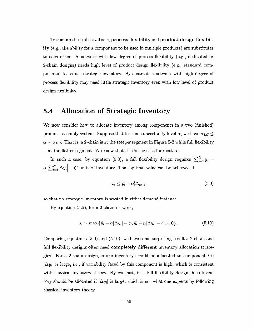
5.4 Allocation of Strategic Inventory

We now consider how to allocate inventory among components in a two (finished)

product assembly system. Suppose that for some uncertainty level a!, we have cLC <

af < aFF. That is, a 2-chain is at the steeper segment in Figure 5-2 while full flexibility

is at the flatter segment. We know that this is the case for most cf.

In such a case, by equation (5.3), a full flexibility design requires E N +

a N ays - C units of inventory. That optimal value can be achieved if

Si < g - aIAyil, (5.9)

so that no strategic inventory is wasted in either demand instance.

By equation (5.5), for a 2-chain network,

si = max{± + alAyil - ci, gj + alAyjI - ci_1, 0}. (5.10)

Comparing equations (5.9) and (5.10), we have some surprising results: 2-chain and

full flexibility designs often need completely different inventory allocation strate-

gies. For a 2-chain design, more inventory should be allocated to component i if

IAyil is large, i.e., if variability faced by this component is high, which is consistent

with classical inventory theory. By contrast, in a full flexibility design, less inven-

tory should be allocated if |Ayil is large, which is not what one expects by following

classical inventory theory.

56

The above counter-intuitive observation can be explained in the following way. In

a 2-chain design, much like in a dedicated network, there is limited capacity for each

component and as a result inventory is used to mitigate against demand variability.

Hence more inventory is required for components facing high variability. By contrast,

in full (or high degree) flexibility design, the system has enough capacity to hedge

against demand variability and hence the concern is to make sure the system does

not have too much inventory. Thus, in this case, it is appropriate to stock more

strategic inventory for products with stable demand. This observation is confirmed

by numerical studies in Chapter 6.

57

Chapter 6

Stochastic Demand

In many cases, firms cannot predict disruptions on the supply side, but they are able

to estimate the distribution of product demand using historical data. Thus, in this

section, we consider the TTS model, when products demands are stochastic and their

distributions are known. The purpose for considering the stochastic demand setting

is twofold: First, in the stochastic model we are able to remove the restrictions in

Chapter 4 where capacities of different plants are equal and demands of different

products have the same range; Second, we would like to evaluate the TTS of different

flexibility structures in the stochastic demand model, and find out whether the results

in Chapter 4 and 5 still agree with the results under stochastic demand model.

6.1 Stochastic Demand Model

Suppose demands for different products are independently distributed. Demand

of product j is a random variable Dj drawn from a distribution on the interval

[(1 - a)dj, (1 + a)d], where dj is the expectation of Dj, and the distribution is

symmetric around dj. Thus, following the notation in Chapter 4, a is proportional

to the coefficient of variation of product demand.

The objective of the firm is to maximize the expected TTS. However, it is possible

that for some low demand instances, even if one of the plants fails, the remaining

capacity is still greater than demand, so that the TTS becomes infinity. To avoid this

59

difficulty, we consider the case where the firm sets a target TTS. A situation where

the actual TTS falls below the target is considered unfavorable. Suppose the actual

TTS is t (a random variable since demand is random), and the target being T. We

assume that the firm is maximizing E[t A T], where t A T = min{t, T}.

The sequence of decisions is similar to the uncertainty model of Chapter 4. The

firm first decides the amount of strategic inventory for each product, according to

the given demand distribution. Once a disruption happens, realized demands are

observed, and the firm decides the production level at each plant.

In sum, the problem can be formulated as a two-stage stochastic program as

follows.

t* = max E[tw] (6.1)

M

s.t. Z rj < R,j=1

rj;O0, Vj=1,...,M.

where the second stage problem is

tw =max t (6.2)

s.t. t < _ V1<n<N, 1j<M

i: (i,j)EF

S k~ci, V1 in<5Nj: (i,j)EF

4)" 0, V1 < n < Nj: (n,j)EF

t <T,

> 0.

Here, dj' is the demand of product j, which is realized at the second stage. We

also rewrite the objective function E[t AT] by adding a constraint t < T in the second

stage problem.

60

Finally, it is easy to verify that the second stage problem (6.2) can be reformulated

as a linear program, by introducing new variables y7) := t - x . This fact would be

helpful in the numerical tests below.

6.2 Numerical Examples for One-Stage Networks

In the following examples, we assume the firm produces five products from five plants.

Plants capacities are chosen uniformly in [0.8,1.2]. The expectations of demands are

chosen uniformly in [0.7, 1.1]. For each Product j, the demand D is assumed to have

independent discrete uniform distribution between [(1 - a)dj, (1 + a)dj], where dj is

the expectation of Dj, and a is a constant between [0, 1], measuring the variation of

demands.

In the first example, we compare the expected TTS of four different flexibility

designs under different demand variation levels. The four structures are the long

chain; the long chain with additional flexibility (defined in Section 3.3), we refer to

this design as long chain additional; 3-flexibility (defined in Section 4.2), and full

flexibility.

To evaluate the different designs, we start with a given level of inventory R in (6.1),

and determine the expected TTS of each of the four designs. In our computational

tests, we choose R as the total inventory of the long chain required to achieve one

unit time of TTS in the determinstic case. In this example, it is also the inventory

for full flexibility in the deterministic case, so all structures have a TTS of one when

a = 0. Finally, we set the target TTS in (6.2) to be 1.

The result is shown in Figure 6-1. As expected, when the variation of demand

increases, the performance of long chain drops quickly compared to full flexibility,

indicating the need of extra flexibility. It may be surprising, though, that the 3-

flexibility structure performs exceptionally well. The reason is that there are only

five plants in this case, so 3-flexibility is close to full flexibility, that is, 5-flexibility.

Of course, when the number of plants increases, the gap (in expected TTS) be-

tween 3-flexibility and full flexibility is expected to increase. For example, consider

61

Figure 6-2 where we focus on a model with ten plants and ten products. As demand

variation increases, the expected TTS of 3-flexibility drops quickly compared to full

flexibility, but it still has significant advantage over the long chain. These examples

of the stochastic demand model support our conclusion in Section 4 that extra flex-

ibility is needed to protect the system from disruptions when the level of demand

uncertainty is high.

0.9 Full flexibility

0.8-

Ci)

0.7-0

3-Flexibility0.6 -

W Long chain (additional)

0.5-

0.4 Long chain-*

0.3 a I II I I aI0 0.1 0.2 0.3 0.4 0.5 0.6 0.7 0.8 0.9 1

Demand Variation a

Figure 6-1: Expected TTS against demand variations with 5 plants.

0 0.1 0.2 0.3 0.4 0.5 0.6Coefficient of Variation

0.7 0.8 0.9

Figure 6-2: Expected TTS against demand variations with 10 plants.

62

Ci)

*00

0

w

Finally, instead of assuming that total strategic inventory is fixed, we can also

consider a case where the firm needs to decide the amount of strategic inventory so

that the expected TTS reaches a predetermined level. Figure 6-3 shows the results

for the five plants, five products model. It shows the amount of inventory needed such

that the expected TTS is 95% of the target TTS (of one unit time). It is insightful to

compare these results with the results of Figure 4-1 for the uncertain demand model.

Again, the figure shows that the inventory needed for the long chain rises more quickly

than that of full flexibility as demand variability increases.

4.5

4-

z 3.5- Long Chain

1.5 -

Full Flexibility0.5

0 0.1 0.2 0.3 0.4 0.5 0.6 0.7 0.8 0.9 1Dernand Variable a

Figure 6-3: Inventory against demand variations.

6.3 Numerical Example for Assembly Networks

We consider an assembly network described in Chapter 5. In the network, there are

eight suppliers producing eight different components, which are assembled into three

final products. Two of the eight components are standard components, that is, com-

ponents used in all three final products. Each of the remaining components is used

in a single product-these are referred to as non-standard components. Final prod-

ucts expected demand and demand distribution as well as the suppliers production

capacities are chosen in the same way as in the previous subsection.

63

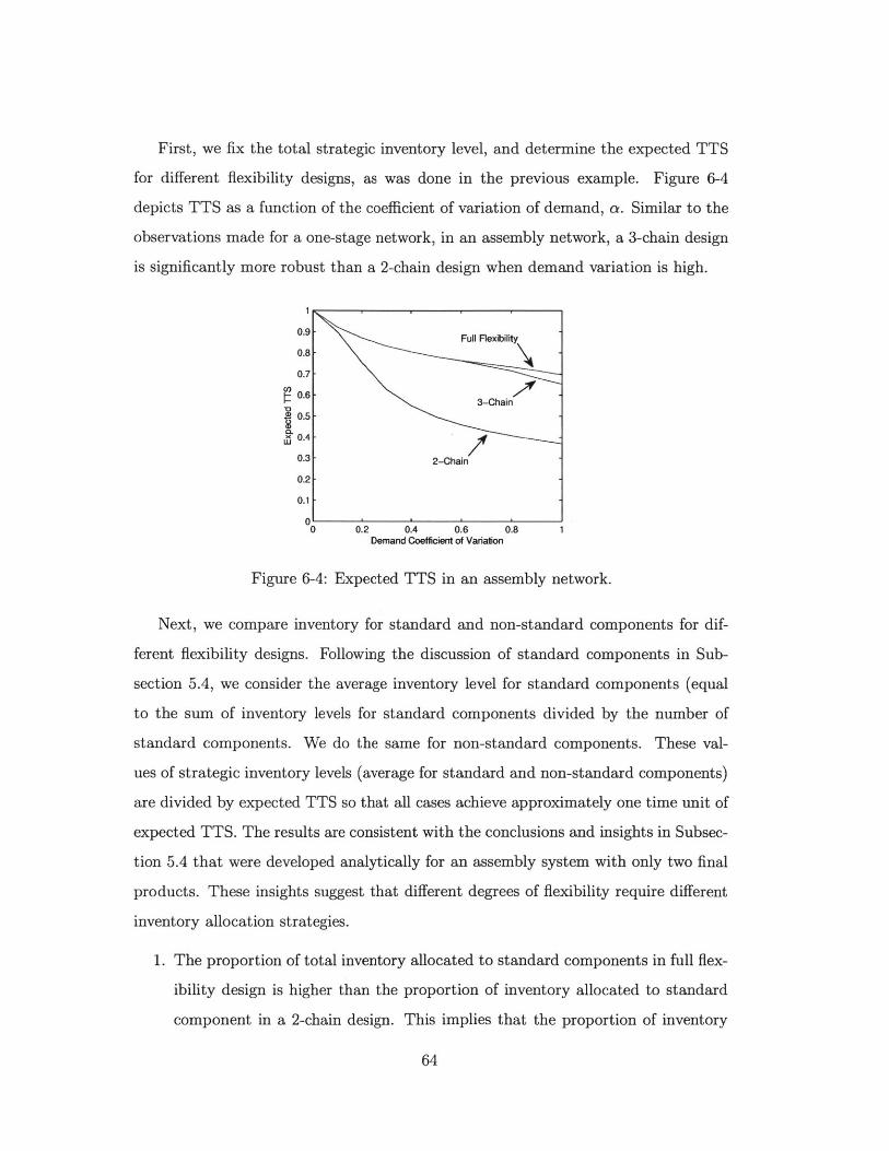
First, we fix the total strategic inventory level, and determine the expected TTS

for different flexibility designs, as was done in the previous example. Figure 6-4

depicts TTS as a function of the coefficient of variation of demand, a. Similar to the

observations made for a one-stage network, in an assembly network, a 3-chain design

is significantly more robust than a 2-chain design when demand variation is high.

0.9 - Full Flexibility0.8 -

-Fl leii0.7

000.6 3-Chain

0.5 --

0.4-

U0.3 - 2-Chain/

0.2

0.1 --

00 0.2 0.4 0.6 0.8 1Demand Coefficient of Variation

Figure 6-4: Expected TTS in an assembly network.

Next, we compare inventory for standard and non-standard components for dif-

ferent flexibility designs. Following the discussion of standard components in Sub-

section 5.4, we consider the average inventory level for standard components (equal

to the sum of inventory levels for standard components divided by the number of

standard components. We do the same for non-standard components. These val-

ues of strategic inventory levels (average for standard and non-standard components)

are divided by expected TTS so that all cases achieve approximately one time unit of

expected TTS. The results are consistent with the conclusions and insights in Subsec-

tion 5.4 that were developed analytically for an assembly system with only two final

products. These insights suggest that different degrees of flexibility require different

inventory allocation strategies.

1. The proportion of total inventory allocated to standard components in full flex-

ibility design is higher than the proportion of inventory allocated to standard

component in a 2-chain design. This implies that the proportion of inventory

64

allocated to non-standard components is higher in a 2-chain design than that

of full flexibility.

2. As demand variation increases, more inventory is needed to achieve one time

unit of TTS. For a 2-chain design, the increment of inventory is mainly allo-

cated to non-standard components. However, for a full-flexibility design, the

increment is allocated to standard components. In this particular example, we

even observe a decrease in inventory level for non-standard components when

the demand variation increases.

3. The inventory level of a 3-chain design falls between a 2-chain design and a full

flexibility design for both standard and non-standard components. In addition,

for non-standard components, 3-chain requires almost the same inventory level

as full flexibility design, but a 2-chain design requires much more inventory.

0.5- 0.5 2-Chain

Full flexibility

3 0.4- 0.4-0 3-Chain

T0.3 A(0.3 3-Chain

0 0.2 - 0.2 -... --- _-

0.1 2-Chain 0.1Full flexibility

0 ' '0 0.2 0.4 0.6 0.8 1 0 0.2 0.4 0.6 0.8 1

Demand Coefficient of Variation Demand Coefficient of Variation

Figure 6-5: The average inventory levels Figure 6-6: The average inventory levelsfor standard components. for non-standard components.

65

Chapter 7

Conclusions

In this thesis, we present the concept of Time-to-Survive (TTS), a metric that we

apply to measure supply chain robustness. TTS is defined as the longest time that

(product or component) demand is guaranteed to be satisfied independent of which

plant is disrupted. We consider two well-studied supply chain strategies, process

flexibility and strategic inventory, that can be applied to increase TTS. Our goal is to

understand the impact of process flexibility and strategic inventory on TTS, including

the relationship between the degree of flexibility and the total amount of strategic

inventory.

To develop insights on the impact of process flexibility and strategic inventory on

TTS, we first consider the case where demand is deterministic. In this case, we show

that given a fixed inventory level and a flexibility design, TTS can be calculated by

solving a linear program. This implies that TTS increases linearly with total inventory

level, but the rate of increase depends on the given flexibility design. We then proceed

to study the inventory required to achieve a fixed TTS for different flexibility designs,

and provide two insights. First, a full flexibility design needs significantly less strategic

inventory than a system with no flexibility, and in addition, it enables a great amount

of freedom in inventory placement. Second, when product demands are equal to each

other than a 2-chain flexibility design is as effective as full flexibility. On the other

hand, when product demands vary significantly, a 2-chain flexibility design may not

be an effective one. However, a little more flexibility, where the degree of each plant

67

note is no more than three, is as effective as full flexibility.

Next, we model uncertainties in product demands using an uncertainty set, and

study the level of inventory required to achieve a fixed TTS for all demand instances

in the uncertainty set. Interestingly, we find that when there is uncertainties in the

demand, there is a big gap between the inventory needed for a 2-chain design and

that of full flexibility. However, the amount of strategic inventory decreases when

a 2-chain flexibility design is replaced by a 3-chain flexibility design. In particular,

a 3-chain design achieves the same robustness as full flexibility under a much larger

range of uncertainty level.

We then extend the TTS model to an assembly system. We consider an OEM

which applies an assemble-to-order strategy and does not hold inventory for final

products, but can ask its suppliers to stock inventory for components. By consid-

ering an assembly system with two final products, we make a few surprising obser-

vations. First, our result suggests that the degree of process flexibility effects the

need for standard components. When the degree of process flexibility is low, as in

dedicated or 2-chain designs, it is important to have standard components to re-

duce strategic inventory. However, standard components are less critical in reducing

inventory under high degree of flexibility. Second, our result suggests that having

flexibility can greatly affect the allocation of strategic inventory between the different

components. In particular, under the dedicated or 2-chain flexibility designs, more

inventories should be allocated to components with high demand volatility, i.e., the

non-standard components, which is consistent with the classical inventory theory.

However, for full flexibility design, more inventory should be allocated to components

with low demand volatility, such as standard components. This dichotomy further

explains why a 2-chain design may not be a very robust process flexibility strategy,

as it displays behaviors similar to a dedicated design than to a full flexibility design.

Finally, to ensure that these findings are not restricted to worst-case demand, we

performed a numerical study to compute the expected TTS of flexibility designs when

demand is stochastic, and find that the simulation results agree with the theoretical

findings.

68

Appendix A

A More General TTS Framework

Suppose the survival time is divided into K periods. The length of period 1 < k < K

is t(k). No matter which plant is disrupted, during period k, the company wants to

satisfy a demand rate of dj(k) for product j. Suppose xz )(k) is the production rate

of product j in plant i during period k when plant n is down. Other assumptions and

notations are the same as in Chapter 2. It is easy to see that product-specific TTS is

a special case of this problem setting.

With some modification of Problem SI, the problem can be formulated as the

following LP.

General TTS:

M

*= min s3 (A.1)

s.t. Et (k) (dj (k) - x7)(k)) < sj, V1 5n<5N, 1 5j<5Mk=1 i: (ij)EF

(A.2)

x7)(k) 5cj, V1<i,n<N, 1 < k < K (A.3)j: (ij)EF

> x(k)=O, V1<n <N,,1<k<K (A.4)j: (n,j)EF

sj, x) (k) > 0.

69

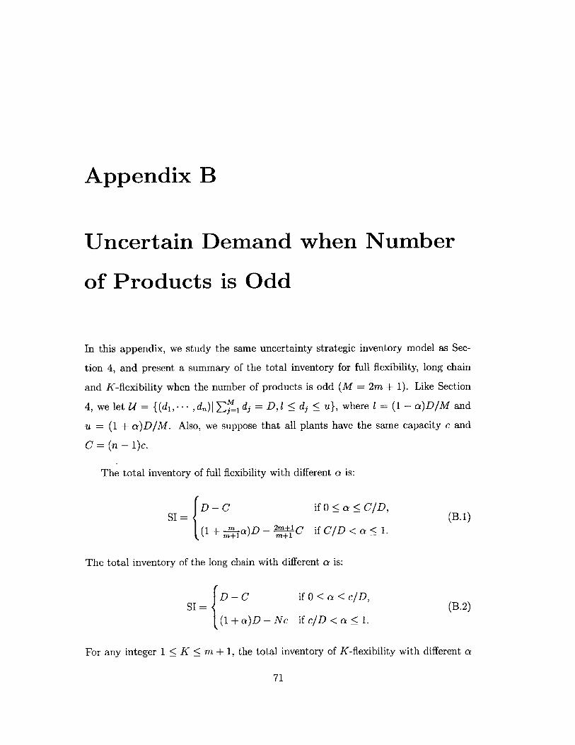
Appendix B

Uncertain Demand when Number

of Products is Odd

In this appendix, we study the same uncertainty strategic inventory model as Sec-

tion 4, and present a summary of the total inventory for full flexibility, long chain

and K-flexibility when the number of products is odd (M = 2m + 1). Like Section

4, we letU = {(di,.- -. )limdj =D,l < dj < u}, where 1 = (1 -a)D/M and

u = (1 + a)D/M. Also, we suppose that all plants have the same capacity c and

C =(n - 1)c.

The total inventory of full flexibility with different a is:

SI= D-C if 0 < a < C/D, (B.1)

(1I+ m a)D - 2m1C if C/D < a < 1

The total inventory of the long chain with different a is:

SI D-C if 0 < a < c/D, (B.2)(1+a)D-Nc ifc/D<a 1.

For any integer 1 < K < m + 1, the total inventory of K-flexibility with different a

71

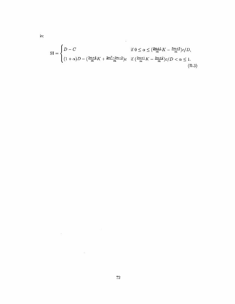
SL=(1 + )D - (2n+1K + 22-3m-2)cm

if 0 < a < (2m+K _ 3m+2 )c/D,

if (2 +1 K -3+2)c/D < a <

(B.3)

72

is:

Bibliography

Arreola-Risa, A. and DeCroix, G. (1998). Inventory management under randomsupply disruptions and partial backorders. Naval Research Logistics, 45(7):687-703.

Bassamboo, A., Randhawa, R. S., and Van Mieghem, J. A. (2010). Optimal flexi-bility configurations in newsvendor networks: Going beyond chaining and pairing.Management Science, 56(8):1285-1303.

Bish, E., Muriel, A., and Biller, S. (2005). Managing flexible capacity in a make-to-order environment. Management Science, 51(2):167-180.

Bish, E. and Wang, Q. (2004). Optimal investment strategies for flexible resources,considering pricing and correlated demands. Operations Research, 52(6):954-964.

Chod, J. and Rudi, N. (2005). Resource flexibility with responsive pricing. OperationsResearch, 53(3):532-548.

Chopra, S., Reinhardt, G., and Mohan, U. (2007). The importance of decoupling re-current and disruption risks in a supply chain. Naval Research Logistics, 54(5):544-555.

Chou, M., Teo, C.-P., and Zheng, H. (2008). Process flexibility: design, evaluation,and applications. Flexible Services and Manufacturing Journal, 20(1):59-94.

Chou, M. C., Chua, G. A., Teo, C.-P., and Zheng, H. (2010). Design for processflexibility: Efficiency of the long chain and sparse structure. Operations Research,58(1):43-58.

Fine, C. H. and Freund, R. M. (1990). Optimal investment in product-flexible man-ufacturing capacity. Management Science, 36(4):449-466.

Goyal, M. and Netessine, S. (2007). Strategic technology choice and capacity invest-ment under demand uncertainty. Management Science, 53(2):192-207.

Goyal, M. and Netessine, S. (2011). Volume flexibility, product flexibility, or both:The role of demand correlation and product substitution. Manufacturing & ServiceOperations Management, 13(2):180-193.

73

Graves, S. C. and Tomlin, B. T. (2003). Process flexibility in supply chains. Man-agement Science, 49:907-919.

Giirler, U. and Parlar, M. (1997). An inventory problem with two randomly availablesuppliers. Operations Research, 45(6):904-918.

Hopp, W. J., Tekin, E., and Van Oyen, M. P. (2004). Benefits of skill chaining in serialproduction lines with cross-trained workers. Management Science, 50(1):83-98.

Huchzermeier, A. and Cohen, M. (1996). Valuing operational flexibility under ex-change rate risk. Operations research, 44(1):100-113.

Iravani, S. M., Van Oyen, M. P., and Sims, K. T. (2005). Structural flexibility: A newperspective on the design of manufacturing and service operations. ManagementScience, 51(2):151-166.

Jordan, W. C. and Graves, S. C. (1995). Principles on the benefits of manufacturingprocess flexibility. Management Science, 41(4):577-594.

Moinzadeh, K. and Aggarwal, P. (1997). Analysis of a production/inventory systemsubject to random disruptions. Management Science, 43(11):1577-1588.

Parlar, M. (1997). Continuous-review inventory problem with random supply inter-ruptions. European Journal of Operational Research, 99(2):366-385.

Parlar, M. and Berkin, D. (1991). Future supply uncertainty in EOQ models. NavalResearch Logistics, 38(1):107-121.

Parlar, M. and Perry, D. (1998). Inventory models of future supply uncertainty withsingle and multiple suppliers. Naval Research Logistics, 43(2):191-210.

Qi, L., Shen, Z., and Snyder, L. (2010). The effect of supply disruptions on supplychain design decisions. Transportation Science, 44(2):274-289.

Schmidt, W. and Simchi-Levi, D. (2012). Nissan motor company: Building opera-tional resiliency. MIT Case Study.

Sethi, A. K. and Sethi, S. P. (1990). Flexibility in manufacturing: A survey. Inter-national Journal of Flexible Manufacturing Systems, 2:289-328.

Simchi-Levi, D. (2010). Operations Rules: Delivering Customer Value through FlexibleOperations. The MIT Press.

Simchi-Levi, D. and Wei, Y. (2012). Understanding the performance of the long chainand sparse designs in process flexibility. Operations Research, 60(5):1125-1141.

Sodhi, M. S. and Tang, C. S. (2012). Strategic approaches for mitigating supplychain risks. In Hillier, F. S., editor, Managing Supply Chain Risk, volume 172of International Series in Operations Research and Management Science, pages95-108. Springer, New York.

74

Song, J.-S. and Zipkin, P. H. (1996). Inventory control with information about supply

conditions. Management Science, 42(10):1409-1419.

Taleb, N. N. (2007). The black swan: The impact of the highly improbable. RandomHouse, New York.

Tang, C. and Tomlin, B. (2008). The power of flexibility for mitigating supply chain

risks. International Journal of Production Economics, 116(1):12-27.

Tomlin, B. (2006). On the value of mitigation and contingency strategies for managing

supply chain disruption risks. Management Science, 52(5):639-657.

Tomlin, B. and Wang, Y. (2005). On the value of mix flexibility and dual sourcingin unreliable newsvendor networks. Manufacturing & Service Operations Manage-

ment, 7(1):37-57.

Tomlin, B. and Wang, Y. (2011). Operational strategies for managing supply chaindisruption risk. In Kouvelis, P., Dong, L., Boyabatli, 0., and Li, R., editors, The

Handbook of Integrated Risk Management in Global Supply Chains, pages 79-101.John Wiley & Sons, Inc.

Van Mieghem, J. (1998). Investment strategies for flexible resources. Management

Science, 44(8):1071-1078.

Van Mieghem, J. A. (2007). Risk mitigation in newsvendor networks: Resourcediversification, flexibility, sharing, and hedging. Management Science, 53(8):1269-1288.

Wallace, R. and Whitt, W. (2005). A staffing algorithm for call centers with skill-based routing. Manufacturing & Service Operations Management, 7(4):276-294.

75

Increasing Supply Chain Robustness through Process ...

Documents

Transcript of Increasing Supply Chain Robustness through Process ...