Working Paper 45/05

INCREASING RETURNS TO SAVINGS AND WEALTH INEQUALITY

Claudio Campanale

Increasing Returns to Savings and Wealth

Inequality∗

Claudio Campanale†

Universidad de Alicante

November 8, 2005

Abstract

In this paper I present an explanation to the fact that in the datawealth is substantially more concentrated than income. Starting fromthe observation that the composition of households’ portfolios changes to-wards a larger share of high-yield assets as the level of net worth increases,I first use data on historical asset returns and portfolio composition bywealth level to construct an empirical return function. I then augment anOverlapping Generation version of the standard neoclassical growth modelwith idiosyncratic labor income risk and missing insurance markets to al-low for returns to savings to be increasing in the level of accumulatedassets. The quantitative properties of the model are examined and showthat an empirically plausible difference between the return faced by poorand wealthy agents is able to generate a substantial increase in wealthinequality compared to the basic model, enough to match the Gini indexand all but the top 1 percentiles of the U.S. distribution of wealth.

Keywords: Wealth inequality, self-insurance, portfolio composition,increasing returns.

∗I wish to thank Per Krusell and Rui Albuquerque for their suggestions during the devel-opment of this project. I also want to thank the editor Victor Rıos-Rull and two anonymousreferees for useful comments. Financial support from the Instituto Valenciano de Investiga-ciones Economicas (IVIE) is gratefully acknowledged. All remaining errors and inconsistenciesare mine.

†Departamento de Fundamentos del Analisis Economico, Universidad de Alicante,03071, Alicante, Spain. Voice: ++34965903614 - Fax: ++34965903898. E-mail: clau-dio@merlin.fae.ua.es

1

1 Introduction

Empirical studies like Hurst, Luoh and Stafford (1998), Dıaz-Gimenez, Quadriniand Rıos-Rull (1997), Budrıa-Rodrıguez et al. (2002) and Wolff (2000) haveshown that earnings, income and wealth are very concentrated, with distribu-tions that are skewed to the right. Of the three variables wealth is by far themost concentrated with a Gini coefficient of 0.78, while the same index for earn-ings and income is 0.63 and 0.57.1 The latter fact is a regularity that is observedover time and across countries as well and has drawn considerable attention inthe quantitative macroeconomic literature.

The basic framework used to explain this fact is the one in Aiyagari (1994)and Huggett (1996) and is based on a stochastic version of the standard neo-classical growth model featuring heterogeneous labor earnings shocks, missinginsurance markets and borrowing constraints. Both models are successful atreproducing qualitatively the empirical evidence. However they are incapableof matching the data quantitatively so that various features, like heterogeneoussubjective discount factors, bequest motives and entrepreneurship have beenused in later work to improve the performance of the basic model.

Both the basic model and the extensions that followed share one key assump-tion about the assets available to the agents to carry out their saving plans. Thisassumption is that there is a single asset in the economy. A consequence is thatall agents, no matter what their income or wealth is, face the same return ontheir investments. This assumption is clearly at odds with reality, since realworld households may choose to hold assets as diverse in terms of return, riskand liquidity as for example housing and stocks or life insurance policies andchecking accounts. To the extent that portfolio composition and returns varysystematically among households, these will have different incentives to saveadding a further potential source of wealth inequality.

The goal of this research is to incorporate this basic feature of households’investment decisions in a stochastic, overlapping generation version of the neo-classical growth model and test whether the existence of increasing returns tosavings is a quantitatively relevant source of wealth inequality. It turns out thatit is: the empirically observed difference in the return faced by poor and wealthyhouseholds in the economy is sufficient to match the Gini index and the shareof almost all percentiles of the U.S. distribution of wealth. This suggests thatso far an important piece of the explanation for the massive concentration ofwealth of real economies has been overlooked.

The model assumes exogenously that returns to saving are increasing in the1The values reported here are taken from Dıaz-Gimenez, Quadrini and Rıos-Rull (1997)

and are based on the 1992 Survey of Consumer Finances.

2

level of wealth without modeling explicitly household portfolio choice; however,this feature of investment opportunities has strong support in the data. Em-pirical research by Bertaut and Starr-Mcluer (2000), Kennickell et al. (2000)and Samwick (2000) clearly shows that the composition of households’ portfo-lios shifts towards larger fractions of high-yield assets, like stocks and businessequity, as the household’s net worth increases. In the paper I first use Surveyof Consumer Finance data on household balance sheets and data on returns ofbroad categories of assets from a variety of sources to give a precise characteriza-tion of the empirical relation between wealth and returns. This exercise revealsthat while the poorest 60 percent of the population faces an average return toits wealth which is close to 1 percent, the top 1 percent invests its wealth atan average return between 4.5 and 6 percent. Then I interpolate the empiricalschedule and use it in a standard model with uninsurable idiosyncratic earn-ings risk that mixes the life-cycle and dynastic framework. The properties ofthe resulting stationary distribution of wealth in the two cases of constant andincreasing returns to savings are compared revealing that when the estimatedreturn function is used a substantial boost to wealth inequality follows closingthe gap between the quantitative prediction of a standard model with constantreturns and the data.

Before moving to the remaining sections of the paper it is important to spenda few words about the interpretation of the positive relation between net worthand portfolio returns that is observed in the data and, based on that evidence, isassumed here. There are two alternative but not mutually exclusive stories thatcan be told to explain this relation. The first is a market imperfection one: itmay be necessary to pay information costs to gain knowledge of the functioningof some asset markets and even then other trading costs are required to actuallyparticipate in those markets. As a consequence only households that haveaccumulated enough wealth may find it attractive to spend the time and moneyneeded to participate in those higher return markets. In support of this viewcome a number of studies like, for example, Paiella (2001) and Vissing-Jørgensen(2001) about the costs of participating in the stock market and by Hong, Kubikand Stein (2001) that find participation to the stock market being positivelyrelated to sociability as a result of the effect that communication with peers hasin lowering information costs. The second story is a behavioral one: according tothis interpretation some agents dislike some assets and decide not to participateeven if this would be optimal based on their risk preferences and on the assetreturn. In support of this possibility the paper cited above by Hong et al.(2001)reports that participation in the stock market in the U.S. is substantially higherfor white than for non-white even after controlling for wealth, income, educationand survey measures of risk tolerance; Guiso, Sapienza and Zingales (2004)

3

reach a similar conclusion with Italian data when comparing participation ratesbetween southern and northern Italians.2

The model presented in this paper is more consistent with the first interpre-tation since it implies a positive feed-back from wealth accumulation to higherreturns and again to further accumulation; moreover it does not assume het-erogeneity in tastes. However it is not in contrast with the behavioral story:by showing that small differences in the return to assets can generate a real-istic concentration of wealth it says that small ex-ante differences in behaviorconcerning portfolio composition may lead to the large observed wealth inequal-ity. Moreover the same positive relation between net worth and the return onsavings assumed in this paper would still be obtained as an ex-post result in abehavioral one.

The rest of the paper is organized as follows. In Section 2 I first review thequantitative literature on wealth inequality. In Section 3 I present an accountof the empirical evidence on portfolio composition at different wealth levels; Ithen construct an empirical schedule that maps net worth into average portfolioreturns. In Section 4 I describe the model, in Section 5 the choice of parametersand in Section 6 the results. Finally Section 7 concludes. Details about theconstruction of the data used in Section 3 and the numerical solution of themodel are given in Appendix A and B respectively.

2 Literature Review

A large number of papers present quantitative models that attempt to explainthe observed wealth distribution. These models share a set of basic assump-tions. First they are populated by agents who receive an exogenous stochasticflow of income. Second, markets are assumed to be incomplete so that it is notpossible to fully insure consumption risk. Finally there is some form of borrow-ing constraints. A notable example of this kind of models is Aiyagari (1994).Agents use accumulated savings in order to buffer negative shocks to incomeand therefore to smooth consumption. While agents are ex-ante homogeneous,ex-post each of them will have experienced a different history of past realizedincomes leading to a different level of accumulated wealth. This model gener-ates a distribution of wealth that is more concentrated than the distribution ofincome, a feature that is qualitatively consistent with the data. However at aquantitative level it grossly under-predicts the observed concentration of wealth.

2The three authors suggest that financial contracts and stocks in particular are trust-intensive contracts. They then exploit variation within Italy of measures of social capital (ofwhich trust is an important element) and show that these are positively related to the use ofchecks, participation in the stock market and the availability of credit.

4

In particular it fails to explain the two tails of the distribution, that is, the verylow level of wealth accumulation by poor agents and the accumulation of hugeestates at the very top of the wealth distribution.

The model in Aiyagari (1994) considers an economy populated by infinitely-lived dynasties in which saving occurs for precautionary reasons. In a relatedpaper Huggett (1996) uses similar assumptions about market structure, butcasts the model in a finite-horizon framework where agents face a realistic life-time profile of earnings and go through the working and retirement stages of life.In this framework saving also occurs to finance retirement consumption. Themodel fares well in terms of matching the Gini index but it obtains this resultby having a large fraction of households with no or even negative wealth whilestill underestimating the large accumulation of assets of the very rich. Moreoverthose with no wealth are entirely concentrated among very young householdsthat face an upward sloping earnings profile and would like to borrow.

Following these two papers various mechanisms have been proposed to im-prove the ability of quantitative models to match the observed concentration ofwealth. These attempts may be broadly classified based on whether their mainfocus is on the left or the right tail of the distribution.

A prototypical example of the first group is the paper by Hubbard, Skinnerand Zeldes (1995). Their model is cast in a finite-horizon framework and featuresboth earnings and health risk. The crucial element is the presence of means-tested government programs that provide a safety net in the form of a floor onconsumption in case of very bad luck. This induces very poor agents not toaccumulate assets at all and rely on public social insurance instead. While notdirectly focused on measuring wealth inequality this model is able to generate asubstantial number of agents with very low or no savings at all without havingthem entirely concentrated among younger agents.

Another institutional feature that has the potential to reconcile the dataon the uneven wealth distribution with the output of quantitative models is aprogressive social security system. This has been used by Domeij and Klein(2002) to account for the large portion of Swedish households with very littlewealth and, coupled with lifetime differences in earning abilities, has also beenproposed by Huggett and Ventura (2000) to explain why low income householdsas a group save a lower fraction of their income than high income householdsdo.

As far as the right tail of the wealth distribution is concerned two mecha-nisms have been proposed so far. Based on the empirical observation, reported inGentry and Hubbard (2000), that entrepreneurs both make a significant share ofvery wealthy households and tend to have higher wealth-income ratios, Quadrini(2000) constructs a model where entrepreneurship is recognized as the critical

5

element to add to a quantitative model to generate a realistic wealth concen-tration. In his model imperfections in financial markets drive a wedge betweenborrowing and lending rates so that the marginal return to saving and investingin the private firm is higher than market returns. Moreover consistent with theempirical evidence, Quadrini assumes that the income flow generated by a busi-ness is more risky than the income of paid employees, increasing precautionarysaving. The model is then able to generate a more realistic wealth concentra-tion and to account for the higher wealth-income ratio and upward mobility ofentrepreneurial households.

The second mechanism exploits intergenerational links in the form of altru-ism and correlation between the earning abilities of successive members of afamily. Castaneda et al. (2003) is an example along these lines: the authorsexploit intergenerational links in a model with endogenous labor supply and astylized representation of the U.S. progressive taxation system to check if it ispossible to find a process for earnings that allows the model to match the dis-tribution of earnings and wealth simultaneously. They find that the answer tothis question is positive even though it comes at the cost of an earnings processwith some unusual features. In a slightly different fashion De Nardi (2001) alsoconstructs a model populated by finitely lived agents in which parents and chil-dren are linked by voluntary bequests and persistence within families in earningsabilities. Her model is calibrated on U.S. and Swedish data and shows how thetwo intergenerational links are important to explain the emergence of the largeestates we observe at the top of the wealth distribution.3

Finally a completely different approach has been followed by Krusell andSmith (1998). The key feature of their model is the assumption of heterogeneoussubjective discount factors. While many economists would look with suspicionat a model based on an unobservable variable like the discount factor, there issome experimental evidence in favor of preference heterogeneity.4 The economyin Krusell and Smith is populated by infinitely lived agents whose discount factorchanges stochastically over time with an average frequency close to the averagelength of life. The consequence of this assumption is that some agents will bepatient, accumulate wealth and therefore fix the equilibrium interest rate; the

3The two approaches are brought together by Cagetti and De Nardi (2002). First, theyexplicitly model a market friction that limits entrepreneurial borrowing generating higherreturns to investment in own firms than on the market. Second, their economy is populatedby stochastically aging agents who go through the stages of working life, retirement anddeath, therefore allowing for voluntary bequests. The joint operation of higher marginalreturns to business investment and the bequest motive enable their model to reproduce thehigh concentration of wealth at the top of the distribution, although it is still true that thevery wealthy are active or retired entrepreneurs, which leaves the empirically observed shareof wealthy non entrepreneurs unaccounted for.

4See for example Barsky et al. (1997).

6

rest will have a discount factor well below the interest rate and therefore actas hand-to-mouth consumers. As a result the model is able to generate both alarge number of agents with low or no assets at all and an empirically plausibleconcentration of wealth at the top of the distribution.

3 The Empirical Evidence

The purpose of this section is to describe in details the composition of householdportfolios along the wealth distribution and characterize the relation betweenasset holdings and returns. The main finding is that richer households tend tohave more complex portfolio structures with a larger fraction of their net worthheld in high yielding assets than poorer households. Using data on portfoliocomposition by level of net worth, together with data on returns to differentassets I then compute an empirical return schedule. It will be shown that therange of this schedule is not large but still not negligible.

3.1 Wealth and Portfolio Composition

In this subsection I report a detailed analysis of the changes in households’portfolios with the level of net worth. There are some good surveys on the topiclike Bertaut and Starr–McCluer (2000), Heaton and Lucas (2000), Kennickellet al. (2000) and Samwick (2000). The main messages that consistently emergefrom all of these studies is that the structure of family portfolios increases incomplexity as their wealth increases and that wealthier households invest largershares of their savings in higher-return and higher-risk assets. The analysispresented here confirms those findings. Its main distinctive feature is that sinceit is aimed at characterizing an empirical return function that will then beused in the quantitative model presented in the next sections, it is based on apartition of the wealth distribution that is finer than what is commonly used inthe literature. A summary of the results of this analysis is presented in Table1 and 2; the source of data used here is the 1998 issue of the SCF.5 In Table1 I report the percentage of households who own the particular asset indicatedin the first column of the table. This is done for a subset of assets, that is,liquid accounts, stock, primary residence and business equity. Two suggestionscome from this table. First, the ownership of each of the four assets increaseswith wealth confirming the finding that richer households own more complexportfolios. Second the pattern of ownership along the wealth distribution is quite

5The same analysis was performed on other issues of the SCF. Results are very similarconfirming the relative stability of patterns of portfolio shares across the wealth distributionfound in other studies. These results are not reported here in order not to burden the textwith too many large tables.

7

Table 1: Asset Ownership by Net Worth PercentilesNet Worth Percentiles

0-40 40-80 80-90 90-95 95-98 98-99 99-100Liquid 79.47 97.51 99.91 100.00 99.95 99.80 99.88Stocks 25.83 55.31 77.49 86.91 91.60 87.76 97.35Home 30.88 87.43 95.06 93.54 93.58 97.73 96.24Business 2.75 10.65 18.76 33.08 37.41 56.53 62.24

different across different assets. It is clear from the table that liquid accounts,a group of assets that pay a very low return, are very widespread even amongthe bottom group of the distribution and their use becomes universal startingfrom the 40 to 80 percentile group. A similar pattern is observed for the otherlow paying asset, that is, housing, with the exception that the ownership rateis much lower in the bottom group, likely because of the indivisibility of theinitial down-payment needed to buy a house. On the contrary stock,6 a highreturn asset, is owned by only a quarter of households in the bottom 40 percentof the distribution and still by only a half of families in the 40 to 80 group; itbecomes almost universal only starting from the 95 to 98 percentile group. Thispattern of substantial increase is even more striking when we consider the otherhigh-yield asset, that is, private equity: here only about 3 percent of householdsin the bottom 40 percent of the distribution owns the asset, a percentage thatclimbs up to 63 in the top 1 percent.

While Table 1 reports data on participation to different asset markets, Ta-ble 2 takes an alternative perspective and looks at the shares that assets withdifferent returns represent in the average portfolio of families belonging to dif-ferent percentiles of the wealth distribution. It does so for the complete setof possible assets grouped into broader groups: liquid accounts, bonds, stocks,home, investment real estate and business assets plus two residual categoriesthat include financial and nonfinancial assets not otherwise classified. Amongfinancial assets, liquid accounts and bonds, show a hump-shaped profile but thevariation is minor along the whole wealth distribution: the combined share isabout 8.3 percent in the bottom 40 group and it is still only 11.2 percent inthe top 1 percent of the distribution with a slightly higher peak in the middle.Stock instead shows a dramatic rise from forming only 6 percent of assets in thebottom 40 group to about 27 percent in the 95 to 98 percentile of the distri-bution after which it stabilizes. Moving to nonfinancial assets, we see that theshare of primary residence in total assets declines monotonically and by a large

6Here the definition of stock includes any form of ownership from directly held stocks tostock held through mutual funds and retirement accounts. See Appendix A for details aboutdata construction.

8

Table 2: Portfolio Composition by Net Worth PercentilesNet Worth Percentiles

0-40 40-80 80-90 90-95 95-98 98-99 99-100Financial AssetsLiquid 5.38 6.89 7.15 7.90 8.07 6.08 4.31Bonds 2.94 5.64 7.22 7.50 8.28 8.05 6.85Stock 6.0 10.71 17.29 20.15 26.63 25.42 26.42Other Financial 8.11 9.42 12.03 13.28 9.76 9.16 7.94Non Financial AssetsHome 53.00 51.49 36.81 26.26 20.75 14.08 7.67Real Estate 3.96 5.05 9.25 13.28 9.97 18.74 11.21Business 0.96 2.74 5.07 7.73 13.06 16.60 32.34Other Nonfinancial 19.67 8.07 5.19 3.91 3.47 1.86 3.18

amount from 53.0 percent in the bottom 40 group, down to about 8 percent inthe top 1 percent of the wealth distribution. A similar dramatic change, but inthe opposite direction can be observed in the pattern of business equity owner-ship: this asset represents less than one percent in the average portfolio of the40 percent poorest segment of the population ad rises to above 30 percent inthe top 1 percent segment. If we further aggregate assets into broader groupswe see that the combined share of stock and business equity, the two high-yieldassets moves up from only 7 percent of wealth in the bottom 40 group to about28 percent in the 90 to 95 percentile and up to almost 60 percent in the top per-centile of the distribution. Summarizing, Table 2 clearly shows that as wealthincreases the share of high-yield assets increases and that of low-yield assetsdecreases, so that households face a return schedule that is increasing in theirasset holdings. This statement will be made more precise in the next sectionwhere an empirical return schedule is constructed.

3.2 Portfolio Returns

In this section I take the evidence on portfolio composition by percentiles of thewealth distribution described in the previous section and using data about thereturn to different categories of assets I construct an empirical return functionthat maps wealth holdings into returns on that wealth. The goal of this sectionis to give a precise characterization of the relationship between returns and assetholdings that can be used in the modeling section of the paper. For this reason Iuse a partition of the wealth distribution that is finer than the one that appearsin Tables 1 and 2. In particular I divide the population into deciles up to theeightieth percentile, into 5 percent groups from the eightieth to the ninety-fifth and then I consider separately the ninety-five to ninety-eight percentile

9

group and the ninety-eight to ninety-nine; finally I divide the top 1 percent ofthe distribution into two half percentiles, for a total of fifteen observations. Foreach of these groups I compute total asset holdings and the average share of eachcategory of assets. In practice I eliminate from the computation the assets in theresidual categories since it is difficult to impute a measure of their return. Theshare of the group labeled “other financial assets” shows a hump-shaped patternover the wealth distribution with very modest variations, so that its exclusiondoes not affect the computed average returns differently for different wealthgroups. The share of the group labeled “other nonfinancial assets” instead showsa strong declining trend with the bottom 40 percent of households holding about20 percent of their wealth and the top 1 percent holding only 3 percent of theirsin these types of assets. Notice though that a large part of this category ismade by vehicles, a durable good that clearly has negative returns as an asset,so that inclusion of this group would actually further increase the magnitude ofincreasing returns to savings. The other adjustment that I make is to considerprimary residence and investment real estate as a single asset since the latterincludes a large proportion of housing as well. By doing this regrouping I endup splitting wealth into five classes: liquid accounts, stocks, bonds, propertyand business assets.

Liquid accounts are a heterogeneous group of assets that includes checkingand saving accounts, which pay a negative real interest, and certificates of de-posit and money market accounts, which pay a small positive interest; therefore,I conventionally set the return to this category to 0. I set the return to stocksto 8 percent, the value reported in Jagannathan et al. (2000) for the returnto the S&P 500 index for the period 1926 to 1999. Based on Moskowitz andVissing-Jørgensen’s (2002) claim that the return to private equity is no differentthan the return to the public equity index I also set the return to business assetsat 8 percent. As far as bonds are concerned, these are again a heterogeneouscategory of assets including government, corporate and foreign bonds as well asmunicipal and state bonds that have a preferential tax treatment. The returnto this category of assets is set equal to that of 20-year U.S. Treasury securitiesof 1.9 percent reported in Jagannathan et al. (2000) and referring again tothe period 1926-1999. Finally, Goetzmann and Spiegel (2000) report that ac-cording to the Office of Housing Enterprise Oversight the real price of housinghas increased at a 0.5 percent annual compounded rate over the period 1980to 2000. While the return to residential property includes the housing servicesthat it provides, this class of assets has special costs like property taxes andmaintenance. Moreover high costs and risks of transaction may have a strongnegative impact on the return, especially when the holding period is short. Thetwo authors then suggest that the return to this asset may be even lower than

10

Table 3: Returns by Net Worth PercentilesPercentiles Normalized Net Worth Percentage Return

100–90 -0.028 1.9990–80 0.009 0.8680–70 0.038 1.1170–60 0.100 1.1360–50 0.195 1.3150–40 0.317 1.5540–30 0.483 1.7430–20 0.751 2.1020–15 1.105 2.4215–10 1.474 2.7410–5 2.275 3.105–2 4.463 4.022–1 9.795 4.14

1–0.5 16.256 4.79top 0.5 51.438 5.80

the 0.5 percent per year that their price appreciation suggests. Given all theseconsiderations I take the value of 0.5 percent as the return to property.

With these numbers I can construct the return to the average portfolio ofthe different percentiles of the wealth distribution mentioned above; the resultsare reported in Table 3. The table reports in the second column the average networth in the quantile indicated in the first column normalized by the populationaverage and in the third column the return to that wealth.7 There are twopoints that come out of the table. First, the average return that householdsface is monotonically increasing in the level of net worth except for the bottomtwo deciles. However this does not contradict the general observation sincethe sample composition at the very bottom decile turns out to be anomalouscompared to the whole distribution. If one looks at the details this group ismade by two very different types of households: very few ones have very largeassets and even larger debts mostly related to entrepreneurial activity, while thevast majority has no or very little asset holdings. Consequently the compositionof asset holdings in this group will be dominated by the large holdings of privateequity of a handful of households in the decile biasing upwards the computedreturn. The second observation is about the magnitude of the difference betweenthe return faced at the top and at the bottom of the distribution. In 1998 the

7Notice that households are classified into net worth percentiles as it is standard practicein the empirical portfolio literature. The return schedule maps net worth into average returnsto the portfolio of assets held by the net worth quantile to make it consistent with the no-borrowing constraint in the modeling section

11

average household in the top 0.5 percent wealthiest households held about 51times average net worth and faced a return on its assets of 5.8 percent, while theaverage return faced by a household in the 90 to 80 percentile of the distribution,which held a puny 1 thousandth of average wealth, was 0.86 percent. Thedifference is then of about 5 percentage points a figure which is non negligible.

4 The Model

The model economy studied in this article is based on the neoclassical growthmodel with uninsured idiosyncratic risk and no aggregate uncertainty. It ispopulated by a large number of households with identical preferences and finitelife that are linked to form infinitely lived dynasties. Each household faces an agechanging probability of survival and goes through the stages of working life andretirement; after death it is replaced by a newly born household that inherits itsfinancial wealth and part of its earning ability. The shock to permanent earningability is household specific and uninsurable. During working life all householdsface a common persistent stochastic process that co-determines their periodproductivity and whose realizations are idiosyncratic and uninsurable. In theexperiments where a bequest motive is active this is of the altruistic form. Inthe subsections that follow I describe formally the features of this economy.Since the interest is on steady states time indexes are omitted and the index t

is reserved to denote agents’ age.

4.1 Demographics

The economy is populated by a continuum of households with finite life. Timeis discrete and each period corresponds to one year. The maximum possible lifelength is 100 years. Households enter the model at real-life age 20 as workers.After that they face an age dependent probability of survival that I indicate withpt; if they survive long enough they retire at age 65. The maximum numberof periods a household lives in the model is 80 and it retires after 45 periods.Consequently the value of T and R are 80 and 45 respectively. After deaththe household is replaced by a 20 year old descendant who inherits its financialwealth, if any, and part of its permanent productivity.

4.2 Earnings and Pensions

During working life agents supply inelastically the amount of efficiency units oflabor they are endowed with in exchange for a wage; after age 65 they retire andreceive a pension benefit from the government. Earnings are the product of threecomponents. First there is a deterministic component that is common to all

12

households in the economy and is meant to capture the hump in average life cycleearnings observed in the data; I will denote this component with H(t). Secondthere is a permanent component, indicated with θ, that captures differences inearnings ability that are household specific and fixed in the course of life. Thiscomponent is assumed to follow an AR(1) process in logarithms, so that partof the parent’s earnings ability is inherited by its descendant. Finally thereis a persistent component, denoted with z, that also follows an AR(1) processin logarithms and that determines the household specific yearly evolution ofproductivity. Summarizing if we denote with yt the amount of efficiency unitsof labor available to the household at age t then they will be equal to:

yt = H(t)θzt (1)

andlogθ = ρlogθ−1 + εθ (2)

logzt = �logzt−1 + εz (3)

where εθ and εz are i.i.d. normally distributed random variables. The param-eter ρ measures the degree of intergenerational correlation of earnings and �

determines the degree of persistence of earnings during an agent’s working life.Once past retirement age R the persistent component of earnings zt is conven-tionally set to 0 and pension income substitutes wage earnings. Pension benefitsare constant during retirement and consist of two components: a fixed part b

and a variable component that depends on the agent’s permanent componentof earning ability. If we denote this term with bv(θ) we can write the overalltransfer income received by a retired agent as:

b(θ) = b + bv(θ) (4)

4.3 Preferences

Households do not value leisure so that period utility is defined by a utility indexu(ct) where u is strictly increasing, strictly concave and satisfies the standardInada condition for interior solutions. They are altruistic, discount future ownutility at rate β and apply a further discount factor 0 ≤ γ ≤ 1 to the descendent’sutility. In this way the model captures the life-cycle model — γ = 0 — and thefully altruistic model — γ = 1 — as the two polar extremes on a continuum.

4.4 Technology

Output Yt is produced using the aggregate available capital Kt and the aggregatesupply of labor Lt which is normalized to 1 for convenience. Households own

13

the capital and rent it to firms. Capital depreciates at a variable rate. Morespecifically there exists a fixed component of depreciation that is common toall capital and is denoted by δ. In addition to it there is an individual specificcomponent that depends on the amount held by the household. This lattercomponent will be denoted with φ(a) where φ is a strictly decreasing functionwith limk→+∞ φ(a) = 0.

4.5 Government

The government in the model economy studied taxes household income and es-tates and uses the revenues from taxation for consumption and to make transfersto retired households. I assume that there are three types of taxes: a propor-tional income tax, an estate tax and a payroll tax, denoted respectively by τ ,τe and τs. The proceeds from the income and estate taxes are used to financegovernment consumption G and a government budget balance restriction ap-plies in every period. The payroll tax is separately collected and used to financethe transfers made to retired households; it is assumed that the social securitysystem is balanced every period.

4.6 The Household Decision Problem

The household state variables are its asset holdings and its shock to perma-nent and persistent components of efficiency units of labor, that is, the triple(at, θ, zt). Notice that while asset holdings and the persistent component ofindividual productivity change as an agent ages so that they need to be indexedby t, θ is fixed for a given household, therefore it is not indexed. Aggregatestate variables, that is, the measure of agents over individual states are part ofa complete description of an agent’s state variables. Here the focus of the anal-ysis is on steady states only so that this measure can be treated as a parameterand omitted. Given the finite horizon faced by each single household and theperiodic component of its earnings and pension income, age must be added asa further state. The household dynamic programming problem then reads:

Vt(at, θ, zt) = maxct ,at+1

u(ct) + βEVt+1(a′, θ′, z′) (5)

EVt+1(a′, θ′, z′) = pt+1EVt+1(at+1, θ, zt+1) + γ(1 − pt+1)EV1(a1, θ+, z1) (6)

at+1 = at+1 (7)

a1 = at+1(1 − τe(at+1)) (8)

The maximization is performed subject to the following restrictions:

ct + at+1 ≤ at(1 + r(at)(1 − τ)) + IR(1 − τ − τs)wyt + (1 − IR)b(θ) (9)

14

ct ≥ 0, at+1 ≥ 0 (10)

and equations (1),(2),(3). Equation (5) states that the indirect utility of an aget agent is the sum of the utility it derives from current consumption plus thediscounted expected continuation utility. In turn expected continuation utilityEVt+1(a′, θ′, z′) is the sum of two terms. First, if the agent survives, whichhappens with probability pt+1, it will turn age t+1, have the full amount of assetsat+1 = at+1 chosen the previous period, keep the same realization of permanentearnings ability θ and get a new draw of the i.i.d. shock leading the permanentcomponent of productivity to the value zt+1. Second, if the agent dies, whichhappens with probability 1 − pt+1 it will be replaced by an age 1 agent; thisnew agent will inherit its wealth minus the estate tax — a1 = at+1(1 − τe) —,get a new draw of the lifelong component of the endowment of efficiency unitsof labor, that is, θ+ and a draw from the first year distribution of persistentproductivity z1. In this case the indirect utility, denoted V1(a1, θ+, z1), is furtherdiscounted at the rate γ allowing in this way less than perfect altruism. Thebudget constraint (9) describes the sources and uses of funds available to theagent. In this equation IR is an indicator function that takes a value of one ifthe agent is working and 0 if it is retired. In the former case it receives earningswyt, the product of the wage rate times the endowment of efficiency units oflabor, net of the income and social security tax; in the latter case it receives thepension benefit b(θ). Beside wage and transfer income the household receivesincome from its asset holdings: here r(at) describes the assumed dependenceof return on the amount of asset holdings. With a slight abuse of notation Idenote with r the marginal product of capital gross of depreciation, so thatr(at) = r − δ − φ(at). Finally τ is the constant income tax rate.

4.7 Equilibrium

In order to simplify the notation the letter s will be used to summarize theindividual state variables including its age, that is, s ≡ (a, θ, z, t) and age sub-scripts are dropped. Also, let x be a stationary measure of households. Astationary equilibrium for this economy is a value function V (s), householddecision rules {c(s), a′(s)}, government policy {τ, τe(a′(s)), τs, b(s), G}, factorprices (r, w), macroeconomic aggregates {K, L, T, Ts} and the stationary mea-sure of households x, such that:

1. Total factor inputs, tax revenues and transfer payments are obtained ag-gregating over households:

- K =∫

adx

- L =∫

y(s)dx

15

- T =∫

τ(ar(a) + wy(s))dx +∫

p(s)τe(a′(s))dx

- Ts =∫

τswy(s)dx

where p(s) denotes the probability that a state s agent dies, that dependson its age only.

2. Given prices, taxes and transfers V (s) is the optimal value function and{c(s), a′(s)} are the associated decision rules.

3. Prices are determined competitively, that is,r = F1(K, L) and w = F2(K, L)

4. The goods market clears:∫[c(s) + a′(s)]dx + G = F (K, L) + (1 − δ)K − ∆

where ∆ is the total amount of the variable depreciation, that is, ∆ =∫aφ(a)dx

5. The government and social security administration budget are satisfied:

- T = G

- Ts =∫

b(s)dx

where b(s) is the benefit received by a state s agent, which depends on hisage and permanent ability and the integral on the right hand side givesthe total social security expenditures.

6. The measure of households is stationary, that is:x(B) =

∫Q(s, B)dx

Here Q(s, B) is a transition function that gives the probability that anagent that is in state s in the current period will have state s′ ∈ B in thefollowing period. The transition function is defined by the joint operationof the agent optimal decision rules and the exogenous stochastic processesfor age and labor efficiency.

4.8 Discussion

In this section I present a discussion of some of the assumptions made. Firstof all the characterizing feature of the present research is the assumption thatcapital depreciates at different rates depending on the amount accumulated bythe household owning it. This assumption captures the fact, reported in theempirical section above, that households invest larger shares of their wealth inhigher return assets as they become richer. The use of a reduced form insteadof an explicit model of portfolio choice has two motivations. The first and most

16

important one is that currently the issue of portfolio choice is largely unresolved,in particular as far as the main point of this paper is concerned, that is, thepositive relation between wealth and returns. 8 Second, introducing a modelof portfolio choice that is sufficiently accurate would make the solution of thesteady state general equilibrium computationally unfeasible. Despite the sim-plification this reduced form introduces, it still has some adverse consequenceson the computational burden of the solution that put constraints on other mod-eling choices. Once returns are increasing in wealth, the individual budget setis not any more convex, consequently the value function is not concave and itsmarginal value not monotonically decreasing. This gives rise to the possibil-ity of multiple local maxima making it impossible to use fast algorithms likeNewton, Brent or even bisection methods to find the optimal asset choice giventhe current state variables. 9 A global maximization routine is then neededand in this specific case a direct search method was used; more details about itsfeatures are given in Appendix B One consequence of the need to adopt a globaloptimization algorithm is that it slows down the overall numerical solution con-straining some other choices as discussed below. The demographic structure ofthe present model economy borrows from Castaneda et al. (2003) and Cagettiand De Nardi (2002) in assuming that adjacent households within a dynastyreplace each other rather than overlapping. It blends it with a traditional life-cycle framework where agents face age changing death probabilities and a humpshaped profile of earnings followed by retirement. This framework was chosento balance two different goals. On the one hand the desire to give a careful rep-resentation of inequalities in asset holdings arising from life-cycle determinantsof saving. 10 On the other the need to avoid the excessive complications thatwould arise in a model with intergenerational altruism if consecutive membersof dynasties overlapped; in this case in fact the descendants’ state variableswould enter the parent’s problem and vice-versa increasing substantially thedimension of the state space.11 Similar considerations are behind the choice of

8The interested reader can find in the book edited by Guiso et al. (2002) a detailed surveyabout the methodology, data and theory as well as a large number of references.

9All these methods require that the objective function be single-peaked and Newton methodputs even stronger restrictions since it needs a concave objective. See Brent (1973) for details.

10The only minor drawback of this formulation is that since every household inherits at thebeginning of life, very young agents that would otherwise be at their borrowing constraintmay instead have positive amounts of wealth, leading to some underestimation of actualwealth inequality. The problem though is likely to be minor given that a large number ofinheritances in the model are small. Moreover it acts symmetrically in the case with andwithout increasing returns, leaving unaffected the comparison between the two that is themain focus of this research.

11De Nardi (2004) partially avoids this problem by assuming ”warm glow” altruism; howevereven under this assumption she needs one more round of computation because at the veryleast one needs to assume that the descendant makes some forecast about his parent’s wealththat are consistent with the actual population distribution

17

having progressive social security benefits linked to permanent earnings differ-ences. The choice, common in the literature, of assigning a fixed pension benefitto all retired agents would tend to magnify the relative savings of high-earnerscompared to low earners and therefore wealth inequality. This is because if onesets the replacement ratio equal to its population average for everybody in theeconomy, the replacement ratio of high ability types would be lower and thatof low ability types would be higher than it is in reality magnifying savingsfor retirement of the former group compared to the latter. The choice madehere mitigates this problem without the need to add a further state variable tokeep track of cumulated past earnings, thus saving the associated computationalburden.

5 Calibration

In this section I describe the way in which parameters are chosen: some ofthem are taken from other studies while the rest are set so that the modelgenerated statistics match some target ratios taken from the US economy. Thedescription of technology requires specifying a functional form for the productionfunction and the variable part of capital depreciation and assigning values tothe parameters defining them. The production function is assumed to be ofthe Cobb-Douglass form: Y = AKαL(1−α). The share of income that goesto capital α is set to 0.36 a value taken from Cooley and Prescott (1995) andthe constant A is used as a normalization factor to make the wage rate in theeconomy equal to one. The fixed portion of depreciation δ is set to 0.08 the valueused by Aiyagari (1994). Given a target value for the capital output ratio ofthree this implies that the maximum interest rate net of depreciation and grossof taxes is 4 percent. This value is — approximately — enjoyed only by verywealthy households; because of the variable component of depreciation poorerhouseholds will face lower returns. In choosing a functional form for the variabledepreciation function φ(a) it is taken into account that a visual inspection ofthe empirical return function obtained from SCF data suggests that returnsare clearly monotonically increasing in asset holdings and that they convergeasymptotically. Two alternative functional forms were considered. The first oneis a logistic, that is:

φ(a) =c1

1 + c2 exp (a − c3). (11)

This functional form allows for the possibility of a non concave relation betweenwealth and returns that might not be detectable from an inspection of the data.The second alternative is a hyperbolic function that forces concavity, that is:

φ(a) =c1

ac2 + c3. (12)

18

Table 4: Model Parametersα 0.36δ 0.08σ 2.� 0.5

std(εθ) 0.75ρ 0.93

std(εz) 0.158G/Y 0.192

τe (exemption) 15.0bv/Y 0.1242

τs 0.143

A graphical representation of the approximation obtained with these two func-tions is postponed to the result section; here I describe the procedure to fix theparameters of these functions. Using SCF data the population was split into15 net worth groups. The average weighted portfolio composition and averageasset holdings was obtained for each of these groups and then, using historicaldata on asset returns, the return on this average portfolio was computed. In thisway I obtained an empirical schedule that maps average net worth into averagereturns. This schedule was then interpolated with the two functions specifiedabove and the parameters were found by minimizing the sum of the squared dis-tances between theoretical and empirical values subject to the constraint thatc1, c2 and c3 be non- negative. Preferences are described by a standard powerutility function, that is, u(ct) = c1−σ

t

1−σ and σ is set equal to 2, a value well withinthe range usually used by macroeconomists —see for example Aiyagari (1994).In addition I need to fix the subjective discount factor on own and descendantutility. These two parameters are determined endogenously. The discount fac-tor on own utility β is set to clear the market when the capital-output ratiois 3. The discount factor further applied to the descendant’s utility γ is deter-mined so that the median bequest to average earnings ratio in the models withincreasing returns matches the value found in the data. The value for earningsare taken from Budria et al. (2002) and the value for median bequest is the onereported by Hurd and Smith (1999) for single decedents. Two comments areneeded on this choice: first I prefer to use the bequest left by singles because ingeneral a surviving spouse inherits at the first death in the couple so that thebequest left by the decedent in a couple would overestimate the actual amountof intergenerational transfer of wealth; second the median value of bequests waspreferred to the average one because the data source used by Hurd and Smith— i.e. the Asset and Health Dynamics among the Oldest Old or AHEAD —

19

is a small random sample and it is known that this makes the measurement ofvariables that are very concentrated like bequests unreliable because of the poorrepresentation of the top of the distribution.

The endowment of efficiency units of labor is determined by three com-ponents. The deterministic part H(t) is obtained from the life cycle profilesestimated by Cocco, Gomes and Maenhout (2005) on high school graduates inthe PSID. While this choice may seem restrictive, this profile is also consistentwith the one estimated by Hansen (1993) on the overall population. Calibrat-ing the random component of earnings requires specifying four parameters, thatis, the autocorrelation coefficient and the variance of the processes for θ andzt. Solon (1992) and Zimmermann (1992) estimate that the intergenerationalcorrelation of earnings is bounded below by 0.4 and can be as high as 0.6 soI set the autocorrelation of the productivity inheritance process � to 0.5. Thevariance of εz is taken to be 0.025 a value in the range of available estimates —see for example Hubbard, Skinner and Zeldes (1994). Once these parametersare chosen, the variance of εθ, the innovation in the inherited component ofearning ability, determines uniquely the concentration of first year workers so itwas picked to match the Gini coefficient of earnings in the age group below 25computed by Budrıa-Rodrıguez et al. (2002) using the 1998 issue of the SCF.Finally the autocorrelation coefficient of the persistent component of individualproductivity zt was set to match the Gini coefficient of earnings in the generalpopulation obtained from the same study mentioned above. The resulting valueof � is 0.95 which is very close to the numbers most commonly found in theliterature.

Finally I need to describe the choice of the tax and social security parame-ters. Government consumption was chosen to match the ratio of federal, stateand local consumption to GDP reported in the Economic Report of the Pres-ident (2005, Table B–8 and B–20) and computed as an average from 1959 to2005. The resulting number is 0.192. The income tax rate τ was then set sothat once estate taxation is kept into account the government budget balances.Estate taxation is characterized by two parameters: the exemption level andthe marginal tax rate. The exemption level in the US economy is 600000$ andaverage earnings were approximately 42000$ in 1998, so the exemption level inthe model economy was set at 15 times average earnings. Given the exemptionlevel the marginal tax rate on estates was set so as to match a ratio of estate taxrevenues to GDP of 0.2%, the same reported in Castaneda et al. (2003). As faras the design of the social security system is concerned the following procedurewas adopted: according to Huggett and Ventura (2000), over the period 1990-1994 the hospital and medical payment per retiree averaged 7.72 % and 4.70% ofUS GDP per person over age 20. Thus, I set the fixed component of retirement

20

benefits b equal to 0.1242Y where Y is GDP per capita in the model economy.The pension component in the US social security system is obtained in the fol-lowing way: first earnings are indexed to make them comparable across years,then an average of the 35 best realizations is computed. Then a progressive for-mula is applied to this average or AIME (Average Indexed Monthly Earnings)to obtain the pension benefit to which the worker is entitled. The marginalbenefit schedule equaled 90% of AIME up to 0.2 times average earnings, 32%of AIME between 0.2 and 1.24 times average earnings and 15% of AIME abovethat threshold; finally there is an upper bound of 2.47 of AIME above whichno further benefits can be claimed.12 In calibrating the variable part bv(θ) ofthe model economy pension benefits we observe that the inherited componentof earnings ability θ is an approximate measure of relative average earnings ofdifferent types of agents and therefore we apply to it the benefit formula of theUS economy. This amounts to collapsing the distribution of lifetime earnings ofa given type of household to its mean. While this is a simplification it still rep-resents a substantial improvement compared to the standard practice of havinga fixed benefit for the whole population. The reason is that a fixed benefit withthe same aggregate expenditure underestimates the replacement ratio of highincome people and overestimates that of low income people thus inflating thedifference in wealth accumulation related to saving for retirement. The currentformulation mitigates this problem because each earning type enjoys a differentpension benefit; consequently the average deviation of replacement rates fromthe correct one is reduced. The resulting share of pension expenditures in GDPin the model is 6.71% and the payroll tax τs needed to finance the two com-ponents of social security benefits is 14.33%, only one percentage point belowthe figure reported by Conesa and Krueger (1999) for the US economy. Thissuggests that the formulation of the social security system proposed here, eventhough simplified, reproduces quite well the main features of the US system.Mortality rates refer to the US male population and are taken from the “Berke-ley Mortality Database”; the implied dependency ratio is 0.27 a figure that issomewhat higher than the 0.22 of the US economy.13 Table 4 reports the valuesof the parameters that are fixed across all the experiments.

6 Results

In this section the results of the quantitative analysis of the model are discussed.In the first subsection I report the results obtained using two different versions of

12See Huggett and Ventura (2000) or Social Security Online (2004).13This discrepancy is not surprising since we study steady states while the US are clearly

not on a stationary demographic path.

21

0 50 100 150 200 2501

1.01

1.02

1.03

1.04

1.05

1.06

1.07

Asset Holdings

Ret

urn

Figure 1: Return Schedules

the increasing return function; in the second one I summarize those results andpresent a discussion of the relation between the current formulation of increasingreturns and the one in Quadrini (2000). The first of the two return functions isobtained by approximating the empirical return schedule derived from the 1998issue of the SCF with a logistic function, while the second is obtained from the1995 issue of the SCF using a hyperbolic function for the interpolation. Thereason for this choice can be understood by looking at Figures 1 and 2. In Figure1 the continuous line represents the return schedule from the 1998 issue of theSCF and the dashed line represents the one computed using the 1995 issue. Alook at the figure reveals that the return schedule computed using 1995 datalies below the one computed on 1998 data and the amount of the differenceis larger at higher levels of wealth. As a result the difference in the averageportfolio return between the wealthiest and poorest households is slightly lessthan 4 percentage points in 1995 and is almost 5 percentage points in 1998. InFigure 2 the continuous lines depict the empirical schedules, while the dashedlines depict the interpolating functions. If we look at the bottom panel of figure2 we see that the hyperbolic return function follows its empirical counterpartperfectly at low to medium levels of wealth but then underestimate it. A look atthe top panel of figure 2 reveals that the logistic approximation, while still verygood, somewhat overstate returns at medium-to-high wealth levels and thenconverges to the empirical values better as wealth further increases. For this

22

0 50 100 150 200 2500.98

0.99

1

1.01

1.02

1.03

1.04

1.05

Asset Holdings

Ret

urn

Logistic Interpolation

0 50 100 150 200 2500.98

0.99

1

1.01

1.02

1.03

1.04

1.05

Asset holdings

Ret

urn

Hyperbolic Interpolation

Figure 2: Empirical and interpolated return functions

reasons we may take results using the logistic approximation to 1998 data asan upper bound on the magnitude of the effects of increasing returns to savingsand the hyperbolic approximation to 1995 data as a lower bound.

6.1 Steady State Distributions

The results presented here are the outcome of the following experiments: foreach given return function the model is solved first with increasing returns, thenthe traditional case of constant interest rate is considered. In the first run of themodel the discount factor on the descendants’ utility γ is set so that the ratioof median bequests to average earnings is equal to its empirical counterpart.When subsequently solving the model with constant interest rate the subjectivediscount factor and the tax rates are adjusted so that the market clearing con-dition and the government budget constraint are still satisfied but the discountfactor applied to the descendants’ utility is kept constant. The reason is thatin this way it is possible to assess the marginal effect of increasing returns tosavings in the model without mixing it with changes in intergenerational altru-ism. The results for the logistic return function are reported first. The value ofγ and β are 0.32 and 1.003. With these values the model generates a bequest-to-earnings ratio of 1.06 that matches very precisely the target and generates a

23

Table 5: The Distribution of Earnings and WealthPercentage share of Earnings by quantiles

Gini Bottom 40 Top 20 Top 10 Top 5 Top 1Data 0.63 2.8 61.4 43.5 31.1 14.8Model 0.63 3.6 64.1 42.8 28.4 8.3

Percentage share of Wealth by quantilesGini Bottom 40 Top 20 Top 10 Top 5 Top 1

Data 0.78 1.35 79.5 66.1 53.5 29.5Model (L) 0.79 1.1 84.9 68.0 49.6 17.3Model (C) 0.67 3.7 70.5 50.1 33.4 10.9

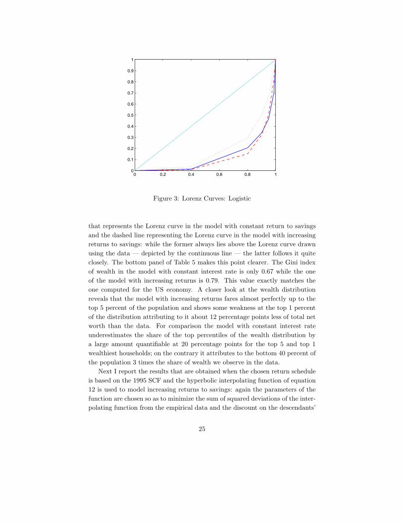
capital-output ratio of 3.04 which equates the target of 3. When the model isrun with constant returns agents need to be more impatient for market clearingto hold at a capital-output ratio of 3 so that β is now 0.989; as γ is kept constantthe bequest-to-earnings ratio changes to 2.15, double the one observed in thedata. Recall that the ratio involves median bequests, so this increase translatesinto an equalizing effect on the wealth distribution. Summary statistics for thesteady-state distributions are reported in Figure 3 and Table 5.

In the top panel of Table 5 I report the distribution of earnings in thedata and in the model. This distribution is exogenous to the model, howeverit is useful to assess its ability to match the empirical one. Recall from thecalibration section that the parameters governing the earnings process werechosen so as to match the overall and first-year earners Gini index. The firstof this calibration goal shows up in that the Gini index of the model and datareported in the table is the same. More importantly the calibrated earningsprocess can reproduce its empirical counterpart virtually perfectly up to thetop 5 percent of the distribution and only attributes a slightly lower share ofearnings to the top 1 percent. The latter is 14.8 percent in the data and 8.3in the model. The ability of the earnings process used here to match earningsinequality in the data is then very satisfactory; even at the top of the distributionthe difference is only a few percentage points, moreover this difference can bethough of as partially offsetting the omission of progressive taxation from themodel.

As far as the wealth distribution is concerned, Figure 3 gives a visual rep-resentation of the effects of increasing returns to savings. It is apparent thatthe small difference in returns faced by agents with different levels of assets issufficient to generate a substantial amount of extra wealth inequality comparedto the one implied by the assumption that all agents in the economy face thesame returns on asset holdings. This can be seen by comparing the dotted line

24

0 0.2 0.4 0.6 0.8 10

0.1

0.2

0.3

0.4

0.5

0.6

0.7

0.8

0.9

1

Figure 3: Lorenz Curves: Logistic

that represents the Lorenz curve in the model with constant return to savingsand the dashed line representing the Lorenz curve in the model with increasingreturns to savings: while the former always lies above the Lorenz curve drawnusing the data — depicted by the continuous line — the latter follows it quiteclosely. The bottom panel of Table 5 makes this point clearer. The Gini indexof wealth in the model with constant interest rate is only 0.67 while the oneof the model with increasing returns is 0.79. This value exactly matches theone computed for the US economy. A closer look at the wealth distributionreveals that the model with increasing returns fares almost perfectly up to thetop 5 percent of the population and shows some weakness at the top 1 percentof the distribution attributing to it about 12 percentage points less of total networth than the data. For comparison the model with constant interest rateunderestimates the share of the top percentiles of the wealth distribution bya large amount quantifiable at 20 percentage points for the top 5 and top 1wealthiest households; on the contrary it attributes to the bottom 40 percent ofthe population 3 times the share of wealth we observe in the data.

Next I report the results that are obtained when the chosen return scheduleis based on the 1995 SCF and the hyperbolic interpolating function of equation12 is used to model increasing returns to savings: again the parameters of thefunction are chosen so as to minimize the sum of squared deviations of the inter-polating function from the empirical data and the discount on the descendants’

25

0 0.2 0.4 0.6 0.8 10

0.1

0.2

0.3

0.4

0.5

0.6

0.7

0.8

0.9

1

Figure 4: Lorenz Curves: Hyperbolic

utility is set so as to match the ratio of median bequests to average earnings.The value of γ that achieves that is 0.25. As a consequence of the heavier dis-counting of descendants’ utility the value of β needed for market clearing climbsup to 1.013. The median bequest-to earnings ratio is 1.017 and capital-outputratio from the supply side is 3.016 confirming the excellent quality of the solu-tion to the market clearing and calibration system of equations. Results fromthis case are reported in Figure 4 and Table 6. 14 Once again the lorenz curveof the constant interest rate case lies above the one of the increasing returns andfurther from the data curve but differences are now smaller. This can be betterunderstood by looking at the corresponding table. As it can be seen by compar-ing the second and third row of the table the Gini index goes up from 0.68 to0.76 and the share of all the top percentiles of the wealth distribution increasessubstantially except for the top 1 percent of the population where extra wealthaccumulation brought about by the higher return is negligible. Correctly themodel with increasing return to savings cut by more than half the share of ag-gregate wealth held by the bottom 40 percent of the population. If we compare

14The nature of the experiment is the same as the one in the previous section: first the modelwith increasing returns to savings is solved, then this potential source of wealth inequality isshut off and the model is solved again. In particular as before, the intergenerational discountfactor is kept constant across the two experiments; notice that since γ has changed acrossthe experiments with different return functions the wealth distribution in the case of constantreturns will show some minor changes here as well

26

Table 6: Wealth Distribution: Hyperbolic Return FunctionPercentage share of Wealth by quantiles

Gini Bottom 40 Top 20 Top 10 Top 5 Top 1Data 0.78 1.35 79.5 66.1 53.5 29.5Model (H) 0.76 1.3 81.0 60.6 41.3 13.6Model (C) 0.68 3.2 71.7 51.5 34.4 11.1

the model with hyperbolic returns to the data we see that the model can matchperfectly the Gini index of wealth and the share of up to the top 10 percent ofthe population; it still does well at the top 5 percent of the distribution but theshare of the top 1 percent is under-predicted by a large amount.

6.2 Summary and Discussion

In this section I summarize the results of the previous section first, then Idiscuss the relation between the current model with the closest approach in theliterature, that is, the one based on entrepreneurship presented by Quadrini(2000). Table 7 reports the figures that are needed to develop the first point. Inthe first line of the table I report once more the wealth inequality statistics fromthe data. The second line performs a counterfactual experiment with those data,that is, it reports what the same distribution would be if the top 0.5 percentheld the same average net worth as the next half percentile, the one betweenthe 99.0 and the 99.5 percent wealthiest households. The third line reports theaverage of the two models’ steady state distribution obtained in the previoussection. This distribution is not the result of any particular run of the model:as it was said before the two different increasing return functions deliver anupper and lower bound of the wealth inequality that results when we introducein a model the fact that investment opportunities are related to wealth. Thebest assessment of this force will lie somewhere in between those bounds soreporting the average of the two distributions is a way to provide the readera quick access to it. Finally the last line reports the steady state distributionof a model with constant interest rate when γ is calibrated so that the modelgenerated bequest-to-earnings ratio is 1 as in the data, so it can be consideredthe “best” simulation for the constant return case.

If we first compare the two model distributions to the true data distributionwe see that increasing returns to savings do help getting a better match betweenthe two: the Gini index in this case is exactly equal to its data counterpart whileit is 9 points less in the constant interest case. Moreover the distribution in theincreasing returns world adheres quite well to the one in the data and onlydeparts from it substantially at the top 1 percent where it attributes only 50

27

Table 7: Wealth Distribution: SummaryPercentage share of Wealth by quantiles

Gini Bottom 40 Top 20 Top 10 Top 5 Top 1Data 0.78 1.35 79.5 66.1 53.5 29.5Data (99.5%) 0.77 1.6 75.8 60.0 45.1 16.8Model (L/H) 0.78 1.2 83.0 64.3 45.5 15.5Model (C) 0.69 2.6 72.6 51.8 33.4 11.2

percent of the true share. On the contrary the model with constant returnsshows great difficulties at matching the data starting from the top 5 percent ofthe distribution: it gives a share that is 20 percentage points below the true oneto the top 5 percent and about a third of the true value to the top 1 percent.

When we compare the models to the data that do not include the extra networth accumulated by the top 0.5 percent we see that the fit of both improves.However while the model with constant returns still attributes the top 5 and1 percent of the distribution only about two thirds of the shares of wealth inthe modified data, the model with increasing returns matches the distributionthat excludes the top 0.5 percent extra wealth virtually perfectly. This leadsus to the following two conclusions. First the fact that investment opportu-nities improve with wealth levels does add something to our understanding ofthe wealth distribution since it allows us to explain the accumulation behaviorof households up to the top 0.5 percent wealthiest families, while this is notwhat happens in a similar model with constant returns. Second, the fact thatthe top 0.5 of the distribution is left unaccounted suggests that the simple for-mulation of the properties of returns used here does not change the view, wellexpressed for example in Carroll (2000) that there is something special aboutwealth accumulation by the very rich.

Quadrini’s explanation based on entrepreneurship is a natural candidate inthis respect since even within the top 1 percent of the population the share ofentrepreneurs increases as we move further rightward in the tail of the distribu-tion: in the top 1 percent of the wealth distribution 65 percent of households areentrepreneurs, this fraction climbs up to 75 percent in the top 0.5 percent andto 82 percent in the top 0.25 percent.15 For this reason it is worth comparingthe present formulation of increasing returns to savings to the approach basedon entrepreneurship. In practice Quadrini models entrepreneurship as a set ofprojects of increasing size that an agent may have the chance to undertake. Inso doing the agent would add business profits to regular wage earnings. For

15These figures are based on the 1998 issue of the SCF and define an entrepreneurial house-hold one that has non-zero investment in closely held businesses.

28

each project size there is a range of wealth where the agent may undertake theproject but has to finance it partially with loans at a rate that is above marketrates. This specification is equivalent to a return function that in some rangesof wealth exhibits returns that are above the market interest. This is in partbecause any dollar invested raises the probability that the agent will be ableto take advantage of the extra profits from running a business —or one that islarger than the one he is already running—, in part because as long as he needsto finance the business through loaned funds, the marginal return to savingswill sum the intermediation cost to the market return. Otherwise the modelis a standard infinite-horizon buffer stock model. This latter fact implies thatparticular combinations of patience and returns to investment in the firm wouldmake the agent invest any amount of wealth. Indeed in his calibration the con-dition for boundedness of asset holdings is not met for entrepreneurs that areborrowing. However as the maximum firm size — the largest of the three pos-sible projects — is reached returns fall again to market levels and accumulationrapidly stops. By carefully choosing the size of entrepreneurial projects andtherefore the implicit return function Quadrini can reproduce the wealth distri-bution. My approach is simpler: I just estimate a return function from data andassess its quantitative impact on the wealth distribution. On the one hand thisapproach is more general since the fact that wealthier agents face higher returnsthrough different investment choices is not confined to entrepreneurs. On theother hand it misses some peculiar features of entrepreneurial activity like therole played by financial imperfections to increase the cost of external financingor the existence of idiosyncratic investment risk. 16 The other main differencebetween the current framework and the one in Quadrini is the assumption madehere that households have finite lives and form dynasties through ability andfinancial links. In a finite horizon model the mechanism that lies at the hearthof Quadrini’s paper, that is, the combination of patience and entrepreneurialreturns would not hold any more. It would then be interesting to see if andunder what conditions bequests, life-cycle savings and other issues that arisein this context would allow the results of the entrepreneurial model to survive.This is beyond the scope of the present paper and is left for future research.

7 Conclusions

The economic fortunes of the households in real economies are very unequal withwealth being substantially more concentrated than other measures like income

16Quadrini also assumes that entrepreneurial activity carries extra income risk magnifyingprecautionary savings of business households compared to workers. This aspect is not centralto the comparison with the model presented in this paper so I won’t elaborate it further

29

and earnings. This fact has attracted a lot of attention among macroeconomists.The basic framework of precautionary saving outlined in Aiyagari (1994) hasproven capable of reproducing the fact reported above qualitatively, but notquantitatively leading to successive extensions that include different features,like social security, intergenerational links, entrepreneurship or heterogeneouspreferences but retain the basic assumption that a single asset is available inthe economy. This paper explicitly acknowledges the fact that in reality thereis a menu of assets with different returns that households may use to carry outtheir saving plans and that there is a systematic positive relationship betweenasset holdings and the return to these holdings.

To accomplish this task I have considered a model that blends the life-cycleand dynastic framework where I assume that agents face a return to their savingsthat is increasing in the level of assets they hold. This feature is able to increasesubstantially the level of wealth inequality compared to the standard case ofconstant returns. As a matter of fact the model is able to account for the U.S.distribution of wealth up to the 99.5 percentile, whereas a similarly calibratedmodel that omits the relationship between asset holdings and returns cannot.The model still fails to match the huge fortunes that are accumulated by a fewwealthy households at the very top — 0.5 percent — of the distribution. Thissupports the view that some other mechanism must be at work for this group.Entrepreneurship as proposed by Quadrini or the capitalist spirit as proposedby Carroll are two possibilities. Integrating those two theories in a full life-cyclemodel with bequest like the one proposed here is left for future research.

Appendix

A Data Construction

In this appendix I describe briefly the construction of the household portfoliosfrom SCF data. Family asset holdings were classified into eight categories: liquidaccounts, bonds, stocks, other financial assets, primary residence, investmentreal estate, business equity and other non financial assets. Liabilities were clas-sified into four broad groups: mortgage and other loans on primary residence,other property loans, credit card balances and a residual category that includesother type of debt. The purpose of this classification is to reduce the complexityof household portfolios to a small number of asset types to which we can assignreturn data. The classification proposed sometimes does not overlap perfectlywith the one in the SCF thus requiring some imputations. This is the case of

30

defined contribution pension plans, IRA and Keogh accounts and trusts.17 Inthese cases the SCF reports qualitative information about how these accountswere invested. An example of the list of answers proposed to the respondent tothe SCF questionnaire is: mostly stock, mostly bonds, a combination of the twoor a menu of other types of assets. In this case if the answer was mostly stocksor mostly bonds I considered the whole account invested in stock or bond, ifthe answer was a combination, the imputation was half to stocks and half tobonds, in the other cases the account was included in the residual category ofthe classification. Summarizing the exact description of the single items in theclassification used here is:

- Liquid accounts: checking and savings accounts, money market mutualfunds, cash call accounts at brokers, certificates of deposits plus all ofthe previous items held through retirement accounts, trusts and othermanaged accounts.

- Bonds: all local, state, federal, corporate and foreign bonds held directly,through mutual funds or through retirement accounts, trusts and othermanaged accounts.

- Stock: all stock owned directly or through mutual funds, retirement ac-counts, trusts and other managed accounts.

- Other financial assets: this category includes a broad set of assets rang-ing from cash value of life insurance policies, to loans to friends. It alsoincludes the share of retirement accounts, trusts and other managed ac-counts invested in assets other than liquid, bonds and stocks of for whichno investment answer was reported. Finally it includes mutual funds notclassified.

- Primary residence: value of home, mobile home plus land and site whereit stands.

- Investment real estate: value of all other property.

- Business: value of equity in closely held firms of any legal form.

- Other nonfinancial assets: vehicles, jewelry, artwork, airplanes and a largenumber of other possible real assets.

Once the information on assets and liabilities holdings was classified, total networth was computed and the households were ordered based on it. For each

17Except for the imputations, the classification follows the one in Bertaut and Starr-McCluer(2000) to which the reader is referred for more details than those reported in this appendix.

31

of the net worth percentile group defined in the main text the share of eachcategory of asset and total assets were computed. These data formed the basison which the empirical return function was constructed.

B Numerical Solution Method

The methods used to solve the model are quite standard and the interestedreader is referred to Rıos-Rull (1998) for a detailed account. What I will do inthis section is first to give a short outline of the procedure used and then todescribe in more detail the method used to solve the dynastic dynamic program-ming problem. As far as the first part is concerned the steps are the following:

1. Guess initial values of the intergenerational discount factor γ and the taxrate on bequests τe.

2. Guess values for the subjective discount factor β and the income tax rateτ .

3. Solve the dynasty optimization problem and obtain the decision rules forassets and consumption. The procedure followed implied computing thevalue function at each age and finding the decision rules by maximizingthe right-hand side of the Bellman equation rather than finding the zeroof the associate euler equation. More details are given below.

4. Use the decision rules from step 3 and random sequences from the survivaland labor endowment processes to simulate the economy, obtain aggregateasset holdings and tax revenues; if the market clearing and governmentbudget balance conditions are met move on, else go back to 2.

5. If the bequest-to-earnings and the share of estate tax revenue in GDPtargets are met then move on, else go back to 1.

6. Compute the statistics of interest on the steady state distribution.

For the simulation of the economy the history of 40000 dynasties for 3000 periodswere used; further increasing those numbers did not affect the results. Giventhat a simple condition to insure that asset holdings are bounded above couldnot be found particular care was taken to avoid that the results could be anartefact of the finite simulation horizon. In practice I kept track of the maximumrealized value of asset holdings in each period and checked the following: firstthat it was always well below the upper bound of the domain over which thevalue function was approximated and second that it did not trend upward inthe simulation.

32

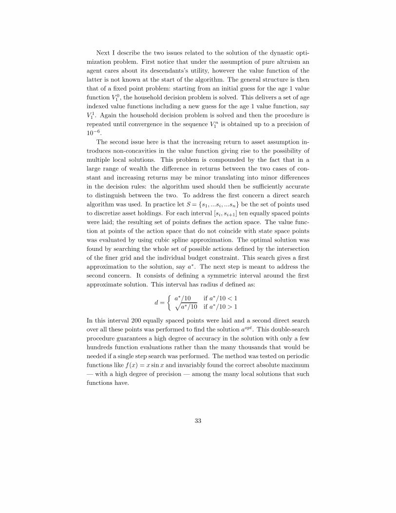
Next I describe the two issues related to the solution of the dynastic opti-mization problem. First notice that under the assumption of pure altruism anagent cares about its descendants’s utility, however the value function of thelatter is not known at the start of the algorithm. The general structure is thenthat of a fixed point problem: starting from an initial guess for the age 1 valuefunction V 0

1 , the household decision problem is solved. This delivers a set of ageindexed value functions including a new guess for the age 1 value function, sayV 1

1 . Again the household decision problem is solved and then the procedure isrepeated until convergence in the sequence V n

1 is obtained up to a precision of10−6.

The second issue here is that the increasing return to asset assumption in-troduces non-concavities in the value function giving rise to the possibility ofmultiple local solutions. This problem is compounded by the fact that in alarge range of wealth the difference in returns between the two cases of con-stant and increasing returns may be minor translating into minor differencesin the decision rules: the algorithm used should then be sufficiently accurateto distinguish between the two. To address the first concern a direct searchalgorithm was used. In practice let S = {s1, ...si, ...sn} be the set of points usedto discretize asset holdings. For each interval [si, si+1] ten equally spaced pointswere laid; the resulting set of points defines the action space. The value func-tion at points of the action space that do not coincide with state space pointswas evaluated by using cubic spline approximation. The optimal solution wasfound by searching the whole set of possible actions defined by the intersectionof the finer grid and the individual budget constraint. This search gives a firstapproximation to the solution, say a∗. The next step is meant to address thesecond concern. It consists of defining a symmetric interval around the firstapproximate solution. This interval has radius d defined as:

d ={

a∗/10 if a∗/10 < 1√a∗/10 if a∗/10 > 1

In this interval 200 equally spaced points were laid and a second direct searchover all these points was performed to find the solution aopt. This double-searchprocedure guarantees a high degree of accuracy in the solution with only a fewhundreds function evaluations rather than the many thousands that would beneeded if a single step search was performed. The method was tested on periodicfunctions like f(x) = x sin x and invariably found the correct absolute maximum— with a high degree of precision — among the many local solutions that suchfunctions have.

33

References

[1] Aiyagari, S.R. (1994). “Uninsured Idiosyncratic Risk and Aggregate Sav-ing”. Quarterly Journal of Economics, 109(3): 659-684.

[2] Barsky R. B., Juster F. T., Kimball M. S. and Shapiro M.D. (1997). “Pref-erence Parameters and Behavioral Heterogeneity: An Experimental Ap-proach in the Health and Retirement Study”. Quarterly Journal of Eco-nomics, 112 (2): 537-579.

[3] Bertaut C. and Starr-McCluer M. (2000). “Household Portfolios in theUnited States”. Federal Reserve Board of Governors, Finance and Eco-nomics Discussion Paper : 26 (April).

[4] Brent R. (1973). “Algorithms for Minimization without Derivatives”. En-glewood Cliffs, NJ: Prentice-Hall.

[5] Budrıa-Rodrıguez S., Dıaz-Gimenez J., Quadrini V. and Rıos-Rull J.-V.(2002). “Updated Facts on the U.S. Distributions of Earnings, Income andWealth”. Federal Reserve Bank of Minneapolis Quarterly Review, 26, (Sum-mer): 2-35.

[6] Cagetti M. and De Nardi M. (2002). “Entrepreneurship, Frictions andWealth”. Federal Reserve Bank of Minneapolis Working Paper 620.

[7] Carroll C.D. (2000). “Why Do the Rich Save So Much ?”. In: J. B. Slem-rod, (Ed). “Does Atlas Shrug? The Economic Consequences of Taxing theRich”. Cambridge, MA: Harvard University Press,

[8] Castaneda A., Dıaz-Gimenez J. and Rıos-Rull J.-V. (2003). “Accounting forthe U.S. Earnings and Wealth Inequality”. Journal of Political Economy.111(4):818-857.

[9] Cocco J., Gomes F. and Maenhout P. (2005). “Consumption and PortfolioChoice over the Life Cycle”. Review of Financial Studies. 18(2): 491-533.

[10] Conesa M. and Krueger D. (1999). “Social Security Reform with Hetero-geneous Agents”. Review of Economic Dynamics, 2: 757-795.

[11] De Nardi M. (2004). “Wealth Inequality and Intergenerational Links”. ”.Review of Economic Studies, 71: 743-768.

[12] Dıaz-Gimenez J., Quadrini V. and Rıos-Rull J.-V. (1997), “Dimensionsof Inequality: Facts on the U.S. Distribution of Earnings, Income andWealth”. Federal Reserve Bank of Minneapolis Quarterly Review, 21,(Spring): 3-21.

34

[13] Domeij D. and Klein P. (2002). “Public Pensions: To What Extent Do TheyAccount for Swedish Wealth Inequality ?”. Review of Economic Dynamics,5: 503-534.

[14] Gentry W. M. and Hubbard G.R. (2001). “Entrepreneurship and HouseholdSaving”. National Bureau of Economic Research, Working Paper No. 7894.

[15] Goetzmann W. N. and Spiegel M. (2000). “The Policy Implications of Port-folio Choice in Underserved Mortgage Markets”. Yale International Centerfor Finance. Working Paper 00-18.

[16] Guiso L., Haliassos M. and Jappelli T. eds. (2002). “Household Portfolios”.Cambridge and London: MIT press.

[17] Guiso L., Sapienza P. and Zingales L. (2004). “The Role of Social Capitalin Financial Development”. American Economic Review. 94: 526-556.

[18] Hansen G. (1993). “The Cyclical and Secular Behaviour of the LabourInput: Comparing Efficiency Units and Hours Worked”. Journal of AppliedEconometrics. 8(1): 71-80.

[19] Heaton J. and Lucas D. (2000) “Portfolio Choice and Asset Prices: TheImportance of Entrepreneurial Risk”. Journal of Finance. 55(3), pp. 1163-1198.

[20] Hong H., Kubik J. and Stein J. (2001). “Social Interaction and Stock Mar-ket Participation”. National Bureau of Economic Research, Working PaperNo. 8358.

[21] Hubbard G. R., Skinner J. and Zeldes S. (1995). “Precautionary Savingand Social Insurance”. Journal of Political Economy. 103(2): 360-399.

[22] Huggett M. (1996). “Wealth Distribution in Life-Cycle Economies”. Jour-nal of Monetary Economics, 38(3):469-494.

[23] Huggett M. and Ventura G. (2000). “Understanding Why High IncomeHouseholds Save More than Low Income Households”. Journal of MonetaryEconomics, 45: 361-397.

[24] Hurd M. and Smith J. (2002). “Expected Bequests and Their Distribution”.National Bureau of Economic Research, Working Paper No. 9142.

[25] Hurst E., Luoh M.C. and Stafford F.P. (1998), “The Wealth Dynamics ofAmerican Families, 1984-94”. Brookings Papers on Economic Activity, 1:267-329.

35

[26] Jagannathan R., McGrattan E. and Scherbina A. (2000). “The DecliningU.S. Equity Premium”. Federal Reserve Bank of Minneapolis QuarterlyReview, 24 (Fall): 3-19.

[27] Kennickell A. B., Starr-McCluer M. and Surette B.J. (2000). “RecentChanges in U.S. Family Finances: Results from the 1998 Survey of Con-sumer Finances”. Federal Reserve Bulletin, (January): 1-29.

[28] Krusell P. and Smith A.A. (1998). “Income and Wealth Heterogeneity inthe Macroeconomy”. Journal of Political Economy, 106(5): 867-896.

[29] Moskowitz T. and Vissing-Jørgensen A. (2002). “The Returns to En-trepreneurial Investment: A Private Equity Premium Puzzle ?”. AmericanEconomic Review, 92(4): 745-778.

[30] Paiella P. (2001). “Limited Financial Market Participation: A Transaction-Cost Based Explanation”. The Institute for Fiscal Studies. WP 01/06.

[31] Quadrini V. (2000). “Entrepreneurship, Saving and Social Mobility”. Re-view of Economic Dynamics, 3,(1): 1-40.

[32] Rıos Rull J.V. (1999). “Computation of Equilibria in Heterogeneous-AgentEconomies ”. In: Marimon R. and Scott A. Eds. “Computational Methodsfor the Study of Dynamic Economies”. Oxford and New York: OxfordUniversity Press.

[33] Samwick A.A. (2000). “Portfolio Responses to Taxation: Evidence fromthe End of the Rainbow”.In: J. B. Slemrod, (Ed). “Does Atlas Shrug? TheEconomic Consequences of Taxing the Rich”. Cambridge, MA: HarvardUniversity Press.

[34] Vissing-Jørgensen A. (2001). “Towards an Explanation of Household Port-folio Choice Heterogeneity: Nonfinancial Income and Participation CostStructures”. Working Paper. University of Chicago.

[35] Edward N. Wolff. (2000). “Who Are the Rich ? A Demographic Profileof High-Income and High-Wealth Americans”. In: J. B. Slemrod, (Ed).“Does Atlas Shrug? The Economic Consequences of Taxing the Rich”.Cambridge, MA: Harvard University Press.

36

Our papers can be downloaded at:

http://cerp.unito.it

CeRP Working Paper Series

N° 1/00 Guido Menzio Opting Out of Social Security over the Life Cycle

N° 2/00 Pier Marco Ferraresi Elsa Fornero

Social Security Transition in Italy: Costs, Distorsions and (some) Possible Correction

N° 3/00 Emanuele Baldacci Luca Inglese

Le caratteristiche socio economiche dei pensionati in Italia. Analisi della distribuzione dei redditi da pensione (only available in the Italian version)

N° 4/01 Peter Diamond Towards an Optimal Social Security Design

N° 5/01 Vincenzo Andrietti Occupational Pensions and Interfirm Job Mobility in the European Union. Evidence from the ECHP Survey

N° 6/01 Flavia Coda Moscarola The Effects of Immigration Inflows on the Sustainability of the Italian Welfare State

N° 7/01 Margherita Borella The Error Structure of Earnings: an Analysis on Italian Longitudinal Data

N° 8/01 Margherita Borella Social Security Systems and the Distribution of Income: an Application to the Italian Case

N° 9/01 Hans Blommestein Ageing, Pension Reform, and Financial Market Implications in the OECD Area

N° 10/01 Vincenzo Andrietti and Vincent Hildebrand

Pension Portability and Labour Mobility in the United States. New Evidence from the SIPP Data

N° 11/01 Mara Faccio and Ameziane Lasfer

Institutional Shareholders and Corporate Governance: The Case of UK Pension Funds

N° 12/01 Roberta Romano Less is More: Making Shareholder Activism a Valuable Mechanism of Corporate Governance

N° 13/01 Michela Scatigna Institutional Investors, Corporate Governance and Pension Funds

N° 14/01 Thomas H. Noe Investor Activism and Financial Market Structure

N° 15/01 Estelle James How Can China Solve ist Old Age Security Problem? The Interaction Between Pension, SOE and Financial Market Reform

N° 16/01 Estelle James and Xue Song

Annuities Markets Around the World: Money’s Worth and Risk Intermediation

N° 17/02 Richard Disney and Sarah Smith

The Labour Supply Effect of the Abolition of the Earnings Rule for Older Workers in the United Kingdom

N° 18/02 Francesco Daveri Labor Taxes and Unemployment: a Survey of the Aggregate Evidence

N° 19/02 Paolo Battocchio Francesco Menoncin

Optimal Portfolio Strategies with Stochastic Wage Income and Inflation: The Case of a Defined Contribution Pension Plan

N° 20/02 Mauro Mastrogiacomo Dual Retirement in Italy and Expectations

N° 21/02 Olivia S. Mitchell David McCarthy

Annuities for an Ageing World

N° 22/02 Chris Soares Mark Warshawsky

Annuity Risk: Volatility and Inflation Exposure in Payments from Immediate Life Annuities

N° 23/02 Ermanno Pitacco Longevity Risk in Living Benefits

N° 24/02 Laura Ballotta Steven Haberman

Valuation of Guaranteed Annuity Conversion Options

N° 25/02 Edmund Cannon Ian Tonks

The Behaviour of UK Annuity Prices from 1972 to the Present

N° 26/02 E. Philip Davis Issues in the Regulation of Annuities Markets

N° 27/02 Reinhold Schnabel Annuities in Germany before and after the Pension Reform of 2001

N° 28/02 Luca Spataro New Tools in Micromodeling Retirement Decisions: Overview and Applications to the Italian Case

N° 29/02 Marco Taboga The Realized Equity Premium has been Higher than Expected: Further Evidence

N° 30/03 Bas Arts Elena Vigna

A Switch Criterion for Defined Contribution Pension Schemes

N° 31/03 Giacomo Ponzetto Risk Aversion and the Utility of Annuities

N° 32/04 Angelo Marano Paolo Sestito

Older Workers and Pensioners: the Challenge of Ageing on the Italian Public Pension System and Labour Market

N° 33/04 Elsa Fornero Carolina Fugazza Giacomo Ponzetto

A Comparative Analysis of the Costs of Italian Individual Pension Plans

N° 34/04 Chourouk Houssi Le Vieillissement Démographique : Problématique des Régimes de Pension en Tunisie

N° 35/04 Monika Bütler Olivia Huguenin Federica Teppa

What Triggers Early Retirement. Results from Swiss Pension Funds

N° 36/04 Laurence J. Kotlikoff Pensions Systems and the Intergenerational Distribution of Resources

N° 37/04 Jay Ginn Actuarial Fairness or Social Justice? A Gender Perspective on Redistribution in Pension Systems

N° 38/05 Carolina Fugazza Federica Teppa

An Empirical Assessment of the Italian Severance Payment (TFR)

N° 39/05 Anna Rita Bacinello Modelling the Surrender Conditions in Equity-Linked Life Insurance

N° 40/05 Carolina Fugazza Massimo Guidolin Giovanna Nicodano

Investing for the Long-Run in European Real Estate. Does Predictability Matter?

N° 41/05 Massimo Guidolin Giovanna Nicodano

Small Caps in International Equity Portfolios: The Effects of Variance Risk.

N° 42/05 Margherita Borella Flavia Coda Moscarola

Distributive Properties of Pensions Systems: a Simulation of the Italian Transition from Defined Benefit to Defined Contribution

N° 43/05 John Beshears James J. Choi David Laibson Brigitte C. Madrian

The Importance of Default Options for Retirement Saving Outcomes: Evidence from the United States

N° 44/05 Henrik Cronqvist Advertising and Portfolio Choice

N° 45/05 Claudio Campanale Increasing Returns to Savings and Wealth Inequality