INCORPORATION OF LIQUIDITY RISKS INTO EQUITY PORTFOLIO RISK ESTIMATES

Dan diBartolomeo September 2010

GOALS FOR THIS TALKAssert that liquidity of a stock is properly measured as the expected price change, given a proposed trade of particular size in a particular time frame

Propose a conceptual framework of equity security risk that considers price movements as the accumulation of market impact over a set of transactions

Describe our estimation of market impact from tick data, under boundary conditions

Derive a joint measure of equity risk and liquidity risk that accounts for the greater liquidity risk of larger portfolios

A MICROSTRUCTURE VIEW OF EQUITY RISK

The process of price discovery for stocks arises from balancing the supply available from willing sellers to the demand from willing buyersSecurity returns are just the accumulation of the price impacts of the individual trades within that time periodThe volatility of returns manifests changes in the imbalance between buyers and sellers over time, but not all observed returns are informativeIf we can forecast the potential for imbalances to arise, we can forecast equity risk more efficientlyThe larger our own portfolio is, the greater the potential for we ourselves to create imbalances and contribute to risk

WHAT MAKES PEOPLE BUY OR SELL A PARTICULAR STOCK?

They WANT to trade the stockThey believe the information that supports a valid forecast of abnormal future return

They HAVE to trade the stockThey are trading to implement a change in asset allocationThey are trading to implement a cash versus futures arbitrage trade on a stock indexThey are a mutual fund or ETF sponsor responding to investor cash flows in or out of the portfolioThey are hedge fund that is forced to transact because of a margin callThey are forced to cover a short position by having the stock called

THE POTENTIAL FOR “HAVE TO’S”

We can fundamentally evaluate the potential for “have to” trades

Index arbitrage trades only occur with index constituents and we know the open interest in futuresShort interest information is publishedWe know which big hedge and mutual funds have big positions in particular stocksWe have somewhat out of date information on full mutual fund holdings and cash flow statisticsWe have up to date information on ETF flows

THE POTENTIAL FOR “WANT TO” TRADES

Investors are responding to information, so just measure variations in the volume of information about a particular stock over timeCapture the flow of news text coming over services such as Dow-Jones, Reuters and Bloomberg

Ravenpack and Thomson Reuters offer real time statistical summariesof the amount and content of text news distributedLexicons of popular phrases are used to score the content of text as “good news” or “bad news”See diBartolomeo, Mitra and Mitra (2009)

Judge retail investor interest directly by measuring the number of Google and Yahoo searches on ticker symbols

Da, Engleberg and Gao (2009)Avoid company names to eliminate product or service related searchesTry it yourself with Google Trends

IMPROVING SHORT HORIZON RISK ESTIMATESPrice impact generated by “have to” trades in individual stocks is transient, but can become permanent if sufficiently widespread to impact the real economyPrice impact generated by “want to” trades arise from informed traders and is likely to be long lastingWe should be able to observe larger and more dispersed imbalances between buyers and sellers for stocks that are larger in potential for “have to” and “want to” tradesWe now have a new way to calibrate equity risk estimates

Observed variations in returns (i.e. the usual way)Observed time series variation of imbalances between buyers and sellers

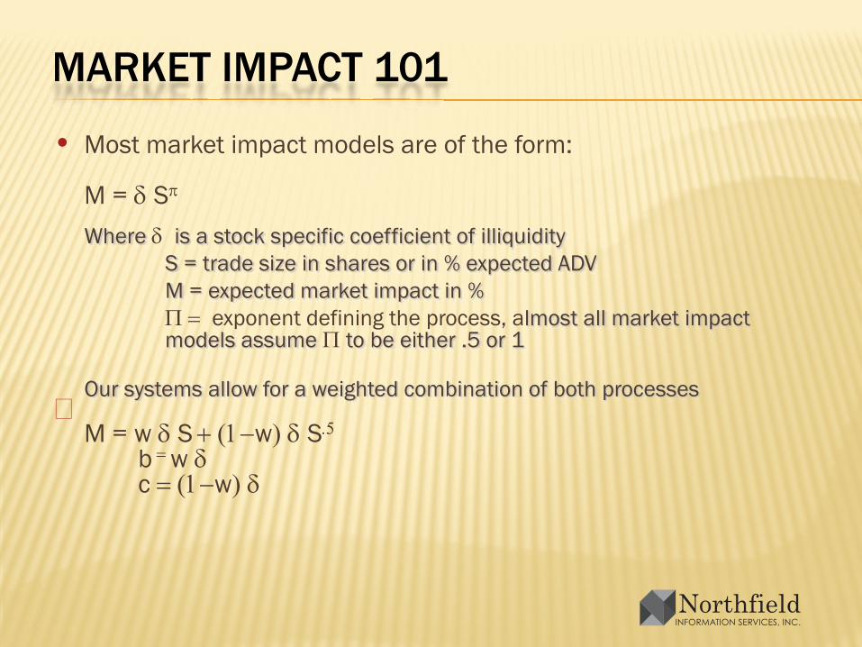
MARKET IMPACT 101

• Most market impact models are of the form:

M = δ Sπ

Where δ is a stock specific coefficient of illiquidityS = trade size in shares or in % expected ADVM = expected market impact in %Π = exponent defining the process, almost all market impact models assume Π to be either .5 or 1

Our systems allow for a weighted combination of both processes

M = w δ S + (1−w) δ S.5

b = w δc = (1−w) δ

MEASURING BUYER/SELLER IMBALANCE

We adopt the model of Lee and Ready (1991) for our definition of “buyer” and “seller” trading volume

Assumes that if a trade occurred on an uptick in price this was a “buyer” trade that was accommodated by a liquidity providerIf a trade occurs on a downtick in price, assume that this was a “seller” trade that was accommodated by a liquidity providerIf a trade occurs on a flat tick (no price change) it is assumed to be of the same character as the previous trade

Define “imbalance”

S = (buying volume – selling volume) / total volume

Accumulate daily volume imbalances

THE PROBLEM WITH TICK DATA

Our data consists of every tick for the past fourteen years of trading on a globally representative sample of five thousand stocks classified into about one hundred thirty groups by country and market capitalization. The data is obtained from Reuters

It must be noted that the Reuters data is organized by RIC code, so if a stock is traded at more than one venue (e.g. multiple exchanges, ECNs), the trading at each venue will be treated separately and may require consolidation. The data set also includes every quote

The combined size of the entire Reuters tick data set for all securities worldwide approaches three hundred terabytes. The computational effort associated with using the tick data method is considerable!

TIMES SERIES COST ESTIMATION

Estimate via three rank time series regressions where daily return is the dependent variable using a three month time windowR% = b S + c S.5

We estimate b directly. We do two separate estimations for c for positive and negative imbalances

Use Bayes’s Theorem to combine the three regression coefficients

Obtain w, δ, Π

While the tick method is normally estimated based on percentage imbalance of daily volume, we can rescale the imbalance values by the relationship of average daily volume to shares outstanding to switch to cost per share units

REFINEMENT #1: BOUNDARY CONDITIONS

Constrain the range of the regression coefficients with boundary conditions

Market impact comes from information leakage. Other people figure out what you are doing and change their trading from their knowledge of your intentThe worst case scenario for information leakage is a hostile takeover. You are going to buy up all the shares of a firm and publicly announce you are doing it.

The coefficients should be constrained to produce maximum buying costs similar to the expected premium in a hostile takeover for a trade of all shares outstanding (typically 25 to 70%)

The maximum cost of a “sell” cannot exceed 100% even for a trade of all shares outstanding

REFINEMENT #2: LARGE TRADES

The distribution of trade size within a day often has a large degree of skew, leading to unintuitive results

CRH PLC (Ireland) on 14 May 2009 Volume imbalance -30.25% but total return is +3.3 so the relationship has the wrong signApproximately two million shares trade in 722 tradesMedian trade size is 400 shares, average trade size is 2783 shares, maximum trade size is 300,000 sharesLarge sells are much more frequent than large buys in the data

Solution is to separate out very large institutional trades from the sample and estimate separately

Measure instantaneous impact as change from the previous trade price, accumulate over large trades onlyDefine “large” trades” being > 2% daily volume and having a Z-score > X (e.g. 2) in the log of shares traded per trade for that day

REFINEMENT #3: USE QUOTES

Confirm the classification of “buyer” and “seller” initiated trades by comparing execution prices to the previous bid-asked quote

Transactions occurring at or above the previous asking price are assumed to be initiated by a buyer and accommodated by a liquidity provider

Transactions occurring at or below the previous bid price are assumed to be initiated by a seller and accommodated by a liquidity provider

REFINEMENT #4: ADJUST FOR SHIFTS IN VOLATILITY

Our times series estimates of coefficients b and c are based on data for the three month trailing months

To the extent we know believe that a given stock is expected to more volatile now than it was on average during the sample period, we should adjust the value of b and c to reflect the relationship between volatility and expected market impact

bt = b * (St /AVERAGE[St-60 to t-1])K

ct = c * (St /AVERAGE[St-60 to t-1])K

Where S(t) = expected volatility of stock x at date t K = w + .5 (1-w)

We can use this relationship to estimate costs in crisis conditions from the concurrent volatility spikes

ALTERNATIVE ESTIMATION OF COSTS

We can also estimate a factor model of market impact

Eit = % price change / % imbalance for stock i on day tEit = b1t σit + b2t log Mci + other factors

Where Eit = price elasticity of stock i on day tσit = forecast volatility of stock i on day tMci = log of total market cap of country c of stock i

Separate information into four regressions: positive and negative imbalances each assuming π = 1 and = .5

Combine regressions using Bayes’s TheoremTake 20 day volume-weighted average across timeThis model will be available daily for a fee starting July

SAVING YOU A LITTLE MONEY

We can also use the existing Northfield cost model that has been provided free on a monthly basis with all equity risk models, since May 2009

This model estimates illiquidity for all stocks globally based on observable serial correlation in daily returns.

The higher the cost of trading a stock, the lower the number of sign changes in a daily return times series will be.

Implied serial correlation was calibrated against a database of more than 1.5 million anonymous actual trade costs

THE NUMBERS ADD UPIf we believe in linear factor risks and we also believe in price risk as the accumulation of market over many trades we would expect that the exponent on the market impact formula should be close to one for trading over fixed time intervals

This means that the “square root” aspect of market impact arises from traders stretching out large trades over long time horizons to reduce costs

Strong empirical evidence supports this hypothesisSee “Market Impact Monthly” research reports from JPMorgan

THE FAULT DEAR BRUTUS LIES NOT IN OUR STARS BUT IN OURSELVES

Conventional portfolio risk calculations deal only in security weights

Ignores the magnitude of portfolio valueIgnores the potential for our own “have to” tradesTheoretical discussion in Acerbi and Scandolo (2007)Assets have prices, but portfolios have values that are functions of a liquidity policy

Given the nature of our own portfolio, we can estimate the potential for our own “have to” trades Certain types of “have to” trades are likely to highly correlated across managers of similar style and portfolio composition because they are pro-cyclical

October 1987 with portfolio insurance and index arbitrageAugust 2007 with hedge fund margin calls

LIQUIDITY POLICIES AND RISK

We can formulate a liquidity policy as:

We have to be able to liquidate X% of the portfolio in N trading days

Given our models of cost, we can estimate the cost of liquidationTo adjust our portfolio risk estimate for liquidity

Convert our portfolio volatility estimate to parametric Value at Risk for the length of time specified in our liquidity policyAdd the expected cost of fulfilling liquidation to VaRConvert the new VaR value back to the equivalent volatility

QUICK EXAMPLE

Our liquidity policy: We must be able to liquidate 30% of the portfolio in 10 trading days

Our estimated portfolio volatility is 25% per yearAssume 3 standard deviation VaR (covers 99.8% of normal distribution)% Parametric VaR = 14.94 [25 * 3 * (10/252)^.5]Assume our forecast liquidation cost is 4%% Parametric VaR with Cost = 18.94 [14.94 + 4]Revised portfolio volatility = 31.70 [18.94 / 3 * (252/10)^.5]

Volatility estimate increased by more than 23%

ALTERNATIVE FORMULATION: LIQUIDITY DRAG

As positions in a portfolio get larger and larger, executing trades at reasonable cost will take longer and longer, reducing opportunity to earn active returnsAn extreme case is fully illiquid investments such as real estate or private equity

You put the first dollars in the “best” deal, the next dollars in the second best deal and so onThe more money you allocate to an asset, the lower the expected returns become

Experiment on a small childSend them to the candy store with a large amount of money. They will buy all sorts of stuff and end up with an upset stomachSend them to the candy store with a small amount of money. They will buy just their favorite candy and be happy

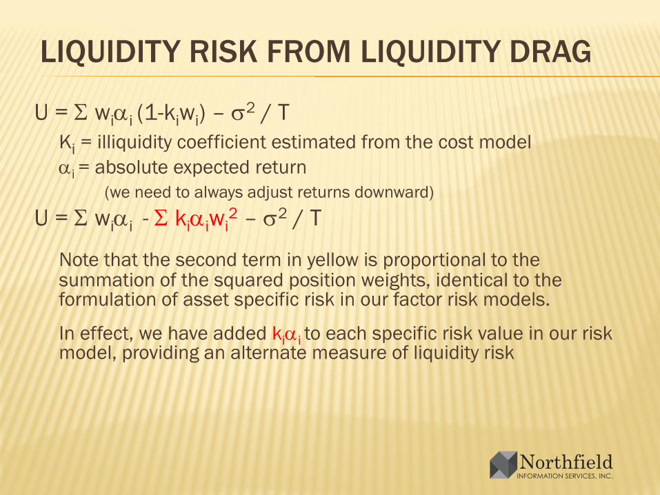
LIQUIDITY RISK FROM LIQUIDITY DRAG

U = Σ wiαi (1-kiwi) – σ2 / T Ki = illiquidity coefficient estimated from the cost modelαi = absolute expected return

(we need to always adjust returns downward)

U = Σ wiαi - Σ kiαiwi2 – σ2 / T

Note that the second term in yellow is proportional to the summation of the squared position weights, identical to the formulation of asset specific risk in our factor risk models.

In effect, we have added kiαi to each specific risk value in our risk model, providing an alternate measure of liquidity risk

CONCLUSIONS

Liquidity risk is a critical issue for most investors, particularly those that are either very large or are leveragedEstimation of trading costs associated with liquidity needs can be efficiently accomplished through our tick based model, as well as other models of costVariability in buyer/seller imbalance information can be used as a metric for short horizon riskWe have presented two methods for including liquidity risk into portfolio risk estimates