
Incorporating travel time reliability in the estimation of
100
Incorporating travel time reliability in the estimation of assignment models December 2011 A W Brennand NZ Transport Agency research report 464
Transcript of Incorporating travel time reliability in the estimation of

Incorporating travel time reliability in the
estimation of assignment models
December 2011
A W Brennand
NZ Transport Agency research report 464

ISBN 978-0-478-38079-8 (print)
ISBN 978-0-478-38078-1 (electronic)
ISSN 1173-3756 (print)
ISSN 1173-3764 (electronic)
NZ Transport Agency
Private Bag 6995, Wellington 6141, New Zealand
Telephone 64 4 894 5400; facsimile 64 4 894 6100
www.nzta.govt.nz
Brennand, AW (2011) Incorporating travel time reliability in the estimation of assignment models. NZ
Transport Agency research report 464. 100pp.
Tau Squared Ltd, PO Box 39378, Wellington Mail Centre, New Zealand.
This publication is copyright © NZ Transport Agency 2011. Material in it may be reproduced for personal
or in-house use without formal permission or charge, provided suitable acknowledgement is made to this
publication and the NZ Transport Agency as the source. Requests and enquiries about the reproduction of
material in this publication for any other purpose should be made to the Research Programme Manager,
Programmes, Funding and Assessment, National Office, NZ Transport Agency, Private Bag 6995,
Wellington 6141.
Keywords: assignment, coefficient of variation, congestion index, NZ Transport Agency, reliability, route
choice, travel time, variability
An important note for the reader
The NZ Transport Agency is a Crown entity established under the Land Transport Management Act 2003.
The objective of the Agency is to undertake its functions in a way that contributes to an affordable,
integrated, safe, responsive and sustainable land transport system. Each year, the NZ Transport Agency
funds innovative and relevant research that contributes to this objective.
The views expressed in research reports are the outcomes of the independent research, and should not be
regarded as being the opinion or responsibility of the NZ Transport Agency. The material contained in the
reports should not be construed in any way as policy adopted by the NZ Transport Agency or indeed any
agency of the NZ Government. The reports may, however, be used by NZ Government agencies as a
reference in the development of policy.
While research reports are believed to be correct at the time of their preparation, the NZ Transport Agency
and agents involved in their preparation and publication do not accept any liability for use of the research.
People using the research, whether directly or indirectly, should apply and rely on their own skill and
judgement. They should not rely on the contents of the research reports in isolation from other sources of
advice and information. If necessary, they should seek appropriate legal or other expert advice.

Acknowledgements
The author wishes to acknowledge and thank Fraser Fleming and Bob Hu of Opus International
Consultants Ltd for their contribution to section 5 of this report which included the modelling exercises
undertaken. The Wellington Regional Council is acknowledged for supplying travel time survey data.
John Bolland of John Bolland Consulting Ltd and Tim Kelly of Tim Kelly Transportation Planning Ltd, who
were project peer reviewers for this study, are thanked for their helpful and insightful contributions to this
study.
Abbreviations and acronyms
AADT annual average daily traffic
CIt congestion index
CVt coefficient of variation of travel time
%RMSE root mean square error expressed as a percentage
GEH a modified chi-squared statistic used in traffic model validation
HCV heavy commercial vehicle
NB northbound
NZTA New Zealand Transport Agency
R2
regression coefficient squared
RMGEH2
root mean square GEH – a non-standard validation statistic
SB southbound
SH state highway
V/C traffic volume to capacity ratio
WTM Wellington Traffic Model
WTSM Wellington Transport Strategic Model

5
Contents
Executive summary ................................................................................................................................................................. 7
Abstract ....................................................................................................................................................................................... 10
1 Introduction ................................................................................................................................................................ 11
2 Literature review ..................................................................................................................................................... 13
2.1 Preamble .................................................................................................................. 13
2.2 Where and why accounting for travel time reliability has been used ....................... 13
2.2.1 Economic consequences ............................................................................. 13
2.2.2 Transport policy and infrastructure planning ............................................. 14
2.2.3 Transport modelling ................................................................................... 14
2.2.4 Public transport .......................................................................................... 14
2.3 Causes of travel time variability ............................................................................... 14
2.3.1 Changes In demand .................................................................................... 15
2.3.2 Changes in capacity .................................................................................... 15
2.4 Models that incorporate travel time reliability ......................................................... 16
2.5 Measures of travel time reliability ............................................................................ 17
2.6 The formulation of travel time reliability for incorporation in models..................... 18
2.7 Statistical evidence for incorporating travel time reliability ..................................... 19
2.8 The relative importance of travel time reliability ..................................................... 19
2.9 Summary .................................................................................................................. 20
3 Data analysis ............................................................................................................................................................. 21
3.1 Preamble .................................................................................................................. 21
3.2 Description of the travel time data set .................................................................... 21
3.3 Data normalisation .................................................................................................. 22
3.4 General travel time variability patterns .................................................................... 22
3.5 Alternative measures of travel time reliability ......................................................... 24
3.6 Development of a travel time variability function using the full data set ................ 25
3.7 Development of a travel time variability function with outliers removed ................ 28
3.8 Development of a travel time variability function with allowance for different
types of roads .......................................................................................................... 30
3.9 Extension of a simple linear travel time variability function .................................... 33
3.10 Implications of the linear, quadratic and hyperbolic travel time variability
functions.................................................................................................................. 39
3.10.1 Case 1: Both mean route travel times occur before the breakpoint ............ 39
3.10.2 Case 2: Both mean route travel times occur after the breakpoint .............. 40
3.10.3 Case 3: The mean route travel times occur either side of the breakpoint .. 40
3.11 Summary .................................................................................................................. 41
4 Application to a simple network ................................................................................................................... 42
4.1 Preamble .................................................................................................................. 42
4.2 Description of the network and trip matrices .......................................................... 42
4.3 The effect of travel time reliability on link volumes................................................. 45
4.4 Measures of assignment validation ......................................................................... 51

6
4.5 Validation tests ........................................................................................................ 52
4.5.1 Experiment E1 ............................................................................................. 52
4.5.2 Experiment E2 ............................................................................................. 53
4.5.3 Experiment E3 ............................................................................................. 54
4.5.4 Experiment E4 ............................................................................................. 55
4.5.5 Experiment E5 ............................................................................................. 56
4.5.6 Experiment E6 ............................................................................................. 57
4.5.7 Experiment E7 ............................................................................................. 58
4.5.8 Experiment E8 ............................................................................................. 59
4.5.9 Results summary ......................................................................................... 60
4.6 Statistical significance of improved validation by including travel time reliability ... 61
4.6.1 The correlation coefficient R2
...................................................................... 62
4.6.2 The root-mean-square-error %RMSE ............................................................ 62
4.6.3 The root-mean-GEH2 RMGEH2
..................................................................... 62
4.7 Summary .................................................................................................................. 63
5 Application to a real network .......................................................................................................................... 65
5.1 Preamble .................................................................................................................. 65
5.2 Models with flexible generalised cost functions ...................................................... 65
5.3 Models with fixed generalised cost functions .......................................................... 66
5.4 Iterative process ...................................................................................................... 68
5.5 Description of the case study .................................................................................. 70
5.6 Results ..................................................................................................................... 71
5.7 Impact of travel time variability on route travel time ............................................... 82
5.8 Summary .................................................................................................................. 88
6 Conclusion ................................................................................................................................................................... 90
7 Recommendations .................................................................................................................................................. 92
8 References ................................................................................................................................................................... 93
Appendix A: Travel time survey data summary ............................................................................................... 95
Appendix B: Validation experiments........................................................................................................................ 97
Appendix C: Quadratic fitting ...................................................................................................................................... 98

7
Executive summary
This research investigated the incorporation of travel time reliability in traffic assignment models. In most
traffic assignment models, route choice is determined by some function of the mean travel time and
distance on the alternative routes available. Such models do not normally consider travel time reliability as
a determinant of route choice. However, there is increasing evidence that travel time reliability is a
significant variable that road users consider in route choice.
International literature was reviewed to identify if there were any instances where travel time reliability had
been incorporated into transportation models and what approaches had been used.
Travel time reliability did not appear to have received as much attention in transport planning theory and
analysis as travel time or distance in travel choice making. Nevertheless some preliminary work in the area
has occurred in many countries around the world. Literature on the subject has been published in the UK
and Europe, North America, Asia, Australia and New Zealand. The causes of travel time variability fall into
two areas. These are changes in demand and changes in capacity. Changes in demand can depend on the
day of the week, special events, or general randomness in demand. Changes in capacity include:
incidents
weather
breakdowns
debris on the route
work zones including construction and maintenance
traffic control devices.
It appears from the literature the incorporation of travel time reliability in modelling has not been well
developed. Little experience was found of including travel time reliability in assignment models. The
modelling of travel time reliability is still at a research or exploratory level.
A variety of travel time reliability measures have been used including standard statistical measures such as
the standard deviation, variance and others, as well a variety of indexes such as the buffer time index. The
time road users allow for a journey is a measure of their risk aversion, which is a function of trip purpose.
There is little guidance in the literature on how travel time variability should be included in deterministic
models. However, relationships have been found between the standard deviation and the mean of link
travel time, which should enable a utility formulation to be promising for travel time variability.
There is little statistical evidence to demonstrate that models incorporating travel time variability have
greater explanatory power than those that do not. However, this may reflect that travel time reliability is at
an early stage of development in the transport sector.
There is evidence that road users value travel time reliability. The limited available evidence suggests the
value of reducing travel time variability is greater than that of reducing mean travel time. Anecdotal
evidence indicates bus users value punctuality more than journey time reductions which may suggest
vehicle users value a minute of unexpected time more than a minute of in-vehicle time.

Incorporating travel time reliability in the estimation of assignment models
8
Travel time data from 11 routes in Wellington was analysed. This data included separate surveys for each
direction of travel and for the weekday morning, inter and evening peak periods.
The usefulness of differing measures of travel time variability was investigated in the context of
developing a function to forecast travel time variability. Measures of variability included the standard
deviation, variance, the 95th percentile value and the coefficient of variation. These measures were
applied to the travel time data set from the 11 routes in Wellington.
This travel time data provided a useful basis to determine whether there were statistically based
relationships between the coefficient of variation and the mean travel time and the route length as the
power function proposed by Hyder Consulting (2007). The statistical validity of a variety of models was
examined and a model for forecasting travel time variability based on mean travel time has been
recommended.
The analysis of the data by different models indicated the relationship between the coefficient of variation
of travel time (CVt) and the congestion index (CIt) had two distinct phases. The first phase had CVt
continuously increasing with CIt. The second phase had CVt continuously decreasing with CIt. The various
models had a reasonably consistent breakpoint, ψ, where ψ was approximately 1.4.
Simple relationships between travel time variability and route travel time provided a mathematically simple
approach to estimating travel time variability.
The breakpoint between the two phases in this relationship represented by ψ suggested the behaviour of
CVt might undergo some change with higher levels of congestion. This could be associated with some kind
of change in the traffic flow regime and should be examined further.
A simple four-node, five-link synthetic network was examined. The travel time variability function derived
from the one calibrated for the Wellington network was used for a set of experiments. These experiments
on the synthetic network showed increasing travel time variability cost had a greater influence on traffic
route choices over a network if the trip matrix had high heterogeneity. A high heterogenic matrix is
dominated by a small set of origin-destination pairs with the potential to cause congestion where a change
in the validation function may lead to a rapid change in the validation. However, such responses are
location specific and dependent on model formulation. In trip matrices with low heterogeneity the
assignment of traffic over a network did not appear to be greatly influenced by travel time variability cost.
The validation measures changed slowly with travel time variability costs, where these costs were low and
the trip matrix had high heterogeneity. Trip matrices with high heterogeneity showed rapid change in the
validation measures near the optimum value of travel time variability costs.
Trip matrices with low heterogeneity showed rapid response in the validation measures with small travel
time variability costs. Trip matrices with low heterogeneity showed change in the validation measures near
the optimum value of travel time reliability costs. All trip matrices demonstrated slow response in the
validation measures with large travel time reliability costs.
The difference between the validation measure at the optimum value of travel time variability cost and the
validation measure with zero travel time variability cost was found to be statistically significant at both the
95% and 99% levels of significance. This was found to be true for all validation measures and suggested
there should be a value of the travel time variability cost that clearly improved all validation measures
where travel time reliability was not incorporated into the model.
Executive summary
9
The findings related to travel time reliability analysis were applied to a traffic assignment model of a real
network. Models such as those using the SATURN software platform where the generalised cost function is
hard wired and does not include travel time reliability were considered. Methodologies were developed to
formulate the generalised cost function so it would mimic the inclusion of travel time reliability.
These methodologies were applied to a SATURN model in a real application. In particular, the impact on
network-wide validation statistics and the effect on screenline GEH values were investigated.
The formulation of the standard deviation of travel time developed in this project was found to be
convenient for analysing the impact of travel time reliability in traffic assignment models.
An iterative approach with these models, outside of the SATURN modelling framework, was required to
make them amenable to having their generalised cost function mimic travel time variability. This iterative
approach appeared to be numerically stable and converged quickly. This enabled the effects of travel time
variability to be modelled with a reasonable level of convenience and without requiring undue time.
Simple numerical techniques were used to estimate optimal travel time variability costs from a range of
travel time variability costs.
The incorporation of travel time variability into an assignment model did not improve network wide
validation statistics. However, in the case study undertaken the model used already had a high degree of
model validation. Local optimisation of network-wide validation statistics versus travel time variability cost
showed the travel time variability cost was in the range of 4.9 to 5.1 times the travel time cost.
The incorporation of travel time variability into an assignment model did improve the GEH values of some
selected key screenlines compared with when the travel time variability cost was zero. On some
screenlines it was possible to achieve a GEH value of zero in a particular direction which represented a
perfect match of modelled and observed traffic volume. However, this local improvement in GEH values
resulted in an overall deterioration of the network wide validation statistics meaning other screenline GEHs
deteriorated significantly.
It was possible to achieve an improvement in the GEH value simultaneously in both directions of a
screenline. This was achieved on all screenlines and produced a non-zero GEH value in each direction
whose value was an improvement on the GEH value when the travel time variability cost was zero.
Generally the split of traffic volumes at the crossing points on the screenline remained realistic.
A travel time variability cost in the range of 3.7 to 3.8 times the travel time cost was found to improve the
GEH values of all three selected screenlines in both directions simultaneously. However, the network wide
validation statistics were worse than those for a travel time variability cost of zero.
A travel time variability cost in the range of 4.9 to 5.2 was found to improve the GEH values for a key
screenline for both directions simultaneously and this coincided with the local optima of the network
validation statistics. This represented a region of improved matching of traffic volumes at the screenline
and where the deterioration in the network wide validation statistics was less significant.
The examination of route travel times in response to travel time variability cost appeared to demonstrate
the correct attributes using the modelling approach advocated in this report. This requires that routes
with low volume to capacity ratios have travel times that are not sensitive to travel time variability cost
whereas routes with higher volume to capacity ratios have travel times that are sensitive to travel time
variability cost. In simple terms, a more congested road exhibits greater travel time variability effects.

Incorporating travel time reliability in the estimation of assignment models
10
Abstract
Route choice is determined by some function of mean travel time and distance on the routes available in
most traffic assignment models. Increasing traffic volumes on a route increases delay, making a particular
route less desirable.
The NZTA (2010) Economic evaluation manual allows the benefits of improved network reliability to be
monetised. However, our network models are unable to provide a convenient means of calculating the
road user responses to travel time variability.
Route choice is a more complex issue than a comparison of relative travel times and distance. It appears
that road users are also considering travel time variability in their route choice. Variability may occur as a
result of congestion in cities or on any network as a result of road geometry, a high volume of heavy
vehicles on narrow steep roads, or other reasons.
This research was carried out during 2008 to 2011 using Wellington data and sought to identify a
methodology that best incorporated travel time variability into route choice models. The research
determined the most useful formulation for use in models and the appropriate measure of travel time
variability.

1 Introduction
11
1 Introduction
Most car assignment models determine route choice by some function of the mean travel time and
distance on the alternative routes available. There are a small number of purpose-built models where
travel time reliability is explicitly incorporated in the route choice function. Most models respond to
increasing delay on a given route by selecting other routes that have less delay for a given route length.
Even though the NZ Transport Agency’s (NZTA) (2010) Economic evaluation manual allows the benefits of
improved network reliability to be monetised, most network models are unable to provide a convenient
means of calculating road user responses to travel time variability.
It has become apparent that route choice is a more complex issue than a comparison of relative travel
times and distance. It appears road users are taking into account the variability of their travel time as well
as mean travel time in their route choice. The variability may occur as a result of congestion in larger cities
or on any network as a result of road geometry, a high volume of heavy vehicles on narrow steep roads, or
for some other reason.
The purpose of this research was to establish whether a convenient and robust methodology was available
for the incorporation of travel time reliability in route choice algorithms of conventional assignment
models. To achieve this purpose a number of objectives needed to be realised.
The first objective of this research was to survey the international literature on the subject of travel time
reliability to:
attain an understanding of how travel time reliability influenced drivers’ route choice
document international experience involving travel time reliability
determine a convenient means to mathematically describe travel time reliability
ascertain any known functional relationships with other variables.
A second objective of this study was to analyse a New Zealand travel time survey data set to:
examine the usefulness of various mathematical descriptions of travel time reliability
test the validity of the functional relationships found in the literature review with New Zealand data
determine a convenient formulation of travel time reliability for inclusion in assignment models.
A third objective was to gain insights into the effect of travel time reliability by application to a simple
synthetic network.
The final objective of this study was to apply the methodology for incorporating travel time reliability to a
real world conventional assignment model to:
show incorporating reliability is feasible
show the methodology is not unduly onerous and is numerically stable
examine the impact on network wide validation statistics
examine the impact on modelled versus observed traffic volumes on selected screenlines

Incorporating travel time reliability in the estimation of assignment models
12
examine the impact on selected route travel times.
To achieve these objectives, this study analysed Wellington region travel time data. This study was
undertaken between 2008 and 2011.

2 Literature review
13
2 Literature review
2.1 Preamble
This chapter summarises the findings of a literature review on the subject of incorporating travel time
reliability into the estimation of assignment models. In most car assignment models, route choice is
determined by some function of the mean travel time and distance on available alternative routes.
However, there is increasing evidence that travel time reliability is a significant variable that road users
take into account when choosing a route.
International literature was reviewed to identify if there were any instances where travel time reliability had
been incorporated into transportation models and what approaches had been taken. The literature review
investigated the following and the results are discussed in this report:
where and why accounting for travel time reliability was used
what was the cause of travel time variability (congestion/geometric/other)
in what kinds of models was travel time reliability incorporated (strategic multimodal/traffic
assignment)
what kind of formulation was used to incorporate travel time reliability (linear weighted objective
function/generalised cost function/other)
what was the measure of travel time reliability used (standard deviation of journey time/range of
journey time/other)
the statistical evidence to support the inclusion of travel time reliability
the relative importance of travel time reliability versus measures such as mean travel time and
distance.
2.2 Where and why accounting for travel time reliability
has been used
A review of international literature showed the importance of accounting for travel time reliability has been
recognised throughout the world. Literature on the subject has been published in the UK, Europe, North
America, Asia, Australia and New Zealand. It would appear the issues surrounding travel time reliability are
acknowledged around the globe.
In New Zealand, the Economic evaluation manual (NZTA 2010) provides procedures for the calculation of
economic benefits associated with proposals that improve travel time reliability.
2.2.1 Economic consequences
Sumalee and Watling (2003) in the UK commented that variability in travel times could have a significant
impact on people and the economic system in a community. Redundancy must be built into planning a

Incorporating travel time reliability in the estimation of assignment models
14
journey which, in the case of commercial organisations, is reflected in the cost of commodities. This, they
argued, would lead to a reduction in welfare for society.
Goodchild et al (2007) said travel time variability in the USA could impact significantly on supply chains.
Extra time must be built into journey planning which could lead to the under-utilisation of equipment, but if
this was not done, there was a risk of missing delivery windows, which could result in the loss of business.
2.2.2 Transport policy and infrastructure planning
Qiang (2007) said, in Japan, presenting travel time reliability information in ways that were meaningful for
the public had outcomes such as reducing the amount of road building required, as the road network was
used more efficiently by users who were able to make more informed travel choices. Ruimin (2004), in
Australia, discussed the importance of travel time variability and information systems to optimise network
performance.
Brownstone et al (2002) reported on a congestion pricing scheme on the San Diego I-15. From this work
they were able to deduce that the relative importance of travel time reliability was greater than that of
mean travel time. This was in the context of willingness to pay in a congestion pricing scheme.
Chen et al (2003) discussed travel time reliability as a measure of network level of service. They concluded
travel time reliability was a useful measure of level of service that complemented other measures. This
discussion was within the context of the road network in the vicinity of Los Angeles.
2.2.3 Transport modelling
A number of authors considered including travel time variability as a means of improving network models.
In the USA this included the Texas Department of Transport. In the UK, the Department for Transport and
the Institute of Transport Studies at Leeds University (Hollander and Liu 2008) undertook research work in
this area. Similarly, research was undertaken on this subject at Monash University in Australia (Ruimin
2004). No clear conclusions were reached.
2.2.4 Public transport
Vincent (2008) undertook research that investigated the relative importance in economic terms of travel
time reliability. Vincent concluded travel time reliability was an important determinant of whether a person
used public transport. Although this study was primarily interested in traffic assignment it appeared travel
time variability might also influence mode choice. This economic valuation considered travel time
reliability in the New Zealand context.
2.3 Causes of travel time variability
Variability in travel time along any given route can have a variety of causes. It appeared from the literature
that road users considered travel time variability was an important issue. Margiotta (2006) reported that in
the USA road users were willing to pay for reductions in travel time variability between two to six times the
rate for mean travel time reductions.
Travel time variability generally has two classes of causes. These classes relate first to changes in demand
and second to those things that change route supply. In simple terms, the volume-delay curve provides

2 Literature review
15
the relationship between travel time and the demand divided by the capacity of a route. These two classes
of events refer separately to factors that change the two components of the volume to capacity ratio. The
result of change in these components is a change to the travel time.
These changes in demand and route capacity may be recurrent or isolated and they may be short term or
long term (Sumalee and Watling 2003). The attributes of the causes of travel time variability are discussed
in more detail below.
2.3.1 Changes In demand
Among factors that influence demand, Lomax et al (2003) listed special events and random fluctuations.
Special events are clearly a generator of additional travel although it should be recognised that major
events, in particular, might have special event management plans in place that could result in route
capacity changes. Special events that occur more than once are recurrent sources of travel time variability
and the impact will last as long as the event does.
Traffic demand is understood to exhibit a degree of randomness that leads to fluctuations in flows and
therefore variability in travel time. Due to the shape of volume-delay curves, a route with inadequate base
capacity will show larger variability in travel time than routes with spare base capacity. These fluctuations
are recurrent but can be of short or long duration. In New Zealand, because of lower levels of daily
congestion compared with some European or North American cities, these fluctuations are usually shorter.
Both Ruimin (2004) and Margiotta (2002) identified the day of the week as a source of travel time
variability that produced changes in demand. This reflects business or recreational cycles where activities
that occur on one day of the week might be different from another. Examples of this phenomenon include
‘late night’ shopping on certain days of the week or different travel behaviours associated with the work
commute that might occur the day before or the day after a weekend. This type of travel time variability is
usually recurrent and typically of shorter duration.
Cheu et al (2007) reported this might be more than simply a change in the volume of traffic as not only
could the volume of traffic change as a result of week-day cycles but also the proportion of heavy vehicles.
Ruimin reported the impact of the day of the week on travel time variability could be a particularly
significant variable compared with others, depending on the overall levels of heavy vehicles.
2.3.2 Changes in capacity
These same authors listed a range of events that influence travel time by impacting on the capacity of the
route. These include:
incidents
weather
breakdowns
debris on the route
work zones including construction and maintenance
traffic control devices.

Incorporating travel time reliability in the estimation of assignment models
16
The most common example of an incident is a vehicle crash. This can be minor or serious and is not
usually recurrent. Crashes can lead to a partial or complete closure of a road. Incidents include crashes
occurring in the opposite flow direction that can act as a distraction to drivers.
Weather-related events include slips, flooding, snow, ice and also sun strike. They are not usually
recurrent and, depending on their severity, can have short-term or long-term consequences. Major weather
interventions can completely close a road but events like sun strike can reduce effective capacity.
Breakdowns reduce effective capacity by occupying a lane and by providing a distraction to other road
users. These are not usually recurrent events and are usually short term. Debris reduces the capacity of
one or more lanes by requiring vehicles to slow down or avoid them. These are not usually recurrent
events and are short lived.
Construction and maintenance activities are both a distraction to road users and can reduce the effective
capacity of a road. Construction and maintenance are non-recurrent activities. Construction can be long
term whereas maintenance is usually shorter in duration. However, both construction and maintenance
activities can be planned to reduce the impact on traffic flow.
Poorly timed traffic signals and at-grade railroad crossings are examples of traffic control devices that
cause a reduction in effective road capacity. In the case of traffic signals the effective road capacity can
vary with the arrival rate of trains, and at which part of the signal phasing the trains arrive. This may
influence the variability of delay at the crossing.
Margiotta (2002) provided data from the USA that indicated the additional delay and economic cost caused
by incidents appeared to be greater than the outcome of other events that reduced effective road capacity.
2.4 Models that incorporate travel time reliability
Few examples were found of mainstream network traffic models that had incorporated travel time
reliability, except for some in the context of specialised research.
Reckner et al (2005) undertook research that considered the differing responses of risk-averse and risk-
taking road users in terms of trip departure and route choices. They assessed that most route choice
models worked on the assumption road users had perfect knowledge of travel time on route options. In
reality, most road users do not have perfect knowledge of travel time on route options and the amount of
risk a user is prepared to accept may impact on route choice.
Reckner et al examined a variety of methods to build in responses to variability in travel time in
assignment models, including both deterministic and stochastic approaches. Among the deterministic
approaches were models that used a travel time disutility function that was a weighted function of mean
travel time and the standard deviation of travel time. Reckner et al also considered a mixed logit route
choice formulation.
Qiang (2007) and Hollander and Liu (2008) developed micro-simulation models incorporating travel time
variability. Qiang’s model required the maximum and minimum travel times on a route to be specified and
used an assumed distribution of travel times within that range. Hollander and Liu separately incorporated
spatial, temporal and stochastic variability into travel times.

2 Literature review
17
Cheu et al (2007) developed an assignment model where the link travel time was replaced by a link
disutility function. The link disutility function is a weighted function of mean travel time and travel time
variance. This approach requires the calibration of the link disutility function.
In summary, there are few examples of network models that have incorporated travel time reliability.
Where deterministic network models have been developed they generally use a disutility function which is
a weighted sum of mean travel time and a measure of travel time variability. Both the standard deviation
and the variance of travel time have been used as this measure of travel time variability.
The articles identified in the literature appeared to suggest the use of travel time reliability in modelling
was not well developed. Few lessons have been learned. The modelling of travel time reliability is still very
much at a research or exploratory level with no clear conclusions on its benefits.
2.5 Measures of travel time reliability
The concept of travel time reliability is not as well developed as other areas of transportation research.
Accordingly the thinking around appropriate parameters for measuring travel time reliability is still in its
infancy. Tseng (2005) commented there was no generally accepted measure of travel time reliability.
A variety of measures of travel time reliability were found in the literature. Lomax et al (2003) and
Margiotta (2002) discussed the use of standard statistical measures that included mean travel time, the
standard deviation, variance and various percentile travel times. Their work represents some of the
founding thinking in the area of travel time reliability measurement.
Reckner et al (2005) undertook investigations of risk taking in travel decisions in California that found the
standard deviation of travel time was strongly correlated with mean travel time for a given length of route.
This was within the context of recurrent travel time variability. Chen et al (2003) supported this finding. A
correlation between mean travel time and the standard deviation of travel time is expected because as the
traffic volumes increase on a route, the road becomes more congested. Increased levels of congestion lead
to greater mean travel times and greater variability in travel times.
Brownstone et al (2002) and Chen et al (2003) reported on research where 90th and 95th percentile travel
times were used in conjunction with the mean travel time as a measure of travel time variability.
Brownstone et al’s work related to a willingness to pay for travel time savings and improvement in travel
time reliability. The difference between the 90th or 95th percentile travel time and the mean travel time
was used as a measure of travel time variability. Goodchild et al (2007) and Lomax et al (2003) introduced
the buffer index that normalised this measure by dividing the difference by the mean travel time and
expressing it as a percentage.
Lomax et al (2003) introduced the ‘tardy trip indicator’. This is a measure of how often a traveller is
unacceptably late. This indicator is the converse of the 90th or 95th percentile travel time considered by
Brownstone et al (2002) and Chen et al (2003). Lomax et al discussed the ‘variability index’ which is the
ratio of the mean peak period variability in minutes to the off-peak variability.
Tseng (2005) built upon the above work by considering the behaviour of road users who responded to
travel time variability on a route. Tseng used the equation
T = E(t) + λσ(t) (Equation 2.1)
where T is the time a road user allows to undertake a journey

Incorporating travel time reliability in the estimation of assignment models
18
E(t) is the expected travel time for that journey
σ(t) is the standard deviation of the travel time on that journey.
Tseng argued that λ was a measure of how risk averse the road user was in the context of a particular trip.
A low value of λ indicated the road user was less risk averse and a high value of λ indicated the road user
was highly risk averse. It was expected λ would vary according to trip purpose. For example, a journey to
the airport to catch a plane or a journey to deliver a commodity that had an absolute deadline for delivery
could be expected to have high values of λ.
In summary, the literature indicated a variety of travel time reliability measures had been used but the
development of thinking in this area was still in its infancy. Standard statistical measures such as the
standard deviation, variance and various percentile values have been used as well a variety of indexes such
as the buffer time index. The time road users allow for a journey is a measure of their risk aversion which
is a function of trip purpose.
2.6 The formulation of travel time reliability for
incorporation in models
The modelling of recurrent travel time variability requires some functional formulation. Cheu (2007)
proposed a link disutility function that incorporated both mean travel time and the standard deviation of
travel time. The functional form of this is
U = αE(t) + βσ(t) (Equation 2.2)
where α and β are constants that would need to be calibrated and U is the link disutility function that
would replace travel mean travel time.
This kind of formulation is dependent on being able to estimate both E(t) and σ(t) as functions of demand
volume.
The behaviour of E(t) as a function of volume is a well understood relationship and incorporated in models
using volume delay curves. The usefulness of equation 2.2 in a modelling context is dependent on being
able to determine σ(t) for differing link volumes.
As discussed above, Reckner et al (2005) found there was a strong correlation between mean travel time
and the standard deviation of travel time. Arup (2004) investigated the relationship between the standard
deviation of travel time and mean travel time. Both found that for traffic volumes below the capacity of the
link there existed a linear relationship between the standard deviation and mean travel time.
σ(t) = γE(t) + δ for v < C (Equation 2.3)
where γ and δ are constants, v is the link volume and C is the link capacity.
Arup (2004) commented that, for volumes above the link capacity, the standard deviation was no longer a
linear function of mean travel time. The relationship was more complex and needed to take into account
the profile of demand including before the period being modelled. This was because whenever volume
exceeded capacity a queue would be generated. Arup advocated making some simple assumptions about
the shape of the demand profile which would enable a relationship to be found between the mean travel

2 Literature review
19
time and its standard deviation. However, many of these modelling approaches were developed for
congested networks.
Hyder Consulting (2007) found a relationship for urban areas in the UK of the form
CVt = αCItβdδ (Equation 2.4)
where CVt is the coefficient of variation = σ(t)/E(t)
where CIt is the congestion index = E(t)/T0
where d is route length in km
where T0 is the free-flow travel time for the route
where α, β and δ are constants that require calibrating.
When Hyder Consulting estimated this model, they obtained average values for α to be 0.16, β to be 1.02
and δ equal to –0.39. This result appears to be consistent with the findings of Reckner et al (2005) but,
unlike Arup, would suggest the standard deviation of route travel time is not a linear function of mean
route travel time but is approximately related to the square of the mean route travel time.
Hyder Consulting (2008) applied these relationships to estimate the economic benefits of several road
schemes that had an impact on both mean travel time and travel time variability. They found road
schemes that reduced congestion produced increased economic benefits.
The literature review showed there was little guidance on how travel time variability should be included in
deterministic models. However, relationships did exist between the standard deviation and the mean of
link travel time, which would enable a utility formulation to be promising for modelling recurrent travel
time variability.
2.7 Statistical evidence for incorporating travel time
reliability
This literature review did not find any statistical evidence to demonstrate models that incorporated travel
time variability had greater explanatory power than those that did not. This is because there is little
analysis of this issue available and reflects the early stage of development that currently exists in the
transport sector in allowing for travel time reliability.
2.8 The relative importance of travel time reliability
Sumalee and Watling (2003) commented that travel time variability could have significant impacts on
people and the economy. Travel time variability could add significant stress to drivers particularly if their
trip purpose had high value or there was some absolute deadline to meet.
Travel time variability means additional time has to be allowed if goods need to be delivered by a specified
time. This leads to additional cost for goods and inefficient use of resources. Goodchild et al (2007)
commented that travel time variability was a particularly significant issue for perishable goods.

Incorporating travel time reliability in the estimation of assignment models
20
There have been a number of studies that have attempted to monetise travel time variability. Tseng
reported that his analysis produced a wide range of monetary values for travel time reliability. Brownstone
et al (2002) found, in a congestion pricing context, a willingness to pay more for increased travel time
reliability than a mean travel time reduction. This was in the context of recurring congestion.
Margiotta (2006) undertook work that compared the willingness to pay for reduced travel time variability
and mean travel time. He found the willingness to pay for reduced travel time variability was two to six
times that of a reduced mean travel time.
While there is limited information available on the value of travel time reliability it would appear road users
value travel time reliability. The limited available evidence suggests the value of reducing travel time
variability is greater than that of reducing mean travel time.
2.9 Summary
Although the analysis of travel time reliability appears not to be well developed some preliminary work in
the area has occurred in many countries around the world. Literature on the subject has been found in the
UK and Europe, North America, Asia, Australia and New Zealand. The various authors have discussed
travel time reliability from a variety of perspectives including its economic consequences, its modelling,
transport policy and infrastructure planning and public transport.
The causes of travel time variability fall into two areas: changes in demand and changes in capacity.
A variety of travel time reliability measures have been used including standard statistical measures such as
the standard deviation, variance and various percentile values, as well indexes such as the buffer time
index. The time road users allow for a journey is a measure of their risk aversion, which is a function of
trip purpose.
There is little guidance in the literature on how travel time variability should be included in deterministic
models. However, relationships do exist between the standard deviation and the mean of link travel time,
which should enable a utility formulation for recurrent travel time variability.
There is little statistical evidence in the literature to demonstrate that models incorporating travel time
variability have greater explanatory power than those that do not. This reflects the early stage of
development that currently exists in the transport sector in allowing for travel time reliability.
It would appear that road users value travel time reliability. The limited available evidence suggests the
value of reducing travel time variability is greater than that of reducing mean travel time.

3 Data analysis
21
3 Data analysis
3.1 Preamble
This section documents the investigations into the development of a travel time variability function and
analyses data from travel time surveys on 11 routes in Wellington. The data includes separate surveys for
each direction of travel and each of the weekday morning, inter and evening peak periods. The effect of
the travel time variability function on route choice was examined on a simple synthetic model and used as
the basis of a methodology for incorporation in an assignment model of a real network.
The research considered the usefulness of differing measures of travel time variability in the context of
developing a function to forecast travel time variability. Measures of variability included the standard
deviation, variance, the 95th percentile value and the coefficient of variation. These measures were
applied to the travel time data set involving the 11 routes in Wellington.
The travel time data was analysed to understand whether there were statistically based relationships
between the coefficient of variation and the mean travel time and the route length. The statistical validity
of a variety of models was examined and a model for forecasting travel time variability has been
recommended.
3.2 Description of the travel time data set
Travel time surveys were undertaken on 11 routes in the Wellington region during August 2007:
SH1 – Waikanae to Whitford-Brown
SH1 – Whitford Brown to Ghuznee Street
SH1 – Ghuznee Street to Airport
Fergusson Drive (Upper Hutt town centre) to Silverstream to Dowse Drive via SH2
Dowse Drive to Ghuznee Street via SH2 and SH1
Porirua (Mungavin) on SH1 to Seaview via SH58, SH2, Naenae to Seaview
Wellington Railway Station to Island Bay via Waterloo Quay via Kent/Cambridge Terrace, Adelaide
Road, John Street and The Parade
SH2 – Featherston to Upper Hutt
city centre at Bunny Street to Karori at Makara Road via Tinakori Road
Woburn to Wellington Railway Station via Whites Line, The Esplanade, SH2 and Aotea Quay
Seaview to Petone Railway Station via Petone Esplanade.
Where routes, such as SH1 above, have sections of different standard, these were split up to reflect
sections of road with consistent standards. A travel time survey was undertaken on each route for three
Incorporating travel time reliability in the estimation of assignment models
22
periods: morning, inter and evening peak, in both directions. Morning peak was defined as 7am to 9am,
inter peak 11am to 3pm and evening peak 4pm to 6pm.
The surveys used a floating car approach and were undertaken by transportation consultants for the
Greater Wellington Regional Council. In each survey, the timings were taken on five separate runs for each
of the above 66 permutations of route, time of day and direction. Care was taken to ensure representative
conditions associated with the particular time of day prevailed and that events, such as road works that
produce atypical conditions, did not occur.
These surveys provided data for a mix of multi-lane motorway, highway and local roads and included a
blend of short and long routes. They are summarised in appendix A.
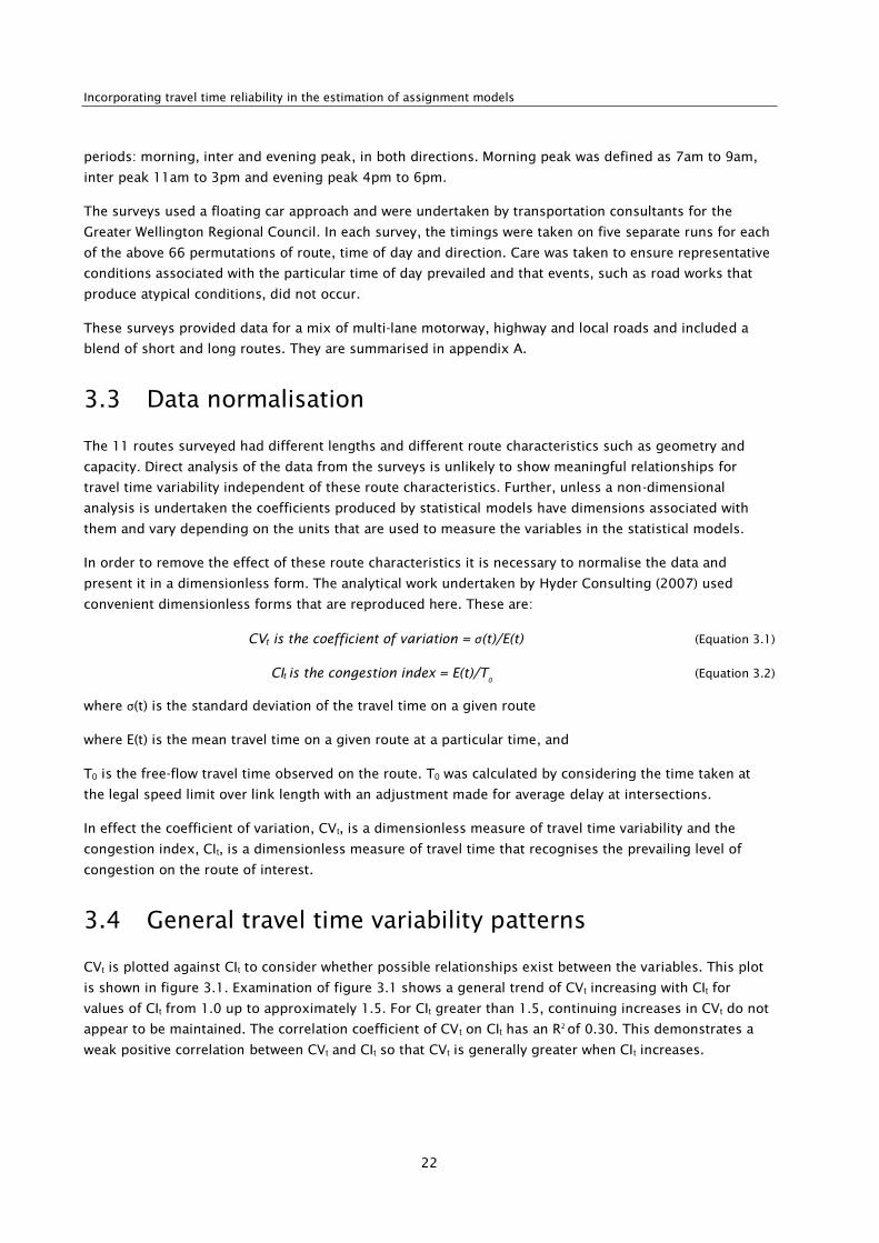
3.3 Data normalisation
The 11 routes surveyed had different lengths and different route characteristics such as geometry and
capacity. Direct analysis of the data from the surveys is unlikely to show meaningful relationships for
travel time variability independent of these route characteristics. Further, unless a non-dimensional
analysis is undertaken the coefficients produced by statistical models have dimensions associated with
them and vary depending on the units that are used to measure the variables in the statistical models.
In order to remove the effect of these route characteristics it is necessary to normalise the data and
present it in a dimensionless form. The analytical work undertaken by Hyder Consulting (2007) used
convenient dimensionless forms that are reproduced here. These are:
CVt is the coefficient of variation = σ(t)/E(t) (Equation 3.1)
CIt is the congestion index = E(t)/T0
(Equation 3.2)
where σ(t) is the standard deviation of the travel time on a given route
where E(t) is the mean travel time on a given route at a particular time, and
T0 is the free-flow travel time observed on the route. T0 was calculated by considering the time taken at
the legal speed limit over link length with an adjustment made for average delay at intersections.
In effect the coefficient of variation, CVt, is a dimensionless measure of travel time variability and the
congestion index, CIt, is a dimensionless measure of travel time that recognises the prevailing level of
congestion on the route of interest.
3.4 General travel time variability patterns
CVt is plotted against CIt to consider whether possible relationships exist between the variables. This plot
is shown in figure 3.1. Examination of figure 3.1 shows a general trend of CVt increasing with CIt for
values of CIt from 1.0 up to approximately 1.5. For CIt greater than 1.5, continuing increases in CVt do not
appear to be maintained. The correlation coefficient of CV t on CIt has an R2
of 0.30. This demonstrates a
weak positive correlation between CVt and CIt so that CVt is generally greater when CIt increases.

3 Data analysis
23
Figure 3.1 CV vs CI
If the points with CIt greater than 1.5 are treated as ‘outliers’ and removed then the distribution of points
shown in figure 3.2 is obtained. The value of CIt equal to 1.5 has been chosen from inspection of figure
3.1 but has been generalised in the analyses in later sections of this report.
Generally, these outliers relate to routes in or approaching central Wellington. The outliers occur in pairs –
one outlier at a location and traffic direction in the morning peak is matched by another at the same
location in the evening peak but in the opposite traffic direction.
Figure 3.2 shows a strong correlation between CVt and CIt and the correlation coefficient R2
has a value of
0.77. It would appear there is some evidence of a correlation between CVt and CIt which is strengthened if
the points with CIt greater than 1.5 are removed. As discussed in later sections this result is pointing to
two distinct flow phases where the phase transition occurs near CIt equal to 1.5. At lower values of CIt flow
becomes more variable as CIt increases and at higher values of CIt flow breaks down and travel times
become more certain but longer as CIt increases.
Another explanation may be contained in the findings of Arup (2004) who argued that in highly congested
situations the mean and standard deviation of travel time was dependent on the demand profile, including
that before the modelled period. When CIt is greater than 1.5 this means actual travel times are more than
50% greater than free-flow travel times which would suggest there is significant congestion.

Incorporating travel time reliability in the estimation of assignment models
24
Figure 3.2 CV vs CI outliers removed
3.5 Alternative measures of travel time reliability
Even though the concept of travel time reliability has not been as well developed as other areas of
transportation research, there was some mention of it in the literature. Lomax et al (2003) and Margiotta
(2002) discussed the use of standard statistical measures including mean travel time, the standard
deviation, variance and various percentile travel times. Their work represents some of the founding
thinking in the area of travel time reliability measurement.
The standard statistical measures of standard deviation, variance, percentile and the coefficient of
variation are related. The variance is the square of the standard deviation and, in the case of normally
distributed travel times, the 95th percentile travel time is approximately the mean travel time plus two
standard deviations. The coefficient of variation has been used here as a normalised form of the standard
deviation and is equal to the standard deviation divided by the mean travel time. These measures are
mathematically interchangeable.
Figures 3.3 and 3.4 show the standard deviation of travel time plotted against CIt and the variance plotted
against CIt. Both figures 3.3 and 3.4 have a significant outlier when CIt is approximately 1.37. The
respective standard deviation and variance is significantly greater than those for other values of CIt. These
outliers represent a measurement of travel time variability at the same location, time period and traffic
direction.

3 Data analysis
25
Figure 3.3 Standard deviation vs CI
The correlation coefficient R2
for the standard deviation plotted against CIt is 0.22 and the R2
for the
variance plotted against CIt is 0.06. These R2
values are inferior to those obtained for CVt plotted against CIt
and do not provide a compelling reason to adopt either the standard deviation or variance as the measure
of travel time variability.
When figures 3.3 and 3.4 are compared with figures 3.1 and 3.2 there are no obvious advantages in
directly using the standard deviation or the variance as the basis of the analysis. Further, the measures in
figures 3.3 and 3.4 are easily manipulated into the form used in figures 3.1 and 3.2. For these reasons it
is recommended that the dimensionless normalised form be used as the basis of further analysis.
3.6 Development of a travel time variability function using
the full data set
The following analysis uses the full data set presented in figure 3.1. In the next section an analysis is
undertaken where outliers are removed, as shown in figure 3.2.
A variety of models are investigated. These look at a wide range of potential functional relationships
between CVt and CIt. Of particular interest is the model of Hyder Consulting (2007) identified in the
literature review. This is of the form:
CVt
= αCIt
βdδ (Equation 3.3)
where CVt is the coefficient of variation = σ(t)/E(t)
where CIt is the congestion index = E(t)/T0

Incorporating travel time reliability in the estimation of assignment models
26
Figure 3.4 Variance vs CI
where d is route length in km
where T0 is the free-flow travel time for the route
and α, β and δ are constants that require calibrating
Equation 3.3 is mathematically equivalent to
ξ = ζ + βδ + δε (Equation 3.4)
where ξ = log10
(CVt)
where ζ = log10
(CIt)
where η = log10
(d)
and θ = log10
(α)
which is linear in form.
This means a functional form can be investigated where functions of log10(CIt) are analysed against
log10(CVt). There is no requirement to use logarithms to base 10 other than for convenience, as any
logarithmic base can be used. This includes the linearised form as in equation 3.4 above and more
complex alternatives.
The following models are investigated:
CVt = θ +βCIt (A)
ξ = θ + βζ (B)
ξ = θ + βζ + δη (C)
ξ = θ + βζ + δζ2
(D)
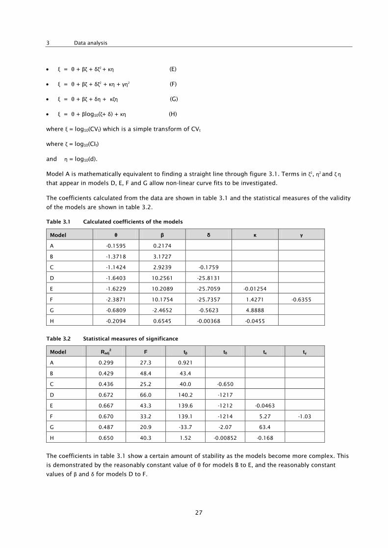
3 Data analysis
27
ξ = θ + βζ + δζ2
+ κη (E)
ξ = θ + βζ + δζ2
+ κη + γη2
(F)
ξ = θ + βζ + δη + κζη (G)
ξ = θ + βlog10(ζ+ δ) + κη (H)
where ξ = log10(CVt) which is a simple transform of CVt
where ζ = log10(CIt)
and η = log10(d).
Model A is mathematically equivalent to finding a straight line through figure 3.1. Terms in ζ2
, η2
and ζ η
that appear in models D, E, F and G allow non-linear curve fits to be investigated.
The coefficients calculated from the data are shown in table 3.1 and the statistical measures of the validity
of the models are shown in table 3.2.
Table 3.1 Calculated coefficients of the models
Model θ β δ κ γ
A -0.1595 0.2174
B -1.3718 3.1727
C -1.1424 2.9239 -0.1759
D -1.6403 10.2561 -25.8131
E -1.6229 10.2089 -25.7059 -0.01254
F -2.3871 10.1754 -25.7357 1.4271 -0.6355
G -0.6809 -2.4652 -0.5623 4.8888
H -0.2094 0.6545 -0.00368 -0.0455
Table 3.2 Statistical measures of significance
Model Radj2
F tβ tδ tκ tγ
A 0.299 27.3 0.921
B 0.429 48.4 43.4
C 0.436 25.2 40.0 -0.650
D 0.672 66.0 140.2 -1217
E 0.667 43.3 139.6 -1212 -0.0463
F 0.670 33.2 139.1 -1214 5.27 -1.03
G 0.487 20.9 -33.7 -2.07 63.4
H 0.650 40.3 1.52 -0.00852 -0.168
The coefficients in table 3.1 show a certain amount of stability as the models become more complex. This
is demonstrated by the reasonably constant value of θ for models B to E, and the reasonably constant
values of β and δ for models D to F.

Incorporating travel time reliability in the estimation of assignment models
28
These coefficients suggest CVt will generally increase with increasing CIt, but with the models that contain
quadratic terms, large values of CIt will allow a decline in CVt. It should be noted that a decrease in CVt
does not necessarily mean a decrease in the travel time variability, as measured by the standard deviation
of travel time, as CVt is the coefficient of variation equal to σ(t)/E(t). The coefficients suggest CVt will
generally decrease with increasing d. The above conclusions need to be qualified by the possibility there
may be some correlation between CIt and d.
In table 3.2 the Radj2
term, R2
adjusted for differing degrees of freedom, indicates models need to be fairly
complex before a reasonable fit is obtained as in models D, E, F and H. The F-statistics calculated for each
of the models A to H are statistically significant at both the 95% and 99% levels indicating all the models
have significant explanatory power.
The t-statistics for the various coefficients provide some useful insights. In the case of model A the
coefficient of CIt is not statistically significant at the 95% level. In models B to G the coefficients of ζ (ζ =
log10(CIt)) are statistically significant at both the 95% and 99% levels. In models D, E and F, which contain
terms in ζ2
, the coefficients are found to be significant at the 95% and 99% levels.
The t-statistics for coefficients of d and η (η = log10(d)) are not statistically significant at the 95% level
except in model F where the coefficient of η is statistically significant at both the 95% and 99% levels if a
quadratic term in η is included in the model.
These results suggest models D, E and F are the most promising.
3.7 Development of a travel time variability function with
outliers removed
The analysis in section 3.6 is repeated. This time it is assumed a number of points in figure 3.1 are
outliers and are distorting the analysis performed in section 3.6. This is because figure 3.1 appears to
show consistent trends for lower values of CIt but not for larger values. It may be that some other
relationships exist above a particular threshold in CIt. This is explained by road users responding to more
severe congestion in a way that is different from lower levels of traffic.
Such a possibility will be explored in this section. The outlier points are removed as in figure 3.2 and the
analysis presented in section 3.6 is repeated.
The results of this analysis are presented in tables 3.3 and 3.4.
Table 3.3 Calculated coefficients of the models with outliers removed
Model θ β δ κ γ
A -0.6594 0.6574
B -1.5619 6.8285
C -1.4756 6.6809 -0.06563
D -1.6964 11.6663 -28.0507
E -1.6426 11.4396 -27.2312 -0.03796
F -1.9757 11.4557 -27.5567 0.6470 -0.3179
G -1.0760 0.9671 -0.4007 5.1055
H 0.6045 1.5783 0.0302 -0.02982

3 Data analysis
29
Table 3.4 Statistical measures of significance with outliers removed
Model Radj2
F tβ tδ tκ tγ
A 0.772 193.2 5.11
B 0.748 169.6 149.8
C 0.747 84.7 146.6 -0.206
D 0.771 96.2 255.9 -3450
E 0.768 63.3 2509 -3349 -0.119
F 0.767 47.5 251.3 -3389 2.030 -0.460
G 0.781 68.5 21.2 -1.26 101.3
H 0.773 65.2 7.92 0.152 -0.0935
As in table 3.1, the coefficients shown in table 3.3 show some stability as the models become more
complex. This is demonstrated by the reasonably constant value of θ for models B to F, and the reasonably
constant values of β and δ for models D to F. These results show there is more stability when the outliers
are removed.
These coefficients suggest CVt will generally increase with increasing CIt, but with the models that contain
quadratic terms, larger values of CIt, will allow CVt to plateau and decrease. The coefficients suggest CVt
will generally decrease with increasing d. The above conclusions need to be qualified by the possibility
there may be some correlation between CIt and d.
In table 3.4, the Radj2
term indicates all the models show good fit. In particular the simple model A: CVt = θ
+βCIt, provides a good fit with only two coefficients. It is interesting to note that the two coefficients for
model A are closely related, with one being approximately the negative of the other.
This result suggests a model of the form CVt = β(CIt – 1) should be considered with β being approximately
0.658. Such a model has practical and theoretical appeal as it is simple in form, with just a single
coefficient, and easy to use for calculations. Further, such a model would suggest that under free-flow
conditions, where CIt = 1, the travel time variability would be zero. This property is consistent with
theoretical expectations.
If a relationship can be found between CVt and CIt using measured values of CVt and CIt, then this
relationship can be used to forecast unknown values of CVt
if traffic conditions change. An example of this
application includes measuring current patterns of CVt and CIt and asking what these might be in 20 years
time if traffic continues to grow with no changes to the network, or alternatively what CVt and CIt might be
if a road improvement or other measure is put in place. The F-statistics calculated for each of the models
A to H are statistically significant at both the 95% and 99% levels indicating the models have significant
explanatory power.
The t-statistics for the various coefficients provide some useful insights. In the case of model A the
coefficient of CIt is statistically significant at the 95% and 99% levels. In models B to G the coefficient of ζ (ζ
= log10(CIt)) is statistically significant at both the 95% and 99% levels. In model H the coefficient of log10(ζ)
is statistically significant at both the 95% and 99% levels. In models D, E and F, which contain terms in ζ2
,
the coefficients are found to be significant at the 95% and 99% levels.
The t-statistics for coefficients of d and η (η = log10(d)) are not found to be statistically significant at the
95% level except in model F where the coefficient of η is statistically significant at the 95% but not at the
99% level if a quadratic term in η is included in the model.

Incorporating travel time reliability in the estimation of assignment models
30
A comparison of table 3.2 with table 3.4 indicates that the removal of the outlier points generally
produces higher values of Radj2
. The values of the F-statistics in table 3.4 are generally larger than in table
3.2 indicating a higher level of statistical significance in the model. The t-statistics for the coefficients of ζ,
ζ 2
and log10(ζ) are generally larger in magnitude in table 3.4 than in table 3.2 indicating greater statistical
validity for the inclusion of these terms.
Neither table 3.2 nor table 3.4 provide statistical evidence for the validity of terms in d, η (η = log10(d)) and
η 2
. This result shows there is little statistical evidence to support models of the form of equation 3.3
developed by Hyder Consulting (2007) using data from the UK. There does not appear to be a clear reason
for this.
Figure 3.5 Non expressway CV vs CI
3.8 Development of a travel time variability function with
allowance for different types of roads
The question is posed as to whether the type of road may have an impact on travel time reliability.
Essentially the data set contains two types of roads: urban roads, and motorways and expressways. The
motorways and expressways are typically higher standard roads and are multi-laned with higher posted
speeds. They have few but well designed junctions. Urban roads frequently have single lane sections,
lower speed regimes, and a greater frequency and variety of junctions.
The analysis in section 3.6 is repeated, including the outlier points. This time the points in figure 3.1 are
separated into these two groups of roads and analysed separately. These data sets are presented in
figures 3.5 and 3.6.
The results of the analysis of urban roads that are not motorways or expressways are presented in tables
3.5 and 3.6.

3 Data analysis
31
Table 3.5 Calculated coefficients of the models for urban roads
Model θ β δ κ γ
A -0.2510 0.2965
B -1.4155 3.8938
C -1.3095 3.7126 -0.07880
D -1.7717 14.1670 -44.8777
E -1.7007 14.0155 -44.7374 -0.05191
F -1.3204 14.3629 -46.2103 -0.7948 0.3261
G -0.5698 -6.5224 -0.7631 10.4308
H -0.1898 0.7136 -0.00247 -0.00622
Figure 3.6 Expressway CV vs CI
As in tables 3.1 and 3.3, the coefficients in table 3.5 show some stability as the models become more
complex. This is demonstrated by the reasonably constant value of θ for models B to F, and the reasonably
constant values of β and δ for models D to F.
These coefficients suggest CVt will generally increase with increasing CIt, but with the models that contain
quadratic terms, larger values of CIt will allow CVt to plateau. The coefficients suggest CVt will generally
decrease with increasing d. The above conclusions need to be qualified by the possibility there may be
some correlation between CVt and d.
Table 3.6 Statistical measures of significance for urban roads
Model Radj2
F tβ tδ tκ tγ
A 0.373 27.4 1.33
B 0.470 40.9 60.8
C 0.462 20.3 58.0 -0.257

Incorporating travel time reliability in the estimation of assignment models
32
Model Radj2
F tβ tδ tκ tγ
D 0.709 56.5 221.2 -2953
E 0.704 37.1 218.9 -2944 -0.169
F 0.699 27.4 224.3 -3041 2.590 0.465
G 0.689 34.6 -101.8 -2.49 178.5
H 0.634 27.3 1.74 -0.00603 -0.0203
In table 3.6 the Radj2
term, indicates that models D to H show good fit and models A to C have a modest fit.
Generally the fits are better than those in table 3.2 where all the data is used but not as good as in table
3.4 where the outliers have been removed.
The F-statistics calculated for each of the models A to H are statistically significant at both the 95% and
99% levels indicating the models have significant explanatory power.
The t-statistics for the various coefficients provide some useful insights. In the case of model A the
coefficient of CIt is not statistically significant at the 95% level. In models B to G the coefficient of ζ (ζ =
log10(CIt)) is statistically significant at both the 95% and 99% levels. In model H the coefficient of log10(ζ) is
not statistically significant at the 95% level. In models D, E and F which contains terms in ζ 2
the coefficients
are found to be significant at the 95% and 99% levels.
The t-statistics for coefficients of d and η (η = log10(d)) are not found to be statistically significant at the
95% level except in model F where the coefficient of η is statistically significant at the 95% but not at the
99% level if a quadratic term in η is included in the model.
The t-statistics for the coefficients of ζ, ζ2
and log10(ζ) are generally larger in magnitude in table 3.6 than in
table 3.2 but not as large as those in table 3.4.
Table 3.6, as with tables 3.2 and 3.4, does not provide statistical evidence for the validity of terms in d, η
(η = log10(d)) and η2
. This result shows there is little statistical evidence to support models of the form of
equation 3.3 developed by Hyder Consulting (2007) using data from the UK.
The results of the analysis of motorways and expressways are presented in tables 3.7 and 3.8.
Table 3.7 Calculated coefficients of the models for motorways and expressways
Model θ β δ κ γ
A -0.05687 0.1313
B -1.3132 2.1325
C -0.5378 2.0182 -0.6219
D -1.5852 9.8814 -23.3098
E -0.9933 9.6389 -22.8406 -0.4704
F -1.1910 9.6389 -22.8406 -0.1456 -0.1322
G -1.3596 10.2548 0.04499 -6.8026
H 0.06557 0.4768 -0.00984 -0.3992

3 Data analysis
33
Table 3.8 Statistical measures of significance for motorways and expressways
Model Radj2
F tβ tδ tκ tγ
A 0.209 2.64 0.336
B 0.422 7.30 18.9
C 0.407 3.84 17.9 -5.21
D 0.763 16.4 87.5 -601.6
E 0.764 11.1 85.3 -589.5 -3.94
F 0.734 7.31 85.3 -589.5 -1.22 -0.451
G 0.406 2.82 90.8 0.377 -50.1
H 0.669 7.12 0.752 -0.0155 -3.35
Comparison of table 3.7 with table 3.1 shows similar patterns in the stability of the coefficients. The
coefficients of ζ and ζ 2
in table 3.7 are smaller in magnitude than those in table 3.5. This suggests
motorways and expressways have flatter curves when CVt is plotted against CIt.
Again table 3.7 suggests CVt increases with CIt although the coefficient of quadratic terms suggests this
may plateau or decrease with large values of CIt. The coefficients of terms involving distance indicate CVt
may decrease with increasing values of d.
Table 3.8 indicates the model fits are not particularly good for expressways and motorways. The values of
Radj2
are generally modest except with models D, E and F where terms in ζ 2
are used. The F-statistics
generally do not indicate a level of statistical significance in any of the models except for models E and F.
This is partly due to a small number of data points being available for expressways and motorways. In
models E and F, the F-statistics are significant at the 95% level but not at the 99% level.
The t-statistics of terms in ζ and ζ2
are statistically significant at the 95% and 99% levels. Other terms do
not generally have statistically significant t-statistics.
3.9 Extension of a simple linear travel time variability
function
In this section the simple linear model A of the form
CVt
= θ + βCIt
(Equation 3.5)
and the simpler theoretically more satisfying model
CVt = β(CIt – 1) (Equation 3.6)
are further developed.
Equation 3.5 and its special case represented by equation 3.6 have been determined by a least squares
regression fit where points from the data set where CIt is greater than 1.5 are removed as in figure 3.2.
The value of CIt where points with larger values are excluded is generalised to ψ.
Equation 3.5 is now used for all values of CIt and the difference between observed values of CVt and those
estimated by equation 3.5 are found. This difference is Δ(CVt). That is:

Incorporating travel time reliability in the estimation of assignment models
34
Δ(CVt
) = CVt
o
– (θ +βCIt
) (Equation 3.7)
where CVto
is the observed value of CVt.
Δ(CVt) is plotted against CIt in figure 3.7 and d in figure 3.8 for ψ = 1.5.
Figure 3.7 shows the expected collection of points with Δ(CVt) close to zero for CIt from 1.0 to 1.5. For CIt
greater than 1.5 there appears to be a monotonic decline in Δ(CVt) with increasing CIt. Figure 3.8 shows no
obvious relationship between Δ(CVt) and d.
Figure 3.7 Δ(CV) v CI
If ψ is allowed to vary away from 1.5 it is possible to find a value of ψ and models for CVt and Δ(CVt) that
give the best fit of the data. Such an analysis has been undertaken and the results for an optimal data fit
obtained using Radj2:
ψ = 1.395
CVt = -0.6714 + 0.6677CIt + Δ(CVt) (Equation 3.8)
where
Δ(CVt) = 0 CIt ≤ 1.395 (Equation3.9)
= 1.2306 – 0.8822CIt CIt > 1.395

3 Data analysis
35
Figure3.8 Δ(CV) vs distance d
The statistical measure of validity for these models is Radj2
=0.786 with the F-statistic being 118. This
measure indicates a good model fit for the complete data set, comparable with the results achieved for the
truncated data set used to produce table 3.4.
The t-statistic for the coefficient of CIt in equation 3.8 is 7.73, which is significant at both the 95% and 99%
levels. The t-statistic for the coefficient of CIt in equation 3.9 is –3.69, which is significant at both the 95%
and 99% levels.
The coefficients of equation 3.8 are again closely related and are approximately the form of equation 3.6
with β = 0.670.
The model for a travel time variability function represented by equations 3.8 and 3.9 appears to fit the
data well. The statistical measures of goodness of fit appear to support this model, as do the t-statistics of
the individual coefficients.

Incorporating travel time reliability in the estimation of assignment models
36
Figure 3.9 CV vs CI
The behaviour of this model for values of CIt greater than1.395 is consistent with figure 3.7. Equations 3.8
and 3.9 and figure 3.7, if accepted, would suggest CVt increases as traffic volumes increase above free-
flow conditions, but beyond a point (represented by CIt = 1.395) CVt would then decrease as traffic
volumes continue to increase.
In figure 3.9 this linear model is superimposed on top of the observed data. The model shows CVt increasing
up to the breakpoint as CIt increases and after the breakpoint CVt decreases as CIt continues to increase.
A second refinement is to investigate a linear functional relationship before the breakpoint with a
rectangular hyperbolic functional relationship following the breakpoint. The rectangular hyperbolic
relationship will prove mathematically convenient in the analysis later in this study. This is outlined in
equation 3.10.
CVt
= θ + βCIt
for CIt
≤ ψ (Equation 3.10)
= δ + κ/CIt
for CIt
≥ ψ
The coefficients θ, β, δ and κ are constrained so that CVt is continuous at CIt equal to ψ.
The optimum combination of these coefficients is given by:
θ = -0.7094, β = 0.7023, δ = -0.3105, κ =0.8465 with ψ = 1.418.
A relationship of the form of equation (3.6) where the constant θ is zero is given by equation 3.11.
CVt
= β(CIt
-1) for CIt
≤ ψ (Equation 3.11)
= δ + κ/CIt
for CIt
≥ ψ
The coefficients β, δ and κ are constrained so that CVt is continuous at CIt equal to ψ.

3 Data analysis
37
The optimum combination of these coefficients is given by:
β = 0.7058, δ = -0.3105, κ =0.8465 with ψ = 1.411.
The hyperbolic part of equation 3.11 cuts the horizontal axis at CIt equal to 2.726.
Figure 3.10 CV vs CI
Radj2
= 0.599, the F-statistic for the fit is 32.5 which is statistically significant at both the 95% and 99%
levels. The t-statistic for the coefficient β is 6.97 and κ is 10.8. These are both statistically significant at
the 95% and 99% levels. Again as with many of the earlier analyses θ approximately equals - β.
In figure 3.10 this linear-hyperbolic model is superimposed on top of the observed data. The model shows
CVt increasing linearly up to the breakpoint as CIt increases and after the breakpoint CVt decreases, this
time with a hyperbolic curve, as CIt continues to decrease.
A further refinement is to directly fit equation 3.6 and the more complex equation 3.12 to the data.
CVt
= β(CIt
– 1) + γ(CIt
– 1)2
(Equation 3.12)
Equation 3.12 is an extension of equation 3.6 and like equation 3.6 has the property that when CIt equals 1,
CVt is zero. However, the additional term, γ(CIt – 1)2
, allows a non linear curve fit and an extra degree of
freedom which may produce a better fit to the data.
The results of this refinement are provided in tables 3.9 and 3.10 for the optimum cut-off point for CIt of
1.49.

Incorporating travel time reliability in the estimation of assignment models
38
Figure 3.11 CV vs CI – 1
Table 3.9 Calculated coefficients of the models
Model β γ
CVt = β(CIt
– 1)
0.6650
CVt = β(CIt – 1)
+ γ(CIt – 1)2
0.5572 0.3323
Table 3.10 Statistical measures of significance
Model Radj2 F tβ tγ
CVt = β(CIt
– 1)
0.769 189.6 5.51
CVt = β(CIt – 1)
+ γ(CIt
–1)2
0.772 97.1 4.17 5.70
Figure 3.11 shows observed values of CVt plotted against CIt-1 with the linear and quadratic models from
tables 3.9 and 3.10 superimposed.
Both the linear (CVt = β(CIt – 1)) and quadratic (CVt = β (CIt – 1) + γ(CIt – 1)2
) models suggest travel time
variability will increase as route travel time and route congestion increase. The quadratic model suggests
the rate of increase of travel time variability will also increase with route travel time and route congestion
as the coefficient, γ, is positive.
The calculated value of Radj2
shows a good model fit for both the linear and the quadratic model. The Radj2
indicates the data fit for the quadratic model is better than the linear model but the amount of
improvement is only marginal. The F-statistics indicate the model fits are statistically significant at both
the 95% and 99% levels for both the linear and quadratic models. The t-statistics of all the coefficients of
both the linear and quadratic models are statistically significant at both the 95% and 99% levels.
Examination of figure 3.11, would suggest the values of CVt obtained from equations 3.6 and 3.12 are not
greatly different. This indicates that little benefit is achieved by adding the extra complexity implicit in
equation 3.12.

3 Data analysis
39
A useful result where a breakpoint, ψ, is identified in the behaviour of CVt causing it to monotonically
increase for values of CIt up to and including ψ and then monotonically decline for values of CIt greater
than ψ, is that the maximum value of CVt is calculated by:
maximum CVt = CVt(ψ) = β(ψ – 1) (Equation 3.13)
using the linear model and
maximum CVt
= CVt
(ψ) = β(ψ – 1) + γ(ψ – 1)2
(Equation 3.14)
using the quadratic model.
3.10 Implications of the linear, quadratic and hyperbolic
travel time variability functions
This section considers the mathematical implications of equations 3.6 and 3.12, and then equations 3.9
and 3.11. It looks in particular at the impact on travel time variability if the mean route travel time
changes. As discussed earlier, the mean route travel time may change for a variety of reasons, such as
ongoing traffic growth or the implementation of a road improvement.
3.10.1 Case 1: Both mean route travel times occur before the breakpoint
σ1 represents the travel time variability when the mean travel time is t1 and σ 2 represents the travel time
variability when the mean travel time is t2. Equations 3.1, 3.2 and 3.6 imply that:
(σ1
/ t1
)/(t1
/t0
–1) = β = (σ2
/ t2
)/(t2
/t0
–1) (Equation 3.15)
where both t1/t0 and t2/t0 are less than or equal to ψ which can be rewritten as both t1 and t2 are less than
or equal to ψt0; and β is the model coefficient, and in the case of the Wellington data used, is found to be
0.6650 and t0 is the route free-flow travel time.
Equation 3.15 can be rearranged to give:
σ2
/ σ1
= (t2
/ t1
).{( t2
- t0
)/( t1
- t0
)} (Equation 3.16)
Equation 3.16 enables the calculation of a new travel time variability directly from an old travel time
variability if the old, new mean and free-flow route travel times are known. This calculation does not
require the knowledge of the coefficient β in equation 3.6.
Equations 3.1, 3.2 and 3.12 can be rearranged to give:
σ2
/ σ1
= (t2
/ t1
).{[βt0
(t2
- t0
)+γ(t2
- t0
)2]
/[βt0
(t1
- t0
)+γ(t1
- t0
)2
]} (Equation 3.17)
As with equation 3.16, equation 3.17 allows the calculation of a new travel time variability from an old
travel time variability with the knowledge of the old, new and free-flow route travel times. Equation 3.17
requires the value of the coefficients β and γ to be known. This means, when using the quadratic model,
the new travel time reliability cannot be calculated from an old travel time reliability without knowledge of
β and γ. However, if using the linear model, knowledge of β is not required. Equations 3.16 and 3.17 are
valid, provided there is no break point ψ between the two values of CIt associated with t1 and t2.

Incorporating travel time reliability in the estimation of assignment models
40
3.10.2 Case 2: Both mean route travel times occur after the breakpoint
σ1 represents the travel time variability when the mean travel time is t1, and σ2 represents the travel time
variability when the mean travel time is t2. Using the linear model for values of CIt greater than ψ,
equations 3.8 and 3.9 can be written as:
CVt
= λ+ ωCIt (Equation 3.18)
Using algebraic manipulation equation 3.19 is obtained:
σ2
/ σ1
= (λt0
t2
+ ωt2
2
)/(λt0
t1
+ ωt1
2
) (Equation 3.19)
where both t1/t0 and t2/t0 are greater than or equal to ψ which can be rewritten as both t1 and t2 are greater
than or equal to ψt0.
If the hyperbolic model is used, as in equation 3.11, algebraic manipulation produces:
σ2
/ σ1
= (δt2
+ κt0
)/(δt1
+ κt0
) (Equation 3.20)
where, again, both t1/t0 and t2/t0 are greater than or equal to ψ which can be rewritten as both t1 and t2 are
greater than or equal to ψt0.
3.10.3 Case 3: The mean route travel times occur either side of the breakpoint
In this case the two mean travel times straddle the breakpoint. Using a linear model both before and after
the break point, algebraic manipulation produces:
σ2
/ σ1
= t2
(λt0
+ ωt2
)/(βt1
(t1
- t0
)2
) (Equation 3.21)
If the linear model is used before the breakpoint and the hyperbolic model is used after the breakpoint,
algebraic manipulation produces:
σ2
/ σ1
= t2
(δt0
+ κt2
)/(βt1
(t1
- t0
)2
) (Equation 3.22)
where t1/t0 is less than or equal to ψ and t2/t0 is greater than or equal to ψ. This can be rewritten as t1
being less than or equal to ψ t0 and t2 is greater than or equal to ψ t0.
For completeness, using the quadratic model before the breakpoint and the linear model after the
breakpoint produces equation 3.23, and using the quadratic model before the breakpoint and the
hyperbolic model after the breakpoint produces equation 3.24.
σ2
/ σ1
= t0
t2
(λt0
+ ωt2
)/(t1
(t1
- t0
)(βt0
+ γ(t1
- t0
))) (Equation 3.23)
σ2/
σ1
= t0
2
(δt2
+ κt0
)/(t1
(t1
- t0
)(βt0
+ γ(t1
- t0
))) (Equation 3.24)
where, again, t1/t0 is less than or equal to ψ and t2/t0 is greater than or equal to ψ. This can be rewritten
as t1 being less than or equal to ψt0 and t2 is greater than or equal to ψt0.
The models developed here are based on Wellington data. It is expected the coefficients obtained in other
places may be different. Further, the break points described by the parameter ψ required by equations 3.8
and 3.9 may also vary from location to location. If this is the case then these parameters will need to be
determined at each location. The advantage of equation 3.16 is that it is not reliant on determining these
coefficients and, as discussed in section 3.9, equation 3.17 is unlikely to provide a significantly different

3 Data analysis
41
estimate of σ2/ σ1 from the estimate obtained in equation 3.16. In the cases of equations 3.20 and 3.24
knowledge of these local coefficients is required.
3.11 Summary
Data from the 2007 travel time surveys in Wellington was useful for investigating travel time variability.
The data provided a mix of shorter and longer routes, local roads, highways and motorways, and two-lane
and multiple-lane roads.
The methodology of Hyder Consulting (2007) provided a convenient approach for data normalisation,
enabling travel time data to be converted into dimensionless variables.
Analysis of the travel time variability data appeared to show a relationship between travel time variability
and route mean travel time and therefore the congestion on the route. There did not appear to be a
relationship between travel time variability and route distance.
A variety of models were investigated to estimate travel time variability. When the total data set was used
the data fits were not good unless complex models were used. These models indicated relationships
existed between travel time variability and normalised route travel time but did not support a relationship
with route length. The coefficients of the normalised route travel time variables were generally found to be
statistically significant.
If data, where the route travel time was approximately 50% or greater than the free-flow route travel time,
was excluded then good data fits could be achieved with simple models of travel time variability. These
models did not support the inclusion of route travel distance. Simple refinements of these models
provided good data fit.
The analysis of the data by different models gave evidence that the relationship between CVt and CIt had
two distinct phases. In the first phase CVt monotonically increased with CIt and in the second phase CVt
monotonically decreased with CIt. The various models had a reasonably consistent breakpoint, ψ, where ψ
was approximately 1.4. It appeared this breakpoint indicated a point where traffic flow became so
congested the flow broke down. Increasing congestion beyond this breakpoint led to increasing delay but
the amount of delay was less uncertain.
Linear, quadratic and hyperbolic relationships between travel time variability and normalised route travel
time provided a mathematically simple approach to estimating travel time variability.
Further research would be helpful to demonstrate, or otherwise, the transferability of the relationships
obtained to other locations. In particular, it would be interesting to observe how the coefficients of the
models obtained in the above investigations changed in locations outside Wellington. This would include
identifying the value of the breakpoint represented by ψ in equations 3.8 and 3.9.
The breakpoint represented by ψ in equations 3.8 and 3.9 suggested the behaviour of CVt might undergo
some change with higher levels of congestion, possibly associated with some kind of change in the traffic
flow regime. This phenomenon should be examined further.

Incorporating travel time reliability in the estimation of assignment models
42
4 Application to a simple network
4.1 Preamble
The next stage of the project built upon the literature review and data analysis to consider how travel time
reliability might be incorporated into an assignment model and to test whether the effects of doing so
were statistically significant.
A simple hypothetical network created for this investigation was examined. However, the road link
attributes such as capacity, free-flow travel time and others were based on characteristics measured in the
model calibration phase of this study in Wellington. The travel time reliability function was derived from
the one calibrated for the Wellington network in the previous phase of this project.
Two assignment techniques were investigated. These were the deterministic ‘all or nothing’ and the logit
formulation. Each was examined for its suitability to incorporate travel time reliability and the effects of
doing so were identified. Techniques were identified to incorporate travel time reliability and
recommendations have been made.
4.2 Description of the network and trip matrices
The simple network developed had link characteristics similar to those found for the Wellington network in
the previous phase of this project.
The network is shown in figure 4.1 and has four nodes connected by five links. Each of the links is a two
lane two-way road. The characteristics of the road links are shown in table 4.1.
For the purposes of the investigation equation 4.1 is assumed to be the relationship between the
coefficient of variation of travel time and the congestion index. This equation has been derived from the
work in section 3.9 based on the analysis of data in Wellington.
CVt = σ/t = 0.7058(CI-1) CIt ≤ 1.4104 (Equation 4.1)
= -0.3105+0.8465/CIt CIt ≥ 1.4104 and ≤ 2.7262
= 0 CIt ≥ 2.7262
where CIt = t/t0 the congestion index
CVt is the coefficient of variation of link travel time
σ is the standard deviation of link travel time
t0 is the free-flow link travel time
t is the link travel time.
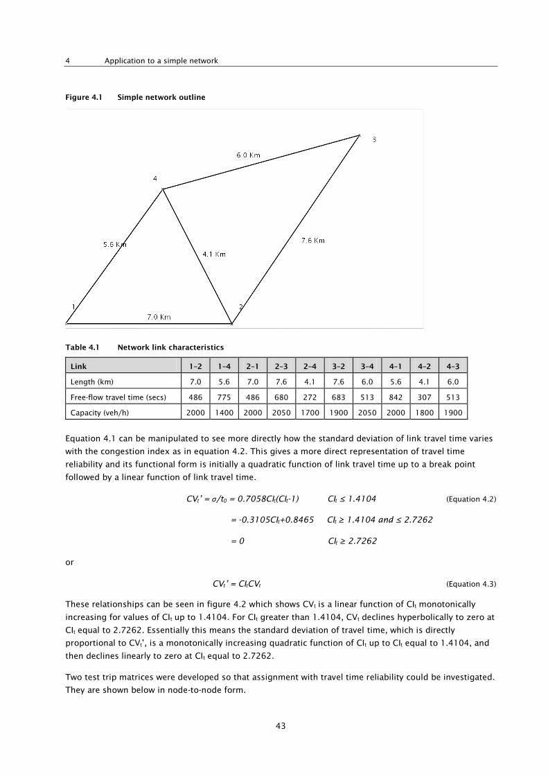
4 Application to a simple network
43
Figure 4.1 Simple network outline
Table 4.1 Network link characteristics
Link 1–2 1–4 2–1 2–3 2–4 3–2 3–4 4–1 4–2 4–3
Length (km) 7.0 5.6 7.0 7.6 4.1 7.6 6.0 5.6 4.1 6.0
Free-flow travel time (secs) 486 775 486 680 272 683 513 842 307 513
Capacity (veh/h) 2000 1400 2000 2050 1700 1900 2050 2000 1800 1900
Equation 4.1 can be manipulated to see more directly how the standard deviation of link travel time varies
with the congestion index as in equation 4.2. This gives a more direct representation of travel time
reliability and its functional form is initially a quadratic function of link travel time up to a break point
followed by a linear function of link travel time.
CVt’ = σ/t0 = 0.7058CIt(CIt-1) CIt ≤ 1.4104 (Equation 4.2)
= -0.3105CIt+0.8465 CIt ≥ 1.4104 and ≤ 2.7262
= 0 CIt ≥ 2.7262
or
CVt’ = CItCVt
(Equation 4.3)
These relationships can be seen in figure 4.2 which shows CVt is a linear function of CIt monotonically
increasing for values of CIt up to 1.4104. For CIt greater than 1.4104, CVt declines hyperbolically to zero at
CIt equal to 2.7262. Essentially this means the standard deviation of travel time, which is directly
proportional to CVt’, is a monotonically increasing quadratic function of CIt up to CIt equal to 1.4104, and
then declines linearly to zero at CIt equal to 2.7262.
Two test trip matrices were developed so that assignment with travel time reliability could be investigated.
They are shown below in node-to-node form.

Incorporating travel time reliability in the estimation of assignment models
44
Table 4.2 Trip matrix T1 (vehicles/h)
Origin/destination 1 2 3 4 Total
1 0 1550 250 400 2200
2 1500 0 450 4000 5950
3 300 450 0 375 1125
4 400 4000 375 0 4775
Total 2200 6000 1075 4775 14,050
Table 4.3 Trip matrix T2 (vehicles/h)
Origin/destination 1 2 3 4 Total
1 0 1550 1375 1250 4175
2 1500 0 1675 2500 5675
3 1420 1625 0 1280 4325
4 1250 2500 1175 0 4925
Total 4170 5675 4225 5030 19,100
T1 and T2 were chosen to provide a contrast in trip patterns. T1 has heavy demands in a selected number of
origins and destinations with the rest of the origins and destinations having light demands. T2 has less
contrast between the sizes of the origin destination pairs.
The leading diagonal of both T1 and T2 are all zeros. This is because we are only concerned with the
assignment of trips from zone to zone and the values of intra-zonal trips have no relevance.
Figure 4.2 CV vs CI

4 Application to a simple network
45
4.3 The effect of travel time reliability on link volumes
Trip matrices T1 and T2 can be assigned to the network shown in figure 4.1. Two assignment methods are
used. These are the ‘all or nothing’ and the logit formulation.
The trip matrix is assigned in increments. The all or nothing routine assigns all the trips for each origin-
destination pair in each increment to the lowest travel cost route. After each increment of the matrix has
been assigned the travel costs on any particular link are updated for the whole network and the next
increment of the trip matrix is assigned. This is continued until the whole trip matrix is assigned.
In the logit assignment process a similar approach is followed except that instead of all the trips of a
particular origin-destination pair being assigned to the lowest cost route, trips are assigned to alternative
route options using the logit formulation shown in equation 4.4.
Tk
ij = Tije-ζCk
/(∑g Tije-ζCg
) (Equation 4.4)
where Tij are the number of trips travelling between origin i and destination j
Tk
ij are the number of trips travelling between origin i and destination j using route k
θ is a factor used to convert travel costs to dis-utilities and
ck is the travel cost of using route k.
Applying either an all or nothing or a logit assignment routine is dependent, among other things, on the
determination of the route travel cost. A simple cost function is postulated as shown in equation 4.5 and
is of the form discussed in section 2.6.
ck = δdk + Τtk
+ ςσk (Equation 4.5)
where dk is the length of route k
tk is the travel time of route k
σk is the standard deviation of travel time on route k
δ,Τ and ς are perceived costs per unit distance, time and travel time reliability respectively.
Equation 4.5 is a simple generalisation of a perceived cost function used in many assignment models that
contains only travel distance and travel time. It is important to recognise that equation 4.5 represents
perceived costs and not actual costs. For example, road users do not understand the full costs associated
with distance. Typically wear- and tear-related costs are not consciously recognised. For the purposes of
the investigations that follow, typical values of δ and Τ have been adopted. These are $0.0875/km and
$16.27/hr respectively. In the work that follows ς will be varied to understand its effect with other values
held constant.
A simple spreadsheet model is used to do these assignments for both the all or nothing and logit
formulations. Speed flow curves are developed for each of the links as a function of traffic volume and link
capacity. The speed flow curves assume link travel time increases with the fourth power of the traffic
volume to capacity ratio and are calibrated to broadly approximate Wellington conditions. These speed
flow curves enable a value of tk to be calculated for each link at each incremental assignment.
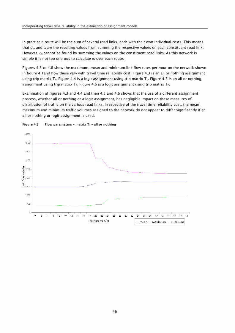
Incorporating travel time reliability in the estimation of assignment models
46
In practice a route will be the sum of several road links, each with their own individual costs. This means
that dk, and tk are the resulting values from summing the respective values on each constituent road link.
However, σk cannot be found by summing the values on the constituent road links. As this network is
simple it is not too onerous to calculate σk over each route.
Figures 4.3 to 4.6 show the maximum, mean and minimum link flow rates per hour on the network shown
in figure 4.1and how these vary with travel time reliability cost. Figure 4.3 is an all or nothing assignment
using trip matrix T1. Figure 4.4 is a logit assignment using trip matrix T1. Figure 4.5 is an all or nothing
assignment using trip matrix T2. Figure 4.6 is a logit assignment using trip matrix T2.
Examination of figures 4.3 and 4.4 and then 4.5 and 4.6 shows that the use of a different assignment
process, whether all or nothing or a logit assignment, has negligible impact on these measures of
distribution of traffic on the various road links. Irrespective of the travel time reliability cost, the mean,
maximum and minimum traffic volumes assigned to the network do not appear to differ significantly if an
all or nothing or logit assignment is used.
Figure 4.3 Flow parameters – matrix T1 – all or nothing

4 Application to a simple network
47
Figure 4.4 Flow parameters – matrix T1 – logit
Figure 4.5 Flow parameters – matrix T2 – all or nothing
If figures 4.3 and 4.4 are compared to figures 4.5 and 4.6 it can be seen the former show a greater
response to increasing travel time reliability cost than figures 4.5 and 4.6. It would appear that trip
matrices where there is a dominance of certain movements over the remainder of the trip movements,
subject to the overall volume of trips, would be more responsive to increasing travel time reliability cost.
In figures 4.3 to 4.6 there is little change in the maximum, mean and minimum link flow values for low
values of travel time reliability cost. However, in figures 4.3 and 4.4 once the travel time reliability cost
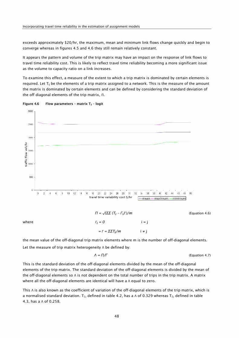
Incorporating travel time reliability in the estimation of assignment models
48
exceeds approximately $20/hr, the maximum, mean and minimum link flows change quickly and begin to
converge whereas in figures 4.5 and 4.6 they still remain relatively constant.
It appears the pattern and volume of the trip matrix may have an impact on the response of link flows to
travel time reliability cost. This is likely to reflect travel time reliability becoming a more significant issue
as the volume to capacity ratio on a link increases.
To examine this effect, a measure of the extent to which a trip matrix is dominated by certain elements is
required. Let Tij be the elements of a trip matrix assigned to a network. This is the measure of the amount
the matrix is dominated by certain elements and can be defined by considering the standard deviation of
the off diagonal elements of the trip matrix, Π.
Figure 4.6 Flow parameters – matrix T2 – logit
Π = √(∑∑ (Tij – Γij)2
)/m (Equation 4.6)
where Γij = 0 i = j
= Γ = ∑∑Tij/m i ≠ j
the mean value of the off-diagonal trip matrix elements where m is the number of off-diagonal elements.
Let the measure of trip matrix heterogeneity Λ be defined by:
Λ = Π/Γ (Equation 4.7)
This is the standard deviation of the off-diagonal elements divided by the mean of the off-diagonal
elements of the trip matrix. The standard deviation of the off-diagonal elements is divided by the mean of
the off-diagonal elements so Λ is not dependent on the total number of trips in the trip matrix. A matrix
where all the off-diagonal elements are identical will have a Λ equal to zero.
This Λ is also known as the coefficient of variation of the off-diagonal elements of the trip matrix, which is
a normalised standard deviation. T1, defined in table 4.2, has a Λ of 0.329 whereas T2, defined in table
4.3, has a Λ of 0.258.

4 Application to a simple network
49
As there are 12 off-diagonal elements in T1 and T2 there is a large number of ways the elements of these
matrices can be varied each with a consequential value of Λ. To get an understanding of the impact of
matrix heterogeneity just the movements between nodes 2 and 4 are varied so a consistent trend can be
developed. These have been selected as they are the clearest examples of movements whose magnitudes
are at a scale different from the remainder of the trip movements.
Figure 4.7 shows the spread of traffic assigned to the various links of the network expressed as a range
and standard deviation of link traffic volumes versus trip matrix heterogeneity for a travel time reliability
cost of $16.27/hr.
It can be seen from figure 4.7 that the range and standard deviation of link traffic volumes are highly non-
linear with respect to matrix heterogeneity. The spread of traffic assigned across the network is generally
greater with more heterogeneous trip matrices.
Figure 4.7 Range and standard deviation of link traffic volumes vs matrix heterogeneity
However, this spread of traffic across the network does not monotonically increase with trip matrix
heterogeneity. This is because the travel costs of alternative routes may become more attractive with
higher volumes of traffic. It might be expected with more complex networks that the effects of any
particular alternative route becoming more attractive in terms of travel cost will be less significant and so
the range and standard deviation of traffic assigned to the links of the network might appear to increase
more smoothly.
The range and standard deviation of traffic volumes assigned across the network is illustrated further by
examination of figures 4.8 and 4.9.

Incorporating travel time reliability in the estimation of assignment models
50
Figure 4.8 Variance of link volumes vs travel time reliability cost – matrix T1
Figure 4.9 Variance of link volumes vs travel time reliability cost – matrix T2
Figure 4.8 shows the range and standard deviation of traffic distributed across the network links for
matrix T1, which is a trip matrix with heterogeneity of 0.329 (showing high dominance by certain trip
movements). Figure 4.9 shows the same plot but this time for trip matrix T2, which is a trip matrix of
heterogeneity 0.258 (showing little dominance by any trip movements).
It can be seen from these plots that large values of travel time reliability cost have a significant impact on
heterogeneous trip matrices that reduces the range and standard deviation of traffic assigned to the
network. This makes the distribution of traffic across the various links more uniform. With fewer

4 Application to a simple network
51
heterogeneous trip matrices the effect is less pronounced. In simple terms, as people value travel time
reliability more they are more inclined to seek alternative routes where reliability may be greater. However,
a less heterogeneous trip matrix means traffic volumes are typically more evenly spread across the
network reducing the likelihood of any one route being much more congested than another. This reduces
the incentive to use alternative routes.
4.4 Measures of assignment validation
Equation 4.7 provides a means of incorporating travel time reliability into the assignment of traffic onto a
network. To do this there needs to be a way of determining the travel time reliability cost parameter ς.
One approach is to use a value of ς determined from willingness to pay surveys. For example Margiotta
(2006) undertook investigations that indicated the willingness to pay for reduced travel time variability
was two to six times that of willingness to accept a reduced mean travel time. However, it has been found
in assignment models that road users respond to a perceived travel distance cost rather than an actual
travel distance cost in their route choice decisions.
An approach that recognises this is to examine route choice decisions and select a value of ς that
optimises the assignment model fit. In order to do this, measures of model validation need to be
considered.
Three measures of model validation are in common use. The first examines the correlation coefficient R2
for link volumes from the model with observed traffic volumes. The second uses the root-mean-square-
error measure and the final measure involves GEH statistics.
The correlation coefficient R2
compares the model assigned link volumes with actual observed volumes.
The NZTA (2010) Economic evaluation manual requires the correlation coefficient R2
to be at least 0.85
overall and 0.95 in the vicinity of any scheme being investigated for acceptable validation. Hence, the
optimal choice of ς is one that maximises R2
.
The root-mean-square-error measure calculates the statistic:
%RMSE = 100 √∑((vobs – vmod)2
/ (n-1))/(∑vmod/n) (Equation 4.8)
where vobs is the observed link volume
vmod is the modelled link volume
n is the number of road links
and the summation is carried out over all n road links. For acceptable validation the Economic evaluation
manual requires the %RMSE to be 30 or less. Hence, the optimal choice of ς is one that minimises %RMSE.
In essence the root-mean-square-error measure is a modified form of a chi-squared test.
GEH statistics are calculated for individual road links in accordance to
GEH =√((2(vmod – vobs)2
/(vmod + vobs)) (Equation 4.9)
The Economic evaluation manual (NZTA 2010) requires that, for an acceptable level of validation:
60% of the links in the network have GEH < 5.0

Incorporating travel time reliability in the estimation of assignment models
52
95% of GEH < 10.0
100% of GEH < 12.0.
As this link-by-link approach is not convenient for the problem of choosing a ς that optimises validation it
is proposed to define a modified GEH that examines the whole network at once. This statistic is the root-
mean-squared-GEH defined by:
RMGEH2
= √(∑GEHi2
) (Equation 4.10)
where GEHi is the GEH from equation 4.9 calculated for the ith road link. In essence RMGEH2
is the
magnitude of the n dimensional vector whose ith element is the GEH statistic for the ith road link and n is
the number of road links. Hence, the optimal choice of ς is one that minimises RMGEH2
. Again, RMGEH2
is
a modified chi-squared test.
In the investigations that followed, each of these measures was examined to see whether they were useful
in determining whether a validation was improved by incorporating travel time reliability. It may be that a
validation is so flawed that incorporating travel time reliability shows an improvement in the validation.
4.5 Validation tests
A series of experiments assigned matrices T1 and T2 to the network shown in figure 4.1. A selection of
observed traffic volumes was assumed for the tests, which included all or nothing and logit based
assignments. These observed flows were chosen to ensure a range of ς results that optimised the
validations. This was done to get a greater understanding of the influence of ς. The inputs into these tests
are summarised in appendix B.
In each test ς was allowed to vary and the resulting R2
, %RMSE and RMGEH2
were calculated. This allowed the
identification of ς that approximately optimised each of R2
, %RMSE and RMGEH2
for each test. There was no
reason to believe that each of R2
, %RMSE and RMGEH2
would have the same value of ς for an optimum value.
The attributes of the tests are shown in table 4.4.
Table 4.4 Experiment attributes
E1 E2 E3 E4 E5 E6 E7 E8
Matrix T1
T1
T2
T2 T1 T1 T2 T2
Assignment all or
nothing
all or
nothing
all or
nothing
all or
nothing
logit logit logit logit
The experiments with the attributes summarised in table 4.4 occurred in pairs. This allowed two sets of
observed link flows to be tested for each matrix and assignment process.
4.5.1 Experiment E1
A graph of R2
, %RMSE and RMGEH2
with travel time reliability cost ς is shown in figure 4.10 for experiment
E1. This is the assignment of a trip matrix with high heterogeneity, T1, using an all or nothing assignment.
From figure 4.10 it can be seen that initially increasing travel time reliability cost ς does not improve
validation significantly. It is not until the travel time reliability cost exceeds $14/hr that the three
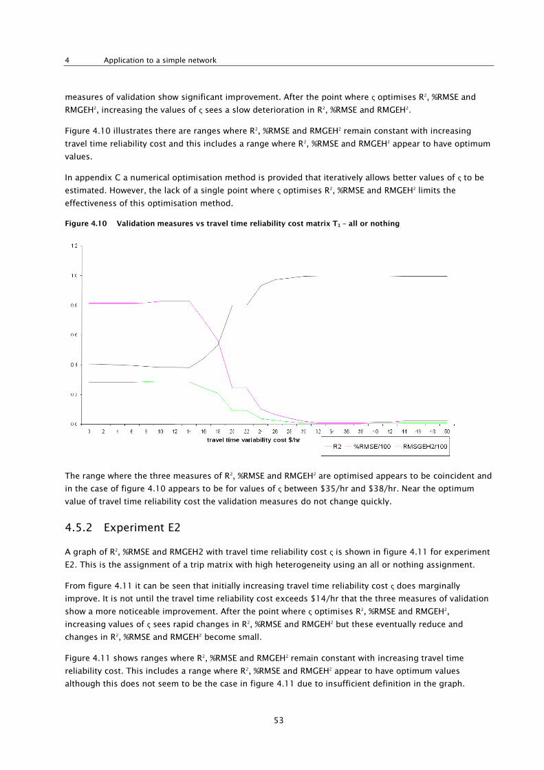
4 Application to a simple network
53
measures of validation show significant improvement. After the point where ς optimises R2
, %RMSE and
RMGEH2
, increasing the values of ς sees a slow deterioration in R2
, %RMSE and RMGEH2
.
Figure 4.10 illustrates there are ranges where R2
, %RMSE and RMGEH2
remain constant with increasing
travel time reliability cost and this includes a range where R2
, %RMSE and RMGEH2 appear to have optimum
values.
In appendix C a numerical optimisation method is provided that iteratively allows better values of ς to be
estimated. However, the lack of a single point where ς optimises R2
, %RMSE and RMGEH2
limits the
effectiveness of this optimisation method.
Figure 4.10 Validation measures vs travel time reliability cost matrix T1 – all or nothing
The range where the three measures of R2
, %RMSE and RMGEH2
are optimised appears to be coincident and
in the case of figure 4.10 appears to be for values of ς between $35/hr and $38/hr. Near the optimum
value of travel time reliability cost the validation measures do not change quickly.
4.5.2 Experiment E2
A graph of R2
, %RMSE and RMGEH2 with travel time reliability cost ς is shown in figure 4.11 for experiment
E2. This is the assignment of a trip matrix with high heterogeneity using an all or nothing assignment.
From figure 4.11 it can be seen that initially increasing travel time reliability cost ς does marginally
improve. It is not until the travel time reliability cost exceeds $14/hr that the three measures of validation
show a more noticeable improvement. After the point where ς optimises R2
, %RMSE and RMGEH2
,
increasing values of ς sees rapid changes in R2
, %RMSE and RMGEH2
but these eventually reduce and
changes in R2
, %RMSE and RMGEH2
become small.
Figure 4.11 shows ranges where R2
, %RMSE and RMGEH2
remain constant with increasing travel time
reliability cost. This includes a range where R2
, %RMSE and RMGEH2
appear to have optimum values
although this does not seem to be the case in figure 4.11 due to insufficient definition in the graph.

Incorporating travel time reliability in the estimation of assignment models
54
Figure 4.11 Validation measures vs travel time reliability cost – matrix T1 – all or nothing
The lack of a single point where ς optimises R2
, %RMSE and RMGEH2
limits the effectiveness of the
optimisation method provided in appendix C.
The range where the three measures of R2
, %RMSE and RMGEH2
are optimised appears to be coincident and
in the case of figure 4.11 appears to be for values of ς in the vicinity of $16/hr. Near the optimum value of
travel time reliability cost the validation measures change quickly.
4.5.3 Experiment E3
A graph of R2
, %RMSE and RMGEH2
with travel time reliability cost ς is shown in figure 4.12 for experiment
E3. This is the assignment of a trip matrix with low heterogeneity using an all or nothing assignment.
From figure 4.12 it can be seen that initially increasing travel time reliability cost ς does not improve
validation significantly. It is not until the travel time reliability cost exceeds $3/hr, which is a low value of
travel time reliability cost, that the three measures of validation show significant improvement. Again R2
,
%RMSE and RMGEH2
remain constant until the travel time reliability cost reaches approximately $24/hr
where a second improvement in R2
, %RMSE and RMGEH2
occurs. After the point where ς optimises R2
,
%RMSE and RMGEH2
, increasing values of ς sees steady deterioration in R2
, %RMSE and RMGEH2
, which
occurs through a series of steps.
Figure 4.12 also shows ranges where R2
, %RMSE and RMGEH2
remain constant with increasing travel time
reliability cost. This includes a range where R2
, %RMSE and RMGEH2
appear to have optimum values.

4 Application to a simple network
55
Figure 4.12 Validation measures vs travel time reliability cost – matrix T2 – all or nothing
The lack of a single point where ς optimises R2
, %RMSE and RMGEH2
limits the effectiveness of the
optimisation method provided in appendix C.
The range where the three measures of R2
, %RMSE and RMGEH2
are optimised appears to be coincident and
in the case of figure 4.12 appears to be for values of ς in the range of $23/hr to $39/hr. Near the
optimum value of travel time reliability cost the validation measures change slowly.
4.5.4 Experiment E4
A graph of R2
, %RMSE and RMGEH2
with travel time reliability cost ς is shown in figure 4.13 for experiment
E4. This is the assignment of a trip matrix with low heterogeneity using an all or nothing assignment.
From figure 4.13 it can be seen that initially increasing travel time reliability cost ς does not improve
validation significantly. It is not until the travel time reliability cost exceeds $3/hr that the three measures
of validation show significant improvement. It would appear this is a threshold at which one or more trip
movements switch route using the all or nothing assignment, and significantly improves validation. After
the point where ς optimises R2
, %RMSE and RMGEH2
increasing values of ς sees deterioration in R2
, %RMSE
and RMGEH2
which occur through a series of steps.
Figure 4.13 also shows ranges where R2
, %RMSE and RMGEH2
remain constant with increasing travel time
reliability cost. This includes a range where R2
, %RMSE and RMGEH2
appear to have optimum values.
The lack of a single point where ς optimises R2
, %RMSE and RMGEH2
limits the effectiveness of the
optimisation method provided in appendix C.

Incorporating travel time reliability in the estimation of assignment models
56
Figure 4.13 Validation measures vs travel time reliability cost – matrix T2 – all or nothing
The range where the three measures of R2
, %RMSE and RMGEH2
are optimised appears to be coincident and
in the case of figure 4.13 appears to be for values of ς in the range of $9/hr to $15/hr. Near the optimum
value of travel time reliability cost the validation measures change slowly.
4.5.5 Experiment E5
A graph of R2
, %RMSE and RMGEH2
with travel time reliability cost ς is shown in figure 4.14 for experiment
E5. This is the assignment of a trip matrix with high heterogeneity using a logit assignment.
From figure 4.14 it can be seen that initially increasing travel time reliability cost ς does not improve
validation. It is not until the travel time reliability cost exceeds $14/hr that the three measures of
validation show significant improvement. After the point where ς optimises R2
, %RMSE and RMGEH2
increasing values of ς sees a slow deterioration in R2
, %RMSE and RMGEH2
.
Figure 4.14 illustrates that R2
, %RMSE and RMGEH2
continue to vary, albeit slowly in some situations, with
increasing travel time reliability cost. This behaviour is different from that encountered with the all or
nothing assignment where in some ranges R2
, %RMSE and RMGEH2
remain constant.
In appendix C a numerical optimisation method is provided that iteratively allows better values of ς to be
estimated. Because the logit assignment provides a smooth curve this numerical method can be used to
calculate point where ς optimises R2
, %RMSE and RMGEH2
. However, figure 4.14 shows local optima exist
that are not the global optimum and so this method must be applied carefully to ensure the procedure
converges to the global optimum and not a local optimum.

4 Application to a simple network
57
Figure 4.14 Validation measures vs travel time reliability cost – matrix T1 – logit
The three measures of R2
, %RMSE and RMGEH2
are optimised at a value of ς which is approximately the
same for each of R2
, %RMSE and RMGEH2
. However, the optimum values of ς are not exactly coincident.
This experiment shows the curvature in %RMSE is the greatest of the three measures near the optimum
point and is the easiest in which to calculate the optimum point. The optimum point for ς for %RMSE is
$33.95/hr. Near the optimum value of travel time reliability cost the validation measures do not change
quickly.
4.5.6 Experiment E6
A graph of R2
, %RMSE and RMGEH2
with travel time reliability cost ς is shown in figure 4.15 for experiment
E6. This is the assignment of a trip matrix with high heterogeneity using a logit assignment.
From figure 4.15 it can be seen that initially increasing travel time reliability cost ς does not improve
validation until a travel time reliability cost of $14/hr is reached. After the point where ς optimises R2
,
%RMSE and RMGEH2
increasing values of ς sees steady deterioration in R2
, %RMSE and RMGEH2
but this
eventually plateaus.
Figure 4.15 illustrates that R2
, %RMSE and RMGEH2
continues to vary, albeit slowly in some situations, with
increasing travel time reliability cost. This behaviour is different from that encountered with the all or
nothing assignment where ranges were encountered where R2
, %RMSE and RMGEH2
remained constant.
In appendix C a numerical optimisation method is provided that iteratively allows better values of ς to be
estimated. Because the logit assignment provides a smooth curve this numerical method can be used to
calculate the point where ς optimises R2
, %RMSE and RMGEH2
. However, figure 4.15 shows local optima
exist which are not the global optimum and so this method must be applied carefully to ensure the
procedure converges to the global optimum and not a local optimum.

Incorporating travel time reliability in the estimation of assignment models
58
Figure 5.15 Validation measures vs travel time reliability cost – matrix T1 - logit
The three measures of R2
, %RMSE and RMGEH2
are optimised at a value of ς that is approximately the same
for each. However, the optimum values of ς are not exactly coincident. This experiment shows the
curvature in %RMSE is the greatest of the three measures near the optimum point and is the easiest in
which to calculate the optimum point. The optimum point for ς for %RMSE is $17.05/hr. Near the optimum
value of travel time reliability cost the validation measures change quickly.
4.5.7 Experiment E7
A graph of R2
, %RMSE and RMGEH2
with travel time reliability cost ς is shown in figure 4.16 for experiment
E7. This is the assignment of a trip matrix with low heterogeneity using a logit assignment.
From figure 4.16 it can be seen that initially increasing travel time reliability cost ς does improve
validation. After the point where ς optimises R2
, %RMSE and RMGEH2
, increasing values of ς sees steady
deterioration in R2
, %RMSE and RMGEH2
but this eventually plateaus.
Figure 4.16 illustrates that R2
, %RMSE and RMGEH2
continue to vary, albeit slowly in some situations, with
increasing travel time reliability cost. This behaviour is different from that encountered with the all or
nothing assignment where ranges were encountered where R2
, %RMSE and RMGEH2
remained constant.
In appendix C a numerical optimisation method is provided that iteratively allows better values of ς to be
estimated. Because the logit assignment provides a smooth curve this numerical method can be used to
calculate the point where ς optimises R2
, %RMSE and RMGEH2
. However, figure 4.16 shows local optima
exist which are not the global optimum and so this method must be applied carefully to ensure the
procedure converges to the global optimum and not a local optimum.

4 Application to a simple network
59
Figure 5.16 Validation measures vs travel time reliability cost – matrix T2 – logit
The three measures of R2
, %RMSE and RMGEH2
are optimised at a value of ς that is approximately the same
for each of R2
, %RMSE and RMGEH2
. However, the optimum values of ς are not exactly coincident. This
experiment shows the curvature in %RMSE is the greatest of the three measures near the optimum point
and is the easiest in which to calculate the optimum point. The optimum point for ς for %RMSE is
$38.29/hr. Near the optimum value of travel time reliability cost the validation measures change slowly.
4.5.8 Experiment E8
A graph of R2
, %RMSE and RMGEH2
with travel time reliability cost ς is shown in figure 4.17 for experiment
E8. This is the assignment of a trip matrix with low heterogeneity using a logit assignment.
From figure 4.17 it can be seen that initially increasing travel time reliability cost ς does improve
validation. After the point where ς optimises R2
, %RMSE and RMGEH2
, increasing values of ς sees steady
deterioration in R2
, %RMSE and RMGEH2
but this eventually plateaus.
Figure 4.17 illustrates that R2
, %RMSE and RMGEH2
continue to vary, albeit slowly in some situations, with
increasing travel time reliability cost. This behaviour is different from that encountered with the all or
nothing assignment where ranges were encountered where R2
, %RMSE and RMGEH2
remained constant.
In appendix C a numerical optimisation method is provided that iteratively allows better values of ς to be
estimated. Because the logit assignment provides a smooth curve this numerical method can be used to
calculate the point where ς optimises R2
, %RMSE and RMGEH2
. However, figure 4.17 shows local optima
exist which are not the global optimum and so this method must be applied carefully to ensure the
procedure converges to the global optimum and not a local optimum.

Incorporating travel time reliability in the estimation of assignment models
60
Figure 4.17 Validation measures vs travel time reliability cost – matrix T2 – logit
The three measures of R2
, %RMSE and RMGEH2
are optimised at a value of ς that is approximately the same
for each of R2
, %RMSE and RMGEH2
. However, the optimum values of ς are not exactly coincident. This
experiment shows the curvature in %RMSE is the greatest of the three measures near the optimum point
and is the easiest in which to calculate the optimum point. The optimum point for ς for %RMSE is
$13.09/hr. Near the optimum value of travel time reliability cost the validation measures change slowly
meaning nearby values of the validation statistics are only marginally worse.
4.5.9 Results summary
Experiments E1 to E8 had a broad range of characteristics. Four of the experiments used an all or nothing
assignment routine and the other four used a logit assignment. Two different trip matrices were used with
one having low heterogeneity and the other having high heterogeneity. Eight different ‘observed’ link
flows were used which broadly corresponded to a selection of travel time reliability costs that were small
and a selection that was large.
From the eight experiments above the following results were observed:
the all or nothing assignment produced a set of validation measures that were not a smooth function
of travel time reliability cost but contained a series of steps
the all or nothing assignment might not produce a discrete value of travel time reliability cost to
optimise the validation measures
the optimum value of travel time reliability cost for each validation measured R2
, %RMSE and RMGEH2
with an all or nothing assignment appearing to be in the same range
the logit assignment produced a set of validation measures that were a smooth function of travel time
reliability cost

4 Application to a simple network
61
the logit assignment produced similar results for the travel time reliability cost that optimised the
validation measures
the optimum value for each validation measure for logit assignment was approximately coincident
the validation measures each had more than one local point with a zero gradient so care had to be
taken to ensure the correct value of travel time reliability cost was chosen for optimising the various
validation measures
trip matrices with high heterogeneity showed slow response in the validation measures with small
travel time reliability costs
trip matrices with low heterogeneity showed rapid response in the validation measures with small
travel time reliability costs
all trip matrices showed slow response in the validation measures with large travel time reliability
costs
trip matrices with high heterogeneity showed slow change in the validation measures near the
optimum value of travel time reliability costs
trip matrices with low heterogeneity rapidly changed in the validation measures near the optimum
value of travel time reliability cost
of the three validation measures R2
, %RMSE and RMGEH2
, the measure %RMSE gave the sharpest
definition of the optimum value of travel time reliability cost with logit assignments.
These results are summarised in table 4.5 below.
Table 4.5 Experiment results
E1 E2 E3 E4 E5 E6 E7 E8
Matrix T1
T1
T2
T2 T1 T1 T2 T2
Assignment all or
nothing
all or
nothing
all or
nothing
all or
nothing
logit logit logit logit
Validation measure
form
not
smooth
not
smooth
not
smooth
not
smooth
smooth smooth smooth smooth
Response to small
travel time cost
slow slow rapid rapid slow slow rapid rapid
Response to large
travel time cost
slow slow slow slow slow slow slow slow
Response near
optimum value
slow slow rapid rapid slow slow rapid rapid
4.6 Statistical significance of improved validation by
including travel time reliability
In this section the statistical significance of improved validation of including travel time reliability is tested
using the results of the experiments in the previous section. This is done by testing the statistical

Incorporating travel time reliability in the estimation of assignment models
62
significance of the difference in the validation measure when the travel time reliability cost is zero and
optimum.
4.6.1 The correlation coefficient R2
Elementary college statistical theory teaches that the difference in the transformation, ξ, of the correlation
coefficient R2
given by equation 4.11 is approximately normally distributed.
ξ = 0.5loge((1 + R)/(1 - R)) (Equation 4.11)
Examination of table 4.6 shows the value of the transformed correlation coefficient for the optimum R2
,
ξopt, is significantly different from the value when travel time reliability cost is zero, at both the 95% and
99% levels. This was found to be the case for all eight experiments E1 to E8.
Table 4.6 Statistical significance of R2
E1 E2 E3 E4 E5 E6 E7 E8
R02
0.406 0.972 0.583 0.934 0.400 0.906 0.587 0.946
Ropt2
0.999 1.000 1.000 1.000 0.999 1.000 1.000 1.000
ξ0 0.754 2.468 1.005 2.067 0.745 1.849 1.011 2.141
ξopt
4.153 4.594 5.868 5.195 4.118 5.769 6.502 4.975
ξ95
3.499 3.941 5.215 4.541 3.465 5.116 5.849 4.321
ξ99
3.294 3.735 5.009 4.336 3.259 4.910 5.643 4.116
4.6.2 The root-mean-square-error %RMSE
The test of statistical significance of the difference in %RMSE when %RMSE is optimised and the travel time
reliability cost is zero assumes %RMSE is approximately normally distributed. A sample standard deviation of
%RMSE is calculated by using all the values calculated for travel time reliability cost equal to zero to $50/hr,
in integer increments, for each experiment. The results of this analysis are shown in table 4.7.
Table 4.7 Statistical significance of %RMSE
E1 E2 E3 E4 E5 E6 E7 E8
%RMSE0
81.623 18.484 11.966 5.707 81.896 31.601 11.964 5.501
%RMSEopt
1.110 2.150 0.118 0.171 1.049 0.628 0.052 0.270
%RMSE95
15.302 9.545 1.497 1.411 15.235 5.565 1.314 1.424
%RMSE99
19.763 11.870 1.930 1.801 19.693 7.117 1.710 1.787
Examination of table 4.7 shows when the value of %RMSE is optimised, %RMSEopt, it is sufficiently different
from the value when travel time reliability cost is zero to be statistically significant at both the 95% and
99% levels. This was found to be the case for all eight experiments E1 to E8.
4.6.3 The root-mean-GEH2 RMGEH2
The test of statistical significance of the difference in RMGEH2
when RMGEH2
is optimised and the travel time
reliability cost is zero assumes RMGEH2
is approximately normally distributed. A sample standard deviation of

4 Application to a simple network
63
RMGEH2
is calculated by using all the values calculated for travel time reliability cost equal to zero to $50/hr, in
integer increments, for each experiment. The results of this analysis are shown in table 4.8.
Examination of table 4.8 shows when the value of RMGEH2
is optimised, RMGEH2
opt, it is sufficiently
different from the value when travel time reliability cost is zero to be statistically significant at both the
95% and 99% levels. This was found to be the case for all eight experiments E1 to E8.
Table 4.8 Statistical significance of RMGEH2
E1 E2 E3 E4 E5 E6 E7 E8
RMGEH2
0
28.457 7.907 5.420 2.601 28.494 12.263 5.420 2.554
RMGEH2
opt
0.507 0.859 0.054 0.077 0.440 0.307 0.023 0.124
RMGEH2
95
5.406 3.964 0.672 0.640 5.317 2.544 0.594 0.645
RMGEH2
99
6.960 4.940 0.866 0.817 6.849 3.246 0.774 0.808
4.7 Summary
A simple four node, five link network was used to conduct a series of experiments using travel time
reliability cost to improve the validation of an assignment. An equation based on the results of chapter 3
of this report was used to provide a relationship between travel time variability and link travel time for a
‘real world’ Wellington network.
On the basis of the experiments conducted in this report it would appear increasing travel time reliability
cost might influence the distribution of traffic over a network more if the trip matrix had high
heterogeneity. In trip matrices with low heterogeneity the assignment of traffic over a network did not
appear to be influenced as much by travel time reliability cost. This conclusion should be tested with a
wider range of trip matrices to check validity.
Eight experiments were undertaken. Four of these experiments used an all or nothing assignment
approach and the other four used a logit methodology. Two test trip matrices were used. The first trip
matrix had high heterogeneity and the second matrix had low heterogeneity. Three measures of
assignment validation were reported in the experiments. These were the correlation coefficient R2
, the
root-mean-square-error %RMSE and a refinement of the GEH statistic – the root-mean-GEH2
RMGEH2
.
These experiments allowed the following conclusions to be drawn for the networks considered:
The all or nothing assignment produced a set of validation measures that were not a smooth function
of travel time reliability cost but contained a series of steps.
The all or nothing assignment might not produce a discrete value of travel time reliability cost that
optimised the validation measures. The optimum value of travel time reliability cost for each of the
validation measured R2
, %RMSE and RMGEH2
with an all or nothing assignment appearing to be in the
same range.
The logit assignment produced a set of validation measures that were a smooth function of travel time
reliability cost. The logit assignment produced an approximately coincident discrete value of travel
time reliability cost that optimised the validation measures. The optimum value for each validation
measure for logit assignment was approximately coincident. However, in the case of a trip matrix with
high heterogeneity the validation measures changed slowly in the vicinity of the optimum value of

Incorporating travel time reliability in the estimation of assignment models
64
travel time variability cost. The validation measures each had local optima that were not the global
optimum with logit assignment.
On the basis of the matrices used, trip matrices with high heterogeneity showed slow response in the
validation measures with small travel time reliability costs. Trip matrices with high heterogeneity
showed rapid change in the validation measures near the optimum value of travel time reliability
costs.
Trip matrices with low heterogeneity showed rapid response in the validation measures with small
travel time reliability costs. Trip matrices with low heterogeneity showed change in the validation
measures near the optimum value of travel time reliability costs. All trip matrices showed slow
response in the validation measures with large travel time reliability costs.
Of the three validation measures R2
, %RMSE and RMGEH2
, the measure %RMSE gave the sharpest
definition of the optimum value of travel time reliability cost with logit assignments.
The difference between the validation measure at the optimum value of travel time reliability cost and
the validation measure with zero travel time reliability cost was found to be statistically significant at
both the 95% and 99% levels of significance. This was found to be true for all validation measures.
The analysis undertaken in this phase of the project appeared to provide a useful basis to investigate data
taken from a real network. It is recommended that the estimation of an appropriate travel time reliability
cost be undertaken by optimising the %RMSE as the measure of validation. Logit assignment provides the
sharpest definition of travel time reliability.
These results were taken forward to the next phase of this project where real trip matrices, link traffic
volumes and networks were considered. It was expected that on networks like Wellington where peak
traffic flows showed a definite dominance of trips to and from the Wellington central business district the
results for trip matrices with high heterogeneity might be useful. Trip matrices for other urban areas or
time periods might not have such a dominance of origin destination pairs and the findings for trip
matrices with low heterogeneity might be more useful.

5 Application to a real network
65
5 Application to a real network
5.1 Preamble
This section documents the application of the travel time reliability analysis undertaken in the earlier parts
of this project to a ‘real world’ traffic assignment model. Models which have the capability of including
travel time reliability direct through an appropriate formulation of the generalised cost function are
discussed first.
Models such as those that use the SATURN software platform where the generalised cost function is hard
wired and does not include travel time reliability are discussed next. Methodologies are developed to
formulate the generalised cost function so it mimics the inclusion of travel time reliability.
These methodologies are applied to a SATURN model in a real application. The results of this application
are reported and conclusions drawn. In particular, the impact on network wide validation statistics is
reported and the effect on screenline GEH values. The relationship between the appropriate travel time
variability cost and travel time cost is investigated.
5.2 Models with flexible generalised cost functions
A number of models exist in New Zealand where the formulation of the generalised cost function is
flexible. This allows travel time reliability to be included directly into the traffic model and used as part of
the trip assignment process. An example of such a model is the Western Bay of Plenty Traffic Model built
by Beca (September 2009) and used to analyse the Tauranga Eastern Link toll project.
This model uses a generalised cost function of the form:
GC
= δd + Τt + ςσ + κ (Equation 5.1)
where Gc
is the generalised cost in dollars that the assignment algorithm seeks to minimise
where δ is the distance weighting in $/km
where d is travel distance in km
where Τ is the time weighting in $/min
where t is the travel time in minutes
where ς is the travel time reliability weighting in $/min
where σ is the standard deviation of travel time in minutes
where κ is a constant in $.
The constant κ can represent a fixed charge such as a toll on a link.
Such models have incorporated travel time reliability directly into the generalised cost function that
determines route choice in trip assignment and require no further attention in this research.

Incorporating travel time reliability in the estimation of assignment models
66
Examples of these models are few and they are purpose built. As a result they require more effort to
develop than models with standard generalised cost formulations and there is limited international
experience of their use. Where such models are in place there do not appear to be any more issues in their
application than for any other model.
5.3 Models with fixed generalised cost functions
Many assignment models fix the generalised cost function in the form:
Gc = δd + Τt + κ (Equation 5.2)
where Gc is the generalised cost in dollars that the assignment algorithm seeks to minimise
where δ is the distance weighting in $/km
where d is travel distance in km
where Τ is the time weighting in $/min
where t is the travel time in minutes
where κ is a constant in $.
Frequently the generalised cost is expressed in equivalent time and the dimension of δ is min/km, Τ is
dimensionless and t and κ are in minutes. This is the case with the Wellington models.
Examples of such models with fixed generalised cost functions include traffic assignment models based
on the SATURN software platform.
Incorporating travel time reliability into the fixed generalised cost function formulation requires equation
5.1 to be amended to the form shown in equation 5.2. The problem is to recast equation 5.1 into a form
that is consistent with equation 5.2 so that it can be accommodated by assignment models.
From the investigations of travel time reliability using Wellington data a relationship of the form is found:
σ/t = CVt = α(CIt –1) CIt < ψ1 (Equation 5.3)
= β + γ/CIt ψ1 ≤ CIt < ψ2
= 0 Ψ2 ≤ CIt
where σ is the standard deviation of link journey time in minutes
where CVt is the coefficient of variation of link journey time
where CIt is the congestion index and is equal to t/t0.
In the case of the data from Wellington it was found that:
α = 0.7058
β = -0.3105
γ = 0.8465

5 Application to a real network
67
ψ1 = 1.4104
ψ2 = 2.7262
Equation 5.3 enables equation 5.1 to be recast into the form of equation 5.2 and can be rewritten as:
σ = α(t/t0 –1)t CIt < ψ1 (Equation 5.4)
= β t + γt0 ψ1 ≤ CIt < ψ2
= 0 ψ2
≤ CIt
Equation 5.1 becomes:
Gc
= δd + Τt + ςσ + κ
= δd + Τt + ςα(t/t0 –1)t + κ CIt < ψ1 (Equation 5.5)
= δd + Τt + ςβ t + ςγt0 + κ ψ 1 ≤ CIt < ψ2
= δd + Τt + κ ψ 2 ≤ CIt
Gc = δd + Τt + ςσ + κ = δd + Τ*
t + κ*
(Equation 5.6)
where Τ* = Τ + ςα(t/t0 –1) κ
* = κ CIt < ψ1
Τ * = Τ + ςβ κ * = κ + ςγt0 ψ 1 ≤ CIt < ψ
2
Τ * = Τ κ *
= κ ψ 2 ≤ CIt
Equation 5.6 successfully recasts equation 5.1 in the form of equation 5.2. It should be appreciated that in
the condition CIt < ψ1 Τ*, the right-hand side is not a constant but a function of travel time t. This requires
an iterative application of the traffic model where Τ* is updated at each successive iteration. For CIt ≥ ψ1
both Τ* and κ* are not functions of t but constants.
However, this calculation is not straightforward as the calculation of the correct values of Τ* and κ*
requires care as it may be that successive iterations cross the thresholds set by ψ1 and ψ2. This requires
the routines that calculate Τ * and κ * to perform logical tests on the value of CIt. As Τ* and κ* are
continuous, but not smooth functions, this is not expected to affect convergence of this iterative process.
The above formulation can be used if the distance, time and travel time reliability can be calculated for the
whole route from the trip origin to the destination. This is because, even though travel time and distance
are additive, the standard deviation of travel time is not. This requires a whole route travel time standard
deviation to be calculated.
If there are a number of links between an origin and a destination using a particular route then the total
route travel time t is given by:
T = Σ ti
(Equation 5.7)
and total travel distance d is:
D = Σ di (Equation 5.8)

Incorporating travel time reliability in the estimation of assignment models
68
where the summation is over all the links on the route. If it is assumed the travel time variability of one
link is independent of another then the variances for the whole route can be summed. This gives the total
variance as:
σ 2 = Σ σi
2 (Equation 5.9)
or
σ = (Σ σi 2
)½
(Equation 5.10)
This also sets up an iterative scheme for the route assignment. Each σi can be calculated for a particular
link i at each iteration with equation 5.4 using the travel time on the link from the previous iteration. The
overall route travel time standard deviation can then be calculated using equation 5.10. This is added as
part of κ for the whole route. This is repeated until convergence is achieved.
A key issue is the assumption that underpins equation 5.9. This requires that the correlation between
travel time variations between links is small. Equation 5.11 below gives the overall variance as a function
of two distributions.
σ2
tot = σ 2
1 + σ 2
2 +2cor (Equation 5.11)
Where σ2
tot t
is the total variance across two road links, σ 2
1 is the variance across link 1, σ 2
2 is the link
across link 2 and ‘cor’ is the correlation between links 1 and 2. Equation 5.11 can be generalised to more
than two road links.
The assumption that the route variance is the sum of the link variances in equation 5.9 means the
correlations between links on a route sum to a small number when compared with the sum of the
variances. A high volume on a link is likely to mean there will be some correlation with downstream links.
However, if the number of links and origins and destinations on a network is high then the flow on link 1
may only have a small correlation with link 2 as significant portions of the traffic travel to links other than
link 2. Link 2 may also receive traffic from links other than link 1 which also dilutes the correlation
between link 1 and link 2.
This line of reasoning suggests that in networks with a large number of links and a large number of
origins and destinations, the sum of the correlations (which can be positive and negative) between links
may be sufficiently low when compared with the sum of the variances (which can only be positive).
However, because of the importance of this assumption it is recommended that the size of the sum of the
correlations between links on the network compared with the sum of the variances be investigated as a
subsequent research project.
In the event that equation 5.10 is found to break down, which is expected to be more likely in networks
with a smaller number of links and origins and destinations, then equation 5.10 cannot be used. In such
situations route standard deviations will need to be found directly using equation 5.3. This task should
not be overly onerous as such a network is expected to contain a smaller number of links.
5.4 Iterative process
The use of equation 5.10 in conjunction with equation 5.4 requires an iterative process. This process
seeks to find the value of ς that minimises the validation statistics such as GEH, RSME and R2
. In reality

5 Application to a real network
69
there may be no one value of ς that optimises all three of these statistics simultaneously so it may be
necessary to find a balance which could be a linear combination of these statistics.
The iterative process requires the calculation of these statistics for a chosen value of ς. This means
equations 5.1 and 5.4 are used together in a further iterative loop. The first iteration sets ς to zero in
equation 5.1 to obtain the travel times on each link after the trip matrix is assigned. This assignment is
updated using equation 5.1 with ς set at its chosen value and this is multiplied into the value of time t on
the link found from the previous iteration. The assignment is repeated to find a new value of each link
time. This process is repeated until convergence in the value of link times is obtained as well as the
validation statistics.
A new value of ς is chosen and the process is repeated to find a new set of converged link travel times and
validation statistics. A further value of ς is chosen and so on. In this way validation statistics are calculated
as a function of ς.
Inspection of this array of validation statistics as a function of ς hopes to reveal a value of ς where the
value of the validation statistics is optimised. This requires a manual consideration of the pattern of the
validation statistics with the value of ς. As discrete values of ς have been chosen to calculate the validation
statistics there is a need to converge on to the optimal point.
This can be expedited by fitting a quadratic function:
fi
= a ς i2
+ b ς i + c (Equation 5.12)
through three points in the vicinity of the optimum point where fi is the validation statistic at the ith point,
ς i is the travel time variability cost at the ith point and a, b and c are constants that enable a quadratic in ς i
to be fitted. The constants a, b and c can be determined using the formulae in appendix C. Again, the
selection of the three points requires manual determination of the range of where the optimum value of ς
is likely to lie with each iteration.
From inspection of the outputs of the modelling of the validation statistics the three closest values of
travel time variability cost to a range that optimises the validation statistic are selected. Each of these in
turn is used in equation 5.12 as the ith point. Three points are chosen as three are required to define a
quadratic and a quadratic is the simplest polynomial that has an optimum point defined where its
derivative is zero.
The next best estimate for ς is calculated by setting
df/d ς = 0 = 2a ς + b (Equation 5.13)
or
ς = -b/2a (Equation 5.14)
Equation 5.14 is used to calculate an improved estimate of the optimal point and a new value of the
validation statistic is calculated from the model. A further set of the closest three points can be chosen
and this process is repeated using equations 5.12 and 5.14 to further improve the estimate of the
optimum point.

Incorporating travel time reliability in the estimation of assignment models
70
5.5 Description of the case study
A case study was implemented using the 2009 Wellington Traffic Model (WTM). This model covers the area
of Wellington from Johnsonville in the north, Karori in the west, Lyall Bay in the south and Miramar in the
east. The model has 229 zones, 3064 nodes and 4650 links built on a SATURN software platform. This
number of zones and links may assist in reducing the magnitude of the sum of correlations between links
compared with the sum of the variances of travel time. The model has a generalised cost function of the
form shown in equation 5.2 hardwired into the software platform. Accordingly the iterative process
described in the previous section is required.
The WTM is a meso-level model which telescopes into the Wellington city part of the network modelled by
the four-stage strategic model for the Wellington region known as the Wellington Transport Strategic
Model (WTSM). Matrices which link origins and destinations in the coarse strategic model are exported to
the WTM and these matrices undergo a partitioning process so that the trips in the coarser WTSM trip
matrix cells can be allocated to the more detailed WTM cells.
The WTSM is calibrated on 2006 census data and traffic data. Trip matrices from the WTSM have to be
factored up to estimate 2009 levels in the WTM.
In this case study a 2009 validated SATURN traffic model for Wellington city was used. As this model has
been validated this limited the potential for improvement in the global validation statistics such as R2
and
%RMSE although some improvement might be possible. The morning one-hour peak model was used as
this had the poorest validation of the three time periods.
Two changes to the base WTM were made. These were:
The Evans Bay amenity factor was removed which ensured the correct balance in traffic between the
bay route and SH1 and reflected that, despite longer distances and slower speeds, traffic used this
route because of the pleasant views available. The removal of the amenity factor was necessary as this
variable was required to implement the iterative process reflecting travel time variability. The removal
of the amenity factor may have reduced the overall validation of the model; however, it was possible
the inclusion of travel time reliability might compensate for this to some extent.
The inclusion of travel time variability required the use of the SATURN variable FREE88 which allowed
the travel time variability to be inputted in free format.
Both these changes meant the model was not directly comparable with the validated WTM. However, on
reflection it was considered these changes would not be significant and would allow the investigation to
proceed efficiently.
The generalised cost function in the model used a distance cost of $0.0875/km and a travel time cost of
$16.27/hr and multiples of $16.27/hr for the travel time variability cost. The travel time variability cost
varied from 0, 1, 2, 3, 4, 5, 6, 7, 8 and 9 times $16.27/hr to give a broad range of costs. This range more
than straddled the range indentified by Margiotta (2006) who found travel time variability costs were two
to six times travel time costs.
The standard deviation in link travel time calculated from the link travel time using equation 5.4 in one
iteration was used in the next iteration. The iterations continued until the standard deviations in
successive iterations across the whole network varied by no more than 1.5%. This process required no
more than six iterations for any given multiple of $16.27/hr used as the travel time variability cost.

5 Application to a real network
71
This result indicated a high degree of stability in the iterative process even though there was a considerable
variation in link travel time standard deviation from one link to another across the network for a given travel
time variability cost. In this respect, it was found the process was not overly cumbersome for a network as
large as the Wellington city network. However, it did require the development of an appropriate macro to
calculate link travel time standard deviations for each of the iterations.
The macro enabled the iterative process that used equation 5.6 to proceed efficiently for each value of
travel time variability cost. The estimation of the travel time variability cost that optimised the validation
statistics using equations 5.12 to 5.14 took place outside this process on a spreadsheet.
The following statistics were reported:
the correlation coefficient R2
the root mean square error (%RMSE)
the root mean square GEH (RMGEH2
)
the GEH value of the screenline south of the Ngauranga interchange by direction
the GEH value of the screenline south of the basin reserve by direction
the GEH value of the HCV only screenline south of the basin reserve by direction.
R2
, %RMSE and RMGEH2
were calculated over 151 count locations.
5.6 Results
Figures 5.1 to 5.3 show the network wide values of the correlation coefficient R2
, the root mean square
error (%RMSE) and the root mean square GEH as a function of the travel time variability cost. The travel
time variability is expressed as a ratio. For example, a ratio of 3.0 means the travel time variability cost is
three times the travel time cost per unit of time.

Incorporating travel time reliability in the estimation of assignment models
72
Figure 5.1 Correlation coefficient R2
vs travel time reliability cost
Figures 5.1 to 5.3 show a similar pattern. The optimal value of the travel time variability cost is 0.0.
Increasing values of travel costs showed a deteriorating value of the validation statistic R2
, %RMSE and the
RMGEH2
respectively. In this respect, even though the methodology outlined in sections 5.4 and 5.5 was
demonstrated to be computationally successful and numerically stable, the inclusion of travel time
reliability did not lead to an improvement in global validation statistics.
Careful examination of the validation statistics presented in figures 5.1 to 5.3 showed even though there
was an overall deterioration in the validation statistics all three curves consistently showed a local
maximum in the case of R2
,
and minima in the case of RMSE and RMGEH2
where the gradient of the curves
was zero but where the validation was poorer than when the travel time variability cost was zero. At these
locations of zero gradient, the value of the validation statistics was poorer than when the travel time
variability cost was zero but these were locations where the deterioration in the validation statistics were
better than the immediate surrounds.

5 Application to a real network
73
Figure 5.2 Root mean square error %RMSE vs travel time reliability cost
The impact of incorporating travel time variability varied across the network. This was because of the form
of the standard deviation of travel time given in equation 5.4. Those links that have higher values of a
volume to capacity ratio, causing the ratio of link travel time to free-flow travel time to approach ψ1 =
1.4104, were affected more than those with low volume to capacity ratios.
Estimates of the locations of local zero gradient were calculated using equations 5.12 to 5.14. Details of
these local zero gradient are summarised in table 5.1.
Table 5.1 Local zero gradient in the network wide validation statistics
R2
RMSE RMGEH2
Optimal travel time variability cost 5.1 5.1 4.9
Optimal validation statistic 61.4 51.0 171.7
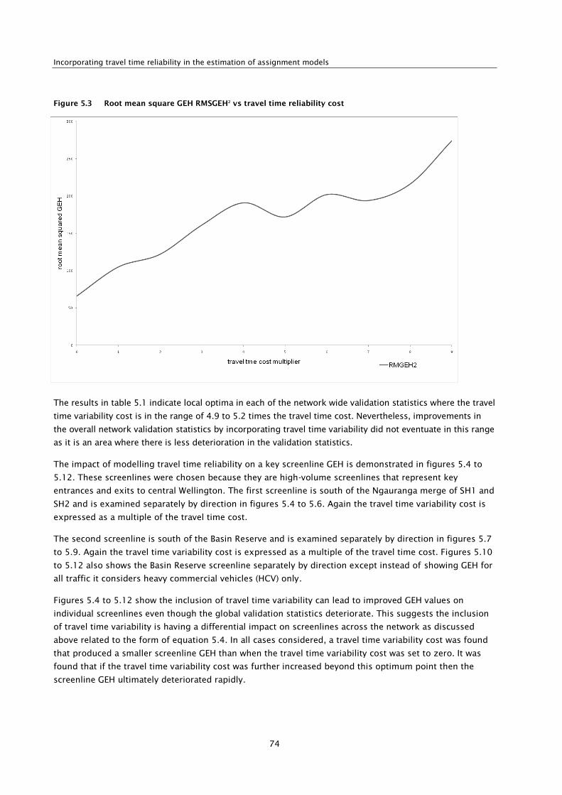
Incorporating travel time reliability in the estimation of assignment models
74
Figure 5.3 Root mean square GEH RMSGEH2
vs travel time reliability cost
The results in table 5.1 indicate local optima in each of the network wide validation statistics where the travel
time variability cost is in the range of 4.9 to 5.2 times the travel time cost. Nevertheless, improvements in
the overall network validation statistics by incorporating travel time variability did not eventuate in this range
as it is an area where there is less deterioration in the validation statistics.
The impact of modelling travel time reliability on a key screenline GEH is demonstrated in figures 5.4 to
5.12. These screenlines were chosen because they are high-volume screenlines that represent key
entrances and exits to central Wellington. The first screenline is south of the Ngauranga merge of SH1 and
SH2 and is examined separately by direction in figures 5.4 to 5.6. Again the travel time variability cost is
expressed as a multiple of the travel time cost.
The second screenline is south of the Basin Reserve and is examined separately by direction in figures 5.7
to 5.9. Again the travel time variability cost is expressed as a multiple of the travel time cost. Figures 5.10
to 5.12 also shows the Basin Reserve screenline separately by direction except instead of showing GEH for
all traffic it considers heavy commercial vehicles (HCV) only.
Figures 5.4 to 5.12 show the inclusion of travel time variability can lead to improved GEH values on
individual screenlines even though the global validation statistics deteriorate. This suggests the inclusion
of travel time variability is having a differential impact on screenlines across the network as discussed
above related to the form of equation 5.4. In all cases considered, a travel time variability cost was found
that produced a smaller screenline GEH than when the travel time variability cost was set to zero. It was
found that if the travel time variability cost was further increased beyond this optimum point then the
screenline GEH ultimately deteriorated rapidly.

5 Application to a real network
75
Figure 5.4 Observed vs modelled traffic volumes at Ngauranga inbound
Figures 5.4 to 5.6 show the impact on the Ngauranga screenline. Figures 5.4 and 5.5 show the observed
traffic volume and the modelled volume versus travel time variability cost by direction and figure 5.6
shows the respective GEH value versus travel time variability cost. It is noted that the form of the GEH
value, shown in equation 5.15
GEH = (Vobs – Vmod)2
/2(Vobs + Vmod) (Equation 5.15)
means the GEH only ever touches the horizontal axis and never crosses the horizontal axis. Nevertheless,
at the points where the GEH touches the horizontal axis the observed traffic volume equals the modelled
traffic volume or Vobs – Vmod = 0. Numerically, a sharper estimate of the travel time variability cost where
GEH is zero is obtained by examining where Vobs – Vmod = 0 rather than when GEH is zero but the zero
points are the same.
Table 5.2 summarises these results from figures 5.4 to 5.6. Estimates of the locations of the points where
GEH is zero can be found by fitting a quadratic of the form of equation 5.12.

Incorporating travel time reliability in the estimation of assignment models
76
Figure 5.5 Observed vs modelled traffic volumes at Ngauranga outbound
Using this approach it is possible to select a travel time variability cost where the GEH value is reduced to
zero for each of the inbound and outbound directions separately. Alternatively, there are locations where
the GEH value is significantly improved in both directions simultaneously but not reduced to zero. Such
locations occur when travel time variability costs are in the range 2.1 to 2.6, 3.5 to 3.8, 4.5 to 6.5 and 7.1
to 7.2.
Of particular interest is the range of travel time variability cost of 4.9 to 5.2. From table 5.1 the network
wide validation statistics are local optima. This means although the network wide validation statistics have
deteriorated when compared with the case where travel time variability cost is zero, the network wide
validation statistics have not deteriorated as much as at nearby travel time variability costs. This means
the travel time variability cost range of 4.9 to 5.2 is an area where an improved Ngauranga screenline GEH
can be found with a lesser deterioration in network wide validation statistics.
Table 5.2 Optimum GEH travel time variability costs at Ngauranga
Ngauranga
inbound
Ngauranga
outbound
Observed traffic volume 7427 4383
Traffic volume with zero travel time variability cost 8015 4631
GEH with zero travel time variability cost 6.7 3.7
Travel time variability cost multiplier where GEH = 0 2.50
3.71
4.84
6.12
7.16
2.25
3.80
7.15

5 Application to a real network
77
Figure 5.6 Ngauranga screenline GEH vs travel time reliability cost
Figures 5.7 to 5.9 show the impact of travel time variability cost on the Basin Reserve screenline. Table 5.3
summarises these results from figures 5.7 to 5.9. Estimates of the locations of the points where GEH is
zero can be found by fitting a quadratic of the form of equation 5.12.
Figure 5.7 Observed vs modelled traffic volumes at Basin Reserve inbound

Incorporating travel time reliability in the estimation of assignment models
78
Using this approach it is possible to select a travel time variability cost where the GEH value is reduced to
zero for each of the inbound and outbound directions separately. Alternatively, there are locations where
the GEH value is significantly improved in both directions simultaneously but not reduced to zero. Such a
location is a travel time variability cost in the range 3.5 to 3.9. However, this location does not coincide
with an area of local improvement in the network wide validation statistics. In the case of the Basin
Reserve screenline improving the GEH value by selecting an appropriate value in travel time reliability cost
will result in a significant deterioration in network wide validation statistics.
Figure 5.8 Observed vs modelled traffic volumes at Basin Reserve outbound
Table 5.3 Optimum GEH travel time variability costs at the Basin Reserve
Basin inbound Basin outbound
Observed traffic volume 4146 3514
Traffic volume with zero travel time variability cost (veh/hr) 4435 3338
GEH with zero travel time variability cost 4.4 3.0
Travel time variability cost multiplier where GEH = 0
3.56
4.85
6.07
3.98
4.02

5 Application to a real network
79
Figure 5.9 Basin Reserve screenline GEH vs travel time reliability cost
Figures 5.10 to 5.12 show the impact of travel time reliability cost on the Basin Reserve screenline again,
but this time for heavy commercial vehicles only. It can be seen from figures 5.10 to 5.12 there are no
values of travel time reliability cost where the GEH value becomes zero for either the inbound or outbound
direction. This is because the modelled traffic volume curve, in each direction, never intersects the
observed traffic volume.
However, even though the GEH values never reach zero there are ranges of travel time variability cost
where the GEH is improved to be better than the GEH value when the travel time variability cost is zero.

Incorporating travel time reliability in the estimation of assignment models
80
Figure 5.10 Observed vs modelled traffic volumes at Basin Reserve HCV only inbound
The points that correspond to the best GEH values correspond to the local extreme values where the
derivative of the modelled traffic volume is zero. These points can be found using equations 5.12 to 5.14.
This data is summarised in table 5.4.
Table 5.4 Optimum GEH travel time variability costs at Basin Reserve HCVs only
Basin inbound Basin outbound
Observed traffic volume 245 409
Traffic volume with zero travel time variability cost 296 350
GEH with zero travel time variability cost 3.1 3.0
Travel time variability cost multiplier for optimum GEH
4.42
7.00
3.92
GEH at optimum travel time variability cost multiplier 1.6
0.4
1.2

5 Application to a real network
81
Figure 5.11 Observed vs modelled traffic volumes at Basin Reserve HCV only outbound
Again it is possible to choose a travel time variability cost that improves the GEH value for the screenline
by direction separately. However, there is a range in travel time variability cost, being 3.7 to 4.2, where
the GEH in both directions is improved simultaneously compared with a travel time variability cost of zero.
Examination of figures 5.4 to 5.12 and tables 5.2 to 5.4 shows there is a range of travel time variability
cost where the GEH for both the Ngauranga and Basin Reserve screenlines and the Basin Reserve
screenline for HCVs only are all improved in both directions simultaneously. This range is a travel
variability cost of 3.7 to 3.8. However, at this location the global validation statistics have deteriorated
significantly. This result suggests the improvement of the GEH values at these locations comes at the
expense of the GEH values at other locations on the network.
The values of the travel time variability cost that improved GEH on the screenlines are broadly consistent
with the findings of Margiotta (2006) that the travel time variability cost was two to six times the travel
time cost.
It would be useful to examine models of other time periods in Wellington and of other cities to see if
similar results are found. This could be the subject of further research.

Incorporating travel time reliability in the estimation of assignment models
82
Figure 5.12 Basin Reserve screenline HCV only GEH vs travel time reliability cost
5.7 Impact of travel time variability on route travel time
Three routes were selected to investigate the impact of travel time variability on route travel time. Six
examples in each direction were examined by the traffic model for the morning peak period in Wellington.
The routes were as follows.
Calabar Road to Newlands ramps using SH1
Cobham Drive to Chaffers Street via Evans Bay and Oriental Parades
Cable Street by Oriental Parade to Newlands ramps on SH1 via Jervois and Aotea Quays.

5 Application to a real network
83
Figure 5.13 Travel time vs distance for various travel time reliability costs – Calabar to Newlands northbound
Travel times versus route distance for various travel time variability costs expressed as multiples of travel
time cost are shown in figures 5.13 to 5.18. Figures 5.13 and 5.14 show the Calabar Road to Newlands
ramps route using SH1 route in the northbound and southbound directions. Figures 5.15 and 5.16 show
the Cobham Drive to Chaffers Street via Evans Bay and Oriental Parades route in the northbound and
southbound directions. Figures 5.17 and 5.18 show the Cable Street by Oriental Parade to Newlands
ramps on SH1 via Jervois and Aotea Quays route in the southbound and northbound directions.
Figures 5.13 to 5.18 only show the variation in route travel time for the travel time cost multipliers of 0, 2,
4, 6 and 8 even though the analysis has been undertaken for multipliers of 0, 1, 2, 3, 4, 5, 6, 7, 8 and 9.
This has been done to improve the clarity of figures 5.13 to 5.18.
Examination of figures 5.13 to 5.18 show significant variation in travel times versus route distance except
for figures 5.16 and 5.18. Figures 5.16 and 5.18 show little variation in travel time versus route distance
for various travel time multipliers.

Incorporating travel time reliability in the estimation of assignment models
84
Figure 5.14 Travel time vs distance for various travel time reliability costs – Calabar to Newlands southbound
Table 5.5 shows the difference between the maximum and minimum route travel time for the travel time
multipliers from 0 to 9, the mean route travel time and their ratio. These are provided as measures of
variation in route travel time as a result of including travel time variability.
Table 5.5 Variation in route travel time resulting from travel time variability
Route Travel time range
(minutes)
Mean travel time
(minutes)
Range/mean
Calabar–Newlands NB 8.5 22.3 0.382
Calabar–Newlands SB 19.9 27.5 0.725
Cobham–Chaffers NB 1.7 8.7 0.197
Cobham–Chaffers SB 0.2 8.4 0.018
Cable–Newlands SB 11.6 15.8 0.737
Cable–Newlands NB 0.6 10.6 0.056

5 Application to a real network
85
Figure 5.15 Travel time vs distance for various travel time reliability costs – Cobham to Chaffers northbound
Table 5.5 presents measures of route travel time variation in response to travel time variability cost. All
routes, with the exception of Chaffers Street to Cobham Drive southbound and Cable Street to Newlands
northbound, show significant variation in route travel time in response to travel time variability cost.
Cobham Drive to Chaffers Street southbound and Cable Street to Newlands northbound show significantly
smaller travel time range and the ratio of travel time range to mean travel time ratios compared with the
other routes. Table 5.5 is consistent with the patterns observed in figures 5.13 to 5.18.

Incorporating travel time reliability in the estimation of assignment models
86
Figure 5.16 Travel time vs distance for various travel time reliability costs – Cobham to Chaffers southbound
Table 5.6 shows traffic volumes and broad volume to capacity ratios at various locations on the Wellington
network. This is to give some measure of how congested these routes are in order to understand whether
this impacts on the spread of the time versus distance curves due to travel time variability cost.
Table 5.6 Traffic volumes and broad volume to capacity measures
AADT 2009 Lanes AADT/lanes Indicative V/C
Oriental/Evans 13,700 2 6850 0.42
Calabar 22,910 2 11,453 0.70
Cobham 34,520 4 8629 0.53
Ruahine 34,370 2 17,185 1.05
Paterson 38,960 2 19,480 1.19
SH1 (SH2–Aotea) 87,130 6 14,522 0.89
SH1 (Newlands) 71,830 6 11,972 0.73
AADT = annual average daily count
V/C = traffic volume to capacity ratio

5 Application to a real network
87
Figure 5.17 Travel time vs distance for various travel time reliability costs – Cable to Newlands northbound
A broad estimate of the volume to capacity ratios at a selection of locations on the Wellington network
good enough for relative comparisons is provided in the fifth column of table 5.6. This estimate has been
obtained by taking the annual average daily traffic (AADT) measured in 2009 and divided by the total
number of lanes on the road at that location. This is converted in a morning peak-hour volume to capacity
ratio by assuming:
the morning peak is approximately 11% of the daily traffic
each lane is equally used
lane capacity is 1800 vehicles per hour.
These indicative volume capacity ratios indicate Oriental and Evans Bay Parades and Cobham Drive are
under little pressure, whereas Calabar Road and SH1 at Newlands are under moderate pressure, and
Ruahine Street, Paterson Street and SH1 from the SH2 merge to the Aotea ramps experience congestion.
No allowance for the difference in the peak direction traffic volume compared with the counter peak
direction traffic volume during the morning peak has been made in this analysis.
From table 5.5, Cobham Drive to Chaffers Street southbound and Cable Street to Newlands northbound
show significantly smaller travel time range and the ratio of travel time range to mean travel time ratios
compared with the other routes. The Cobham Drive to Chaffers Street route is largely along Evans Bay
Parade and Oriental Parade which from table 5.6 has a low indicative volume to capacity ratio.

Incorporating travel time reliability in the estimation of assignment models
88
Figure 5.18 Travel time vs distance for various travel time reliability costs – Cable Street to Newlands
southbound
The Cable Street to Newlands northbound route uses the Wellington waterfront route and SH1 (SH2-Aotea)
and SH1 (Newlands). It should be noted that the northbound route during the morning peak is in the
counter peak direction and the nominal lane capacity of 1800 vehicles per hour is on the low side. This
means the indicative volume to capacity ratios for SH1 in table 5.6 are likely to be on the high side. Hence
it is concluded the real volume to capacity ratio is likely to be low.
The remaining routes in table 5.5 have road links that are likely to have high volume to capacity ratios
using the data in table 5.6. These routes show significant variation in route travel time as a function of
travel time variability cost.
This result is consistent with the travel time variability model outlined in equations 5.3 and 5.4. This result
suggests the modelling approach using equation 5.6 to mimic the effect of travel time variability is
behaving correctly.
5.8 Summary
A number of findings can be summarised from the analysis undertaken above. These include the following:
The formulation of the standard deviation of travel time developed in this project based on a simple
function of the travel time index, CIt, appeared to be convenient for analysing the impact of travel time
reliability in traffic assignment models.
There are a number of models where traffic assignment includes the cost of travel time variability
directly in the generalised cost function. These models offer a less cumbersome incorporation of
travel time variability as they do it directly and are calibrated explicitly with travel time variability.

5 Application to a real network
89
Models, such as those based on a SATURN software platform and others, do not include travel time
variability directly in the generalised cost function. By using an iterative approach these models are
amenable to having their generalised cost function mimic travel time variability. Examination of the
literature has not revealed any case studies where a similar approach has been attempted.
The iterative approach used to mimic travel time variability appears to be numerically stable and
converges quickly. This enables the effects of travel time variability to be modelled with a reasonable
level of convenience and without requiring undue time.
Simple numerical techniques can be used to estimate optimal travel time variability costs from a range
of travel time variability costs.
The incorporation of travel time variability into an assignment model did not improve network wide
validation statistics in the case study undertaken. However, the model used already had a high degree
of model validation. Examination of local maximisation of the R2
statistic and the minimisation of the
%RMSE and RMGEH2
statistics across the network versus travel time variability cost showed the optimal
travel time variability cost was in the range of 4.9 to 5.1 times the travel time cost.
This was broadly consistent with the findings of Margiotta (2006) which is the only example found in
the literature that provides guidance on the value of the travel time variability cost. The NZTA’s (2010)
Economic evaluation manual does not provide guidance on the value of the travel time variability cost.
This was also the experience of Vincent (2008).
The incorporation of travel time variability into an assignment model did improve the GEH values of
some selected key screenlines compared with when the travel time variability cost was zero. On some
screenlines it was possible to achieve a GEH value of zero in a particular direction which represents a
perfect match of modelled and observed traffic volume
It was possible to achieve an improvement in the GEH value simultaneously in both directions. This
was achieved on all selected screenlines and produced a non zero GEH value in each direction whose
value was an improvement on the GEH value when the travel time variability cost was zero.
A travel time variability cost in the range of 3.7 to 3.8 was found to improve the GEH values of all
three selected screenlines in both directions simultaneously. However, with those values the network
wide validation statistics were worse than those for a travel time variability cost of zero.
A travel time variability cost in the range of 4.9 to 5.2 was found to improve the GEH values for the
Ngauranga screenline for both directions simultaneously and this coincided with the local optima of
the network validation statistics. This represented a region of improved matching of traffic volumes at
the Ngauranga screenline and where the deterioration in the network wide validation statistics was
less significant. This was broadly consistent with the findings of Margiotta (2006).
The examination of route travel times in response to travel time variability cost appeared to
demonstrate the correct attributes using the modelling approach advocated in this report. This
requires routes with low volume to capacity ratios to have travel times that are not sensitive to travel
time variability cost whereas routes with higher volume to capacity ratios have travel times that are
sensitive to travel time variability cost.

Incorporating travel time reliability in the estimation of assignment models
90
6 Conclusion
This study successfully achieved most of its objectives. The overall objective of this study identified in the
introduction to this report was:
... to establish whether a convenient and robust methodology was available for the
incorporation of travel time reliability in route choice algorithms of conventional assignment
models.
In order to achieve this overall objective four tasks were undertaken. Each of these tasks had a sub-
objective designed to support the overall study objective.
The first task of the research was to survey the international literature on the subject of travel time
reliability. This task successfully enabled:
an understanding of how travel time reliability influenced driver’s route choice
documentation of international experience involving travel time reliability
determination of a convenient means to mathematically describe travel time reliability
identification of known functional relationships of travel time reliability with other variables.
A second task of this study was to analyse a New Zealand travel time survey data set. This analysis
successfully:
examined the usefulness of various mathematical descriptions of travel time reliability
tested the validity of the functional relationships found in the literature review with New Zealand data
determined a convenient formulation of travel time reliability for inclusion in assignment models.
A third task of this study was to gain insights about the effect of incorporating travel time reliability on
traffic volume assignment and basic validation statistics with a simple synthetic network. This task was
successfully completed and showed if optimal values of travel time variability cost existed, these could be
found using numerical techniques. This task also showed the different responses that could be expected
depending on the assignment routine and the shape of the trip matrix.
The final task of this study was to apply the methodology for incorporating travel time reliability to a real
conventional assignment model. This showed that:
incorporating reliability was feasible
the proposed methodology was not unduly onerous and was numerically stable
the network wide validation statistics did not improve although there were ranges of travel time
variability cost where the deterioration in the network wide validation statistics was not as great
it was possible to improve the matching of modelled and observed traffic volumes on individual or
groups of screenlines but at the cost of worsening the overall network validation
travel time reliability had a differential impact on route assignment depending on congestion levels.

6 Conclusion
91
Consequently, this study achieved its objectives except it was unable to show that the incorporation of
travel time reliability would improve network wide validation in the particular case study undertaken.
Nevertheless, the inclusion of travel time reliability in assignment models is thought to be useful as it
does provide a means and rationale for improving the matching of modelled and observed traffic volumes
on individual and groups of screenlines.

Incorporating travel time reliability in the estimation of assignment models
92
7 Recommendations
From the investigations undertaken as part of this research a number of recommendations can be made in
relation to considerations regarding travel time reliability in transport planning and applications to traffic
modelling. These recommendations include the following:
The preferred measure of travel time variability should be the standard deviation of travel time.
The standard deviation of travel time can be conveniently estimated from the coefficient of variation of
travel time, which is the ratio of the standard deviation and the mean travel time, using simple
mathematical relationships.
Where estimation of the coefficient of travel time is being considered, simple functions of the ratio of
mean travel time to free-flow travel time should be investigated.
To improve the match of modelled traffic volumes and observed traffic volumes on an individual or
group of screenlines, consider the incorporation of travel time reliability into an assignment model but
note that this can also lead to worsening of the overall network validation.
To include travel time reliability in an assignment model, the travel time variability cost should be set
at a value between two to six times the travel time cost.
It is recommended further work be undertaken in the area of travel time reliability and its incorporation
into assignment models. Several areas for further research may prove useful. These include:
extension to other time periods for the Wellington case study – in particular the evening peak model
for Wellington (without travel time variability incorporated) has assignment convergence difficulties. It
would be interesting to see if travel time variability has an impact on convergence
application to a model of a city other than Wellington
recommendations immediately above could specifically consider whether the travel time variability
cost that optimises link GEH values falls into the same range found in this research or is generally
within the range found by Margiotta (2006)
application of travel time variability to a model without a high degree of validation. A variety of tests
could be undertaken to see which stage in the validation process travel time variability should be
incorporated, ie from the beginning, pre matrix estimation or post matrix estimation
further investigation of the optimal travel time variability cost for HCVs
undertaking investigation of the independence of the variances of travel time on links in a network to
consider whether the magnitude of the sum of the correlations is small compared with the sum of the
variances which will highlight the validity or otherwise of the simplifications assumed in this study.
8 References
93
8 References
Arup (2004) Journey time variability – modelling and appraisal of journey time variability. A report for the
Department for Transport, United Kingdom.
Beca Infrastructure (2009) Tauranga eastern link – toll model specification. Report prepared for the NZ
Transport Agency.
Brownstone, D, A Ghosh, T Golob, C Kazimi and D van Amelsfort (2002) Drivers’ willingness-to-pay to
reduce travel time: evidence from the San Diego I-15 congestion pricing project. University of California.
Chen, D, E van Zwet, P Varaiya and A Skabardonis (2003) Travel time reliability as a measure of service.
TRB 82nd Annual Meeting.
Cheu, K, D Stewart and B Berry (2007) Strategies for improving travel time reliability. Center for
Transportation Infrastructure Systems research report. El Paso: University of Texas El Paso.
Goodchild, A, S Globerman and S Abrecht (2007) Service time variability at the Blaine: Washington
international border crossing and the impact on regional supply chains. Research report no.3. Border
Policy Research Institute, Western Washington University.
Hollander, Y and R Liu (2008) Calibration of a traffic microsimulation model as a tool for estimating the
level of travel time variability. Leeds: Institute of Transport Studies, Leeds University.
Hyder Consulting (2007) Forecasting travel time variability in urban areas. Deliverable D1: data analysis
and model development. Department for Transport report no.0010-GD01017-TCF-02.
Hyder Consulting (2008) Forecasting travel time variability in urban areas. Deliverable D2: model
application. Department For Transport report no.0010-GD01017-TCF-02.
Lomax, T, D Schrank, S Turner and R Margiotta (2003) Selecting travel time reliability measures. Federal
Highway Administration.
Margiotta, R (2002) Travel time reliability: its measurement and improvement. 9th World Congress on ITS.
Margiotta, R (2006). Uses of travel time reliability. Presentation to Talking Operations Webinar.
New Zealand Transport Agency (2010) Economic evaluation manual. Vols 1 and 2.
www.nzta.govt.nz/resources/results.html?catid=401
Qiang, L (2007) Arterial road travel time study using probe vehicle data. Doctorial dissertation.
Department of Civil Engineering, Nagoya University, Japan.
Reckner, W, Y Chung, J Park, L Wang, A Chen, Z Ji, H Liu, M Horrocks, M and J Oh (2005) Considering risk-
taking behavior in travel time reliability. California PATH research report. UCB-ITS-PRR-2005-3.
Ruimin, L (2004) Examining travel time variability using AVI data. Victoria, Australia: Institute of
Transport Studies, Department of Civil Engineering, Monash University.
Sumalee, A and D Watling (2003) Travel time reliability in a network with dependent link modes and partial
driver response. Journal of the Eastern Asia Society for Transportation Studies 5: 1686–1701.

Incorporating travel time reliability in the estimation of assignment models
94
Tseng, Y (2005) A meta-analysis of travel time reliability. Amsterdam: Department of Spatial Economics,
Vrije University.
Vincent, M (2008) Measurement valuation of public transport reliability. Land Transport NZ research
report 339.

Appendix A: Travel time survey data summary
95
Appendix A: Travel time survey data summary
Link Direction Time of
day
Mean
journey time
(sec)
Journey time
standard
deviation (sec)
Maximum
journey time
(sec)
Minimum
journey time
(sec)
Waikanae – Whitford SBD AM 1854.5 53.57 1941 1805
IP 1775.8 31.31 1798 1721
PM 1877.4 51.89 1950 1823
NBD AM 1820.6 72.47 1916 1747
IP 1789.2 40.15 1855 1752
PM 2385.8 752.71 3716 1885
Whitford – Ghuznee SBD AM 1678.4 136.33 1884 1534
IP 885.8 22.87 916 859
PM 917.73 46.98 961 859
NBD AM 890.5 58.34 984 833
IP 883.9 49.41 969 842
PM 1060.4 154.39 1318 907
Ghuznee – Airport EBD AM 583.4 60.57 647 515
IP 569.7 69.53 685 513
PM 778.7 210.44 1120 600
WBD AM 686.1 240.8 1080 486
IP 588.7 46.92 656 543
PM 840.3 206.71 1168 634
Fergusson – Dowse SBD AM 1193.4 107.60 1333 1044
IP 1077.3 36.22 1109 1035
PM 1118.0 94.73 1219 992
NBD AM 1033.3 23.83 1069 1055
IP 1057.3 67.14 1156 993
PM 1115.9 92.83 1244 987
Dowse – Ghuznee SBD AM 1209.6 241.96 1456 819
IP 575.0 21.29 608 548
PM 792.3 318.19 1357 593
NBD AM 576.1 26.81 602 536
IP 553.9 20.50 577 528
PM 720.2 163.6 1004 601
Mungavin – Seaview EBD AM 1872.9 115.17 2023 1703
IP 1729.3 22.26 1759 1704
PM 2032.8 280.85 2424 1813
WBD AM 1927.4 91.08 2037 1787
IP 1745.1 32.81 1772 1707

Incorporating travel time reliability in the estimation of assignment models
96
Link Direction Time of
day
Mean
journey time
(sec)
Journey time
standard
deviation (sec)
Maximum
journey time
(sec)
Minimum
journey time
(sec)
PM 1936.3 213.21 2298 1668
City – Island Bay SBD AM 754.3 61.51 847 683
IP 819.3 101.81 993 743
PM 1033.0 134.02 1151 809
NBD AM 984.4 185.51 1279 817
IP 812.2 38.03 876 780
PM 1053.4 158.09 1296 901
Featherston – Upper
Hutt
SBD AM 1739.6 60.35 1823 1679
IP 1838.3 121.73 2043 1719
PM 1852.4 152.87 2116 1730
NBD AM 1799.8 43.26 1859 1737
IP 1674.0 97.15 1788 1551
PM 1740.7 107.12 1912 1649
City – Karori WBD AM 672.5 61.27 756 595
IP 628.1 30.31 680 600
PM 869.8 260.58 1285 643
EBD AM 805.6 325.09 1367 610
IP 650.1 27.85 680 615
PM 721.5 76.23 841 637
Woburn – city SBD AM 1483.8 87.73 1633 1415
IP 873.5 28.98 916 842
PM 1027.1 185.72 1321 847
NBD AM 926.6 80.94 1038 845
IP 811.2 43.91 879 775
PM 1280.1 142.59 1459 1123
Seaview – Petone WBD AM 359.0 42.86 410 292
IP 304.6 29.10 351 272
PM 309.9 25.07 338 281
EBD AM 350.8 30.75 385 307
IP 350.3 15.42 364 325
PM 435.1 115.07 597 344

Appendix B: Validation experiments
97
Appendix B: Validation experiments
Table B.1 Observed link flows
E1 E2 E3 E4 E5 E6 E7 E8
Matrix T1 T1 T2 T2 T1 T1 T2 T2.
Assign AN AN AN AN Logit Logit Logit Logit
1-2 2112 1727 2376 2372 2139 1719 2368 2368
1-4 873 475 1799 1803 841 481 1807 1807
2-1 2103 1760 2276 2068 2903 1770 2068 2281
2-3 2027 1177 2501 2497 2059 1519 2493 2493
2-4 2200 3448 2500 2500 2200 3100 2500 2500
3-2 1952 726 2400 2193 1943 720 2193 2406
3-4 1873 969 1925 2132 1883 1305 2132 1919
4-1 881 442 1894 2102 888 430 2102 1889
4-2 2317 3983 2501 2500 2320 4000 2500 2500
4-3 1747 467 1725 1728 1716 456 1732 1732
Key
E1, E2, experiment code
T1, T2 test matrix defined by equations 4.4 and 4.5
AN all or nothing assignment
Logit logit assignment
1-2, 1-4, road link from figure 4.1
2112, 873 observed link traffic volume

Incorporating travel time reliability in the estimation of assignment models
98
Appendix C: Quadratic fitting
Formulae are developed to fit a quadratic curve of the form
f = ax2
+ bx + c (Equation C.1)
through three points being (x1,f1), (x2,f2) and (x3,f3). This gives the set of three simultaneous equations
ax12 + bx1 + c = f1 (Equation C.2)
ax22
+ bx2 + c = f2
ax32
+ bx3 + c = f3
with three unknown quantities a, b and c which we seek to solve for. This means the system of equations
C.2 is solvable provided the determinant
| x12 x1 1 |
| x22 x2 1 | ≠ 0 (Equation C.3)
| x32 x3 1 |
In the system of equations C.2, if the second and the third equations are each separately subtracted from
the first equation and the first equation is retained we obtain
ax12
+ bx1 + c = f1 (Equation C.4)
a(x12 - x2
2) + b(x1 - x2) = f1 - f2
a(x12 - x3
2) + b(x1 - x3) = f1 - f3
Using equations C.4, if the first two equations are retained and (x1 - x2) times the third equation is
subtracted from (x1 - x3) times the second equation we obtain:
ax12 + bx1 + c = f1 (Equation C.5)
a(x12
- x22
) + b(x1 - x2) = f1 - f2
[(x1 - x3) (x12
- x22
) - (x1 - x2)(x12
- x32
)] = (x1 - x3)(f1 - f2) - (x1 - x2) (f1 - f3)
The system of equations C.5 allows us to solve for a, b and c.
a = -ω/Δ (Equation C.6)
where
ω = (x1 - x3)(f1 - f2) - (x1 - x2) (f1 - f3)
Δ = (x1 - x3) (x12
- x22
) - (x1 - x2)(x12
- x32
)
b = [f1 - f2 - a(x12 - x2
2)]/ (x1 - x2) (Equation C.7)
c = f1
- ax12 - bx1 (Equation C.8)
It is noted that equations C.6 to C.8 cannot be used if Δ is zero which is identical to equation C.3.

Appendix C: Quadratic fitting
99
To find a improved value of x where df/dx ≈ 0, a local optimum value then we can use f = ax2
+bx + c
where:
df/dx = 2ax + b (Equation C.9)
then we need to solve:
2aximp + b = 0 (Equation C.10)
or
ximp = -b/2a (Equation C.11)
This result is independent of c.

Incorporating travel time reliability in the estimation of assignment models
100
![RELIABILITY ESTIMATION FOR COMPONENTS - [email protected] Delhi](https://static.fdocuments.net/doc/165x107/620a64a6fbd9f168fe058116/reliability-estimation-for-components-emailprotected-delhi.jpg)


