INCORPORATING SUBJECTIVE CHARACTERISTICS IN PRODUCT DESIGN AND EVALUATIONS

Lan Luo* P. K. Kannan

Brian T. Ratchford

January 2006 Revised September 2006 Revised February 2007

Forthcoming, Journal of Marketing Research

* Lan Luo is an Assistant Professor in Marketing (e-mail: lluo@marshall.usc.edu) at the Marshall School of Business, University of Southern California, Los Angeles, CA 90089. P. K. Kannan is Harvey Sanders Associate Professor of Marketing (e-mail: pkannan@rhsmith.umd.edu) at the Robert H. Smith School of Business, University of Maryland, College Park, MD 20742. Brian T. Ratchford is Charles and Nancy Davidson Professor of Marketing (e-mail: btr051000@utdallas.edu) at the University of Texas at Dallas, Richardson, TX 75080. Please address correspondence to Lan Luo. - This research was supported in part by the U.S. National Science Foundation through Grant Number DMI 0200029. Such support does not constitute an endorsement by the funding agency of the opinions expressed in this article.

INCORPORATING SUBJECTIVE CHARACTERISTICS IN PRODUCT DESIGN AND EVALUATIONS

ABSTRACT

Consumers often use objective as well as subjective criteria to evaluate a product. For example, power tool users may evaluate a power tool based on not only its objective attributes such as price and switch type but also its subjective characteristics such as ease of use and the feel of the tool. Our research is distinctive in its emphasis on incorporating subjective characteristics in new product design. We propose a model in which consumer’s purchase intention can be impacted by both the objective attributes and the subjective characteristics. This model has the form of a hierarchical Bayesian structural equation model with the subjective characteristics treated as latent constructs. We also propose a Bayesian forecasting procedure in which the estimated relationships are used to improve the out-of-sample prediction. We illustrate our approach in two empirical studies. Our results indicate that, by collecting additional information about consumer’s perceptions of the subjective characteristics, our model can provide the product designer with a better understanding and a more accurate prediction of consumer’s product preference than the traditional conjoint models.

1

INCORPORATING SUBJECTIVE CHARACTERISTICS IN PRODUCT DESIGN AND EVALUATIONS

The existing literature in new product design has generally focused only on objective

attributes such as price and features. However, focusing only on these objective attributes can be

insufficient. For example, in addition to price and features, the determinant factors of a power

tool purchase may include qualitative characteristics such as whether the tool is perceived to be

powerful and comfortable to use. We refer to these qualitative perceptions as subjective

characteristics. In many purchase situations, both groups of factors contribute to the overall

attractiveness of the product.

Industrial designers and marketing researchers have long recognized that consumers’

perceptions of the subjective characteristics exert an important influence on their product

evaluations (e.g. Srinivasan, Lovejoy, and Beach 1997; Yamamoto and Lambert 1994). In the

consumer electronics market, many consumers prefer to touch and feel an electronic product

before purchasing (Wall Street Journal, Aug. 30, 2006). A case study by Design Management

Institute (Oct. 1997) also highlighted that one of the main reasons for the DeWalt Compact

Power Drill’s significant market success was that its design team focused on improving the

ergonomic comfort of the product. Introduced by Black & Decker in 1994, the product was an

instant success in the market and was soon the winner of numerous design awards.

While the subjective characteristics have been, by and large, informally considered at the

product design stage, there is currently no formal model that takes into account the impact of

subjective characteristics in new product design. One particular challenge is that consumers’

perceptions of the subjective characteristics often depend on a complex set of factors that can be

quite different for different individuals. For example, different people may have different views

2

as to what is emotionally appealing, comfortable, or easy to use. The levels of these subjective

characteristics are generally inferred by consumers, and their values on the measurement scales

can vary substantially across consumers. Dealing with this complexity requires an additional

modeling effort.

The objective of this paper, therefore, is to provide an effective way to incorporate

subjective characteristics in new product design. In particular, we develop a formal model that

helps the product designer to better understand the impact of the subjective characteristics on

consumer’s product preference and to incorporate such impact into the selection of optimal

product design. The model we propose has the form of a hierarchical Bayesian structural

equation model with the subjective characteristics treated as latent constructs that are determined

partly by objective attributes and partly by consumers’ idiosyncratic evaluations. In this model,

overall product evaluations are a function of both objective attributes and the latent subjective

characteristics. Unlike most existing research in new product design (with the exceptions of

Dahan and Srinivasan 2000 and Srinivasan et al. 1997), we present customer-ready prototypes to

the consumer and incorporate his/her ratings for the subjective product characteristics into the

estimation procedure. We also propose a Bayesian forecasting procedure in which the estimated

relationships are used to improve the out-of-sample prediction.

We apply our approach to the data collected in two empirical studies. The first study was

conducted jointly with a US manufacturer in the development project of a new power tool, where

the subjective characteristics tend to strongly influence consumer’s purchase intention (Design

Management Institute, Oct. 1997). To further explore the validity and generality of our model, a

second study in the toothbrush category was conducted. The results from both studies indicate

that our model provides the product designer with: 1) a better understanding of the causal

3

relationships between the objective attributes and the subjective characteristics; 2) insights into

how the objective attributes and the subjective characteristics jointly contribute to consumer’s

purchase decision; and 3) an improvement in out-of-sample prediction when used to forecast

consumer’s purchase likelihood and choice, as compared to using the traditional conjoint

models. Therefore, our model proves to be valuable in both providing diagnostics and improving

prediction.

The rest of this paper is organized as follows. First, we discuss our view of consumer

product evaluation. Second, we present the mathematical representation of our model. Third, we

compare our proposed model against several alternative models in two empirical applications.

We conclude by summarizing results, discussing limitations, and providing directions for future

research.

OUR PERSPECTIVE OF PRODUCT EVALUATION

Traditionally, most consumer preference elicitation models such as conjoint models view

a product as a bundle of objective attributes (i.e. price and features). The implicit assumption is

that consumer preference is solely a function of these attributes. The advantage of considering

only the objective attributes is that the values of these attributes are the same for everyone. As a

result, firms can collect consumers’ responses to a set of hypothetical product concepts

quantified by these attributes. However, several researchers have questioned this view of product

evaluation. For example, Srinivasan et al. (1997) have argued that consumer’s preference for a

product is only partially captured by the objective attributes. Tybout and Hauser (1981) have

found that a combination of the objective attributes and the subjective characteristics (called

“physical attributes” and “consumer perceptions” in their study) better explains consumer

preference, as compared to using just the objective attributes.

4

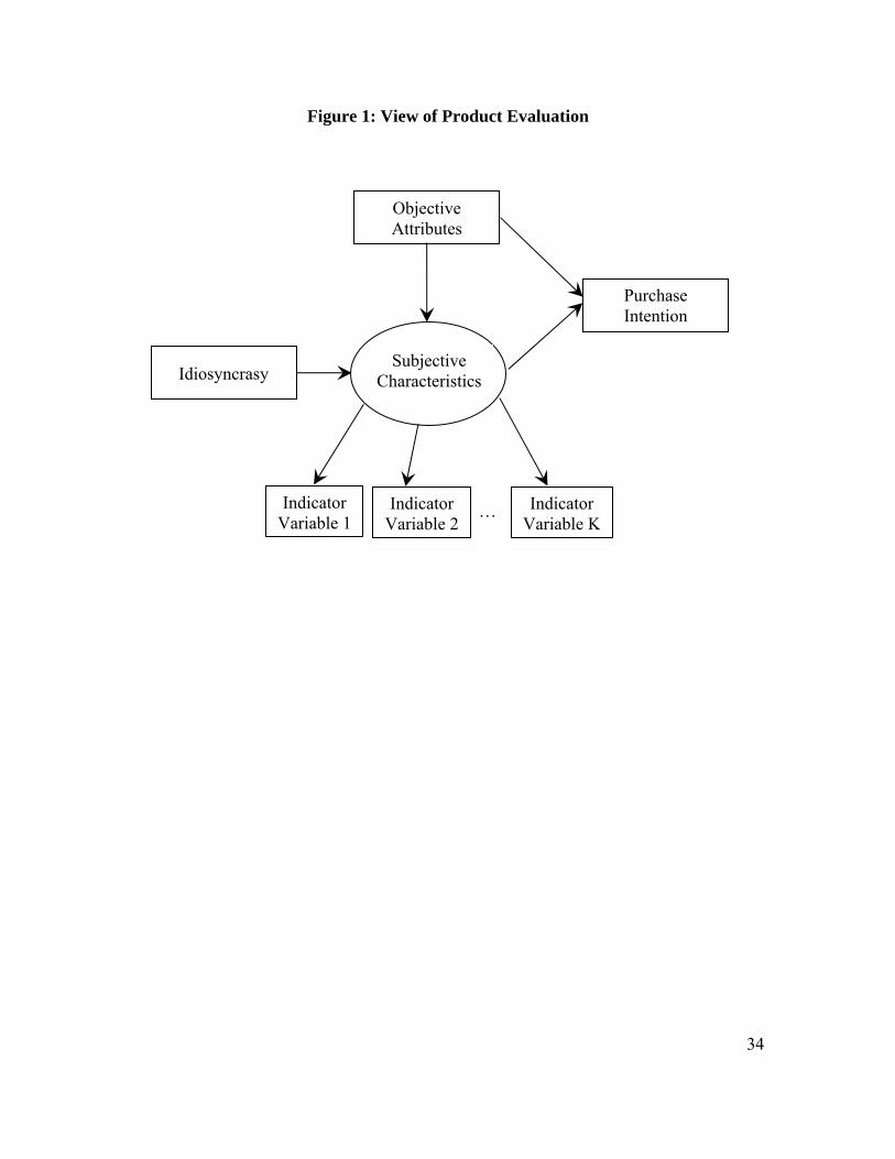
Our view of consumer product evaluation, which is outlined in Figure 1, includes both

objective and subjective criteria. Following the suggestion of Srinivasan et al. (1997), we

propose that, in order for firms to truly understand the impact of the subjective characteristics on

consumer’s purchase intention, customer-ready prototypes are necessary at the product

evaluation stage.1 In our model, each prototype is considered as a specific combination of several

objective attributes (such as shape, switch type, and weight in the power tool example), with

price included as an additional attribute. The complete set of product designs is defined by all the

possible combinations of the objective attribute levels. As the combination varies, consumer’s

perceptions of the subjective product characteristics (such as perceived power and perceived

comfort) change accordingly.

<Insert Figure 1 about here>

We view the subjective characteristics as latent constructs, with consumers’ ratings on

their perceptions of these characteristics treated as indicator variables. Modeling the subjective

characteristics as latent constructs (1) avoids the direct use of consumers’ perception ratings in

the utility function, which may provide misleading results given the presence of the

measurement errors (Ashok, Dillon, and Yuan 2002), and (2) allows for differences in precision

of ratings among individuals. For example, experts may provide more precise ratings (i.e. lower

measurement error variances) and possess more refined knowledge structure to distinguish

different latent constructs (i.e. lower factor covariances) as compared to novices (Ansari, Jedidi,

and Jagpal 2000). Accordingly, we allow the measurement error variances and the factor

covariances to vary across individuals.

1 As pointed out by Gerald M. Mulenburg (Chief of Aeronautics and Spaceflight Hardware Development Division at NASA), “it is far easier for clients to articulate what they want by playing with prototypes than by enumerating

5

Second, we define the subjective characteristics as a function of (1) the objective

attributes and (2) consumer idiosyncrasy. The former has significant support in the literature

(e.g. Griffin and Hauser 1993; Gupta and Lord 1995; Hauser and Clausing 1988; Narasimhan

and Sen 1992; Neslin 1981; Tybout and Hauser 1981). The latter, consumer idiosyncrasy,

captures additional variation in consumers’ subjective perceptions. Using power tool as an

example, while consumer with a smaller hand size may have relative preferences among

different switch types, he/she may rate the entire design space towards the low end on the scale

of perceived comfort.

Finally, we hypothesize that a consumer’s purchase intention can be impacted by both the

objective attributes and the subjective characteristics. Since the objective attributes affect

consumer’s perceptions of the subjective characteristics, a simple model with both the objective

attributes and the subjective characteristics as explanatory variables of consumer preference is

subject to the problem of multi-collinearity (Tybout and Hauser 1981). To address this issue, all

the causal relationships in Figure 1 are examined simultaneously using a hierarchical Bayesian

structural equation model (Bollen 1989). The above hypothesis derives its support from Huber

and McCann’s (1982) study which found that consumers spontaneously use the visible attributes

as cues to make inferences about the unobservable product attributes or characteristics. The

imputed values are then integrated with the available attribute information to form preferences.

Rather than imputing the unobservable values, we show that consumer perceptions of the

subjective characteristics can be measured and incorporated into a model of product evaluation.

The general framework in Figure 1 subsumes a variety of models as special cases. For

requirements” (Vision, cover story, October 2004).

6

example, the traditional conjoint model is obtained when the subjective characteristics have zero

impact on purchase intention. Alternatively, we can have a model in which the subjective

characteristics completely mediate the influence of the objective attributes on purchase intention

(i.e. the direct link from objective attributes to purchase intention in Figure 1 disappears). Or,

consumers’ perceptions of the subjective characteristics can be driven by a subset of the

objective attributes in the design space. Furthermore, different consumers can make inferences

on the subjective characteristics from different subsets of the objective attributes. The relative

importance of consumer heterogeneity in evaluating these attributes may also vary across

product categories.

The merit of our proposed model lies not only in its flexibility to accommodate the

various possibilities but also in its ability to provide the product designer with valuable answers

to these empirical questions. For example, the empirical results from our model may suggest that

the subjective characteristics do not play an important role in a laptop purchase. This may imply

that the marketers should promote the objective attributes (e.g. a high resolution monitor, a long

battery life) when launching new laptops. Alternatively, researchers using our model may find

that the purchase of sunglasses is purely driven by consumer’s perceptions of the subjective

characteristics such as perceived comfort and aesthetics. That is, the impact of the objective

attributes on purchase intention is completely mediated by these subjective characteristics.

Under such a scenario, marketers may need to communicate the aesthetics and comfort of the

sunglasses to the consumers. Even when both the objective attributes and the subjective

characteristics affect consumers’ purchase decisions (probably the case for most purchases), it is

useful to understand the underlying causal relationships. For example, without accounting for the

subjective characteristics, a traditional conjoint analysis may suggest that consumers are more

7

likely to purchase an office chair when it is offered at a high price. However, our model may

suggest that consumers perceive a high priced office chair to be more durable, which leads to a

higher purchase intention, and that the direct impact of price on purchase intention is actually

negative. If the marketers ignore the role of the subjective characteristics, they may position their

products as “luxurious” office chairs rather than “durable” office chairs.

Finally, it is likely that the most important application of this model is for predictive

purposes in estimating potential demand for new design concepts. Given the design space

defined by all the possible combinations of the objective attribute levels, we posit that firms only

need to develop a subset of the product concepts into prototypes. Using the estimated

relationships between the objective attributes and the subjective characteristics, we can forecast

the values of the subjective characteristics for the out-of-sample product alternatives. Such

predictions, along with the other estimated relationships in the model, can be used to forecast the

purchase likelihood of these alternatives and thus determine the optimal design.

Ashok et al. (2002) also considered a model that incorporated latent attitudes and

perceptions. However our approach is different in focus and execution. While Ashok et al.

(2002) made an important contribution by demonstrating how to incorporate latent attitudes into

discrete choice models, their focus was mainly on perceptions of satisfaction and other latent

attitudes of existing products. Since these attitudes might exist independently of the objective

product attributes, Ashok et al. (2002) did not explore relationships between objective attributes

and latent attitudes. In contrast, our primary focus is on product design and on the relationship

between objective attributes and subjective characteristics. Thus, we model subjective

characteristics as a function of objective attributes and individual-specific effects, and purchase

intent as a function of both objective attributes and subjective characteristics.

8

MODEL DEVELOPMENT

The Hierarchical Bayesian Structural Equation Model

We use a hierarchical Bayesian structural equation system to form the basis of our model.

We specify the relationships outlined in Figure 1 for each individual. At the population level,

population distributions are specified to model variations in individual-level parameters.

Let i =1 to N represent the individuals and let s =1 to S index the product profiles used in

the calibration sample. Suppose that these product profiles are constructed in a fractional

factorial design using the orthogonal design criterion (Addelman 1962) and are developed into

prototypes. Each individual provides the following information: 1) purchase likelihood of each

prototype (denoted as ispr ) and 2) answers to a series of questions that assess his/her perceptions

of the subjective product characteristic (denoted as a ( 1×K ) vector isv ). Let sx denote the

( 1×M ) vector of objective attributes. Let isz be the ( 1×J ) vector of latent constructs

representing individual i’s perceptions of the subjective characteristics of prototype s, with the

( 1×K ) vector isv being the observed indicator variables.

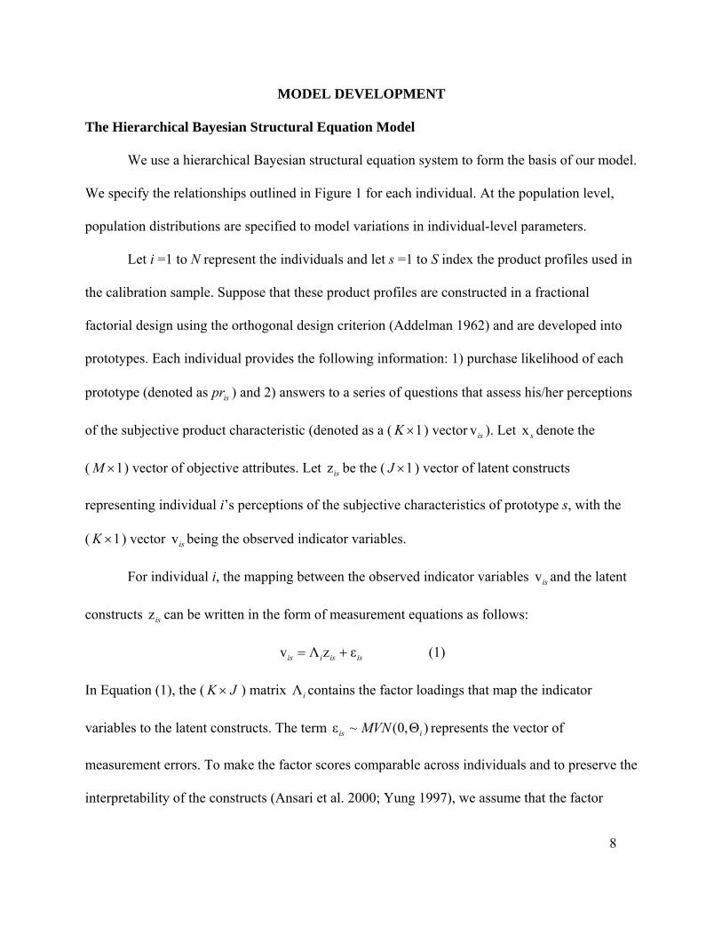
For individual i, the mapping between the observed indicator variables isv and the latent

constructs isz can be written in the form of measurement equations as follows:

isisiis εzΛv += (1)

In Equation (1), the ( JK × ) matrix iΛ contains the factor loadings that map the indicator

variables to the latent constructs. The term )Θ,0(~ε iis MVN represents the vector of

measurement errors. To make the factor scores comparable across individuals and to preserve the

interpretability of the constructs (Ansari et al. 2000; Yung 1997), we assume that the factor

9

loading matrices are invariant across individuals, i.e., ΛΛ =i , for Ni ,..,1= . Following the

tradition in confirmatory factor models, we also set the appropriate elements in the loading

matrix Λ to be unity for identification.2 Finally, the ( KK × ) matrix, iΘ , is diagonal with the

measurement error variances varying across individuals. Specifically, we assume that each

measurement error variance comes from an independent inverse gamma population distribution.

The structural equation relating consumer idiosyncrasy and the objective attributes to the

subjective characteristics for each individual is:

issiis μxBδz i ++= (2)

In Equation (2), iδ represent the ( 1×J ) vector of idiosyncratic terms, iB is a ( MJ × ) coefficient

matrix denoting the effects of sx on isz , and the ( 1×J ) vector of )Δ,0(~μ iis MVN represents the

disturbance terms. We fix 1δ to be zero for identification. This is similar to fixing the intercept

of one group to zero in a multi-group analysis (Sörbom 1981). We also assume that the jth row

vector (denoted as ijb ) in the coefficient matrix )''b,...,'b,'b(B 21 iJiii = is distributed multivariate

normal from a population distribution. Finally, we allow the ( JJ × ) variance-covariance matrix

iΔ to vary across individuals with an inverse Wishart population distribution.

Now let us consider the structural equation of purchase intention. For individual i , the

indicated purchase likelihood for product profile s is ispr . Following the common practice in

conjoint studies (Mahajan, Green, and Goldberg 1982; Moore, Gary-Lee, and Louviere 1998;

2 While this structural approach explicitly accounts for measurement errors in isv , we acknowledge that our model could possibly become over-parameterized. An alternative approach would be to use the average ratings of isv to represent the subjective characteristics, which would result in a hierarchical Bayesian path analysis model. We present a summary comparison between these two different modeling approaches in our empirical application section; details of this comparison are contained in an Appendix that is available at the publisher’s website.

10

Sawtooth CVA User’s Manual 2002), we employ a logit transformation on ispr to ensure that the

predicted purchase likelihood for each profile in the design space is bounded between 0 and 1.

Therefore, we have the following:

isisisiisis

is eypr

pr++==⎟⎟

⎠

⎞⎜⎜⎝

⎛−

zγxA1

ln (3)

In Equation (3), iA is a ( M×1 ) vector reflecting the direct impact of the objective attributes on

purchase intention, iγ is a ( J×1 ) vector denoting the influence of the subjective characteristics

on purchase intention, and ),0(~ 2eis Ne σ denotes the error term. Specially, we assume that the

row vector of γ,Aη iii = is distributed from a multivariate normal population distribution.

In summary, after taking into account the individual-level model and the heterogeneity

specifications, the complete hierarchical Bayesian model can be written as follows:

Individual- Level Model

),0(~

)Δ,0(~μ)Θ,0(~ε

zγxAμxBδz

εΛzv

2eis

iis

iis

isisisiis

issiiis

isisis

Ne

MVNMVN

ey

σ

++=++=

+=

(4)

Population-Level Model

)Ω,φ(~η

)D,β(~b)Σ,κ(~δ

)R,ρ(~Δ

),(~)Θ(1

MVN

MVNMVN

W

IGdiag

i

jjij

i

i

kkiik−

= ψςθ

(5)

Given our model setup, an alternative model would be a traditional conjoint model using

for Kk ,...,1=

for Jj ,...,1=

11

prototypes as stimulus presentation, e.g., a model directly relating isy to sx . The key difference

between our model and a traditional conjoint model is that we collect consumer’s ratings on the

subjective characteristics as augmented data. As long as these subjective perceptions ( isz )

contain information about the individual (i) that is independent of the objective attributes ( sx ), it

is possible for our model to better explain purchase intent ( isy ) than the traditional conjoint

model. The separate individual-level intercepts (δi) allow this relation between subjective

perceptions and personal characteristics to be captured. However, even if δi were the same across

individuals, Bi and γi in Equation (4) could vary across individuals. In order to replicate the

results implied by our model from estimating the relationship between isy and sx , one would

need to capture the resulting distribution of the product of Bi and γi. Therefore, because our

model incorporates additional information on subjective characteristics ( isz ) that can influence

purchase intent ( isy ), we expect the proposed model to have incremental in-sample fit over the

traditional conjoint model.3

The estimation of this model is carried out in a Markov Chain Monte Carlo (MCMC)

procedure. In particular, the unknown parameters in our model are given

by Ω,φ,D,β,Σ,κ,R,ρ,,,,Λ 2jjkke ψςσ . The joint density of all model parameters can be

expressed as follows:

3 The proposed model can be identified as long as isz and sx are not perfectly correlated. When there is independent

variation in isz not explained by sx , and this helps to explain isy , the proposed model remains valid. And this

identification becomes more precise as the independent variation in isz increases. If isz were perfectly collinear

with sx , Equation (4) would not be identified. However, a reduced-form relation between isy and sx (the traditional conjoint model) could still be estimated.

12

)Ω,φ,D,β,Σ,κ,R,ρ,,,,Λ(

)R,ρΔ(),()Δμ()D,βb()Σ,κδ()ε(

)()Ωφη()μ,b,δ,xz()ε,Λ,zv(),η,z,x(

)v,Ω,φ,Δ,β,Σ,κ,R,ρ,,,,Λ(

2

2

11

2

jjkke

ikkikiisjjijiikis

eisiisijisisisisisisiissis

S

s

N

i

isisjjkke

f

ffffff

effffeyf

yf

ψςσ

ψςθθ

σ

ψςσ

,==ΠΠ∝

(6)

Gibbs Sampler and the Metropolis-Hastings algorithm are used to sample draws from the

full conditional distribution of each block of the parameters.4 The outputs of our Bayesian

estimation are the posterior distributions of these parameters, with all the underlying

relationships in the model accounted for simultaneously.

Prediction Procedure for Out-of-Sample Product Alternatives

In this section, we discuss how to use these posterior distributions to predict the values of

the subjective characteristics and purchase likelihood for product concepts not included in the

calibration sample. Our main premise is that, for these out-of-sample product alternatives, the

latent measures of the subjective characteristics can be predicted from the estimated links

between the objective attributes and the subjective characteristics. And such predictions, along

with the other estimated relationships in the model, can be used to predict the purchase

likelihood of these products.

We first describe the procedure of estimating the posterior predictive distribution of the

latent factor scores. In our calibration sample, the posterior distribution of the factor scores isz is

estimated based on the priors and information from two data sources. The first data source is the

measurement equation isisis εΛzv += . The second data source is from the structural

equation issiiis μxBδz ++= . Therefore, the full conditional distribution of isz can be written

4 The prior distributions, the conditional distribution for each block of the model parameters, and the simulation steps involved in the MCMC procedure are provided in an Appendix available at the publisher’s website.

13

as )Δ,ω(iis zzMVN , where ]vΘ'Λ)xBδ(Δ[Δω 11

isisiiizz iis

−− ++= and ΛΘ'ΛΔΔ 111 −− += ii-

iz. Let g

=1 to G represent the index of the out-of-sample product alternatives, gx denote the vector of the

objective attribute combination for product g , and pigz be the vector of predicted factor scores.

The posterior predictive distribution of pigz can be expressed as )Δ,ω(

iig zzMVN with

]vΘΛ')xB(δ[ΔΔω 11isigiiizz iig

−− ++= andizΔ as defined above. The basic idea is that, when the

combination of the objective attribute levels changes from sx (in-sample) to gx (out-of-sample),

we can use the posterior distribution of the model parameters to forecast the individual-level

subjective perceptions (i.e. pigz ) for the out-of-sample product alternatives.

Now we explain the procedure of estimating the posterior predictive distribution of

purchase likelihood. Let Ω,φ,D,β,Σ,κ,R,ρ,,,,Λ 2jjkkeξ ψςσ= denote all the

parameters in our model, pigy be the predicted purchase intention of individual i for product

alternative g , and pgPr be the expected purchase likelihood of product g over the entire sample

of subjects. Given a particular objective attribute combination (i.e. gx ), the posterior predictive

distribution of purchase likelihood (i.e. pgPr ) can be calculated from random draws of the

parameters from the posterior distribution (Equation 7):

dξyξfξfξyfy

yyf isisg

pig

pigg

pigp

ig

pig

N

iisisg

pg )v,(),xz(),z,x(

)]exp(1[)exp(

)v,,x(Pr 21 +

= ∫Π=

(7)

In Equation (7), the first component in the integral is the conditional predictive density

distribution of the purchase likelihood, the second component is the conditional predictive

distribution of purchase intention, the third component is the conditional predictive distribution

14

of the individual-level factor scores (discussed earlier), and the last component is the posterior

distribution of model parametersξ . As discussed by Rossi and Allenby (2003), one advantage of

this full Bayesian prediction approach is that the uncertainties in the model parameters are

factored into the managerial decision itself.

Given the procedure summarized in Equation (7), the product designer can predict the

purchase likelihood of the out-of-sample product alternatives given their objective attribute

values and the estimated relationships in the model. Because the values of the subjective

characteristics are predicted from the objective attributes and these predictions are used to limit

the error in the prediction of purchase likelihood, we expect our model to do better in out-of-

sample prediction than the traditional conjoint model. An optimal design from the entire design

space can then be selected based on the posterior means of the predicted purchase likelihood.

EMPIRICAL APPLICATIONS

In this section, we illustrate the proposed model in two empirical applications. We also

compare the in-sample fit and predictive power of this model to several benchmark models.

Study One: The Design of a Handheld Power Tool

Data

The study context was the design of a handheld power tool by a US manufacturer. Based

on exploratory research and field studies, we identified four objective attributes (shape, switch

type, weight, and price) and two subjective characteristics (perceived power and perceived

comfort) as the important objective and subjective criteria for the users of this power tool.5

Brand was not included as an objective attribute because its impact on purchase intention is

5 Some supplemental information related to both empirical studies (e.g. experimental design, stimulus description, auxiliary estimation results) are provided in an Appendix available at the publisher’s website.

15

identical across all the design candidates. Given the various combinations of the objective

attribute levels, 10 product profiles were constructed in a fractional factorial design using

orthogonal design criterion (Addelman 1962). These product profiles were developed into

customer-ready prototypes.

The data for this study were collected from 51 construction and metal workers recruited

from various job and construction sites in a large metropolitan area. Ten customer-ready

prototypes were presented for evaluation. Each prototype was painted grey and had an attached

price tag. Our experiment consisted of two stages.

In stage one, we asked the participants to imagine that they were shopping for the power

tool in a retail store. The participants had an opportunity to touch and feel each prototype before

providing their purchase likelihood ratings on an 11-point scale anchored at “extremely

unlikely” and “extremely likely”. We purposely did not ask the participants about their opinions

on any of the subjective characteristics at this stage because previous research has indicated that

the prompting of inferences may significantly alter consumer’s preference (Huber and McCann

1982).

At the second stage, additional information was collected on the participants’ subjective

perceptions. We used a 3-item measurement on a 7-point scale ranging from “strongly disagree”

to “strongly agree” to measure perceived power (i.e. “I expect this tool to be powerful”; “This

tool feels weak” (reverse coding); “This tool may not be powerful enough to do my job” (reverse

coding)). A 4-item measurement scale was used to measure perceived comfort (i.e. “The grip of

this tool feels comfortable”; “This tool feels balanced”; “This tool is difficult to use” (reverse

coding); and “The configuration of this tool will allow me to do my job without any kind of

obstruction”). A pretest with 80 observations across 8 participants was conducted to assess the

16

validity and reliability of these measurement scales. The convergent and discriminant validities

were tested through confirmatory factor analysis (Bollen 1989) and the Cronbach’s alpha for

perceived power was .778 and for perceived comfort was .747. Standardized values of the

subjective measures were used in our analysis.

Models

We used data from the first nine prototypes for calibration. We estimated the following

models on the calibration sample. Model 1 is the proposed model. In Model 2, only the latent

constructs of the subjective characteristics are used as explanatory variables of purchase

likelihood.6 In Model 3, purchase likelihood is solely a function of the objective attribute

values.7 We kept the hierarchical Bayesian method as the common denominator for all three

models so that the comparisons of model-fits could be purely ascribed to the underlying

relationships in the models and not to improvement from the use of a Bayesian technique. In

particular, Model 3 is identical to a prototype-based conjoint model estimated by a hierarchical

Bayesian (HB) technique. 8

Measures of In-Sample Fit

We use the following three measures to assess the in-sample fits of these models:

1. The percentage of variance accounted for:

6 Mathematically, the individual-level model can be expressed as: isisiiisisisis ey ++=+= zγ;εΛzv α . The heterogeneity specifications and the population-level distributions are similar to the specifications in the proposed model. The mathematical representation of this model is kept similar to that of the proposed model so that the difference in model-fits can be ascribed purely to the exclusion of the objective attributes. 7 The individual-level model can be presented as: issiiisy ϖβ ++= xπ . The heterogeneity specifications and the population-level distributions are similar to the specifications in the proposed model. 8 We also conducted an ordinary least square (OLS) conjoint estimation at the individual level. Because the number of observations per subject equals the number of parameters, our individual OLS estimation did not provide satisfactory results. Therefore, we did not report the individual OLS estimation results in the paper.

17

Pseudo∑∑

∑∑

= =

= =

−

−= N

i

N

sis

N

i

N

sis

yy

yyR

1 1

2

1 1

2

2

)(

)ˆ( (8)

where isy is the predicted purchase likelihood and y is the average of all observations.

2. Deviance Information Criterion (DIC) (Spiegelhalter, Best, Carlin, van der Linde

2002):

DpDDIC 2)( += ξ (9)

where ))y(log(2)( ξξ fD −= is the deviance obtained by substituting the posterior means of the

model parameters into the log-likelihood function of the observed y isy= ;

and ))y(log(2)]y(log(2[ ξξξ ffEp yD +−= represents the effective number of model parameters.

A smaller DIC value indicates a better model-data fit after the complexity of the model is

penalized.

3. Posterior predictive check of internal validity (Gelman, Meng, and Stern 1996; Jedidi,

Jagpal, and Machanda 2003): First, we generate a replicated data set of repisy using the observed

values of the explanatory variables and the posterior distribution of the model parameters

(denoted asξ ). The posterior predictive distribution of repisy can be expressed as:

dξyξfξyfyyf isrepisis

repis )()()( ∫= (10)

Next, we compare the replicated data set and the actual data set using a discrepancy

variable defined as:

SN

yyRMSD

is

N

i

S

s

repis

*

)( 2

1 1−

=∑∑= = (11)

18

The advantage of this internal validity check is that it considers both the mean and the

variance of the prediction and is free of asymptotic definitions.

Results of In-Sample Fit Comparisons:

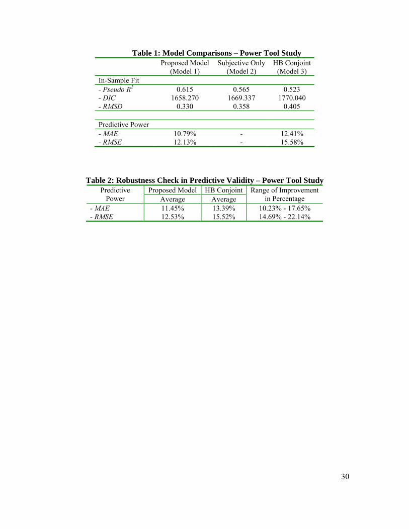
The results of the in-sample fit comparisons are presented in the top panel of Table 1.

With regard to the Pseudo R2 measure, the proposed model explained the most variance in the

observed purchase likelihood as compared to the other models. Because the key difference

between the proposed model and the subjective only model is the exclusion of objective

attributes, we observed that an additional 5% (i.e. 0.615 - 0.565) of the variance in purchase

likelihood is explained by the addition of the objective attributes. Similarly, a comparison

between the proposed model and the HB conjoint model suggests that an extra 9.2% (i.e. 0.615 –

0.523) of the variance in purchase likelihood is contributed by the subjective characteristics in

the proposed model. When both the objective attributes and the subjective characteristics

influence purchase likelihood, dropping either group of data from the explanatory variables of

purchase likelihood results in a loss of model fit. In the power tool application, the loss due to

the exclusion of the subjective characteristics is relatively larger than the loss due to the

exclusion of the objective attributes (i.e. 9.2% vs. 5%). Even with the use of DIC measure, which

penalizes the more complex model, we found that the proposed model provided the smallest DIC

value, followed by the subjective only model and the HB conjoint model. A similar pattern is

found for the discrepancy measure, RMSD.

<Insert Table 1 about here>

Measures of Predictive Power

Next, we examine the predictive power of these models. In practice, researchers often

need to predict the purchase likelihood of the out-of-sample products based on their physical

19

configurations (i.e. the values of the objective attributes). Therefore, in the holdout sample, only

the values of the objective attributes are used to predict purchase likelihood.9 The prediction

procedure for Model 1 is summarized in Equation (7). The prediction procedure for Model 3

follows the convention of conjoint models. Specifically, the following two measures are used to

assess the predictive power:

1. The mean-absolute-error (MAE) between the true ( ihPr ) and estimated ( ihrP ) purchase

likelihood in hold-out sample ( h is the index for holdout profile):

( )HN

MAE

N

i

H

hihih

*

rPPr1 1∑∑= =

−= (12)

2. The root-mean-square-error (RMSE) between the true ( ihPr ) and estimated ( ihrP )

purchase likelihood in hold-out sample ( h is the index for holdout profile):

( )HN

RMSE

N

i

H

hihih

*

rPPr2

1 1∑∑= =

−= (13)

Results of Predictive Power Comparisons:

We first compared the actual purchase likelihood data collected on prototype #10 with

the predicted purchase likelihood. As evident in the second panel of Table 1, the proposed model

was able to predict the actual purchase likelihood better than the HB conjoint model (smaller

MAE and RMSE).

Because we collected purchase likelihood data and the subjective characteristic ratings

from all 10 prototypes, we further investigated the predictive power of the proposed model and

the HB conjoint model in a robustness check. A hold-one-out validation was conducted

9 Model 2 lacks predictive power because the objective attributes are not included in the model.

20

iteratively. First, we chose one prototype among the ten prototypes as the holdout prototype.

Next, we calibrated the model on the remaining nine prototypes. Finally, we used the model

estimates to predict the purchase likelihood of the holdout prototype. We repeated this procedure

until each of the ten prototypes had been selected as the holdout prototype. In each prediction

scenario, only the values of the objective attributes were used to predict the purchase likelihood

of the holdout prototype.

Table 2 provides the average MAE and the RMSE measures of both the proposed model

and the HB conjoint model over the 10 prediction scenarios. For each prediction scenario, we

also calculated the percentage of improvement in MAE and RMSE measures when the proposed

model was compared against the HB conjoint model. For example, when prototype #10 was used

as holdout prototype (Table 1), the percentage of improvement in MAE is calculated as 13.05%

(i.e. (12.41%-10.79%)/12.41%). The ranges of the percentage improvement were shown in the

last column of Table 2.

<Insert Table 2 about here>

Overall, our model comparisons and robustness check indicated that the proposed model

outperformed the benchmark models in goodness-of-fit and out-of-sample prediction.

Parameter Estimates of Models

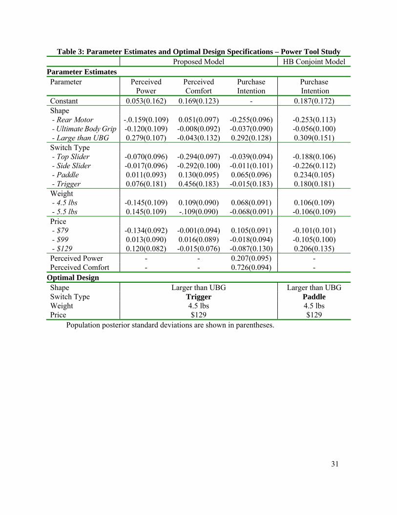
Table 3 reports the parameter estimates from the proposed model and the HB conjoint

model. The population posterior standard deviations are provided in parentheses as an indication

of heterogeneity in preferences within the population. Columns 2-4 in this table provide the

estimates from the proposed model. As we can see, there is a large dispersion in the idiosyncratic

terms of perceived power and perceived comfort. This indicates that the idiosyncratic

characteristics play an important role in determining the heterogeneous subjective perceptions

21

across individuals. With respect to perceived power, our model estimates indicate that, in

general, switch types did not have a large influence on consumer’s perceptions of whether the

tool is powerful. Among the other product attributes, a larger than UBG shape, heavy-weight,

and high priced power tool was perceived as being powerful. This is consistent with previous

research on price-quality inference (e.g. Rao and Monroe 1989 and 1996). In terms of perceived

comfort, consumers did not seem to relate price levels to comfort. In contrast to perceived

power, a light-weight power tool was considered to be comfortable to use. In addition, a trigger

switch was perceived to be the most comfortable at the population level, while the heterogeneity

across individuals was also relatively high. With regard to purchase intentions, consumers valued

perceived comfort more than perceived power when making purchase decisions. These

subjective characteristics partially mediated the influences of the objective attributes on purchase

intention. In particular, the direct effect of higher prices on purchase intention was negative. The

last column of Table 3 gives the model estimates from the HB conjoint model. This model

suggests that consumers preferred a high priced power tool. According to what we observed in

the proposed model, the consumers preferred such a power tool because they perceived it to be

powerful, not because they liked to pay more.

<Insert Table 3 about here>

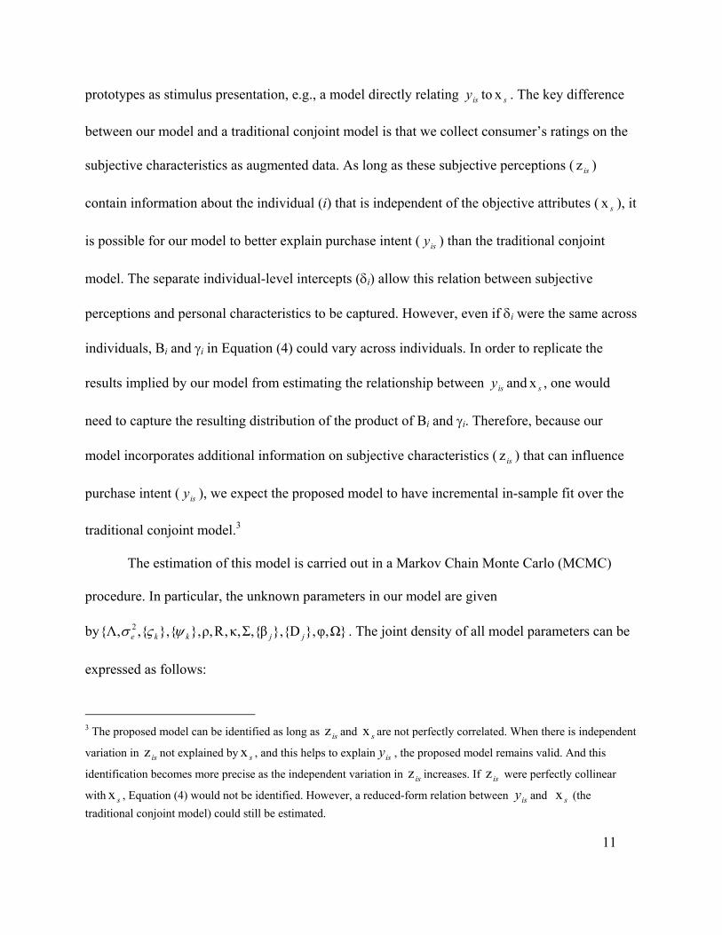
Given our model estimates, the total effects of changing an objective attribute (direct

effect on purchase intention plus indirect effect on subjective perceptions) can be calculated. Let

us consider the effects of paddle and trigger switches in Table 3. At the population level, the

total effect of paddle on purchase intention could be obtained as:

Paddle effect = 0.065 + 0.207*0.011 + 0.726*0.130 = 0.162,

where 0.065 is direct effect, 0.207*0.011 is power effect times effect of paddle on power, and

22

0.726*0.130 is effect of comfort times effect of paddle on comfort. A similarly calculated

average effect of trigger would be:

Trigger effect = -0.015 + 0.207*0.076 + 0.726*0.456 = 0.332.

Because it is viewed as more comfortable, and because comfort is an important

characteristic, the trigger effect is seen to be considerably larger than paddle, even though its

direct effect is negligible. In contrast, the standard conjoint model indicates that paddle is more

attractive. Incorporating perceptions of comfort into the analysis revealed that the trigger is the

better design alternative.

Finally, we used the procedure summarized in Equation 7 to predict the purchase

likelihood of the out-of-sample product alternatives. The optimal design was selected as the one

with the highest overall purchase likelihood (i.e. highest posterior mean) in the design space. A

comparison in the optimal design specifications reveals that the optimal product designs

identified by the two models differ in switch types (Table 3). Defining consumers’ purchase

intention as a function of only the objective attributes, the HB conjoint model did not provide an

as accurate prediction of purchase likelihood as the proposed model. As a result, the HB conjoint

model identified a suboptimal switch type in the optimal design selection.

We also estimated a hierarchical Bayesian (HB) path analysis model in which the average

ratings of perceived power and perceived comfort were used to represent the values of the

subjective characteristics. There is a considerable similarity in the parameter estimates from the

proposed model and the path model, except that the subjective characteristics have a relatively

smaller impact on purchase likelihood in the path model than in the proposed model. This is

consistent with the findings in Ashok et al. (2002). Our conjecture is that, because the path

model does not account for the measurement errors in the subjective characteristic ratings, the

23

impact of these subjective characteristics appeared to be smaller in the path model than the

proposed structural model. Regarding in-sample fit and out-of-sample prediction, the proposed

model demonstrated better in-sample fit (in terms of Pseudo R2 and RMSD) and out-of-sample

prediction (in terms of MAE and RMSE) than the path model.10

Study Two: The Design of a Toothbrush

Data

In practice, the majority of conjoint experiments are paper-and-pencil or web-based

studies. Therefore, in Study 2 we further investigated the relative performance of the proposed

model as compared to both verbal and prototype-based conjoint models. In addition, by

simulating a realistic retail environment, we assessed the ability of the competing models in

predicting actual choice behavior.

The data for this study were collected from undergraduate marketing students in a large

mid-Atlantic university. At the exploratory stage, we collected different designs of toothbrushes

through field visits to retail outlets. We then conducted pretests to identify the set of objective

attributes (i.e. price, softness of bristles, head size, bristle design, angle of head, and grip design)

and subjective characteristics (i.e. perceived effectiveness and perceived comfort) used in this

study. Brand was not selected for the same reason we discussed in the power tool study. Among

the toothbrushes collected in the field, 14 toothbrushes with various combinations of attribute

levels were chosen for our study.

We included two experimental conditions in this application. The experimental setup in

Condition 1 is similar to that of the power tool study. We masked the brand name and attached a

10 Details are presented in an Appendix that is available on the publisher’s website.

24

tag to each toothbrush indicating its price and the softness of the bristles.11 In Condition 2, we

conducted a verbal conjoint survey using Media Lab. Pictures of the toothbrushes were taken to

depict their bristle and grip designs. Other attributes were described verbally. The participants

were asked to provide their purchase likelihood ratings on an 11-point scale for each of the

toothbrushes. Condition 1 comprises 1176 observations across 84 participants, and Condition 2

consists of 896 observations across 64 participants.

In Condition 1, after providing the purchase likelihood ratings on a scale from 1 to 11

(stage one), the participants were asked to rate each toothbrush on whether they perceived it to

be effective or comfortable to use (stage two). We used a 4-item measurement on a 7-point scale

ranging from “strongly disagree” to “strongly agree” to measure the perceived effectiveness (i.e.

“I expect this toothbrush to work well”; “I expect this toothbrush to be very effective in cleaning

my teeth”; “This toothbrush will perform better than an average toothbrush”; and “This

toothbrush will do a good job in preventing tooth decay”). A 3-item measurement scale was used

to measure the perceived comfort (i.e. “I expect this toothbrush to be more comfortable than an

average toothbrush”; “This toothbrush is difficult to use” (reverse coding); and “The design of

this toothbrush is awkward” (reverse coding)). A pretest study with 140 observations across 10

participants was conducted to assess the validity and reliability of these measurement scales. The

convergent and discriminant validity of these scales was examined through confirmatory factor

analysis. The Cronbach’s alpha for perceived effectiveness is .937 and perceived comfort is .713.

Standardized values of the subjective measures were used in our analysis.

In both conditions, we offered each respondent $5 at the beginning of the study to

11 Our pilot study revealed that the respondents could not identify the brand names of the masked toothbrushes by just observing their attributes.

25

purchase one toothbrush from a set of five toothbrushes. The toothbrushes available for purchase

were chosen to represent five out-of-sample product alternatives in the design space (i.e. their

product specifications differ from the 14 toothbrushes used in the main study). Because this

choice experiment simulates a realistic retail environment in which consumers choose among

several competing products, it helps us to examine how well each of the competing models can

predict actual choice behavior. At the end, the chosen toothbrush and the amount remaining from

the $5 were given to each participant.

Model Comparisons

We used data from the first 12 toothbrushes for calibration. In Condition 1, we examined

the in-sample fit of three models (i.e. proposed model, subjective only model, and HB conjoint

model). In Condition 2, we estimated a HB conjoint model.12

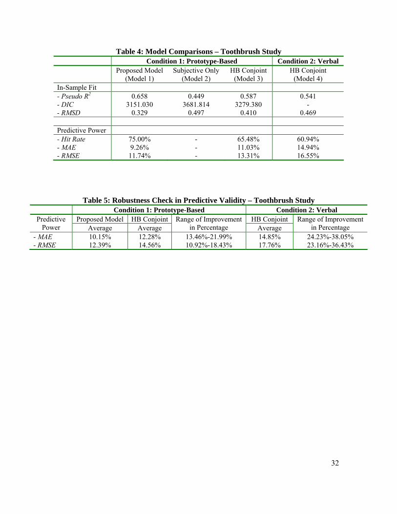
The results of the in-sample fit comparisons shown in the top panel of Table 4 indicate

that the proposed model was superior to the alternatives on all measures.13 The predictive power

of the models is reported in the second panel of Table 4. Similar to the prediction procedures

described in the power tool application, only the values of the objective attributes were used in

the out-of-sample predictions. In the Hit Rate prediction, we used the first choice rule (i.e. the

respondent chooses the product with the highest overall utility) to predict the actual choice

behavior of each participant under each model. A hit occurs when the model correctly predicts

which of the five toothbrushes was chosen by the respondent. Among the four models under

12 We also estimated a HB path analysis model for the toothbrush study. The comparisons between the path model and the structural model are highly similar to the comparisons in the power tool study. Details are presented in the Appendix that is available on the publisher’s website. 13 In Table 4, we did not report the DIC value of Model 4 because we could not directly compare the DIC values across different datasets of purchase likelihood. Model 2 does not have predictive power because only the values of the objective attributes are used for out-of-sample prediction.

26

comparison, the hit rate of the proposed model is superior to both the prototype-based (Model 3)

and verbal (Model 4) conjoint models. Using toothbrushes #13 and #14 as hold-out profiles, we

also employed procedures similar to those used in the power tool application to compare the

actual and predicted purchase likelihood using MAE and RMSE measures. Table 4 indicates that

the relative performance of the models in MAE and RMSE is similar to their relative performance

on hit rates.

<Insert Table 4 about here>

Finally, we conducted a robustness check to further examine the predictive power of the

proposed model, the prototype-based HB conjoint model, and the verbal HB conjoint model.

With the purchase likelihood data and the subjective ratings collected on all the 14 toothbrushes,

we carried out an iterative procedure of hold-two-out validations. We first chose two

toothbrushes from the 14 toothbrushes as the holdout products. We then calibrated each of the

three models on the remaining 12 toothbrushes. The model estimates were combined with the

values of the objective attributes to predict the purchase likelihood of the holdout products.

Table 5 presents the results of this robustness check over a total of 91 prediction scenarios. We

report the average MAE and RMSE measures as well as the ranges of improvement in percentage

when the proposed model is compared against the prototype-based and verbal HB conjoint

model. In general, we found that the proposed model provided a considerable amount of

improvement in predictive validity as compared to the two HB conjoint models. To summarize,

our model comparisons indicate that the proposed model is superior to all the benchmark models

across both conditions regarding in-sample fit and out-of-sample prediction.

<Insert Table 5 about here>

Parameter Estimates

27

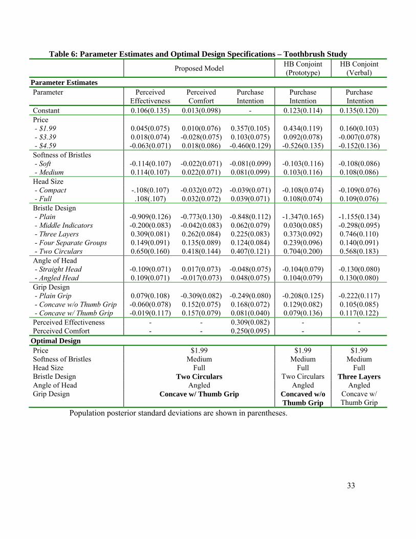
In Table 6, we provide the parameter estimates from the proposed model, the prototype-

based HB conjoint model, and the verbal HB conjoint model. Interestingly, the proposed model

estimates suggest that, at the population level, price does not play an important role in

consumer’s perceptions of whether a toothbrush is effective or comfortable to use. In contrast,

price has a strong direct impact on purchase intention with a higher price being less preferred.

The individual-specific intercepts seem to explain more variance in perceived effectiveness than

perceived comfort. At the population level, consumers perceive a medium, full, angled head

toothbrush with a two-circular bristle design to be effective. With regard to perceived comfort, it

is clear that a two-circular bristle design and a concave handle with thumb grip are considered as

the most comfortable to use. Partially mediating the effects of the objective attributes on

purchase intention, both subjective characteristics play an important role in consumer’s purchase

decision, with perceived effectiveness valued slightly more than perceived comfort. The last two

columns in Table 6 provide the model estimates from the prototype-based HB conjoint model in

Condition 1 and the verbal HB conjoint model in Condition 2.

<Insert Table 6 about here>

Next, we compare the optimal designs predicted by the three models (Table 6). The

optimal designs predicted by the three models vary in bristle designs and grip designs. This is

quite intuitive because the bristle and grip design of a toothbrush exerts an indirect influence on

purchase likelihood through perceived effectiveness and comfort. The absence of such effects in

the traditional conjoint models led to the selection of possibly suboptimal product designs. It is

not surprising that the optimal products suggested by the three models are all low priced.

Because price does not have any impact on perceived effectiveness or comfort of the toothbrush,

consumers always prefer a cheaper toothbrush given everything else being equal.

28

CONCLUSIONS

In this paper, we have developed a formal model to incorporate the impact of the

subjective characteristics in new product design. Through two empirical applications, we have

demonstrated that the traditional conjoint models may not be sufficiently information-rich for

product designers. With the creation of several customer-ready prototypes and the collection of

additional data on subjective characteristics, our proposed model can help the product designer

to better understand: 1) the causal relationships between the objective attributes and the

subjective characteristics at the individual and aggregate levels; and 2) how the objective

attributes and the subjective characteristics jointly influence consumer’s purchase decision. Such

diagnostic information can be very useful for the manager to properly position and promote the

new product in the marketplace. Furthermore, our model provides an actionable procedure so

that the product designers can take into account the subjective characteristics in predicting

consumers’ purchase intentions for out-of-sample product alternatives. As a result, our model

offers the product designer a more accurate out-of-sample prediction as compared to the

traditional conjoint models.

Historically, the qualitative aspects of the products have not received much attention in

the quantitative modeling of new product design literature. From a theoretical perspective, one

particular obstacle is that consumers’ perceptions of the subjective characteristics often depend

on a complex set of factors that can be different for different individuals. An additional modeling

effort is needed to deal with this complexity. Our hierarchical Bayesian structural equation

model provides a feasible solution to this problem. From the perspective of implementation, the

cost of developing customer-ready prototypes has been the main concern of using prototypes in

product development (Srinivasan et al. 1997). We suggest that there are effective ways of

29

producing the prototype stimuli. A collection of the existing products on the market can be used

to form the basis of the prototype pool. Products with new features can be generated at a

relatively low cost as alterations of existing products. Consequently, we believe that the

methodology introduced in this paper is amenable to practical application.

A limitation of our research is that the highly fractionated main-effects designs that we

employed limited our ability to address potential interaction effects among the objective

attributes. Specifically, several simulation studies employing our fractional main effects designs

indicated that our model could not uncover interaction effects after main effects were removed.

This limitation could be overcome by employing other designs, which would involve presenting

consumers with more prototypes. Another possible limitation of our proposed data collection

approach is that it may not be feasible when there are large numbers of attributes or when

prototypes are expensive to produce. In such situations, virtual reality representations (Dahan

and Srinivasan 2000) may be considered as substitutes for physical prototypes. Finally, if

prototypes or virtual reality representations are used in various choice scenarios, a discrete

choice model could be built into our conceptual framework. In this case, the general model

would be similar to the model presented in Ashok et al. (2002) with the subjective characteristics

defined as functions of the objective attributes and individual-specific effects. Future research

might investigate the applicability of our approach to cases with interaction effects, high

numbers of attributes, and choice-based designs.

30

Table 1: Model Comparisons – Power Tool Study Proposed Model Subjective Only HB Conjoint (Model 1) (Model 2) (Model 3) In-Sample Fit - Pseudo R2 0.615 0.565 0.523 - DIC 1658.270 1669.337 1770.040 - RMSD 0.330 0.358 0.405 Predictive Power - MAE 10.79% - 12.41% - RMSE 12.13% - 15.58%

Table 2: Robustness Check in Predictive Validity – Power Tool Study Proposed Model HB Conjoint Predictive

Power Average Average Range of Improvement

in Percentage - MAE 11.45% 13.39% 10.23% - 17.65% - RMSE 12.53% 15.52% 14.69% - 22.14%

31

Table 3: Parameter Estimates and Optimal Design Specifications – Power Tool Study Proposed Model HB Conjoint Model

Parameter Estimates Parameter Perceived

Power Perceived Comfort

Purchase Intention

Purchase Intention

Constant 0.053(0.162) 0.169(0.123) - 0.187(0.172) Shape - Rear Motor -.0.159(0.109) 0.051(0.097) -0.255(0.096) -0.253(0.113) - Ultimate Body Grip -0.120(0.109) -0.008(0.092) -0.037(0.090) -0.056(0.100) - Large than UBG 0.279(0.107) -0.043(0.132) 0.292(0.128) 0.309(0.151) Switch Type - Top Slider -0.070(0.096) -0.294(0.097) -0.039(0.094) -0.188(0.106) - Side Slider -0.017(0.096) -0.292(0.100) -0.011(0.101) -0.226(0.112) - Paddle 0.011(0.093) 0.130(0.095) 0.065(0.096) 0.234(0.105) - Trigger 0.076(0.181) 0.456(0.183) -0.015(0.183) 0.180(0.181) Weight - 4.5 lbs -0.145(0.109) 0.109(0.090) 0.068(0.091) 0.106(0.109) - 5.5 lbs 0.145(0.109) -.109(0.090) -0.068(0.091) -0.106(0.109) Price - $79 -0.134(0.092) -0.001(0.094) 0.105(0.091) -0.101(0.101) - $99 0.013(0.090) 0.016(0.089) -0.018(0.094) -0.105(0.100) - $129 0.120(0.082) -0.015(0.076) -0.087(0.130) 0.206(0.135) Perceived Power - - 0.207(0.095) - Perceived Comfort - - 0.726(0.094) -

Optimal Design Shape Larger than UBG Larger than UBG Switch Type Trigger Paddle Weight 4.5 lbs 4.5 lbs Price $129 $129

Population posterior standard deviations are shown in parentheses.

32

Table 4: Model Comparisons – Toothbrush Study Condition 1: Prototype-Based Condition 2: Verbal Proposed Model Subjective Only HB Conjoint HB Conjoint (Model 1) (Model 2) (Model 3) (Model 4) In-Sample Fit - Pseudo R2 0.658 0.449 0.587 0.541 - DIC 3151.030 3681.814 3279.380 - - RMSD 0.329 0.497 0.410 0.469 Predictive Power - Hit Rate 75.00% - 65.48% 60.94% - MAE 9.26% - 11.03% 14.94% - RMSE 11.74% - 13.31% 16.55%

Table 5: Robustness Check in Predictive Validity – Toothbrush Study Condition 1: Prototype-Based Condition 2: Verbal

Proposed Model HB Conjoint HB Conjoint Predictive Power Average Average

Range of Improvement in Percentage Average

Range of Improvement in Percentage

- MAE 10.15% 12.28% 13.46%-21.99% 14.85% 24.23%-38.05% - RMSE 12.39% 14.56% 10.92%-18.43% 17.76% 23.16%-36.43%

33

Table 6: Parameter Estimates and Optimal Design Specifications – Toothbrush Study Proposed Model HB Conjoint

(Prototype) HB Conjoint

(Verbal) Parameter Estimates Parameter Perceived

Effectiveness Perceived Comfort

Purchase Intention

Purchase Intention

Purchase Intention

Constant 0.106(0.135) 0.013(0.098) - 0.123(0.114) 0.135(0.120) Price - $1.99 0.045(0.075) 0.010(0.076) 0.357(0.105) 0.434(0.119) 0.160(0.103) - $3.39 0.018(0.074) -0.028(0.075) 0.103(0.075) 0.092(0.078) -0.007(0.078) - $4.59 -0.063(0.071) 0.018(0.086) -0.460(0.129) -0.526(0.135) -0.152(0.136) Softness of Bristles - Soft -0.114(0.107) -0.022(0.071) -0.081(0.099) -0.103(0.116) -0.108(0.086) - Medium 0.114(0.107) 0.022(0.071) 0.081(0.099) 0.103(0.116) 0.108(0.086) Head Size - Compact -.108(0.107) -0.032(0.072) -0.039(0.071) -0.108(0.074) -0.109(0.076) - Full .108(.107) 0.032(0.072) 0.039(0.071) 0.108(0.074) 0.109(0.076) Bristle Design - Plain -0.909(0.126) -0.773(0.130) -0.848(0.112) -1.347(0.165) -1.155(0.134) - Middle Indicators -0.200(0.083) -0.042(0.083) 0.062(0.079) 0.030(0.085) -0.298(0.095) - Three Layers 0.309(0.081) 0.262(0.084) 0.225(0.083) 0.373(0.092) 0.746(0.110) - Four Separate Groups 0.149(0.091) 0.135(0.089) 0.124(0.084) 0.239(0.096) 0.140(0.091) - Two Circulars 0.650(0.160) 0.418(0.144) 0.407(0.121) 0.704(0.200) 0.568(0.183) Angle of Head - Straight Head -0.109(0.071) 0.017(0.073) -0.048(0.075) -0.104(0.079) -0.130(0.080) - Angled Head 0.109(0.071) -0.017(0.073) 0.048(0.075) 0.104(0.079) 0.130(0.080) Grip Design - Plain Grip 0.079(0.108) -0.309(0.082) -0.249(0.080) -0.208(0.125) -0.222(0.117) - Concave w/o Thumb Grip -0.060(0.078) 0.152(0.075) 0.168(0.072) 0.129(0.082) 0.105(0.085) - Concave w/ Thumb Grip -0.019(0.117) 0.157(0.079) 0.081(0.040) 0.079(0.136) 0.117(0.122) Perceived Effectiveness - - 0.309(0.082) - - Perceived Comfort - - 0.250(0.095) - -

Optimal Design Price $1.99 $1.99 $1.99 Softness of Bristles Medium Medium Medium Head Size Full Full Full Bristle Design Two Circulars Two Circulars Three Layers Angle of Head Angled Angled Angled Grip Design Concave w/ Thumb Grip Concaved w/o

Thumb Grip Concave w/ Thumb Grip

Population posterior standard deviations are shown in parentheses.

34

Figure 1: View of Product Evaluation

Objective Attributes

Purchase Intention

Idiosyncrasy Subjective

Characteristics

Indicator Variable 1

Indicator Variable K

… Indicator Variable 2

35

References Addelman, Sidney (1962), “Symmetrical and Asymmetrical Fractional Factorial Plans”,

Technometrics, Vol. 4, February, 47-58. Ansari, Asim, Kamel Jedidi, and Sharan Jagpal (2000), “A Hierarchical Bayesian Methodology for

Treating Heterogeneity in Structural Equation Models”, Marketing Science, Vol. 19, No. 4, 328-347.

Ashok, Kalidas, William R. Dillon, and Sophie Yuan (2002), “Extending Discrete Choice Models to

Incorporate Attitudinal and Other Latent Variables”, Journal of Marketing Research, Vol. 39, No. 1, 31-46.

Bollen, Kenneth A. (1989), Structural Equations with Latent Variables, John Wiley & Sons Inc.,

New York, USA. Dahan, Ely and V. Srinivasan (2000), “The Predictive Power of Internet-Based Product Concept

Testing using Visual Depiction and Animation”, Journal of Product Innovation Management, Vol. 17, No. 2, 99-109.

Gelman, A., X. L. Meng, and H. S. Stern (1996), “Posterior Predictive Assessment of Model Fitness

via Realized Discrepancies”, Statistica Sinica, Vol. 6, 733-807. Griffin, Abbie and John R. Hauser (1993), “The Voice of the Customer”, Marketing Science, Vol.

12, No. 1, 1-27. Gupta, P. B. and Kenneth R. Lord (1995), “Identification of Determinant Attributes of Automobiles:

Objective Analogues of Perceptual Construct”, The Journal of Marketing Management, Spring/Summer, 21-29.

Hauser, John R. and Don Clausing (1988), “The House of Quality”, Harvard Business Review, May-

June, 63-73. Huber, Joel and John McCann (1982), “The Impact of Inferential Beliefs on Product Evaluations”,

Journal of Marketing Research, Vol. 19, No. 3, 324-333. Jedidi, Kamel, Sharan Jagpal, and Puneet Manchanda (2003), “Measuring Heterogeneous

Reservation Prices for Product Bundles”, Marketing Science, Vol. 22, No. 1, 107-130. Lawton, Christopher (2006), “Consumer Demand and Growth in Laptops Leave Dell Behind”, The

Wall Street Journal, August 30. Mahajan, Vijay, Paul E. Green, and Stephen M. Goldberg (1982), “A Conjoint Model for Measuring

Self- and Cross-Price/Demand Relationships”, Journal of Marketing Research, Vol. 19, No. 3, 334-342.

Moore, William L., Jason Gray-Lee and Jordan J. Louviere (1998), "A Cross-Validity

36

Comparison of Conjoint Analysis and Choice Models at Different Levels of Aggregation," Marketing Letters, Vol. 9, No. 2, 195-208.

Mulenburg, Gerald M. (2004), “From NASA: Don’t Overlook the Value of Prototype-as-Design in

Developing Your New Product”, Vision, Vol. XXVIII, No. 4, October, 8-10. Narasimhan, Chakravarthi and Subrata K. Sen (1992), “Measuring Quality Perceptions”, Marketing

Letters, Vol. 3, No. 2, 147-156. Neslin, Scott A. (1981), “Linking Product Features to Perceptions: Self-Stated Versus Statistically

Revealed Important Weight”, Journal of Marketing Research, Vol. 18, No. 1, 80-86. Rao, Akshay R. and Kent B. Monroe (1989), “The Effect of Price, Brand Name, and Store Name

on Buyers’ Perceptions of Product Quality: An Integrative Review”, Journal of Marketing Research, Vol. 26, August, 351-357.

----- and ----- (1996), “Causes and Consequences of Price Premiums”, The Journal of Business,

Vol.69, No.4, 511-535. Rossi, Peter E. and Greg M. Allenby (2003), “Bayesian Statistics and Marketing”, Marketing

Science, Vol. 22, No. 3, 304-328. Sawtooth CVA User’s Manual (2002), Sawtooth Software, Inc., Sequim, Washington. Sörbom, D. (1981), “Structural Equation Models with Structured Means”, K.G. Joreskog, H. Wold,

eds., Systems under Indirect Observation: Causality, Structure, and Prediction, Amsterdam, Netherlands, 183-195.

Spiegelhalter, David J., Nicola G. Best, Bradley P. Carlin, and Angelika van der Linde (2002),

“Bayesian Measure of Model Complexity and Fit”, Journal of Royal Statistics Society, Vol. 64, No. 4, 583-639.

Srinivasan, V., William S. Lovejoy, and David Beach (1997), “Integrated Product Design for

Marketability and Manufacturing”, Journal of Marketing Research, Vol. 34, No. 1, 154-163. Tybout, Alice M. and John R. Hauser (1981), “A Marketing Audit Using a Conceptual Model of

Consumer Behavior: Application and Evaluation”, Journal of Marking, Vol. 45, No. 3, 82-101.

Yamamoto, Mel and David R. Lambert (1994), “The Impact of Product Aesthetics on the Evaluation

of Industrial Products”, Journal of Product Innovation Management, Vol. 11, No. 4, 309-324.

Yung, Yiu-Fai (1997), “Finite Mixtures in Confirmatory Factor-Analysis Models”, Psychometrika,

Vol. 62, No. 3, 297-330. Appendix:

37

A. Steps in Markov Chain Monte Carlo Simulation Our MCMC procedure is carried out by sequentially generating draws from the following

distributions: 1. Generate the loading matrixΛ

The loading matrix is a patterned matrix with both fixed and free elements. Some of the fixed elements are zero and others are one, depending on the model setup and the identification requirement. Let jλ denote the thj column vector of the free elements in the loading matrix, isv~ be

the vector of indicator variables that correspond to these factor loadings, and ijθ~ be the

corresponding sub-matrix of the measurement errors. The full conditional distribution of jλ is given by:

( ) ( ) ( )jis

S

s

N

ij fvff λλ *~*

11ΠΠ==

∝ (A1)

Where )~'),((~*~ijjijjisijijjis xbMVNv θλλδλ +Δ+ and the prior distribution of jλ is given as

follows. For each element kjλ in jλ , we let 12 −×= kjkj ldλ with ),(~ οιBetaldkj . The transformed Beta distribution has an [ ]1,1− interval for the factor loadings. We set 2=ι and

2=ο to ensure diffuse but proper priors. 2. Generate the factor scores isz

( ) ),(*iis zzis MVNzf Δ= ω (A2)

The mean iszω and the variance-covariance matrix

izΔ come from two data sources. The first data source is the measurement equation isisiis εzΛv += . The second data source is from the structural equation issiis μxBδz i ++= . Therefore, the full conditional distribution for isz can be

written as )Δ,ω(iis zzMVN , where ]vΘ'Λ)xBδ(Δ[Δω 11

isisiiizz iis

−− ++= and ΛΘ'ΛΔΔ 111 −− += ii-

iz.

3. Generate the measurement errors isε ( ) ( ) ( )isisis fff ε*v*ε ∝ (A3)

Where )'),xBδ(Λ(~*v iiisiiis MVN Θ+ΛΛΔ+ ),0(~ε iis MVN Θ

4. Generate iδ

( ) ( ) ( )iis

S

si fff δδ *v*

1Π=

∝ (A4)

Where ),(~ Σκδ MVNi 5. Generate ''b,...,'b,'bB 21 iJiii =

)B()*v()*B(1

iis

S

si fff Π

=

∝ (A5)

Where )D,β(~b jjij MVN for Jj ,...,1= 6. Generate isμ

)μ()*v()*μ( isisis fff ∝ (A6)

38

Where )Δ,0(~μ iis MVN 7. Generate iii γ,Aη =

)η()*v()*()*η(1

iisis

S

si ffyff Π

=

∝ (A7)

Where )γΔγ,x)BγA(δγ(~* 2'eiiiisiiiiiis MVNy σ+++

),(~ Ωϕη MVNi 8. Generate ise

)()*v()*()*( isisisis effyfef ∝ (A8)

Where ),0(~ 2eis Ne σ

9. Generate )( iik diag Θ=θ for Kk ,...,1=

Let iskv denote the corresponding indicator variable, kλ~ be the corresponding factor

loading, and iskz represent the corresponding factor score. The full conditional distribution for

ikθ ( Kk ,...,1= ) is:

)])~(21[,

2()*( 12

1

−

=

−++= ∑ iskk

S

siskkkik zvSIGf λψςθ (A9)

10. Generate iΔ

)][,()*( 1'

1

11 −

=

−− ∑++=Δ is

S

sisi RSWf μμρ (A10)

11. Generate 2eσ

)])zx(21[,

2()*( 12

1 1

12 −

= =

− −−+×

+= ∑∑ isisi

N

i

S

siseee AySNIGf γψϖσ (A11)

Where 2=eϖ and 1=ψ are the priors of the Inverse Gamma distribution. 12. Generate the hyper-parameter kς for Kk ,...,1=

)()*()*(1

kik

N

ik fff ςθς Π

=

∝ (A12)

Where the prior distribution is defined as ),0(~)log( kk N τς . We use the log-transformation to ensure a positive sign of kς . We set 100=kτ . 13. Generate the hyper-parameter kψ for Kk ,...,1=

)][,()*( 1

1

11 −

=

−− ∑++=N

iikkkkk hNgIGf θςψ (A13)

Where the prior distribution is defined as ),(~ kkk hgIGψ . We set 5.0=kg and 1=kh to ensure diffuse but proper priors. 14. Generate the hyper-parameter ρ

)()*()*( 1

1ρρ fff i

N

i

−

=

Δ∝Π (A14)

Where the prior distribution is defined as JN >ρτρ ρ ),0(~)log( . This prior distribution

39

is selected based on two criteria: 1) ρ has to be a positive number; and 2) ρ needs to be greater than the dimension of the matrix J . We set 100=ρτ . 15. Generate the hyper-parameter R

)R(*)()*R( 11

1

1 −−

=

Δ∝Π fff i

N

i

- (A15)

Where the prior distribution is defined as ))R(,(~R 1000

1 −− ρρW with 50 =ρ and IR0 = ( I is a JJ × identity matrix).

16. Generate the hyper-parameter κ )()*( κκϑκ Γ= ,MVNf (A16)

Where

⎥⎥⎥⎥

⎦

⎤

⎢⎢⎢⎢

⎣

⎡

Γ+−

⎟⎠⎞

⎜⎝⎛

−Σ

Γ= −=− ∑

κκκκ

δϑ r

)1(112

1

NN

N

ii

and 11

10 )

1( −

−− ⎟

⎠⎞

⎜⎝⎛

−Σ

+Γ=ΓNκκ . We set the priors

as 0=κr and I1000 =Γκ ( I is a JJ × identity matrix). 17. Generate the hyper-parameter Σ

)R)')((,)1((*)( 02

01

Σ=

Σ− +−−+−=Σ ∑ κδκδρ i

N

iiNWf (A17)

Where the priors are set as 50 =Σρ and I5R 0 =Σ ( I is a JJ × identity matrix). 18. Generate the hyper-parameter jβ for Jj ,...,1=

),()*(jj

MVNf j ββϑβ Γ∝ (A18)

Where

⎥⎥⎥⎥

⎦

⎤

⎢⎢⎢⎢

⎣

⎡

Γ+

⎟⎟⎟⎟

⎠

⎞

⎜⎜⎜⎜

⎝

⎛

⎟⎟⎠

⎞⎜⎜⎝

⎛Γ= −=

− ∑0

10

1

1

jjjjr

N

b

ND

N

iij

jββββϑ and

111

0

−−−

⎟⎟

⎠

⎞

⎜⎜

⎝

⎛⎟⎟⎠

⎞⎜⎜⎝

⎛+Γ=Γ

NDj

jj ββ . We set the

priors as 00 =jrβ and I1000 =Γ

jβ ( I is a MM × identity matrix).

19. Generate the hyper-parameter jD for Jj ,...,1=

),()*( 1jj DDj RWDf ρ=− (A19)

Where 0jj DD N ρρ += and 01

R)')((Rjj Djijj

N

iijD bb +−−=∑

=

ββ . We set the diffuse but

proper priors as 100 =jDρ and I10R 0 =jD ( I is a MM × identity matrix). 20. Generate the hyper-parameter φ

),(*)( ϕϕϑφ Γ= MVNf (A20)

40

Where

⎥⎥⎥⎥

⎦

⎤

⎢⎢⎢⎢

⎣

⎡

Γ+⎟⎠⎞

⎜⎝⎛ ΩΓ= −=

− ∑0

10

11

rϕϕϕϕ

ηϑ

NN

N

ii

and11

10

−−−

⎟⎟⎠

⎞⎜⎜⎝

⎛⎟⎠⎞

⎜⎝⎛ Ω+Γ=Γ

Nϕϕ . We set the priors as

0r 0 =ϕ and I1000 =Γϕ . 21. Generate the hyper-parameter Ω

)R)'φη)(φη(,(*)( 01

01

Ω=

Ω− +−−+=Ω ∑ i

N

iiNWf ρ (A21)

Where the priors are set at 150 =Ωρ and I15R 0 =Ω .

B. Supplemental Information on Study One: The Design of a Handheld Power Tool In this study, the objective attributes were selected based on: 1) their importance to the

end users, and 2) their relevance to the subjective characteristics. For example, motor type was not included because its selection does not influence the emotional or physical appeal of the tool. However, the limitation of excluding motor power as an objective attribute is that the proposed model’s incremental goodness-of-fit and predictive power over the benchmark conjoint model may be inflated to some extent.

Our experimental design among the calibration profiles provides a D-efficiency of 74.34.

The D-efficiency index is calculated using the formula MXXS

/11)'(

100−

with S representing the

number of calibration profiles, X being the design matrix using effects-type dummy variable coding, and M being the dimension of the design matrix X (Kuhfeld, Tobias, and Garratt 1994).

The average rating of each prototype on perceived power ranged from 3.491 (prototype #5) to 5.292 (prototype #2) and, on perceived comfort, it varied from 2.768 (prototype #3) to 5.289 (prototype #9) on a 7-point scale. This indicates that there was a considerable amount of variation in perceived power and perceived comfort across these prototypes.

The factor loadings from the proposed model are presented in the third column of Table B1. In order to evaluate how well the values of the objective attributes and the posterior distribution of the relevant model parameters can predict the actual subjective ratings, we calculated the Pseudo R2 measures (last column of Table B1). In general, our findings suggest that the indicator variables were reliable measures of the underlying latent constructs and our model was able to explain a reasonable amount of variance in the subjective ratings.

Table B1: Indicator Variable Estimates – Power Tool Study Latent Construct Indicator Factor Loading Pseudo R2 Perceived Power pwr1 1 0.638

pwr2 0.728 (0.052) 0.478 pwr3 0.745 (0.051) 0.512

Perceived Comfort cft1 1 0.548 cft2 0.657 (0.051) 0.402 cft3 0.656 (0.053) 0.332 cft4 0.677 (0.050) 0.430

Posterior standard deviations are in parentheses.

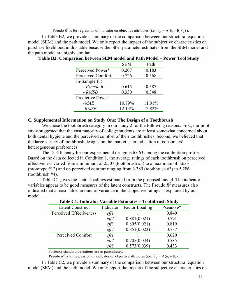
41

Pseudo R2 is for regression of indicator on objective attributes (i.e. )xBδ(Λv siiis += ). In Table B2, we provide a summary of the comparison between our structural equation

model (SEM) and the path model. We only report the impact of the subjective characteristics on purchase likelihood in this table because the other parameter estimates from the SEM model and the path model are highly similar.

Table B2: Comparison between SEM model and Path Model – Power Tool Study SEM Path

Perceived Power* 0.207 0.183 Perceived Comfort 0.726 0.568 In-Sample Fit - Pseudo R2 0.615 0.587 - RMSD 0.330 0.348 Predictive Power -MAE 10.79% 11.01% -RMSE 12.13% 12.82%

C. Supplemental Information on Study One: The Design of a Toothbrush

We chose the toothbrush category in our study 2 for the following reasons. First, our pilot study suggested that the vast majority of college students are at least somewhat concerned about both dental hygiene and the perceived comfort of their toothbrushes. Second, we believed that the large variety of toothbrush designs on the market is an indication of consumers’ heterogeneous preferences.

The D-Efficiency for our experimental design is 65.63 among the calibration profiles. Based on the data collected in Condition 1, the average ratings of each toothbrush on perceived effectiveness varied from a minimum of 2.507 (toothbrush #5) to a maximum of 5.633 (prototype #12) and on perceived comfort ranging from 3.389 (toothbrush #3) to 5.286 (toothbrush #4).

Table C1 gives the factor loadings estimated from the proposed model. The indicator variables appear to be good measures of the latent constructs. The Pseudo R2 measures also indicated that a reasonable amount of variance in the subjective ratings is explained by our model.

Table C1: Indicator Variable Estimates – Toothbrush Study Latent Construct Indicator Factor Loading Pseudo R2

Perceived Effectiveness eff1 1 0.849 eff2 0.881(0.021) 0.791 eff3 0.895(0.021) 0.819 eff4 0.851(0.023) 0.737

Perceived Comfort cft1 1 0.620 cft2 0.705(0.034) 0.585 cft3 0.573(0.039) 0.433

Posterior standard deviations are in parentheses. Pseudo R2 is for regression of indicator on objective attributes (i.e. )xBδ(Λv siiis +=

In Table C2, we provide a summary of the comparison between our structural equation model (SEM) and the path model. We only report the impact of the subjective characteristics on

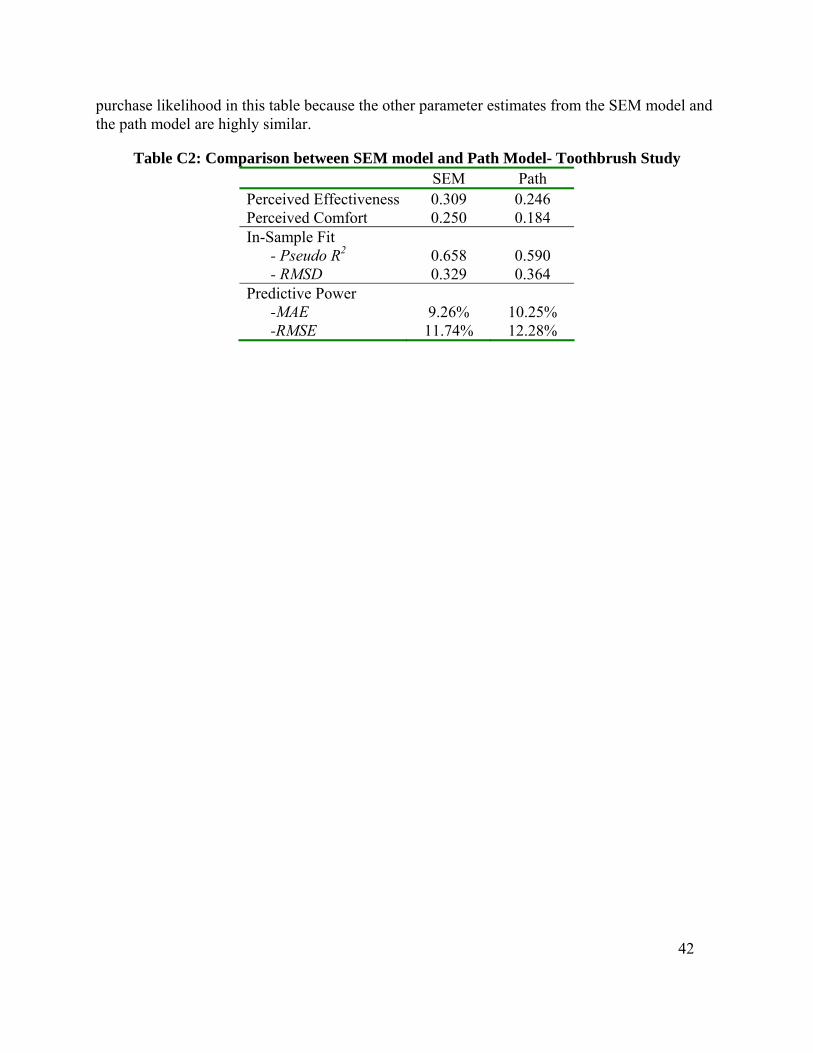
42

purchase likelihood in this table because the other parameter estimates from the SEM model and the path model are highly similar.

Table C2: Comparison between SEM model and Path Model- Toothbrush Study SEM Path Perceived Effectiveness 0.309 0.246 Perceived Comfort 0.250 0.184 In-Sample Fit - Pseudo R2 0.658 0.590 - RMSD 0.329 0.364 Predictive Power -MAE 9.26% 10.25% -RMSE 11.74% 12.28%