Incorporating Irregular Nonlinear Waves in Coupled

Simulation of Offshore Wind Turbines

Puneet Agarwal∗

Stress Engineering Services, Houston, TX 77041

Lance Manuel†

Department of Civil, Architectural, and Environmental Engineering

The University of Texas, Austin, TX 78712

Design of an offshore wind turbine requires estimation of loads on its rotor, tower andsupporting structure. These loads are obtained by time-domain simulations of the coupledaero-servo-hydro-elastic model of the wind turbine. Accuracy of predicted loads dependson assumptions made in the simulation models employed, both for the turbine and for theinput wind and wave conditions. Currently, waves are simulated using a linear irregularwave theory, which is not appropriate for nonlinear waves in shallow water depths, wherewind farms are typically sited. The present study investigates the use of irregular nonlinear(second-order) waves for estimating loads on the support structure (monopile) of an offshorewind turbine. We present the theory for the irregular nonlinear model and incorporate itin the commonly used wind turbine simulation software, FAST, which had been developedby National Renewable Energy Laboratory (NREL), but which had the modeling capabilityonly for irregular linear waves. We use an efficient algorithm for computation of nonlinearwave elevation and kinematics, so that a large number of time-domain simulations, whichare required for prediction of long-term loads using statistical extrapolation, can easily beperformed. To illustrate the influence of the alternative wave models, we compute loadsat the base of the monopile of the NREL 5MW baseline wind turbine model using linearand nonlinear irregular wave models. We show that for a given environmental condition(i.e., the mean wind speed and the significant wave height), extreme loads are larger whencomputed using the nonlinear wave model. We then compute long-term loads, which arerequired for a design load case according to the International Electrotechnical Commissionguidelines. We show that 20-year long-term loads can be significantly higher when thenonlinear wave model is used.

I. Introduction

Offshore wind energy is becoming an important part of the overall energy mix in Europe and has greatpotential within the United States and other parts of the world. The potential for offshore wind powerin the United States, in water depths less than 30 meters where current fixed-bottom support structuretechnologies can be used, is about 98 GW.1 Europe has a target of generating about 12% of its electricityfrom wind by the year 2020, of which about one-third, or about 30 GW (gigawatts), is expected to comefrom offshore projects.2, 3 To meet such demand, it is important to develop appropriate simulation tools fordesign of offshore wind turbines.

Response of an offshore wind turbine to the input wind and waves, both of which are stochastic in nature,is estimated using coupled aero-servo-hydro-elastic simulation in time domain. Such time-domain simulationsare also used to obtain the data on load extremes, which are needed for calculation of long-term (for a returnperiod of 20 or 50 years) extreme loads using the statistical extrapolation method as recommended by theIEC 61400-3 standard4 from International Electrotechnical Commission (IEC). The accuracy of the turbineresponse depends on the proper modeling and interfacing of various parts of the physics (aeroelasticity,

∗Senior Analyst†Associate Professor

1 of 16

American Institute of Aeronautics and Astronautics

48th AIAA Aerospace Sciences Meeting Including the New Horizons Forum and Aerospace Exposition4 - 7 January 2010, Orlando, Florida

AIAA 2010-996

Copyright © 2010 by Puneet Agarwal and Lance Manuel. Published by the American Institute of Aeronautics and Astronautics, Inc., with permission.

dynamics, control systems etc) of an offshore wind turbine, as well as on the appropriate modeling of theincident wind and waves. In this paper, we exclusively focus on how alternate wave models influence theturbine response.

The current practice to model waves on offshore wind turbines is limited to linear irregular waves, whichare not an accurate representation of waves in shallow waters where offshore wind turbines are most commonlysited. In shallow waters, waves are generally nonlinear in nature, therefore we attempt to incorporate anonlinear irregular wave model in the coupled aero-servo-hydro-elastic simulation of offshore wind turbines.

Among several nonlinear irregular wave models available in the literature, the one that has been recom-mended by offshore guidelines5 and that has been increasingly applied to a variety of problems in recentyears5–8 is the second-order nonlinear irregular wave model developed by Sharma and Dean9 for finite waterdepths. This second-order nonlinear irregular wave model is based on the solution of the Laplace equationin velocity potential, associated with nonlinear boundary conditions, using a second-order perturbation ex-pansion of the relevant variables (velocity potential and sea surface elevation) and a Taylor series expansionof nonlinear boundary conditions about the free surface. Such an approach was first presented by Longuet-Higgins10 and Hasselmann11 for infinite water depths. Since its introduction in 1979, the second-ordernonlinear irregular wave model developed by Sharma and Dean has been studied by several researchers. Huand Zhao,12 Langley,13 Longuet-Higgins14 and Forristall,15 among others, investigated the statistical proper-ties (skewness in particular) of this nonlinear irregular wave model. Forristall16 compared various stretchingtechniques for calculating wave kinematics above the mean sea level. Due to such maturity of this nonlinearirregular wave model and because of its theoretical basis (as distinct from some semi-empirical models, suchas the New Wave model,17 the constrained New Wave model18 and a hybrid wave model19), and also dueto its computational efficiency for simulations (as distinct from more realistic though computationally veryexpensive models based on Boussinesq theory20, 21), we will use this second-order nonlinear irregular wavemodel, as developed by Sharma and Dean,9 to simulate nonlinear irregular waves in shallow water depthsfor offshore wind turbine loads predictions.

The outline of this paper is as follows: we first present an overview of the hydrodynamics—employingthe currently used linear irregular wave model—in the coupled simulation of offshore wind turbines. Wepresent the theoretical formulation of the second-order nonlinear irregular wave model. We limit our focusto unidirectional (long-crested) waves. We then present a detailed procedure, which we have incorporatedin the turbine response simulation software, FAST,22 for efficient simulation of the sea surface elevation andthe water particle kinematics process based on the nonlinear irregular wave model. We use a utility-scale5MW offshore wind turbine model developed at the National Renewable Energy Laboratory (NREL)23 tocompare turbine response (mainly the fore-aft tower bending moment at the mudline) due to linear andnonlinear irregular waves. we compute the turbine response for a representative environmental state, andshow that when nonlinear waves are used, turbine loads can be larger and tower dynamics can be influencedto some extent as well. We finally show that long-term loads are significantly larger with nonlinear waves,and therefore, it is important to use nonlinear wave model in the design of offshore wind turbines.

II. Hydrodynamics in Coupled Simulation of Offshore Wind Turbines

Structural response of wind turbines—both onshore and offshore—in the time domain is analyzed usingcoupled aero-servo-hydro-elastic simulation programs. One such program is FAST (Fatigue, Aerodynamics,Structures and Turbulence),22 developed at the National Renewable Energy Laboratory (NREL). FASTis a medium-complexity program that models a wind turbine as a combination of rigid and flexible bodieswherein flexible beam elements (representing the blades and the tower) are formulated in terms of generalizedcoordinates. Aerodynamic forces on the rotating blades of a horizontal-axis wind turbine are commonlycomputed using the blade element momentum theory.24 FAST models various control systems includingblade and pitch control, yaw control, and high-speed shaft brake control. FAST uses irregular linear wavemodel with Morison’s equation to compute hydrodynamic loads for offshore wind turbines. Perhaps themost important aspect of the FAST program is the proper interfacing of various parts of the physics—aeroelasticity, dynamics, control systems, hydrodymaics, etc—of an offshore wind turbine. Without suchcoupling, it is not possible to accurately assess the response of wind turbines. We next discuss hydrodynamiccalculations in FAST, while highlighting its limitations to model shallow water waves.

2 of 16

American Institute of Aeronautics and Astronautics

Wave Spectrum, S(ωm)

Random Amplitudes and Phases

Am ∼ Rayleigh, E[A2m] = 2S(ωm)∆ω

φm ∼ Uniform[0, 2π]

Random Seeds

Fourier Coefficients for Sea Surface Elevation

X(ωm) = Am exp(−iφm)

Fourier Coefficients for Wave Kinematics

Xu(h, z, ωm) = gkm

ωm

cosh(km(h+z))cosh(kmh) X(ωm)

Xu(h, z, ωm) = −Xu(h, z, ωm)ωm

Time-series of Wave Elevation and Kinematics

Sea Surface Elevation: η1(tp) = ℜ[ IFFT(X(ωm))]

Particle Velocity: u1(tp, z) = ℜ[ IFFT (Xu(ωm))]

Particle Acceleration: u1(tp, z) = ℑ[ IFFT(Xu(ωm))]

Hydrodynamic Loads

f = 12CDρD(u1 − q)|u1 − q|

+[

CMπD2

4 ρu1 − (CM − 1)πD2

4 ρq]

Support structure

motion: q, q, q

Hydrodynamic

loads

Aero-Servo-Hydro-Elastic Simulator, FAST

IrregularLinearWaveSim

ulation

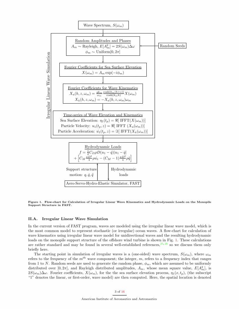
Figure 1. Flow-chart for Calculation of Irregular Linear Wave Kinematics and Hydrodynamic Loads on the MonopileSupport Structure in FAST.

II.A. Irregular Linear Wave Simulation

In the current version of FAST program, waves are modeled using the irregular linear wave model, which isthe most common model to represent stochastic (or irregular) ocean waves. A flow-chart for calculation ofwave kinematics using irregular linear wave model for unidirectional waves and the resulting hydrodynamicloads on the monopile support structure of the offshore wind turbine is shown in Fig. 1. These calculationsare rather standard and may be found in several well-established references,25, 26 so we discuss them onlybriefly here.

The starting point in simulation of irregular waves is a (one-sided) wave spectrum, S(ωm), where ωm

refers to the frequency of the mth wave component; the integer, m, refers to a frequency index that rangesfrom 1 to N . Random seeds are used to generate the random phase, φm, which are assumed to be uniformlydistributed over [0, 2π], and Rayleigh distributed amplitudes, Am, whose mean square value, E[A2

m], is2S(ωm)∆ω. Fourier coefficients, X(ωm), for the the sea surface elevation process, η1(x, tp), (the subscript“1” denotes the linear, or first-order, wave model) are then computed. Here, the spatial location is denoted

3 of 16

American Institute of Aeronautics and Astronautics

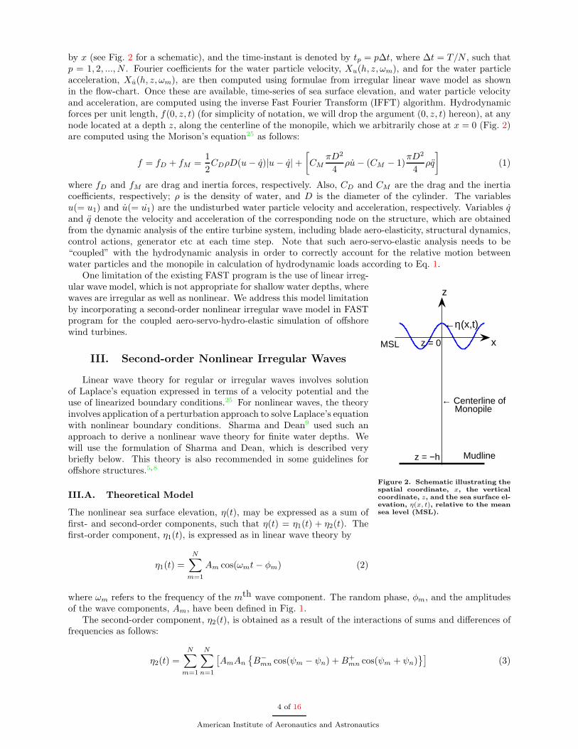
by x (see Fig. 2 for a schematic), and the time-instant is denoted by tp = p∆t, where ∆t = T/N , such thatp = 1, 2, ..., N . Fourier coefficients for the water particle velocity, Xu(h, z, ωm), and for the water particleacceleration, Xu(h, z, ωm), are then computed using formulae from irregular linear wave model as shownin the flow-chart. Once these are available, time-series of sea surface elevation, and water particle velocityand acceleration, are computed using the inverse Fast Fourier Transform (IFFT) algorithm. Hydrodynamicforces per unit length, f(0, z, t) (for simplicity of notation, we will drop the argument (0, z, t) hereon), at anynode located at a depth z, along the centerline of the monopile, which we arbitrarily chose at x = 0 (Fig. 2)are computed using the Morison’s equation25 as follows:

f = fD + fM =1

2CDρD(u− q)|u− q|+

[

CM

πD2

4ρu− (CM − 1)

πD2

4ρq

]

(1)

where fD and fM are drag and inertia forces, respectively. Also, CD and CM are the drag and the inertiacoefficients, respectively; ρ is the density of water, and D is the diameter of the cylinder. The variablesu(= u1) and u(= u1) are the undisturbed water particle velocity and acceleration, respectively. Variables qand q denote the velocity and acceleration of the corresponding node on the structure, which are obtainedfrom the dynamic analysis of the entire turbine system, including blade aero-elasticity, structural dynamics,control actions, generator etc at each time step. Note that such aero-servo-elastic analysis needs to be“coupled” with the hydrodynamic analysis in order to correctly account for the relative motion betweenwater particles and the monopile in calculation of hydrodynamic loads according to Eq. 1.

x

z

←η(x,t)

Mudline

MSL

← Centerline ofMonopile

z = −h

z = 0

Figure 2. Schematic illustrating thespatial coordinate, x, the verticalcoordinate, z, and the sea surface el-evation, η(x, t), relative to the meansea level (MSL).

One limitation of the existing FAST program is the use of linear irreg-ular wave model, which is not appropriate for shallow water depths, wherewaves are irregular as well as nonlinear. We address this model limitationby incorporating a second-order nonlinear irregular wave model in FASTprogram for the coupled aero-servo-hydro-elastic simulation of offshorewind turbines.

III. Second-order Nonlinear Irregular Waves

Linear wave theory for regular or irregular waves involves solutionof Laplace’s equation expressed in terms of a velocity potential and theuse of linearized boundary conditions.25 For nonlinear waves, the theoryinvolves application of a perturbation approach to solve Laplace’s equationwith nonlinear boundary conditions. Sharma and Dean9 used such anapproach to derive a nonlinear wave theory for finite water depths. Wewill use the formulation of Sharma and Dean, which is described verybriefly below. This theory is also recommended in some guidelines foroffshore structures.5, 8

III.A. Theoretical Model

The nonlinear sea surface elevation, η(t), may be expressed as a sum offirst- and second-order components, such that η(t) = η1(t) + η2(t). Thefirst-order component, η1(t), is expressed as in linear wave theory by

η1(t) =

N∑

m=1

Am cos(ωmt− φm) (2)

where ωm refers to the frequency of the mth wave component. The random phase, φm, and the amplitudesof the wave components, Am, have been defined in Fig. 1.

The second-order component, η2(t), is obtained as a result of the interactions of sums and differences offrequencies as follows:

η2(t) =

N∑

m=1

N∑

n=1

[AmAn

{B−

mn cos(ψm − ψn) +B+mn cos(ψm + ψn)

}](3)

4 of 16

American Institute of Aeronautics and Astronautics

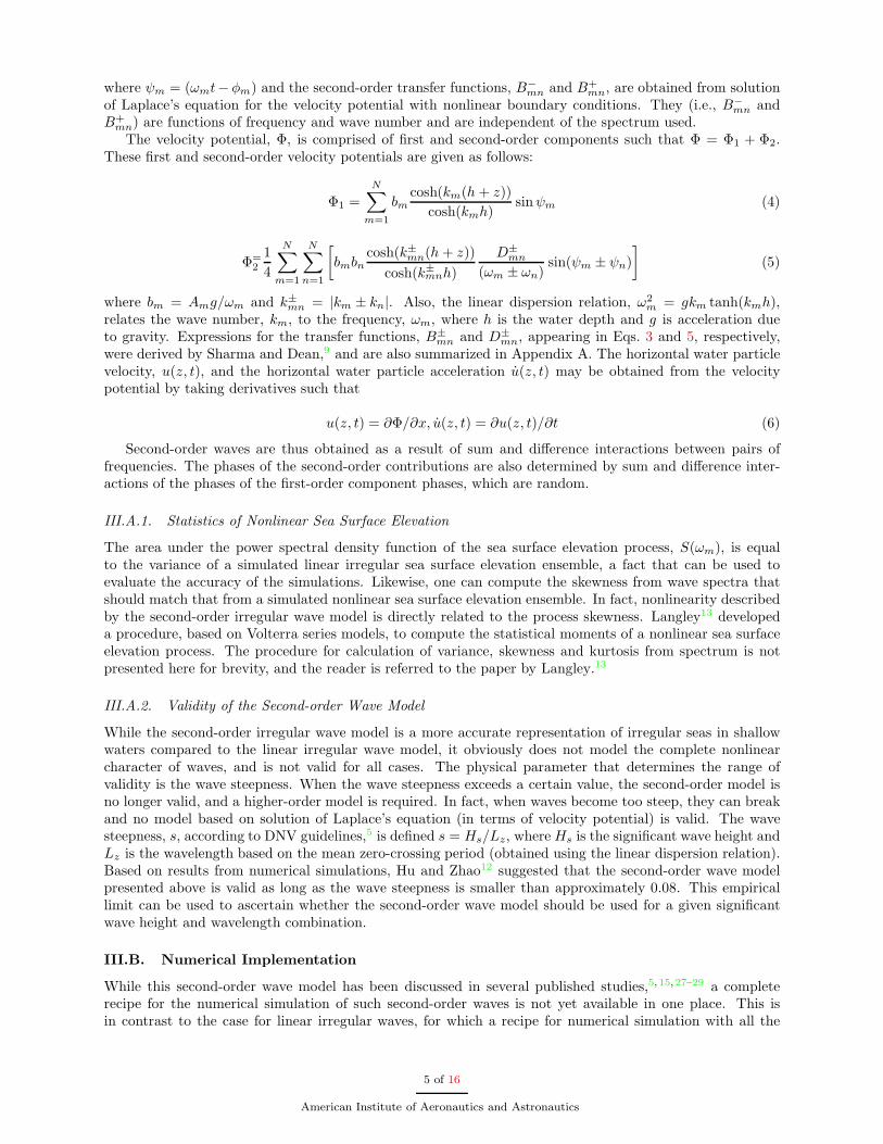
where ψm = (ωmt−φm) and the second-order transfer functions, B−mn and B+

mn, are obtained from solutionof Laplace’s equation for the velocity potential with nonlinear boundary conditions. They (i.e., B−

mn andB+

mn) are functions of frequency and wave number and are independent of the spectrum used.The velocity potential, Φ, is comprised of first and second-order components such that Φ = Φ1 + Φ2.

These first and second-order velocity potentials are given as follows:

Φ1 =

N∑

m=1

bmcosh(km(h+ z))

cosh(kmh)sinψm (4)

Φ=2

1

4

N∑

m=1

N∑

n=1

[

bmbncosh(k±mn(h+ z))

cosh(k±mnh)

D±mn

(ωm ± ωn)sin(ψm ± ψn)

]

(5)

where bm = Amg/ωm and k±mn = |km ± kn|. Also, the linear dispersion relation, ω2m = gkm tanh(kmh),

relates the wave number, km, to the frequency, ωm, where h is the water depth and g is acceleration dueto gravity. Expressions for the transfer functions, B±

mn and D±mn, appearing in Eqs. 3 and 5, respectively,

were derived by Sharma and Dean,9 and are also summarized in Appendix A. The horizontal water particlevelocity, u(z, t), and the horizontal water particle acceleration u(z, t) may be obtained from the velocitypotential by taking derivatives such that

u(z, t) = ∂Φ/∂x, u(z, t) = ∂u(z, t)/∂t (6)

Second-order waves are thus obtained as a result of sum and difference interactions between pairs offrequencies. The phases of the second-order contributions are also determined by sum and difference inter-actions of the phases of the first-order component phases, which are random.

III.A.1. Statistics of Nonlinear Sea Surface Elevation

The area under the power spectral density function of the sea surface elevation process, S(ωm), is equalto the variance of a simulated linear irregular sea surface elevation ensemble, a fact that can be used toevaluate the accuracy of the simulations. Likewise, one can compute the skewness from wave spectra thatshould match that from a simulated nonlinear sea surface elevation ensemble. In fact, nonlinearity describedby the second-order irregular wave model is directly related to the process skewness. Langley13 developeda procedure, based on Volterra series models, to compute the statistical moments of a nonlinear sea surfaceelevation process. The procedure for calculation of variance, skewness and kurtosis from spectrum is notpresented here for brevity, and the reader is referred to the paper by Langley.13

III.A.2. Validity of the Second-order Wave Model

While the second-order irregular wave model is a more accurate representation of irregular seas in shallowwaters compared to the linear irregular wave model, it obviously does not model the complete nonlinearcharacter of waves, and is not valid for all cases. The physical parameter that determines the range ofvalidity is the wave steepness. When the wave steepness exceeds a certain value, the second-order model isno longer valid, and a higher-order model is required. In fact, when waves become too steep, they can breakand no model based on solution of Laplace’s equation (in terms of velocity potential) is valid. The wavesteepness, s, according to DNV guidelines,5 is defined s = Hs/Lz, whereHs is the significant wave height andLz is the wavelength based on the mean zero-crossing period (obtained using the linear dispersion relation).Based on results from numerical simulations, Hu and Zhao12 suggested that the second-order wave modelpresented above is valid as long as the wave steepness is smaller than approximately 0.08. This empiricallimit can be used to ascertain whether the second-order wave model should be used for a given significantwave height and wavelength combination.

III.B. Numerical Implementation

While this second-order wave model has been discussed in several published studies,5, 15, 27–29 a completerecipe for the numerical simulation of such second-order waves is not yet available in one place. This isin contrast to the case for linear irregular waves, for which a recipe for numerical simulation with all the

5 of 16

American Institute of Aeronautics and Astronautics

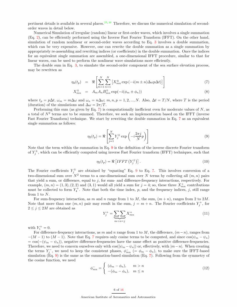
pertinent details is available in several places.25, 30 Therefore, we discuss the numerical simulation of second-order waves in detail below.

Numerical Simulation of irregular (random) linear or first-order waves, which involves a single summation(Eq. 2), can be efficiently performed using the Inverse Fast Fourier Transform (IFFT). On the other hand,simulation of random nonlinear or second-order waves according to Eq. 3 involves a double summation,which can be very expensive. However, one can rewrite the double summation as a single summation byappropriately re-assembling and rewriting indices (or coefficients) in the double summation. Once the indicesfor an equivalent single summation are assembled, a one-dimensional IFFT procedure, similar to that forlinear waves, can be used to perform the nonlinear wave simulations more efficiently.

The double sum in Eq. 3, to simulate the second-order component of the sea surface elevation process,may be rewritten as

η2(tp) = ℜ[

N∑

m=1

N∑

n=1

[X±

mn exp (−i(m± n)∆ωp∆t)]

]

(7)

X±mn = AmAnB

±mn exp(−i(φm ± φn)) (8)

where tp = p∆t, ωm = m∆ω and ωn = n∆ω; m,n, p = 1, 2, ..., N . Also, ∆t = T/N , where T is the period(duration) of the simulations and ∆ω = 2π/T .

Performing this sum (as given by Eq. 7) is computationally inefficient even for moderate values of N , asa total of N2 terms are to be summed. Therefore, we seek an implementation based on the IFFT (inverseFast Fourier Transform) technique. We start by rewriting the double summation in Eq. 7 as an equivalentsingle summation as follows:

η2(tp) = ℜ

N∑

j=1

Y ±j exp

(

−i2πjN

p

)

(9)

Note that the term within the summation in Eq. 9 is the definition of the inverse discrete Fourier transformof Y ±

j , which can be efficiently computed using inverse Fast Fourier transform (IFFT) techniques, such that

η2(tp) = ℜ[IFFT

(Y ±j

)]. (10)

The Fourier coefficients Y ±j are obtained by “equating” Eq. 9 to Eq. 7. This involves conversion of a

two-dimensional sum over N2 terms to a one-dimensional sum over N terms by collecting all (m,n) pairsthat yield a sum, or difference, equal to j, for sum- and difference-frequency interactions, respectively. Forexample, (m,n) = (1, 3), (2, 2) and (3, 1) would all yield a sum for j = 4; so, these three X+

mn contributionsmust be collected to form Y +

4 . Note that both the time index, p, and the frequency indices, j, still rangefrom 1 to N .

For sum-frequency interaction, as m and n range from 1 to M , the sum, (m+ n), ranges from 2 to 2M .Note that more than one (m,n) pair may result in the sum, j = m + n. The Fourier coefficients Y +

j , for2 ≤ j ≤ 2M are obtained as

Y +j =

∑∑

︸ ︷︷ ︸

m+n=j

X+mn (11)

with Y +1 = 0.

For difference-frequency interactions, as m and n range from 1 toM , the difference, (m−n), ranges from−(M − 1) to (M − 1). Note that Eq. 7 requires only cosine terms to be computed, and since cos(ψm − ψn)= cos(−(ψm − ψn)), negative difference-frequencies have the same effect as positive difference-frequencies.Therefore, we need to concern ourselves only with cos(|ψm−ψn|) or, effectively, with |m−n|. When creatingthe terms Y −

j , we need to keep the consistent phases, φ−mn (= φm − φn), to make sure the IFFT-basedsimulation (Eq. 9) is the same as the summation-based simulation (Eq. 7). Following from the symmetry ofthe cosine function, we need

φ−mn =

{

(φm − φn), m > n

−(φm − φn), m ≤ n(12)

6 of 16

American Institute of Aeronautics and Astronautics

The Fourier coefficients Y −j for 1 ≤ j ≤ (M − 1) are obtained as

Y −j =

∑∑

︸ ︷︷ ︸

|m−n|=j

X−mn (13)

with Y −j = 0 for j ≥M .

Using the procedure described above, we can obtain the coefficients, Y ±j , for Eq. 9 from Eqs. 11 and 13,

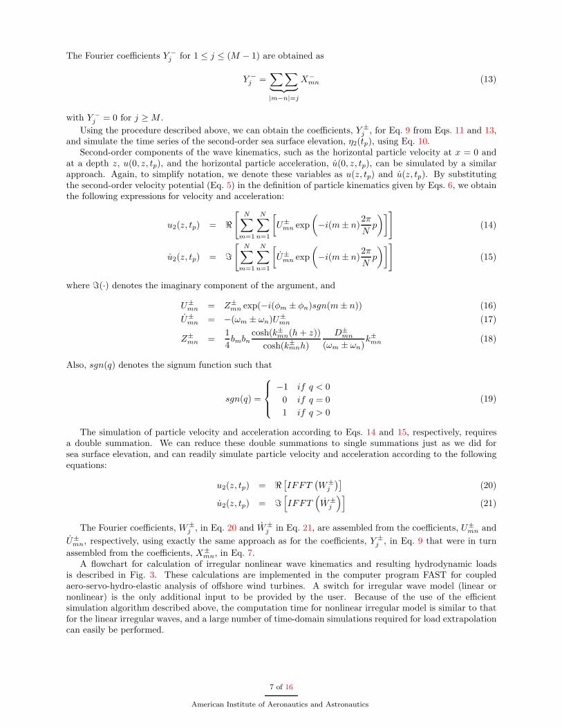
and simulate the time series of the second-order sea surface elevation, η2(tp), using Eq. 10.Second-order components of the wave kinematics, such as the horizontal particle velocity at x = 0 and

at a depth z, u(0, z, tp), and the horizontal particle acceleration, u(0, z, tp), can be simulated by a similarapproach. Again, to simplify notation, we denote these variables as u(z, tp) and u(z, tp). By substitutingthe second-order velocity potential (Eq. 5) in the definition of particle kinematics given by Eqs. 6, we obtainthe following expressions for velocity and acceleration:

u2(z, tp) = ℜ[

N∑

m=1

N∑

n=1

[

U±mn exp

(

−i(m± n)2π

Np

)]]

(14)

u2(z, tp) = ℑ[

N∑

m=1

N∑

n=1

[

U±mn exp

(

−i(m± n)2π

Np

)]]

(15)

where ℑ(·) denotes the imaginary component of the argument, and

U±mn = Z±

mn exp(−i(φm ± φn)sgn(m± n)) (16)

U±mn = −(ωm ± ωn)U

±mn (17)

Z±mn =

1

4bmbn

cosh(k±mn(h+ z))

cosh(k±mnh)

D±mn

(ωm ± ωn)k±mn (18)

Also, sgn(q) denotes the signum function such that

sgn(q) =

−1 if q < 0

0 if q = 0

1 if q > 0

(19)

The simulation of particle velocity and acceleration according to Eqs. 14 and 15, respectively, requiresa double summation. We can reduce these double summations to single summations just as we did forsea surface elevation, and can readily simulate particle velocity and acceleration according to the followingequations:

u2(z, tp) = ℜ[IFFT

(W±

j

)](20)

u2(z, tp) = ℑ[

IFFT(

W±j

)]

(21)

The Fourier coefficients, W±j , in Eq. 20 and W±

j in Eq. 21, are assembled from the coefficients, U±mn and

U±mn, respectively, using exactly the same approach as for the coefficients, Y ±

j , in Eq. 9 that were in turn

assembled from the coefficients, X±mn, in Eq. 7.

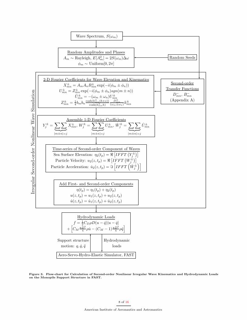
A flowchart for calculation of irregular nonlinear wave kinematics and resulting hydrodynamic loadsis described in Fig. 3. These calculations are implemented in the computer program FAST for coupledaero-servo-hydro-elastic analysis of offshore wind turbines. A switch for irregular wave model (linear ornonlinear) is the only additional input to be provided by the user. Because of the use of the efficientsimulation algorithm described above, the computation time for nonlinear irregular model is similar to thatfor the linear irregular waves, and a large number of time-domain simulations required for load extrapolationcan easily be performed.

7 of 16

American Institute of Aeronautics and Astronautics

Wave Spectrum, S(ωm)

Random Amplitudes and Phases

Am ∼ Rayleigh, E[A2m] = 2S(ωm)∆ω

φm ∼ Uniform[0, 2π]

Random Seeds

2-D Fourier Coefficients for Wave Elevation and Kinematics

X±mn = AmAnB

±mn exp(−i(φm ± φn))

U±mn = Z±

mn exp(−i(φm ± φn)sgn(m± n))

U±mn = −(ωm ± ωn)U

±mn

Z±mn = 1

4bmbncosh(k±

mn(h+z))

cosh(k±mnh)

D±mn

(ωm±ωn)k±mn

Second-order

Transfer Functions

D−mn, B

−mn

(Appendix A)

Assemble 1-D Fourier Coefficients

Y ±j =

∑∑

︸ ︷︷ ︸

|m±n|=j

X±mn, W

±j =

∑∑

︸ ︷︷ ︸

|m±n|=j

U±mn, W

±j =

∑∑

︸ ︷︷ ︸

|m±n|=j

U±mn

Time-series of Second-order Component of Waves

Sea Surface Elevation: η2(tp) = ℜ[IFFT

(Y ±j

)]

Particle Velocity: u2(z, tp) = ℜ[IFFT

(W±

j

)]

Particle Acceleration: u2(z, tp) = ℑ[

IFFT(

W±j

)]

Add First- and Second-order Components

η(tp) = η1(tp) + η2(tp)

u(z, tp) = u1(z, tp) + u2(z, tp)

u(z, tp) = u1(z, tp) + u2(z, tp)

Hydrodynamic Loads

f = 12CDρD(u− q)|u− q|

+[

CMπD2

4 ρu− (CM − 1)πD2

4 ρq]

Support structure

motion: q, q, q

Hydrodynamic

loads

Aero-Servo-Hydro-Elastic Simulator, FAST

IrregularSecond-order

NonlinearWaveSim

ulation

Figure 3. Flow-chart for Calculation of Second-order Nonlinear Irregular Wave Kinematics and Hydrodynamic Loadson the Monopile Support Structure in FAST.

8 of 16

American Institute of Aeronautics and Astronautics

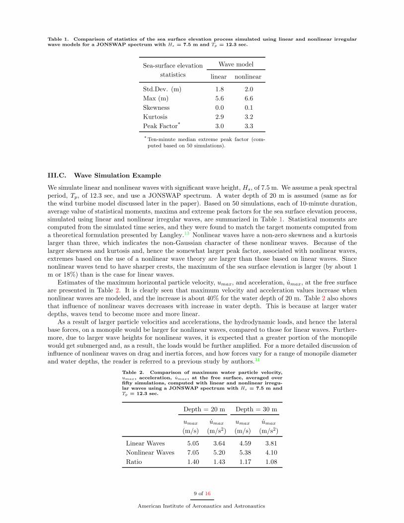
Table 1. Comparison of statistics of the sea surface elevation process simulated using linear and nonlinear irregularwave models for a JONSWAP spectrum with Hs = 7.5 m and Tp = 12.3 sec.

Sea-surface elevation Wave model

statistics linear nonlinear

Std.Dev. (m) 1.8 2.0

Max (m) 5.6 6.6

Skewness 0.0 0.1

Kurtosis 2.9 3.2

Peak Factor* 3.0 3.3

*Ten-minute median extreme peak factor (com-puted based on 50 simulations).

III.C. Wave Simulation Example

We simulate linear and nonlinear waves with significant wave height, Hs, of 7.5 m. We assume a peak spectralperiod, Tp, of 12.3 sec, and use a JONSWAP spectrum. A water depth of 20 m is assumed (same as forthe wind turbine model discussed later in the paper). Based on 50 simulations, each of 10-minute duration,average value of statistical moments, maxima and extreme peak factors for the sea surface elevation process,simulated using linear and nonlinear irregular waves, are summarized in Table 1. Statistical moments arecomputed from the simulated time series, and they were found to match the target moments computed froma theoretical formulation presented by Langley.13 Nonlinear waves have a non-zero skewness and a kurtosislarger than three, which indicates the non-Gaussian character of these nonlinear waves. Because of thelarger skewness and kurtosis and, hence the somewhat larger peak factor, associated with nonlinear waves,extremes based on the use of a nonlinear wave theory are larger than those based on linear waves. Sincenonlinear waves tend to have sharper crests, the maximum of the sea surface elevation is larger (by about 1m or 18%) than is the case for linear waves.

Estimates of the maximum horizontal particle velocity, umax, and acceleration, umax, at the free surfaceare presented in Table 2. It is clearly seen that maximum velocity and acceleration values increase whennonlinear waves are modeled, and the increase is about 40% for the water depth of 20 m. Table 2 also showsthat influence of nonlinear waves decreases with increase in water depth. This is because at larger waterdepths, waves tend to become more and more linear.

As a result of larger particle velocities and accelerations, the hydrodynamic loads, and hence the lateralbase forces, on a monopile would be larger for nonlinear waves, compared to those for linear waves. Further-more, due to larger wave heights for nonlinear waves, it is expected that a greater portion of the monopilewould get submerged and, as a result, the loads would be further amplified. For a more detailed discussion ofinfluence of nonlinear waves on drag and inertia forces, and how forces vary for a range of monopile diameterand water depths, the reader is referred to a previous study by authors.31

Table 2. Comparison of maximum water particle velocity,umax, acceleration, umax, at the free surface, averaged overfifty simulations, computed with linear and nonlinear irregu-lar waves using a JONSWAP spectrum with Hs = 7.5 m andTp = 12.3 sec.

Depth = 20 m Depth = 30 m

umax umax umax umax

(m/s) (m/s2) (m/s) (m/s2)

Linear Waves 5.05 3.64 4.59 3.81

Nonlinear Waves 7.05 5.20 5.38 4.10

Ratio 1.40 1.43 1.17 1.08

9 of 16

American Institute of Aeronautics and Astronautics

IV. Effect of Wave Model on Turbine Loads

We now investigate how the alternative wave models discussed above affect the response of an offshorewind turbine. We focus on the fore-aft tower bending moment and the shear force at mudline, as these aredirectly effected by waves. Loads on the turbine rotor, on the other hand, are not affected as much by wavesas by wind. In the following, we first discuss the turbine model used, and then compare time-series andstatistics of the fore-aft tower bending moment resulting from linear and nonlinear wave models. We finallycompute loads for a return period of 20 years in order to assess influence of the alternative wave models onlong-term loads.

IV.A. Turbine Model

A 5MW wind turbine model developed at NREL23 closely representing utility-scale offshore wind turbinesbeing manufactured today is considered here. The turbine is a variable-speed, collective pitch-controlledmachine with a maximum rotor speed of 12.1 rpm; its rated wind speed is 11.5 m/s. It is assumed to havea hub height of 90 meters above the mean sea level, and a rotor diameter of 126 meters. It is assumed tobe sited in 20 meters of water; it has a monopile support structure of 6 m diameter, which is assumed to berigidly connected to the seafloor. The turbine is assumed to be installed at an IEC Class I-B wind regimesite.4 A Kaimal power spectrum and an exponential coherence spectrum are employed to describe the inflowturbulence random field over the rotor plane, which is simulated using the computer program, TurbSim.32

For the hydrodynamic loading on the support structure, irregular long-crested waves are simulated usinga JONSWAP spectrum.33 This same wave spectrum is used for simulating linear and nonlinear irregularwaves. Hydrodynamic loads are computed using Morison’s equation (Eq. 1); Wheeler stretching5 is used torepresent water particle kinematics and hydrodynamic loads up to the changing instantaneous sea surface.

IV.B. Turbine Response

We consider environmental conditions involving a significant wave height of 7.5 m with a mean wind speedof 18 m/s. This combination of V and Hs governs long-term fore-aft tower bending moment at the mudlinefor a return period of 20 years; we will discuss long-term loads later in the paper, and for now, we discusshow linear and nonlinear irregular waves influence the turbine response.

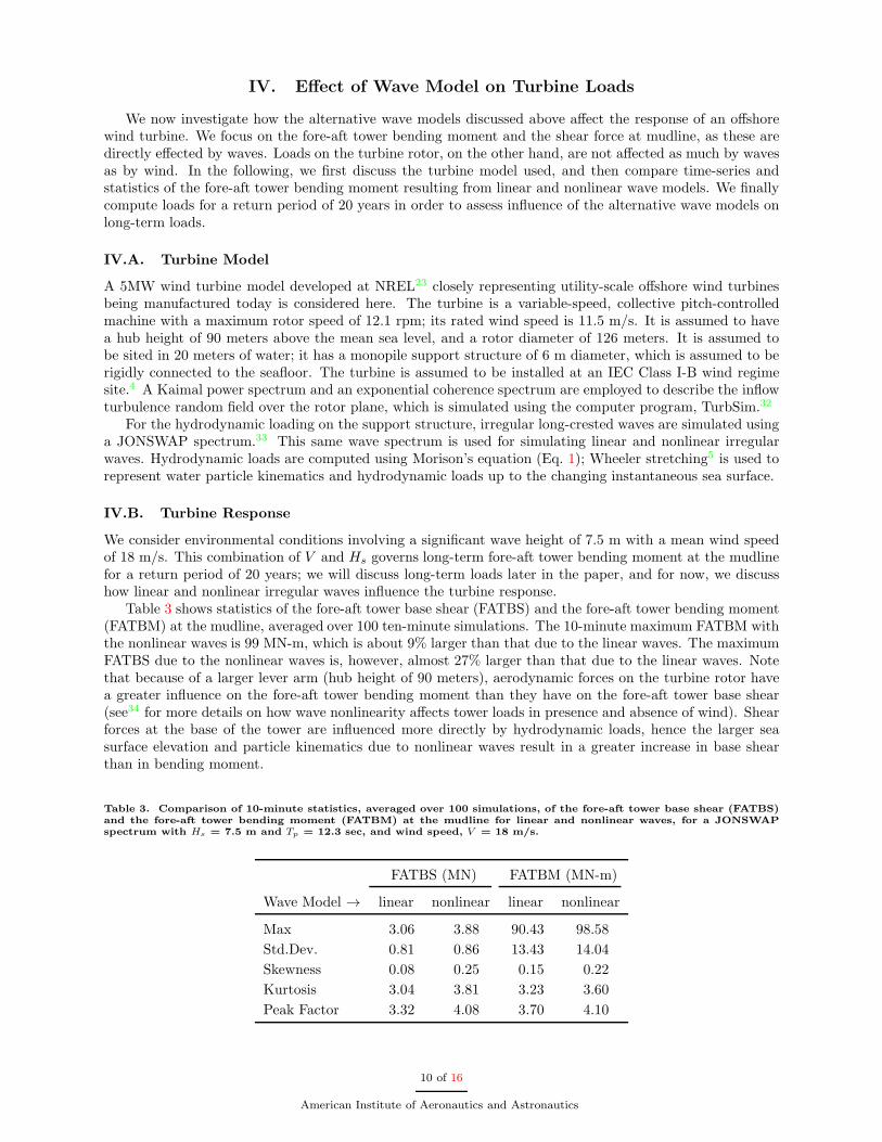
Table 3 shows statistics of the fore-aft tower base shear (FATBS) and the fore-aft tower bending moment(FATBM) at the mudline, averaged over 100 ten-minute simulations. The 10-minute maximum FATBM withthe nonlinear waves is 99 MN-m, which is about 9% larger than that due to the linear waves. The maximumFATBS due to the nonlinear waves is, however, almost 27% larger than that due to the linear waves. Notethat because of a larger lever arm (hub height of 90 meters), aerodynamic forces on the turbine rotor havea greater influence on the fore-aft tower bending moment than they have on the fore-aft tower base shear(see34 for more details on how wave nonlinearity affects tower loads in presence and absence of wind). Shearforces at the base of the tower are influenced more directly by hydrodynamic loads, hence the larger seasurface elevation and particle kinematics due to nonlinear waves result in a greater increase in base shearthan in bending moment.

Table 3. Comparison of 10-minute statistics, averaged over 100 simulations, of the fore-aft tower base shear (FATBS)and the fore-aft tower bending moment (FATBM) at the mudline for linear and nonlinear waves, for a JONSWAPspectrum with Hs = 7.5 m and Tp = 12.3 sec, and wind speed, V = 18 m/s.

FATBS (MN) FATBM (MN-m)

Wave Model → linear nonlinear linear nonlinear

Max 3.06 3.88 90.43 98.58

Std.Dev. 0.81 0.86 13.43 14.04

Skewness 0.08 0.25 0.15 0.22

Kurtosis 3.04 3.81 3.23 3.60

Peak Factor 3.32 4.08 3.70 4.10

10 of 16

American Institute of Aeronautics and Astronautics

300 320 340 360 380 400 420 440 460 480 50010

20

30Wind Speed (m/s)

300 320 340 360 380 400 420 440 460 480 500−5

0

5

Wave Elevation (m)

Linear Nonlinear

300 320 340 360 380 400 420 440 460 480 500−4−2

024

Fore−aft Tower Base Shear (MN−m)

300 320 340 360 380 400 420 440 460 480 5000

50100

Fore−aft Tower Base Momemt (MN−m)

time (sec)

(a) A 200-second segment of time series

0.1 0.2 0.3 0.410

−1

100

101

102

103 Wind Speed

Frequency (Hz)

PS

D [(

m/s

)2 /Hz]

0.1 0.2 0.3 0.40

20

40

60

80

100Wave Elevation

Frequency (Hz)

PS

D [(

m)2 /H

z]

LinearNonlinear

0.1 0.2 0.3 0.40

5

10

15FATBS

Frequency (Hz)

PS

D [(

MN

)2 /Hz]

0.1 0.2 0.3 0.40

500

1000

1500

2000

2500FATBM

Frequency (Hz)

PS

D [(

MN

−m

)2 /Hz]

(b) Power spectral densities (PSD)

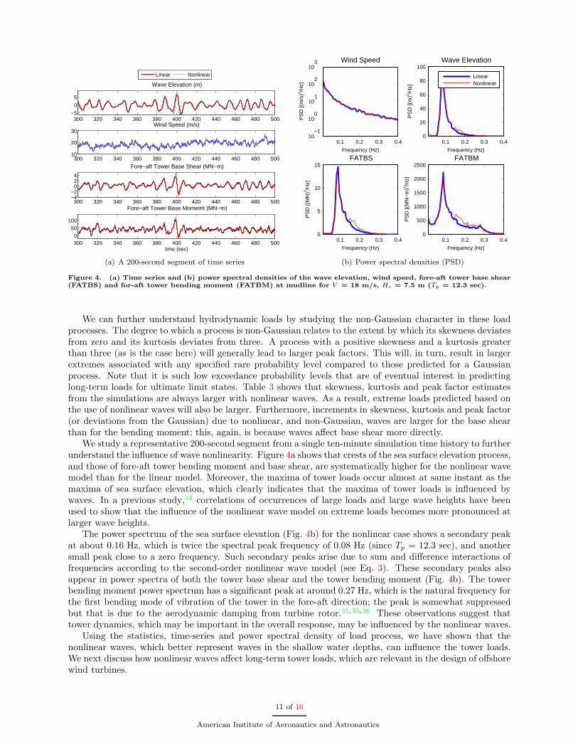
Figure 4. (a) Time series and (b) power spectral densities of the wave elevation, wind speed, fore-aft tower base shear(FATBS) and for-aft tower bending moment (FATBM) at mudline for V = 18 m/s, Hs = 7.5 m (Tp = 12.3 sec).

We can further understand hydrodynamic loads by studying the non-Gaussian character in these loadprocesses. The degree to which a process is non-Gaussian relates to the extent by which its skewness deviatesfrom zero and its kurtosis deviates from three. A process with a positive skewness and a kurtosis greaterthan three (as is the case here) will generally lead to larger peak factors. This will, in turn, result in largerextremes associated with any specified rare probability level compared to those predicted for a Gaussianprocess. Note that it is such low exceedance probability levels that are of eventual interest in predictinglong-term loads for ultimate limit states. Table 3 shows that skewness, kurtosis and peak factor estimatesfrom the simulations are always larger with nonlinear waves. As a result, extreme loads predicted based onthe use of nonlinear waves will also be larger. Furthermore, increments in skewness, kurtosis and peak factor(or deviations from the Gaussian) due to nonlinear, and non-Gaussian, waves are larger for the base shearthan for the bending moment; this, again, is because waves affect base shear more directly.

We study a representative 200-second segment from a single ten-minute simulation time history to furtherunderstand the influence of wave nonlinearity. Figure 4a shows that crests of the sea surface elevation process,and those of fore-aft tower bending moment and base shear, are systematically higher for the nonlinear wavemodel than for the linear model. Moreover, the maxima of tower loads occur almost at same instant as themaxima of sea surface elevation, which clearly indicates that the maxima of tower loads is influenced bywaves. In a previous study,34 correlations of occurrences of large loads and large wave heights have beenused to show that the influence of the nonlinear wave model on extreme loads becomes more pronounced atlarger wave heights.

The power spectrum of the sea surface elevation (Fig. 4b) for the nonlinear case shows a secondary peakat about 0.16 Hz, which is twice the spectral peak frequency of 0.08 Hz (since Tp = 12.3 sec), and anothersmall peak close to a zero frequency. Such secondary peaks arise due to sum and difference interactions offrequencies according to the second-order nonlinear wave model (see Eq. 3). These secondary peaks alsoappear in power spectra of both the tower base shear and the tower bending moment (Fig. 4b). The towerbending moment power spectrum has a significant peak at around 0.27 Hz, which is the natural frequency forthe first bending mode of vibration of the tower in the fore-aft direction; the peak is somewhat suppressedbut that is due to the aerodynamic damping from turbine rotor.31, 35, 36 These observations suggest thattower dynamics, which may be important in the overall response, may be influenced by the nonlinear waves.

Using the statistics, time-series and power spectral density of load process, we have shown that thenonlinear waves, which better represent waves in the shallow water depths, can influence the tower loads.We next discuss how nonlinear waves affect long-term tower loads, which are relevant in the design of offshorewind turbines.

11 of 16

American Institute of Aeronautics and Astronautics

50 100 150 200 25010

−6

10−4

10−2

100

Fore−aft Tower Bending Momemt (MN−m)

Exc

eeda

nce

Pro

babi

lity

in 1

0−m

inut

es

Linear wavesNonlinear waves

(a) V = 16 m/s, Hs = 5.5 m.

50 100 150 200 25010

−6

10−4

10−2

100

Fore−aft Tower Bending Momemt (MN−m)

Exc

eeda

nce

Pro

babi

lity

in 1

0−m

inut

es

Linear wavesNonlinear waves

(b) V = 18 m/s, Hs = 7.5 m.

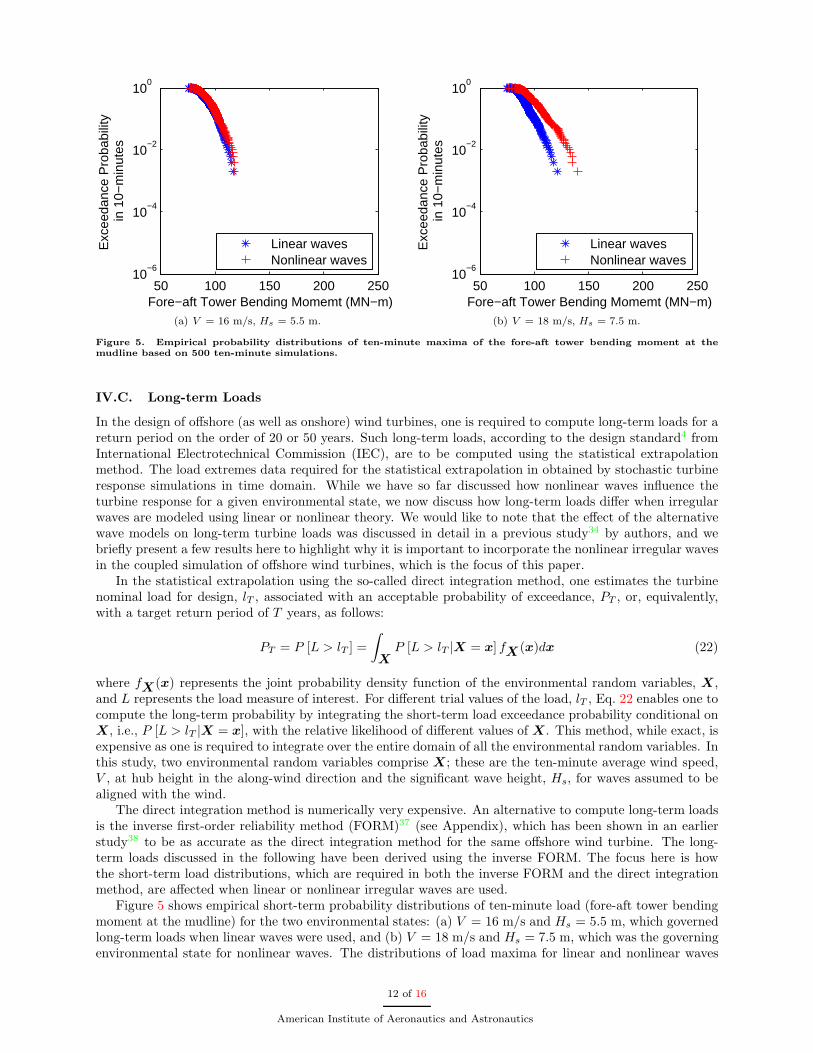
Figure 5. Empirical probability distributions of ten-minute maxima of the fore-aft tower bending moment at themudline based on 500 ten-minute simulations.

IV.C. Long-term Loads

In the design of offshore (as well as onshore) wind turbines, one is required to compute long-term loads for areturn period on the order of 20 or 50 years. Such long-term loads, according to the design standard4 fromInternational Electrotechnical Commission (IEC), are to be computed using the statistical extrapolationmethod. The load extremes data required for the statistical extrapolation in obtained by stochastic turbineresponse simulations in time domain. While we have so far discussed how nonlinear waves influence theturbine response for a given environmental state, we now discuss how long-term loads differ when irregularwaves are modeled using linear or nonlinear theory. We would like to note that the effect of the alternativewave models on long-term turbine loads was discussed in detail in a previous study34 by authors, and webriefly present a few results here to highlight why it is important to incorporate the nonlinear irregular wavesin the coupled simulation of offshore wind turbines, which is the focus of this paper.

In the statistical extrapolation using the so-called direct integration method, one estimates the turbinenominal load for design, lT , associated with an acceptable probability of exceedance, PT , or, equivalently,with a target return period of T years, as follows:

PT = P [L > lT ] =

∫

X

P [L > lT |X = x] fX (x)dx (22)

where fX(x) represents the joint probability density function of the environmental random variables, X,and L represents the load measure of interest. For different trial values of the load, lT , Eq. 22 enables one tocompute the long-term probability by integrating the short-term load exceedance probability conditional onX, i.e., P [L > lT |X = x], with the relative likelihood of different values of X. This method, while exact, isexpensive as one is required to integrate over the entire domain of all the environmental random variables. Inthis study, two environmental random variables comprise X; these are the ten-minute average wind speed,V , at hub height in the along-wind direction and the significant wave height, Hs, for waves assumed to bealigned with the wind.

The direct integration method is numerically very expensive. An alternative to compute long-term loadsis the inverse first-order reliability method (FORM)37 (see Appendix), which has been shown in an earlierstudy38 to be as accurate as the direct integration method for the same offshore wind turbine. The long-term loads discussed in the following have been derived using the inverse FORM. The focus here is howthe short-term load distributions, which are required in both the inverse FORM and the direct integrationmethod, are affected when linear or nonlinear irregular waves are used.

Figure 5 shows empirical short-term probability distributions of ten-minute load (fore-aft tower bendingmoment at the mudline) for the two environmental states: (a) V = 16 m/s and Hs = 5.5 m, which governedlong-term loads when linear waves were used, and (b) V = 18 m/s and Hs = 7.5 m, which was the governingenvironmental state for nonlinear waves. The distributions of load maxima for linear and nonlinear waves

12 of 16

American Institute of Aeronautics and Astronautics

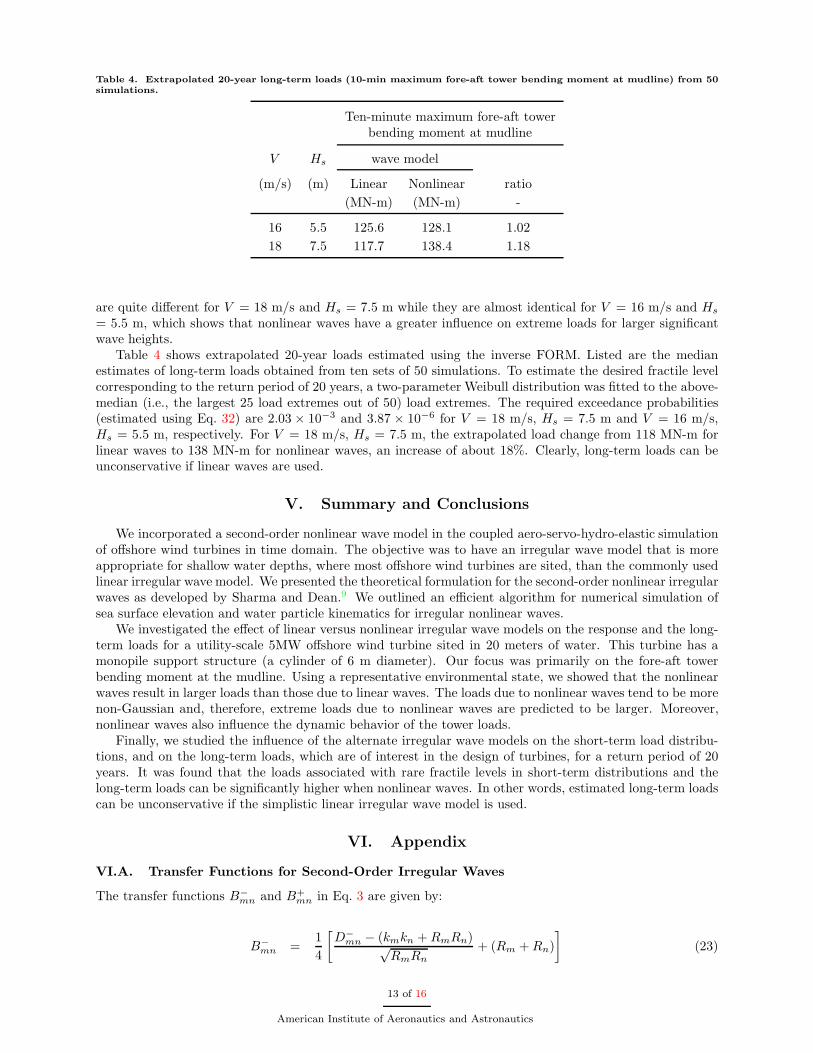
Table 4. Extrapolated 20-year long-term loads (10-min maximum fore-aft tower bending moment at mudline) from 50simulations.

Ten-minute maximum fore-aft towerbending moment at mudline

V Hs wave model

(m/s) (m) Linear Nonlinear ratio

(MN-m) (MN-m) -

16 5.5 125.6 128.1 1.02

18 7.5 117.7 138.4 1.18

are quite different for V = 18 m/s and Hs = 7.5 m while they are almost identical for V = 16 m/s and Hs

= 5.5 m, which shows that nonlinear waves have a greater influence on extreme loads for larger significantwave heights.

Table 4 shows extrapolated 20-year loads estimated using the inverse FORM. Listed are the medianestimates of long-term loads obtained from ten sets of 50 simulations. To estimate the desired fractile levelcorresponding to the return period of 20 years, a two-parameter Weibull distribution was fitted to the above-median (i.e., the largest 25 load extremes out of 50) load extremes. The required exceedance probabilities(estimated using Eq. 32) are 2.03 × 10−3 and 3.87 × 10−6 for V = 18 m/s, Hs = 7.5 m and V = 16 m/s,Hs = 5.5 m, respectively. For V = 18 m/s, Hs = 7.5 m, the extrapolated load change from 118 MN-m forlinear waves to 138 MN-m for nonlinear waves, an increase of about 18%. Clearly, long-term loads can beunconservative if linear waves are used.

V. Summary and Conclusions

We incorporated a second-order nonlinear wave model in the coupled aero-servo-hydro-elastic simulationof offshore wind turbines in time domain. The objective was to have an irregular wave model that is moreappropriate for shallow water depths, where most offshore wind turbines are sited, than the commonly usedlinear irregular wave model. We presented the theoretical formulation for the second-order nonlinear irregularwaves as developed by Sharma and Dean.9 We outlined an efficient algorithm for numerical simulation ofsea surface elevation and water particle kinematics for irregular nonlinear waves.

We investigated the effect of linear versus nonlinear irregular wave models on the response and the long-term loads for a utility-scale 5MW offshore wind turbine sited in 20 meters of water. This turbine has amonopile support structure (a cylinder of 6 m diameter). Our focus was primarily on the fore-aft towerbending moment at the mudline. Using a representative environmental state, we showed that the nonlinearwaves result in larger loads than those due to linear waves. The loads due to nonlinear waves tend to be morenon-Gaussian and, therefore, extreme loads due to nonlinear waves are predicted to be larger. Moreover,nonlinear waves also influence the dynamic behavior of the tower loads.

Finally, we studied the influence of the alternate irregular wave models on the short-term load distribu-tions, and on the long-term loads, which are of interest in the design of turbines, for a return period of 20years. It was found that the loads associated with rare fractile levels in short-term distributions and thelong-term loads can be significantly higher when nonlinear waves. In other words, estimated long-term loadscan be unconservative if the simplistic linear irregular wave model is used.

VI. Appendix

VI.A. Transfer Functions for Second-Order Irregular Waves

The transfer functions B−mn and B+

mn in Eq. 3 are given by:

B−mn =

1

4

[D−

mn − (kmkn +RmRn)√RmRn

+ (Rm +Rn)

]

(23)

13 of 16

American Institute of Aeronautics and Astronautics

B+mn =

1

4

[D+

mn − (kmkn −RmRn)√RmRn

+ (Rm +Rn)

]

(24)

where

D−mn =

(√Rm −

√Rn)

{√Rn(k

2m −R2

m)−√Rm(k2n −R2

n)}

(√Rm −

√Rn)2 − k−mn tanh(k

−mnh)

(25)

+2(√Rm −

√Rn)

2(kmkn +RmRn)

(√Rm −

√Rn)2 − k−mn tanh(k−mnh)

D+mn =

(√Rm +

√Rn)

{√Rn(k

2m −R2

m) +√Rm(k2n −R2

n)}

(√Rm +

√Rn)2 − k+mn tanh(k

+mnh)

(26)

+2(√Rm +

√Rn)

2(kmkn −RmRn)

(√Rm +

√Rn)2 − k+mn tanh(k+mnh)

In the above, k is the wave number which is related the frequency, ω, and the water depth, h, via thedispersion relation. Related parameters that are needed are given as follows:

ω2 = gk tanh(kh) (27)

Rm =ω2m

g(28)

k−mn = |km − kn| (29)

k+mn = km + kn (30)

where g refers to acceleration due to gravity.

VI.B. Inverse First-order Reliability Method

In the inverse FORM, for the present application, one considers a surface in a three-dimensional space,Y = (V,Hs, L), of physical random variables, on one side of which (i.e., the “failure” side), it is assumedthat L > lT . It is possible to mathematically transform this space to an independent standard normal spaceU = (U1, U2, U3). A sphere of radius, β, in the standard normal space is defined as follows:

u21 + u22 + u23 = β2 (31)

This sphere is such that all values of U within it occur with a probability greater than PT while all valuesoutside it occurs with a probability less than PT .

It is noted here that β is directly related to the target probability of load exceedance; namely, PT =Φ(−β), where Φ() represents the cumulative distribution function of a standard normal random variable.The transformation of the random variables involved from the physical space, Y , to the standard normalU space is carried out via the Rosenblatt transformation such that FV (v) = Φ(u1), FH|V (h) = Φ(u2), andFL|V,H(l) = Φ(u3), where F () denotes the cumulative distribution function in each case. A point on thesphere defined by Eq. 31 where the load attains its maximum value is the “design” point, and this loadrepresents the desired nominal T -year return period load, lT .

According to inverse FORM, we estimate the load for the fractile level, p3 = Φ(u3), for all possible(V,Hs) pairs, and largest of such load fractiles is the nominal load, lT . Based on Eq. 31, the fractile level,p3, corresponding to the target reliability index, β, is obtained as follows:

p3 = Φ

(√

β2 − [Φ−1 (FV (v))]2 −

[Φ−1

(FH|V (h)

)]2)

(32)

VII. Acknowledgments

The authors gratefully acknowledge assistance received with the 5MW offshore wind turbine baselinemodel used in the simulation studies from Dr. Jason Jonkman of the National Renewable Energy Laboratory.

14 of 16

American Institute of Aeronautics and Astronautics

The authors also wish to acknowledge the financial support provided by the National Science Foundation(CAREER Award No. CMMI-0449128 and Award No. CMMI-0727989) and by Sandia National Laboratories(Contract No. 743358). The first author also acknowledges Stress Engineering Services for providing financialsupport to attend the conference.

References

1Musial, W. and Butterfield, S., “Future for Offshore Wind Energy in the United States,” Tech. Rep. NREL/CP-500-36313,National Renewable Energy Laboratory, Golden, CO, 2004.

2European Wind Energy Association, Response to the European Commissions’s Green Paper: A European Strategy for

Sustainable, Competitive and Secure Energy, EWEA Position Paper , Brussels, Belgium, 2006.3European Wind Energy Association, Delivering Offshore Wind Power in Europe — Policy Recommendations for Large-

scale Deployment of Offshore Wind Power in Europe by 2020 , Brussels, Belgium, 2007.4IEC-61400-3, Wind Turbines - Part 3: Design Requirements for Offshore Wind Turbines, International Electrotechnical

Commission, TC88 WG3 Committee Draft, 2005.5DNV-RP-C205, Environmental Conditions and Environmental Loads, Recommended Practice, Det Norske Veritas, 2007.6Forristall, G. Z., “Nonlinear Wave Calculations for Engineering Applications,” Journal of Offshore Mechanics and Arctic

Engineering , Vol. 124, No. 1, 2002, pp. 28–33.7Jha, A. K., Nonlinear Stochastic Models for Ocean Wave Loads and Responses of Offshore Structures and Vessels, Ph.D.

Dissertation, Stanford University, 1997.8ITTC, “The Specialist Committee on Environmental Modeliing, Final Report and Recommendations to the 22nd ITTC,”

Tech. rep., International Towing Tank Conference, Seoul, 1999.9Sharma, J. N. and Dean, R. G., “Development and Evaluation of a Procedure for Simulating a Random Directional

Second-order Sea Surface and Associated Wave Forces,” Tech. Rep. Ocean Engineering Report No. 20, University of Delaware,Newark, DE, 1979.

10Longuet-Higgins, M., “Resonant Interactions between two Trains of Gravity Waves,” Journal of Fluid Mechanics, Vol. 12,No. 3, 1962, pp. 321–332.

11Hasselmann, K., “On the Non-linear Energy Transfer in a Gravity Wave Spectrum, Part 1, General Theory,” Journal of

Fluid Mechanics, Vol. 12, 1962, pp. 481–500.12Hu, S.-L. J. and Zhao, D., “Non-Gaussian Properties of Second-order Random Waves,” Journal of Engineering Mechan-

ics, Vol. 119, No. 2, 1993, pp. 344–364.13Langley, R., “A Statistical Analysis of Nonlinear Random Waves,” Ocean Engineering , Vol. 14, No. 5, 1987, pp. 389–407.14Longuet-Higgins, M., “The Propagation of Short Surface Waves on Longer Gravity Waves,” Journal of Fluid Mechanics,

Vol. 177, 1987, pp. 293–306.15Forristall, G. Z., “Wave Crest Distributions: Observations and Second-Order Theory,” Journal of Physical Oceanography ,

Vol. 30, No. 8, 2000, pp. 1931–1943.16Forristall, G. Z., “Irregular Wave Kinematics from a Kinematic Boundary Condition Fit (KBCF),” Applied Ocean Re-

search, Vol. 7, No. 4, 1985, pp. 202–212.17Tromans, P. S., Anaturk, A. R., and Hagemeijer, P., “A New Model for Kinematics of Large Ocean Waves — Application

as a Design Wave,” 1st International Offshore and Polar Engineering Conference, ISOPE1991 , Vol. 3, Edinburg, Scotland,1991.

18Taylor, P. H., Jonathan, P., and Harland, L. A., “Time-domain Simulation of Jack-up Dynamics with the Extremes ofa Gaussian Process,” 14th International Conference on Offshore Mechanics and Arctic Engineering, OMAE1995 , Volume 1A,pp. 313-319, Copenhagen, Denmark, 1995, pp. 313–319.

19Zhang, J., Chen, L., Ye, M., and Randall, R. E., “Hybrid Wave Model for Unidirectional Irregular Waves — Part I.Theory and Numerical Scheme,” Applied Ocean Research, Vol. 18, 1996, pp. 77–92.

20Nwogu, O., “Alternative form of Boussinesq Equations for Nearshore Wave Propagation,” Journal of Waterway, Port,

Coastal and Ocean Engineering , Vol. 119, No. 6, 1993, pp. 618–638.21Madsen, P. A., Bingham, H. B., and Liu, H., “A new Boussinesq method for Fully Nonlinear Waves from Shallow to

Deep Water,” Journal of Fluid Mechanics, Vol. 462, 2002, pp. 1–30.22Jonkman, J. M. and Buhl Jr., M. L., “FAST User’s Guide,” Tech. Rep. NREL/EL-500-38230, National Renewable Energy

Laboratory, Golden, CO, 2005.23Jonkman, J. M., Butterfield, S., Musial, W., and Scott, G., “Definition of a 5-MW Reference Wind Turbine for Offshore

System Development,” Tech. Rep. NREL/TP-500-38060, National Renewable Energy Laboratory, Golden, CO, 2007 (to bepublished).

24Burton, T., Sharpe, D., Jenkins, N., and Bossanyi, E., Wind Energy Handbook , John Wiley, Chichester, England, 2001.25Barltrop, N. D. P. and Adams, A. J., Dynamics of Fixed Marine Structures, Third Edition, Butterworth-Heinemann,

London, 1991.26Sarpkaya, T. and Issacson, M., Mechanics of Wave Forces on offshore Structures, Van Nostrand Reinhold, New York,

1981.27Sharma, J. N., Development and Evaluation of a Procedure for Simulating a Random Directional Second-order Sea

Surface and Associated Wave Forces, Ph.D. thesis, University of Delaware, Delaware, 1979.28Hudspeth, R. and Chen, M.-C., “Digital Simulation of Nonlinear Random Waves,” Journal of Waterway, Port, Coastal

and Ocean Division, ASCE , Vol. 105, No. WW1, 1979, pp. 67–85.

15 of 16

American Institute of Aeronautics and Astronautics

29Hu, S.-L. J., Nonlinear Random Water Wave, In Computational Stochastic Mechanics, A.H.-D. Chang and C.Y.Yang,eds., Computational Mechanics Publication, Southampton, UK, 519-544, 1993.

30Shinozuka, M. and Deodatis, G., “Simulation of Stochastic Processes by Spectral Representation,” Applied Mechanics

Reviews, Vol. 44, No. 4, 1991, pp. 191–203.31Agarwal, P. and Manuel, L., “Wave Models for Offshore Wind Turbines,” ASME Wind Energy Symposium, AIAA, Reno,

NV, 2008.32Jonkman, B. J. and Buhl Jr., M. L., “TurbSim User’s Guide,” Tech. Rep. NREL/TP-500-41136, National Renewable

Energy Laboratory, Golden, CO, 2007.33DNV-OS-J101, Design of Offshore Wind Turbine Structures, Offshore Standard , Det Norske Veritas, 2007.34Agarwal, P. and Manuel, L., “Modeling Nonlinear Irregular Waves in Reliability Studies for Offshore Wind Turbines,”

28th International Conference on Offshore Mechanics and Arctic Engineering, OMAE2009 , Paper no. 80149, Honolulu, Hawai,2009.

35Jonkman, J., Butterfield, S. P., Passon, P., Larsen, T., Camp, T., Nichols, J., Azcona, J., and Martinez, A., “OffshoreCode Comparison Collaboration within IEA Wind Annex XXIII: Phase II Results Regarding Monopile Foundation Modeling,”Tech. Rep. NREL/CP-500-42471, National Renewable Energy Laboratory, Golden, CO, 2008.

36Tempel, J. and Molenaar, D.-P., “Wind Turbine Structural Dynamics - A Review of the Principles for Modern PowerGeneration, Onshore and Offshore,” Wind Engineering , Vol. 26, No. 4, 2002, pp. 211–220.

37Winterstein, S. R., Ude, T. C., Cornell, C. A., Bjerager, P., and Haver, S., “Environmental Contours for ExtremeResponse: Inverse FORM with Omission Factors,” Proceedings, ICOSSAR-93 , Innsbruck, Austria, 1993.

38Agarwal, P. and Manuel, L., “Simulation of Offshore Wind Turbine Response for Extreme Limit States,” 26th Interna-

tional Conference on Offshore Mechanics and Arctic Engineering, OMAE2007 , Paper no. 29326, San Diego, CA, 2007.

16 of 16

American Institute of Aeronautics and Astronautics