This is a repository copy of Incompressible SPH simulation of open channel flow over smooth bed.

White Rose Research Online URL for this paper:http://eprints.whiterose.ac.uk/90419/

Version: Accepted Version

Article:

Tan, S.K., Cheng, N.S., Xie, Y. et al. (1 more author) (2015) Incompressible SPH simulation of open channel flow over smooth bed. Journal of Hydro-Environment Research, 9 (3). 340 - 353. ISSN 1570-6443

https://doi.org/10.1016/j.jher.2014.12.006

eprints@whiterose.ac.ukhttps://eprints.whiterose.ac.uk/

Reuse

Unless indicated otherwise, fulltext items are protected by copyright with all rights reserved. The copyright exception in section 29 of the Copyright, Designs and Patents Act 1988 allows the making of a single copy solely for the purpose of non-commercial research or private study within the limits of fair dealing. The publisher or other rights-holder may allow further reproduction and re-use of this version - refer to the White Rose Research Online record for this item. Where records identify the publisher as the copyright holder, users can verify any specific terms of use on the publisher’s website.

Takedown

If you consider content in White Rose Research Online to be in breach of UK law, please notify us by emailing eprints@whiterose.ac.uk including the URL of the record and the reason for the withdrawal request.

1

Incompressible SPH Simulation of Open Channel Flow over

Smooth Bed

Soon Keat Tan1, Niansheng Cheng2, Yin Xie3 and Songdong Shao4,*

1 Associate Professor, Director of Maritime Research Centre, Nanyang Technological

University, Singapore 639798. Email: ctansk@ntu.edu.sg 2 Associate Professor, School of Civil and Environmental Engineering, Nanyang

Technological University, Singapore 639798. Email: cnscheng@ntu.edu.sg

3 Project Officer, Maritime Research Centre, Nanyang Technological University, Singapore

639798. Email: yxie1987@gmail.com

4 Senior Lecturer, Department of Civil and Structural Engineering, University of Sheffield,

Sheffield S1 3JD, United Kingdom (Visiting Professor, State Key Laboratory of Hydro-

Science and Engineering, Tsinghua University, Beijing 100084, China). Email:

s.shao@sheffield.ac.uk

* Correspondence author

2

Abstract

The Smoothed Particle Hydrodynamics (SPH) modelling techniques are used in a variety of

coastal hydrodynamic applications, but only limited works have been documented in the open

channel flows. In this paper, we use the incompressible SPH model combined with an

improved inflow boundary scheme to investigate the open channel flows in a laboratory scale.

The inflow and outflow boundary conditions are treated by generating and removing the fluid

particles at the channel end. The proposed ISPH model has been applied to the open channel

laminar and turbulent flows of different flow depths and the computational results have been

verified against the analytical solutions. Model convergence has been investigated through

the numerical tests using different particle spacings and time steps. The artificial boundary

drag force of numerical nature has been found under certain flow conditions. As further

application of the model, two additional tests are also carried out, involving alternative solid

boundary treatment and more complex channel topography. The present study could provide

useful information on further exploitation of the SPH modelling technique in river

hydrodynamics.

Keywords: ISPH, inflow boundary, open channel flow, artificial drag force, smooth bed

3

Introduction

The Smoothed Particle Hydrodynamics (SPH) method is a pure Lagrangian modelling

technique for the free surface flows. However, most SPH applications have been documented

in the coastal hydrodynamics, such as wave breaking (Monaghan and Kos, 1999; Dalrymple

and Rogers, 2006), wave overtopping (Gomez-Gesteira et al., 2005) and wave interaction

with breakwater (Rogers et al., 2010). Other areas of common SPH application are related to

some rapid unsteady flows, such as dam break (Afshar and Shobeyri, 2010), water entry of an

object (Oger et al., 2006) and landslide-induced wave (Ataie-Ashtiani and Shobeyri, 2008). It

has been noted that very few SPH works are reported in the open channel flows. One reason

is that the simulation of open channel flow in a steady state requires much more CPU time as

compared with other SPH simulations. Another reason is the SPH treatment of inflow and

outflow boundaries. In the SPH framework the particles need to be generated and removed on

the flow boundaries and thus a strict satisfaction of the boundary condition is difficult to

achieve. Besides, the interpolation procedures of SPH numerical nature make the

implementation of this kind of boundary condition quite challenging.

In spite of this, some promising progresses have been made in recent years in the SPH

application under inflow and outflow conditions. For example, Lee et al. (2008) first

proposed a periodic inflow/outflow boundary for the open channel laminar flow around a

bluff body by using the weakly compressible/incompressible SPHs. Later Lastiwka et al.

(2009) developed a WCSPH model for the imposition of permeable boundary conditions for

the gas dynamics. Moreover, Shakibaeinia and Jin (2010) and Federico et al. (2012) used

different particle recycling techniques for more practical open channel hydraulics. Gotoh et al.

(2001) developed a novel soluble wall concept to generate the inflows and simulated a free

turbulent jet by using the Moving Particle Semi-implicit (MPS) model. More comprehensive

evaluations of these pioneering works on their pros and cons will be summarized in the later

section on Inflow and Outflow Boundaries.

This paper is structured as follows. In the next section the fundamental principles of

ISPH model are reviewed, followed by a comprehensive evaluation of existing

inflow/outflow boundary works in particle-based models and the development of an

improved inflow boundary ISPH numerical scheme to be used in the open channel flows. In

the model applications, we first simulate two laminar flows and three turbulent flows with

different flow depths and verify the velocity profiles by the analytical solutions. Then a series

of numerical analyses are carried out to examine the influence of artificial boundary drag

forces arsing from the SPH solid boundary treatment. Moreover, model convergence in the

spatial and temporal domains is investigated by using different particle spacings and time

steps. Finally, two more critical model tests are made to improve the near-wall simulation

accuracy and investigate the pressure stability at the inlet boundary under complex channel

bed configurations.

4

Principles of ISPH Model

Governing equations

The ISPH model solves the Navier-Stokes (NS) equations in Lagrangian form as

01

udt

d

(1)

11 20 ug

uP

dt

d (2)

where = fluid particle density; t = time; u = particle velocity vector; P = particle

pressure; g = gravitational acceleration vector; 0 = laminar kinematic viscosity; and

=

turbulent stress. It should be realized that quite a few compressible flows have been directly

solved by SPH using the above equations. However, we found that the incompressible flow

model was more effective in terms of reducing the particle fluctuation and pressure noises, so

that it can better treat the inflow and outflow boundaries in an open channel flow. In the

present model, incompressibility of the fluid is imposed by the density invariant condition on

each of the inner fluid particles.

The turbulent stress

in Equation (2) should be modelled in open channel turbulent

flows, as the computational particle scale is much larger than the flow turbulent structure. By

following a simple and effective eddy viscosity based Sub-particle Scale (SPS) turbulence

formulation, which was originally proposed by Gotoh et al. (2001) for a turbulent jet, we

have

ijijTij kS 3

22/ (3)

where T = turbulent eddy viscosity; ijS = strain rate of mean flow; k = turbulent kinetic

energy; and ij = Kronecker’s delta. Here the following Smagorinsky model is used to

compute the turbulent eddy viscosity T as follows:

SXCsT2)( (4)

where sC = Smagorinsky constant, which is taken 0.1 in this paper; X = particle spacing,

which represents the characteristic length scale of the small eddies; and 2/1)2( ijij SSS is

the local strain rate.

5

Solution procedures

The ISPH’s prediction and correction solution scheme consists of two steps. The

prediction step is an explicit integration in time without enforcing the incompressibility,

during which only the gravitational, viscous and turbulent forces in Equation (2) are used and

then an intermediate particle velocity and position are obtained as

t

)1

( 20* IJugu

(5)

** uuu t (6)

tt ** urr (7)

where *u = changed particle velocity vector at the prediction step; t = time increment; tu

and tr = particle velocity and position vectors at time t ; and *u and *r = intermediate

particle velocity and position vectors.

The correction step is to modify the density of fluid particles to its initial values and the

pressure term is used to update the particle velocity obtained from the intermediate step as

tPt

1**

1

u (8)

***1 uuu t (9)

where **u = changed particle velocity vector at the correction step; * = intermediate

particle density between the prediction and correction steps; and 1tP and 1tu = particle

pressure and velocity vector at time 1t .

The final positions of a particle are centred in time as

ttttt

2

)( 11

uurr (10)

where tr and 1tr = position vectors of the particle at time t and 1t , respectively.

The pressure used to enforce incompressibility in the correction step is obtained from

the mass conservation Equation (1) represented in discrete form as

0)(1

***0

0

ut

(11)

6

where 0 = initial constant density at each of the particles.

Combining Equations (8) and (11), the pressure Poisson equation (PPE) in an ISPH

solution scheme is obtained

20

*01

*

)1

(t

Pt

(12)

By adopting this incompressible SPH solution algorithm, the stability of fluid pressures

has been improved as compared with the WCSPH scheme, which used an equation of state to

explicitly compute the pressure (Lee et al., 2008). Besides, to achieve a steady open channel

flow of longer duration, the XSPH variant (Monaghan, 1992) should be used in the ISPH

model to dampen individual particle fluctuations. It has been found that the optimum value of

the XSPH coefficient is around 0.20 in present case studies. Higher value of this could lead to

excessive dampening of the flow velocity, while smaller value could generate the particle

instability.

SPH theories and formulations

The SPH conception as developed by Monaghan (1992) is based on the interpolation of

a set of points or particles. The interpolation is founded on the theory of integral interpolants

using the kernels that approximate a delta function. The interpolants are the analytical

functions which can be differentiated exactly. If the points are fixed in position, the SPH

equations are reduced to the standard finite difference equations, with different forms

depending on the choice of interpolation kernels. The SPH equations describe the motion of

interpolating points, which can also be thought of as the particles. Each particle carries the

mass m , velocity u and other properties.

By using this concept, any quantity of a particle a , whether it is a scalar or vector, can

be approximated by the direct summation of relevant quantities of its neighbouring particles

as

b

babb

bbbaa hWm ),(

)(

)()( rr

r

rr

(13)

where a and b = reference particle and its neighbour; a and b = scalar or vector quantity

being interpolated and interpolating; ar and br = position vectors of the particle; W =

interpolation kernel; and h = smoothing distance, which limits the range of particle

interactions and takes 1.2 times of the particle spacing X . It has been found that this

domain radius can provide the best performance, as increasing or decreasing this value could

7

lead to either heavy CPU time or numerical instability. Besides, the kernel function W can

assume many various forms and the use of different kernels is the SPH analogue of using

different discretization schemes in a finite difference method. By balancing the computational

accuracy and efficiency, the spline function kernel normalized in 2D (Monaghan, 1992) is

adopted in this paper. The fluid density at particle a , a is evaluated by

b

baba hWm ),( rr (14)

The SPH gradient term has many different forms depending on the derivation used. The

following anti-symmetric form has been widely used since it conserves the linear and angular

momentums

abab

b

a

a

bba W

PPmP )()

1(

22 (15)

where the summation is over all the particles except the reference particle and abaW =

gradient of the kernel taken with respect to the position of particle a . Following the same

rule, divergence of the velocity vector u at particle a is also formulated by

b

abab

b

a

abaa Wm )(

22

uuu (16)

The turbulent stress in Equation (2) is formulated by applying the above SPH definition of

divergence as

baba

b

b

a

a

ba Wm )()1

(22

(17)

In order to avoid the pressure instability, the Laplacian in PPE is formulated as a hybrid

product of the standard SPH first derivative combined with a first-order finite difference

scheme, similar to the approach used by Cummins and Rudman (1999) as

22)(

8)

1(

ab

abaabab

babba

WPmP

r

r

(18)

where baab PPP and baab rrr are defined. Similarly, the SPH formulation of laminar

viscosity term in Equation (2) is

bba

abba

abaabbaba

Wm)(

)()(

)(4)(

22

20 uu

r

ru

(19)

where is the dynamic viscosity of the fluid.

8

Free Surface and Solid Boundaries

Free surface

The free surfaces can be easily and correctly identified by using the particle density in a

density-invariant ISPH model. Since no particle exists in the outer region of the free surface,

the particle density shall decrease abruptly on the free surface. The particle can be regarded

as the surface particle if its density is %1 lower than that of the inner fluid particle. Then a

Dirichlet boundary condition of zero pressure is imposed on the free surface particles.

Although some SPH researchers have used other criteria to identify the surface particles, such

as using the divergence of particle positions (Lee et al., 2008), it has been found that this

simple density rule is suitable for a variety of hydrodynamic situations.

Impermeable solid walls

The solid walls are also treated by the particles in ISPH model, which balance the

pressure of inner fluid particles and prevent them from penetrating the wall. Here we follow

the treatment used by Koshizuka et al. (1998) to model the solid wall by fixed and dummy

wall particles. This approach is also numerically very efficient in SPH. During the

implementation, the PPE Equation (12) is solved on these wall particles to obtain the pressure

to repulse the inner fluid particles near the vicinity of wall. The velocities of the wall and

dummy particles are set zero to represent the non-slip boundary condition, as they are fixed in

space. Meanwhile, the homogeneous Neumann boundary condition is applied when solving

the PPE.

However, it should be realized that quite large artificial boundary drag forces can be

generated on the solid wall by using this approach. As a result, the physically smooth wall

actually behaves like a numerically rough boundary for the fluids in contact. This problem

becomes more influential in open channel steady flows than in coastal wave applications.

Further analysis on this will be made in the following model applications.

9

Inflow Boundary Treatment

Review and evaluation of existing works

To enable the SPH model to work in open channel flow conditions, correct treatment of

the inflow and outflow boundaries is the key issue to realize continuous and stable flow

circulations. New particles should be generated at the flow inlet and existing particles be

removed at the flow outlet, which should be consistent with the physical flow condition

across the boundary. The implementation of such inflow and outflow boundary conditions is

relatively simple in Eulerian grid method, while it is not straightforward in SPH due to its

Lagrangian nature.

Some pioneering works in SPH inflow model have been reported recently, which

provided a sound potential for this method to be applied to open channel hydraulics. The

earliest work should be attributed to Lee et al. (2008) using a periodic inflow/outflow

boundary to simulate laminar flow around a bluff body. The basic principle of this periodic

boundary is that the particles that go out of the computational domain through one side are re-

injected through the opposite side, and the particles near one open lateral boundary should

interact with the particles near the complementary open lateral boundary on the other side of

the domain. In this sense, the upstream and downstream boundaries can be virtually viewed

as being overlapped. This boundary is easy to implement and straightforward, however, it can

only be applied to generate open channel uniform flow and the flow is actually driven by an

artificial force. In this sense, it cannot be said as the real physical inflow and outflow

boundary. Another very influential work should be due to Lastiwka et al. (2009), who has

developed a permeable and non-reflecting boundary condition in SPH. In this method, each

permeable boundary is associated with an inflow or outflow zone outside the computational

domain, in which the particles are created or removed as required. The analytical boundary

condition is applied by prescribing the appropriate variables for the particles in an inflow or

outflow zone, or extrapolating other variables from within the domain. One distinctive

advantage of the approach is that the characteristic-based non-reflecting boundary conditions,

described in the literature for the mesh-based methods, can be implemented within this

framework. However, as this method was only tested on several non free surface flows so it is

not clear the effectiveness of this treatment procedure in open channel flows. The most popular inflow boundary work in practical open channel hydraulics could be

thanks to Fedrico et al. (2012). In their model, different sets of the particles are defined in

order to model the fluid flow, the inflow and outflow regions. The inflow and outflow

10

particles affect the fluid particles but not vice versa, and the region covered by these particles

is at least as wide as the kernel radius. Their proposed treatment permits the boundary

conditions in free-surface flows to be enforced correctly, avoiding the generation of spurious

pressure shock waves caused by the direct creation/deletion of fluid particles. A good

advantage is that this allows the assignment of different upstream and downstream conditions

in open-channel flows, including the uniform, non-uniform and unsteady flows. In model

applications, laminar flow and different types of the hydraulic jumps were investigated.

However, in this pioneering work of Fedrico et al. (2012), only the laminar flow velocity

profiles were verified and there was no further quantitative investigation on the open channel

turbulence flows. Besides, the laminar flow velocity profile was not naturally evolved

through the fluid motion but imposed as the initial and boundary conditions.

Other excellent inflow boundary study in the particle-based methods could be due to

Gotoh et al. (2001) using the Moving Particle Semi-implicit model. In this treatment, the

concept of soluble moving wall was used in the inflow pipe boundary to generate a free

turbulent jet. The soluble wall was a very thick wall, which was 80% of the computational

pipe length and its velocity was equal to the physical inflow velocity. In the generation of

inflow process, these soluble wall particles gradually moved to the boundary line between the

inner fluid region and the soluble wall region and then melt at their interfaces. However, as

the work of Gotoh et al. (2001) mainly focused on the novel development of Sub-particle

Scale (SPS) turbulence model, the soluble wall inflow boundary has not been quantitatively

validated by the documented data. Besides, as the model application was to study a turbulent

jet so it is not clear the model performance in open channel flows.

Development of inflow boundary model in ISPH

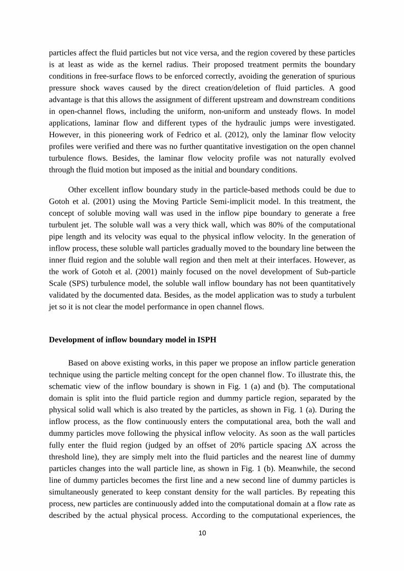
Based on above existing works, in this paper we propose an inflow particle generation

technique using the particle melting concept for the open channel flow. To illustrate this, the

schematic view of the inflow boundary is shown in Fig. 1 (a) and (b). The computational

domain is split into the fluid particle region and dummy particle region, separated by the

physical solid wall which is also treated by the particles, as shown in Fig. 1 (a). During the

inflow process, as the flow continuously enters the computational area, both the wall and

dummy particles move following the physical inflow velocity. As soon as the wall particles

fully enter the fluid region (judged by an offset of 20% particle spacing X across the

threshold line), they are simply melt into the fluid particles and the nearest line of dummy

particles changes into the wall particle line, as shown in Fig. 1 (b). Meanwhile, the second

line of dummy particles becomes the first line and a new second line of dummy particles is

simultaneously generated to keep constant density for the wall particles. By repeating this

process, new particles are continuously added into the computational domain at a flow rate as

described by the actual physical process. According to the computational experiences, the

11

offset value 20% ~ 30% could provide the best inflow simulation. However, instability of the

inflow particles can occur if this value is more than that.

Fig. 1 (a) and (b) Treatment of inflow boundary using the particle melting technique

New dummy particles

New fluid particles

(b)

New wall particles

Wall particles

Fluid particles Dummy particles

Inflow

(a)

12

During the inflow generation, the wall and dummy particles are moved with a uniform

velocity that is the same as the real channel depth-averaged velocity. The pressures of wall

particles are solved by the PPE equation (12), while the dummy particle pressures are not

solved but set equal to the pressures of corresponding wall particles in the horizontal normal

direction. In this sense, homogeneous pressure boundary condition xP = 0 is imposed as

the inflow boundary condition. One common approach to treat the outflow boundary condition is to treat it as the open

boundary. That is to say, the physical properties of the fluid particles leaving the

computational domain are frozen except that their spatial positions are updated with the flow.

Then they can be simply removed from the computational domain after passing through a

threshold boundary region which is longer than the kernel impact range. Similar outflow

boundary treatment was also used by Federico et al. (2012). Although more complex outflow

boundary conditions can be described like the inflow boundary, this is not the main focus of

the present work. More advanced outflow boundary models were also provided by Federico

et al. (2012).

Evaluations of ISPH inflow model

The present ISPH inflow boundary model is based on the soluble wall concept of Gotoh

et al. (2001) in principle. However, the difference is that in Gotoh et al. (2001), the soluble

walls included only the dummy particles which were moved during the inflow generation,

while the fixed wall particles were kept stationary until the soluble particles crossed it.

Although Gotoh et al. (2001) proposed the earliest inflow boundary technique based on the

particle models, no detailed follow-on works have been carried out to evaluate the efficiency

and accuracy of their inflow model. Only the general flow behaviours were satisfactorily

reproduced but in-depth validation and analysis of the fundamental velocity profiles were not

carried out.

In Federico et al. (2012), they directly assigned the specified velocity and pressure

profiles to the inflow particles. In some sense, we could explain that in Federico et al. (2012),

the pressure boundary condition has to be prescribed because the WCSPH they used deals

with the pressure explicitly. On the other hand, the ISPH handles the pressure implicitly by

solving the pressure Poisson equation and thus the pressure gradient condition xP = 0

should be more appropriate. However, in many practical open channel flows the inflow

velocity and pressure distributions may not be exactly known at the beginning and it would

be impossible to set a specified profile for these. Therefore, the proposed ISPH inflow

boundary model is more general in that it does not need the detailed flow parameter

distributions on the inflow boundary and can be applied to more complex flow situations.

Also, in Federico et al. (2012), the model verification was based on the fact that, the initial

13

inner velocity field, which was initialized with the analytical solutions and updated by the

upstream inflow boundary conditions which were also initialized by the analytical solutions,

could be stably maintained or not during the computations. In comparison, in the proposed

ISPH inflow model we generate the open channel flows following the channel bed

topography so the flow velocity profiles are naturally evolved. Similar to Federico et al.

(2012), not only the uniform flow, but also the non-uniform and non-steady flows can also be

easily generated by the present ISPH model, for example, by adjusting the height of the

soluble wall or by using the time-dependent velocity to move the wall and dummy particles.

Laminar Flow Applications

Model setup and computational parameters

In this section, the proposed ISPH inflow model is applied to a viscous uniform laminar

flow in a laboratory scale. The computational model specifications are as follows: The main

numerical channel flume is 1.2 m long and 0.5 m high. Two different flow depths are studied,

i.e. d = 0.1 m and 0.2 m. The corresponding channel bed slopes are 0S = 0.04% and 0.1%,

and the fluid viscosities are 0 = 10-4 m2/s and 6 × 10-4 m2/s, respectively, for the two flow

depths. By balancing the computational efficiency and accuracy, a particle spacing of X =

0.005 m is adopted. This particle resolution guarantees that 20 ~ 40 particles are placed along

the vertical flow depth to minimize the channel bed boundary effect. There are around 5000

and 10000 particles involved in the ISPH computations for the two different flow depths. The

flow Reynolds number 0max /Re dU is evaluated by using the maximum flow velocity on

the free surface. Thus the two flows with d = 0.1 m and 0.2 m fall into the laminar regime

with Re numbers being around 200 and 100, which is consistent with the Re number ranges

investigated by Federico et al. (2012).

On the channel bed, a non-slip solid boundary condition is imposed by one layer of

fixed and two layers of dummy particles following Koshizuka et al. (1998). The free surfaces

are judged by using the particle density during the computation. Numerical simulations are

carried out for sufficient time to allow the fluid particles entering the channel inlet to pass

through the whole fluid domain. The particles in the fluid region are set static at the

beginning of the computation while a uniform seeding velocity is given to the inflow particles

which include the wall and dummy particles.

14

Flow velocity analysis

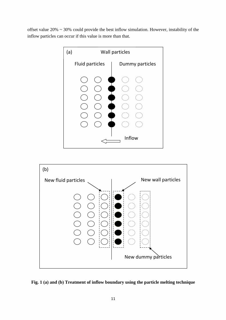
According to the ISPH computations, Fig. 2 (a) and (b) show the particle velocity

contours in a steady state 10 seconds after the flow is initiated, for the flow depth of 0.1 m

and 0.2 m, respectively. As expected for a typical viscous laminar regime, it shows that the

flow develops in almost parallel layers with an ordered particle distribution. The simulated

flow patterns are very similar to those described by Federico et al. (2012) based on the

WCSPH approach. The present ISPH computations show the stable situations until the

normalized time scale 2/1)/( dgt reaches 70 and 100 for the two flow depths, which is also

close to the timescale used by Federico et al. (2012). The proposed inflow/outflow boundary

treatment in ISPH allows the simulation to proceed up to Re number 200. The robustness of

the numerical algorithm is fully demonstrated in Fig. 2, where the streamlines of the flow and

the parabolic velocity fields are well preserved.

Fig. 2 ISPH computed uniform laminar flow particle velocity contours at flow depth of

(a) 0.1 m; and (b) 0.2 m

15

Here we need to mention that the inflow particles as shown in Fig. 1 are moved using a

uniform horizontal velocity on the inflow boundary based on a feeding velocity which can be

easily estimated by the standard open channel hydraulics. Then after the particles have melt

inside the fluid region, their velocities are adjusted following the channel bed slope and local

topography, until a final parabolic velocity profile is gradually evolved. The velocity contours

in Fig. 2 actually show the flow situations after the stable velocity profile has been developed.

Therefore, the computational domain length of 1.2 m as mentioned in the previous section did

not include the extra space in which the flow velocity developed from a constant profile to a

parabolic one. This imposition of the constant inflow particle velocity in present ISPH model

is different from that used by Federico et al. (2012) who had already used the eventual

parabolic velocity profile in the inflow region.

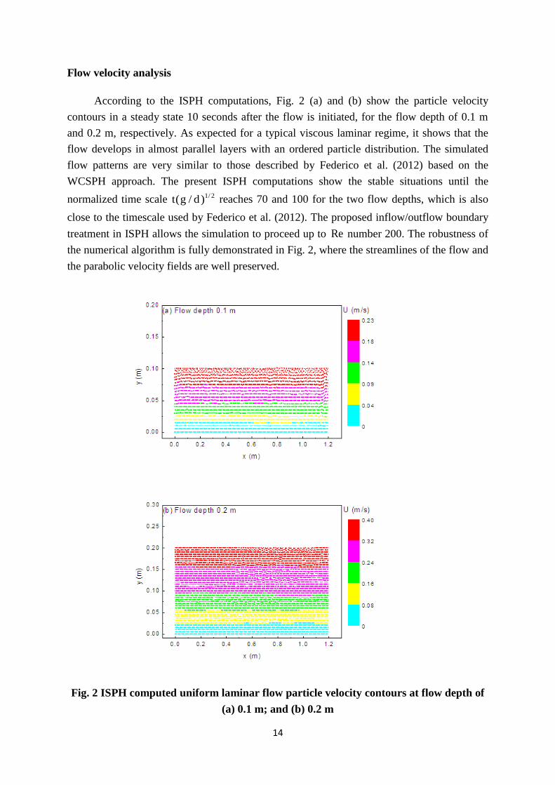
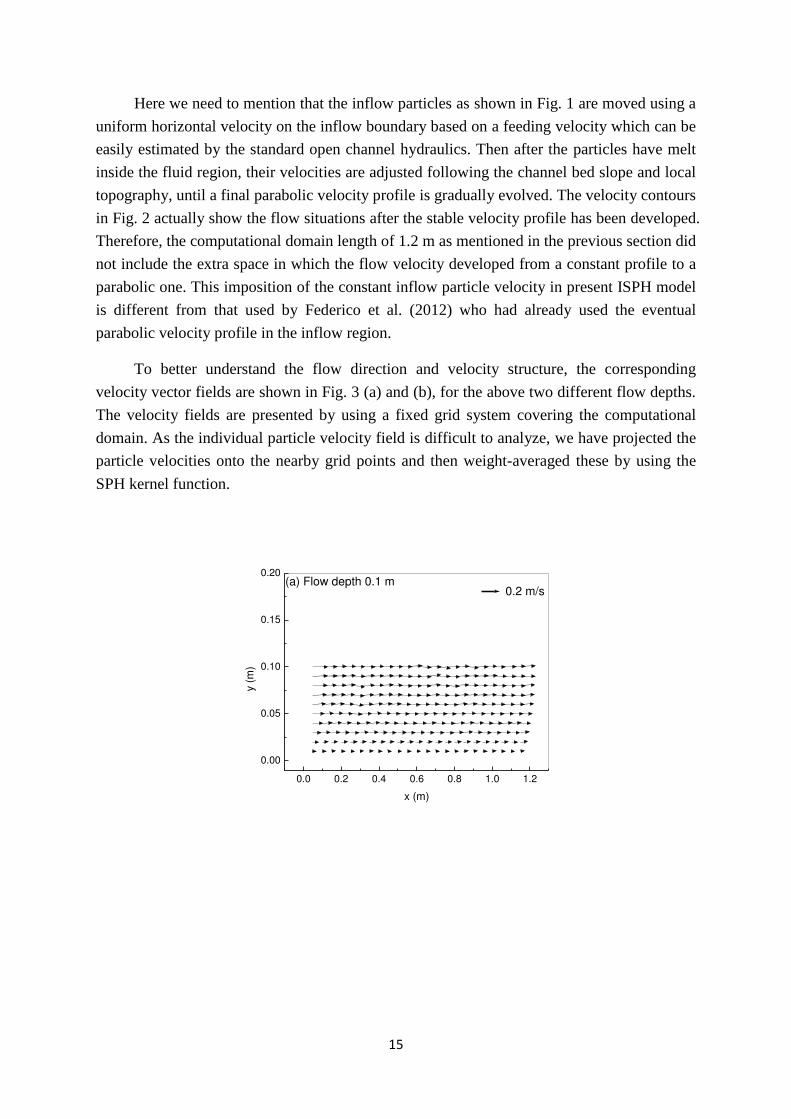
To better understand the flow direction and velocity structure, the corresponding

velocity vector fields are shown in Fig. 3 (a) and (b), for the above two different flow depths.

The velocity fields are presented by using a fixed grid system covering the computational

domain. As the individual particle velocity field is difficult to analyze, we have projected the

particle velocities onto the nearby grid points and then weight-averaged these by using the

SPH kernel function.

0.0 0.2 0.4 0.6 0.8 1.0 1.2

0.00

0.05

0.10

0.15

0.20

0.2 m/s(a) Flow depth 0.1 m

y (m

)

x (m)

16

Fig. 3 ISPH computed uniform laminar flow velocity vector field at flow depth of (a) 0.1

m; and (b) 0.2 m

The theoretical velocity profile for a 2D uniform, steady and laminar flow in a free-

surface channel is given by the following equation:

])(2

1[2 2

max d

y

d

y

U

U (20)

in which U = velocity distribution in the vertical location y ; d = flow depth; and maxU =

maximum flow velocity on the free surface, which can be determined by the analytical formula for the Poiseuille flow as provided by Federico et al. (2012).

To quantify the ISPH inflow model performance, the numerical results are compared

with the analytical solution for the vertical velocity profile at middle section of the flume in

Fig. 4 (a) and (b), at the flow depth of 0.1 m and 0.2 m. It is found that a very satisfactory

agreement has been achieved. Equally good results were also reported by Federico et al.

(2012), but their studies aimed to find out whether the velocity profiles that had been

initialized with the analytical solutions and updated by the upstream inflow boundary

conditions, could be maintained for a long enough time or not. In comparison, our present

ISPH velocity profiles have been naturally developed from the computations based on a zero

initial velocity field and a constant inflow velocity boundary.

0.0 0.2 0.4 0.6 0.8 1.0 1.2

0.00

0.05

0.10

0.15

0.20

0.25

0.30

0.35 m/s(b) Flow depth 0.2 m

y (m

)

x (m)

17

0.00 0.05 0.10 0.15 0.200.00

0.02

0.04

0.06

0.08

0.10

0.12(a) Flow depth 0.1 m

ISPH

Analytical

y (m

)

U (m/s)

0.00 0.05 0.10 0.15 0.20 0.25 0.30 0.350.00

0.04

0.08

0.12

0.16

0.20

0.24(b) Flow depth 0.2 m

ISPH

Analytical

y (m

)

U (m/s)

Fig. 4 Computed and analytical laminar flow velocity profiles at flow depth of (a) 0.1 m; and (b) 0.2 m

However, it should be noted that the simulation using flow depth d = 0.1 m generated

slightly larger errors near the channel bed as shown in Fig. 4 (a). This could be attributed to

the shallow flow conditions and the ISPH solid boundary treatment, which induced the

artificial drag force on the solid walls. This did not influence the flow velocity profile away

from the bed because it was in the laminar flow regime. The problem seems to become more

serious in the following turbulent flow situation.

18

Turbulent Flow Applications

Flow velocity analysis

Having been verified for the laminar flow, in this section the ISPH model is applied to

an open channel uniform turbulent flow at flow depth of d = 0.1 m, 0.2 m and 0.4 m,

respectively. The computational model is the same as that used in the laminar flow test,

except that the flow viscosity is taken as 0 = 10-6 m2/s. Here the real water viscosity is used

in order to generate a fully turbulent flow with the Reynolds number reaching 150000. The

inflow is generated by moving the wall and dummy particles of the inflow region (with

height of 0.1 m, 0.2 m and 0.4 m, respectively) at a constant feeding speed which is larger

than zero. It was found in the computations that a seeding velocity of 0.1 ~ 0.6 m/s makes no

much difference for the final stable inner velocity profile in this case study, although the

length of the velocity adjustment region could differ. The outflow boundary is treated as the

open boundary, that is to say, the particle properties are frozen and their exit velocities are

maintained until they move out of the computational domain, similar to the outflow boundary

model used by Federico et al. (2012).

According to the ISPH computation, the particle velocity contours and vector fields in a

steady flow state are shown in Fig. 5 (a) and (b), respectively, for the flow depth of d = 0.4

m. Different from the laminar flow as shown in Fig. 2 and 3, the turbulent flow demonstrates

a much more random and disordered particle motion, with extensive particle mixing near the

interface of different velocity layers. Although the XSPH variant was used in the model,

some kinds of flow fluctuation are observed near the free surface and the bed boundary as

shown in Fig. 5 (b). We attributed this to the inherent fluctuation of the turbulent flows.

Without using the XSPH variant, there would have been no stable flow circulations obtained.

0.0 0.2 0.4 0.6 0.8 1.0 1.2

0.0

0.1

0.2

0.3

0.4

0.5

0.6U (m/s)(a) Particle velocity contour

y (m

)

x (m)

0

0.08

0.16

0.24

0.32

0.40

19

Fig. 5 ISPH computed uniform turbulent flow at flow depth of d = 0.4 m. (a) Particle

velocity contour; and (b) Velocity vector field

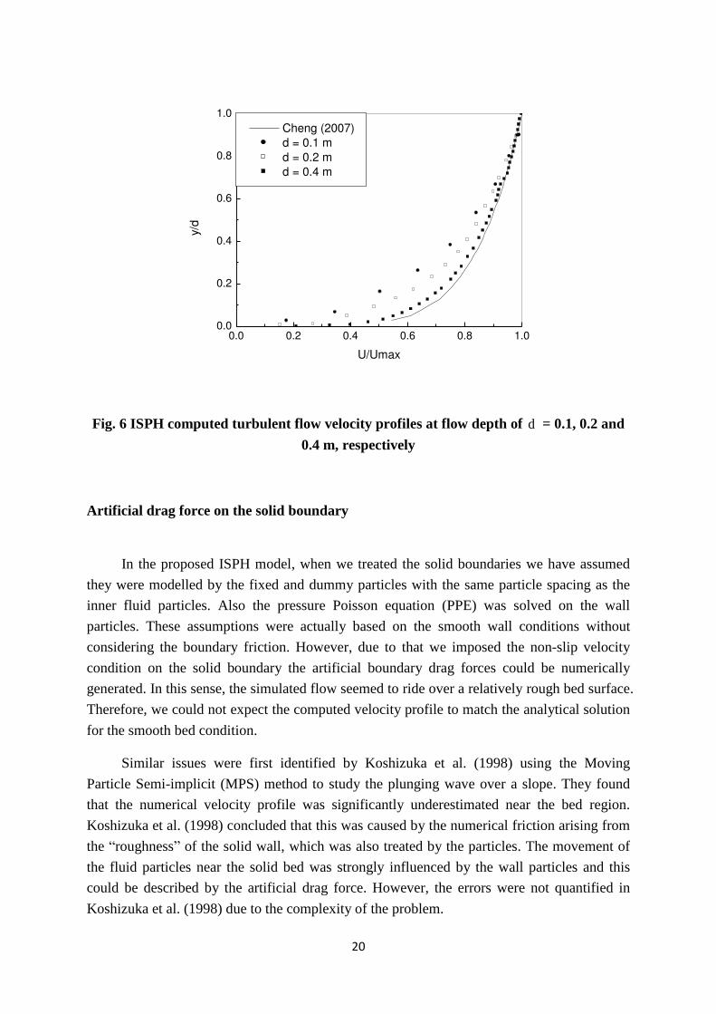
To verify the ISPH turbulent flow simulation, the computed flow velocity profiles for

flow depth of d = 0.1, 0.2 and 0.4 m, are compared with the semi-analytical solutions of

Cheng (2007) in Fig. 6, in which the normalized analytical velocity profile is represented by

m

d

y

U

U/1

max

(21)

where the power index m = 6 is used to describe the turbulent flow over a relatively smooth

bed in Cheng (2007). maxU is the maximum flow velocity computed/measured on the free

surface. In Cheng’s (2007) study, it was found that the power law could be applied to a larger

fraction of the flow domain in the open channel flow as compared with the more theoretical

and complex log law, which only applies to the near bed region in principle. By the attempts

to show that the power law can be derived as a first-order approximation to the log law, and

its power-law index is computed as a function of the Reynolds number as well as the relative

roughness height, the novel work of Cheng (2007) derived a general power law formulation

to describe the open channel flow with a wide range of bed roughness.

However, the comparisons in Fig. 6 indicate quite large errors near the channel bed,

although the overall velocity trend in the upper band of the profile is quite promising. Besides,

Fig. 6 also demonstrates that as the flow depth becomes deeper, such as d = 0.4 m, the

agreement with the semi-analytical solution (Cheng, 2007) becomes better as compared with

the shallow flow condition. We will make further investigation on this phenomenon as below.

0.0 0.2 0.4 0.6 0.8 1.0 1.2

0.0

0.1

0.2

0.3

0.4

0.5

0.6

0.4 m/s(b) Velocity vector field

y (m

)

x (m)

20

0.0 0.2 0.4 0.6 0.8 1.00.0

0.2

0.4

0.6

0.8

1.0

Cheng (2007)

d = 0.1 m

d = 0.2 m

d = 0.4 m

y/d

U/Umax

Fig. 6 ISPH computed turbulent flow velocity profiles at flow depth of d = 0.1, 0.2 and

0.4 m, respectively

Artificial drag force on the solid boundary

In the proposed ISPH model, when we treated the solid boundaries we have assumed

they were modelled by the fixed and dummy particles with the same particle spacing as the

inner fluid particles. Also the pressure Poisson equation (PPE) was solved on the wall

particles. These assumptions were actually based on the smooth wall conditions without

considering the boundary friction. However, due to that we imposed the non-slip velocity

condition on the solid boundary the artificial boundary drag forces could be numerically

generated. In this sense, the simulated flow seemed to ride over a relatively rough bed surface.

Therefore, we could not expect the computed velocity profile to match the analytical solution

for the smooth bed condition.

Similar issues were first identified by Koshizuka et al. (1998) using the Moving

Particle Semi-implicit (MPS) method to study the plunging wave over a slope. They found

that the numerical velocity profile was significantly underestimated near the bed region.

Koshizuka et al. (1998) concluded that this was caused by the numerical friction arising from

the “roughness” of the solid wall, which was also treated by the particles. The movement of

the fluid particles near the solid bed was strongly influenced by the wall particles and this

could be described by the artificial drag force. However, the errors were not quantified in

Koshizuka et al. (1998) due to the complexity of the problem.

21

To numerically support the above analysis, the ISPH computed velocity profiles for

three different flow depths are fitted to the semi-analytical results for the rough bed turbulent

flows (Cheng, 2007) in Fig. 7. Following Cheng (2007), the difference between the smooth

and rough bed turbulent flow velocity profiles can be reflected by the index m in Eq. (21)

and a smaller m indicates a more rough bed condition with higher artificial drag force. The

fittings of the numerical and analytical velocity curves are based on the minimum averaged

errors between the two results. Fig. 7 shows that the power index m decreases from 6.0 for

the most smooth bed, to 5.3 for the flow depth d = 0.4 m, and down to 2.9 for the most

shallow depth d = 0.1 m. It suggests that when the flow depth d becomes smaller (which is

equivalent to a larger particle spacing X ), the flow is more likely to ride over a numerically

rough bed because the influence of the solid boundary becomes more substantial. This could

explain the situation that the ISPH computation by using flow depth d = 0.4 m is closer to

the analytical result for a smooth bed (Cheng, 2007). Further investigations will be made in

the next section, in which the ISPH computation using a smaller particle spacing X can

match the m = 6.0 curve quite well.

0.0 0.2 0.4 0.6 0.8 1.00.0

0.2

0.4

0.6

0.8

1.0

Cheng (2007) m=5.3

Cheng (2007) m=3.8

Cheng (2007) m=2.9

d = 0.1 m

d = 0.2 m

d = 0.4 m

y/d

U/Umax

Fig. 7 Fittings of the ISPH computed and semi-analytical (Cheng, 2007) velocity profiles

Here it should be realized that in the laminar and some transient unsteady flows, such

as the wave breaking and dam collapse, the influence of the artificial boundary drag force is

not as obvious as what we have found in the above uniform turbulent flow. This is because

the simulation time of these instantaneous unsteady flows is relatively short, so the boundary

drag force could not obtain a sufficient time scale to generate the substantial impact on the

numerical result.

22

Convergence Analysis of Numerical Scheme

In this section, we use a series of numerical runs based on different particle spacings

X and time steps t to evaluate the accuracy and convergence of the ISPH model in open

channel flow applications.

Model accuracy in the spatial domain

To quantify the accuracy of the ISPH numerical scheme in the spatial domain,

additional two runs with a coarser and finer particle spacing are implemented, i.e. X = 0.01

m and 0.0025 m, as compared with the original run in which X = 0.005 m was used. The

computational time step t is maintained the same for all the tests for consistency.

The order of convergence of the numerical scheme can be quantitatively determined by

the differences among the three numerical results. Similar approach has also been employed

by Ogami (1999) for analyzing his Lagrangian scheme in a compressible flow application. In

this work, the numerical error XE was proportional to the particle spacing by CRX)( ,

where CR was the order of convergence. By assuming 005.0,01.0E and 0025.0,005.0E as the

numerical errors between the runs using particle spacing X = (0.01 m, 0.005 m) and (0.005

m, 0.0025 m), respectively, then the following relationship can be established

CR

XX

XX

E

E)(

0025.0005.0

005.001.0

0025.0,005.0

005.0,01.0

(22)

According to the design of the numerical test, we have

0025.0005.001.0 42 XXX (23)

So Equation (22) is simplified to

CR

E

E2

0025.0,005.0

005.0,01.0 (24)

Based on the above principle, a series of numerical tests are carried out for the laminar

and turbulent flow velocity profiles and the results are shown in Fig. 8 (a) and (b),

respectively. The laminar flow uses the flow depth of d = 0.2 m and the turbulent flow depth

is d = 0.4 m. The figures show that the numerical differences between the two refined runs

are much smaller than those between the two coarser runs, indicating the convergence of the

numerical scheme. By using 40 points from each subfigure, the convergence index CR is

worked out to be 1.25 for the laminar flow and 1.05 for the turbulent one. This suggested that

23

the accuracy of the proposed ISPH model falls into )( XO and )( 2XO in the spatial

domain.

0.00 0.05 0.10 0.15 0.20 0.25 0.30 0.350.00

0.04

0.08

0.12

0.16

0.20

0.24

X=0.01 m

X=0.005 m

X=0.0025 m

(a) Laminar flow

y (m

)

U (m/s)

0.0 0.2 0.4 0.6 0.8 1.00.0

0.2

0.4

0.6

0.8

1.0

X=0.01 m

X=0.005 m

X=0.0025 m

(b) Turbulent flow

y/d

U/Umax

Fig. 8 Convergence test of ISPH numerical scheme in the spatial domain. (a) Laminar flow; and (b) Turbulent flow

24

Model accuracy in the temporal domain

To study the accuracy of numerical scheme in the time domain, additional two runs

with a finer and coarser time step t = 0.0001 and 0.0004 s are used, in comparison with the

original run using t = 0.0002 s. For all of the three runs, the particle spacing X = 0.005 m

is kept unchanged to have a consistent spatial resolution.

For the evaluation of the model convergence, similar analysis as employed in the

previous section is used. By assuming that the numerical errors tE are proportional to

CRt)( , a useful relationship analogous to Equation (22) can be established to relate the

numerical errors with the time steps as

CR

tt

tt

E

E)(

0001.00002.0

0002.00004.0

0001.0,0002.0

0002.0,0004.0

(25)

and also being due to

0001.00002.00004.0 42 ttt (26)

So we can have

CR

E

E2

0001.0,0002.0

0002.0,0004.0 (27)

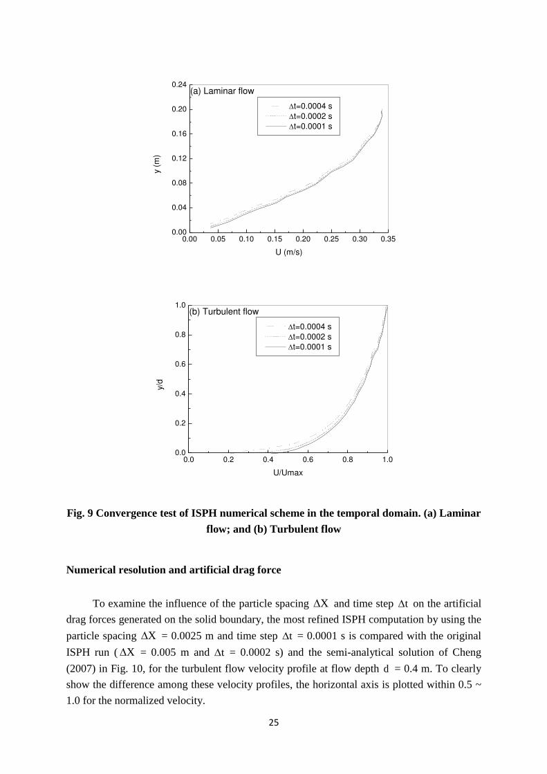
The numerical tests are carried out again for the laminar and turbulent flow velocity

profiles and the results are shown in Fig. 9 (a) and (b), respectively. Convergence of the

numerical scheme with the time step t is obvious in that the differences between the two

refined runs are smaller than those between the two coarser runs.

Again by using 40 points from each subfigure, the power index CR is calculated to be

1.02 and 0.98, respectively, for the laminar and turbulent flow conditions. This suggested that

the numerical accuracy of the model is around )( tO in the temporal domain. Here there is

no much difference observed in the convergence behaviours between the laminar and

turbulent flows. This is due to that the particle disorders, which could have a large effect on

the spatial accuracy of the turbulent flows, may not have much influence in the temporal

resolutions.

25

0.00 0.05 0.10 0.15 0.20 0.25 0.30 0.350.00

0.04

0.08

0.12

0.16

0.20

0.24

t=0.0004 s

t=0.0002 s

t=0.0001 s

(a) Laminar flow

y (m

)

U (m/s)

0.0 0.2 0.4 0.6 0.8 1.00.0

0.2

0.4

0.6

0.8

1.0

t=0.0004 s

t=0.0002 s

t=0.0001 s

(b) Turbulent flow

y/d

U/Umax

Fig. 9 Convergence test of ISPH numerical scheme in the temporal domain. (a) Laminar

flow; and (b) Turbulent flow

Numerical resolution and artificial drag force

To examine the influence of the particle spacing X and time step t on the artificial

drag forces generated on the solid boundary, the most refined ISPH computation by using the

particle spacing X = 0.0025 m and time step t = 0.0001 s is compared with the original

ISPH run ( X = 0.005 m and t = 0.0002 s) and the semi-analytical solution of Cheng

(2007) in Fig. 10, for the turbulent flow velocity profile at flow depth d = 0.4 m. To clearly

show the difference among these velocity profiles, the horizontal axis is plotted within 0.5 ~

1.0 for the normalized velocity.

26

0.5 0.6 0.7 0.8 0.9 1.00.0

0.2

0.4

0.6

0.8

1.0

Original

Time refined

Space refined

Cheng (2007)y/

d

U/Umax

Fig. 10 Comparisons of turbulent flow velocity profile between the original and two

refined ISPH results and semi-analytical solution of Cheng (2007)

Fig. 10 shows that as either the particle spacing X or the time step t becomes

smaller, the computed velocity profile becomes closer to the result of Cheng (2007).

However, the computation based on the refined particle spacing gives a much more

satisfactory match than that based on the refined time step. This indicates that the artificial

boundary drag forces are not pronounced in the simulation of flows with large depth as more

particles exist in the vertical direction of the flow. On the other hand, employing a refined

temporal resolution can also improve the simulation accuracy near the solid boundary to

some extent.

27

Conclusions

The paper presents an improved ISPH inflow boundary method to simulate open

channel flow. The main purpose of the work aims to verify the velocity profile of uniform

laminar and turbulent flows and evaluate the ISPH stability and accuracy. One contribution of

the work is that the computed velocity profiles are not prescribed but naturally evolved

during the flow process by following the channel bed configuration. In the inflow region only

a constant feeding velocity is provided and the pressure boundary condition is simply

embedded in the ISPH pressure equation for the wall and dummy particles. So much less

flow information is needed for the inflow region as compared with other particle modelling

approaches. Another useful contribution is that we found the standard SPH treatment of

smooth solid boundaries by using the fixed particle could generate numerical artificial drag

forces and we tentatively quantified its influence by using the semi-empirical solution of a

turbulent flow (Cheng, 2007). Furthermore, it has also been found that by increasing the flow

depth or decreasing the particle spacing it can effectively improve the simulation accuracy

near the bed, which is consistent with the MPS simulations of open channel flow by Fu and

Jin (2013). The convergence analysis indicated that the proposed ISPH model is globally

first-order accurate in both the spatial and temporal domains.

As further evaluation of the model, two additional computations are carried out in the

following Appendixes. The first one uses an alternative solid boundary treatment based on

the mirroring particle method, in which the outer-boundary dummy particles are not fixed but

a reflection of the inner fluid particles near the solid boundary. The control simulation has

indicated a very promising improvement in the reduction of the artificial boundary drag

forces and achieved much better agreement in the velocity profiles with documented data.

Then the model is applied to one more robust test of open channel flow over a complex bed.

Moreover, it has been found that the pressure distributions in the inflow region demonstrated

a quite stable pattern without large pressure noises.

Acknowledgements

This research work is supported by the Maritime Research Centre, Nanyang

Technological University and the Tan Chin Tuan Exchange Fellowship (Inbound) FY2011. S.

Shao also acknowledges the support of the Major State Basic Research Development

Program (973 Program) of China (No. 2013CB036402) and the National Natural Science

Foundation of China (NSFC No. 51479087). Dr Min Luo from the National University of

Singapore contributed to the data processing during the revision of the manuscript.

28

Appendix I Reduction of Artificial Boundary Drag Forces

As mentioned before, the existence of artificial boundary drag forces severely

influenced the simulation accuracy of the turbulent flow and led to a numerically smaller

velocity profile near the bed. We have mentioned that this could be caused by the treatment

of the solid bed using the fixed wall particles and the assumption of the non-slip boundary

conditions. In this section, we use an alternative procedure to treat the solid boundary, i.e. the

mirroring particle method, so a free-slip boundary condition can be easily imposed. The

mirroring rules were first presented by Cummins and Rudman (1999) in an SPH projection

method but this has been extensively improved by many follow-on SPH works, such as Liu et

al. (2013) for the more complex moving solid boundaries. In this paper, we only apply the

original mirroring rules of Cummins and Rudman (1999) since the main objective is to

investigate its effect on reducing or removing the artificial boundary drag forces.

Again by using the above turbulence flow case with the flow depth d = 0.1, 0.2 and 0.4

m and the particle spacing X = 0.005 m, we re-computed the flow velocity profiles by

using the mirroring particle approach to impose a free-slip boundary condition and compared

with the semi-analytical solution of Cheng (2007), which is shown in Fig. A1. Compared

with the results in Fig. 6, in which the non-slip ISPH model was used, it demonstrates that the

imposition of the free-slip boundary condition has been very effective in reducing the effect

of the artificial boundary drag forces so the computed near-bed velocity profiles match much

better with Cheng (2007) than the non-slip computations. However, we have to realize that

there still exist some kinds of discrepancies near the bed which require further investigation.

0.0 0.2 0.4 0.6 0.8 1.00.0

0.2

0.4

0.6

0.8

1.0

Cheng (2007)

d = 0.1 m

d = 0.2 m

d = 0.4 m

y/d

U/Umax

Fig. A1 ISPH computed turbulent flow velocity profiles at flow depth of d = 0.1, 0.2 and

0.4 m, by using mirroring particle treatment of the channel bed

29

Appendix II Open Channel Flow over a Complex Bed

To further investigate the model application in more complex open channel flows, we

apply the ISPH inflow model to an open channel flow over a trapezoidal trench based on the

experiment of Alfrink and van Rijn (1983). The trench is located perpendicular to the flow

direction and more details on the experimental work can be found in their original paper. This

simulation has also been done by Shakibaeinia and Jin (2011) using the Moving Particle

Semi-implicit (MPS) method. To be consistent with the MPS computation, the ISPH particle

spacing is selected as 0.01 m to ensure 40 particles in the depth direction in the middle of the

trench to satisfy the computational accuracy. Three measurement sections are located in the

middle of the two down slopes as well as the horizontal section for the model validation.

Following Shakibaeinia and Jin (2011), the ISPH numerical results were also taken after 10 s

when the flow had reached nearly stable condition. A schematic setup of the numerical flume

and three measurement sections are shown in Fig. A2.

-1.5 -1.0 -0.5 0.0 0.5 1.0 1.5

0.0

0.2

0.4

0.6S3S1 S2

y (m

)

x (m)

Fig. A2 Schematic setup of numerical flume and measurement sections for open channel trench flow

Fig. A3 (a) ~ (c) shows the comparison between the ISPH numerical results and

experimental data of Alfrink and van Rijn (1983) for the longitudinal flow velocities in three

cross-sections as mentioned above. A generally good agreement has been found and the

model is shown to be able to accurately simulate the velocity distribution in the areas with

complex reversed flows. This has been caused by the flow separation and circulation arising

from the influence of the trench. Here it should be noted that the flow velocity profiles near

the channel bed are also well reproduced by the numerical model, which is in sharp contrast

with the previous open channel turbulent flow profiles in Fig. 6. The reason is attributed to

that in the present case the numerical results are compared with the experimental data

collected from a real channel bed with the physical roughness, whereas in the previous

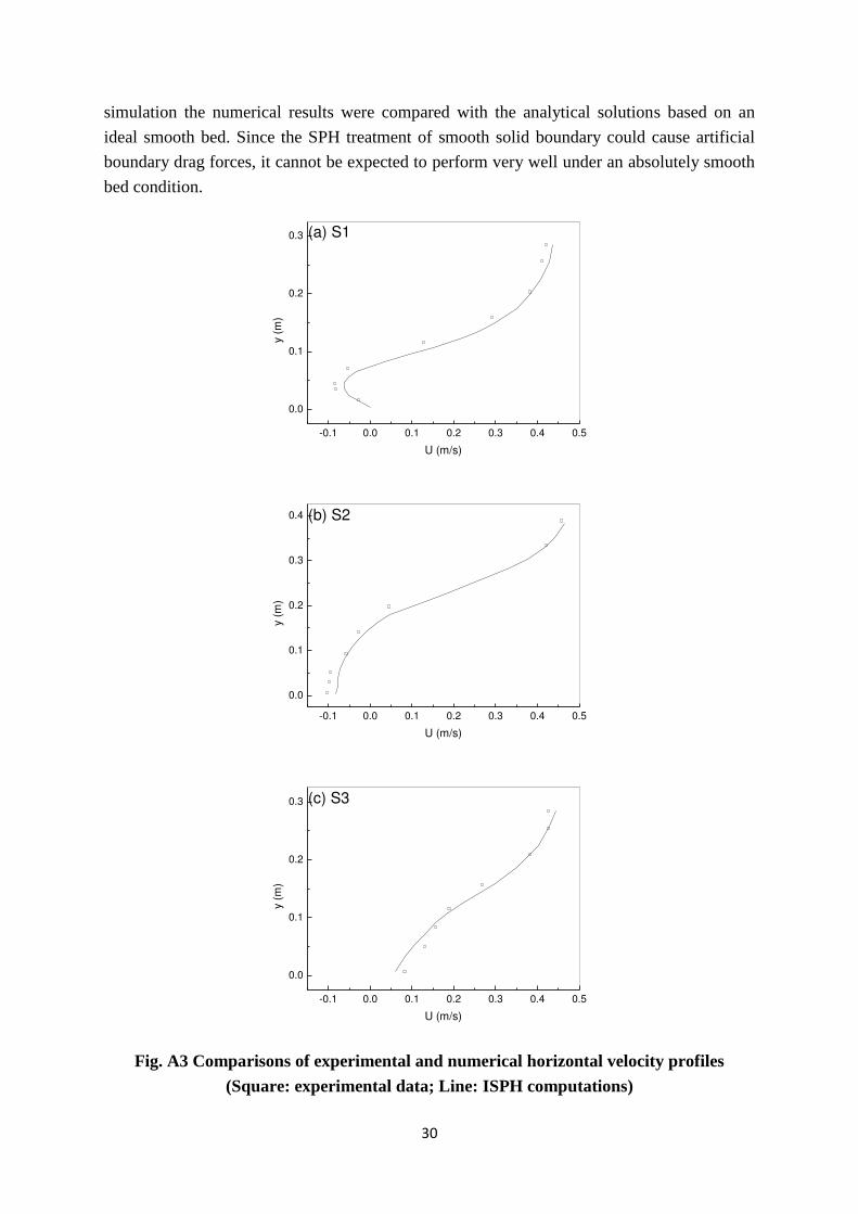
30

simulation the numerical results were compared with the analytical solutions based on an

ideal smooth bed. Since the SPH treatment of smooth solid boundary could cause artificial

boundary drag forces, it cannot be expected to perform very well under an absolutely smooth

bed condition.

-0.1 0.0 0.1 0.2 0.3 0.4 0.5

0.0

0.1

0.2

0.3 (a) S1

y (m

)

U (m/s)

-0.1 0.0 0.1 0.2 0.3 0.4 0.5

0.0

0.1

0.2

0.3

0.4 (b) S2

y (m

)

U (m/s)

-0.1 0.0 0.1 0.2 0.3 0.4 0.5

0.0

0.1

0.2

0.3 (c) S3

y (m

)

U (m/s)

Fig. A3 Comparisons of experimental and numerical horizontal velocity profiles

(Square: experimental data; Line: ISPH computations)

31

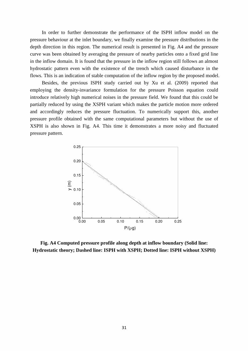
In order to further demonstrate the performance of the ISPH inflow model on the

pressure behaviour at the inlet boundary, we finally examine the pressure distributions in the

depth direction in this region. The numerical result is presented in Fig. A4 and the pressure

curve was been obtained by averaging the pressure of nearby particles onto a fixed grid line

in the inflow domain. It is found that the pressure in the inflow region still follows an almost

hydrostatic pattern even with the existence of the trench which caused disturbance in the

flows. This is an indication of stable computation of the inflow region by the proposed model.

Besides, the previous ISPH study carried out by Xu et al. (2009) reported that

employing the density-invariance formulation for the pressure Poisson equation could

introduce relatively high numerical noises in the pressure field. We found that this could be

partially reduced by using the XSPH variant which makes the particle motion more ordered

and accordingly reduces the pressure fluctuation. To numerically support this, another

pressure profile obtained with the same computational parameters but without the use of

XSPH is also shown in Fig. A4. This time it demonstrates a more noisy and fluctuated

pressure pattern.

0.00 0.05 0.10 0.15 0.20 0.250.00

0.05

0.10

0.15

0.20

0.25

y (

m)

P/(g)

Fig. A4 Computed pressure profile along depth at inflow boundary (Solid line: Hydrostatic theory; Dashed line: ISPH with XSPH; Dotted line: ISPH without XSPH)

32

References

Afshar, M. H. and Shobeyri, G. (2010), Efficient simulation of free surface flows with discrete least-squares meshless method using a priori error estimator, Int. J. Comput. Fluid Dyn., 24, 349-367.

Alfrink, B. J. and van Rijn, L. C. (1983), Two-equation turbulence model for flow in trenches,

J. Hydraul. Eng., ASCE, 109(7), 941–958.

Ataie-Ashtiani, B. and Shobeyri, G. (2008), Numerical simulation of landslide impulsive

waves by incompressible smoothed particle hydrodynamics, Int. J. Numer. Meth. Fluids, 56, 209–232.

Cheng, N. S. (2007), Power-law index for velocity profiles in open channel flows, Adv.

Water Resour., 30, 1775–1784. Cummins, S. J. and Rudman, M. (1999), An SPH projection method, J. Comp. Phys., 152,

584-607. Dalrymple, R. A. and Rogers, B. D. (2006), Numerical modeling of water waves with the

SPH method, Coast. Eng., 53, 141-147. Federico, I., Marrone, S., Colagrossi, A., Aristodemo, F. and Antuono, M. (2012), Simulating

2D open-channel flows through an SPH model, European J. Mech. B/Fluids, 34, 35-46.

Fu, L. and Jin, Y. C. (2013), A mesh-free method boundary condition technique in open channel flow simulation, Journal of Hydraulic Research, 51(2), 174–185.

Gomez-Gesteira, M., Cerqueiroa, D., Crespoa, C. and Dalrymple, R. A. (2005), Green water

overtopping analyzed with a SPH model, Ocean Eng., 32, 223-238. Gotoh, H., Shibahara, T. and Sakai, T. (2001), Sub-particle-scale turbulence model for the

MPS method – Lagrangian flow model for hydraulic engineering, Comp. Fluid Dyn. J., 9, 339-347.

Koshizuka, S., Nobe, A. and Oka, Y. (1998), Numerical analysis of breaking waves using the

moving particle semi-implicit method, Int. J. Numer. Meth. Fluids, 26, 751-769. Lastiwka, M., Basa, M. and Quinlan, N. J. (2009), Permeable and non-reflecting boundary

conditions in SPH, Int. J. Numer. Meth. Fluids, 61, 709–724.

33

Lee, E. S., Moulinec, C., Xu, R., Violeau, D., Laurence, D. and Stansby, P. (2008), Comparisons of weakly compressible and truly incompressible algorithms for the SPH mesh free particle method, J. Comput. Phys., 227, 8417-8436.

Liu, X., Xu, H. H., Shao, S. D. and Lin, P. Z. (2013), An improved incompressible SPH

model for simulation of wave-structure interaction, Computers & Fluids, 71, 113-123. Monaghan, J. J. (1992), Smoothed particle hydrodynamics, Annu. Rev. Astron. Astrophys.,

30, 543-574. Monaghan, J. J. and Kos, A. (1999), Solitary waves on a cretan beach, J. Wtrwy., Port,

Coastal and Ocean Eng., 125, 145-154. Ogami, Y. (1999), A pure Lagrangian method for unsteady compressible viscous flow, Comp.

Fluid Dyn. J., 8, 383-392. Oger, G., Doring, M., Alessandrini, B. and Ferrant, P. (2006), Two-dimensional SPH

simulations of wedge water entries, J. Comput. Phys., 213, 803–822. Rogers, B. D., Dalrymple, R. A. and Stansby, P. K. (2010), Simulation of caisson breakwater

movement using 2-D SPH, J. Hydr. Res., 48(Extra Issue), 135–141. Shakibaeinia, A. and Jin, Y. C. (2010), A weakly compressible MPS method for modeling of

open-boundary free-surface flow, Int. J. Numer. Meth. Fluids, 63, 1208–1232. Shakibaeinia, A. and Jin, Y. C. (2011), MPS-based mesh-free particle method for modeling

open-channel flows, Journal of Hydraulic Engineering, ASCE, 137(11), 1375-1384. Xu, R., Stansby, P. K. and Laurence, D. R. P. (2009), Accuracy and stability in projection

based method incompressible SPH (ISPH) and a new approach, Journal of Computational Physics, 228(18), 6703-6725.