Finance and Economics Discussion SeriesDivisions of Research & Statistics and Monetary Affairs

Federal Reserve Board, Washington, D.C.

Income Inequality, Financial Crises, and Monetary Policy

Isabel Cairo and Jae Sim

2018-048

Please cite this paper as:Cairo, Isabel, and Jae Sim (2018). “Income Inequality, Financial Crises, and Monetary Pol-icy,” Finance and Economics Discussion Series 2018-048. Washington: Board of Governorsof the Federal Reserve System, https://doi.org/10.17016/FEDS.2018.048.

NOTE: Staff working papers in the Finance and Economics Discussion Series (FEDS) are preliminarymaterials circulated to stimulate discussion and critical comment. The analysis and conclusions set forthare those of the authors and do not indicate concurrence by other members of the research staff or theBoard of Governors. References in publications to the Finance and Economics Discussion Series (other thanacknowledgement) should be cleared with the author(s) to protect the tentative character of these papers.

Income Inequality, Financial Crises,

and Monetary Policy∗

Isabel Cairo† Jae Sim‡

May 2018

Abstract

We construct a general equilibrium model in which income inequality results in insufficient aggregatedemand, deflation pressure, and excessive credit growth by allocating income to agents featuring lowmarginal propensity to consume, and if excessive, can lead to an endogenous financial crisis. Thiseconomy generates distributions for equilibrium prices and quantities that are highly skewed to thedownside due to financial crises and the liquidity trap. Consequently, symmetric monetary policyrules designed to minimize fluctuations around fixed means become inefficient. A simultaneousreduction in inflation volatility and mean unemployment rate is feasible when an asymmetric policyrule is adopted.

JEL Classification: E32, E44, E52, G01Keywords: income inequality, credit, financial crises, monetary policy

∗The analysis and conclusions set forth are those of the authors and do not indicate concurrence by other membersof the research staff or the Board of Governors. We thank Adrien Auclert, Robert Barsky, Larry Christiano, JamesCostain, Jordi Galı, Wouter den Haan, Michael Kumhof, Alberto Martin, Pascal Paul, and Federico Ravenna for valuablecomments and suggestions. We are also grateful to colleagues and to seminar and conference participants of USCDornsife, Annual Inflation Targeting Conference at the Banco Central Do Brasil, Empirical Macro Workshop at theUniversity of Ghent, Danmarks Nationalbank, the CEPR-ESSIM Conference at the Banco de Espana, the EuropeanCentral Bank/Bank of Canada Joint Annual Conference, the Federal Reserve Bank of Boston/CEBRA Joint Conference,the Society for Economic Dynamics, the Society for Computational Economics, the European Economic Association, theEuropean Winter Meeting of the Econometric Society, the Spanish Economic Association, the Board of Governors of theFederal Reserve System, the Federal Reserve Bank of Kansas City, and the Federal Reserve Bank of Chicago.†Board of Governors of the Federal Reserve System. Email: isabel.cairo@frb.gov‡Board of Governors of the Federal Reserve System. Email: jae.w.sim@frb.gov

“It’s revealing that in public debates, advocates for workers...have tended to favor the continua-

tion of easy money, while the typical op-ed about the adverse effects of easy money on the distribution

of income and wealth is written by a hedge fund manager, banker, or right-wing politician...That

political alignment—workers’ groups in support of easy money, financiers in favor of higher inter-

est rates—is of course the historical pattern in the United States, going back to William Jennings

Bryan and beyond.” – Bernanke (2017)

1 Introduction

The distribution of income in the United States has become more unequal over the last several decades,

reaching unprecedented levels as documented by Atkinson et al. (2011). While macroeconomic im-

plications of inequality have recently become the center of discussions by policymakers (Yellen, 2014;

Bernanke, 2017), the academic literature on the link among inequality, the macroeconomy, and mone-

tary policy is still in its infancy. This paper contributes to this literature by exploring a possibility that

income inequality may be at the root of many macroeconomic problems that the U.S. economy could

be facing such as secular stagnation, deflation pressure, excess credit growth, and financial crises. Us-

ing a novel theoretical model, we show that an economy suffering from such problems may be subject

to disproportionately large downside risks, making traditional monetary policy framework aiming to

minimize the volatilities of endogenous quantities and prices around fixed means inefficient. One of

the main contributions of this paper is to uncover robust monetary policy rules that can correct the

biases of the means due to the left-skewed distributions and improve macroeconomic outcomes.

Income inequality may play three essential roles in the macroeconomy, each of which will be an

important building block in the construction of our theoretical model. First, in an economy that

runs below its production capacity, income inequality may directly affect aggregate demand if there

exists substantial heterogeneity of marginal propensity to consume (MPC) and MPCs are negatively

correlated with income levels.1 According to Jappelli and Pistaferri (2014), the average MPC of the

most affluent income group is substantially lower than the MPCs of lower-income groups. In fact,

half of the most affluent income group identified by Jappelli and Pistaferri (2014) has the MPC out of

transitory income equal to zero. If the economy allocates a growing share of national income to a group

with the lowest MPC, it can produce insufficient aggregate demand.2 In this regard, Summers (2015),

in his effort to revive the underconsumption theory of Hansen (1939), points to income inequality as

one of the most important factors driving secular stagnation. The concern for the link between income

inequality and underconsumption dates back to almost a century ago:

“...society was so framed as to throw a great part of the increased income into the control of

1John Maynard Keynes considered income distribution as a central element of his theory of effective demand: “More-over, each level of effective demand will correspond to a given distribution of income.” (Keynes, 1936) because “People’spropensity to spend (as I call it) is influenced by many factors such as the distribution of income, their normal attitudeto the future and - tho probably in a minor degree - by the rate of interest.” (Keynes, 1937)

2The negative correlation between MPCs and income levels (or liquid wealth holdings) and its implication for aggregatedemand and stabilization policies are broadly supported by a growing body of empirical literature: Blundell et al. (2008);Parker et al. (2013); Broda and Parker (2014); Kaplan and Violante (2014); Carroll et al. (2017); and Auclert (2017).

1

Figure 1: Income Inequality and Credit-to-GDP Ratio

1971 1984 1998 201230

40

50

60

70

80

90

100

Cre

dit-t

o-G

DP

(in

perc

ent)

8

10

12

14

16

18

20

22

24

Incom

e s

hare

top 1

% (

in p

erc

ent)

Credit-to-GDP (left axis)

Income share top 1% (right axis)

Sources: Household credit-to-GDP ratio is from the Financial Accounts of the United States, Federal Reserve System.The income share of top 1 percent is from the 2016 update of Piketty and Saez (2003).

the class least likely to consume it. The new rich...preferred the power which investment gave them

to the pleasures of immediate consumption...And so the cake increased; but to what end was not

clearly contemplated... the virtue of the cake was that it was never to be consumed, either by you

nor by your children after you.” – Keynes (1919)

Second, another important macroeconomic consequence of income inequality is the deflation pres-

sure. In particular, the labor income share, which is empirically related to income inequality, has been

declining for more than three decades for several reasons studied by Elsby et al. (2013), Karabarbounis

and Neiman (2013), Solow (2015), and Koh et al. (2016). Why does that matter for inflation? The

labor income share represents a good measure of real marginal costs and accurately captures inflation

dynamics, according to the New Keynesian literature such as Galı and Gertler (1999), Galı et al.

(2001), Woodford (2001), and Sbordone (2002). Thus, if the decline of the labor share continues as

real wage growth fails to catch up with labor productivity growth, it will be much more difficult for a

central bank to achieve a certain inflation target.

Third, and perhaps most importantly, income inequality plays a crucial role for the overall stability

of the financial system. When a growing share of national income is allocated to a group with the lowest

MPC, unused income has to be stored in financial claims. Those claims may represent investment in

real assets such as physical capital or borrowing of lower-income groups. In this latter case, a link

between income inequality and excessive credit expansion that endangers the soundness of financial

system might arise. Indeed, Figure 1 shows a positive correlation between income inequality, measured

by the income share of the top 1 percent earners based on data collected by Piketty and Saez (2003),

and the household sector credit-to-GDP ratio. During the 1960s and 1970s, both time series moved

more or less sideways. Since the early 1980s, however, both series continued to rise over more than

2

three decades. In 2007, on the eve of the Global Financial Crisis, the credit-to-GDP ratio reached an

unprecedented level and the top 1 percent income share reached 24 percent, a level unseen since 1928,

which was also on the eve of the Great Depression.

Many researchers view the credit growth in the late 1990s and early 2000s as “excessive” and

responsible for the financial vulnerability that ended up in the Global Financial Crisis. For example,

Drehmann et al. (2010) and Drehmann et al. (2011) point out that excessive credit growth is a high-

quality indicator for the likelihood of financial instability. Jorda et al. (2011) and Schularick and Taylor

(2012) established a statistical link between credit growth and the probability of financial crises. Thus,

if excessive credit growth is a good predictor of financial crises, and if income inequality is the main

driver of excessive credit growth, income inequality would then predict financial crises. Indeed, Paul

(2017), in an empirical study using a macro-financial database of 17 advanced economies over the

1870–2013 period, finds that income inequality outperforms credit in the predictive power of crises.

In this paper, we build a macroeconomic model in which the three aforementioned channels of

inequality-macroeconomy nexus play important roles in determining aggregate demand and financial

vulnerability. To create a meaningful degree of income inequality, we follow the Kaleckian tradition

in which there are two agents, shareholders and workers, with their income shares determined by

bargaining power, not by their marginal contribution to production.

We assign so-called Weberian preferences to the shareholders such that they earn direct utility from

accumulating financial assets. The Weberian preferences, which we adopt from Kumhof et al. (2015)

(KRW henceforth), play two crucial roles in creating links among income inequality, deflation pressure

and financial instability. First, the Weberian preferences lower the MPC of the shareholders such that

any innovations that make income distribution more favorable to them lead to underconsumption and

deflation pressure. Second, the Weberian preferences contribute to financial instability by inducing

shareholders to over-accumulate credit to a point where borrowers have strong incentives to partially

renege on their debt obligation. As in KRW, a financial crisis erupts endogenously when the leverage

of the borrowers reaches unsustainable levels.

While the endogenous financial crisis mechanism is borrowed from KRW, our model economy is

fundamentally different from theirs. First, KRW is an endowment economy in which income distribu-

tion is determined by exogenous forces. In contrast, our model is a production economy whose income

distribution is determined by bargaining powers of the two agents in sharing the production rents.

Second, more importantly, KRW is a real business cycle economy, and hence Say’s Law holds: supply

always creates its demand regardless of the degree of income inequality. In contrast, our economy

features nominal rigidities, which allow for a link between income inequality and aggregate demand.

Finally, the presence of nominal rigidities permits monetary policy intervention and the size of crises

becomes endogenous. This feature enables us to study the dilemma of the monetary authority whose

stabilization function is severely distorted during crises by the zero lower bound (ZLB) constraint.

The distributions of equilibrium prices and quantities in such an economy are highly skewed to

the downside owing to the two important sources of nonlinearity: occasional eruptions of financial

crises and the liquidity trap. These two sources of nonlinearity work only to the downside, making

3

the unconditional means of inflation and output deviate to the downside from the levels that would

prevail in the absence of crises and the ZLB constraint. This generates first order welfare losses, the

magnitude of which we show is an increasing function of the strength of the Weberian preferences.

In line with the consensus widely held among monetary economists we find that appointing Rogoff

(1985)’s conservative central banker that “places a large, but finite, weight on inflation” for such an

economy may maximize the welfare of a society if the central banker’s policy choice is not subject

to the ZLB constraint. One benefit of a conservative central banker is that she provides a decisive

monetary stimulus during crises. However, in the presence of the ZLB constraint, we find that such

a conservative central banker may minimize the inflation volatility only at the costs of increasing the

probability of financial crises and the deflation bias, and shifting the distributions of inflation and

output more to the downside.

The two sides of Rogoff (1985)’s conservative central banker highlight the inefficiency of a symmetric

monetary policy rule in the sense that a simultaneous reduction in inflation volatility and mean

unemployment rate is feasible when an asymmetric policy rule is adopted. In this paper, we find that

an asymmetric policy rule that prescribes a lenient response against inflation during normal times,

but provides decisive accommodation during financial crises by temporarily yet persistently raising

the inflation target can correct the deflation bias and improve macroeconomic outcomes. We also find

that such an asymmetric policy rule can bring large welfare gains when implemented in the form of

price-level targeting instead of inflation targeting.

We emphasize that monetary policy cannot eliminate income inequality. However, we find that

optimal monetary policy breaks the link between income inequality and aggregate demand, which

exists only in the presence of nominal rigidities under a suboptimal monetary policy rule. To the

extent that optimal monetary policy achieves this goal, the economy should behave as if Say’s Law

applied. While income inequality still creates a tendency of underconsumption, optimal monetary

policy offsets the fall in aggregate demand by sufficiently lowering the real interest rate to recover the

aggregate demand at the potential level of output. Whether or not actual monetary policy can achieve

this depends on the frequency of the binding ZLB constraint.

Finally, we find that the optimized monetary policy rules for a loss function that assigns a large

weight to the reduction in unemployment improves the welfare of workers only at the cost of bring-

ing welfare losses to shareholders. Overall, these findings suggest that monetary policy can have

distributional consequences, in line with the empirical results of Coibion et al. (2017).

The rest of the paper is organized as follows. Section 2 provides a brief summary of related

literature. Section 3 develops the model, which is then calibrated in Section 4. Section 5 shows

the model dynamics using impulse response functions, highlighting the role of financial crises and

the ZLB constraint. Section 6 discusses our main findings regarding the linkage between income

inequality, aggregate demand, and financial stability. Section 7 analyzes the relationship between

monetary policy and the macroeconomy using alternative monetary policy rules. Section 8 concludes.

A complete description of the non-stochastic steady state, the solution method, the complete system

of equations and additional results are described in Appendix A, B, C, and D, respectively.

4

2 Related Literature

Our paper contributes to three strands of literature. First, it contributes to the theoretical literature

that formalizes the link between income inequality and aggregate demand. Auclert and Rognlie (2016),

Kaplan et al. (2018) and McKay and Reis (2016) construct models that feature rich heterogeneity a la

Bewley-Huggett-Aiyagari and nominal rigidities. Auclert and Rognlie (2016) show that a permanent

increase in income inequality can lead to a permanent Keynesian recession. Kaplan et al. (2018)

show that monetary policy transmission channel can be fundamentally different for the rich and the

poor. In turn, McKay and Reis (2016) and Mitman et al. (2017) analyze the large stabilization role

of fiscal and social insurance policies in an economy suffering from insufficient aggregate demand due

to income inequality. While our modeling of income inequality is much more stylized compared with

this literature, our stylized model allow us to study the link among income inequality and financial

vulnerability in the sense of endogenous financial crises and the policy dilemma facing a monetary

authority trying to secure price stability and financial stability under the ZLB constraint, which are

absent in this literature. Finally, none of this literature exploits the bargaining power between firms

and workers in a search and matching framework as a driver of income inequality.3

Second, our paper contributes to the theoretical literature that analyzes the causes and conse-

quences of asymmetric distributions of equilibrium prices and quantities. In particular, our two sources

of nonlinearity are able to generate what Adrian et al. (2016) and Adrian and Duarte (2016) call “vul-

nerable growth”, i.e., highly left-skewed distribution of GDP growth correlated with financial leverage.

Our contribution is to generate such vulnerable growth in a completely structural way. The nature

of asymmetric distributions in our framework is comparable to Dupraz et al. (2017), who generate

an asymmetric distribution of the unemployment rate by combining downward nominal wage rigidity

and search frictions but abstract from income inequality and financial crises. Relatedly, Kocher-

lakota (2000) and Jensen et al. (2017) show that occasionally binding financial constraints in a highly

leveraged economy can be an important source of business cycle asymmetries. While our paper also

highlights the role of credit in generating asymmetric distributions, Kocherlakota (2000) and Jensen

et al. (2017) abstract from nominal rigidities, which prevent the study of monetary policy. Impor-

tantly, to the best of our knowledge, the interaction between financial crises and the binding ZLB

constraint in our paper is only found in Guerrieri and Lorenzoni (2017). In particular, they model

an heterogeneous-agent incomplete-market economy in which deleveraging after a shock to borrowing

capacity forces the real interest rate to fall to zero even with flexible prices. However, credit crunch is

exogenous in Guerrieri and Lorenzoni (2017), whereas financial crises arise endogenously in our paper.

Finally, our paper contributes to the theoretical literature that analyzes the distributional conse-

quences of monetary policy. In particular, our results are in line with what Gornemann et al. (2016)

find in assessing the welfare implications for “Main Street” and “Wall Street”of increasing the mone-

3Krueger et al. (2016) is unique in this literature. They analyze the role of endogenous changes in income/wealthinequality as an amplification/propagation channel in an equilibrium business cycle framework without nominal rigidities.What is remarkable in their work is that the model and the calibration strategy allow Krueger et al. (2016) to matchthe stylized fact in the data that the bottom 40% of households hold no net worth.

5

tary policy reaction to the unemployment gap in a New Keynesian model with heterogeneous agents

in incomplete market. Even though our modeling of income distribution is much more stylized than

Gornemann et al. (2016), our framework allows us to study optimal monetary policy when the econ-

omy features occasional financial crises and is subject to the ZLB constraint. Our paper is also related

to Auclert (2017) that analyzes the different redistribution channels through which monetary policy

affects macroeconomic aggregates due to heterogeneity in MPCs. In particular, our model economy

features both the earnings heterogeneity channel and the Fisher channel of monetary policy described

in Auclert (2017), but in a model economy that features financial crises and ZLB constraint.

3 The Model

The model features two groups of agents: shareholders, denoted by superscript K, and workers,

denoted by superscript W . Each group contains a continuum of agents and forms a large family that

shares the budget and consumption. The population shares of shareholders and workers are denoted

by χ and 1− χ, respectively.

We assume a segmented asset market structure such that only shareholders own production firms

and accumulate physical capital. Shareholders also accumulate private bonds and government bonds.

Workers do not participate in capital markets and the only instrument available to them to smooth

consumption is borrowing from the private bond market. In equilibrium, shareholders lend money to

workers. Monetary policy determines the interest rate on government bonds. While only shareholders

accumulate government bonds, monetary policy also affects workers’ consumption profiles due to

general equilibrium effects.

3.1 Workers

Preferences of workers are specified as:

UWt = Et

∞∑t=0

(βW )t

(cWt − scWt−1)1−1/σc

1− 1/σc

, (1)

where βW is the time discount factor, cWt denotes per capita consumption level of workers, s is the

degree of external habit formation, and σc is the elasticity of intertemporal substitution. Per capita

composite consumption is given by cWt =[∫ 1

0 cWt (i)1−1/γdi

]1/(1−1/γ), where γ is the elasticity of sub-

stitution between different good varieties denoted by i.

Workers earn wage incomes by providing labor when employed and search for new jobs and earn

unemployment benefits when unemployed. We assume that the only financial instrument that workers

can use to smooth consumption is issuance of defaultable discount bonds. We denote per capita

private bond issuance of workers by bt and the price of the discount bond by qBt . If borrowers do

not default, the bond delivers a real return of Et[1/πt+1] to lenders in the next period, where πt is

the gross inflation rate. If borrowers default, lenders get back only (1 − h)Et[1/πt+1], where h is the

6

haircut associated with the default. Thus, the actual payment can be denoted as:

lt = (1− hδBt )bt−1

πt, (2)

where δBt ∈ 0, 1 is the default indicator that takes 1 upon default and 0 otherwise.

Default involves pecuniary and non-pecuniary costs, the latter in terms of direct loss of borrowers’

utility. The size of the pecuniary default cost is given by a fraction νt of aggregate output yt that

follows the following process:

νt = ρννt−1 + γνδBt , (3)

where the impact effect of a default is given by γν and ρν governs the decay rate in the absence of

further defaults. Default occurs when the borrowers’ utility gain from defaulting is greater than the

utility cost of default χt, which follows an iid process with its cumulative distribution function denoted

by Ξ(·). Formally, default occurs when χt < UDt − UN

t , where UDt and UN

t denote the workers’ values

of default and non-default, which will be given formal definitions below. The probability of default is

then simply given by:

pδt ≡ prob(δBt = 1) = Ξ(UDt − UN

t ). (4)

The distribution of the utility cost of default χt is assumed to follow a modified logistic distribution

as in KRW:

Ξ(χt) =

%

1 + exp(−ςχt)if χt <∞

1 if χt =∞

, (5)

where 0 < % < 1. The parameters %, ς, γν and ρν are calibrated to match the empirical evidence on

financial crises.

Per capita budget constraint for workers can then be expressed as:

cWt = qBt bt − lt +1

1− χ

[∫ 1

0wt(i)nt(i)di+ (1− χ− nt)bU − νtyt

], (6)

where wt(i)nt(i) is wage income of the workers employed by firm i, nt =∫ 1

0 nt(i)di is total employment,

and bU are unemployment benefits. Denoting the shadow value of workers’ budget constraint by ΛWt

and using the probability of default, the first-order conditions (FOCs) for workers can be expressed

as:

ΛWt = (cWt − scWt−1)−1/σc (7)

and

qBt = βWEt[

ΛWt+1

ΛWt

(1− hpδt+1)1

πt+1

]. (8)

For later use, we define the stochastic discounting factor of workers as mWt,s ≡ (βW )s−tΛW

s /ΛWt .

Regardless of the default decision, the consumption level of the workers is determined by equation

(6) at any point in time. However, we need to construct a few auxiliary devices to analyze the

probability of default, which relies on hypothetical values of default and non-default. To construct

7

the borrowers’ hypothetical values of default and non-default, we define the consumption levels under

default and non-default, cDt and cNt as:

cDt = qBt bt − (1− h)bt−1

πt+

1

1− χ[wtnt + (1− χ− nt)bU − (ρννt−1 + γν)yt] (9)

and

cNt = qBt bt −bt−1

πt+

1

1− χ[wtnt + (1− χ− nt)bU − ρννt−1yt] . (10)

Denoting the continuation values conditioned upon default and non-default by V Dt and V N

t , re-

spectively, we define the value of default UDt and the value of non-default UN

t as the sum of one period

utility and the continuation value in each case:

UDt =

(cDt − scWt−1)1−1/σc

1− 1/σc+ V D

t (11)

and

UNt =

(cNt − scWt−1)1−1/σc

1− 1/σc+ V N

t . (12)

To construct the conditional continuation values, we define cNNt+1, cNDt+1, cDNt+1 and cDDt+1 as the con-

sumption value tomorrow in the following four cases. cNNt+1, consumption level in the case of non-default

tomorrow after non-default today is given by:

cNNt+1 = qBt+1bt+1 −btπt+1

+1

1− χ[wt+1nt+1 + (1− χ− nt+1)bU − ρνρννt−1yt+1]. (13)

cNDt+1, consumption level in the case of default tomorrow after non-default today is:

cNDt+1 = qBt+1bt+1 − (1− h)btπt+1

+1

1− χ[wt+1nt+1 + (1− χ− nt+1)bU − (ρνρννt−1 + γν)yt+1]. (14)

cDNt+1, consumption level in the case of non-default tomorrow after today’s default is:

cDNt+1 = qBt+1bt+1 −btπt+1

+1

1− χ[wt+1nt+1 + (1− χ− nt+1)bU − ρν(ρννt−1 + γν)yt+1]. (15)

Finally, cDDt+1, consumption level in the case of default tomorrow after today’s default is given by:

cDDt+1 = qBt+1bt+1− (1−h)btπt+1

+1

1− χwt+1nt+1 +(1−χ−nt+1)bU− [ρν(ρννt−1 +γν)+γν ]yt+1. (16)

The continuation value under default today is then given by a weighted average of the value under

default and the value under non-default tomorrow such that:

V Dt = βWEt

[pδt+1

((cDDt+1 − scDt )1−1/σc

1− 1/σc+ V D

t+1

)+ (1− pδt+1)

((cDNt+1 − cDt )1−1/σc

1− 1/σc+ V N

t+1

)]. (17)

8

The continuation value under non-default today can be constructed in a symmetric way such that:4

V Nt = βWEt

[pδt+1

((cNDt+1 − scNt )1−1/σc

1− 1/σc+ V D

t+1

)+ (1− pδt+1)

((cNNt+1 − scNt )1−1/σc

1− 1/σc+ V N

t+1

)]. (18)

3.2 Shareholders

We denote per capita consumption level of shareholders by cKt , per capita government bond hold-

ings of shareholders by bGt , and per capita holdings of private bonds of shareholders by bt(1 − χ)/χ.

Shareholders maximize the following intertemporal utility function:

UKt = Et

∞∑t=0

(βK)t

(cKt − scKt−1)1−1/σc

1− 1/σc+ ψB

[1 + bt(1− χ)/χ]1−1/σb

1− 1/σb+ ψG

(1 + bGt )1−1/σg

1− 1/σg

, (19)

where βK is the discount factor of shareholders and the composite consumption good is given by

cKt =[∫ 1

0 cKt (i)1−1/γdi

]1/(1−1/γ). The parameters ψB and ψG are strictly positive weights given to the

utility from asset holdings, while σb and σg determine how fast the marginal utility of financial asset

holdings decline. These preferences exhibit “the spirit of capitalism” of Weber (2013) in that financial

assets are not simply means to utility maximization but become direct goal of utility maximization.

These preferences generalize KRW’s preferences by introducing external consumption habits and utility

from holding government bonds in addition to private bonds. Note that government bonds are needed

to generate a transmission channel for monetary policy.

Per capita budget constraint for shareholders can then be expressed as:

cKt =bGt−1

πt− bGt

1 + it+ (lt − qBt bt)

1− χχ− 1

χqKt [kt − (1− δ)kt−1] + rtkt−1 + ΠY

t + ΠKt − Tt + νtyt ,

(20)

where it is the nominal interest rate controlled by the monetary authority, rt is the rental rate of

capital, kt/χ is per capita capital stock, δ is the depreciation rate of capital, qKt is the relative price

of capital, ΠYt /χ is the per capita profit of intermediate-goods firms, ΠK

t /χ is the per capita profits of

investment-goods firms, and Tt/χ is the per capita lump sum tax.

As indicated by the last term in the shareholders’ budget constraint, we assume that the pecuniary

default cost of workers is transferred to shareholders in lump-sum fashion. In this sense, the haircut is

not completely lost. The default provides a large one-time release in the workers’ budget, but generates

a persistent cost. Hence the transfer of default costs can be viewed as debt restructuring.5

Denoting the shadow value of shareholders’ budget constraint by ΛKt , the FOCs of shareholders

can be expressed as:

ΛKt = (cKt − scKt−1)−1/σc , (21)

4The forward iteration of the recursive formulation given by equations (11)∼(18) can cover the entire event tree inthe future.

5The expected present value of the lump-sum transfer of the pecuniary default costs amounts to 2/3 of the haircut,implying 66 percent recovery rate in our calibration.

9

qBt = βKEt[

ΛKt+1

ΛKt

(1− hpδt+1)1

πt+1

]+ψB

ΛKt

[1 + bt

(1− χχ

)]−1/σb

, (22)

1 = βKEt[

ΛKt+1

ΛKt

(rt+1 + (1− δ)qKt+1

qKt φt

)](23)

and1

1 + it= βKEt

[ΛKt+1

ΛKt

φtπt+1

]+ψG

ΛKt

(1 + bGt )−1/σg , (24)

where we assume that the economy is subject to Smets and Wouters (2007)’s risk premium shock to

create aggregate demand disturbances, which is denoted by φt and follows an AR(1) process:6

log φt = ρφ log φt−1 + εφ,t, εφ,t ∼ N(−0.5σ2φ, σ

2φ). (25)

Note that ψB > 0 and ψG > 0 create liquidity premium for financial assets as opposed to real

asset. Shareholders earn non-pecuniary benefits from holding financial claims in addition to pecuniary

returns, which makes them to accept lower interest rate and provide more credit to financial markets.

For later use, we define the stochastic discounting factor of shareholders as mKt,s ≡ (βK)s−tΛK

s /ΛKt .

3.3 Symmetric Equilibrium

Note that cDt and cNt defined by equations (9) and (10) differ from each other only in aspects related

to default, i.e., lt = (1−h)bt−1/πt and νt = ρννt−1 + γν in one case, and lt = bt−1/πt and νt = ρννt−1

in the other case. Otherwise all elements of the budget constraint are symmetric across the two cases.

This does not imply that macroeconomic variables, such as the market price of bond qBt , total wage

income wtnt, and aggregate output yt, are not affected by the crisis. As will be shown, the dynamics

of these macroeconomic variables are influenced by the crisis in an important way.

However, individuals take the macroeconomic variables as given while making their individual

default decision. The bond market is characterized as a competitive equilibrium with a continuum of

agents and “the actions of a single individual are negligible” (Aumann, 1975). In our symmetric default

or non-default equilibrium, every individual makes an identical choice, believing that their actions will

not affect macroeconomic outcomes. However, with everyone making the same choice, default decisions

impact the economy in equilibrium. It is for the same reason that neither the borrower’s efficiency

condition nor the lender’s efficiency condition (equations (8) and (22), respectively) incorporate the

effect of increasing debt on the probability of default or the price of bond. In other words, both agents

behave as if ∂pδt+1/∂bt = ∂qBt /∂bt = 0 because they view their individual actions inconsequential for

the competitive equilibrium in debt market: they are price takers.

In our model economy, δBt ∈ 0, 1, has both endogenous and exogenous natures. δBt is endogenous

6The risk premium shock appears in the denominator of Lucas tree equation (23) such that the expected real returnfalls. However, the same risk premium shock appears in the numerator of the consumption Euler equation (24) such thatthe shock is equivalent with monetary policy shock implemented by “nature”and not by the monetary authority. Fisher(2015) provides a structural interpretation of such a shock as “money demand shock.”

10

in the sense that the probability of δBt = 1 is endogenously determined. However, given the probability

of default, whether or not the default occurs is stochastic. In this latter sense, δBt can be viewed as

an exogenous variable. In simulating the model economy, we employ a ‘guess and verify’ strategy. We

first simulate the economy under the guess that default does not occur today, i.e., we set δBt = 0 and

simulate the model economy. The probability of default is computed as a result of this simulation.

Equations (9)∼(12) are the devices that allow us to compute the probability of default under the

assumption δBt = 0. We then verify if our guess is valid. We take a random draw of the utility cost of

default χt. If the utility gain UDt − UN

t is less than the random draw, we conclude that the guess was

correct. If not, i.e., if UDt − UN

t > χt, we conclude that the default indeed happens today. We then

set the exogenous variable δBt = 1 and simulate the economy again (see Appendix B for more details).

3.4 Labor Market

There exists a continuum of firms indexed by i ∈ [0, 1] and owned by shareholders. Firms post vacancies

to hire new workers at the beginning of each period. The matching process between vacancies and

unemployed workers is assumed to be governed by a constant returns to scale matching function:

m(vt, ut) = ζvεtu1−εt , (26)

where vt ≡∫vt(i)di denotes the total measure of vacancies and ut denotes the measure of unemployed

workers searching for a job at the beginning of period t defined as:

ut = 1− χ− (1− ρ)nt−1, (27)

with ρ ∈ (0, 1) being the exogenous separation rate. The parameter ζ stands for matching efficiency

and 1 − ε is the matching function elasticity with respect to unemployment. The probability for an

unemployed worker to meet a vacancy and the probability for a vacancy to meet with an unemployed

worker are given by, respectively:

p(θt) =m(vt, ut)

ut= ζθεt, (28)

q(θt) =m(vt, ut)

vt= ζθε−1

t , (29)

where θt ≡ vt/ut is labor market tightness. Note that firms consider these flow probabilities as given

when deciding optimal employment.

3.5 Firm Problem

Each firm i produces a differentiated good, using an identical Cobb-Douglas production function with

capital kt(i) and labor nt(i). The production technology is represented by:

yt(i) = ztkt−1(i)αnt(i)1−α, (30)

11

where zt is an aggregate productivity shock following an AR(1) process:

log zt = ρz log zt−1 + εz,t, εz,t ∼ N(−0.5σ2z, σ

2z). (31)

Firms make three decisions: a pricing decision subject to infrequent price adjustments, a hiring

decision in a frictional labor market, and a capital rental decision. The timing of events for the

firm’s problem is summarized as follows. At the end of time t − 1, a fraction ρ of workforce is

exogenously separated from the firm. Then, aggregate shocks realize, firms make pricing decisions,

which determines production scale. Firms then post vacancies vt(i) at a flow vacancy posting cost ξ

per period, which will be filled with probability q(θt). Then, firms make the capital rental decision,

which is assumed to be frictionless.

It is assumed that vacancies posted at the beginning of the period can be filled in the same period

before production takes place, and that recently separated workers can search and find a job in the

same period. Thus, the law of motion for the firm’s workforce is given by:

nt(i) = (1− ρ)nt−1(i) + q(θt)vt(i). (32)

After the matching process is complete, the wage is determined through Nash wage bargaining. Finally,

production takes place, and wages, capital rents and dividends are paid.

3.5.1 Cost Minimization

The firm’s cost minimization problem can be separated from the optimal pricing problem. A firm i

minimizes its production costs subject to equations (30) and (32), formalized by the Lagrangian:

L = Et∞∑s=t

mKt,s

[ws(i)ns(i) +

ϑ

2

(ws(i)

ws−1(i)− 1

)2

ws−1(i)ns(i) + rsks−1(i) + ξvs(i)

](33)

+Et∞∑s=t

mKt,sJs(i)ns(i)− [(1− ρ)ns−1(i) + q(θs)vs(i)]

+Et∞∑s=t

mKt,sµs(i)ys(i)− zsks−1(i)αns(i)

1−α,

where we assume that firms face quadratic adjustment cost of changing the real wage. µt(i) and

Jt(i) are the shadow values of constraints (30) and (32), respectively. Thus, µt(i) represents the real

marginal cost of production and Jt(i) the real marginal value of employment. The associated FOCs

with respect to vt(i), nt(i), and kt(i) are, respectively:

ξ = q(θt)Jt(i), (34)

Jt(i) = µt(i)(1− α)yt(i)

nt(i)− wt(i)−

ϑ

2

(wt(i)

wt−1(i)− 1

)2

wt−1(i) + (1− ρ)Et[mKt,t+1Jt+1(i)] (35)

12

and

rt = µt(i)αyt(i)

kt−1(i). (36)

Equation (34) equalizes the costs of posting a vacancy with the expected benefit of employing a

new worker, which is given by equation (35) and equals the gap between the cost reduction of an

additional worker and the wage, plus the continuation value of the employment relationship. Given

that the capital allocation decision is frictionless, equation (36) equals the real rental rate to the cost

reduction due to renting an additional unit of capital.

3.5.2 Wage Bargaining

The worker’s surplus at a firm i, denoted by Wt(i), is given by the sum of the surplus of the contract

wage wt(i) over the worker’s outside option value wt and the continuation value at firm i:

Wt(i) = wt(i)− wt + (1− ρ)Et[mWt,t+1Wt+1(i)]. (37)

The worker’s outside option wt is given by the sum of unemployment benefits and the expected value

of finding a new job next period:

wt = bU + (1− ρ)Et[mWt,t+1p(θt+1)

∫ 1

0

vt+1(j)

vt+1Wt+1(j)dj

]. (38)

The matched firm and worker bargain over the wage to maximize the Nash product:

wt(i) = arg maxwt(i)

Wt(i)ηtJt(i)

1−ηt , (39)

where ηt is the bargaining power of the worker, which is assumed to follow an AR(1) process:

log ηt = (1− ρη) log η + ρη log ηt−1 + εη,t, εη,t ∼ N(−0.5σ2η, σ

2η). (40)

The solution to the Nash bargaining problem is given by the surplus sharing rule:

0 = ηt∂Wt(i)

∂wt(i)

Jt(i)

Wt(i)+ (1− ηt)

∂Jt(i)

∂wt(i), (41)

where ∂Wt(i)/∂wt(i) = 1 ≡ −ΓWt and

∂Jt(i)

∂wt(i)= −1− ϑ

(wt(i)

wt−1(i)− 1

)+ (1− ρ)Et

mKt,t+1

ϑ

2

[(wt+1(i)

wt(i)

)2

− 1

]≡ ΓJt .

We now define the generalized workers’ bargaining power Ωt as:

Ωt ≡ηt

ηt + (1− ηt)ΓJt /ΓWt.

13

Note that if there is no real wage rigidity, ΓJt /ΓWt = 1 and Ωt = ηt. Using the generalized bargaining

power, the surplus sharing rule (41) can be rewritten as a generalization of the standard Nash-wage

bargaining condition:

ΩtJt(i) = (1− Ωt)Wt(i). (42)

Without loss of generality, we focus on a symmetric equilibrium in which the real wage is equalized

across all firms, i.e., wt(i) = wt. The surplus sharing condition (42), the cost minimization conditions

(34) and (35), the worker’s surplus value function (37), and the worker’s outside option (38) jointly

imply the following equilibrium wage:7

wt = Ωtµt(1− α)ytnt

+ (1− Ωt)bU − Ωt

ϑ

2

(wtwt−1

− 1

)2

wt−1 (43)

+(1− ρ)Et[(

ΩtmKt,t+1 − (1− Ωt)m

Wt,t+1[1− p(θt+1)]

Ωt+1

1− Ωt+1

)ξ

q(θt+1)

].

3.5.3 Optimal Pricing

Each firm i produces a differentiated good and faces an identical isoelastic demand curve given by:

yt(i) =

(Pt(i)

Pt

)−γyt, (44)

where Pt(i) is the firm’s price, Pt is the aggregate price level, and yt is the aggregate demand.

We assume that firms set prices according to a variant of the formalism proposed by Calvo (1983).

In particular, each firm has a constant probability 1− ϕ to reset its price in any given period, which

is independent across firms and time. Firms that cannot reset their price in a given period partially

index their price to lagged inflation. Thus, the firm’s price in period t is

Pt(i) =

P ∗t

Pt−1(i)πεt−1

with probability 1− ϕwith probability ϕ

where P ∗t is the reset price, πt = Pt/Pt−1 is the inflation rate, and ε is the degree of indexation.

A firm that reoptimizes its price in period t chooses the reset price P ∗t that maximizes the expected

present value of the profits generated while the price remains effective. Formally, P ∗t satisfies:

P ∗t = arg maxP ∗t

Et∞∑s=t

ϕs−tmKt,s

(P ∗tPs

s−1∏j=t

πεj − µs

)(P ∗tPs

s−1∏j=t

πεj

)−γys, (45)

with 0 < ε < 1 and∏s−1j=t π

εj = 1 for s ≤ t.

The first order condition to (45) is expressed as the optimal reset price inflation rate p0,t ≡ P ∗t /Pt−1:

p0,t = PNt /PDt , (46)

7If we assume a single representative agent such that mKt,t+1 = mW

t,t+1 = mt,t+1 and further assume a constantbargaining power and no real wage rigidity, the equilibrium wage is given by the more conventional wage equation:wt = ηµt(1 − α)yt/nt + (1 − η)bU + η(1 − ρ)Et[mt,t+1ξθt+1].

14

where PNt and PDt satisfy the following recursions:

PNt = π(1−ε)γt

πεγt γµtyt + ϕEt

[mKt,t+1PNt+1

] , (47)

and

PDt = π(1−ε)(γ−1)t

πε(γ−1)t (γ − 1)yt + ϕEt

[mKt,t+1PDt+1

] . (48)

Combining the aggregate price index implied by the Dixit-Stiglitz aggregator and the partial indexation

assumption, one can summarize the aggregate inflation dynamics as:

πt =[(1− ϕ)p1−γ

0,t + ϕπε(1−γ)t−1

]1/(1−γ). (49)

3.6 Closing the Model

3.6.1 Investment-good Industry

We assume that there exists a representative firm in a competitive investment-good producing industry,

which maximizes the following profit given a CRS technology:

maxxs

Et∞∑s=t

mKt,s

qKs xs −

[xs +

κ

2

(xsxs−1

− 1

)2

xs−1

].

xt is the investment level at time t and κ is the investment adjustment cost parameter. The first order

condition to the above problem is given by an investment Euler equation:

qKt = 1 + κ

(xtxt−1

− 1

)− Et

mKt,t+1

κ

2

[(xt+1

xt

)2

− 1

]. (50)

3.6.2 Government Budget Constraint

We assume a balanced budget each period. Government spending is financed by lump sum taxes

on shareholders and is composed of two elements: unemployment benefits and interest expenses on

government debt. The balanced budget constraint then implies:

Tt = (1− χ− nt)bU + χ

(bGt−1

πt− bGt

1 + it

). (51)

In all computations considered in this paper, it is assumed that the amount of government bond

issuance remains constant. This implies that when the monetary authority changes the interest rate,

it is the demand for government bonds that should adjust to clear the bond market.

15

3.6.3 Market Clearing

We define aggregate consumption as ct = (1 − χ)cWt + χcKt . Imposing a balanced budget condition

yields the following aggregate resource constraint:

yt = ct + xt + ξvt +ϑ

2

(wtwt−1

− 1

)2

wt−1nt +κ

2

(xtxt−1

− 1

)2

xt−1. (52)

Equating equations (30) and (44) and integrating the equality yields:

yt = ∆−1t ztk

αt−1n

1−αt , (53)

where

∆t = (1− ϕ)

(P ∗tPt

)−γ+ ϕ

(Pt−1π

εt−1

Pt

)−γ= πγt [(1− ϕ)p−γ0,t + ϕπ−εγt−1 ] (54)

is due to the price dispersion under staggered pricing.8

3.6.4 Monetary Policy

In the absence of shocks that affect the output gap and inflation gap in opposite directions, such

as price markup shocks, the model economy exhibits the divine coincidence.9 For this reason, the

monetary authority is assumed to follow an inflation targeting regime in our baseline economy:

it = max

0, i∗ + ρπ

(πYt − π∗

4

), (55)

where i∗ is the steady state interest rate, πYt ≡ πtπt−1πt−2πt−3 is the annual inflation rate, and π∗ is

the annual inflation target.

As shown by equation (55), the ZLB constraint is imposed on the policy interest rate. Thus we

can analyze, first, the effects of ZLB on the ability of the central bank to control the probability of

financial crises and to stabilize inflation during financial crises; and second, to analyze the effects of

the strength of inflation targeting given by ρπ on the frequency of financial crises and binding ZLB

constraint. To satisfy the ZLB constraint, we use a combination of current monetary policy shocks

and anticipated news shocks. For this purpose, we express the monetary policy rule (55) as:

it = i∗ + ρπ

(πYt − π∗

4

)+

n∑j=0

εj,t−j , (56)

8Since we solve our model around zero trend inflation rate, the price dispersion term does not play any active role.9We define the divine coincidence in terms of inflation gap and natural output gap – the distance of actual output

from the output of flexible economy. This is different from Blanchard and Galı (2007), where they define the welfarerelevant output gap as the distance of actual output from efficient level of output that will prevail without the distortionsdue to nominal/real rigidities and market power. For simplicity, we assume that the central bank is concerned aboutminimizing the output from their natural levels. However, as Blanchard and Galı (2007) showed, the presence of realwage rigidity in our model may break down the divine coincidence when the central bank is concerned about the gapfrom the efficient level of output.

16

where ε0,t is the current monetary policy shock and εj,t−j is the j−periods ahead news shock to the

policy rate. While both ε0,t and εj,t−j are called “shocks”, we use them only to satisfy the ZLB

constraint, which can be expressed as a combination of it ≥ 0, Et[it+1] ≥ 0, . . . , and Et[it+n] ≥ 0, a

total of n+1 constraints. We ensure that the ZLB constraint is satisfied not only in the current period,

but also in agent’s expectations such that economic agents understand the nature of the constraint.

For a sufficiently large value of n, Et[it+n+1] ≥ 0 can be safely assumed to be non-binding. In each

period, n+ 1 shocks should be endogenously determined to satisfy the n+ 1 constraints.10

As an alternative monetary policy rule, we consider the following form of price-level targeting:11

it = i∗ + ρΠ

Πt

4+

n∑j=0

εj,t−j , (57)

where Πt is defined as the cumulative miss in inflation target, i.e.,12:

Πt ≡∞∑s=0

(πYt−s − π∗) = Πt−1 + πYt − π∗. (58)

4 Calibration

The model is calibrated at a quarterly frequency. Table 1 summarizes our choices for the structural

parameters determining preferences and default, which closely follow the calibration strategy in KRW.

Table 2 summarizes the parameters pertaining to the structure of production, labor markets, nominal

rigidities, monetary policy and exogenous shock processes.

Preferences and Default: We use the same haircut due to default (h = 0.1) and the persistence

of the default cost (ρν = 0.650.25) as in KRW. The output loss upon default is set to γν = 0.045, which

is slightly above the KRW value of 0.04. For this choice, we target a cumulative output loss of 26

percent during the nine years following a financial crisis. This corresponds to the observed output loss

suffered by the U.S. economy from 2008 to 2016 relative to its potential as estimated by the CBO in

2017.13 Regarding the parameters of the modified logistic distribution of the utility cost of default, we

calibrate ς = 18 as in KRW and set % = 0.055 to match a quarterly default probability of 1.3 percent,

which is consistent with the annual default probability in the data computed by Schularick and Taylor

(2012) on the eve of the Great Recession.

10See Appendix B for the solution method. Linde et al. (2016) recently used the same methodology.11We do not consider nominal GDP targeting as an alternative monetary policy rule because there is no shock in the

model that moves the output gap and the inflation gap in opposite directions.12Note that we use the annualized inflation rate to define the cumulative miss in hitting the inflation target. If we use

the quarterly inflation rate, and respecify the monetary policy rate as it = i∗ + ρΠΠt +∑nj=0 εj,t−j this rule becomes

literally a price-level targeting rule. To see this, one could rewrite

Πt ≡∞∑s=0

(πt−s − π∗) = logPtPt−1

− π∗ + logPt−1

Pt−2− π∗ + ...+ log

P1

P0− π∗ = log

[Pt

P0(π∗)t

].

Since we use the 4-quarter annual rate, the formula becomes slightly different, which creates inconsequential difference.13Note that this output loss can be considered a conservative estimate, given the significant downward revisions to

potential output undertaken by the CBO during the years after the Great Recession.

17

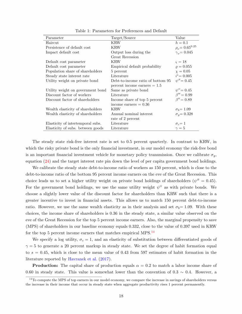
Table 1: Parameters for Preferences and Default

Parameter Target/Source ValueHaircut KRW h = 0.1Persistence of default cost KRW ρν= 0.650.25

Impact default cost Output loss during the γν= 0.045Great Recession

Default cost parameter KRW ς = 18Default cost parameter Empirical default probability % = 0.055Population share of shareholders 5 percent χ = 0.05Steady state interest rate Literature i∗= 0.005Utility weight on private bond Debt-to-income ratio of bottom 95 ψB= 0.45

percent income earners = 1.5Utility weight on government bond Same as private bond ψG= 0.45Discount factor of workers Literature βW = 0.99Discount factor of shareholders Income share of top 5 percent βK= 0.89

income earners = 0.36Wealth elasticity of shareholders KRW σb= 1.09Wealth elasticity of shareholders Annual nominal interest σg= 0.328

rate of 2 percentElasticity of intertemporal subs. Literature σc= 1Elasticity of subs. between goods Literature γ = 5

The steady state risk-free interest rate is set to 0.5 percent quarterly. In contrast to KRW, in

which the risky private bond is the only financial investment, in our model economy the risk-free bond

is an important financial investment vehicle for monetary policy transmission. Once we calibrate σg,

equation (24) and the target interest rate pin down the level of per capita government bond holdings.

We calibrate the steady state debt-to-income ratio of workers as 150 percent, which is close to the

debt-to-income ratio of the bottom 95 percent income earners on the eve of the Great Recession. This

choice leads us to set a higher utility weight on private bond holdings of shareholders (ψB = 0.45).

For the government bond holdings, we use the same utility weight ψG as with private bonds. We

choose a slightly lower value of the discount factor for shareholders than KRW such that there is a

greater incentive to invest in financial assets. This allows us to match 150 percent debt-to-income

ratio. However, we use the same wealth elasticity as in their analysis and set σb= 1.09. With these

choices, the income share of shareholders is 0.36 in the steady state, a similar value observed on the

eve of the Great Recession for the top 5 percent income earners. Also, the marginal propensity to save

(MPS) of shareholders in our baseline economy equals 0.332, close to the value of 0.397 used in KRW

for the top 5 percent income earners that matches empirical MPS.14

We specify a log utility, σc = 1, and an elasticity of substitution between differentiated goods of

γ = 5 to generate a 20 percent markup in steady state. We set the degree of habit formation equal

to s = 0.45, which is close to the mean value of 0.43 from 597 estimates of habit formation in the

literature reported by Havranek et al. (2017).

Production: The capital share of production equals α = 0.2 to match a labor income share of

0.60 in steady state. This value is somewhat lower than the convention of 0.3 ∼ 0.4. However, a

14To compute the MPS of top earners in our model economy, we compare the increase in savings of shareholders versusthe increase in their income that occur in steady state when aggregate productivity rises 1 percent permanently.

18

Table 2: Parameters for Technology, Labor Markets, Nominal Rigidities and Shock Processes

Parameter Target/Source Value

Capital share of production Labor income share = 0.60 α = 0.2Investment adjustment cost Relative volatility of investment κ = 12Habit in consumption Literature s = 0.45Depreciation rate Literature δ = 0.025Separation rate CPS ρ = 0.37Matching efficiency CPS, job finding rate ζ = 0.91Matching function elasticity Literature ε = 0.5Worker’s bargaining power Literature η = 0.5Unemployment benefit bU/w = 0.83 bU= 0.5Vacancy posting cost Literature ξ = 0.11Real wage stickiness S.D. of real comp. 4-quarter growth of ϑ = 50

nonfarm business sector = 1.5 percent

Inflation indexation Literature ε = 0.5Price stickiness S.D. of inflation = 0.64 percent ϕ = 0.935Taylor rule: Inflation gap Literature ρπ= 1.5Persistence of technology shock Literature ρz= 0.85Persistence of bargaining power shock Near Random Walk ρη= 0.90

Persistence of risk premium shock Literature ρφ= 0.85

Std. Dev. of technology shock 1/3 of output variance share and ZLB frequency σz= 0.005Std. Dev. of bargaining power shock 1/3 of output variance share and ZLB frequency ση= 0.0135Std. Dev. of risk premium shock 1/3 of output variance share and ZLB frequency σφ= 0.00075

conventional calibration results in a too-low labor share in our environment given the existence of

rents due to market power, which are divided into different agents according to bargaining power. We

set the coefficient of investment adjustment cost equal to κ = 12 to make investment three times more

volatile than output as in the data. The depreciation rate of capital stock is set to δ = 0.025.

Labor markets: The efficiency of the matching function is set to ζ = 0.91 to hit a quarterly job

finding rate of 85 percent as in the Current Population Survey (CPS). The exogenous gross separation

rate is calibrated to ρ = 0.37, so that the quarterly net separation rate equals 5.6 percent as in the

CPS. For the elasticity of the Cobb-Douglas matching function with respect to vacancies, we follow

the evidence reported in Pissarides and Petrongolo (2001) and set ε = 0.5. We follow much of the

literature and set the steady state workers’ bargaining power to η = 0.5. Unemployment benefits

equal bU = 0.5, which represent 83 percent of the equilibrium wage in steady state. Finally, we set the

vacancy posting cost equal to ξ = 0.11, about 11 percent of labor productivity, essentially the same

as in Hagedorn and Manovskii (2008) and very similar to other values used in the literature.

Price and wage rigidities: We set the real wage adjustment cost parameter ϑ = 50 to match the

standard deviation of the 4-quarter growth rate of real compensation in the non-farm business sector.

Regarding the degree of nominal rigidities, we choose a low value for the probability of resetting the

price (1−ϕ = 0.065) to be consistent with so-called flat Phillips curve. For the same reason, we select

a substantial degree of price indexation (ε = 0.5). With these choices, together with the calibration of

real wage rigidity, inflation in the baseline economy is as volatile as PCE price inflation in the post-war

19

period.

Monetary policy rule: As mentioned earlier, we let the monetary policy rule react only to the

inflation gap given that the nature of the shocks considered are consistent with the so-called divine

coincidence. In the baseline calibration, the inflation coefficient is set to ρπ = 1.5 following Taylor

(1999). Note that in an economy with the divine coincidence, this parametrization without the reaction

term for the output gap implies a more lenient monetary policy rule than in Taylor (1999). However,

we study a range of values for ρπ in our analysis.

Exogenous shock processes: The persistence parameters of the technology shock and the risk

premium shock are chosen to be the same and equal to ρz= ρφ = 0.85. We set the persistence of the

bargaining power shock to a slightly higher value of ρη = 0.9. The reason is that we view changes

in bargaining power as a slow-moving process representing changes in social norms and labor market

institutions. We choose the volatility of the three exogenous shocks such that they have equal variance

decomposition shares for output in the long run, without considering financial crises or ZLB constraint.

This gives us two restrictions. The third ones comes from matching the frequency of being at the ZLB

of around 5 percent, as in Coibion et al. (2012). These three restrictions determine the values for σz,

σφ, and ση. Note that we use the monetary policy shock only to satisfy the ZLB constraint. Overall

the volatility of the cyclical component of output in the baseline economy with financial crises and the

ZLB constraint is 2.2 percent, slightly above the 1.6 percent observed in the United States during the

post-war period.

5 Model Dynamics

This section characterizes the dynamics of the model using impulse response functions. In doing so,

we first assume that neither default nor a binding ZLB constraint occur. We then show how these two

sources of nonlinearity modify model dynamics.

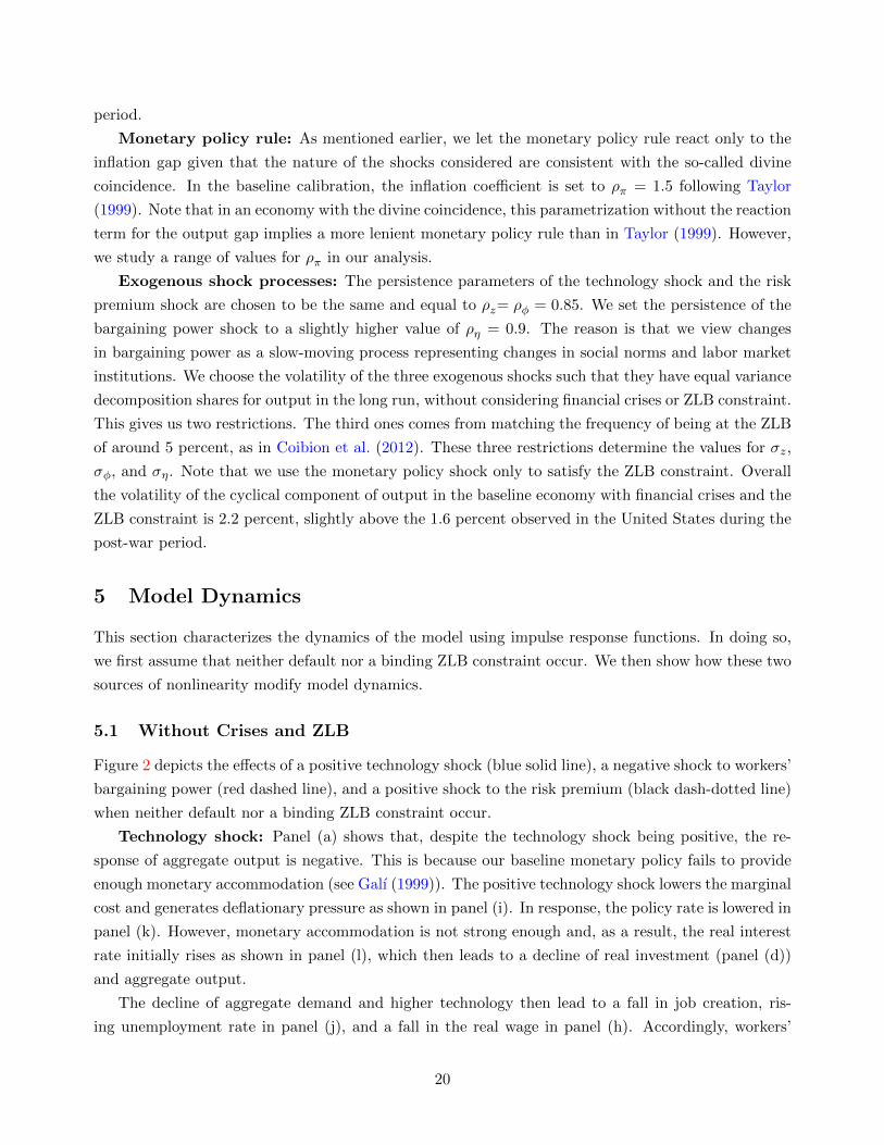
5.1 Without Crises and ZLB

Figure 2 depicts the effects of a positive technology shock (blue solid line), a negative shock to workers’

bargaining power (red dashed line), and a positive shock to the risk premium (black dash-dotted line)

when neither default nor a binding ZLB constraint occur.

Technology shock: Panel (a) shows that, despite the technology shock being positive, the re-

sponse of aggregate output is negative. This is because our baseline monetary policy fails to provide

enough monetary accommodation (see Galı (1999)). The positive technology shock lowers the marginal

cost and generates deflationary pressure as shown in panel (i). In response, the policy rate is lowered in

panel (k). However, monetary accommodation is not strong enough and, as a result, the real interest

rate initially rises as shown in panel (l), which then leads to a decline of real investment (panel (d))

and aggregate output.

The decline of aggregate demand and higher technology then lead to a fall in job creation, ris-

ing unemployment rate in panel (j), and a fall in the real wage in panel (h). Accordingly, workers’

20

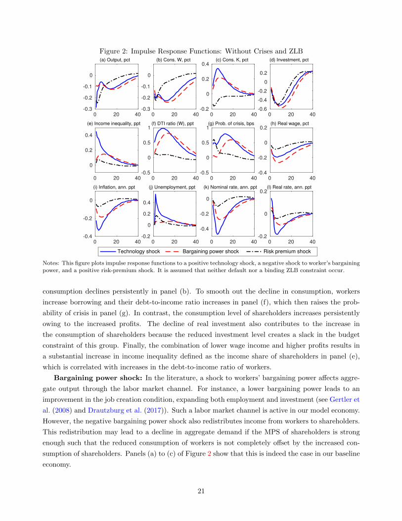
Figure 2: Impulse Response Functions: Without Crises and ZLB

0 20 40-0.3

-0.2

-0.1

0

(a) Output, pct

0 20 40-0.3

-0.2

-0.1

0

(b) Cons. W, pct

0 20 40-0.2

0

0.2

0.4(c) Cons. K, pct

0 20 40-0.6

-0.4

-0.2

0

0.2

(d) Investment, pct

0 20 40

0

0.2

0.4

(e) Income inequality, ppt

0 20 40-0.5

0

0.5

1(f) DTI ratio (W), ppt

0 20 40-0.5

0

0.5

1(g) Prob. of crisis, bps

0 20 40-0.4

-0.2

0

0.2(h) Real wage, pct

0 20 40-0.4

-0.2

0

(i) Inflation, ann. ppt

0 20 40-0.2

0

0.2

0.4

(j) Unemployment, ppt

0 20 40

-0.4

-0.2

0

(k) Nominal rate, ann. ppt

0 20 40-0.2

0

0.2(l) Real rate, ann. ppt

Technology shock Bargaining power shock Risk premium shock

Notes: This figure plots impulse response functions to a positive technology shock, a negative shock to worker’s bargainingpower, and a positive risk-premium shock. It is assumed that neither default nor a binding ZLB constraint occur.

consumption declines persistently in panel (b). To smooth out the decline in consumption, workers

increase borrowing and their debt-to-income ratio increases in panel (f), which then raises the prob-

ability of crisis in panel (g). In contrast, the consumption level of shareholders increases persistently

owing to the increased profits. The decline of real investment also contributes to the increase in

the consumption of shareholders because the reduced investment level creates a slack in the budget

constraint of this group. Finally, the combination of lower wage income and higher profits results in

a substantial increase in income inequality defined as the income share of shareholders in panel (e),

which is correlated with increases in the debt-to-income ratio of workers.

Bargaining power shock: In the literature, a shock to workers’ bargaining power affects aggre-

gate output through the labor market channel. For instance, a lower bargaining power leads to an

improvement in the job creation condition, expanding both employment and investment (see Gertler et

al. (2008) and Drautzburg et al. (2017)). Such a labor market channel is active in our model economy.

However, the negative bargaining power shock also redistributes income from workers to shareholders.

This redistribution may lead to a decline in aggregate demand if the MPS of shareholders is strong

enough such that the reduced consumption of workers is not completely offset by the increased con-

sumption of shareholders. Panels (a) to (c) of Figure 2 show that this is indeed the case in our baseline

economy.

21

Despite the fundamental improvement in the job creation condition, employment actually decreases

because of the fall in aggregate demand. For the same reason, investment decreases. Since lower

bargaining power reduces the real wage persistently, marginal cost declines and the economy faces a

mild deflation pressure.15 Monetary policy reacts by lowering the nominal interest rate, but the real

interest rate is slightly increased. Workers try to smooth out the decline in consumption by issuing

more bonds. Since shareholders have to increase lending, they do not increase consumption sufficiently.

The rise in income inequality generated by the negative bargaining power shock correlates with

the increase in the debt-to-income ratio of workers. As the debt-to-income ratio goes up persistently,

the probability of default rises.

Risk premium shock: Panel (a) of Figure 2 shows that the risk premium shock leads to a

persistent decline in aggregate output. This is driven by the decline in the consumption of shareholders

through the consumption Euler equation and the decline in investment through the investment Euler

equation. While this shock does not directly affect workers’ consumption through their consumption

Euler equation, the shock also leads to a decline in their consumption because the decline of aggregate

demand leads to higher unemployment and lower wages. The debt issuance of workers declines as the

borrowing cost is elevated by this shock. The decline of income and consumption in the context of

higher borrowing cost increases the incentive to default and the default probability goes up, but not

substantially since the borrowers undergo deleveraging in response to the risk-premium shock.

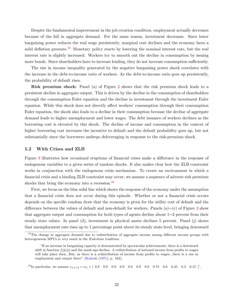
5.2 With Crises and ZLB

Figure 3 illustrates how occasional eruptions of financial crises make a difference in the response of

endogenous variables to a given series of random shocks. It also makes clear how the ZLB constraint

works in conjunction with the endogenous crisis mechanism. To create an environment in which a

financial crisis and a binding ZLB constraint may occur, we assume a sequence of adverse risk premium

shocks that bring the economy into a recession.16

First, we focus on the blue solid line which shows the response of the economy under the assumption

that a financial crisis does not occur during this episode. Whether or not a financial crisis occurs

depends on the specific random draw that the economy is given for the utility cost of default and the

difference between the values of default and non-default for workers. Panels (a)∼(c) of Figure 3 show

that aggregate output and consumption for both types of agents decline about 1∼2 percent from their

steady state values. In panel (d), investment in physical assets declines 5 percent. Panel (j) shows

that unemployment rate rises up to 1 percentage point above its steady state level, bringing downward

15The change in aggregate demand due to redistribution of aggregate income among different income groups withheterogeneous MPCs is very much in the Kaleckian tradition:

“If an increase in bargaining capacity is demonstrated by spectacular achievements, there is a downwardshift in function f(p/p) and the mark-ups decline. A redistribution of national income from profits to wageswill take place then...But, as there is a redistribution of income from profits to wages...there is a rise inemployment and output there”–(Kalecki (1971), p. 162).

16In particular, we assume εφ,1:12 = σφ × [ 0.9 0.9 0.9 0.9 0.9 0.9 0.9 0.75 0.6 0.45 0.3 0.15 ]′.

22

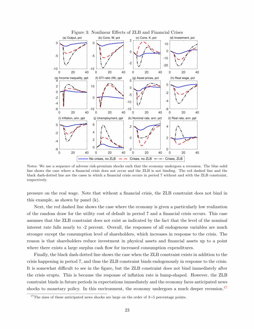
Figure 3: Nonlinear Effects of ZLB and Financial Crises

0 20 40-10

-5

0

(a) Output, pct

0 20 40-10

-5

0

(b) Cons. W, pct

0 20 40

-2

0

2(c) Cons. K, pct

0 20 40

-20

-10

0

10

(d) Investment, pct

0 20 40-6

-4

-2

0

2

4(e) Income inequality, ppt

0 20 40-10

0

10

(f) DTI ratio (W), ppt

0 20 40-15

-10

-5

0

5(g) Asset prices, pct

0 20 40-6

-4

-2

0

(h) Real wage, pct

0 20 40-6

-4

-2

0

(i) Inflation, ann. ppt

0 20 40

0

2

4

6

(j) Unemployment, ppt

0 20 40-2

0

2

(k) Nominal rate, ann. pct

0 20 400

2

4

(l) Real rate, ann. ppt

No crises, no ZLB Crises, no ZLB Crises, ZLB

Notes: We use a sequence of adverse risk-premium shocks such that the economy undergoes a recession. The blue solidline shows the case where a financial crisis does not occur and the ZLB is not binding. The red dashed line and theblack dash-dotted line are the cases in which a financial crisis occurs in period 7 without and with the ZLB constraint,respectively.

pressure on the real wage. Note that without a financial crisis, the ZLB constraint does not bind in

this example, as shown by panel (k).

Next, the red dashed line shows the case where the economy is given a particularly low realization

of the random draw for the utility cost of default in period 7 and a financial crisis occurs. This case

assumes that the ZLB constraint does not exist as indicated by the fact that the level of the nominal

interest rate falls nearly to -2 percent. Overall, the responses of all endogenous variables are much

stronger except the consumption level of shareholders, which increases in response to the crisis. The

reason is that shareholders reduce investment in physical assets and financial assets up to a point

where there exists a large surplus cash flow for increased consumption expenditures.

Finally, the black dash-dotted line shows the case when the ZLB constraint exists in addition to the

crisis happening in period 7, and thus the ZLB constraint binds endogenously in response to the crisis.

It is somewhat difficult to see in the figure, but the ZLB constraint does not bind immediately after

the crisis erupts. This is because the response of inflation rate is hump-shaped. However, the ZLB

constraint binds in future periods in expectations immediately and the economy faces anticipated news

shocks to monetary policy. In this environment, the economy undergoes a much deeper recession.17

17The sizes of these anticipated news shocks are large on the order of 3∼5 percentage points.

23

Aggregate output, for instance, can deviate as much as 6 percentage points from the case without

the crisis and the binding ZLB constraint. In the presence of binding ZLB constraint, the size of the

financial crisis roughly doubles in terms of output loss, unemployment increase and deflation.18

6 Simulation Results: Income Inequality, Aggregate Demand, and

Financial Crises

In this section, we first perform a thought experiment to highlight the link between income inequality

and aggregate demand in the model. We then use stochastic simulations to analyze the key properties

of the model economy.

6.1 Illustration of the Link between Income Inequality and Aggregate Demand

Before describing the main results of the paper, we illustrate the key mechanism that provides links

between income inequality, insufficient aggregate demand and deflation pressure. The fundamental

reason why increases in income inequality lead to insufficient aggregate demand in the model is the

composition of aggregate MPC: Shareholders have a strictly lower MPC than workers due to the

Weberian preferences of “the spirit of capitalism” of shareholders. In this situation, the redistribution

of national income towards workers leads to increases in aggregate demand.

To build intuition, as Keynes (1936) did, let us assume that consumption is a linear function of

income for each agent, where each agent’s income is given by fractions α and 1 − α of aggregate

income y : cW = kWαy and cK = kK(1− α)y with 0 < kK < kW ≤ 1. Consider a simplified version of

aggregate income identity with no adjustment cost: y = cW +cK+x. For now we treat x “autonomous”

component of aggregate demand. Combining the consumption functions and aggregate income identity

yields

y(α) =x

1− [αkW + (1− α)kK ]≡ x

1− k(α)

where 1/(1− k(α)) is our version of what Keynes called “investment multiplier”. Now consider a new

income redistribution α′ > α that increases the share of the income that accrues to the agent with the

highest MPC. It is then clear that

y(α′) =x

1− k(α′)>

x

1− k(α)= y(α),

18Note that the binding ZLB constraint can be thought of as contractionary monetary policy shocks executed by naturerather than by the monetary authority. The difference between the black dash-dotted lines and the red dashed lines inpanels (b) and (c) of Figure 3 show that the monetary policy transmission channel is starkly different for workers andshareholders for the same reason mentioned as for the effects of the risk premium shock. In the case of shareholders,the difference is mainly driven by the intertemporal substitution effect owing to the higher real interest rate during thebinding ZLB episode. In contrast, the reduction in workers’ consumption is primarily driven by the general equilibriumeffects of reduced job creation. While our model is a very stylized, two-agent general equilibrium model, this differencein monetary transmission channels between shareholders and workers is essentially identical to that obtained in the muchricher model of Kaplan et al. (2018), with heterogeneous agents and incomplete markets with multiple assets of differentliquidities.

24

since k(α′) = α′kW + (1 − α′)kK > αkW + (1 − α)kK = k(α). For a given level of autonomous

investment spending x, the ratio y(α′)/y(α) > 1 because [1− k(α)]/[1− k(α′)] > 1, which is the ratio

of the marginal propensities to save in the two economies. This is what we call inequality multiplier.

Note that the size of the inequality multiplier will be greater than y(α′)/y(α) if investment responds

positively to the increase in aggregate demand, i.e., x = xa + βy(α), β > 0 such that

y(α) =xa

1− k(α)− β,

where xa is the autonomous component of investment and 1/[1−k(α)−β] is our version of what Hicks

(1972) called “super-multiplier”. It can be shown that the inequality multiplier can be much greater

if constructed with the super-multiplier.

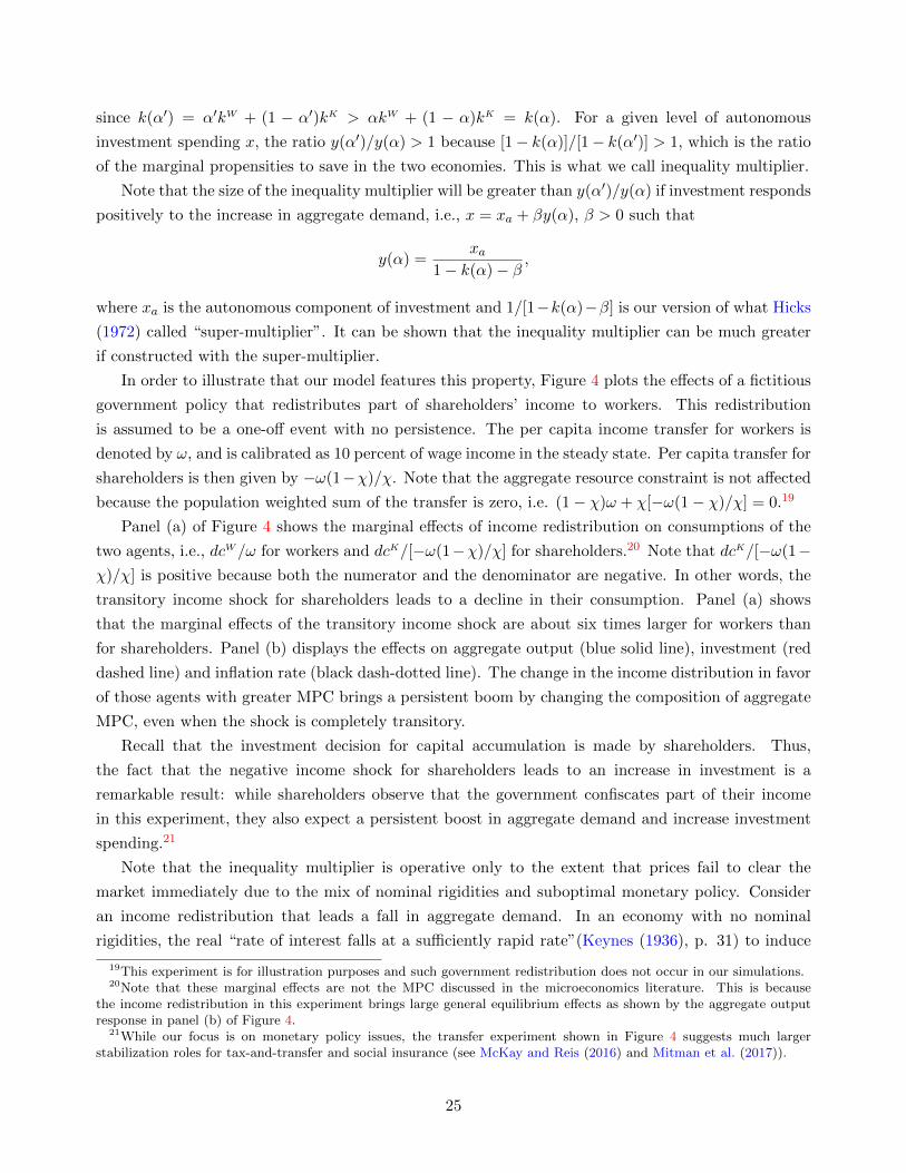
In order to illustrate that our model features this property, Figure 4 plots the effects of a fictitious

government policy that redistributes part of shareholders’ income to workers. This redistribution

is assumed to be a one-off event with no persistence. The per capita income transfer for workers is

denoted by ω, and is calibrated as 10 percent of wage income in the steady state. Per capita transfer for

shareholders is then given by −ω(1−χ)/χ. Note that the aggregate resource constraint is not affected

because the population weighted sum of the transfer is zero, i.e. (1− χ)ω + χ[−ω(1− χ)/χ] = 0.19

Panel (a) of Figure 4 shows the marginal effects of income redistribution on consumptions of the

two agents, i.e., dcW/ω for workers and dcK/[−ω(1−χ)/χ] for shareholders.20 Note that dcK/[−ω(1−χ)/χ] is positive because both the numerator and the denominator are negative. In other words, the

transitory income shock for shareholders leads to a decline in their consumption. Panel (a) shows

that the marginal effects of the transitory income shock are about six times larger for workers than

for shareholders. Panel (b) displays the effects on aggregate output (blue solid line), investment (red

dashed line) and inflation rate (black dash-dotted line). The change in the income distribution in favor

of those agents with greater MPC brings a persistent boom by changing the composition of aggregate

MPC, even when the shock is completely transitory.

Recall that the investment decision for capital accumulation is made by shareholders. Thus,

the fact that the negative income shock for shareholders leads to an increase in investment is a

remarkable result: while shareholders observe that the government confiscates part of their income

in this experiment, they also expect a persistent boost in aggregate demand and increase investment

spending.21

Note that the inequality multiplier is operative only to the extent that prices fail to clear the

market immediately due to the mix of nominal rigidities and suboptimal monetary policy. Consider

an income redistribution that leads a fall in aggregate demand. In an economy with no nominal

rigidities, the real “rate of interest falls at a sufficiently rapid rate”(Keynes (1936), p. 31) to induce

19This experiment is for illustration purposes and such government redistribution does not occur in our simulations.20Note that these marginal effects are not the MPC discussed in the microeconomics literature. This is because

the income redistribution in this experiment brings large general equilibrium effects as shown by the aggregate outputresponse in panel (b) of Figure 4.

21While our focus is on monetary policy issues, the transfer experiment shown in Figure 4 suggests much largerstabilization roles for tax-and-transfer and social insurance (see McKay and Reis (2016) and Mitman et al. (2017)).

25

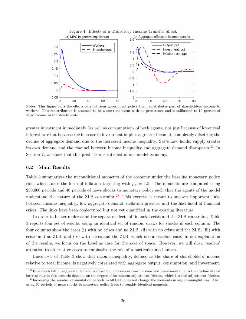
Figure 4: Effects of a Transitory Income Transfer Shock

0 20 40 60 80-0.05

0

0.05

0.1

0.15

0.2

0.25

0.3

(a) MPC in general equilibrium

Workers

Shareholders

0 20 40 60 80-2

-1.5

-1

-0.5

0

0.5

1

1.5

2

2.5(b) Aggregate effects of income transfer

Output, pct

Investment, pct

Inflation, ann.ppt

Notes: This figure plots the effects of a fictitious government policy that redistributes part of shareholders’ income toworkers. This redistribution is assumed to be a one-time event with no persistence and is calibrated to 10 percent ofwage income in the steady state.

greater investment immediately (as well as consumptions of both agents, not just because of lower real

interest rate but because the increase in investment implies a greater income), completely offsetting the

decline of aggregate demand due to the increased income inequality. Say’s Law holds: supply creates

its own demand and the channel between income inequality and aggregate demand disappears.22 In

Section 7, we show that this prediction is satisfied in our model economy.

6.2 Main Results

Table 3 summarizes the unconditional moments of the economy under the baseline monetary policy

rule, which takes the form of inflation targeting with ρπ = 1.5. The moments are computed using

250,000 periods and 40 periods of news shocks to monetary policy such that the agents of the model

understand the nature of the ZLB constraint.23 This exercise is meant to uncover important links

between income inequality, low aggregate demand, deflation pressure and the likelihood of financial

crises. The links have been conjectured but not yet quantified in the existing literature.

In order to better understand the separate effects of financial crisis and the ZLB constraint, Table

3 reports four set of results, using an identical set of random draws for shocks in each column. The

four columns show the cases (i) with no crises and no ZLB, (ii) with no crises and the ZLB, (iii) with

crises and no ZLB, and (iv) with crises and the ZLB, which is our baseline case. In our explanation

of the results, we focus on the baseline case for the sake of space. However, we will draw readers’

attention to alternative cases to emphasize the role of a particular mechanism.

Lines 1∼3 of Table 3 show that income inequality, defined as the share of shareholders’ income

relative to total income, is negatively correlated with aggregate output, consumption, and investment,

22How much fall in aggregate demand is offset by increases in consumption and investment due to the decline of realinterest rate in this scenario depends on the degree of investment adjustment friction, which is a real adjustment friction.

23Increasing the number of simulation periods to 500,000 does not change the moments in any meaningful way. Also,using 60 periods of news shocks to monetary policy leads to roughly identical moments.

26

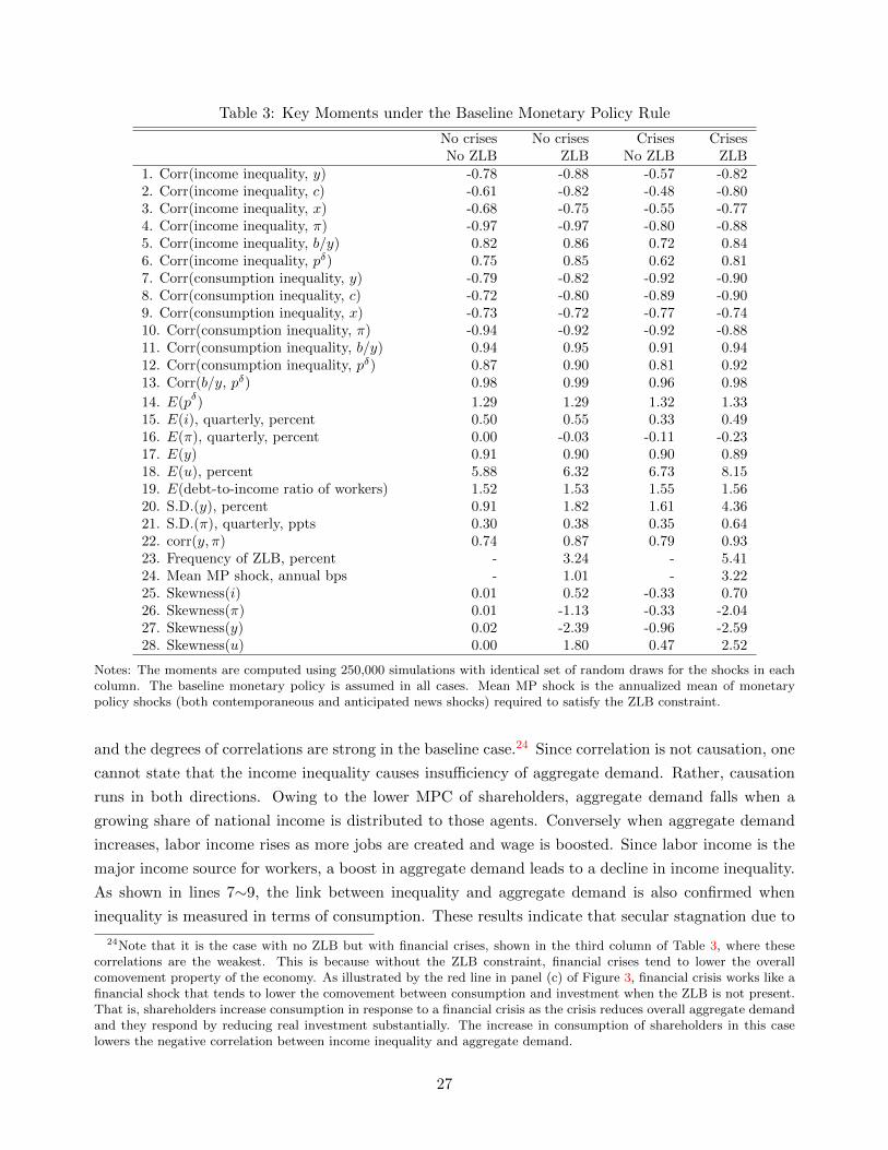
Table 3: Key Moments under the Baseline Monetary Policy Rule

No crises No crises Crises CrisesNo ZLB ZLB No ZLB ZLB

1. Corr(income inequality, y) -0.78 -0.88 -0.57 -0.822. Corr(income inequality, c) -0.61 -0.82 -0.48 -0.803. Corr(income inequality, x) -0.68 -0.75 -0.55 -0.774. Corr(income inequality, π) -0.97 -0.97 -0.80 -0.885. Corr(income inequality, b/y) 0.82 0.86 0.72 0.846. Corr(income inequality, pδ) 0.75 0.85 0.62 0.817. Corr(consumption inequality, y) -0.79 -0.82 -0.92 -0.908. Corr(consumption inequality, c) -0.72 -0.80 -0.89 -0.909. Corr(consumption inequality, x) -0.73 -0.72 -0.77 -0.7410. Corr(consumption inequality, π) -0.94 -0.92 -0.92 -0.8811. Corr(consumption inequality, b/y) 0.94 0.95 0.91 0.9412. Corr(consumption inequality, pδ) 0.87 0.90 0.81 0.9213. Corr(b/y, pδ) 0.98 0.99 0.96 0.98

14. E(pδ) 1.29 1.29 1.32 1.33

15. E(i), quarterly, percent 0.50 0.55 0.33 0.4916. E(π), quarterly, percent 0.00 -0.03 -0.11 -0.2317. E(y) 0.91 0.90 0.90 0.8918. E(u), percent 5.88 6.32 6.73 8.1519. E(debt-to-income ratio of workers) 1.52 1.53 1.55 1.5620. S.D.(y), percent 0.91 1.82 1.61 4.3621. S.D.(π), quarterly, ppts 0.30 0.38 0.35 0.6422. corr(y, π) 0.74 0.87 0.79 0.9323. Frequency of ZLB, percent - 3.24 - 5.4124. Mean MP shock, annual bps - 1.01 - 3.2225. Skewness(i) 0.01 0.52 -0.33 0.7026. Skewness(π) 0.01 -1.13 -0.33 -2.0427. Skewness(y) 0.02 -2.39 -0.96 -2.5928. Skewness(u) 0.00 1.80 0.47 2.52

Notes: The moments are computed using 250,000 simulations with identical set of random draws for the shocks in eachcolumn. The baseline monetary policy is assumed in all cases. Mean MP shock is the annualized mean of monetarypolicy shocks (both contemporaneous and anticipated news shocks) required to satisfy the ZLB constraint.

and the degrees of correlations are strong in the baseline case.24 Since correlation is not causation, one

cannot state that the income inequality causes insufficiency of aggregate demand. Rather, causation

runs in both directions. Owing to the lower MPC of shareholders, aggregate demand falls when a

growing share of national income is distributed to those agents. Conversely when aggregate demand

increases, labor income rises as more jobs are created and wage is boosted. Since labor income is the

major income source for workers, a boost in aggregate demand leads to a decline in income inequality.

As shown in lines 7∼9, the link between inequality and aggregate demand is also confirmed when

inequality is measured in terms of consumption. These results indicate that secular stagnation due to

24Note that it is the case with no ZLB but with financial crises, shown in the third column of Table 3, where thesecorrelations are the weakest. This is because without the ZLB constraint, financial crises tend to lower the overallcomovement property of the economy. As illustrated by the red line in panel (c) of Figure 3, financial crisis works like afinancial shock that tends to lower the comovement between consumption and investment when the ZLB is not present.That is, shareholders increase consumption in response to a financial crisis as the crisis reduces overall aggregate demandand they respond by reducing real investment substantially. The increase in consumption of shareholders in this caselowers the negative correlation between income inequality and aggregate demand.

27

income inequality and underconsumption, originally raised by Hansen (1939) and recently re-taken by

Summers (2015), can be a real possibility.

Line 4 of Table 3 shows a strong, negative correlation between income inequality and the inflation

rate. Again, causation runs in both direction. Since income inequality is negatively correlated with

aggregate demand, it is also negatively correlated with inflation. Conversely, deflation elevates the

real debt burden of workers and redistributes income towards shareholders, increasing the degree of

income inequality. We want to emphasize the role played by nominal rigidities. Without them, a

negative correlation between income inequality and aggregate demand cannot exist in KRW’s original

framework as Say’s Law holds regardless of the degree of income inequality.

Lines 5 and 11 of Table 3 show that the strong correlation between income/consumption inequality

and excess credit, defined as the deviations of credit-to-GDP ratio from its steady state, such as seen in

the data, can be replicated by our model. More importantly, lines 6 and 12 indicate a strong correlation

between inequality and the probability of financial crises. This arises due to the near perfect linear

relationship between excess credit and the probability of financial crises regardless of the presence of

the ZLB constraint, as shown in line 13. Such a linear relationship replicates the empirical findings

by Jorda et al. (2011) and Schularick and Taylor (2012).25

Interestingly, the tie between income inequality and aggregate demand is much stronger in the

presence of the ZLB constraint.26 This indicates that a failure to provide a sufficient degree of monetary

accommodation during economic downturns strengthens the nexus between income inequality and

aggregate demand. The presence of the ZLB constraint also slightly increases the probability of

financial crises, due to slightly higher debt-to-income ratio of workers.

Importantly, both financial crises and the presence of the ZLB constraint modify the distributions

of equilibrium quantities and prices. In particular, with no financial crises and no ZLB constraint (first

column of Table 3), the skewness of endogenous variables (see lines 26∼28) is basically zero, which

should not be surprising given the assumed Gaussian shocks. This also implies that the mean of their

distributions coincides with the non-stochastic steady state of each variable (see lines 16∼18). When

financial crises are included but not the ZLB constraint (third column), the distributions of inflation,

aggregate output and unemployment rate become skewed to the downside and their means deviate

from the non-stochastic steady state values. Thus, financial crises create skewness to the distributions.

The combination of crises and the ZLB constraint (fourth column) creates extraordinary degrees of

skewness for the endogenous variables. Since negative skewness assigns more probability mass to the

downside of the economy, the mean levels of the inflation rate and aggregate output are substantially

lower. Indeed, the presence of the ZLB constraint doubles the deflation bias created by financial crises

and lowers the mean level of output by 1 percent.27 Figure 5 shows how the exact shapes of the

25The linear relationship also justifies the reduced form approach that assumes a (log) linear relationship betweenthe excess credit and the probability of disaster without structural modeling, an approach recently taken by Gourio etal. (2018). In Appendix D, using our simulated data, we replicate the results of Paul (2017) that income inequalitydominates credit in the predictive power of financial crises.

26Figure 11 in Appendix D shows the unconditional and conditional means of monetary policy shocks (both contem-poraneous and anticipated news shocks) needed to satisfy the ZLB constraint in the baseline economy.

27Note that the skewness of the unemployment rate without the ZLB constraint is 0.47 in our economy, which is the

28

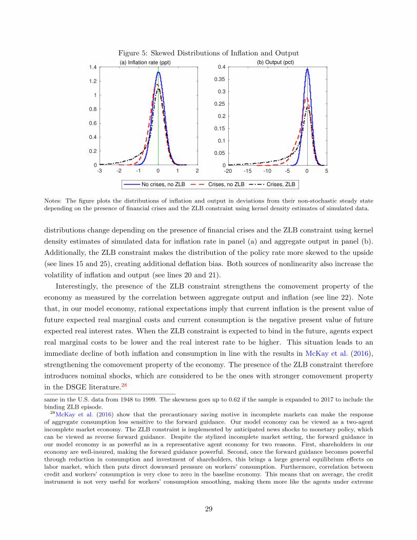
Figure 5: Skewed Distributions of Inflation and Output

-3 -2 -1 0 1 20

0.2

0.4

0.6

0.8

1

1.2

1.4(a) Inflation rate (ppt)

-20 -15 -10 -5 0 50

0.05

0.1

0.15

0.2

0.25

0.3

0.35

0.4(b) Output (pct)

No crises, no ZLB Crises, no ZLB Crises, ZLB

Notes: The figure plots the distributions of inflation and output in deviations from their non-stochastic steady statedepending on the presence of financial crises and the ZLB constraint using kernel density estimates of simulated data.

distributions change depending on the presence of financial crises and the ZLB constraint using kernel

density estimates of simulated data for inflation rate in panel (a) and aggregate output in panel (b).

Additionally, the ZLB constraint makes the distribution of the policy rate more skewed to the upside

(see lines 15 and 25), creating additional deflation bias. Both sources of nonlinearity also increase the

volatility of inflation and output (see lines 20 and 21).

Interestingly, the presence of the ZLB constraint strengthens the comovement property of the

economy as measured by the correlation between aggregate output and inflation (see line 22). Note

that, in our model economy, rational expectations imply that current inflation is the present value of

future expected real marginal costs and current consumption is the negative present value of future

expected real interest rates. When the ZLB constraint is expected to bind in the future, agents expect

real marginal costs to be lower and the real interest rate to be higher. This situation leads to an

immediate decline of both inflation and consumption in line with the results in McKay et al. (2016),

strengthening the comovement property of the economy. The presence of the ZLB constraint therefore

introduces nominal shocks, which are considered to be the ones with stronger comovement property

in the DSGE literature.28

same in the U.S. data from 1948 to 1999. The skewness goes up to 0.62 if the sample is expanded to 2017 to include thebinding ZLB episode.

28McKay et al. (2016) show that the precautionary saving motive in incomplete markets can make the responseof aggregate consumption less sensitive to the forward guidance. Our model economy can be viewed as a two-agentincomplete market economy. The ZLB constraint is implemented by anticipated news shocks to monetary policy, whichcan be viewed as reverse forward guidance. Despite the stylized incomplete market setting, the forward guidance inour model economy is as powerful as in a representative agent economy for two reasons. First, shareholders in oureconomy are well-insured, making the forward guidance powerful. Second, once the forward guidance becomes powerfulthrough reduction in consumption and investment of shareholders, this brings a large general equilibrium effects onlabor market, which then puts direct downward pressure on workers’ consumption. Furthermore, correlation betweencredit and workers’ consumption is very close to zero in the baseline economy. This means that on average, the creditinstrument is not very useful for workers’ consumption smoothing, making them more like the agents under extreme

29

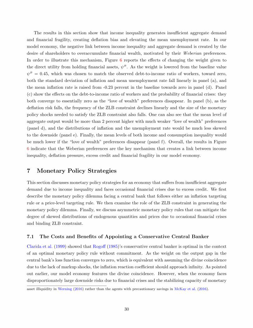
The results in this section show that income inequality generates insufficient aggregate demand

and financial fragility, creating deflation bias and elevating the mean unemployment rate. In our

model economy, the negative link between income inequality and aggregate demand is created by the

desire of shareholders to overaccumulate financial wealth, motivated by their Weberian preferences.

In order to illustrate this mechanism, Figure 6 reports the effects of changing the weight given to

the direct utility from holding financial assets, ψB. As the weight is lowered from the baseline value

ψB = 0.45, which was chosen to match the observed debt-to-income ratio of workers, toward zero,

both the standard deviation of inflation and mean unemployment rate fall linearly in panel (a), and

the mean inflation rate is raised from -0.23 percent in the baseline towards zero in panel (d). Panel

(c) show the effects on the debt-to-income ratio of workers and the probability of financial crises: they

both converge to essentially zero as the “love of wealth” preferences disappear. In panel (b), as the

deflation risk falls, the frequency of the ZLB constraint declines linearly and the size of the monetary

policy shocks needed to satisfy the ZLB constraint also falls. One can also see that the mean level of

aggregate output would be more than 2 percent higher with much weaker “love of wealth” preferences

(panel d), and the distributions of inflation and the unemployment rate would be much less skewed

to the downside (panel e). Finally, the mean levels of both income and consumption inequality would

be much lower if the “love of wealth” preferences disappear (panel f). Overall, the results in Figure

6 indicate that the Weberian preferences are the key mechanism that creates a link between income

inequality, deflation pressure, excess credit and financial fragility in our model economy.

7 Monetary Policy Strategies

This section discusses monetary policy strategies for an economy that suffers from insufficient aggregate

demand due to income inequality and faces occasional financial crises due to excess credit. We first

describe the monetary policy dilemma facing a central bank that follows either an inflation targeting

rule or a price-level targeting rule. We then examine the role of the ZLB constraint in generating the

monetary policy dilemma. Finally, we discuss asymmetric monetary policy rules that can mitigate the

degree of skewed distributions of endogenous quantities and prices due to occasional financial crises

and binding ZLB constraint.

7.1 The Costs and Benefits of Appointing a Conservative Central Banker

Clarida et al. (1999) showed that Rogoff (1985)’s conservative central banker is optimal in the context

of an optimal monetary policy rule without commitment. As the weight on the output gap in the

central bank’s loss function converges to zero, which is equivalent with assuming the divine coincidence

due to the lack of markup shocks, the inflation reaction coefficient should approach infinity. As pointed

out earlier, our model economy features the divine coincidence. However, when the economy faces

disproportionately large downside risks due to financial crises and the stabilizing capacity of monetary

asset illiquidity in Werning (2016) rather than the agents with precautionary savings in McKay et al. (2016).

30

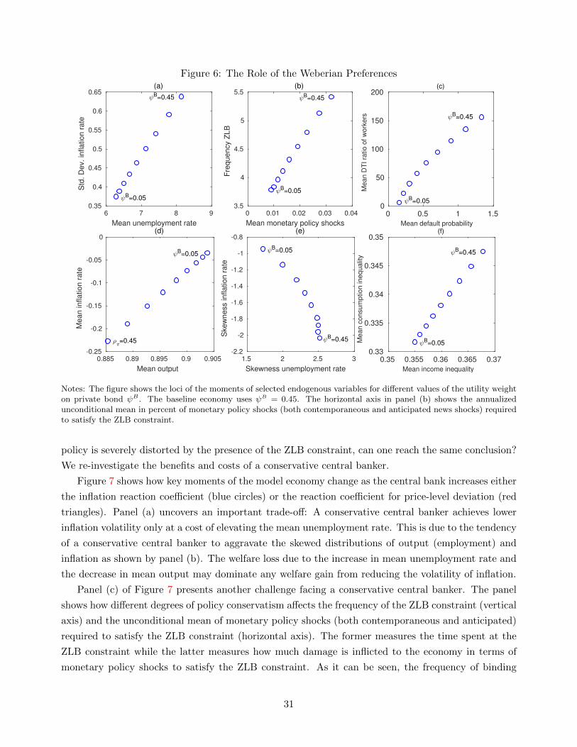
Figure 6: The Role of the Weberian Preferences

6 7 8 9

Mean unemployment rate

0.35

0.4

0.45

0.5

0.55

0.6

0.65

Std

. D

ev.

infla

tio

n r

ate

(a)

B=0.05

B=0.45

0 0.01 0.02 0.03 0.04

Mean monetary policy shocks

3.5

4

4.5

5

5.5

Fre

qu

en

cy Z

LB

(b)

B=0.05

B=0.45

0 0.5 1 1.5

Mean default probability

0

50

100

150

200

Me

an

DT

I ra

tio

of

wo

rke

rs

(c)

B=0.05

B=0.45

0.885 0.89 0.895 0.9 0.905

Mean output

-0.25

-0.2

-0.15

-0.1

-0.05

0

Me

an

in

fla

tio

n r

ate

(d)

B=0.05

=0.45

1.5 2 2.5 3

Skewness unemployment rate

-2.2

-2

-1.8

-1.6

-1.4

-1.2

-1

-0.8

Ske

wn

ess in

fla

tio

n r

ate

(e)

B=0.05

B=0.45

0.35 0.355 0.36 0.365 0.37

Mean income inequality

0.33

0.335

0.34

0.345

0.35

Me

an

co

nsu

mp

tio

n in

eq

ua

lity

(f)

B=0.05

B=0.45

Notes: The figure shows the loci of the moments of selected endogenous variables for different values of the utility weighton private bond ψB . The baseline economy uses ψB = 0.45. The horizontal axis in panel (b) shows the annualizedunconditional mean in percent of monetary policy shocks (both contemporaneous and anticipated news shocks) requiredto satisfy the ZLB constraint.

policy is severely distorted by the presence of the ZLB constraint, can one reach the same conclusion?

We re-investigate the benefits and costs of a conservative central banker.

Figure 7 shows how key moments of the model economy change as the central bank increases either

the inflation reaction coefficient (blue circles) or the reaction coefficient for price-level deviation (red

triangles). Panel (a) uncovers an important trade-off: A conservative central banker achieves lower

inflation volatility only at a cost of elevating the mean unemployment rate. This is due to the tendency

of a conservative central banker to aggravate the skewed distributions of output (employment) and

inflation as shown by panel (b). The welfare loss due to the increase in mean unemployment rate and

the decrease in mean output may dominate any welfare gain from reducing the volatility of inflation.

Panel (c) of Figure 7 presents another challenge facing a conservative central banker. The panel

shows how different degrees of policy conservatism affects the frequency of the ZLB constraint (vertical

axis) and the unconditional mean of monetary policy shocks (both contemporaneous and anticipated)

required to satisfy the ZLB constraint (horizontal axis). The former measures the time spent at the

ZLB constraint while the latter measures how much damage is inflicted to the economy in terms of

monetary policy shocks to satisfy the ZLB constraint. As it can be seen, the frequency of binding

31

Figure 7: The Consequences of Conservatism in Monetary Policy

6 7 8 9

Mean unemployment rate

0.3

0.4

0.5

0.6

0.7S

td.

De

v.

infla

tio

n r

ate

(a)

=1

=20

=0.1

=4

-4 -3 -2 -1 0

Skewness output

-4

-3

-2

-1

0

Ske

wn

ess in

fla

tio

n r

ate

=20

=1

=0.1

=4

(b)

0 0.5 1 1.5 2

Mean monetary policy shocks

0

2

4

6

8

10

12

Fre

qu

en

cy Z

LB

(c)

=1

=20

=0.1

=4

1.33 1.335 1.34 1.345

Mean default probability

-30

-20

-10

0

10

Cu

mu

lative

ou

tpu

t lo

ss u

po

n c

risis

(d)

=1

=20 =0.1

=4

Inflation targeting Price-level targeting

0.88 0.89 0.9 0.91

Mean output

-0.3

-0.2

-0.1

0

Me

an

in

fla

tio

n r

ate

(e)

=1

=20

=0.1

=4

-1 -0.8 -0.6

Corr(inc. inequality,output)

-0.9

-0.85

-0.8

-0.75

-0.7

-0.65

-0.6

Co

rr(in

c.

ine

qu

alit

y,in

fla

tio

n)

=20

=1

=0.1

=4

(f)

Notes: The figure shows the loci of the moments of selected endogenous variables as the central bank increases eitherthe inflation reaction coefficient ρπ (inflation targeting) or the reaction coefficient for price-level deviation ρΠ (price-leveltargeting). The horizontal axis in panel (c) shows the annualized unconditional mean in percent of monetary policyshocks (both contemporaneous and anticipated news shocks) required to satisfy the ZLB constraint.

ZLB constraint increases monotonically for both inflation targeting and price-level targeting as policy

conservatism is strengthened. Furthermore, the mean level of monetary policy shocks used to satisfy

the ZLB constraint, which can be interpreted as the shadow value of the ZLB constraint, also increases

monotonically with the degree of policy conservatism.

Panel (d) of Figure 7 shows two aspects of policy conservatism regarding the probability of financial

crises (horizontal axis) and the cumulative output loss upon a financial crisis (vertical axis). For both

rules, a conservative central banker tends to increase the probability of financial crises. This is because

strong reactions in monetary policy rates to inflation tends to elevate debt-servicing costs of borrowers.

Furthermore, the increase in unemployment rate due to hawkish monetary policy as shown in panel

(a) also elevates the debt-to-income ratio and thus strengthens the incentive of borrowers to default.

However, the same conservative central banker has a virtue of providing a massive amount of monetary

accommodation during a financial crisis, limiting the size of the cumulative output drop.29

It is notable that while the price-level targeting regime faces the same type of trade-off between

29Figure 12 in Appendix D replicates the experiment shown in Figure 3 when both financial crises and the ZLBconstraint are present for a range of calibrated inflation targeting and price-level targeting rules.

32

stabilization of inflation volatility and reduction of the mean unemployment rate, it substantially

improves the nature of the trade-off. This can be seen in the fact that the frontier associated with the

price-level targeting is located much lower and more to the left in panel (a) of Figure 7. Furthermore,

as shown in panel (b), the absolute degrees of skewness of the distributions are also much smaller with

the price-level targeting as compared with the inflation targeting.

Price-level targeting can also be much more effective in controlling the deflation bias. Panel (e)

of Figure 7 shows the mean inflation rate on the vertical axis and the mean aggregate output on the

horizontal axis. The results suggest that, in contrast to the inflation targeting, price-level targeting

eliminates the deflation bias almost completely regardless of the degree of the conservatism of monetary

policymakers. It also suggests that simply switching from the inflation targeting with ρπ = 20 to the

price-level targeting with ρΠ = 0.1 can result in an almost 3 percent increase in the mean level of

aggregate output, which has significant implications for the welfare of both types of agents.30 Panel

(e) also suggests that, if the price-level targeting cannot be implemented, adopting the most lenient

inflation targeting regime can minimize the deflation bias at the cost of increased inflation volatility.

Finally, panel (f) of Figure 7 shows how monetary policy conservatism affects the correlation

between income inequality and the inflation rate (vertical axis) and the correlation between income

inequality and output (horizontal axis). The results point out that price-level targeting can be much

more effective in breaking the link between income inequality and aggregate demand in the model. In

fact, no level of inflation targeting is nearly as successful as the price-level targeting in breaking the

tie between income inequality and aggregate demand.

Summing up, the investigation of various aspects of the economy under alternative monetary

policy rules leads to two conclusions regarding the desirability of monetary policy conservatism. First,

regardless of optimality of a conservative central banker, price-level targeting outperforms inflation

targeting in many dimensions such as containing the deflation bias created by occasional financial

crises and binding ZLB constraint. Second, conservatism in monetary policy may lead to greater

deflation bias and more frequent financial crises in an economy suffering from insufficient aggregate

demand due to income inequality, though the same conservatism may have a benefit of providing a

protection against downside risk conditioned upon an actual financial crisis. The second conclusion

seems to suggest that in an economy in which an active link exists among income inequality, deflation

pressure and financial crises, a mix of a dovish central banker and extraordinary stabilization measures

that are implemented only during financial crises may improve upon symmetric monetary policy rules.

7.2 The Role of the ZLB Constraint

Before we move onto the analysis of optimal monetary policy, we want to emphasize that the trade-off

facing a conservative central banker is due to the presence of the ZLB constraint. In other words,

the presence of occasional financial crises alone does not create the trade-off in monetary policy. To

30Output loss associated with appointing a conservative central bank has two sources: skewed distributions of produc-tion inputs and price dispersion due to the deflation bias. The latter does not exist for price-level targeting regardless ofpolicy conservatism as the rule eliminates the bias almost completely.

33

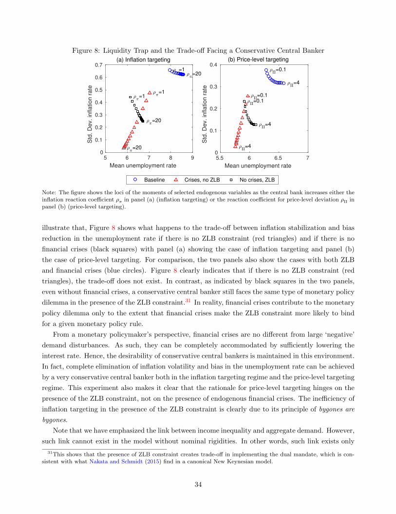
Figure 8: Liquidity Trap and the Trade-off Facing a Conservative Central Banker

5 6 7 8 9

Mean unemployment rate

0

0.1

0.2

0.3

0.4

0.5

0.6

0.7

Std

. D

ev. in

flation r

ate

(a) Inflation targeting

=1 =20

=1

=20

=1

=20

5.5 6 6.5 7

Mean unemployment rate

0

0.1

0.2

0.3

0.4

Std

. D

ev. in

flation r

ate

(b) Price-level targeting

=0.1

=4

=0.1

=4

=0.1

=4

Baseline Crises, no ZLB No crises, ZLB

Note: The figure shows the loci of the moments of selected endogenous variables as the central bank increases either theinflation reaction coefficient ρπ in panel (a) (inflation targeting) or the reaction coefficient for price-level deviation ρΠ inpanel (b) (price-level targeting).

illustrate that, Figure 8 shows what happens to the trade-off between inflation stabilization and bias

reduction in the unemployment rate if there is no ZLB constraint (red triangles) and if there is no

financial crises (black squares) with panel (a) showing the case of inflation targeting and panel (b)

the case of price-level targeting. For comparison, the two panels also show the cases with both ZLB

and financial crises (blue circles). Figure 8 clearly indicates that if there is no ZLB constraint (red

triangles), the trade-off does not exist. In contrast, as indicated by black squares in the two panels,

even without financial crises, a conservative central banker still faces the same type of monetary policy

dilemma in the presence of the ZLB constraint.31 In reality, financial crises contribute to the monetary

policy dilemma only to the extent that financial crises make the ZLB constraint more likely to bind

for a given monetary policy rule.

From a monetary policymaker’s perspective, financial crises are no different from large ‘negative’

demand disturbances. As such, they can be completely accommodated by sufficiently lowering the

interest rate. Hence, the desirability of conservative central bankers is maintained in this environment.

In fact, complete elimination of inflation volatility and bias in the unemployment rate can be achieved

by a very conservative central banker both in the inflation targeting regime and the price-level targeting

regime. This experiment also makes it clear that the rationale for price-level targeting hinges on the

presence of the ZLB constraint, not on the presence of endogenous financial crises. The inefficiency of

inflation targeting in the presence of the ZLB constraint is clearly due to its principle of bygones are

bygones.

Note that we have emphasized the link between income inequality and aggregate demand. However,

such link cannot exist in the model without nominal rigidities. In other words, such link exists only

31This shows that the presence of ZLB constraint creates trade-off in implementing the dual mandate, which is con-sistent with what Nakata and Schmidt (2015) find in a canonical New Keynesian model.

34

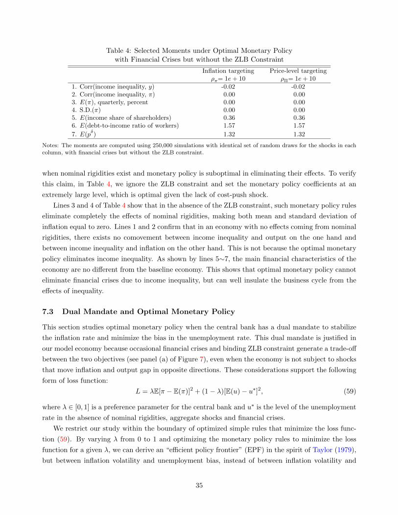
Table 4: Selected Moments under Optimal Monetary Policywith Financial Crises but without the ZLB Constraint

Inflation targeting Price-level targetingρπ= 1e+ 10 ρΠ= 1e+ 10

1. Corr(income inequality, y) -0.02 -0.022. Corr(income inequality, π) 0.00 0.003. E(π), quarterly, percent 0.00 0.004. S.D.(π) 0.00 0.005. E(income share of shareholders) 0.36 0.366. E(debt-to-income ratio of workers) 1.57 1.57

7. E(pδ) 1.32 1.32

Notes: The moments are computed using 250,000 simulations with identical set of random draws for the shocks in eachcolumn, with financial crises but without the ZLB constraint.

when nominal rigidities exist and monetary policy is suboptimal in eliminating their effects. To verify

this claim, in Table 4, we ignore the ZLB constraint and set the monetary policy coefficients at an

extremely large level, which is optimal given the lack of cost-push shock.

Lines 3 and 4 of Table 4 show that in the absence of the ZLB constraint, such monetary policy rules

eliminate completely the effects of nominal rigidities, making both mean and standard deviation of

inflation equal to zero. Lines 1 and 2 confirm that in an economy with no effects coming from nominal

rigidities, there exists no comovement between income inequality and output on the one hand and

between income inequality and inflation on the other hand. This is not because the optimal monetary

policy eliminates income inequality. As shown by lines 5∼7, the main financial characteristics of the

economy are no different from the baseline economy. This shows that optimal monetary policy cannot

eliminate financial crises due to income inequality, but can well insulate the business cycle from the

effects of inequality.

7.3 Dual Mandate and Optimal Monetary Policy

This section studies optimal monetary policy when the central bank has a dual mandate to stabilize

the inflation rate and minimize the bias in the unemployment rate. This dual mandate is justified in

our model economy because occasional financial crises and binding ZLB constraint generate a trade-off

between the two objectives (see panel (a) of Figure 7), even when the economy is not subject to shocks

that move inflation and output gap in opposite directions. These considerations support the following

form of loss function:

L = λE[π − E(π)]2 + (1− λ)[E(u)− u∗]2, (59)

where λ ∈ [0, 1] is a preference parameter for the central bank and u∗ is the level of the unemployment

rate in the absence of nominal rigidities, aggregate shocks and financial crises.

We restrict our study within the boundary of optimized simple rules that minimize the loss func-

tion (59). By varying λ from 0 to 1 and optimizing the monetary policy rules to minimize the loss

function for a given λ, we can derive an “efficient policy frontier” (EPF) in the spirit of Taylor (1979),

but between inflation volatility and unemployment bias, instead of between inflation volatility and

35

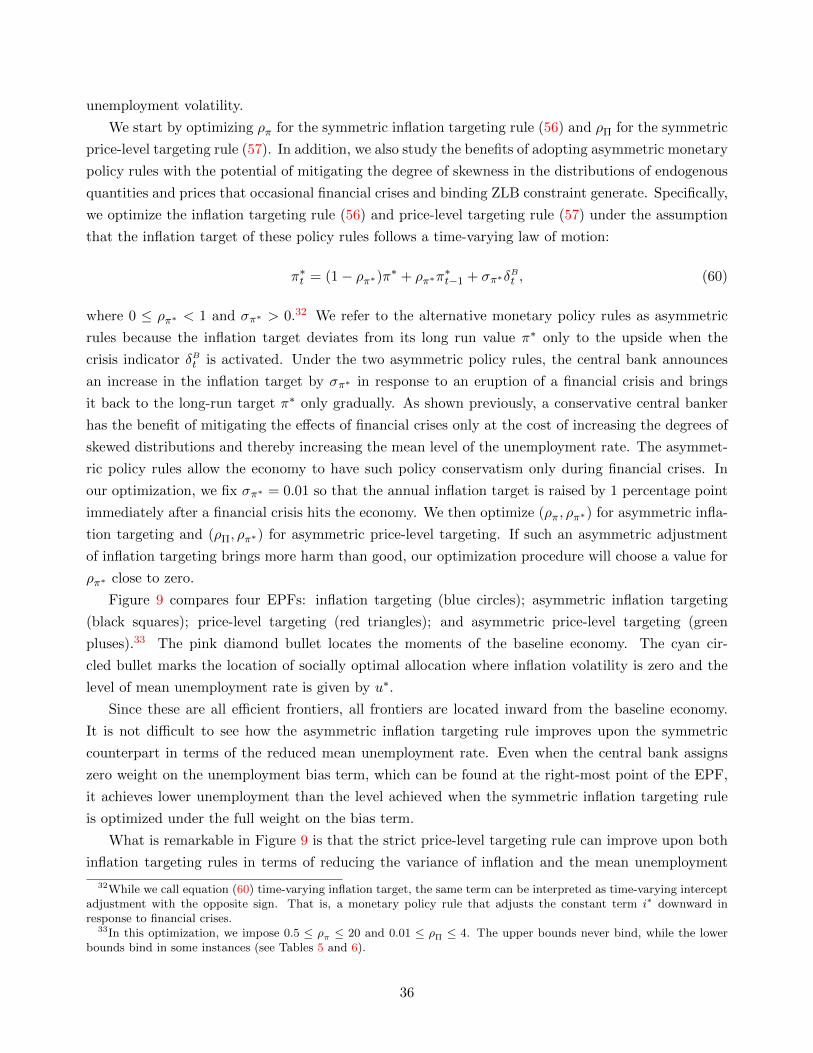
unemployment volatility.

We start by optimizing ρπ for the symmetric inflation targeting rule (56) and ρΠ for the symmetric

price-level targeting rule (57). In addition, we also study the benefits of adopting asymmetric monetary

policy rules with the potential of mitigating the degree of skewness in the distributions of endogenous

quantities and prices that occasional financial crises and binding ZLB constraint generate. Specifically,

we optimize the inflation targeting rule (56) and price-level targeting rule (57) under the assumption

that the inflation target of these policy rules follows a time-varying law of motion:

π∗t = (1− ρπ∗)π∗ + ρπ∗π∗t−1 + σπ∗δ

Bt , (60)

where 0 ≤ ρπ∗ < 1 and σπ∗ > 0.32 We refer to the alternative monetary policy rules as asymmetric

rules because the inflation target deviates from its long run value π∗ only to the upside when the

crisis indicator δBt is activated. Under the two asymmetric policy rules, the central bank announces

an increase in the inflation target by σπ∗ in response to an eruption of a financial crisis and brings

it back to the long-run target π∗ only gradually. As shown previously, a conservative central banker

has the benefit of mitigating the effects of financial crises only at the cost of increasing the degrees of

skewed distributions and thereby increasing the mean level of the unemployment rate. The asymmet-

ric policy rules allow the economy to have such policy conservatism only during financial crises. In

our optimization, we fix σπ∗ = 0.01 so that the annual inflation target is raised by 1 percentage point

immediately after a financial crisis hits the economy. We then optimize (ρπ, ρπ∗) for asymmetric infla-

tion targeting and (ρΠ, ρπ∗) for asymmetric price-level targeting. If such an asymmetric adjustment

of inflation targeting brings more harm than good, our optimization procedure will choose a value for

ρπ∗ close to zero.

Figure 9 compares four EPFs: inflation targeting (blue circles); asymmetric inflation targeting

(black squares); price-level targeting (red triangles); and asymmetric price-level targeting (green

pluses).33 The pink diamond bullet locates the moments of the baseline economy. The cyan cir-

cled bullet marks the location of socially optimal allocation where inflation volatility is zero and the

level of mean unemployment rate is given by u∗.

Since these are all efficient frontiers, all frontiers are located inward from the baseline economy.

It is not difficult to see how the asymmetric inflation targeting rule improves upon the symmetric

counterpart in terms of the reduced mean unemployment rate. Even when the central bank assigns

zero weight on the unemployment bias term, which can be found at the right-most point of the EPF,

it achieves lower unemployment than the level achieved when the symmetric inflation targeting rule

is optimized under the full weight on the bias term.

What is remarkable in Figure 9 is that the strict price-level targeting rule can improve upon both

inflation targeting rules in terms of reducing the variance of inflation and the mean unemployment

32While we call equation (60) time-varying inflation target, the same term can be interpreted as time-varying interceptadjustment with the opposite sign. That is, a monetary policy rule that adjusts the constant term i∗ downward inresponse to financial crises.

33In this optimization, we impose 0.5 ≤ ρπ ≤ 20 and 0.01 ≤ ρΠ ≤ 4. The upper bounds never bind, while the lowerbounds bind in some instances (see Tables 5 and 6).

36

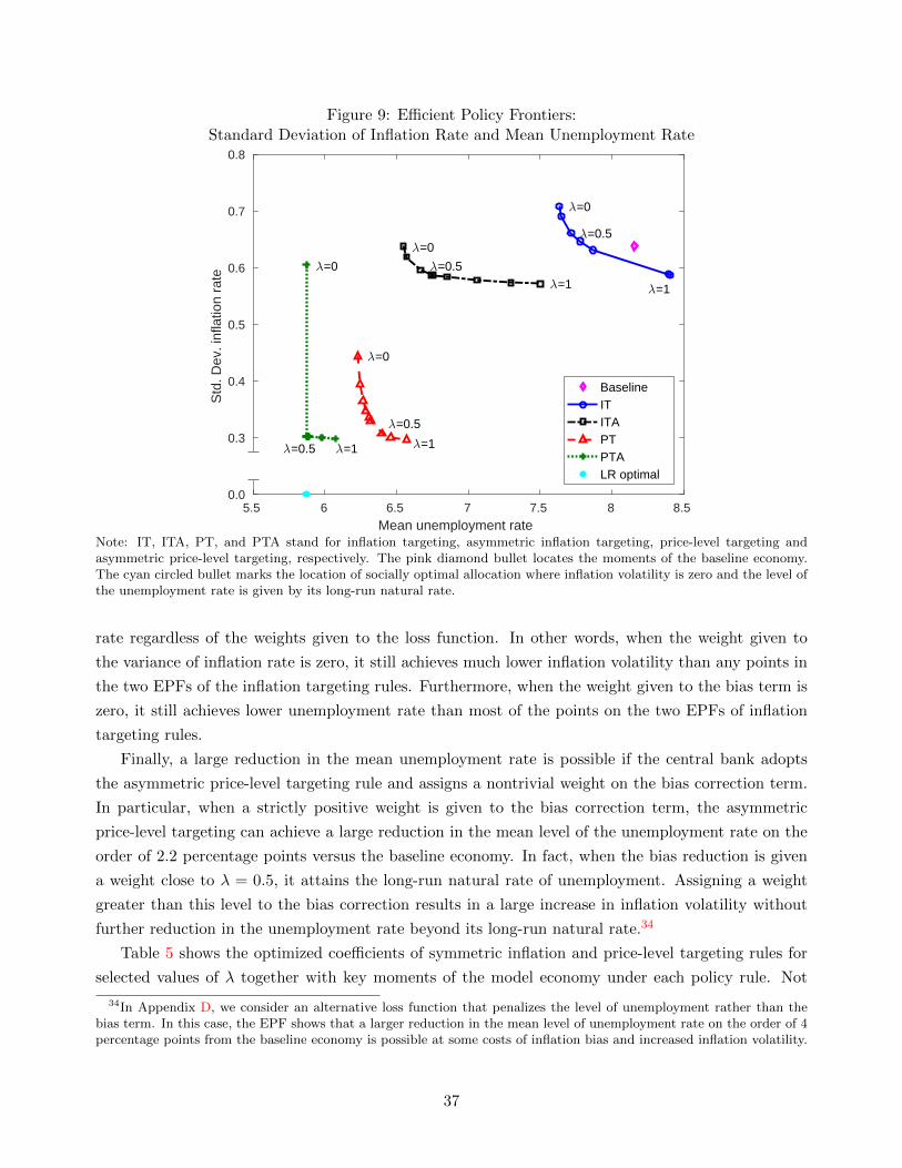
Figure 9: Efficient Policy Frontiers:Standard Deviation of Inflation Rate and Mean Unemployment Rate

5.5 6 6.5 7 7.5 8 8.5Mean unemployment rate

0.0

0.3

0.4

0.5

0.6

0.7

0.8

Std

. Dev

. inf

latio

n ra

te λ=0

λ=0.5

λ=1

λ=0

λ=0.5 λ=1

λ=0

λ=0.5

λ=1

λ=0

λ=0.5 λ=1

BaselineITITAPTPTALR optimal

Note: IT, ITA, PT, and PTA stand for inflation targeting, asymmetric inflation targeting, price-level targeting andasymmetric price-level targeting, respectively. The pink diamond bullet locates the moments of the baseline economy.The cyan circled bullet marks the location of socially optimal allocation where inflation volatility is zero and the level ofthe unemployment rate is given by its long-run natural rate.

rate regardless of the weights given to the loss function. In other words, when the weight given to

the variance of inflation rate is zero, it still achieves much lower inflation volatility than any points in

the two EPFs of the inflation targeting rules. Furthermore, when the weight given to the bias term is

zero, it still achieves lower unemployment rate than most of the points on the two EPFs of inflation

targeting rules.

Finally, a large reduction in the mean unemployment rate is possible if the central bank adopts

the asymmetric price-level targeting rule and assigns a nontrivial weight on the bias correction term.

In particular, when a strictly positive weight is given to the bias correction term, the asymmetric

price-level targeting can achieve a large reduction in the mean level of the unemployment rate on the

order of 2.2 percentage points versus the baseline economy. In fact, when the bias reduction is given

a weight close to λ = 0.5, it attains the long-run natural rate of unemployment. Assigning a weight

greater than this level to the bias correction results in a large increase in inflation volatility without

further reduction in the unemployment rate beyond its long-run natural rate.34

Table 5 shows the optimized coefficients of symmetric inflation and price-level targeting rules for

selected values of λ together with key moments of the model economy under each policy rule. Not

34In Appendix D, we consider an alternative loss function that penalizes the level of unemployment rather than thebias term. In this case, the EPF shows that a larger reduction in the mean level of unemployment rate on the order of 4percentage points from the baseline economy is possible at some costs of inflation bias and increased inflation volatility.

37

Table 5: Optimized Rules:Inflation Targeting vs. Price-Level Targeting

Inflation targeting Price-level targeting1. λ 0.00 0.50 1.00 0.00 0.50 1.002. ρπ 0.50 0.77 12.51 - - -3. ρΠ - - - 0.04 0.40 3.874. ρπ∗ - - - - - -5. E(u) 7.63 7.72 8.41 6.23 6.40 6.576. E(π) -0.18 -0.19 -0.25 0.00 0.00 0.007. S.D.(u) 5.91 5.44 5.09 4.28 2.95 2.818. S.D.(π) 0.71 0.66 0.59 0.44 0.31 0.309. Skewness(u) 1.02 1.54 3.44 0.76 1.95 2.1210. Skewness(π) -0.76 -1.14 -3.40 -0.61 -1.50 -1.5411. E(pδ) 1.32 1.33 1.34 1.33 1.33 1.3412. Frequency of ZLB., pct. 2.08 3.42 9.74 0.77 4.02 9.3513. Mean MP. shock, bps. 0.37 1.00 30.85 0.75 16.48 176.3914. Loss function value 3.10 3.88 3.46 0.13 0.61 0.8815. Welfare of workers, CE 0.01 0.01 -0.03 0.38 0.37 0.3816. Welfare of shareholders, CE -0.29 -0.24 0.47 -2.23 -2.24 -2.2317. Aggregate welfare, CE -0.01 -0.01 -0.01 0.25 0.24 0.25

Note: We impose 0.5 ≤ ρπ ≤ 20 and 0.01 ≤ ρΠ ≤ 4 in the optimization, while ρπ∗ and σπ∗ are set equal to zero. Mean MPshock is the annualized mean of monetary policy shocks (both contemporaneous and anticipated news shocks) requiredto satisfy the ZLB constraint. CE stands for consumption equivalent that needs to be given to the baseline economy toachieve the same level of welfare.

surprisingly, as the loss function assigns a greater weight on the stabilization of the inflation gap, the

reaction coefficient to the inflation gap and price-level gap are increased (lines 2 and 3).35 Consequently,

the frequency of a binding ZLB constraint and the sizes of anticipated monetary policy shocks are

substantially higher (lines 12 and 13), and the flip side is a larger bias in the mean unemployment rate

(line 5). The price-level targeting rule dominates inflation targeting in terms of bias reduction in the

unemployment rate regardless of the value of λ. Furthermore, the optimized price-level targeting rules

eliminate deflation bias in contrast to inflation targeting rules (line 6). Finally, higher order moments

shown in lines 7∼10 also confirm the improved stabilization properties of the price-level targeting

rule in terms of variance reduction of the unemployment rate and the inflation rate and in terms of

correcting skewed distributions of these key macroeconomic variables. Overall, smaller loss function

values (line 14) associated with price-level targeting summarize the better performance of this rule

against the inflation targeting rule in our model economy 36

Lines 15 and 16 in Table 5 report the consumption equivalents that need to be given to the agents

in the baseline economy to be indifferent between the economy under the optimized policy rules and

the baseline economy. As such, positive numbers represent welfare improvement and negative numbers

welfare deterioration with respect to the baseline economy.37 What is notable about the welfare results

35It is notable that so called Taylor principle is not applied in the case of inflation targeting. In fact, inflation targetingrule with λ = 0 hits the lower bound ρπ = 0.50.

36Loss function values cannot be compared across different values of λ as they represent different preferences. Howeverfor a given λ, loss function values can be compared for different policy rules.

37All welfare values are based on a first order approximation. The presence of multiple anticipated news shocks tosatisfy the ZLB constraint in expectations creates a large number of auxiliary variables to limit the lag structure of the

38

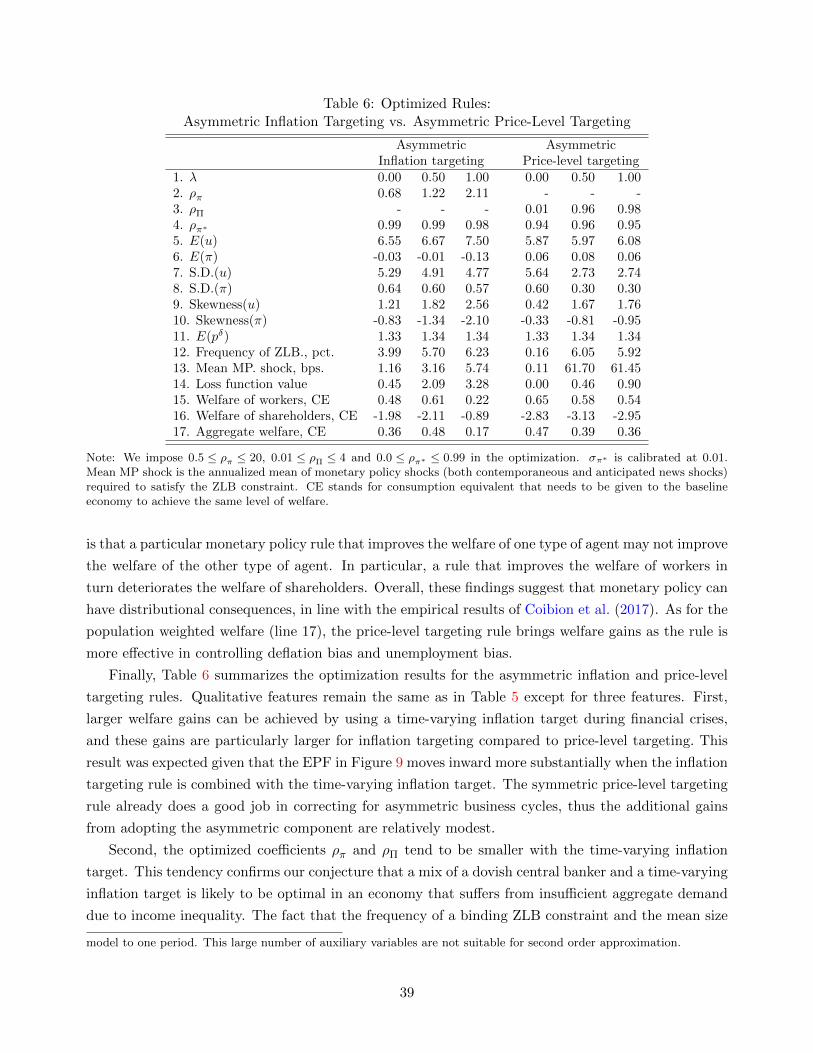
Table 6: Optimized Rules:Asymmetric Inflation Targeting vs. Asymmetric Price-Level Targeting

Asymmetric AsymmetricInflation targeting Price-level targeting

1. λ 0.00 0.50 1.00 0.00 0.50 1.002. ρπ 0.68 1.22 2.11 - - -3. ρΠ - - - 0.01 0.96 0.984. ρπ∗ 0.99 0.99 0.98 0.94 0.96 0.955. E(u) 6.55 6.67 7.50 5.87 5.97 6.086. E(π) -0.03 -0.01 -0.13 0.06 0.08 0.067. S.D.(u) 5.29 4.91 4.77 5.64 2.73 2.748. S.D.(π) 0.64 0.60 0.57 0.60 0.30 0.309. Skewness(u) 1.21 1.82 2.56 0.42 1.67 1.7610. Skewness(π) -0.83 -1.34 -2.10 -0.33 -0.81 -0.9511. E(pδ) 1.33 1.34 1.34 1.33 1.34 1.3412. Frequency of ZLB., pct. 3.99 5.70 6.23 0.16 6.05 5.9213. Mean MP. shock, bps. 1.16 3.16 5.74 0.11 61.70 61.4514. Loss function value 0.45 2.09 3.28 0.00 0.46 0.9015. Welfare of workers, CE 0.48 0.61 0.22 0.65 0.58 0.5416. Welfare of shareholders, CE -1.98 -2.11 -0.89 -2.83 -3.13 -2.9517. Aggregate welfare, CE 0.36 0.48 0.17 0.47 0.39 0.36

Note: We impose 0.5 ≤ ρπ ≤ 20, 0.01 ≤ ρΠ ≤ 4 and 0.0 ≤ ρπ∗ ≤ 0.99 in the optimization. σπ∗ is calibrated at 0.01.Mean MP shock is the annualized mean of monetary policy shocks (both contemporaneous and anticipated news shocks)required to satisfy the ZLB constraint. CE stands for consumption equivalent that needs to be given to the baselineeconomy to achieve the same level of welfare.

is that a particular monetary policy rule that improves the welfare of one type of agent may not improve

the welfare of the other type of agent. In particular, a rule that improves the welfare of workers in

turn deteriorates the welfare of shareholders. Overall, these findings suggest that monetary policy can

have distributional consequences, in line with the empirical results of Coibion et al. (2017). As for the

population weighted welfare (line 17), the price-level targeting rule brings welfare gains as the rule is

more effective in controlling deflation bias and unemployment bias.

Finally, Table 6 summarizes the optimization results for the asymmetric inflation and price-level

targeting rules. Qualitative features remain the same as in Table 5 except for three features. First,

larger welfare gains can be achieved by using a time-varying inflation target during financial crises,

and these gains are particularly larger for inflation targeting compared to price-level targeting. This

result was expected given that the EPF in Figure 9 moves inward more substantially when the inflation

targeting rule is combined with the time-varying inflation target. The symmetric price-level targeting

rule already does a good job in correcting for asymmetric business cycles, thus the additional gains

from adopting the asymmetric component are relatively modest.

Second, the optimized coefficients ρπ and ρΠ tend to be smaller with the time-varying inflation

target. This tendency confirms our conjecture that a mix of a dovish central banker and a time-varying

inflation target is likely to be optimal in an economy that suffers from insufficient aggregate demand

due to income inequality. The fact that the frequency of a binding ZLB constraint and the mean size

model to one period. This large number of auxiliary variables are not suitable for second order approximation.

39

of monetary policy shocks required to satisfy the ZLB constraint tend to be lower with the asymmetric

policy rules also suggests that such opportunistic adjustment of the inflation target can be an effective

tool in fighting the deflation bias imposed by the ZLB constraint.

Third, the population weighted welfare gains indicate that a conservative central banker tends to

reduce the size of overall welfare. In particular, the gains for workers generally decline as the weight

given to inflation stabilization is increased. Given that wage income is the major income source for

low income earners, a crucial factor for their welfare gains is how effective a particular monetary policy

rule is in reducing the bias in the unemployment rate.

8 Conclusion

The increase in income inequality in the United States during the recent decades has become a reason

for concern. This paper shows the important role that income inequality plays in the economy. By us-

ing a two-agent general equilibrium model, we show that income inequality can generate low aggregate

demand, deflation pressure, excessive credit growth and financial instability. The main mechanism to

deliver those results is the desire to accumulate financial wealth by shareholders motivated by their

“love of wealth” preferences. The paper shows that both occasional eruptions of endogenous finan-

cial crises and the zero lower bound constraint on the nominal interest rate generate distributions

of equilibrium prices and quantities that are highly skewed to the downside. In that environment,

a conservative central banker faces a trade-off between stabilizing inflation volatility and increasing

the mean level of the unemployment rate. This trade-off highlights the inefficiency of symmetric

monetary policy rules in the sense that a simultaneous reduction in inflation volatility and the mean

unemployment rate is feasible when an asymmetric policy rule is adopted.

Our results highlight the close link between income inequality and financial instability. While the

focus in this paper is on monetary policy issues, our findings suggest an important role for fiscal policy

as a macroprudential tool. In particular, redistribution policies that ameliorate income inequality

can potentially bring additional benefits in terms of preventing excessive credit growth, reducing the

probability of financial crises and further improving macroeconomic outcomes. We leave the study of

fiscal and macroprudential policies in our model economy for future research.

References

Adrian, Tobias and Fernando Duarte, “Financial Vulnerability and Monetary Policy,” StaffReports 804, Federal Reserve Bank of New York 2016.

, Nina Boyarchenko, and Domenico Giannone, “Vulnerable growth,” Staff Reports 794, Fed-eral Reserve Bank of New York 2016.

Atkinson, Anthony B., Thomas Piketty, and Emmanuel Saez, “Top Incomes in the Long Runof History,” Journal of Economic Literature, March 2011, 49 (1), 3–71.

40

Auclert, Adrien, “Monetary Policy and the Redistribution Channel,” Working Paper 23451, Na-tional Bureau of Economic Research May 2017.

and Matthew Rognlie, “Inequality and Aggregate Demand,” Technical Report 2016.

Aumann, Robert J., “Values of Markets with a Continuum of Traders,” Econometrica, 1975, 43(4), 611–646.

Bernanke, Ben S., “Monetary Policy for a New Era,” October 2017. paper prepared for ”RethinkingMacroeconomic Policy,” a conference held at the Peterson Institute for International Economics,Washington, October 12.

Blanchard, Olivier and Jordi Galı, “Real Wage Rigidities and the New Keynesian Model,” Journalof Money, Credit and Banking, 2007, 39, 35–65.

Blundell, Richard, Luigi Pistaferri, and Ian Preston, “Consumption Inequality and PartialInsurance,” American Economic Review, December 2008, 98 (5), 1887–1921.

Broda, Christian and Jonathan A. Parker, “The Economic Stimulus Payments of 2008 andthe aggregate demand for consumption,” Journal of Monetary Economics, 2014, 68, S20 – S36.Supplement issue: October 19-20, 2012 Research Conference on Financial Markets, Financial Policy,and Macroeconomic Activity Sponsored by the Study Center Gerzensee and the Swiss NationalBank.

Calvo, Guillermo A., “Staggered prices in a utility-maximizing framework,” Journal of MonetaryEconomics, 1983, 12 (3), 383 – 398.

Carroll, Christopher, Jiri Slacalek, Kiichi Tokuoka, and Matthew N. White, “The distri-bution of wealth and the marginal propensity to consume,” Quantitative Economics, 2017, 8 (3),977–1020.

Clarida, Richard, Jordi Galı, and Mark Gertler, “The Science of Monetary Policy: A NewKeynesian Perspective,” Journal of Economic Literature, December 1999, 37 (4), 1661–1707.

Coibion, Olivier, Yuriy Gorodnichenko, and Johannes Wieland, “The Optimal Inflation Ratein New Keynesian Models: Should Central Banks Raise Their Inflation Targets in Light of the ZeroLower Bound?,” Review of Economic Studies, 2012, 79 (4), 1371–1406.

, , Lorenz Kueng, and John Silvia, “Innocent Bystanders? Monetary policy and inequality,”Journal of Monetary Economics, 2017, 88 (C), 70–89.

Drautzburg, Thorsten, Jesus Fernandez-Villaverde, and Pablo Guerron-Quintana, “Po-litical Distribution Risk and Aggregate Fluctuations,” Working Paper 23647, National Bureau ofEconomic Research August 2017.

Drehmann, Mathias, Claudio Borio, and Kostas Tsatsaronis, “Anchoring CountercyclicalCapital Buffers: The role of Credit Aggregates,” International Journal of Central Banking, Decem-ber 2011, 7 (4), 189–240.

, , Leonardo Gambacorta, Gabriel Jimenez, and Carlos Trucharte, “Countercyclicalcapital buffers: exploring options,” BIS Working Papers 317, Bank for International Settlements2010.

41

Dupraz, Stephane, Emi Nakamura, and Jon Steinsson, “A Plucking Model of Business Cy-cles,” http://www.columbia.edu/~en2198/papers/plucking.pdf May 2017. Columbia UniversityWorking Paper.

Elsby, Michael, Bart Hobijn, and Aysegul Sahin, “The Decline of the U.S. Labor Share,”Brookings Papers on Economic Activity, 2013, 44 (2 (Fall)), 1–63.

Fisher, Jonas D.M., “On the Structural Interpretation of the Smets–Wouters Risk Premium Shock,”Journal of Money, Credit and Banking, 2015, 47 (2-3), 511–516.

Galı, Jordi, “Technology, Employment, and the Business Cycle: Do Technology Shocks ExplainAggregate Fluctuations?,” American Economic Review, March 1999, 89 (1), 249–271.

and Mark Gertler, “Inflation dynamics: A structural econometric analysis,” Journal of MonetaryEconomics, October 1999, 44 (2), 195–222.

, , and J. David Lopez-Salido, “European inflation dynamics,” European Economic Review,2001, 45 (7), 1237–1270.

Gertler, Mark, Luca Sala, and Antonella Trigari, “An Estimated Monetary DSGE Model withUnemployment and Staggered Nominal Wage Bargaining,” Journal of Money, Credit and Banking,2008, 40 (8), 1713–1764.

Gornemann, Nils, Keith Kuester, and Makoto Nakajima, “Doves for the Rich, Hawks for thePoor? Distributional Consequences of Monetary Policy,” International Finance Discussion Papers1167, Board of Governors of the Federal Reserve System (U.S.) May 2016.

Gourio, Francois, Anil K Kashyap, and Jae Sim, “The Tradeoffs in Leaning Against the Wind,”IMF Economic Review, March 2018, 66 (1), 70–115.

Guerrieri, Veronica and Guido Lorenzoni, “Credit Crises, Precautionary Savings, and the Liq-uidity Trap,” The Quarterly Journal of Economics, 2017, 132 (3), 1427–1467.

Hagedorn, Marcus and Iourii Manovskii, “The Cyclical Behavior of Equilibrium Unemploymentand Vacancies Revisited,” American Economic Review, September 2008, 98 (4), 1692–1706.

Hansen, Alvin H., “Economic Progress and Declining Population Growth,” The American EconomicReview, 1939, 29 (1), 1–15.

Havranek, Tomas, Marek Rusnak, and Anna Sokolova, “Habit formation in consumption: Ameta-analysis,” European Economic Review, 2017, 95, 142 – 167.

Hicks, John Richard, A contribution to the theory of the trade cycle, London: Clarendon Press,1972.

Jappelli, Tullio and Luigi Pistaferri, “Fiscal Policy and MPC Heterogeneity,” American EconomicJournal: Macroeconomics, October 2014, 6 (4), 107–36.

Jensen, Henrik, Ivan Petrella, Soren Hove Ravn, and Emiliano Santoro, “Leverage andDeepening Business Cycle Skewness,” CEPR Discussion Papers 12239, C.E.P.R. Discussion PapersAugust 2017.

Kalecki, Micha l, Selected Essays on the Dynamics of the Capitalist Economy 1933–1970, CambridgeUniversity Press, 1971.

42

Kaplan, Greg and Giovanni L. Violante, “A Model of the Consumption Response to FiscalStimulus Payments,” Econometrica, 2014, 82 (4), 1199–1239.

, Benjamin Moll, and Giovanni L. Violante, “Monetary Policy According to HANK,” Amer-ican Economic Review, March 2018, 108 (3), 697–743.

Karabarbounis, Loukas and Brent Neiman, “The Global Decline of the Labor Share*,” TheQuarterly Journal of Economics, 2013.

Keynes, John Maynard, The Economic Consequences of the Peace History of Economic ThoughtBooks, McMaster University Archive for the History of Economic Thought, 1919.

, The General Theory of Employment, Interest and Money, Macmillan, 1936. 14th edition, 1973.

, “The General Theory of Employment,” The Quarterly Journal of Economics, 1937, 51 (2), 209–223.

Kocherlakota, Narayana R., “Creating business cycles through credit constraints,” Quarterly Re-view, 2000, (Sum), 2–10.

Koh, Dongya, Raul Santaeulalia-Llopis, and Yu Zheng, “Labor Share Decline and Intellec-tual Property Products Capital,” Working Papers 927, Barcelona Graduate School of EconomicsSeptember 2016.

Krueger, Dirk, Kurt Mitman, and Fabrizio Perri, “Chapter 11 - Macroeconomics and HouseholdHeterogeneity,” in John B. Taylor and Harald Uhlig, eds., John B. Taylor and Harald Uhlig, eds.,Vol. 2 of Handbook of Macroeconomics, Elsevier, 2016, pp. 843 – 921.

Kumhof, Michael, Romain Ranciere, and Pablo Winant, “Inequality, Leverage, and Crises,”American Economic Review, 2015, 105 (3), 1217–45.

Linde, Jesper, Frank Smets, and Rafael Wouters, “Chapter 28 - Challenges for Central BanksMacro Models,” in John B. Taylor and Harald Uhlig, eds., John B. Taylor and Harald Uhlig, eds.,Vol. 2 of Handbook of Macroeconomics, Elsevier, 2016, pp. 2185 – 2262.

McKay, Alisdair and Ricardo Reis, “The Role of Automatic Stabilizers in the U.S. BusinessCycle,” Econometrica, 2016, 84 (1), 141–194.

, Emi Nakamura, and Jon Steinsson, “The Power of Forward Guidance Revisited,” AmericanEconomic Review, October 2016, 106 (10), 3133–3158.

Mitman, Kurt, Iourii Manovskii, and Marcus Hagedorn, “The Fiscal Multiplier,” 2017 Meet-ing Papers 1383, Society for Economic Dynamics 2017.

Nakata, Taisuke and Sebastian Schmidt, “Conservatism and liquidity traps,” Working PaperSeries 1816, European Central Bank June 2015.

Oscar Jorda, Moritz Schularick, and Alan Taylor, “Financial Crises, Credit Booms, and Ex-ternal Imbalances: 140 Years of Lessons,” IMF Economic Review, 2011, 59 (2), 340–378.

Parker, Jonathan A., Nicholas S. Souleles, David S. Johnson, and Robert McClelland,“Consumer Spending and the Economic Stimulus Payments of 2008,” American Economic Review,October 2013, 103 (6), 2530–53.

43

Paul, Pascal, “Historical Patterns of Inequality and Productivity around Financial Crises,” WorkingPaper Series 2017-23, Federal Reserve Bank of San Francisco 2017.

Piketty, Thomas and Emmanuel Saez, “Income Inequality in the United States, 19131998,” TheQuarterly Journal of Economics, 2003, 118 (1), 1–41.

Pissarides, Christopher A. and Barbara Petrongolo, “Looking into the Black Box: A Surveyof the Matching Function,” Journal of Economic Literature, June 2001, 39 (2), 390–431.

Rogoff, Kenneth, “The Optimal Degree of Commitment to an Intermediate Monetary Target,” TheQuarterly Journal of Economics, 1985, 100 (4), 1169–1189.

Sbordone, Argia M., “Prices and unit labor costs: a new test of price stickiness,” Journal ofMonetary Economics, March 2002, 49 (2), 265–292.

Schularick, Moritz and Alan M. Taylor, “Credit Booms Gone Bust: Monetary Policy, LeverageCycles, and Financial Crises, 1870-2008,” American Economic Review, April 2012, 102 (2), 1029–61.

Smets, Frank and Rafael Wouters, “Shocks and Frictions in US Business Cycles: A BayesianDSGE Approach,” American Economic Review, 2007, 97 (3), 586–606.

Solow, Robert, “The Future of Work: Why Wages Aren’t Keeping Up,” http://www.psmag.com/

business-economics/the-future-of-work-why-wages-arent-keeping-up August 2015. PacificStandard.

Summers, Lawrence H., “Demand Side Secular Stagnation,” American Economic Review, May2015, 105 (5), 60–65.

Taylor, John B., “Estimation and Control of a Macroeconomic Model with Rational Expectations,”Econometrica, September 1979, 47 (5), 1267–86.

, “A Historical Analysis of Monetary Policy Rules,” in “Monetary Policy Rules” NBER Chapters,National Bureau of Economic Research, Inc, April 1999, pp. 319–348.

Weber, Max, The Protestant Ethic and the Spirit of Capitalism, Routledge, Jul 2013.

Werning, Ivan, “Incomplete Markets and Aggregate Demand,” Technical Report 2016.

Woodford, Michael, “The Taylor Rule and Optimal Monetary Policy,” American Economic Review,May 2001, 91 (2), 232–237.

Yellen, Janet L., “Perspectives on Inequality and Opportunity from the Survey of ConsumerFinances,” https://www.federalreserve.gov/newsevents/speech/yellen20141017a.htm 2014.Speech by Janet L. Yellen, chair of the Board of Governors of the Federal Reserve System At theConference on Economic Opportunity and Inequality, Federal Reserve Bank of Boston, Boston,Massachusetts.

44

Online Appendix - Not Intended for Publication

A Non-Stochastic Steady State

A.1 Pinning Down the Endogenous Variables

To determine the steady state of the model, we guess the values of the borrowing level b and the defaultprobability pδ. We assume a zero inflation steady state, i.e., π = 1. Equation (49) then satisfies:

1 =[(1− ϕ)p1−γ

0 + ϕ]1/(1−γ)

, (A.1)

resulting in p0 = 1. Equations (46)∼(48) imply:

p0 =γµyπγ/(1− βϕ)

(γ − 1)yπ(γ−1)/(1− βϕ)= 1, (A.2)

which results in:

µ =γ − 1

γ. (A.3)

In the steady state qK = 1 from equation (50). Then, equation (23) determines:

r = 1/βK − (1− δ). (A.4)

Using this in equation (36), we define the steady state output-capital ratio as:

ρy/k ≡y

k=

1/βK − (1− δ)µα

. (A.5)

From the production function, we have:y

k= z

(nk

)1−α,

or equivalently

ρn/k ≡n

k=(ρy/k

z

)1/(1−α)

. (A.6)

Again from the production function, we derive output-labor ratio as:

ρy/n ≡y

n= z

(nk

)−α= zρ−αn/k. (A.7)

These ratios can be used to determine the levels of output and capital once the level of employment n isdetermined.

We determine the steady state job market tightness by calibrating the job finding rate from the data, i.e.,p(θ) = p. Using equation (A.7), we simplify the expression for the wage as:

w = ηµ(1− α)ρy/n + (1− η)bU + (1− ρ)η[βK − βW (1− p)]ξq. (A.8)

Equations (34) and (35) imply in steady state:

ξ

q= µ(1− α)ρy/n − w + (1− ρ)βK ξ

q. (A.9)

Equations (A.8) and (A.9) provide us with two equations for two unknowns, w and ξ/q. Substituting equation(A.8) in equation (A.9) and solving it for ξ/q yields:

J =ξ

q=

(1− η)[µ(1− α)ρy/n − bU

]1− (1− ρ)βK1− η[1− (1− p)βW/βK ]

. (A.10)

45

Using this in equation (43) yields the steady state wage.Since ξ/q = ξθ/p(θ) = ξθ/p, we have:

θ =p

ξ

(1− η)[µ(1− α)ρy/n − bU

]1− (1− ρ)βK1− η[1− (1− p)βW/βK ]

. (A.11)

This determines the matching function efficiency as:

ζ =p

θε. (A.12)

Note that we pin down ζ endogenously by matching the job finding rate of the model with the data. Thisrequires us to treat ζ as an endogenous variable, which always takes the same value as in the steady state.

From equation (32), we have the steady state employment stock as:

n =q

ρv =

q

ρθu. (A.13)

Substituting this expression in equation (27) yields:

u = 1− χ− (1− ρ)q

ρθu.

Solving this for u yields

u =1− χ

1 + (1− ρ)qθ/ρ.

The vacancy posting is determined as:v = θu,

and using this in equation (A.13) gives us the steady state employment stock. The levels of capital and outputare then given by:

y = ρy/nn, (A.14)

andk = ρ−1

n/kn. (A.15)

In a steady state where a default event does not occur:

cW = cN = (qB − 1) b+1

1− χ[wn+ (1− χ− n)bU ] , (A.16)

and

cK = b (1− qB)1− χχ− qK

δk

χ+rk

χ+

ΠY

χ+

ΠK

χ+T

χ, (A.17)

whereΠY = y − wn− rk − ξv, (A.18)

andΠK = qKx− x = 0. (A.19)

Substituting equations (A.18) and (A.19), the steady state version of the FOC for borrowing given by:

qB = βB(1− pδh), (A.20)

and the balanced budget constraint for government given by:

T = −(1− χ− n)bU + χbG(

1− 1

1 + i

)

46

into equation (A.17), we express the steady state consumption level of shareholders as:

cK(b) =1

χb[1− βW (1− pδh)](1− χ)− qKδk + y − wn− ξv − (1− χ− n)bU. (A.21)

Note that the right-hand side of the above has only one unknown, b. In order to pin down b, we equate theFOCs of the two agents regarding borrowing and lending, which results in

(βW − βK)(1− pδh) =ψ

[(1− s)cK(b)]−1/σc

[1 + b

(1− χχ

)]−1/σb

. (A.22)

Our initial guess b should satisfy equation (A.22) given our guess pδ. We now discuss how the guess solution pδ

can be validated.

A.2 Probability of Default

We envision a steady state in which there has been no default for a long time such that the lagged value ofpecuniary default cost has converged to zero, i.e., ν−1 = 0. In such an environment, if a default occurs today,the value of default cost becomes ν = γν . If a default does not occur today, the value of default cost becomesν = 0. If a default occurs again tomorrow after an episode of default today, ν′ = (1 + ρν)γν . If a default doesnot occur tomorrow after an incidence of default, ν′ = ρνγν . If a default occurs tomorrow after no incidence ofdefault today, ν′ = γν . If a default does not occur either today or tomorrow, ν′ = 0. Note that all of these fourcases are hypothetical in that a default does not occur in our steady state.

We denote four cases of consumption level tomorrow under the four scenarios by cDD, cDN , cND and cNN .These are given by:

cDD = [qB − (1− h)]b+1

1− χ[wn+ (1− χ− n)bU − (1 + ρν)γνy] , (A.23)

cDN = (qB − 1)b+1

1− χ[wn+ (1− χ− n)bU − ρνγνy] , (A.24)

cND = [qB − (1− h)]b+1

1− χ[wn+ (1− χ− n)bU − γνy] , (A.25)

and

cNN = (qB − 1)b+1

1− χ[wn+ (1− χ− n)bU ] . (A.26)

Note that all right-hand side variables are already determined above under the initial guess solution of pδ.However, this guess solution needs to be verified.

In the steady state, the continuation values of default and non-default are given by:

V D = βWpδ(

(cDD − scD)1−1/σc

1− 1/σc+ V D

)+ βW (1− pδ)

((cDN − scD)1−1/σc

1− 1/σc+ V N

)(A.27)

and

V N = βWpδ(

(cND − scN)1−1/σc

1− 1/σc+ V D

)+ βW (1− pδ)

((cNN − scN)1−1/σc

1− 1/σc+ V N

). (A.28)

By subtracting equation (A.27) from equation (A.28), one can derive ∆V (pδ) as:

∆V (pδ) = V D − V N

= βWpδ(

(cDD − scD)1−1/σc

1− 1/σc− (cND − scN)1−1/σc

1− 1/σc

)+βW (1− pδ)

((cDN − scD)1−1/σc

1− 1/σc− (cNN − scN)1−1/σc

1− 1/σc

).

47

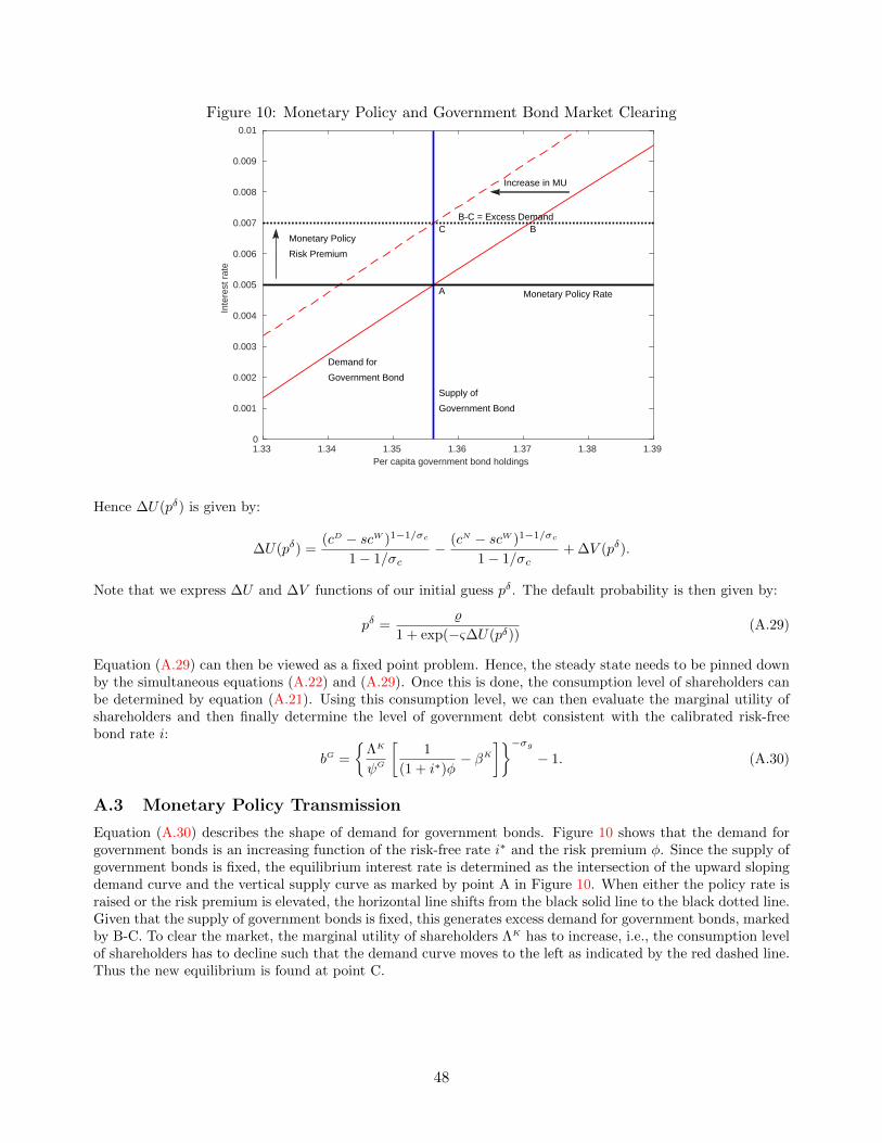
Figure 10: Monetary Policy and Government Bond Market Clearing

1.33 1.34 1.35 1.36 1.37 1.38 1.39Per capita government bond holdings

0

0.001

0.002

0.003

0.004

0.005

0.006

0.007

0.008

0.009

0.01

Inte

rest

rat

e

A

BC

Demand for

Government Bond

Supply of

Government Bond

Monetary Policy Rate

Monetary Policy

Risk Premium

Increase in MU

B-C = Excess Demand

Hence ∆U(pδ) is given by:

∆U(pδ) =(cD − scW )1−1/σc

1− 1/σc− (cN − scW )1−1/σc

1− 1/σc+ ∆V (pδ).

Note that we express ∆U and ∆V functions of our initial guess pδ. The default probability is then given by:

pδ =%

1 + exp(−ς∆U(pδ))(A.29)

Equation (A.29) can then be viewed as a fixed point problem. Hence, the steady state needs to be pinned downby the simultaneous equations (A.22) and (A.29). Once this is done, the consumption level of shareholders canbe determined by equation (A.21). Using this consumption level, we can then evaluate the marginal utility ofshareholders and then finally determine the level of government debt consistent with the calibrated risk-freebond rate i:

bG =

ΛK

ψG

[1

(1 + i∗)φ− βK

]−σg

− 1. (A.30)

A.3 Monetary Policy Transmission

Equation (A.30) describes the shape of demand for government bonds. Figure 10 shows that the demand forgovernment bonds is an increasing function of the risk-free rate i∗ and the risk premium φ. Since the supply ofgovernment bonds is fixed, the equilibrium interest rate is determined as the intersection of the upward slopingdemand curve and the vertical supply curve as marked by point A in Figure 10. When either the policy rate israised or the risk premium is elevated, the horizontal line shifts from the black solid line to the black dotted line.Given that the supply of government bonds is fixed, this generates excess demand for government bonds, markedby B-C. To clear the market, the marginal utility of shareholders ΛK has to increase, i.e., the consumption levelof shareholders has to decline such that the demand curve moves to the left as indicated by the red dashed line.Thus the new equilibrium is found at point C.

48

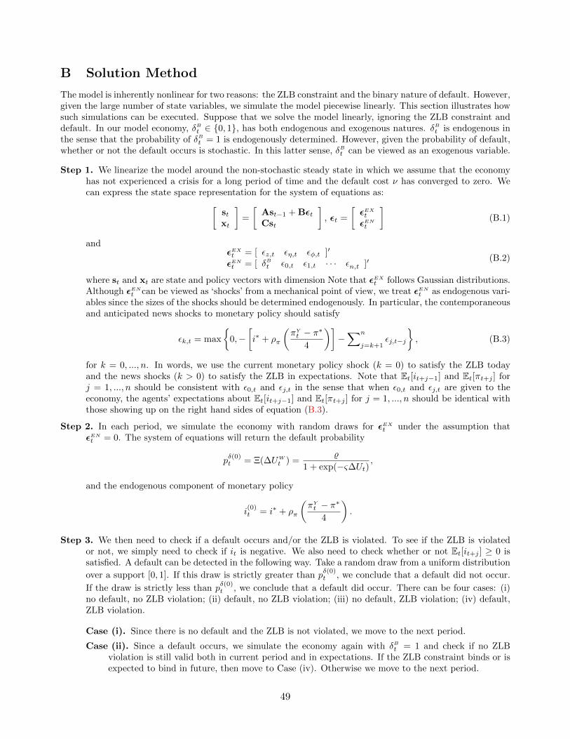
B Solution Method

The model is inherently nonlinear for two reasons: the ZLB constraint and the binary nature of default. However,given the large number of state variables, we simulate the model piecewise linearly. This section illustrates howsuch simulations can be executed. Suppose that we solve the model linearly, ignoring the ZLB constraint anddefault. In our model economy, δB

t ∈ 0, 1, has both endogenous and exogenous natures. δB

t is endogenous inthe sense that the probability of δB

t = 1 is endogenously determined. However, given the probability of default,whether or not the default occurs is stochastic. In this latter sense, δB

t can be viewed as an exogenous variable.

Step 1. We linearize the model around the non-stochastic steady state in which we assume that the economyhas not experienced a crisis for a long period of time and the default cost ν has converged to zero. Wecan express the state space representation for the system of equations as:[

stxt

]=

[Ast−1 + BεtCst

], εt =

[εEXt

εENt

](B.1)

andεEXt = [ εz,t εη,t εφ,t ]′

εENt = [ δB

t ε0,t ε1,t · · · εn,t ]′(B.2)

where st and xt are state and policy vectors with dimension Note that εEXt follows Gaussian distributions.

Although εENt can be viewed as ‘shocks’ from a mechanical point of view, we treat εEN

t as endogenous vari-ables since the sizes of the shocks should be determined endogenously. In particular, the contemporaneousand anticipated news shocks to monetary policy should satisfy

εk,t = max

0,−

[i∗ + ρπ

(πYt − π∗

4

)]−∑n

j=k+1εj,t−j

, (B.3)

for k = 0, ..., n. In words, we use the current monetary policy shock (k = 0) to satisfy the ZLB todayand the news shocks (k > 0) to satisfy the ZLB in expectations. Note that Et[it+j−1] and Et[πt+j ] forj = 1, ..., n should be consistent with ε0,t and εj,t in the sense that when ε0,t and εj,t are given to theeconomy, the agents’ expectations about Et[it+j−1] and Et[πt+j ] for j = 1, ..., n should be identical withthose showing up on the right hand sides of equation (B.3).

Step 2. In each period, we simulate the economy with random draws for εEXt under the assumption that

εENt = 0. The system of equations will return the default probability

pδ(0)t = Ξ(∆UW

t ) =%

1 + exp(−ς∆Ut),

and the endogenous component of monetary policy

i(0)t = i∗ + ρπ

(πYt − π∗

4

).

Step 3. We then need to check if a default occurs and/or the ZLB is violated. To see if the ZLB is violatedor not, we simply need to check if it is negative. We also need to check whether or not Et[it+j ] ≥ 0 issatisfied. A default can be detected in the following way. Take a random draw from a uniform distribution

over a support [0, 1]. If this draw is strictly greater than pδ(0)t , we conclude that a default did not occur.

If the draw is strictly less than pδ(0)t , we conclude that a default did occur. There can be four cases: (i)

no default, no ZLB violation; (ii) default, no ZLB violation; (iii) no default, ZLB violation; (iv) default,ZLB violation.

Case (i). Since there is no default and the ZLB is not violated, we move to the next period.

Case (ii). Since a default occurs, we simulate the economy again with δB

t = 1 and check if no ZLBviolation is still valid both in current period and in expectations. If the ZLB constraint binds or isexpected to bind in future, then move to Case (iv). Otherwise we move to the next period.

49

Case (iii). Since the ZLB constraint is violated (i(0)t < 0), where the superscript (0) indicates the number

of iterations in the ZLB loop, we set ε(1)0,t = −i(0)

t ε(1)j,t = max0,−Et[i(0)

t+j ] to satisfy Et[i(1)t+j ] ≥ 0.

We then simulate the economy again and check if the ZLB in current period or in expectationsis satisfied. This process cannot be done in one step because once the monetary policy shock ornews shock is given to the system, the economy reacts to the shocks, and the initial amounts ofmonetary policy shocks to satisfy the ZLB may not be enough. If the constraint is still not satisfied,

we set ε(2)0,t = −i(0)

t − i(1)t and ε

(2)j,t = −Et[i(0)

t+j ]−Et[i(1)t+j ], and simulate the economy again and check

if the ZLB is satisfied in current or in future expectations. If the ZLB is finally satisfied after Ssimulations, the final level of the monetary policy shock is given by:

ε(S)0,t = −

S∑s=0

i(s)t and ε

(S)j,t = −

S∑s=0

Et[i(s)t+j ] for j = 1, . . . N. (B.4)

An important thing in this iteration is to check whether or not a default occurs owing to theendogenous reaction of the economy to the monetary policy shock to satisfy the ZLB for a givensimulation number j. If a default occurs for this reason, then move to Case (iv). If not, move to thenext period.

Case (iv). In this case a crisis occurs and the ZLB binds. Hence we set δB

t = 1 and determine the sizeof the monetary policy shock according to equation (B.4). For a given simulation number j, weneed to check if a crisis occurs or not. In principle, it is logically possible, although not likely, thatthe economy gets itself out of the default mode due to the monetary policy shock. If this happens,move to Case (iii).

C System of Equations

There are variables 50 endogenous variables within the system:

Xt ≡

cKt bt lt ct πt qB

t it qKt kt rt

Tt ΛKt ΛW

t wt nt νt yt cWt mKt,t+1 ∆Ut

pδt vt ut θt p(θt) q(θt) zt mWt,t+1 Jt µt

wt Wt ηt p0,t PNt PD

t xt φt ΓWt ∆t

cDt cNt ΠYt ΠK

t cDDt cDN

t cNDt cNN

t Ωt ΓJt

The following provides the complete list of 50 equations for 50 endogenous variables:

lt = (1− hδB

t )bt−1

πt, (C.1)

ct = χcKt + (1− χ)cWt , (C.2)

Tt = (1− χ− nt)bU + χ

(bGt−1

πt− bGt

1 + it

), (C.3)

ΛK

t = (cKt − scKt−1)−1/σc , (C.4)

mK

t,t+1 = βKΛKt+1

ΛKt

, (C.5)

1 = Et[mK

t,t+1

(rt+1 + (1− δ)qK

t+1

qKt φt

)], (C.6)

1

1 + it= Et

[mK

t,t+1

φtπt+1

]+ψG

ΛKt

(1 + bGt )−1/σg , (C.7)

50

qB

t = Et[mK

t,t+1(1− hpδt+1)1

πt+1

]+ψB

ΛKt

[1 + bt

(1− χχ

)]−1/σb

, (C.8)

qB

t = Et[mW

t,t+1(1− hpδt+1)1

πt+1

], (C.9)

cWt = qB

t bt − lt +1

1− χ[wtnt + (1− χ− nt)bU − νtyt] , (C.10)

νt = ρννt−1 + γνδB

t , (C.11)

ΛW

t = (cWt − scWt−1)−1/σc , (C.12)

mW

t,t+1 = βWΛWt+1

ΛWt

, (C.13)

∆Ut =(cDt − scWt−1)1−1/σc

1− 1/σc−

(cNt − scWt−1)1−1/σc

1− 1/σc(C.14)

+βWEt

[pδt+1

((cDDt+1 − scDt )1−1/σc

1− 1/σc−

(cNDt+1 − scNt )1−1/σc

1− 1/σc

)]

+βWEt

[(1− pδt+1)

((cDNt+1 − scDt )1−1/σc

1− 1/σc−

(cNNt+1 − scNt )1−1/σc

1− 1/σc

)],

cDt = qB

t bt − (1− h)bt−1

πt+

1

1− χ[wtnt + (1− χ− nt)bU − (ρννt−1 + γν)yt] , (C.15)

cNt = qB

t bt −bt−1

πt+

1

1− χ[wtnt + (1− χ− nt)bU − ρννt−1yt] , (C.16)

cDD

t = qB

t bt − (1− h)bt−1

πt+

1

1− χ[wtnt + (1− χ− nt)bU − [ρν(ρννt−2 + γν) + γν ]yt] , (C.17)

cDN

t = qB

t bt −bt−1

πt+

1

1− χ[wtnt + (1− χ− nt)bU − ρν(ρννt−2 + γν)yt] , (C.18)

cND

t = qB

t bt − (1− h)bt−1

πt+

1

1− χ[wtnt + (1− χ− nt)bU − (ρνρννt−2 + γν)yt] , (C.19)

cNN

t = qB

t bt −bt−1

πt+

1

1− χ[wtnt + (1− χ− nt)bU − ρνρννt−2yt] , (C.20)

pδt =%

1 + exp(−ς∆Ut), (C.21)

ut = 1− χ− (1− ρ)nt−1, (C.22)

p(θt) = ζθεt, (C.23)

q(θt) = ζθε−1t , (C.24)

ξ

q(θt)= Jt, (C.25)

51

Jt = µt(1− α)ytnt− wt −

ϑ

2

(wtwt−1

− 1

)2

wt−1 + (1− ρ)Et[mK

t,t+1Jt+1], (C.26)

ΓWt = −1, (C.27)

ΓJt = −1− ϑ(

wtwt−1

− 1

)+ (1− ρ)Et

mK

t,t+1

ϑ

2

[(wt+1

wt

)2

− 1

], (C.28)

Ωt =ηt

ηt + (1− ηt)ΓJt /ΓWt, (C.29)

Wt =Ωt

1− ΩtJt, (C.30)

wt = bU + (1− ρ)Et[mW

t,t+1p(θt+1)Ωt+1

1− Ωt+1Jt+1

], (C.31)

wt = Ωtµt(1− α)ytnt

+ (1− Ωt)bU − Ωt

ϑ

2

(wtwt−1

− 1

)2

wt−1 (C.32)

+(1− ρ)Et[(

ΩtmK

t,t+1 − (1− Ωt)mW

t,t+1(1− p(θt+1)Ωt+1

1− Ωt+1

)ξ

q(θt+1)

],

PN

t = π(1−ε)γt

πεγt γµtyt + ϕEt

[mK

t,t+1PN

t+1

], (C.33)

PD

t = π(1−ε)(γ−1)t

πε(γ−1)t (γ − 1)yt + ϕEt

[mK

t,t+1PD

t+1

], (C.34)

p0,t =PNt

PDt

, (C.35)

πt =[(1− ϕ)p1−γ

0,t + ϕπε(1−γ)t−1

]1/(1−γ)

, (C.36)

qK

t = 1 + κ

(xtxt−1

− 1

)− Et

mK

t,t+1

κ

2

[(xt+1

xt

)2

− 1

], (C.37)

it = i∗ + ρπ

(πtπt−1πt−2πt−3 − π∗

4

)+

n∑j=0

εj,t−j , (C.38)

log zt = ρz log zt−1 + εz,t, (C.39)

log ηt = (1− ρη) log η + ρη log ηt−1 + εη,t, (C.40)

log φt = ρφ log φt−1 + εφ,t, (C.41)

yt = ∆−1t ztk

αt−1n

1−αt , (C.42)

∆t = πγt [(1− ϕ)p−γ0,t + ϕπ−vγt−1 ], (C.43)

nt = (1− ρ)nt−1 + q(θt)vt, (C.44)

52

kt = (1− δ)kt−1 + xt, (C.45)

rt = µtαytkt, (C.46)

θt =vtut, (C.47)

ΠY

t = yt − wtnt −ϑ

2

(wtwt−1

− 1

)2

wt−1nt − rtkt−1 − ξvt, (C.48)

ΠK

t = qK

t xt −

[xt +

κ

2

(xtxt−1

− 1

)2

xt−1

], (C.49)

cKt =bGt−1

πt− bGt

1 + it+ (lt − qB

t bt)1− χχ− 1

χqK

t [kt − (1− δ)kt−1] + rtkt−1 + ΠY

t + ΠK

t − Tt + νtyt . (C.50)

53

D Additional Results

D.1 Replication of Paul (2017)

In what sense can the moments shown in Table 3 can be considered representative of reality? To answer thisquestion, we replicate the empirical exercise of Paul (2017): we test the predictive power of credit in forecastingthe probability of financial crises, with and without controlling for income inequality using our simulated data.Specifically, we replicate Paul (2017)’s early warning signal model using the binary data of crisis indicator duringour stochastic simulation. The logit model is specified as:

log

(P [δB

t = 1|·]P [δB

t = 0|·]

)= αk + β1Zt−4 + β2Xt−4 + ut

where Zt−4 is the income inequality and Xt−4 is other control variables. The following table shows the estimationresults using our simulation data.

Table 7: Replicating the Logit Estimation Using Simulated Data

(1) (2) (3)

Creditt−4 1.342∗∗ - 1.007∗

(0.5927) - (0.597)[0.017] [0.013]

Shareholders Income Sharet−4 - 2.349∗∗∗ 2.111∗∗

- (0.774) (0.780)[0.030] [0.027]

Note: Parentheses are for standard errors and square brackets are formarginal effects.

As in Paul (2017), the credit variable predicts financial crises in our simulated economy as reported in column(1). However, column (2) shows that the share of shareholders predicts financial crises as well. Finally, column(3) reports that once we control for income inequality, the credit variable loses its predictive power. Theseare the stylized facts emphasized by Paul (2017) and our model can replicates them quite well. In particular,the marginal effects of credit and income inequality shown in squared brackets are quite comparable to thosereported in his study.

D.2 Monetary Policy Shocks to Satisfy the ZLB Constraint

Figure 11 shows the annualized unconditional and conditional means of monetary policy shocks (both contem-poraneous and anticipated news shocks) that are used to satisfy the ZLB constraint in our baseline economy.The former measures unconditional tightening effects due to the ZLB constraint. As such, the sum of uncon-ditional means represents a constant deflationary force facing the economy due to the ZLB constraint for anygiven period. The latter measures tightening effects conditioned upon any of 41 shocks being positive due toeither a presently binding ZLB constraint or the past expectations that the constraint would be binding in thenear term. As such, the sum of the conditional means represents a typical magnitude of tightening during abinding ZLB episode.

D.3 Monetary Accommodation During Financial Crises

Figure 12 replicates the experiment shown in Figure 3 when both financial crises and the ZLB constraint arepresent for ranges of inflation targeting rules between 1 and 20 (upper three panels) and price-level targetingrules between 0.1 and 4 (lower three panels) and shows the reactions of aggregate output, the inflation rate andthe path of the policy rate. The results shown in Figure 12 appear to suggest that for both inflation targetingand price-level targeting rules, the more hawkish the central banker is, the more monetary accommodation sheprovides to the economy during a financial crisis.

54

Figure 11: Means of Monetary Policy Shocks to Satisfy the ZLB Constraint(a) Unconditional mean

0 10 20 30 40

Periods

0

0.02

0.04

0.06

0.08

0.1

0.12

0.14

Perc

ent, a

nnual

(b) Conditional mean

0 10 20 30 40

Periods

0

0.2

0.4

0.6

0.8

1

1.2

1.4

Perc

ent, a

nnual

Notes: The figure shows the annualized unconditional and conditional means of monetary policy shocks used to satisfythe ZLB constraint in our baseline economy with financial crises and the ZLB constraint. The period marked as 0 on thehorizontal axis corresponds to contemporaneous shocks. The rest of the periods show the sizes of 40 anticipated newsshocks at each horizon.

Figure 12: Monetary Policy Accommodation During a Financial Crisis

0 20 40-10

-8

-6

-4

-2

0

2

Infla

tio

n t

arg

etin

g

(a) Output, pct

ρπ=1

ρπ=20

0 20 40-6

-4

-2

0

2(b) Inflation, ann. ppt

0 20 40-0.5

0

0.5

1

1.5

2

2.5

3(c) Nominal rate, ppt

0 20 40-10

-8

-6

-4

-2

0

2

Price

-le

ve

l ta

rge

tin

g

(d) Output, pct

ρΠ

=0.1

ρΠ

=4

0 20 40-6

-4

-2

0

2(e) Inflation, ann. ppt

0 20 40-0.5

0

0.5

1

1.5

2

2.5

3(f) Nominal rate, ppt

Notes: We use the same sequence of adverse risk-premium shocks as in Figure 3 when both financial crises and theZLB constraint are present for different values of the inflation reaction coefficient ρπ in the top panels and for differentreaction coefficient for price-level deviation ρΠ in the bottom panels.

55

D.4 Distributions of Key Endogenous Variables under Optimized Rules

Figures 13 and 14 show the exact shapes of the distributions for inflation and output in deviations from theirnon-stochastic steady state under the optimized symmetric and asymmetric rules, respectively.

Figure 13: Distributions of Inflation and Output underOptimized Inflation and Price-Level Targeting Rules with λ = 0.5

-3 -2 -1 0 1 20

0.5

1

1.5

2

2.5(a) Inflation rate (ppt)

-20 -10 0 100

0.05

0.1

0.15

0.2

0.25(b) Output (pct)

Baseline Inflation targeting Price-level targeting

Notes: The figure plots the distributions of inflation and output in deviations from their non-stochastic steady statedepending on the presence of financial crises and the ZLB constraint using kernel density estimates of simulated data.

Figure 14: Distributions of of Inflation and Output underOptimized Asymmetric Inflation and Price-Level Targeting Rules with λ = 0.5

-3 -2 -1 0 1 20

0.5

1

1.5

2

2.5(a) Inflation rate (ppt)

-20 -15 -10 -5 0 5 100

0.05

0.1

0.15

0.2

0.25(b) Output (pct)

Baseline Asymmetric inflation targeting Asymmetric price-level targeting

Notes: The figure plots the distributions of inflation and output in deviations from their non-stochastic steady statedepending on the presence of financial crises and the ZLB constraint using kernel density estimates of simulated data.

56

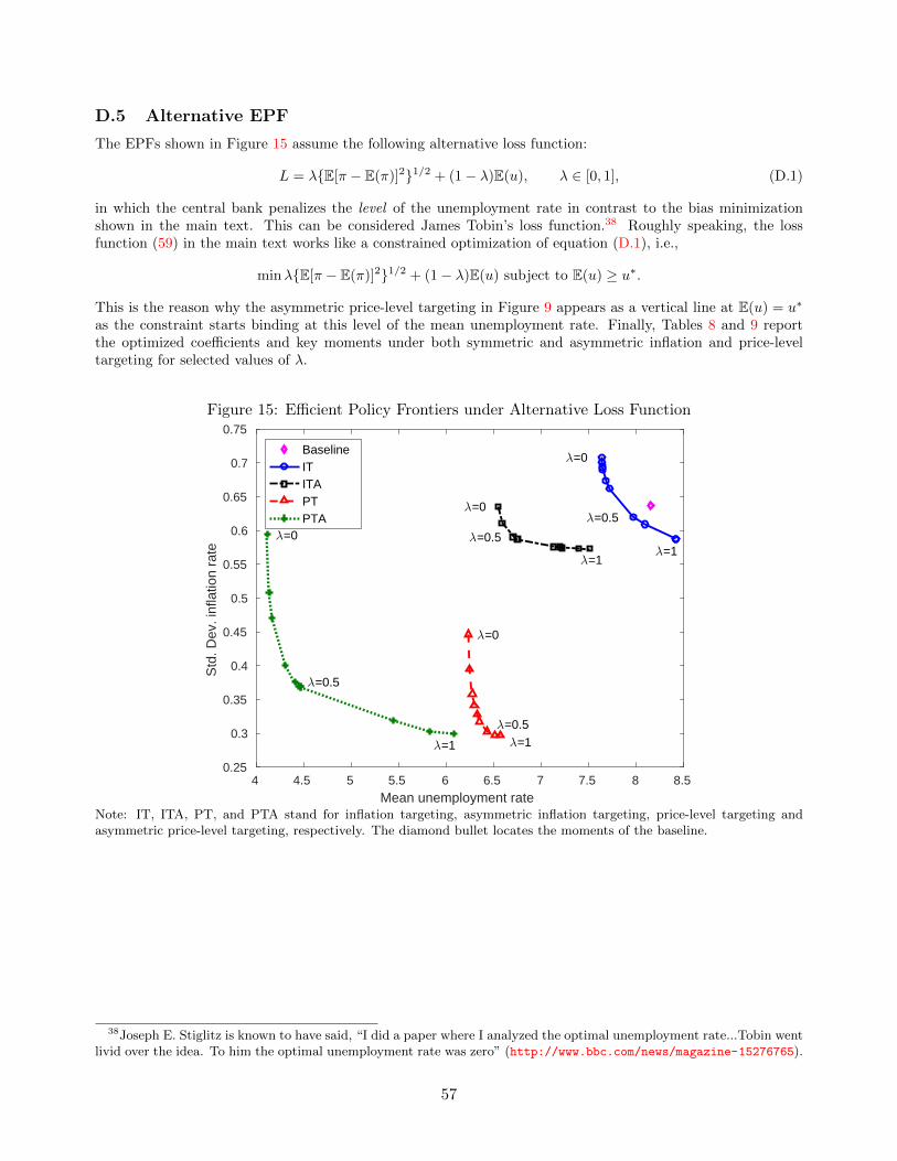
D.5 Alternative EPF

The EPFs shown in Figure 15 assume the following alternative loss function:

L = λE[π − E(π)]21/2 + (1− λ)E(u), λ ∈ [0, 1], (D.1)

in which the central bank penalizes the level of the unemployment rate in contrast to the bias minimizationshown in the main text. This can be considered James Tobin’s loss function.38 Roughly speaking, the lossfunction (59) in the main text works like a constrained optimization of equation (D.1), i.e.,

minλE[π − E(π)]21/2 + (1− λ)E(u) subject to E(u) ≥ u∗.

This is the reason why the asymmetric price-level targeting in Figure 9 appears as a vertical line at E(u) = u∗

as the constraint starts binding at this level of the mean unemployment rate. Finally, Tables 8 and 9 reportthe optimized coefficients and key moments under both symmetric and asymmetric inflation and price-leveltargeting for selected values of λ.

Figure 15: Efficient Policy Frontiers under Alternative Loss Function

4 4.5 5 5.5 6 6.5 7 7.5 8 8.5Mean unemployment rate

0.25

0.3

0.35

0.4

0.45

0.5

0.55

0.6

0.65

0.7

0.75

Std

. Dev

. inf

latio

n ra

te

λ=0

λ=0.5

λ=1

λ=0

λ=0.5

λ=1

λ=0

λ=0.5 λ=1

λ=0

λ=0.5

λ=1

BaselineITITAPTPTA

Note: IT, ITA, PT, and PTA stand for inflation targeting, asymmetric inflation targeting, price-level targeting andasymmetric price-level targeting, respectively. The diamond bullet locates the moments of the baseline.

38Joseph E. Stiglitz is known to have said, “I did a paper where I analyzed the optimal unemployment rate...Tobin wentlivid over the idea. To him the optimal unemployment rate was zero” (http://www.bbc.com/news/magazine-15276765).

57

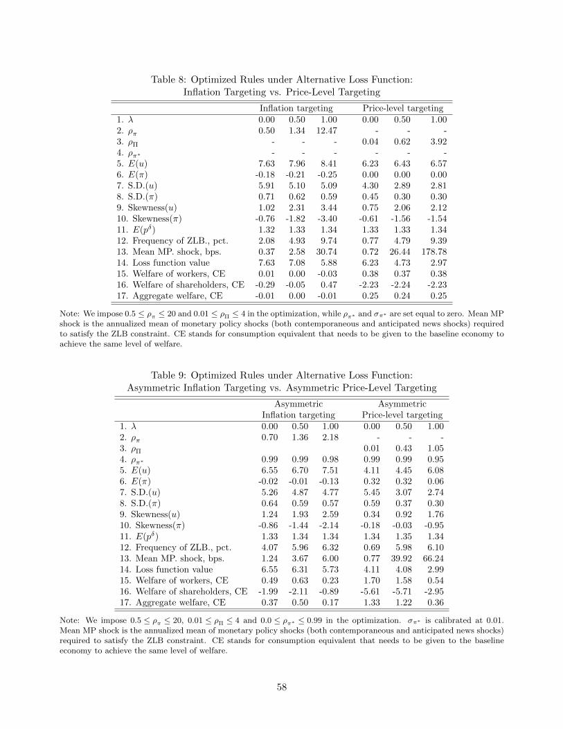
Table 8: Optimized Rules under Alternative Loss Function:Inflation Targeting vs. Price-Level Targeting

Inflation targeting Price-level targeting1. λ 0.00 0.50 1.00 0.00 0.50 1.002. ρπ 0.50 1.34 12.47 - - -3. ρΠ - - - 0.04 0.62 3.924. ρπ∗ - - - - - -5. E(u) 7.63 7.96 8.41 6.23 6.43 6.576. E(π) -0.18 -0.21 -0.25 0.00 0.00 0.007. S.D.(u) 5.91 5.10 5.09 4.30 2.89 2.818. S.D.(π) 0.71 0.62 0.59 0.45 0.30 0.309. Skewness(u) 1.02 2.31 3.44 0.75 2.06 2.1210. Skewness(π) -0.76 -1.82 -3.40 -0.61 -1.56 -1.5411. E(pδ) 1.32 1.33 1.34 1.33 1.33 1.3412. Frequency of ZLB., pct. 2.08 4.93 9.74 0.77 4.79 9.3913. Mean MP. shock, bps. 0.37 2.58 30.74 0.72 26.44 178.7814. Loss function value 7.63 7.08 5.88 6.23 4.73 2.9715. Welfare of workers, CE 0.01 0.00 -0.03 0.38 0.37 0.3816. Welfare of shareholders, CE -0.29 -0.05 0.47 -2.23 -2.24 -2.2317. Aggregate welfare, CE -0.01 0.00 -0.01 0.25 0.24 0.25

Note: We impose 0.5 ≤ ρπ ≤ 20 and 0.01 ≤ ρΠ ≤ 4 in the optimization, while ρπ∗ and σπ∗ are set equal to zero. Mean MPshock is the annualized mean of monetary policy shocks (both contemporaneous and anticipated news shocks) requiredto satisfy the ZLB constraint. CE stands for consumption equivalent that needs to be given to the baseline economy toachieve the same level of welfare.

Table 9: Optimized Rules under Alternative Loss Function:Asymmetric Inflation Targeting vs. Asymmetric Price-Level Targeting

Asymmetric AsymmetricInflation targeting Price-level targeting

1. λ 0.00 0.50 1.00 0.00 0.50 1.002. ρπ 0.70 1.36 2.18 - - -3. ρΠ 0.01 0.43 1.054. ρπ∗ 0.99 0.99 0.98 0.99 0.99 0.955. E(u) 6.55 6.70 7.51 4.11 4.45 6.086. E(π) -0.02 -0.01 -0.13 0.32 0.32 0.067. S.D.(u) 5.26 4.87 4.77 5.45 3.07 2.748. S.D.(π) 0.64 0.59 0.57 0.59 0.37 0.309. Skewness(u) 1.24 1.93 2.59 0.34 0.92 1.7610. Skewness(π) -0.86 -1.44 -2.14 -0.18 -0.03 -0.9511. E(pδ) 1.33 1.34 1.34 1.34 1.35 1.3412. Frequency of ZLB., pct. 4.07 5.96 6.32 0.69 5.98 6.1013. Mean MP. shock, bps. 1.24 3.67 6.00 0.77 39.92 66.2414. Loss function value 6.55 6.31 5.73 4.11 4.08 2.9915. Welfare of workers, CE 0.49 0.63 0.23 1.70 1.58 0.5416. Welfare of shareholders, CE -1.99 -2.11 -0.89 -5.61 -5.71 -2.9517. Aggregate welfare, CE 0.37 0.50 0.17 1.33 1.22 0.36

Note: We impose 0.5 ≤ ρπ ≤ 20, 0.01 ≤ ρΠ ≤ 4 and 0.0 ≤ ρπ∗ ≤ 0.99 in the optimization. σπ∗ is calibrated at 0.01.Mean MP shock is the annualized mean of monetary policy shocks (both contemporaneous and anticipated news shocks)required to satisfy the ZLB constraint. CE stands for consumption equivalent that needs to be given to the baselineeconomy to achieve the same level of welfare.

58