NBER WORKING PAPER SERIES

INCOME AND WEALTH VOLATILITY:EVIDENCE FROM ITALY AND THE U.S. IN THE PAST TWO DECADES

Conchita D'AmbrosioGiorgia Menta

Edward N. Wolff

Working Paper 26527http://www.nber.org/papers/w26527

NATIONAL BUREAU OF ECONOMIC RESEARCH1050 Massachusetts Avenue

Cambridge, MA 02138December 2019

D’Ambrosio and Menta gratefully acknowledge financial support from the Fonds National de la Recherche Luxembourg (Grants C18/SC/12677653 and 10949242). The views expressed herein are those of the authors and do not necessarily reflect the views of the National Bureau of Economic Research.

NBER working papers are circulated for discussion and comment purposes. They have not been peer-reviewed or been subject to the review by the NBER Board of Directors that accompanies official NBER publications.

© 2019 by Conchita D'Ambrosio, Giorgia Menta, and Edward N. Wolff. All rights reserved. Short sections of text, not to exceed two paragraphs, may be quoted without explicit permission provided that full credit, including © notice, is given to the source.

Income and Wealth Volatility: Evidence from Italy and the U.S. in the Past Two DecadesConchita D'Ambrosio, Giorgia Menta, and Edward N. WolffNBER Working Paper No. 26527December 2019JEL No. D31

ABSTRACT

Income volatility and wealth volatility are central objects of investigation for the literature on income and wealth inequality and dynamics. Here we analyse the two concepts in a comparative perspective for the same individuals in Italy and the U.S. over the last two decades. Contrary to our expectations, we find that in both countries wealth volatility reaches significantly higher values than income volatility, the effect being mostly driven by changes in the market value of real estate assets. We also show that there is more volatility in both dimensions in the United States and that the overall trend in both countries is increasing over time. We conclude by exploring volatility in consumption.

Conchita D'AmbrosioUniversity of Luxembourg 11, Porte des Sciences Esch-sur-Alzette 4366 Luxembourgconchita.dambrosio@uni.lu

Giorgia MentaUniversity of Luxembourg 11, Porte des Sciences Esch-sur-Alzette 4366 Luxembourggiorgia.menta@uni.lu

Edward N. WolffDepartment of EconomicsNew York University19 W. 4th Street, 6th FloorNew York, NY 10012and NBERedward.wolff@nyu.edu

1

1. Introduction

Income volatility has risen in a number of OECD countries in the recent past (Bartels and

Bönke, 2010, 2013; Daly and Valletta, 2008; Dynan et al., 2012; Jappelli and Pistaferri, 2010).

Most of the literature has focussed on the U.S., documenting a moderate to large increase in

household income volatility from the 1970s to the 2000s, with a variety of different data sources

and methods (DeBacker et al., 2012; Dynan et al., 2012; Hacker and Jacobs, 2008; Hacker,

2019; Shin and Solon, 2011; Winship, 2009). The financial lives of individuals and households

is increasingly subject to instability and unpredictability, due to changes in labour earnings,

access to welfare, and family composition. However, less is known about individual wealth

volatility in a comparative perspective, especially in relationship to income instability. Wealth

inequality is known to be typically higher than income inequality in the U.S. (Conley and

Glauber, 2008). These findings are confirmed by Fisher et al. (2016) and Johnson and Fisher

(2018), who look at the relationship between inequality and mobility in income, wealth, and

consumption for the same individuals. However, volatility is hardly ever addressed. One

exception is the work of Whalley and Yue (2009), who use Chinese data to investigate rural

income inequality and argue that higher income volatility exacerbates income inequality, as

well as poverty concerns.

In the light of higher income instability, how do individuals react to these unpredictable changes

in their financial streams? The Life-Cycle Theory suggests that wealth can act as form of self-

insurance against income shocks: in periods of diminished income, consumption smoothing is

ensured through the erosion of wealth and/or access to the credit market. The presence of

borrowing constraints might translate into even stronger incentives to accumulate wealth and

save ‘for a rainy day’. Following a life-cycle approach, one might then believe income volatility

in a given economy to be on average larger than wealth volatility: while the former is more

subject to life events and transitory conditions, the latter is run down in case of necessity in

order to converge towards a stable consumption path.

In this paper we investigate the relationship between income and wealth volatility in Italy and

in the United States, the only two countries for which, to the best of our knowledge, data is

2

available for more than a decade at the household and individual level. In order to do so, we

adopt a range of descriptive measures typically used in the realm of income and earnings

volatility, and apply them to both equivalised income and equivalised wealth. In particular, we

apply a battery of variance decomposition methods developed by Gottschalk and Moffit (1994,

2002, 2012), in order to disentangle a transitory component from a permanent component of

the variances of income and wealth. We base our empirical analysis by calculating individual

equivalised income and wealth from household longitudinal data from the United States (the

Panel Study of Income Dynamics, from here onwards PSID) and Italy (Banca d'Italia's Survey

on Household Income and Wealth, from here onwards SHIW). The panel dimension of these

datasets, together with their focus on income processes and assets distribution, make them the

perfect candidates for our purpose.

Several papers have documented an increase in household income volatility using PSID over

the last few decades. While most studies unanimously report an increasing trend in income

volatility in the U.S., there is no consensus on the magnitude of the effect – the differences

between estimates being mostly driven by measurement issues and sample selection. Using the

transitory component of the variance of log income, Hacker and Jacobs (2008) find that

household income volatility doubled between the late 1960s and the early 2000s; Winship

(2009), on the other hand, reports a more modest 30% increase in income volatility, measured

as the standard deviation of the two-year percentage change of income, around the same period.

See Dynan et al. (2012) for a thorough review of studies on earnings and household income

volatility in the U.S.. While wealth in PSID has been linked to macroeconomic volatility (Fang

et al., 2015; Heathcote and Perri, 2018; Stiglitz, 2012), little to nothing has been said on

household wealth volatility over time. One exception is Conley and Glauber (2008), who

measure wealth volatility in PSID as changes in average and median wealth across time and

find that more than one-third of adults experience at least one $1,000 drop in their inflation-

adjusted wealth before retirement.

With regard to Italy, Boeri and Brandolini in 2004 use SHIW to investigate whether the

impoverishment of Italian households was partly attributable to higher income volatility. They

3

perform their analysis at the individual level, using equivalised household income. Although

referring to income volatility, the authors focus their attention on income mobility measures

and report that mobility in Italy increased noticeably from the mid-1990s to the early 2000s.

Diaz-Serrano (2005), using the SHIW rotatory panel from 1986 to 2000, estimates transitory

shocks in labour income as the residuals from a Mincerian equation and finds a level of labour

income uncertainty (measured as the variance of individual level residuals over time) of 0.264

across the whole sample of male earners. Using more recent waves of the panel component of

the SHIW, Jappelli and Pistaferri (2010) highlight that in 2006 the variance of earnings per

adult equivalent is almost 0.5, higher than the variance of raw earnings. As for the analysis of

wealth, Brandolini et al. (2006) find a steady increase in wealth inequality in SHIW during the

1990s, mostly due to a larger concentration of financial wealth.

We analyse individual income and wealth volatility in PSID and SHIW across the years 2002

to 2014. Contrary to our initial expectations based on the life-cycle hypothesis, we find that in

both countries wealth volatility takes significantly higher values than income volatility. We

then investigate the determinants of wealth volatility by exploring the dynamics of assets prices

in Italy and the U.S., using data on rates of return to various components of wealth from the

Jordà-Schularick-Taylor Macrohistory Database. In particular, we decompose the variance of

wealth in order to disentangle the share of volatility that is due to changes in asset prices from

a residual component, and find that changes in the market values of stocks and real estate assets

drive most of the wealth volatility in our data. We also show that income and wealth volatility

are higher in the United States and that the overall trend in both countries is increasing over

time. Furthermore, we find evidence that the volatility of both income and wealth is higher

during the years of the Great Recession, more so for the U.S. than for Italy. We conclude by

exploring volatility in consumption and find that it predictably behaves in line with income

volatility in both countries.

Our paper contributes to the literature in several ways. We are the first, to the best of our

knowledge, to describe the evolution of income and wealth volatility for the same individuals

over time. We do so adopting a comparative approach for two countries and a unified

4

framework for each of the monetary variables. We further explore the channels that are likely

to drive our findings and, finally, we exploit sources of heterogeneity across households in order

to identify which groups are more vulnerable to income and wealth instability.

The remainder of the paper is organised as follows: Section 2 provides a review of the measures

of volatility that will be used in the paper, while Section 3 describes the data. Section 4 presents

results on income, wealth and consumption, and explores the role of rates of return in explaining

wealth volatility. Heterogeneity analysis is conducted in Section 5. Finally, Section 6 concludes.

2. Measuring volatility

A large strand of the literature has developed sophisticated econometric methods to estimate

variance components models. However, as argued by Shin and Solon (2011), these methods

rely on many assumptions and results are very sensitive to parametric specifications. This is

one of the reasons behind the popularity of a simpler class of descriptive measures, developed

by Gottschalk and Moffitt across the last few decades (see below for the references). Relying

on the literature on permanent income and permanent wealth, we can think of the logarithm of

each of our monetary variables (say log of income, 𝑦𝑦𝑖𝑖𝑖𝑖) as the following:

𝑦𝑦𝑖𝑖𝑖𝑖 = 𝑝𝑝𝑖𝑖 + 𝜀𝜀𝑖𝑖𝑖𝑖

where 𝑝𝑝𝑖𝑖 is a fixed permanent component with variance 𝜎𝜎𝑝𝑝2 (with mean zero and common across

all individuals) and 𝜀𝜀𝑖𝑖𝑖𝑖 is a transitory component analogous to an idiosyncratic shock with

variance 𝜎𝜎𝜀𝜀𝑖𝑖2 . The total variance of the observed monetary variable can be decomposed into:

𝜎𝜎𝑖𝑖2 = 𝜎𝜎𝑝𝑝2 + 𝜎𝜎𝜀𝜀𝑖𝑖2 .

Based on this underlying model, we decompose the variance of income and wealth into a

transitory and a permanent component. We here use two of the descriptive methods proposed

in the literature: the first, which we call MG1, is based on Moffitt and Gottschalk (2002, 2012);

the second, from here onwards MG2, was introduced by Gottschalk and Moffit (1994) and

subsequently applied in Gottschalk and Moffit (2009) and Moffit and Gottschalk (2012), among

5

others. See Chapter 6 in Jenkins (2011) for a thorough review of the econometric and

descriptive methods for the estimation of the transitory variance.

The first method, MG1, offers a straightforward way of decomposing the variance. Given a

long enough time interval s (based on data availability), it is possible to estimate the permanent

component of the variance as the covariance between income (wealth) at time t and income

(wealth) at time t-s. Subtracting the permanent variance to the observed variance yields an

estimate of the transitory component of the variance.

On the other hand, MG2 uses a window averaging method: instead of considering a time period

with respect to a number of lags, it requires the creation of a symmetric time window around a

given year. Then individual averages are computed across that interval, which gives an estimate

of the individual permanent income (wealth). The permanent variance is computed on the basis

of deviations of the permanent income (wealth) from the sample average, while the transitory

variance can be estimated as the average of individual variances of the difference between

observed income (wealth) and permanent income (wealth).

We then take what Moffitt and Zhang (2018) refer to as a measure of ‘gross volatility’, i.e. the

standard deviation of the individual differences in log income between one period and the next.

Although using a measure of dispersion of income changes such as the standard deviation or

the variance does not allow one to distinguish between a transitory and a permanent component,

Shin and Solon (2011) argue that the standard deviation is less sensitive to calendar changes

over time and that, under certain assumptions, it can provide less biased estimates of the

transitory variance than MG1. Hence we conduct sensitivity analysis using the standard

deviation of the two-year percentage changes in equivalent income and wealth as a measure of

volatility. This measure is systematically used in the literature to analyse the dynamics and

volatility individual earnings over time (see Dynan et al., 2012 for a review of the relevant

literature and methodology).

6

3. Data description

For our empirical application, we use individual panel data from the U.S. and Italy. For the first

country we rely on the Panel Study of Income Dynamics (PSID), while for Italy we use data

from the Banca d’Italia’s Survey on Household Income and Wealth (SHIW).

The latter began in 1965, with microdata available from 1977 onwards. It currently covers a

nationally representative sample of 8,000 Italian families (about 20,000 people), with a variety

of information on economic and financial behaviour of individuals, both at the individual and

family level. The SHIW was a repeated cross-section until 1989, when a randomly selected sub-

sample of about 4,000 previously interviewed families was selected to be part of the panel

component of the study. From 1989 onwards data were collected biannually (with the exception

of a three-year gap between 1995 and 1998), with the latest available wave dating 2016. The

year associated with the wave in SHIW is not the year when the interview took place, but the

year to which all variables refer to. For example, the 2016 wave refers to income and wealth of

year 2016, but was collected between 2017 and 2018.

The PSID is a longitudinal study collecting measures of income and other socio-economic

information for individuals living in the U.S.. It is currently the longest running panel study in

the world: starting with a nationally representative sample of 18,000 individuals surveyed in

1968, the 2017-released 40th wave of the study covers around 26,000 people, of which 3,500

from the original sample. While income in PSID is collected at the individual level, a wealth

supplement is only available at the family level, for years 1984, 1989, 1994, and biannually

from 1999 to 2017. For this reason we restrict the analysis to years 1999 to 2017. This choice

is also consistent with the SHIW, as data are available biannually from 1998 to 2016 (after a 3-

years discontinuity from 1995 to 1998). Since income - in PSID refers to the calendar year

before the year in which the interview took place, the time period we consider goes from 1998

to 2016, with biannual observations for both countries. Note that measures of wealth in PSID

refer instead to the calendar year of the interview.

7

In order to have a consistent time window and interview spells in the two countries, we focus

on biannual observations from 1998 to 2016, with the caveat that wealth observations in the

U.S. refer to the calendar year after.

Unlike in SHIW, measures of income in PSID are not net of taxes and transfers. Since 1992,

PSID stopped providing estimates on federal income tax payments, making it impossible to

directly derive a measure of net income from the available data for more recent years. However,

the National Bureau of Economic Research made available the Internet TAXSIM program, a

simulation tool aimed at calculating tax liabilities in the U.S. by assigning individuals to tax

units and tax filing statuses (see Feenberg and Coutts, 1993, for a thorough description of the

TAXSIM module). In particular, we rely on the method developed by Kimberlin, Kim and

Shaefer (2014) to compute federal and state income taxes between year 1999 and 2011 and

extend their procedure so to include subsequent years in our sample.1

Most of the literature looking at earnings or income volatility using PSID focuses only on

earnings of the male household head. As we are interested in individual welfare, we prefer to

keep the individual as our main unit of analysis without restricting our study to male earners

only. However, both in PSID and SHIW, wealth is only available at the household level. To

reconcile an individual-based analysis with the data restrictions, we decided to attribute

equivalised measures of income and wealth to individuals older than 15. Although we consider

a variety of equivalence scale parameters, we here present our analysis using the square-root

equivalence scale. Appendix A discusses how the choice of the scale parameter affects the

volatility measures we use throughout the paper.

As standard in the literature, we convert euros to dollars using PPP from the OECD data portal

and deflate all monetary measures with 2010 constant prices. We perform our analysis using a

logarithmic transformation of equivalised income and an inverse hyperbolic sine transformation

of equivalised wealth. The latter allows us to work with negative values without dropping them

from the dataset, as would happen with a logarithmic transformation. We are therefore able to

1 The process is straightforward, since Federal laws from 1960 to 2023 and State laws from 1977 to 2016 are already coded within the program.

8

take an unrestricted sample for wealth, while for income we drop negative values and attribute

the value 1 to zeros.2 We further trim the top 1% and the bottom 1% of the observations in our

samples (separately for each year in each of the two countries).

For MG1 we use 6-years lags to compute the permanent and transitory variance of income and

wealth, whereas for MG2 we use time window averaging 5 years.3

Because of the longitudinal nature of the measures described above, we further restrict the

sample to individuals who are observed in at least two waves before and one wave after the

current interview. The final estimation sample spans from year 2002 to 2012, retrospectively

and prospectively using information collected in years 1998, 2000, and 2014. It covers 11,458

individuals from Italy and 20,975 Americans, with non-missing information on income and

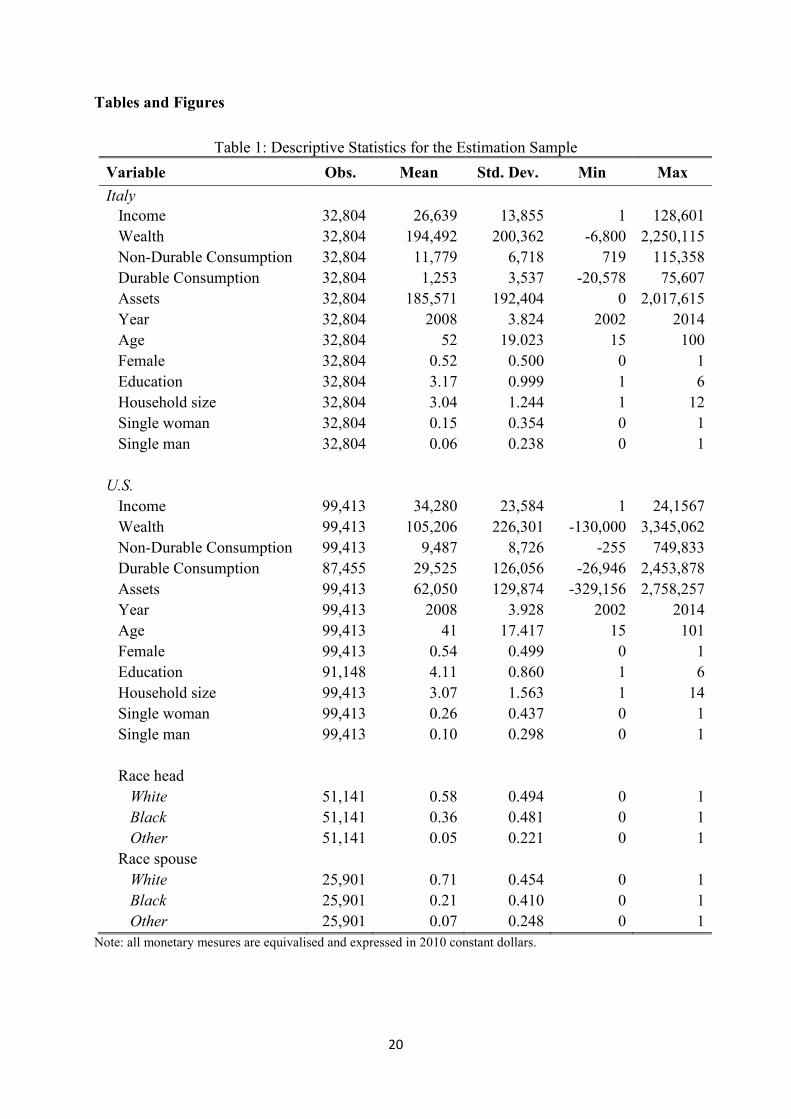
wealth for at least three consecutive periods. Table 1 summarises the general characteristics of

the estimation sample for the two countries.

4. Results

4.1 Income and Wealth

We here look at the evolution of the trends in the permanent and transitory component of the

variance of income and wealth, as well as the standard deviation of individual changes from

one period to the next.

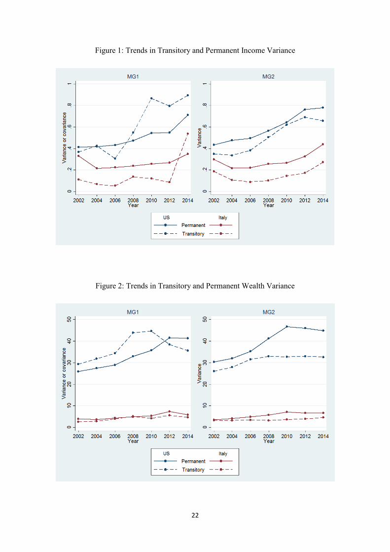
Figure 1 shows the evolution of the two descriptive Moffitt and Gottschalk variance

decomposition methods (MG1 and MG2) for incomes in the U.S. and in Italy. For each of the

methods used, the variance of income is decomposed into a transitory and into a permanent

component, the sum of which gives the total variance. The two methods seem to describe

similarly the evolution of the permanent component of income in both countries, while the same

cannot be said for the transitory component. The latter appears to be less smooth when using

2 In our estimation sample, after trimming, we only have 8 individuals in the U.S. with negative income and 0 in Italy. As for the zeroes, to which we attribute value 1, we have 414 cases in the U.S. (less than 0.5% of the American estimation sample) and 0 again for Italy. 3 We also use a 9-year centered window as a robustness check and find that results are qualitatively similar to the ones derived from the 5-year window MG2.

9

MG1 – the more so for the U.S.. Regardless of the method used, Figure 1 shows that income

volatility has been increasing since 2006, mostly due to increases in its transitory component,

more steeply for the U.S. than for Italy. In the latter country, in fact, income volatility appears

to be at most half of the U.S. levels.

To our knowledge, there are no other papers applying MG1 and MG2 to income data after the

mid-2000s to which we can compare our results. Moffitt and Gottschalk (2012) use MG1 and

MG2 to decompose the earnings variance of males aged 30 to 39, with PSID data, but their

series ends in 2004, the period after ours begins. Their estimates of the transitory variance for

the latest years in their sample have a magnitude of around 0.2, about half of the effect we find

at the beginning of our series. The trend in the transitory component of MG1 also seems to

mirror that in income inequality for the U.S., with a big jump over the Great Recession from

2006 to 2009, an abatement from 2009 to 2012, and then a strong upward trend from 2012 to

2015 (see Wolff, 2017, for income inequality trends based on the Survey of Consumer

Finances). The permanent component of MG1 shows a similar pattern over time, though with

smaller slopes (more attenuated changes). Both the permanent and transitory components of

MG2 show a more or less continuous increase over time. When it comes to the Italian case, the

trends in both MG1 and MG2 follow more of a U-shaped pattern, slowly increasing around the

Great Recession. With regard to the magnitude of income volatility in Italy, in the early 2000s,

we find our transitory income variance estimates to be in line with the estimates size of Diaz-

Serrano (2005). The overall variance of log income, i.e. the sum of the permanent and transitory

component of the MG1 variance, appears to be slightly lower than the figure of 0.45 found by

Jappelli and Pistaferri (2010) using SHIW between 1995 and 2005. However, with respect to

these authors, our sample is selected differently (e.g. we do not exclude retirees, whose stable

pension income might partly explain our lower figures), and we use net equivalised income

instead of earnings.

Figure 2 mirrors Figure 1, describing the evolution of wealth volatility in Italy and the U.S.. In

both countries we can see that wealth volatility seems to have increased more steeply in

concurrence of the Great Recession, more so in the U.S. than in Italy. Although, to the best of

10

our knowledge, no other paper applies MG1 and MG2 to wealth, we can still draw a parallel

between the evolution of the variance of wealth and wealth inequality in the U.S. and in Italy.

Wealth inequality in the U.S. was flat from 2004 to 2007, spiked upward from 2007 to 2010,

and then rose modestly after that (see Wolff, 2017). Here the transitory component of MG1

tracks well with this pattern from 2006 to 2012 but then shows a decline from 2012 to 2014. In

contrast, the permanent component of MG1 as well as both the permanent and transitory

components of MG2 shows a more or less continuous rise over the whole period. As for Italy,

Dagnes et al. (2018) find a modest decline in wealth inequality between 2000 and 2004,

followed by a steep upward trend peaking in 2012 and a sharp decline in 2014. These

movements appear to be mirrored by both the permanent and transitory MG1 components of

the variance of wealth in Italy, while the MG2 components show a flatter trend.

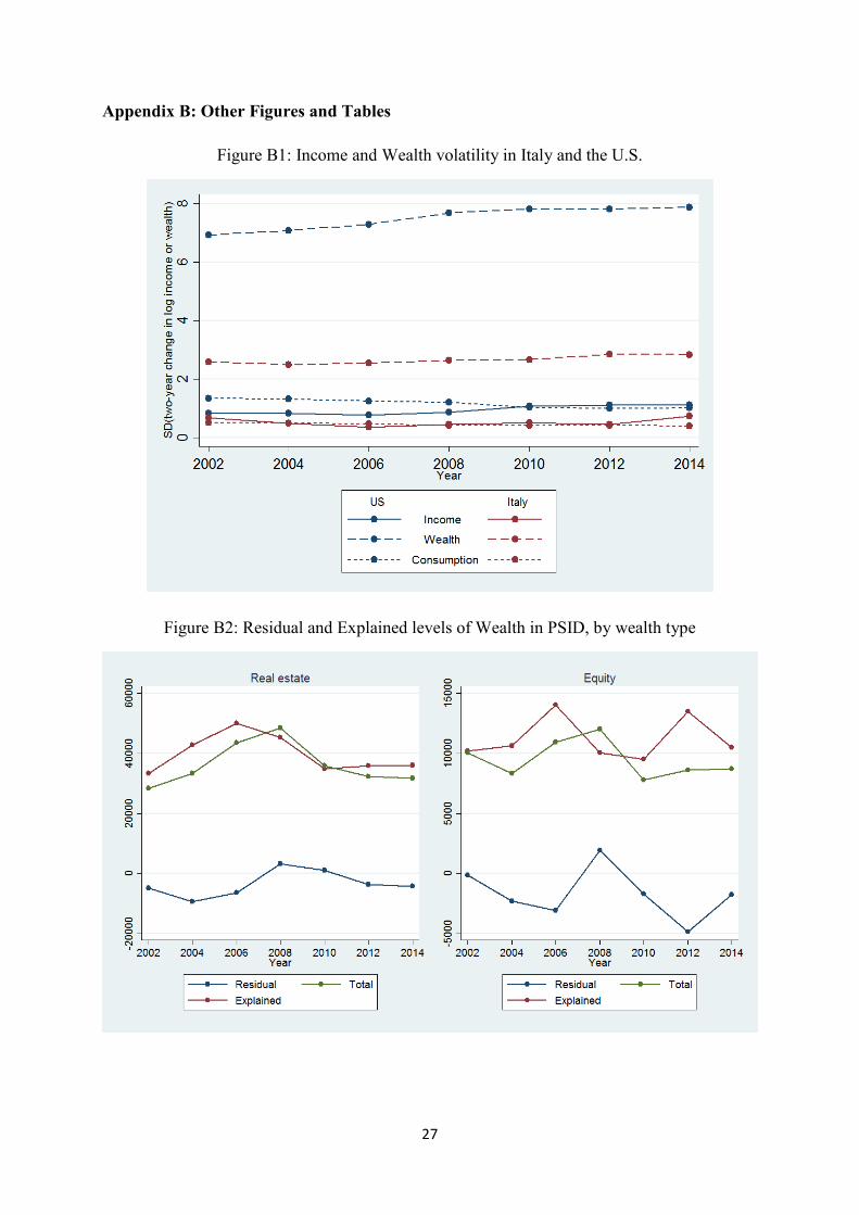
Two remarks can be made when comparing Figure 1 and Figure 2. First, wealth volatility

appears to be strikingly higher than income volatility, irrespectively of the time period or the

country considered. This is true not only for Moffitt and Gottschalk’s descriptive measures, but

also for the standard deviation of the two-year percent change in income and wealth (see Figure

B1 in the Appendix). The second remark is a methodological one: consistent with Jenkins

(2011), it appears that MG1 systematically overestimates the magnitude of the transitory

component of the variances of both income and wealth with respect to MG2, whereas the

contribution of the permanent component of the variances is robustly estimated across the two

methods.

So far, our results suggest that wealth is more volatile than income, at least in the countries and

years considered and the trend is increasing over time; in addition, both income and wealth

volatility are much higher in the U.S. than in Italy.

4.2 Consumption

We now extend this exercise to include consumption volatility. The definition of consumption

is very different in the two datasets undermining the comparability of the results by country.

11

Still, we decided to report our findings and maximize the use of the available information. We

did our best to harmonize the variables with only partial success.

In the SHIW, there are already variables coded as “durable consumption” (DC) and “non-

durable consumption” (NDC). We have to use them as they are, since it’s not possible to break

them down into their components in the dataset. In particular: 1) DC is the total value of cars

or other vehicles bought in the last calendar year, net of the value of cars and vehicles sold;

furniture, furnishings, household appliances, sundry equipment. 2) NDC is the food eaten at

home and outside, utilities, holidays, clothing, education, leisure, medical expenses, rent.

PSID is more focused on expenditure rather than on consumption. We tried as much as possible

to apply the SHIW definitions and arrive to comparable DC and NDC values. For DC we built

a measure of the value of vehicles/cars owned net of vehicles/cars sold. Questions on furniture

and household appliances were introduced only in 2005. For NDC we included food eaten at

home and outside, utilities, repairs and maintenance of house and cars, transportation, holidays,

clothing, education, leisure, medical expenses, childcare, rent. PSID collects information on

insurance expenses (on house and vehicles), loans and car leases. We decided to neglect this

since there is no equivalent in SHIW.

Following the literature on consumption inequality (see Jappelli and Pistaferri, 2010), we expect

consumption volatility to be lower than income volatility: while the latter is subject to both

transitory and permanent shocks, the former tends to be more stable, as transitory shocks can

be typically smoothed out through the credit market, dissaving, and insurance to maintain a

stable living standard. As consumption is theoretically expected to mostly reflect permanent

shocks, we use the same variance decompositions methods used in the figures above to test

empirically whether consumption volatility is mostly driven by its permanent component.

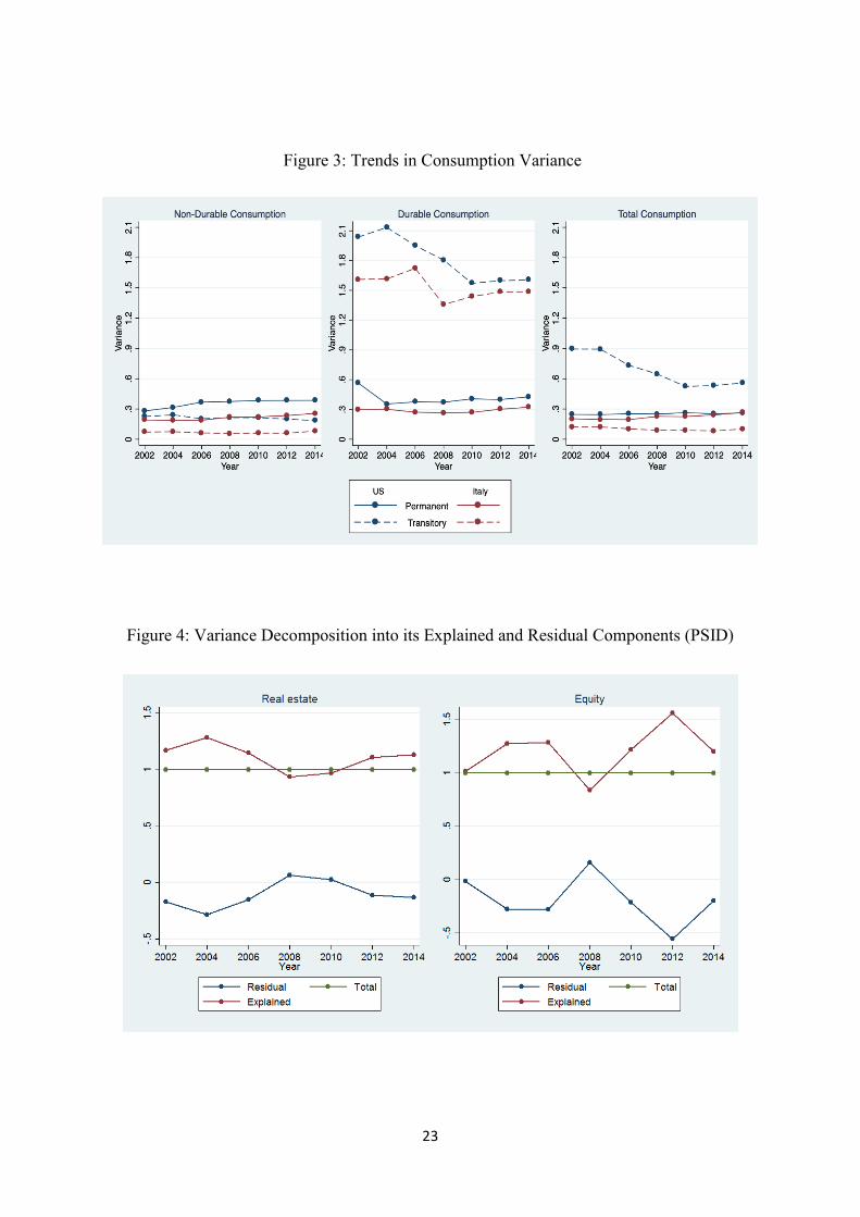
Figure 3 shows results using MG2 with a 5-year moving average window (the other methods

yield qualitatively and quantitatively similar results and the results are available upon request).

The figure shows that, as predicted, when it comes to non-durable consumption, the permanent

component of consumption volatility is higher than the transitory one in both countries. Looking

at consumption volatility of durable goods, instead, we find the opposite results. This is still

12

quite reasonable, as durable goods can be seen as less essential and easier to renounce in case

of adverse economic conditions. What is more surprising is the net effect on total consumption

volatility: while in Italy the narrative of non-durable goods seem to prevail, in the U.S. the

transitory component of consumption volatility matters the most.

4.3 The Effects of the rate of return

On the surface, it seems surprising that wealth volatility is so much greater than income and

consumption volatility, at least for the U.S.. The reason is that an individual’s wealth in year t

depends directly on the person’s wealth in year t-1. The actual equation (for individual 𝑖𝑖) is:

𝑊𝑊𝑖𝑖𝑖𝑖 = 𝑊𝑊𝑖𝑖(𝑖𝑖−1) + 𝑟𝑟𝑖𝑖𝑖𝑖𝑊𝑊𝑖𝑖(𝑖𝑖−1) + 𝑠𝑠𝑖𝑖𝑖𝑖𝑌𝑌𝑖𝑖𝑖𝑖 + 𝐺𝐺𝑖𝑖𝑖𝑖 .

where 𝑊𝑊𝑖𝑖𝑖𝑖 is the net worth at time 𝑡𝑡, 𝑟𝑟 is the rate of return on wealth, 𝑌𝑌𝑖𝑖𝑖𝑖 is income, 𝑠𝑠 represents

the savings rate out of income 𝑌𝑌𝑖𝑖𝑖𝑖, and 𝐺𝐺𝑖𝑖𝑖𝑖 is the net inheritances and gifts received. Changes in

𝑟𝑟, 𝑠𝑠, 𝑌𝑌𝑖𝑖𝑖𝑖, or 𝐺𝐺𝑖𝑖𝑖𝑖 could lead to volatility in wealth over time. However, it is unlikely that 𝑠𝑠 or 𝐺𝐺𝑖𝑖𝑖𝑖

varies too much over time (𝐺𝐺𝑖𝑖𝑖𝑖, in any case, is relatively small). 𝑌𝑌𝑖𝑖𝑖𝑖, on the other hand, does

show some volatility over time, as is evident in Figure 5, though it is smaller than that in 𝑊𝑊𝑖𝑖𝑖𝑖.

Perhaps, the most volatile component is the rate of return 𝑟𝑟. The rate of return faced by an

individual over time depends on both the rate of return for individual assets and the portfolio

composition of assets. The latter is relatively stable over time while rates of return on individual

assets do show a great deal of variation (see Table B1).

To test whether the changes in asset prices do actually explain a significant portion of wealth

volatility, we use rates of return for equity and housing to simulate how these individual wealth

components would evolve if they perfectly followed the market rates of return of the antecedent

period. In order to do so we use country-year data for Italy and the U.S. from the Jordà-

Schularick-Taylor Macrohistory Database,4 which collects a wide range of macroeconomic

variables capturing, among others, asset price dynamics for 17 developed economies between

years 1870 to 2016. We build two-year real return rates based on the annual nominal rates in

4 Accessed on July 23rd 2019.

13

the database and use them to compute the “explained” part of real estate and financial equity.

This allows us to compute an individual “residual” component based on the difference between

the actual value of real estate (equity), as reported in PSID and SHIW, and the explained value

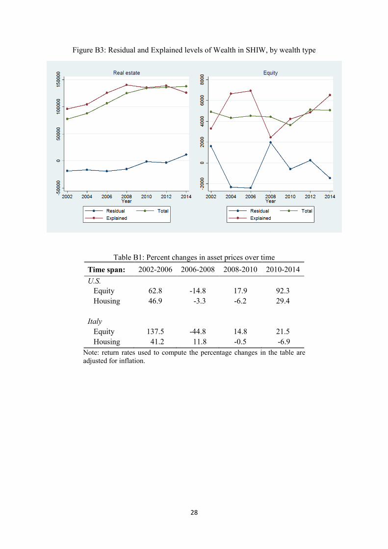
of real estate (equity), based on asset price changes. The decomposition of the levels of housing

and equity into an explained and a residual component for the U.S. and Italy is illustrated

respectively in Figures B2 and B3 of the Appendix. The figures show that housing seems to be

very closely predicted by asset price changes, while changes in equity from year to year are not

explained quite as accurately. This is more so for Italy, partly because the only available

measure of equity in SHIW also includes other financial instruments (such as bills and bonds)

which are impossible to disentangle from financial equity alone.

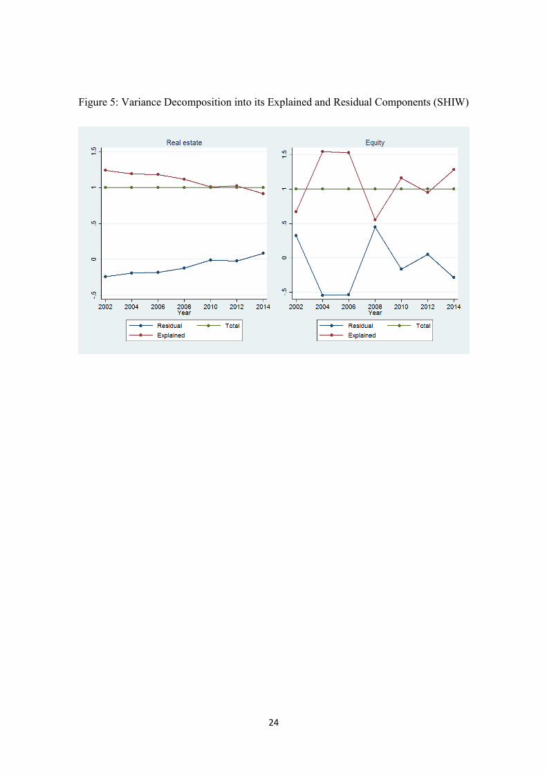
We then test our hypothesis that wealth volatility is in great part driven by the volatility of

returns. Based on the aforementioned decomposition, we assess the contribution of each

component (i.e. explained and residual) to the yearly variances of equity and real estate. We do

so by following Shorrocks’ (1982) decomposition of the variance of income into the

contribution of its factor components. Figure 4 and Figure 5 illustrate the results of this exercise.

In both countries, asset price changes not only fully explain the variance of the value of real

estate, but they tend to systematically overestimate it, such that the residual component of the

variance is negative for almost all years. This appears to hold also for equity, although the

relationship is less stabile across years, especially for Italy (probably due to the measurement

issue mentioned in the paragraph above). Furthermore, both in the U.S. and in Italy (albeit in

the latter only for housing), the portion of the variance explained by asset price changes tends

to reflect more closely the actual variance during the Great Recession with respect to other

years.

5. Heterogeneity analysis

In this section we analyze whether our results on income and wealth volatility are driven by

particular groups of individuals in our samples. In order to do so, we use the transitory

component of the variance derived from the MG1 method. This can in fact be interpreted not

only as the difference between the cross-sectional variance of income and the covariance of

14

current income and one of its past levels, but also as the covariance between current income

and the difference between current income and one of its past levels (the same holds for wealth).

Put more simply,

𝜎𝜎𝜀𝜀𝑖𝑖2 = 𝑉𝑉𝑉𝑉𝑟𝑟(𝑦𝑦𝑖𝑖) − 𝐶𝐶𝐶𝐶𝐶𝐶(𝑦𝑦𝑖𝑖,𝑦𝑦𝑖𝑖−𝑠𝑠) = 𝐶𝐶𝐶𝐶𝐶𝐶(𝑦𝑦𝑖𝑖,𝑦𝑦𝑖𝑖∗)

Where 𝜎𝜎𝜀𝜀𝑖𝑖2 is the MG1 transitory component of the variance and 𝑦𝑦𝑖𝑖∗ ∶= 𝑦𝑦𝑖𝑖 − 𝑦𝑦𝑖𝑖−𝑠𝑠, 𝑠𝑠 < 𝑡𝑡.

In order to assess the contribution of different groups of individuals to the transitory component

of the variances of income and wealth, we decompose the latter by population sub-groups. Let

𝐺𝐺1,𝐺𝐺2, … ,𝐺𝐺𝑘𝑘 be 𝑘𝑘 groups such that every individual in a population of size 𝑁𝑁 belongs to one

(and only one) of the groups, with 𝑘𝑘 ≤ 𝑁𝑁. Let 𝑛𝑛𝑗𝑗 be the size of group 𝐺𝐺𝑗𝑗 and 𝜋𝜋𝑗𝑗 ∶=𝑛𝑛𝑗𝑗𝑁𝑁

the

corresponding population share. It is straightforward then to decompose the covariance between

𝑦𝑦𝑖𝑖 and 𝑦𝑦𝑖𝑖∗ as follows:

𝐶𝐶𝐶𝐶𝐶𝐶(𝑦𝑦𝑖𝑖,𝑦𝑦𝑖𝑖∗) ∶=1𝑁𝑁�(𝑦𝑦𝑖𝑖𝑖𝑖 − 𝑦𝑦�𝑖𝑖)(𝑦𝑦𝑖𝑖𝑖𝑖∗ − 𝑦𝑦�𝑖𝑖∗)𝑁𝑁

𝑖𝑖=1

= �𝜋𝜋𝑗𝑗

𝑘𝑘

𝑗𝑗=1

�1𝑛𝑛𝑗𝑗�(𝑦𝑦𝑖𝑖𝑖𝑖 − 𝑦𝑦�𝑖𝑖)(𝑦𝑦𝑖𝑖𝑖𝑖∗ − 𝑦𝑦�𝑖𝑖∗)𝑖𝑖∈𝐺𝐺𝑗𝑗

�

Where 𝑦𝑦�𝑖𝑖 and 𝑦𝑦�𝑖𝑖∗ are the population averages of 𝑦𝑦𝑖𝑖 and 𝑦𝑦𝑖𝑖∗ respectively. We apply this

decomposition to households in our sample on the basis of available characteristics of the

household itself and household heads. In particular, we use household head’s relationship status

(single or in a cohabiting relationship), gender, age, education, and age. In the U.S. we are also

able to observe the racial group of the household head. We further decompose volatility on the

basis of household size.

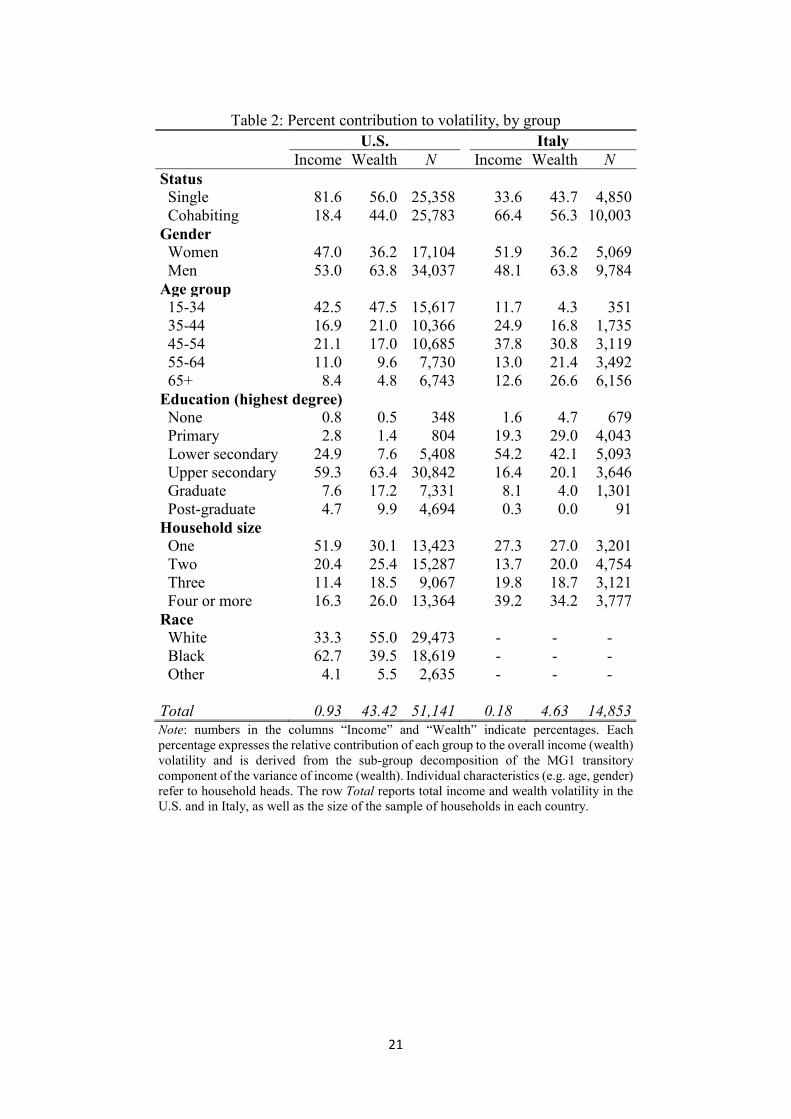
Results are illustrated in Table 2. For each of the two countries, the table reports the percentage

contribution of each sub-group to the overall volatility of income and wealth, as well as the

number of households in each sub-group.5 When it comes to relationship status, cohabitation

seems to have an insulating effect against income and wealth volatility in the U.S., while the

5 Here the overall volatility of income and wealth is computed as the MG1 transitory component of the variance of income and wealth at the household level over the years 2002-2014. Volatility levels for the two countries are reported in the last row of Table 2.

15

opposite is true for Italy. Differences between the two countries appear also when looking at

age of household head: while the share of income and wealth volatility is the highest for young

individuals in the U.S., in Italy it is middle-aged household heads who appear to be the most

vulnerable to income and wealth volatility. Furthermore, individuals in retirement age in the

U.S. do not seem to account for a large share of volatility, which is not the case in Italy –

especially for wealth. Female headed households are less subject to wealth volatility with

respect to male headed and having a graduate or post-graduate degree also seems to have a

dampening effect on both income and wealth volatility. Finally, in the U.S. most of income

volatility can be attributed to households where the head is African-American.

Heterogeneity results shown in Table 2 are robust to the use of other measures of volatility,

such as the variance of the two-year difference in the natural logarithm of income or in the

hyperbolic sine transformation of wealth. The reason we use the variance as a robustness check

instead of the standard deviation is that the former is sub-group decomposable – what we need

in order to disentangle the contribution of different groups of individuals to the sample volatility

of income and wealth. Results for heterogeneity analysis using this other measure of volatility

are available upon request.

6. Conclusions

In this paper we look at the recent trends in income, wealth, and consumption volatility in Italy

and the U.S.. Contrary to what we expected, income volatility is systematically lower than

wealth volatility in both countries. All measures of income and wealth volatility appear to

increase in the aftermath of the financial crisis, with wealth being the most affected, and their

levels are always higher in the U.S. than in Italy. In particular, income volatility in Italy reaches

at most half of the U.S. levels: while partly driven by higher earning inequality in the U.S., this

result could also suggest that the system of tax and transfers in Italy is more efficient in

protecting individuals against income shocks. Consistently with the literature, we also find that

consumption volatility is lower than income volatility and substantially driven by permanent

changes in consumption patterns, although the volatility of durable consumption shows a larger

sensitivity to transitory fluctuations rather than permanent ones. We explain our findings on

16

wealth volatility by looking at how changes in asset prices predict the evolution of individual

wealth in our sample. We find that most of the fluctuations in housing and equity can be

explained by changes in market return rates of these assets.

Our results show that individual wealth in Italy and the U.S. is highly sensitive to year-to-year

fluctuations, largely more so than income. If wealth acts as a buffer to ensure consumption

smoothing over time, protecting individuals against income shocks, then our results are indeed

worrisome – especially in the light of the increasing trend in income volatility. While in this

paper we offer an explanation based on changes in the price of real estate assets and stocks,

other concurrent phenomena are likely to be in place as well. Conley and Glauber (2008) argue

that a reason behind the increased wealth volatility in the U.S. could come from the

liberalization of credit laws in 1978. In fact, between that period and 2004, there was an over

400 percent increase in personal bankruptcy filings in the U.S., most of which were due to

unexpected medical expenses – with individuals covered by medical insurance being affected

as well. The authors argue that other cases were potentially likely to be triggered by trends in

demographic transition, such as increases in family dissolutions. We hope that this paper will

contribute to the debate on income and wealth volatility and that it will stimulate further

research on their interplay, as well as the mechanisms driving these two forces.

17

References

Bartels, C., & Bönke, T. (2010). “German male income volatility 1984 to 2008: trends in

permanent and transitory income components and the role of the welfare state”. SOEPpapers

on Multidisciplinary Panel Data Research, 325. Deutsches Institut für Wirtschaftsforschung

(DIW), Berlin.

Bartels, C., & Bönke, T. (2013). “Can households and welfare states mitigate rising earnings

instability?”. Review of Income and Wealth, 59(2), 250-282.

Boeri, T., & Brandolini, A. (2004). “The age of discontent: Italian households at the beginning

of the decade”. Giornale degli Economisti e Annali di Economia, 63(3-4), 449-487.

Brandolini, A., Cannari, L., d’Alessio, G., & Faiella, I. (2006). “Household wealth distribution

in Italy in the 1990s”. In E.N. Wolff. (Ed.), International Perspectives on Household Wealth

(pp. 225-275). Edward Elgar Publishing.

Conley, D., & Glauber, R. (2008). “Wealth mobility and volatility in black and white”. Center

for American Progress.

Cowell, F. A., & Mercader-Prats, M. (1999). “Equivalence scales and inequality”. In J. Silber

(Ed.), Handbook of Income Inequality Measurement (pp. 405-435). Springer, Dordrecht.

Dagnes, J., Filandri, M., & Storti, L. (2018). “Social class and wealth inequality in Italy over

20 years, 1993–2014”. Journal of Modern Italian Studies, 23(2), 176-198.

Daly, M. C., & Valletta, R. G. (2008). “Cross-national trends in earnings inequality and

instability”. Economics Letters, 99(2), 215-219.

DeBacker, J. M., Heim, B. T., Panousi, V., & Vidangos, I. (2012). “Rising inequality: transitory

or permanent? New evidence from a panel of U.S. tax returns 1987-2006”. Indiana University-

Bloomington: School of Public & Environmental Affairs Research Paper Series, (2011-01), 01.

Diaz-Serrano, L. (2005). “On the negative relationship between labor income uncertainty and

homeownership: Risk-aversion vs. credit constraints”. Journal of Housing Economics, 14(2),

109-126.

Dynan, K., Elmendorf, D., & Sichel, D. (2012). “The evolution of household income volatility”.

BE Journal of Economic Analysis & Policy, 12(2).

18

Fang, W., Miller, S. M., & Yeh, C. C. (2015). “The effect of growth volatility on income

inequality”. Economic Modelling, 45, 212-222.

Feenberg, D., & Coutts, E. (1993). “An introduction to the TAXSIM model”. Journal of Policy

Analysis and management, 12(1), 189-194.

Fisher, J., Johnson, D., Latner, J. P., Smeeding, T., & Thompson, J. (2016). “Inequality and

mobility using income, consumption, and wealth for the same individuals”. RSF: The Russell

Sage Foundation Journal of the Social Sciences, 2(6), 44-58.

Gottschalk, P., & Moffitt, R. A. (1994). “The growth of earnings instability in the U.S. labor

market”. Brookings Papers on Economic Activity, 1994(2), 217-272.

Gottschalk, P., & Moffitt, R. A. (2009). “The rising instability of U.S. earnings”. Journal of

Economic Perspectives, 23(4), 3-24.

Hacker, J. S., & Jacobs, E. (2008). “The Rising Instability of American Family Incomes, 1969-

2004: Evidence from the Panel Study of Income Dynamics”. Economic Policy Institute.Hacker,

J. S. (2019). “The great risk shift: The new economic insecurity and the decline of the American

dream”. Oxford University Press.

Heathcote, J., & Perri, F. (2018). “Wealth and volatility”. Review of Economic Studies, 85(4),

2173-2213.

Jappelli, T., & Pistaferri, L. (2010). “Does consumption inequality track income inequality in

Italy?”. Review of Economic Dynamics, 13(1), 133-153.

Jenkins, S. P. (2011). “Changing fortunes: income mobility and poverty dynamics in Britain”.

OUP Oxford.

Johnson, D. S., & Fisher, J. D. (2018). “Inequality and mobility over the past half century using

income, consumption and wealth.” Paper presented at the ECINEQ 2019 conference.

Jordà, Ò., Knoll, K., Kuvshinov, D., Schularick, M., & Taylor, A. M. (2019). “The rate of return

on everything, 1870–2015”. Quarterly Journal of Economics, 134(3), 1225-1298.

Kimberlin, S., Kim, J., & Shaefer, L. (2014). “An updated method for calculating income and

payroll taxes from PSID data using the NBER’s TAXSIM, for PSID survey years 1999 through

2011”. Unpublished manuscript, University of Michigan.

19

Moffitt, R. A., & Gottschalk, P. (2002). “Trends in the transitory variance of earnings in the

United States”. Economic Journal, 112(478), C68-C73.

Moffitt, R. A., & Gottschalk, P. (2012). “Trends in the transitory variance of male earnings:

methods and evidence”. Journal of Human Resources, 47(1), 204-236.

Moffitt, R. A., & Zhang, S. (2018). “Income volatility and the PSID: past research and new

results” (No. w24390). National Bureau of Economic Research.

Shin, D., & Solon, G. (2011). “Trends in men's earnings volatility: What does the Panel Study

of Income Dynamics show?”. Journal of Public Economics, 95(7-8), 973-982.

Shorrocks, A. F. (1982). “Inequality decomposition by factor components”. Econometrica,

50(1), 193-211.

Stiglitz, J. E. (2012). “Macroeconomic fluctuations, inequality, and human development”.

Journal of Human Development and Capabilities, 13(1), 31-58.

Whalley, J., & Yue, X. (2009). “Rural income volatility and inequality in China”. CESifo

Economic Studies, 55(3-4), 648-668.

Winship, S. R. (2009). “Has there been a great risk shift? Trends in economic instability among

working-age adults”. Harvard University.

Wolff, E. N. (2017). “Household wealth trends in the United States, 1962 to 2016: has middle

class wealth recovered?”. NBER Working Paper No. 24085, November.

20

Tables and Figures

Table 1: Descriptive Statistics for the Estimation Sample Variable Obs. Mean Std. Dev. Min Max Italy Income 32,804 26,639 13,855 1 128,601 Wealth 32,804 194,492 200,362 -6,800 2,250,115 Non-Durable Consumption 32,804 11,779 6,718 719 115,358 Durable Consumption 32,804 1,253 3,537 -20,578 75,607 Assets 32,804 185,571 192,404 0 2,017,615 Year 32,804 2008 3.824 2002 2014 Age 32,804 52 19.023 15 100 Female 32,804 0.52 0.500 0 1 Education

32,804 3.17 0.999 1 6 Household size

32,804 3.04 1.244 1 12 Single woman 32,804 0.15 0.354 0 1 Single man 32,804 0.06 0.238 0 1 U.S. Income 99,413 34,280 23,584 1 24,1567 Wealth 99,413 105,206 226,301 -130,000 3,345,062 Non-Durable Consumption 99,413 9,487 8,726 -255 749,833 Durable Consumption 87,455 29,525 126,056 -26,946 2,453,878 Assets 99,413 62,050 129,874 -329,156 2,758,257 Year 99,413 2008 3.928 2002 2014 Age 99,413 41 17.417 15 101 Female 99,413 0.54 0.499 0 1 Education

91,148 4.11 0.860 1 6 Household size

99,413 3.07 1.563 1 14 Single woman 99,413 0.26 0.437 0 1 Single man 99,413 0.10 0.298 0 1 Race head White 51,141 0.58 0.494 0 1 Black 51,141 0.36 0.481 0 1 Other 51,141 0.05 0.221 0 1 Race spouse White 25,901 0.71 0.454 0 1 Black 25,901 0.21 0.410 0 1 Other 25,901 0.07 0.248 0 1

Note: all monetary mesures are equivalised and expressed in 2010 constant dollars.

21

Table 2: Percent contribution to volatility, by group

U.S. Italy Income Wealth N Income Wealth N Status Single 81.6 56.0 25,358 33.6 43.7 4,850 Cohabiting 18.4 44.0 25,783 66.4 56.3 10,003 Gender

Women 47.0 36.2 17,104 51.9 36.2 5,069 Men 53.0 63.8 34,037 48.1 63.8 9,784 Age group

15-34 42.5 47.5 15,617 11.7 4.3 351 35-44 16.9 21.0 10,366 24.9 16.8 1,735 45-54 21.1 17.0 10,685 37.8 30.8 3,119 55-64 11.0 9.6 7,730 13.0 21.4 3,492 65+ 8.4 4.8 6,743 12.6 26.6 6,156 Education (highest degree) None 0.8 0.5 348 1.6 4.7 679 Primary 2.8 1.4 804 19.3 29.0 4,043 Lower secondary 24.9 7.6 5,408 54.2 42.1 5,093 Upper secondary 59.3 63.4 30,842 16.4 20.1 3,646 Graduate 7.6 17.2 7,331 8.1 4.0 1,301 Post-graduate 4.7 9.9 4,694 0.3 0.0 91 Household size

One 51.9 30.1 13,423 27.3 27.0 3,201 Two 20.4 25.4 15,287 13.7 20.0 4,754 Three 11.4 18.5 9,067 19.8 18.7 3,121 Four or more 16.3 26.0 13,364 39.2 34.2 3,777 Race

White 33.3 55.0 29,473 - - - Black 62.7 39.5 18,619 - - - Other 4.1 5.5 2,635 - - - Total 0.93 43.42 51,141 0.18 4.63 14,853 Note: numbers in the columns “Income” and “Wealth” indicate percentages. Each percentage expresses the relative contribution of each group to the overall income (wealth) volatility and is derived from the sub-group decomposition of the MG1 transitory component of the variance of income (wealth). Individual characteristics (e.g. age, gender) refer to household heads. The row Total reports total income and wealth volatility in the U.S. and in Italy, as well as the size of the sample of households in each country.

22

Figure 1: Trends in Transitory and Permanent Income Variance

Figure 2: Trends in Transitory and Permanent Wealth Variance

23

Figure 3: Trends in Consumption Variance

Figure 4: Variance Decomposition into its Explained and Residual Components (PSID)

24

Figure 5: Variance Decomposition into its Explained and Residual Components (SHIW)

25

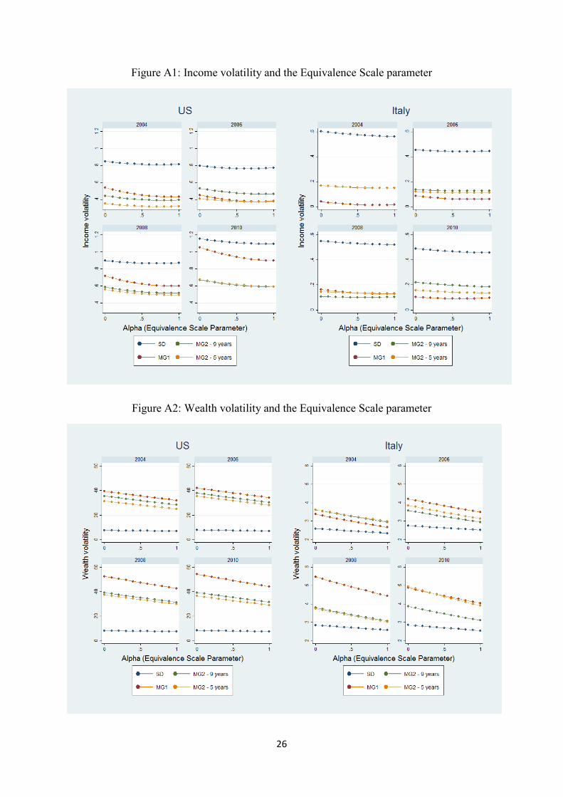
Appendix A: Volatility and the Equivalence Scale Parameter

We here look at the sensitivity of our volatility measures to the choice of the equivalisation

parameter α.6 In Figure A1 and Figure A2 we plot the relationship between income and wealth

volatility and the parameter for the years in which all of our volatility measures were available,

namely 2004, 2006, 2008, and 2010. Depending on the measure used and on the year

considered, we find either a U-shaped or a negative relationship between income volatility and

α. This is consistent with the considerations on income inequality and the equivalence scale

parameter by Cowell and Mercader-Prats (1999), who find a similar U-shaped relationship

using Spanish data. The measure that seems to be the most sensitive to the choice of α,

especially in the U.S., is the transitory component of the income variance derived with the MG1

method. We find a flatter relationship instead for other measures, especially the standard

deviation.

Figure A2 shows a linear relationship (with negative slope) between wealth volatility and the

equivalisation parameter. This comes as no surprise, since by construction there is an

approximately linear relationship between the inverse hyperbolic sine transformation we used

to rescale equivalised household wealth and the equivalisation parameter. Again, the measure

that appears to be less sensitive to the choice of α is the standard deviation of the individual

percentage changes in wealth between two consecutive periods (SD in the Figures).

6 The parametric equivalence scale we use divides household income (wealth) by the number of household members raised to the parameter α, 𝛼𝛼 ∈ [0,1].

26

Figure A1: Income volatility and the Equivalence Scale parameter

Figure A2: Wealth volatility and the Equivalence Scale parameter

27

Appendix B: Other Figures and Tables

Figure B1: Income and Wealth volatility in Italy and the U.S.

Figure B2: Residual and Explained levels of Wealth in PSID, by wealth type

28

Figure B3: Residual and Explained levels of Wealth in SHIW, by wealth type

Table B1: Percent changes in asset prices over time

Time span: 2002-2006 2006-2008 2008-2010 2010-2014 U.S. Equity 62.8 -14.8 17.9 92.3 Housing 46.9 -3.3 -6.2 29.4 Italy Equity 137.5 -44.8 14.8 21.5 Housing 41.2 11.8 -0.5 -6.9

Note: return rates used to compute the percentage changes in the table are adjusted for inflation.