Income and Substitution Effects in Consumer Goods Markets · 1Chapters 2 and 4 through 6 are...

We have just demonstrated in Chapter 6 how we can use our model of choice sets and tastes toillustrate optimal decision making by individuals such as consumers or workers.1 We now turn tothe question of how such optimal decisions change when economic circumstances change. Sinceeconomic circumstances in this model are fully captured by the choice set, we could put this dif-ferently by saying that we will now ask how optimal choices change when income, endowments,or prices change.

As we proceed, it is important for us to keep in mind the difference between tastes and behav-ior. Behavior, or what we have been calling choice, emerges when tastes confront circumstancesas individuals try to do the “best” they can given those circumstances. If I buy less wine becausethe price of wine has increased, my behavior has changed but my tastes have not. Wine still tastesthe same as it did before, it just costs more. In terms of the tools we have developed, my indiffer-ence map remains exactly as it was. I simply move to a different indifference curve as my circum-stances (i.e., the price of wine) change.

In the process of thinking about how behavior changes with economic circumstances, we willidentify two conceptually distinct causes, known as income and substitution effects.2 At first itwill seem like the distinction between these effects is abstract and quite unrelated to real-worldissues we care about. As you will see later, however, this could not be further from the truth. Deepquestions related to the efficiency of tax policy, the effectiveness of Social Security and healthpolicy, and the desirability of different types of antipoverty programs are fundamentally rooted inquestions related to income and substitution effects. While we are still in the stage of buildingtools for economic analysis, I hope you will be patient and bear with me as we develop an under-standing of these tools.

Still, it may be useful to at least give an initial example to motivate the effects we will develop inthis chapter, an example that will already be familiar to you if you have done end-of-chapter exercise6.14. As you know, there is increasing concern about carbon-based emissions from automobiles, andan increased desire by policy makers to find ways of reducing such emissions. Many economistshave long recommended the simple policy of taxing gasoline heavily in order to encourage con-sumers to find ways of conserving gasoline (by driving less and buying more fuel-efficient cars). Theobvious concern with such a policy is that it imposes substantial hardship on households that rely

110

C H A P T E R

7Income and SubstitutionEffects in Consumer Goods Markets

1Chapters 2 and 4 through 6 are required reading for this chapter. Chapter 3 is not necessary. 2This distinction was fully introduced into neoclassical economics by Sir John Hicks in his influential book, Value and Capital,originally published in 1939. Hicks was awarded the Nobel Prize in Economics in 1972 (together with Ken Arrow).

74707_07_ch07_p110-128.qxd 12/23/09 4:20 PM 10

Chapter 7. Income and Substitution Effects in Consumer Goods Markets 111

heavily on their cars, particularly poorer households that would be hit pretty hard by such a tax. Someeconomists have therefore proposed simply sending all tax revenues from such a gasoline tax back totaxpayers in the form of a tax refund. This has led many editorial writers to conclude that economistsmust be nuts; after all, if we send the money back to the consumers, wouldn’t they then just buy thesame amount of gasoline as before since (at least on average) they would still be able to afford it?Economists may be nuts, but our analysis will tell us that they are also almost certainly right, and edi-torial writers are almost certainly wrong, when it comes to the prediction of how this policy proposalwould change behavior. And the explanation lies fully in an understanding of substitution effects thateconomists understand and most noneconomists don’t think about. We’ll return to this in the conclu-sion to the chapter.

As we have seen in Chapters 2 and 3, there are two primary ways in which choice sets (and thusour economic circumstances) can change: First, a change in our income or wealth might shiftour budget constraints without changing their slopes, and thus without changing the opportu-nity costs of the various goods we consume. Second, individual prices in the economy—whether in the form of prices of goods, wages, or interest rates—may change and thus alter theslopes of our budget constraints and the opportunity costs we face. These two types of changesin choice sets result in different types of effects on behavior, and we will discuss them sepa-rately in what follows. First, we will look only at what happens to economic choices whenincome or wealth changes without a change in opportunity costs (Section 7.1). Next, we willinvestigate how decisions are impacted when only opportunity costs change without a changein real wealth (Section 7.2). Finally, we will turn to an analysis of what happens when changesin income and opportunity costs occur at the same time, which, as it turns out, is typically thecase when relative prices in the economy change.

7.1 The Impact of Changing Income on Behavior

What happens to our consumption when our income increases because of a pay raise at work orwhen our wealth endowment increases because of an unexpected inheritance or when our leisureendowment rises due to the invention of some time-saving technology? Would we consume moreshirts, pants, Coke, housing, and jewelry? Would we consume more of some goods and fewer ofothers, work more or less, save more or less? Would our consumption of all goods go up by thesame proportion as our income or wealth?

The answer depends entirely on the nature of our tastes, and the indifference map that repre-sents our tastes. For most of us, it is likely that our consumption of some goods will go up by alot while our consumption of other goods will increase by less, stay the same, or even decline.The impact of changes in our income or wealth on our consumption decisions (in the absence ofchanges in opportunity costs) is known as the income or wealth effect.

The economics “lingo” is not entirely settled on whether to call this kind of an effect a“wealth” or an “income” effect, and we will use the two terms in the following way: Wheneverwe are analyzing a model where the size of the choice set is determined by exogenously givenincome, as in Chapter 2 and for the remainder of this chapter, we will refer to the impact of achange in income as an income effect. In models where the size of the choice set is determined bythe value of an endowment, as in Chapter 3 and in the next chapter, we will refer to the impact ofchanges in that endowment as a wealth effect. What should be understood throughout, however,is that by both income and wealth effect we mean an impact on consumer decisions that arisesfrom a parallel shift in the budget constraint, a shift that does not include a change in opportunitycosts as captured by a change in the slope of the budget line.

7.1.1 Normal and Inferior Goods During my first few years in graduate school, my wife andI made relatively little money. Often, our budget would permit few extravagances, with dinners

74707_07_ch07_p110-128.qxd 12/23/09 4:20 PM Page 111

112 Part 1. Utility-Maximizing Choice: Consumers, Workers, and Savers

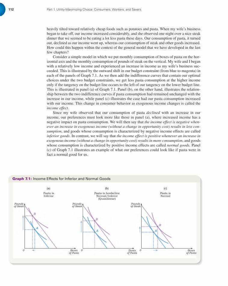
Graph 7.1: Income Effects for Inferior and Normal Goods

heavily tilted toward relatively cheap foods such as potatoes and pasta. When my wife’s businessbegan to take off, our income increased considerably, and she observed one night over a nice steakdinner that we seemed to be eating a lot less pasta these days. Our consumption of pasta, it turnedout, declined as our income went up, whereas our consumption of steak and other goods increased.How could this happen within the context of the general model that we have developed in the lastfew chapters?

Consider a simple model in which we put monthly consumption of boxes of pasta on the hor-izontal axis and the monthly consumption of pounds of steak on the vertical. My wife and I beganwith a relatively low income and experienced an increase in income as my wife’s business suc-ceeded. This is illustrated by the outward shift in our budget constraint (from blue to magenta) ineach of the panels of Graph 7.1. As we then add the indifference curves that contain our optimalchoices under the two budget constraints, we get less pasta consumption at the higher incomeonly if the tangency on the budget line occurs to the left of our tangency on the lower budget line.This is illustrated in panel (a) of Graph 7.1. Panel (b), on the other hand, illustrates the relation-ship between the two indifference curves if pasta consumption had remained unchanged with theincrease in our income, while panel (c) illustrates the case had our pasta consumption increasedwith our income. This change in consumer behavior as exogenous income changes is called theincome effect.

Since my wife observed that our consumption of pasta declined with an increase in ourincome, our preferences must look more like those in panel (a), where increased income has anegative impact on pasta consumption. We will then say that the income effect is negative when-ever an increase in exogenous income (without a change in opportunity cost) results in less con-sumption, and goods whose consumption is characterized by negative income effects are calledinferior goods. In contrast, we will say that the income effect is positive whenever an increase inexogenous income (without a change in opportunity cost) results in more consumption, and goodswhose consumption is characterized by positive income effects are called normal goods. Panel(c) of Graph 7.1 illustrates an example of what our preferences could look like if pasta were infact a normal good for us.

74707_07_ch07_p110-128.qxd 12/23/09 4:20 PM Page 112


Finally, panel (b) of Graph 7.1 illustrates an indifference map that gives rise to no incomeeffect on our pasta consumption. Notice the following defining characteristic of this indifferencemap: The marginal rate of substitution is constant along the vertical line that connects points and . In Chapter 5, we called tastes that are represented by indifference curves whose marginalrates of substitution are constant in this way quasilinear (in pasta). The sequence of panels inGraph 7.1 then illustrates how quasilinear tastes are the only kinds of tastes that do not give riseto income effects for some good, and as such they represent the borderline case between normaland inferior goods.

It is worthwhile noting that whenever we observe a negative income effect on our consump-tion of one good, there must be a positive income effect on our consumption of a different good.After all, the increased income must be going somewhere, whether it is increased consumptionof some good today or increased savings for consumption in the future. In Graph 7.1a, forinstance, we observe a negative income effect on our consumption of pasta on the horizontalaxis. At the same time, on the vertical axis we observe a positive income effect on our consump-tion of steak.

BA

7.1.2 Luxuries and Necessities As we have just seen, quasilinear tastes represent onespecial case that divides two types of goods: normal goods whose consumption increases withincome and inferior goods whose consumption decreases with income. The defining differencebetween these two types of goods is how consumption changes in an absolute sense as ourincome changes. A different way of dividing goods into two sets is to ask how our relativeconsumption of different goods changes as income changes. Put differently, instead of askingwhether total consumption of a particular good increases or decreases with an increase inincome, we could ask whether the fraction of our income spent on a particular good increasesor decreases as our income goes up; i.e., whether our consumption increases relative toour income.

Consider, for instance, our consumption of housing. In each panel of Graph 7.2, wemodel choices between square footage of housing and “dollars of other goods.” As in the pre-vious graph, we consider how choices will change as income doubles, with bundle repre-senting the optimal choice at the lower income and bundle representing the optimal choiceat the higher income. Suppose that in each panel, the individual spends 25% of her incomeon housing at bundle . If housing remains a constant fraction of consumption as incomeincreases, then the optimal consumption bundle when income doubles would simplyinvolve twice as much housing and twice as much “other good” consumption. This bundlewould then lie on a ray emanating from the origin and passing through point , as pictured inGraph 7.2b. If, on the other hand, the fraction of income allocated to housing declines asincome rises, would lie to the left of this ray (as in Graph 7.2a), and if the fraction ofincome allocated to housing increases as income rises, would lie to the right of the ray (asin Graph 7.2c). It turns out that on average, people spend approximately 25% of their incomeon housing regardless of how much they make, which implies that tastes for housing typi-cally look most like those in Graph 7.2b.

BB

A

BA

BA

Is it also the case that whenever there is a positive income effect on our consumption of onegood, there must be a negative income effect on our consumption of a different good?

Exercise7A.1

Can a good be an inferior good at all income levels? (Hint: Consider the bundle (0,0).) Exercise7A.2

74707_07_ch07_p110-128.qxd 12/23/09 4:20 PM Page 113


Graph 7.2: Income Effects for Necessities and Luxuries

Economists have come to refer to goods whose consumption as a fraction of income declineswith income as necessities while referring to goods whose consumption as a fraction of incomeincreases with income as luxuries. The borderline tastes that divide these two classes of goods aretastes of the kind represented in Graph 7.2b, tastes that we defined as homothetic in Chapter 5.(Recall that we said tastes were homothetic if the marginal rates of substitution are constant alongany ray emanating from the origin.) Thus, just as quasilinear tastes represent the borderline tastesbetween normal and inferior goods, homothetic tastes represent the borderline tastes betweennecessary and luxury goods.

7.2 The Impact of Changing Opportunity Costs on Behavior

Suppose my brother and I go off on a week-long vacation to the Cayman Islands during dif-ferent weeks. He and I are identical in every way, same income, same tastes.3 Since there isno public transportation on the Cayman Islands, you only have two choices of what to do onceyou step off the airplane: you can either rent a car for the week, or you can take a taxi to yourhotel and then rely on taxis for any additional transportation needs. After we returned homefrom our respective vacations, we compared notes and discovered that, although we hadstayed at exactly the same hotel, I had rented a car whereas my brother had used only taxis.

3This assumption is for illustration only. Both my brother and I are horrified at the idea of anyone thinking we are identical, andhe asked for this clarification in this text.

Exercise7A.3

Are all inferior goods necessities? Are all necessities inferior goods? (Hint: The answer to the firstis yes; the answer to the second is no.) Explain.

Exercise7A.4

At a particular consumption bundle, can both goods (in a two-good model) be luxuries? Can theyboth be necessities?

74707_07_ch07_p110-128.qxd 12/23/09 4:20 PM Page 114


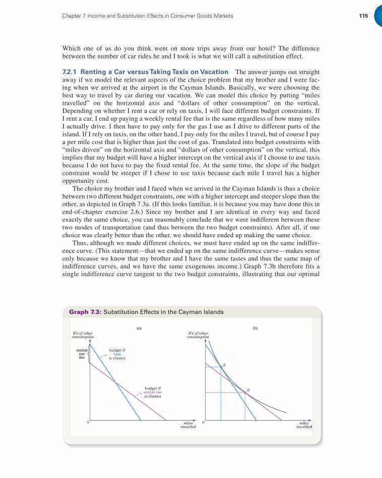
Graph 7.3: Substitution Effects in the Cayman Islands

Which one of us do you think went on more trips away from our hotel? The differencebetween the number of car rides he and I took is what we will call a substitution effect.

7.2.1 Renting a Car versus Taking Taxis on Vacation The answer jumps out straightaway if we model the relevant aspects of the choice problem that my brother and I were fac-ing when we arrived at the airport in the Cayman Islands. Basically, we were choosing thebest way to travel by car during our vacation. We can model this choice by putting “milestravelled” on the horizontal axis and “dollars of other consumption” on the vertical.Depending on whether I rent a car or rely on taxis, I will face different budget constraints. IfI rent a car, I end up paying a weekly rental fee that is the same regardless of how many milesI actually drive. I then have to pay only for the gas I use as I drive to different parts of theisland. If I rely on taxis, on the other hand, I pay only for the miles I travel, but of course I paya per mile cost that is higher than just the cost of gas. Translated into budget constraints with“miles driven” on the horizontal axis and “dollars of other consumption” on the vertical, thisimplies that my budget will have a higher intercept on the vertical axis if I choose to use taxisbecause I do not have to pay the fixed rental fee. At the same time, the slope of the budgetconstraint would be steeper if I chose to use taxis because each mile I travel has a higheropportunity cost.

The choice my brother and I faced when we arrived in the Cayman Islands is thus a choicebetween two different budget constraints, one with a higher intercept and steeper slope than theother, as depicted in Graph 7.3a. (If this looks familiar, it is because you may have done this inend-of-chapter exercise 2.6.) Since my brother and I are identical in every way and facedexactly the same choice, you can reasonably conclude that we were indifferent between thesetwo modes of transportation (and thus between the two budget constraints). After all, if onechoice was clearly better than the other, we should have ended up making the same choice.

Thus, although we made different choices, we must have ended up on the same indiffer-ence curve. (This statement—that we ended up on the same indifference curve—makes senseonly because we know that my brother and I have the same tastes and thus the same map ofindifference curves, and we have the same exogenous income.) Graph 7.3b therefore fits asingle indifference curve tangent to the two budget constraints, illustrating that our optimal

74707_07_ch07_p110-128.qxd 12/23/09 4:20 PM Page 115


choices on the two different budget constraints result in the same level of satisfaction. Mybrother’s optimal choice then indicates fewer miles travelled than my optimal choice .

The intuition behind the model’s prediction is straightforward. Once I sped off to my hotel inmy rented car, I had to pay the rental fee no matter what else I did for the week. So, the opportu-nity cost or price of driving a mile (once I decided to rent a car) was only the cost of gasoline. Mybrother, on the other hand, faced a much higher opportunity cost since he had to pay taxi pricesfor every mile he travelled. Even though our choices made us equally well off, it is clear that mylower opportunity cost of driving led me to travel more miles and consume less of other goodsthan my brother.

BA

Economists will often say that the flat weekly rental fee becomes a sunk cost as soon as I havechosen to rent a car. Once I have rented the car, there is no way for me to get back the fixed rentalfee that I have agreed to pay, and it stays the same no matter what I do once I leave the rental carlot. So, the rental fee is never an opportunity cost of anything I do once I have rented the car. Suchsunk costs, once they have been incurred, therefore do not affect economic decisions because oureconomic decisions are shaped by the trade-offs inherent in opportunity costs. We will return tothe concept of sunk costs more extensively when we discuss producer behavior, and we will notein Chapter 29 that some psychologists quarrel with the economist’s conclusion that such costsshould have no impact on behavior.

7.2.2 Substitution Effects The difference in my brother’s and my behavior in our CaymanIsland example is what is known as a substitution effect. Substitution effects arise wheneveropportunity costs or prices change. In our example, for instance, we analyzed the difference inconsumer behavior when the price of driving changes, but the general intuition behind the substi-tution effect will be important for many more general applications throughout this book.

We will define a substitution effect more precisely as follows: The substitution effect of a pricechange is the change in behavior that results purely from the change in opportunity costs and notfrom a change in real income. By real income, we mean real welfare, so “no change in real income”should be taken to mean “no change in satisfaction” or “no change in indifference curves.” TheCayman Island example was constructed so that we could isolate a substitution effect clearly byfocusing our attention on a single indifference curve or a single level of “real income.”4

The fact that bundle must lie to the right of bundle is a simple matter of geometry: Asteeper budget line fit tangent to an indifference curve must lie to the left of a shallower budgetline that is tangent to the same indifference curve. The direction of a substitution effect is there-fore always toward more consumption of the good that has become relatively cheaper and awayfrom the good that has become relatively more expensive. Note that this differs from what weconcluded about income effects whose direction depends on whether a good is normal or inferior.

7.2.3 How Large Are Substitution Effects? While the direction of substitution effectsis unambiguous, the size of the effect is dependent entirely on the kinds of underlying tastes aconsumer has. The picture in Graph 7.3b suggests a pretty clear and sizable difference between

AB

4This definition of “real income” differs from another definition you may run into during your studies of economics (one thatwe also used in an earlier chapter on budget constraints). Macroeconomists who study inflation, or microeconomists whowant to study behavior that is influenced by inflation, often define “real income” as “inflation adjusted income.” For instance,when comparing someone’s income in 1990 to his or her income in 2000, an economist might adjust the 2000 income by theamount of inflation that occurred between 1990 and 2000, thus reporting 2000 “real income” expressed in 1990 dollars.

Exercise7A.5

If you knew only that my brother and I had the same income (but not necessarily the sametastes), could you tell which one of us drove more miles: the one that rented or the one thattook taxis?

74707_07_ch07_p110-128.qxd 12/23/09 4:20 PM Page 116


Graph 7.4: The Degree of Substitutability and the Size of Substitution Effects

the number of miles I drove and the number of miles my brother drove given that we faceddifferent opportunity costs for driving while having the same level of satisfaction or welfare.But I could have equally well drawn the indifference curve with more curvature, and thus withless substitutability between miles driven and other consumption. The less substitutability isbuilt into a consumer’s tastes, the smaller will be substitution effects arising from changes inopportunity costs.

For instance, consider the indifference curve in Graph 7.4b, an indifference curve with morecurvature than that in Graph 7.4a and thus less built-in substitutability along the portion on whichmy brother and I are making our choices. Notice that, although the substitution effect points inthe same direction as before, the effect is considerably smaller. Graph 7.4c illustrates the roleplayed by the level of substitutability between goods even more clearly by focusing on theextreme case of perfect complements. Such tastes give rise to indifference curves that permit nosubstitutability between goods, leading to bundles and overlapping and a consequent disap-pearance of the substitution effect.

BA

7.2.4 “Hicks” versus “Slutsky” Substitution We have now defined the substitutioneffect as the change in consumption that is due to a change in opportunity cost without a changein “‘real income”; i.e., without a change in the indifference curve. This is sometimes calledHicksian substitution. A slightly different concept of a substitution effect arises when we ask howa change in opportunity costs alters a consumer’s behavior assuming that her ability to purchasethe original bundle remains intact. This is called Slutsky substitution. It operates very similarly toHicksian substitution, and we will therefore leave it to end-of-chapter exercise 7.11 to explorethis further. We are also using the idea in exercise 7.11 (and its previous companion exercise6.16) and 7.6 (as well as its previous companion exercise 6.9).

True or False: If you observed my brother and me consuming the same number of miles drivenduring our vacations, then our tastes must be those of perfect complements between milesdriven and other consumption.

Exercise7A.6

74707_07_ch07_p110-128.qxd 12/23/09 4:20 PM Page 117


Graph 7.5: Income and Substitution Effects when Gasoline Is a Normal Good

7.3 Price Changes: Income and Substitution Effects Combined

As you were reading through the Cayman Island example, you may have wondered why I chosesuch an admittedly contrived story. The reason is that I wanted to follow our discussion of pureincome effects (which occur in the absence of changes in opportunity costs) in Section 7.1 witha discussion of pure substitution effects (which occur in the absence of any changes in realincome or wealth) in Section 7.2. Most real-world changes in opportunity costs, however, implic-itly also give rise to changes in real income, causing the simultaneous operation of both incomeand substitution effects.

Let’s forget the Cayman Islands, then, and consider what happens when the price of a goodthat most of us consume goes up, as, for instance, the price of gasoline. When this happens, I canno longer afford to reach the same indifference curve as before if my exogenous income remainsthe same. Thus, not only do I face a different opportunity cost for gasoline but I also have to facethe prospect of ending up with less satisfaction—or what we have called less “real” income—because I am doomed to operate on a lower indifference curve than before the price increase.Similarly, if the price of gasoline declines, I not only face a different opportunity cost for gaso-line but will also end up on a higher indifference curve, and thus experience an increase in realincome. A price change therefore typically results in both an income effect and a substitutioneffect. These can be conceptually disentangled even though they occur simultaneously, and it willbecome quite important for many policy applications to know the relative sizes of these concep-tually different effects. You will see how this is important more clearly in later chapters. For now,we will simply focus on conceptually disentangling the two effects of price changes.

7.3.1 An Increase in the Price of Gasoline To model the impact of an increase in the price ofgasoline on my behavior, we can once again put “miles driven” on the horizontal axis and “dollars ofother consumption” on the vertical. An increase in the price of gasoline then causes an inward rota-tion of the budget line around the vertical intercept, as illustrated in Graph 7.5a. My optimal bundleprior to the price increase is illustrated by the tangency of the indifference curve at point .A

74707_07_ch07_p110-128.qxd 12/23/09 4:20 PM Page 118


We can now begin our disentangling of income and substitution effects by asking how myconsumption bundle would have changed had I only experienced the change in opportunity costswithout a change in my real income. Put differently, we can ask how my consumption decisionwould change if I faced a new budget that incorporated the steeper slope implied by the pricechange but was large enough to permit me to be as satisfied as I was before the price change, largeenough to keep me on my original indifference curve. This budget is illustrated as the greenbudget tangent to the indifference curve containing bundle A in Graph 7.5b and is called the com-pensated budget. A compensated budget for a price change is the budget that incorporates thenew price but includes sufficient monetary compensation to make the consumer as well off as shewas before the price change. If income is exogenous (as it is in our example), the compensatedbudget requires positive compensation when prices increase and negative compensation whenprices decrease.

Graph 7.5b then looks very much like Graph 7.4b that illustrated a pure substitution effect forour Cayman Islands example. This is because we have imagined that I was provided sufficient com-pensation at the higher gasoline price to keep my real income constant in order to focus only on thechange in my consumption that is due to the change in my opportunity costs along a single indiffer-ence curve. As in the Cayman example, we can then quickly see that consumption of gasoline is lessat point than at point . When real income is unchanged, the substitution effect tells us that I willconsume less gasoline because gasoline has become more expensive relative to other goods.

Rarely, however, will someone come to me and offer me compensation for a price change in reallife. Rather, I will have to settle for a decrease in my real income when prices go up. In Graph 7.5c,we thus start with the compensated budget and ask how my actual consumption decision will differfrom the hypothetical outcome . Before answering this question, notice that the compensatedbudget and the final budget in Graph 7.5c have the same slope and thus differ only by the hypothet-ical compensation we have assumed when plotting the compensated budget. Thus when going fromthe compensated (green) to the final (magenta) budget, we are simply analyzing the impact of achange in my exogenous money income, or what we called a pure income effect in Section 7.1.

Whether my optimal consumption of gasoline on my final budget line is larger or smaller thanat point then depends entirely on whether gasoline is a normal or an inferior good for me. Wedefined a normal good as one whose consumption moves in the same direction as changes inexogenous income, while we defined an inferior good as one whose consumption moved in theopposite direction of changes in exogenous income. Thus, the optimal bundle on the final budgetmight lie to the left of point if gasoline is a normal good, and it might lie to the right of ifgasoline is an inferior good. In the latter case, it could lie in between and if the income effectis smaller than the substitution effect, or it might lie to the right of point if the income effect islarger than the substitution effect. In Graph 7.5c, we illustrate the case where gasoline is a nor-mal good, and the optimal final bundle lies to the left of . In this case, both income and sub-stitution effects suggest that I will purchase less gasoline as the price of gasoline increases.

7.3.2 Regular Inferior and Giffen Goods Notice that we can conclude unambiguouslythat my consumption of gasoline will decline if its price increases whenever gasoline is a normalgood (as is the case if bundle in Graph 7.5c is my optimal final choice). This is because both thesubstitution and the income effect suggest declining consumption. If, on the other hand, gasolineis an inferior good for me, then my gasoline consumption could increase or decrease dependingon whether my final consumption bundle lies between and as in Graph 7.6a or whether it liesto the right of as in Graph 7.6b. We can therefore divide inferior goods into two subcategories:those whose consumption decreases with an increase in price and those whose consumptionincreases with an increase in price (when exogenous income remains constant). We will call theformer regular inferior goods and the latter Giffen goods.

When initially introduced to the possibility that a consumer might purchase more of a goodwhen its price goes up, students often misinterpret what economists mean by this. A commonexample that students will think of is that of certain goods that carry a high level of prestige

ABA

C

BC

ABA

BB

B

B

AB

74707_07_ch07_p110-128.qxd 12/23/09 4:20 PM Page 119


precisely because everyone knows they are expensive. For instance, it may be true that some con-sumers who care about the prestige value of a BMW will be more likely to purchase BMWs asthe price (and thus the prestige value) increases. This is not, however, the kind of behavior wehave in mind when we think of Giffen goods. The person who attaches a prestige value to theprice of a BMW is really buying two different goods when he or she buys this car: the car itselfand the prestige value of the car. As the price of the BMW goes up, the car remains the same butthe quantity of prestige value rises. So, a consumer who is more likely to buy BMWs as the priceincreases is not buying more of a single good but is rather buying a different mix of goods whenthe price of the BMW goes up. When the same consumer’s income falls (and the price of BMWsremains the same), the consumer would almost certainly be less likely to buy BMWs, which indi-cates that the car itself (with the prestige value held constant) is a normal good.5

Real Giffen goods are quite different, and we rarely observe them in the real world.Economists have struggled for literally centuries to find examples; this is how rare they are. Atthe end of the 19th century, Alfred Marshall (1842–1924), one of the great economists of thatcentury, included a hypothetical example in his economics textbook and attributed it to RobertGiffen, a contemporary of his.6 Over the years, a variety of attempts to find credible historicalexamples that are not hypothetical have been discredited, although a recent paper demonstratesthat rice in poor areas of China may indeed be a Giffen good there.7

5While an increase in the price still causes an increase in the consumption of the physical good we observe, such goods areexamples of what is known as Veblen Goods after Thorstein Veblen (1857–1929) who hypothesized that preferences for cer-tain goods intensify as price increases, which can cause what appear to be increases in consumption as price goes up. Youcan think through this more carefully in end-of-chapter exercise 7.9, where you are asked to explain an increase in the con-sumption of Gucci accessories when the price increases. In Chapter 21, we revisit Veblen goods in end-of-chapter exercise21.5 in the context of network externalities.6To quote from his text: “As Mr. Giffen has pointed out, a rise in the price of bread makes so large a drain on the resources ofthe poorer labouring families . . . that they are forced to curtail their consumption of meat and the more expensive farinaceousfoods: and bread being still the cheapest food which they can get and will take, they consume more, and not less of it.” A.Marshall, Principles of Economics (MacMillan: London, 1895). While Robert Giffen (1837–1910) was a highly regarded econo-mist and statistician, it appears no one has located a reference to the kinds of goods that are named after him in any of hisown writings, only in Marshall’s.7R. Jensen and N. Miller, (2007). “Giffen Behavior: Theory and Evidence,” National Bureau of Economic Research workingpaper 13243 (Cambridge, MA, 2007).

Graph 7.6: Income and Substitution Effects When Gasoline Is an Inferior Good

74707_07_ch07_p110-128.qxd 12/23/09 4:20 PM Page 120


A friend of mine in graduate school once told me a story that is the closest example I have everpersonally heard of a real Giffen good. He came from a relatively poor family in the Midwest wherewinters get bitterly cold and where they heated their home with a form of gasoline. Every winter, theywould spend a month over Christmas with relatives in Florida. One year during the 1973 energy cri-sis, the price of gasoline went up so much that they decided they could not afford to go on theirannual vacation in Florida. So, they stayed in the Midwest and had to heat their home for one addi-tional month. While they tried to conserve on gasoline all winter, they ended up using more thanusual because of that extra month. Thus, their consumption of gasoline went up precisely because theprice of gasoline went up and the income effect outweighed the substitution effect. This example, aswell as the recent research on rice in China, both illustrate that, in order to find the “Giffen behavior”of increasing consumption with an increase in price, it must be that the good in question represents alarge portion of a person’s income to begin with, with a change in price therefore causing a largeincome effect. It furthermore must be the case that there are no very good substitutes for the good inorder for the substitution effect to remain small. Given the variety of substitutable goods in the mod-ern world and the historically high standard of living, it therefore seems very unlikely that we willfind much “Giffen behavior” in the part of the world that has risen above subsistence income levels.

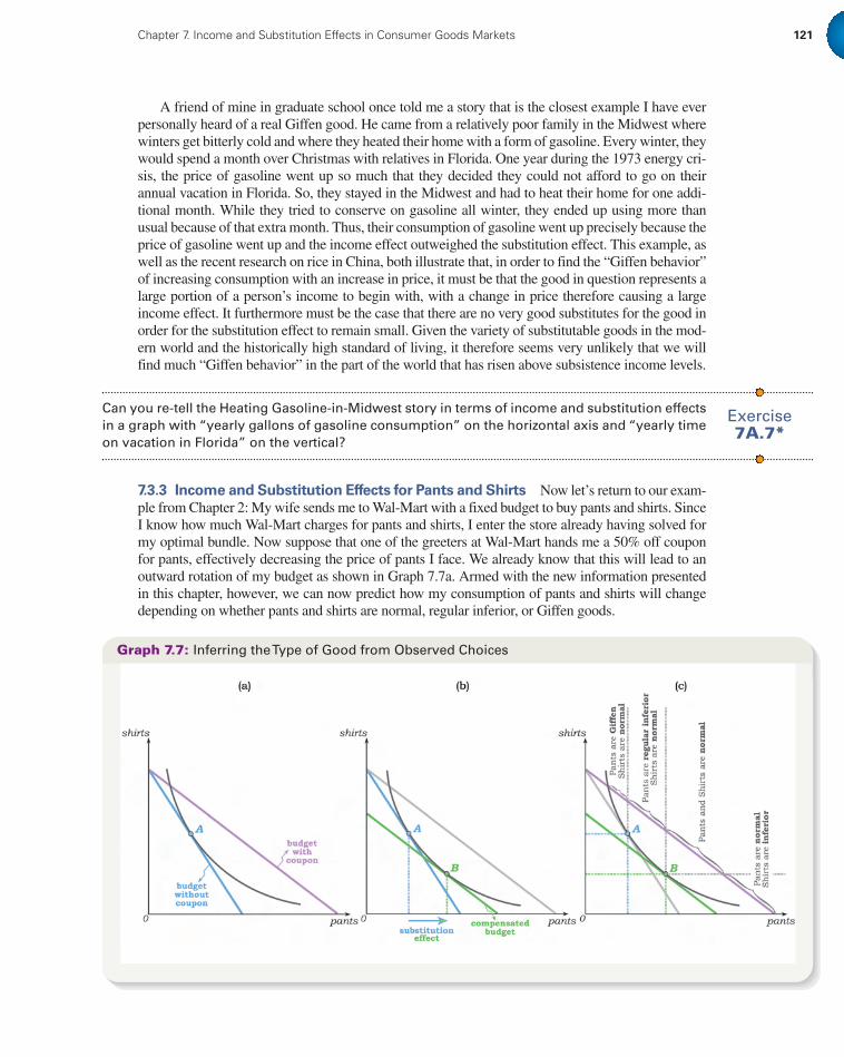
Graph 7.7: Inferring the Type of Good from Observed Choices

7.3.3 Income and Substitution Effects for Pants and Shirts Now let’s return to our exam-ple from Chapter 2: My wife sends me to Wal-Mart with a fixed budget to buy pants and shirts. SinceI know how much Wal-Mart charges for pants and shirts, I enter the store already having solved formy optimal bundle. Now suppose that one of the greeters at Wal-Mart hands me a 50% off couponfor pants, effectively decreasing the price of pants I face. We already know that this will lead to anoutward rotation of my budget as shown in Graph 7.7a. Armed with the new information presentedin this chapter, however, we can now predict how my consumption of pants and shirts will changedepending on whether pants and shirts are normal, regular inferior, or Giffen goods.

Can you re-tell the Heating Gasoline-in-Midwest story in terms of income and substitution effectsin a graph with “yearly gallons of gasoline consumption” on the horizontal axis and “yearly timeon vacation in Florida” on the vertical?

Exercise7A.7*

74707_07_ch07_p110-128.qxd 12/23/09 4:20 PM 1


First, we isolate once again the substitution effect by drawing my (green) compensatedbudget under the new price in Graph 7.7b. Notice that the “compensation” in this case is nega-tive: In order to keep my “real income” (i.e., my indifference curve) constant and concentrateonly on the impact of the change in opportunity costs, you would have to take away some of themoney my wife had given me. As always, the substitution effect, the shift from to , indicatesthat I will switch away from the good that has become relatively more expensive (shirts) andtoward the good that has become relatively cheaper (pants).

In Graph 7.7c, we then focus on what happens when we switch from the hypothetical opti-mum on the compensated (green) budget to our new optimum on the final (magenta) budget.Since this involves no change in opportunity costs, we are left with a pure income effect as wejump from the optimal point on the compensated budget line to the final optimum on the finalbudget constraint. Suppose we know that both shirts and pants are normal goods for me. Thiswould tell me that, when I experience an increase in income from the compensated to the finalbudget, I will choose to consume more pants and shirts than I did at point . If shirts are inferiorand pants are normal, I will consume more pants and fewer shirts than at ; and if pants are infe-rior and shirts are normal, I will consume fewer pants and more shirts. Given that I am restrictedin this example to consuming only shirts and pants, it cannot be the case that both goods are infe-rior because this would imply that I consume fewer pants and fewer shirts on my final budget thanI did at point , which would put me at a bundle to the southwest of . Since “more is better,” Iwould not be at an optimum given that I can move to a higher indifference curve from there.

Now suppose that you know not only that pants are an inferior good but also that pants are aGiffen good. The definition of a Giffen good implies that I will consume less of the good as itsprice decreases when exogenous income remains unchanged. Thus, I would end up consumingnot just fewer pants than at point but also fewer than at point . Notice that this is the onlyscenario under which we would not even have to first find the substitution effect; if we knowsomething is a Giffen good and we know its price has decreased, we immediately know that con-sumption will decrease as well. In each of the other scenarios, however, we needed to find thecompensated optimum before being able to apply the definition of normal or inferior goods.

Finally, suppose you know that shirts rather than pants are a Giffen good. Remember that inorder to observe a Giffen good, we must observe a price change for that good (with exogenousincome constant) since Giffen goods are goods whose consumption moves in the same directionas price (when income is exogenous and unchanged). In this example, we did not observe a pricechange for shirts, which means that we cannot usefully apply the definition of a Giffen good topredict how consumption will change. Rather, we can simply note that, since all Giffen goods arealso inferior goods, I will consume fewer shirts as my income increases from the compensatedbudget to the final budget. Thus, knowing that shirts are Giffen tells us nothing more in thisexample than knowing that shirts are inferior goods.

B

AB

BB

BB

B

BA

CONCLUSION

We have begun in this chapter to discuss the important concepts of income and substitution effects in thecontext of consumer goods markets. A more general theory of consumer behavior will emerge from thebuilding blocks of the optimization model we have laid, but we will not have completed the building of thistheory until Chapter 10. Before doing so, we will now first translate the concepts of income and substitutioneffects in consumer goods markets to similar ideas that emerge in labor and capital markets (Chapter 8). Wewill then illustrate in Chapters 9 and 10 how our notions of demand and consumer surplus relate directly toincome and substitution effects as introduced here.

Exercise7A.8

Replicate Graph 7.7 for an increase in the price of pants (rather than a decrease).

74707_07_ch07_p110-128.qxd 12/23/09 4:20 PM Page 122


There is no particular reason why it should be fully apparent to you at this point why these concepts areimportant. The importance will become clearer as we apply them in exercises and as we turn to some real-world issues later on. We did, however, raise one example in the introduction, and we can now make a bit moresense of it. We imagined a policy in which the government would reduce consumption of gasoline by taxing itheavily, only to turn around and distribute the revenues from the tax in the form of rebate checks. For many,including some very smart columnists and politicians, such a combination of a gasoline tax and rebate makesno sense; on average, they argue, consumers would receive back as much as they paid in gasoline taxes, and asa result, they would not change their behavior.11 Now that we have isolated income and substitution effects,however, we can see why economists think such a tax/rebate program will indeed curb gasoline consumption:The tax raises the price of gasoline and thus gives rise to income and substitution effects that (assuming gaso-line is a normal good) both result in less consumption of gasoline. The rebate, on the other hand, does notchange prices back; it simply causes incomes to rise above where they would otherwise have been after the tax.Thus, the rebate only causes an income effect in the opposite direction. The negative income effect from theincrease in the price should be roughly offset by the positive income effect from the tax rebate, which leavesus with a substitution effect that unambiguously implies a decrease in gasoline consumption.

END-OF-CHAPTER EXERCISES

7.1 Here, we consider some logical relationships between preferences and types of goods.

Suppose you consider all the goods that you might potentially want to consume.

a. Is it possible for all these goods to be luxury goods at every consumption bundle? Is it possiblefor all of them to be necessities?

b. Is it possible for all goods to be inferior goods at every consumption bundle? Is it possible forall of them to be normal goods?

c. True or False: When tastes are homothetic, all goods are normal goods.

d. True or False: When tastes are homothetic, some goods could be luxuries while others couldbe necessities.

e. True or False: When tastes are quasilinear, one of the goods is a necessity.

f. True or False: In a two-good model, if the two goods are perfect complements, they must bothbe normal goods.

g.* True or False: In a three-good model, if two of the goods are perfect complements, they mustboth be normal goods.

7.2 Suppose you have an income of $24 and the only two goods you consume are apples ( ) and peaches( ). The price of apples is $4 and the price of peaches is $3.

Suppose that your optimal consumption is 4 peaches and 3 apples.

a. Illustrate this in a graph using indifference curves and budget lines.

b. Now suppose that the price of apples falls to $2 and I take enough money away from you tomake you as happy as you were originally. Will you buy more or fewer peaches?

c. In reality, I do not actually take income away from you as described in (b), but your incomestays at $24 after the price of apples falls. I observe that, after the price of apples fell, you didnot change your consumption of peaches. Can you conclude whether peaches are an inferior ornormal good for you?

x2

x1

11This argument was in fact advanced by opponents of such a policy advocated by the Carter administration in the late 1970s,a proposal that won only 35 votes (out of 435) in the U.S. House of Representatives. It is not the only argument against suchpolicies. For instance, some have argued that a gasoline tax would be too narrow, and that the goals of such a tax would bebetter advanced by a broad-based carbon tax on all carbon-emmitting activity.*conceptually challenging†solutions in Study Guide

74707_07_ch07_p110-128.qxd 12/23/09 4:20 PM Page 123


7.3 Consider once again my tastes for Coke and Pepsi and my tastes for right and left shoes (as described inend-of-chapter exercise 6.2).

On two separate graphs—one with Coke and Pepsi on the axes, the other with right shoes and leftshoes—replicate your answers to end-of-chapter exercise 6.2(a) and (b). Label the original optimalbundles and the new optimal bundles .

a. In your Coke/Pepsi graph, decompose the change in consumer behavior into income andsubstitution effects by drawing the compensated budget and indicating the optimal bundle on that budget.

b. Repeat (a) for your right shoes/left shoes graph.

7.4 Return to the case of our beer and pizza consumption from end-of-chapter exercise 6.3.

Again, suppose you consume only beer and pizza (sold at prices and respectively) with anexogenously set income . Assume again some initial optimal (interior) bundle .

a. In 6.3(b), can you tell whether beer is normal or inferior? What about pizza?

b. When the price of beer goes up, I notice that you consume less beer. Can you tell whether beeris a normal or an inferior good?

c. When the price of beer goes down, I notice you buy less pizza. Can you tell whether pizza is anormal good?

d. When the price of pizza goes down, I notice you buy more beer. Is beer an inferior good foryou? Is pizza?

e. Which of your conclusions in part (d) would change if you knew pizza and beer are verysubstitutable?

7.5† Return to the analysis of my undying love for my wife expressed through weekly purchases of roses (asintroduced in end-of-chapter exercise 6.4).

Recall that initially roses cost $5 each and, with an income of $125 per week, I bought 25 roses eachweek. Then, when my income increased to $500 per week, I continued to buy 25 roses per week (atthe same price).

a. From what you observed thus far, are roses a normal or an inferior good for me? Are they aluxury or a necessity?

b. On a graph with weekly roses consumption on the horizontal and “other goods” on thevertical, illustrate my budget constraint when my weekly income is $125. Then illustrate thechange in the budget constraint when income remains $125 per week and the price of rosesfalls to $2.50. Suppose that my optimal consumption of roses after this price change rises to 50roses per week and illustrate this as bundle .

c. Illustrate the compensated budget line and use it to illustrate the income and substitutioneffects.

d. Now consider the case where my income is $500 and, when the price changes from $5 to$2.50, I end up consuming 100 roses per week (rather than 25). Assuming quasilinearity inroses, illustrate income and substitution effects.

e. True or False: Price changes of goods that are quasilinear give rise to no income effects for thequasilinear good unless corner solutions are involved.

7.6 Everyday Application: Housing Price Fluctuations: Part 2: Suppose, as in end-of-chapter exercise 6.9, youhave $400,000 to spend on “square feet of housing” and “all other goods.” Assume the same is true for me.

Suppose again that you initially face a $100 per square foot price for housing, and you choose to buya 2,000-square-foot house.

a. Illustrate this on a graph with square footage of housing on the horizontal axis and otherconsumption on the vertical. Then suppose, as you did in exercise 6.9, that the price of housingfalls to $50 per square foot after you bought your 2,000-square-foot house. Label the squarefootage of the house you would switch to .

b. Is smaller or larger than 2,000 square feet? Does your answer depend on whether housing isnormal, regular inferior, or Giffen?

hB

hB

C

AIp2p1

B

CA

EVERYDAYAPPL ICAT ION

74707_07_ch07_p110-128.qxd 12/23/09 4:20 PM Page 124


c. Now suppose that the price of housing had fallen to $50 per square foot before you boughtyour initial 2,000-square-foot house. Denote the size of house you would have bought andillustrate it in your graph.

d. Is larger than ? Is it larger than 2,000 square feet? Does your answer depend on whetherhousing is a normal, regular inferior, or Giffen good?

e. Now consider me. I did not buy a house until the price of housing was $50 per square foot, atwhich time I bought a 4,000-square-foot house. Then the price of housing rises to $100 persquare foot. Would I sell my house and buy a new one? If so, is the new house size largeror smaller than 4,000 square feet? Does your answer depend on whether housing is normal,regular inferior, or Giffen for me?

f. Am I better or worse off?

g. Suppose I had not purchased at the low price but rather purchased a house of size after theprice had risen to $100 per square foot. Is larger or smaller than ? Is it larger or smallerthan 4,000 square feet? Does your answer depend on whether housing is normal, regularinferior, or Giffen for me?

7.7 Everyday Application: Turkey and Thanksgiving: Every Thanksgiving, my wife and I debate abouthow we should prepare the turkey we will serve (and will then have left over). On the one hand, my wifelikes preparing turkeys the conventional way: roasted in the oven where it has to cook at 350 degrees for4 hours or so. I, on the other hand, like to fry turkeys in a big pot of peanut oil heated over a powerfulflame outdoors. The two methods have different costs and benefits. The conventional way of cookingturkeys has very little set-up cost (since the oven is already there and just has to be turned on) but arelatively large time cost from then on. (It takes hours to cook.) The frying method, on the other hand,takes some set-up (dragging out the turkey fryer, pouring gallons of peanut oil, etc., and then later thecleanup associated with it), but turkeys cook predictably quickly in just 3.5 minutes per pound.

As a household, we seem to be indifferent between doing it one way or another; sometimes we usethe oven, sometimes we use the fryer. But we have noticed that we cook much more turkey, severalturkeys, as a matter of fact, when we use the fryer than when we use the oven.

a. Construct a graph with “pounds of cooked turkeys” on the horizontal and “other consumption”on the vertical. (“Other consumption” here is not denominated in dollars as it normally is butrather in some consumption index that takes into account the time it takes to engage in suchconsumption.) Think of the set-up cost for frying turkeys and the waiting cost for cookingthem as the main costs that are relevant. Can you illustrate our family’s choice of whether tofry or roast turkeys at Thanksgiving as a choice between two “budget lines”?

b. Can you explain the fact that we seem to eat more turkey around Thanksgiving whenever wepull out the turkey fryer as opposed to roasting the turkey in the oven?

c. We have some friends who also struggle each Thanksgiving with the decision of whether to fry orroast, and they, too, seem to be indifferent between the two options. But we have noticed that theyonly cook a little more turkey when they fry than when they roast. What is different about them?

7.8*† Business Application: Sam’s Club and the Marginal Consumer: Superstores like Costco and Sam’sClub serve as wholesalers to businesses but also target consumers who are willing to pay a fixed fee inorder to get access to the lower wholesale prices offered in these stores. For purposes of this exercise,suppose that you can denote goods sold at superstores as and “dollars of other consumption” as .

Suppose all consumers have the same homothetic tastes over and , but they differ in theirincome. Every consumer is offered the same option of either shopping at stores with somewhat higherprices for or paying the fixed fee to shop at a superstore at somewhat lower prices for .

a. On a graph with on the horizontal axis and on the vertical, illustrate the regular budget(without a superstore membership) and the superstore budget for a consumer whose income issuch that these two budgets cross on the 45-degree line. Indicate on your graph a verticaldistance that is equal to the superstore membership fee .

b. Now consider a consumer with twice that much income. Where will this consumer’s twobudgets intersect relative to the 45-degree line?

c. Suppose consumer 1 (from part (a)) is just indifferent between buying and not buying thesuperstore membership. How will her behavior differ depending on whether or not she buysthe membership?

c

x2x1

x1cx1

x2x1

x2x1

hB œhC

œ

hCœ

hB

œ

hBhC

hC

EVERYDAYAPPL ICAT ION

BUS INESSAPPL ICAT ION

74707_07_ch07_p110-128.qxd 12/23/09 4:20 PM Page 125


d. If consumer 1 was indifferent between buying and not buying the superstore membership, canyou tell whether consumer 2 (from part (b)) is also indifferent? (Hint: Given that tastes arehomothetic and identical across consumers, what would have to be true about the intersectionof the two budgets for the higher income consumer in order for the consumer also to beindifferent between them?)

e. True or False: Assuming consumers have the same homothetic tastes, there exists a “mar-ginal” consumer with income such that all consumers with income greater than will buythe superstore membership and no consumer with income below will buy that membership.

f. True or False: By raising and/or , the superstore will lose relatively lower incomecustomers and keep high income customers.

g. Suppose you are a superstore manager and you think your store is overcrowded. You’d like toreduce the number of customers while at the same time increasing the amount each customerpurchases. How would you do this?

7.9* Business Application: Are Gucci Products Giffen Goods? We defined a Giffen good as a good thatconsumers (with exogenous incomes) buy more of when the price increases. When students first hear aboutsuch goods, they often think of luxury goods such as expensive Gucci purses and accessories. If themarketing departments for firms like Gucci are very successful, they may find a way of associating pricewith “prestige” in the minds of consumers, and this may allow them to raise the price and sell more products.But would that make Gucci products Giffen goods? The answer, as you will see in this exercise, is no.

Suppose we model a consumer who cares about the “practical value and style of Gucci products,”dollars of other consumption, and the “prestige value” of being seen with Gucci products. Denotethese as , , and respectively.

a. The consumer only has to buy and —the prestige value comes with the Gucciproducts. Let denote the price of Gucci products and be the price of dollars of otherconsumption. Illustrate the consumer’s budget constraint (assuming an exogenous income ).

b. The prestige value of Gucci purchases, , is something an individual consumer has nocontrol over. If is fixed at a particular level , the consumer therefore operates on atwo-dimensional slice of her three-dimensional indifference map over , , and . Drawsuch a slice for the indifference curve that contains the consumer’s optimal bundle on thebudget from part (a).

c. Now suppose that Gucci manages to raise the prestige value of its products and thus thatcomes with the purchase of Gucci products. For now, suppose they do this without changing

. This implies you will shift to a different two-dimensional slice of your three-dimensionalindifference map. Illustrate the new two-dimensional indifference curve that contains . Is thenew at greater or smaller in absolute value than it was before?

d.* Would the consumer consume more or fewer Gucci products after the increase in prestige value?

e. Now suppose that Gucci manages to convince consumers that Gucci products become moredesirable the more expensive they are. Put differently, the prestige value is linked to , theprice of the Gucci products. On a new graph, illustrate the change in the consumer’s budget asa result of an increase in .

f. Suppose that our consumer increases her purchases of Gucci products as a result of the increasein the price . Illustrate two indifference curves: one that gives rise to the original optimum and another that gives rise to the new optimum . Can these indifference curves cross?

g. Explain why, even though the behavior is consistent with what we would expect if Gucciproducts were a Giffen good, Gucci products are not a Giffen good in this case.

h. In a footnote in the chapter, we defined the following: A good is a Veblen good if preferencesfor the good change as price increases, with this change in preferences possibly leading to anincrease in consumption as price increases. Are Gucci products a Veblen good in this exercise?

7.10 Policy Application: Tax Deductibility and Tax Credits: In end-of-chapter exercise 2.17, you wereasked to think about the impact of tax deductibility on a household’s budget constraint.

Suppose we begin in a system in which mortgage interest is not deductible and then tax deductibilityof mortgage interest is introduced.

CAp1

p1

p1x3

AMRSA

p1

x3

Ax3x2x1

x3x3

x3

Ip2 = 1p1

x3x2x1

x3x2x1

p1c

III

BUS INESSAPPL ICAT ION

POL ICYAPPL ICAT ION

74707_07_ch07_p110-128.qxd 12/23/09 4:20 PM Page 126


a. Using a graph (as you did in exercise 2.17) with “square feet of housing” on the horizontalaxis and “dollars of other consumption” on the vertical, illustrate the direction of the substitu-tion effect.

b. What kind of good would housing have to be in order for the household to consume lesshousing as a result of the introduction of the tax deductibility program?

c. On a graph that contains both the before and after deductibility budget constraints, how wouldyou illustrate the amount of subsidy the government provides to this household?

d. Suppose the government provided the same amount of money to this household but did soinstead by simply giving it to the household as cash back on its taxes (without linking it tohousing consumption). Will the household buy more or less housing?

e. Will the household be better or worse off?

f. Do your answers to (d) and (e) depend on whether housing is normal, regular inferior, orGiffen?

g. Under tax deductibility, will the household spend more on other consumption before or aftertax deductibility is introduced? Discuss your answer in terms of income and substitutioneffects and assume that “other goods” is a normal good.

h. If you observed that a household consumes more in “other goods” after the introduction of taxdeductibility, could that household’s tastes be quasilinear in housing? Could they be homothetic?

7.11 Policy Application: Substitution Effects and Social Security Cost of Living Adjustments: In end-of-chapter exercise 6.16, you investigated the government’s practice for adjusting Social Security incomefor seniors by ensuring that the average senior can always afford to buy some average bundle of goodsthat remains fixed. To simplify the analysis, let us again assume that the average senior consumes onlytwo different goods.

Suppose that last year our average senior optimized at the average bundle identified by thegovernment, and begin by assuming that we denominate the units of and such that last year

.

a. Suppose that increases. On a graph with on the horizontal and on the vertical axis,illustrate the compensated budget and the bundle that, given your senior’s tastes, would keepthe senior just as well off at the new price.

b. In your graph, compare the level of income the senior requires to get to bundle with theincome required to get him back to bundle .

c. What determines the size of the difference in the income necessary to keep the senior just aswell off when the price of good 1 increases as opposed to the income necessary for the seniorstill to be able to afford bundle ?

d. Under what condition will the two forms of compensation be identical?

e. You should recognize the move from to as a pure substitution effect as we have defined itin this chapter. Often this substitution effect is referred to as the Hicksian substitution effect,defined as the change in behavior when opportunity costs change but the consumer receivessufficient compensation to remain just as happy. Let be the consumption bundle theaverage senior would choose when compensated so as to be able to afford the original bundle

. The movement from to is often called the Slutsky substitution effect, defined as thechange in behavior when opportunity costs change but the consumer receives sufficientcompensation to be able to afford to stay at the original consumption bundle. True or False:The government could save money by using Hicksian rather than Slutsky substitutionprinciples to determine appropriate cost of living adjustments for Social Security recipients.

f. True or False: Hicksian and Slutsky compensation get closer to one another the smaller theprice changes.

7.12*† Policy Application: Fuel Efficiency, Gasoline Consumption, and Gas Prices: Policy makers frequentlysearch for ways to reduce consumption of gasoline. One straightforward option is to tax gasoline,thereby encouraging consumers to drive less and switch to more fuel-efficient cars.

Suppose that you have tastes for driving and for other consumption, and assume throughout that yourtastes are homothetic.

B¿AA

B¿

BA

A

AB

Bx2x1p1

p1 = p2 = 1x2x1

A



74707_07_ch07_p110-128.qxd 12/23/09 4:20 PM Page 127


a. On a graph with monthly miles driven on the horizontal and “monthly other consumption” onthe vertical axis, illustrate two budget lines: one in which you own a gas-guzzling car, whichhas a low monthly payment (that has to be made regardless of how much the car is driven) buthigh gasoline use per mile; the other in which you own a fuel-efficient car, which has a highmonthly payment that has to be made regardless of how much the car is driven but uses lessgasoline per mile. Draw this in such a way that it is possible for you to be indifferent betweenowning the gas-guzzling and the fuel-efficient car.

b. Suppose you are indeed indifferent. With which car will you drive more?

c. Can you tell with which car you will use more gasoline? What does your answer depend on?

d. Now suppose that the government imposes a tax on gasoline, and this doubles the opportunitycost of driving both types of cars. If you were indifferent before the tax was imposed, can younow say whether you will definitively buy one car or the other (assuming you waited to buy acar until after the tax is imposed)? What does your answer depend on? (Hint: It may be helpfulto consider the extreme cases of perfect substitutes and perfect complements before derivingyour general conclusion to this question.)

e. The empirical evidence suggests that consumers shift toward more fuel-efficient cars when theprice of gasoline increases. True or False: This would tend to suggest that driving and othergood consumption are relatively complementary.

f. Suppose an increase in gasoline taxes raises the opportunity cost of driving a mile with a fuel-efficient car to the opportunity cost of driving a gas guzzler before the tax increase. Willsomeone who was previously indifferent between a fuel-efficient and a gas-guzzling car nowdrive more or less in a fuel-efficient car than he did in a gas guzzler prior to the tax increase?(Continue with the assumption that tastes are homothetic.)

7.13 Policy Application: Public Housing and Housing Subsidies: In exercise 2.14, you considered twodifferent public housing programs in parts (a) and (b), one where a family is simply offered a particularapartment for a below-market rent and another where the government provides a housing price subsidythat the family can use anywhere in the private rental market.

Suppose we consider a family that earns $1,500 per month and either pays $0.50 per square foot inmonthly rent for an apartment in the private market or accepts a 1,500-square-foot government publichousing unit at the government’s price of $500 per month.

a. On a graph with square feet of housing and “dollars of other consumption,” illustrate two caseswhere the family accepts the public housing unit, one where this leads them to consume lesshousing than they otherwise would and another where it leads them to consume more housingthan they otherwise would.

b. If we use the members of the household’s own judgment about the household’s well-being, is italways the case that the option of public housing makes the participating households better off?

c. If the policy goal behind public housing is to increase the housing consumption of the poor, isit more or less likely to succeed the less substitutable housing and other goods are?

d. What is the government’s opportunity cost of owning a public housing unit of 1,500 squarefeet? How much does it therefore cost the government to provide the public housing unit tothis family?

e. Now consider instead a housing price subsidy under which the government tells qualifiedfamilies that it will pay some fraction of their rental bills in the private housing market. If thisrental subsidy is set so as to make the household just as well off as it was under publichousing, will it lead to more or less consumption of housing than if the household choosespublic housing?

f. Will giving such a rental subsidy cost more or less than providing the public housing unit?What does your answer depend on?

g. Suppose instead that the government simply gave cash to the household. If it gave sufficientcash to make the household as well off as it is under the public housing program, would it cost the government more or less than $250? Can you tell whether under such a subsidy thehousehold consumes more or less housing than under public housing?


74707_07_ch07_p110-128.qxd 12/23/09 4:20 PM Page 128

Income and Substitution Effects in Consumer Goods Markets · 1Chapters 2 and 4 through 6 are...

Documents

Transcript of Income and Substitution Effects in Consumer Goods Markets · 1Chapters 2 and 4 through 6 are...