Income and Poverty in the United States: 2014 - …and+poverty+in+the+US.pdfU.S. Census Bureau...

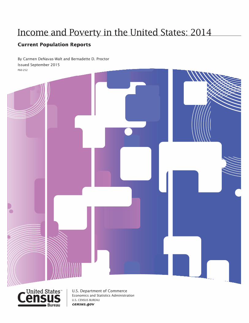
Income and Poverty in the United States: 2014Current Population Reports

Issued September 2015P60-252

By Carmen DeNavas-Walt and Bernadette D. Proctor

U.S. Census Bureau Income and Poverty in the United States: 2014 5

INCOME IN THE UNITED STATES

Highlights

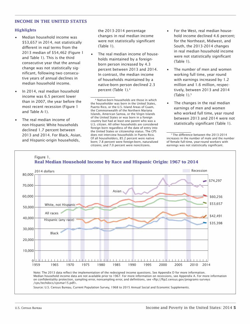
• Median household income was $53,657 in 2014, not statistically different in real terms from the 2013 median of $54,462 (Figure 1 and Table 1). This is the third consecutive year that the annual change was not statistically sig-nificant, following two consecu-tive years of annual declines in median household income.

• In 2014, real median household income was 6.5 percent lower than in 2007, the year before the most recent recession (Figure 1 and Table A-1).

• The real median income of non-Hispanic White households declined 1.7 percent between 2013 and 2014. For Black, Asian, and Hispanic-origin households,

the 2013-2014 percentage changes in real median income were not statistically significant (Table 1).

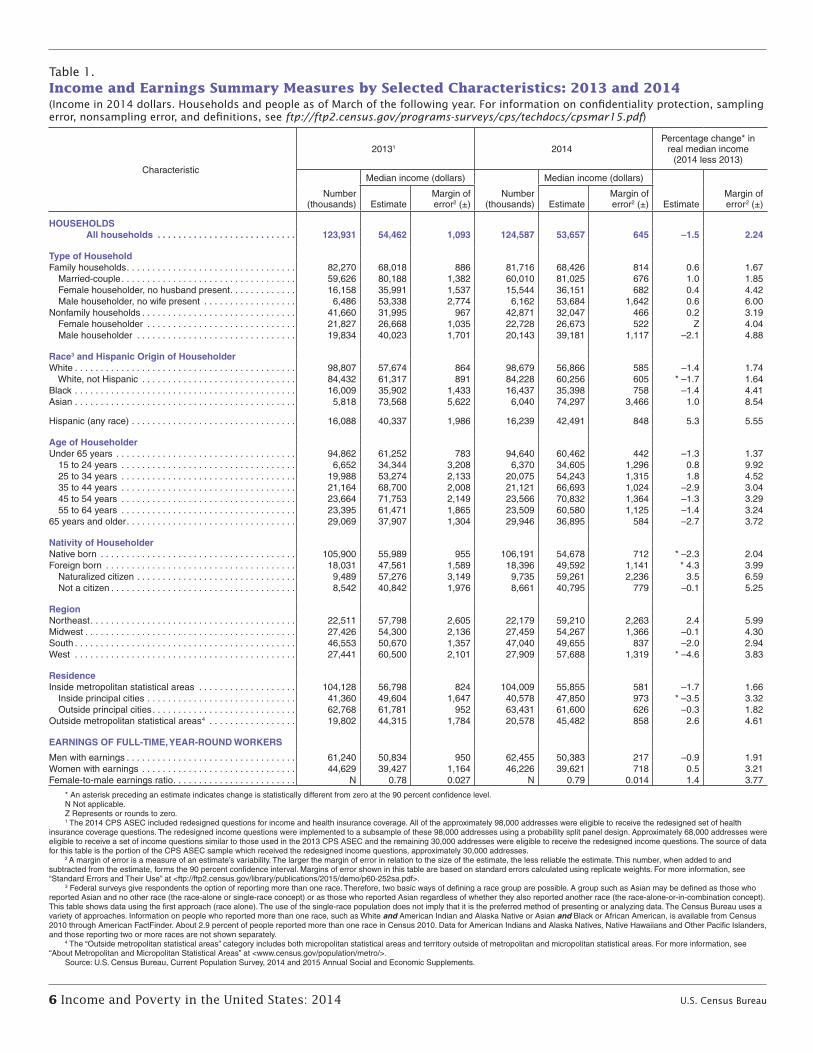
• The real median income of house-holds maintained by a foreign-born person increased by 4.3 percent between 2013 and 2014. In contrast, the median income of households maintained by a native-born person declined 2.3 percent (Table 1).4

4 Native-born households are those in which the householder was born in the United States, Puerto Rico, or the U.S. Island Areas of Guam, the Commonwealth of the Northern Mariana Islands, American Samoa, or the Virgin Islands of the United States or was born in a foreign country but had at least one parent who was a U.S. citizen. All other households are considered foreign born regardless of the date of entry into the United States or citizenship status. The CPS does not interview households in Puerto Rico. Of all householders, 85.2 percent were native born; 7.8 percent were foreign-born, naturalized citizens; and 7.0 percent were noncitizens.

• For the West, real median house-hold income declined 4.6 percent; for the Northeast, Midwest, and South, the 2013-2014 changes in real median household income were not statistically significant (Table 1).

• The number of men and women working full time, year round with earnings increased by 1.2 million and 1.6 million, respec-tively, between 2013 and 2014 (Table 1).5

• The changes in the real median earnings of men and women who worked full time, year round between 2013 and 2014 were not statistically significant (Table 1).

5 The difference between the 2013-2014 increases in the number of male and the number of female full-time, year-round workers with earnings was not statistically significant.

Figure 1.Real Median Household Income by Race and Hispanic Origin: 1967 to 2014

Note: The 2013 data reflect the implementation of the redesigned income questions. See Appendix D for more information. Median household income data are not available prior to 1967. For more information on recessions, see Appendix A. For more information on confidentiality protection, sampling error, nonsampling error, and definitions, see <ftp://ftp2.census.gov/programs-surveys/cps/techdocs/cpsmar15.pdf>.

Source: U.S. Census Bureau, Current Population Survey, 1968 to 2015 Annual Social and Economic Supplements.

2014 dollars Recession

0

10,000

20,000

30,000

40,000

50,000

60,000

70,000

80,000

2014201020052000 19951990198519801975197019651959

$74,297

$60,256

$53,657

$42,491

$35,398

All races

White, not Hispanic

Black

Asian

Hispanic (any race)

6 Income and Poverty in the United States: 2014 U.S. Census Bureau

Table 1.Income and Earnings Summary Measures by Selected Characteristics: 2013 and 2014(Income in 2014 dollars. Households and people as of March of the following year. For information on confidentiality protection, sampling error, nonsampling error, and definitions, see ftp://ftp2.census.gov/programs-surveys/cps/techdocs/cpsmar15.pdf)

Characteristic

20131 2014Percentage change* in

real median income (2014 less 2013)

Number (thousands)

Median income (dollars)

Number (thousands)

Median income (dollars)

EstimateMargin of error 2 (±)Estimate

Margin of error2 (±) Estimate

Margin of error2 (±)

HOUSEHOLDS All households . . . . . . . . . . . . . . . . . . . . . . . . . . . 123,931 54,462 1,093 124,587 53,657 645 –1.5 2.24

Type of HouseholdFamily households . . . . . . . . . . . . . . . . . . . . . . . . . . . . . . . . . 82,270 68,018 886 81,716 68,426 814 0.6 1.67 Married-couple . . . . . . . . . . . . . . . . . . . . . . . . . . . . . . . . . . 59,626 80,188 1,382 60,010 81,025 676 1.0 1.85 Female householder, no husband present . . . . . . . . . . . . . 16,158 35,991 1,537 15,544 36,151 682 0.4 4.42 Male householder, no wife present . . . . . . . . . . . . . . . . . . 6,486 53,338 2,774 6,162 53,684 1,642 0.6 6.00Nonfamily households . . . . . . . . . . . . . . . . . . . . . . . . . . . . . . 41,660 31,995 967 42,871 32,047 466 0.2 3.19 Female householder . . . . . . . . . . . . . . . . . . . . . . . . . . . . . 21,827 26,668 1,035 22,728 26,673 522 Z 4.04 Male householder . . . . . . . . . . . . . . . . . . . . . . . . . . . . . . . 19,834 40,023 1,701 20,143 39,181 1,117 –2.1 4.88

Race3 and Hispanic Origin of HouseholderWhite . . . . . . . . . . . . . . . . . . . . . . . . . . . . . . . . . . . . . . . . . . . 98,807 57,674 864 98,679 56,866 585 –1.4 1.74 White, not Hispanic . . . . . . . . . . . . . . . . . . . . . . . . . . . . . . 84,432 61,317 891 84,228 60,256 605 * –1.7 1.64Black . . . . . . . . . . . . . . . . . . . . . . . . . . . . . . . . . . . . . . . . . . . 16,009 35,902 1,433 16,437 35,398 758 –1.4 4.41Asian . . . . . . . . . . . . . . . . . . . . . . . . . . . . . . . . . . . . . . . . . . . 5,818 73,568 5,622 6,040 74,297 3,466 1.0 8.54

Hispanic (any race) . . . . . . . . . . . . . . . . . . . . . . . . . . . . . . . . 16,088 40,337 1,986 16,239 42,491 848 5.3 5.55

Age of HouseholderUnder 65 years . . . . . . . . . . . . . . . . . . . . . . . . . . . . . . . . . . . 94,862 61,252 783 94,640 60,462 442 –1.3 1.37 15 to 24 years . . . . . . . . . . . . . . . . . . . . . . . . . . . . . . . . . . 6,652 34,344 3,208 6,370 34,605 1,296 0.8 9.92 25 to 34 years . . . . . . . . . . . . . . . . . . . . . . . . . . . . . . . . . . 19,988 53,274 2,133 20,075 54,243 1,315 1.8 4.52 35 to 44 years . . . . . . . . . . . . . . . . . . . . . . . . . . . . . . . . . . 21,164 68,700 2,008 21,121 66,693 1,024 –2.9 3.04 45 to 54 years . . . . . . . . . . . . . . . . . . . . . . . . . . . . . . . . . . 23,664 71,753 2,149 23,566 70,832 1,364 –1.3 3.29 55 to 64 years . . . . . . . . . . . . . . . . . . . . . . . . . . . . . . . . . . 23,395 61,471 1,865 23,509 60,580 1,125 –1.4 3.2465 years and older . . . . . . . . . . . . . . . . . . . . . . . . . . . . . . . . . 29,069 37,907 1,304 29,946 36,895 584 –2.7 3.72

Nativity of HouseholderNative born . . . . . . . . . . . . . . . . . . . . . . . . . . . . . . . . . . . . . . 105,900 55,989 955 106,191 54,678 712 * –2.3 2.04Foreign born . . . . . . . . . . . . . . . . . . . . . . . . . . . . . . . . . . . . . 18,031 47,561 1,589 18,396 49,592 1,141 * 4.3 3.99 Naturalized citizen . . . . . . . . . . . . . . . . . . . . . . . . . . . . . . . 9,489 57,276 3,149 9,735 59,261 2,236 3.5 6.59 Not a citizen . . . . . . . . . . . . . . . . . . . . . . . . . . . . . . . . . . . . 8,542 40,842 1,976 8,661 40,795 779 –0.1 5.25

RegionNortheast . . . . . . . . . . . . . . . . . . . . . . . . . . . . . . . . . . . . . . . . 22,511 57,798 2,605 22,179 59,210 2,263 2.4 5.99Midwest . . . . . . . . . . . . . . . . . . . . . . . . . . . . . . . . . . . . . . . . . 27,426 54,300 2,136 27,459 54,267 1,366 –0.1 4.30South . . . . . . . . . . . . . . . . . . . . . . . . . . . . . . . . . . . . . . . . . . . 46,553 50,670 1,357 47,040 49,655 837 –2.0 2.94West . . . . . . . . . . . . . . . . . . . . . . . . . . . . . . . . . . . . . . . . . . . 27,441 60,500 2,101 27,909 57,688 1,319 * –4.6 3.83

ResidenceInside metropolitan statistical areas . . . . . . . . . . . . . . . . . . . 104,128 56,798 824 104,009 55,855 581 –1.7 1.66 Inside principal cities . . . . . . . . . . . . . . . . . . . . . . . . . . . . . 41,360 49,604 1,647 40,578 47,850 973 * –3.5 3.32 Outside principal cities . . . . . . . . . . . . . . . . . . . . . . . . . . . . 62,768 61,781 952 63,431 61,600 626 –0.3 1.82Outside metropolitan statistical areas 4 . . . . . . . . . . . . . . . . . 19,802 44,315 1,784 20,578 45,482 858 2.6 4.61

EARNINGS OF FULL-TIME, YEAR-ROUND WORKERS

Men with earnings . . . . . . . . . . . . . . . . . . . . . . . . . . . . . . . . . 61,240 50,834 950 62,455 50,383 217 –0.9 1.91Women with earnings . . . . . . . . . . . . . . . . . . . . . . . . . . . . . . 44,629 39,427 1,164 46,226 39,621 718 0.5 3.21Female-to-male earnings ratio . . . . . . . . . . . . . . . . . . . . . . . . N 0.78 0.027 N 0.79 0.014 1.4 3.77

* An asterisk preceding an estimate indicates change is statistically different from zero at the 90 percent confidence level. N Not applicable.Z Represents or rounds to zero.1 The 2014 CPS ASEC included redesigned questions for income and health insurance coverage. All of the approximately 98,000 addresses were eligible to receive the redesigned set of health

insurance coverage questions. The redesigned income questions were implemented to a subsample of these 98,000 addresses using a probability split panel design. Approximately 68,000 addresses were eligible to receive a set of income questions similar to those used in the 2013 CPS ASEC and the remaining 30,000 addresses were eligible to receive the redesigned income questions. The source of data for this table is the portion of the CPS ASEC sample which received the redesigned income questions, approximately 30,000 addresses.

2 A margin of error is a measure of an estimate’s variability. The larger the margin of error in relation to the size of the estimate, the less reliable the estimate. This number, when added to and subtracted from the estimate, forms the 90 percent confidence interval. Margins of error shown in this table are based on standard errors calculated using replicate weights. For more information, see “Standard Errors and Their Use” at <ftp://ftp2.census.gov/library/publications/2015/demo/p60-252sa.pdf>.

3 Federal surveys give respondents the option of reporting more than one race. Therefore, two basic ways of defining a race group are possible. A group such as Asian may be defined as those who reported Asian and no other race (the race-alone or single-race concept) or as those who reported Asian regardless of whether they also reported another race (the race-alone-or-in-combination concept). This table shows data using the first approach (race alone). The use of the single-race population does not imply that it is the preferred method of presenting or analyzing data. The Census Bureau uses a variety of approaches. Information on people who reported more than one race, such as White and American Indian and Alaska Native or Asian and Black or African American, is available from Census 2010 through American FactFinder. About 2.9 percent of people reported more than one race in Census 2010. Data for American Indians and Alaska Natives, Native Hawaiians and Other Pacific Islanders, and those reporting two or more races are not shown separately.

4 The “Outside metropolitan statistical areas” category includes both micropolitan statistical areas and territory outside of metropolitan and micropolitan statistical areas. For more information, see “About Metropolitan and Micropolitan Statistical Areas” at <www.census.gov/population/metro/>.

Source: U.S. Census Bureau, Current Population Survey, 2014 and 2015 Annual Social and Economic Supplements.


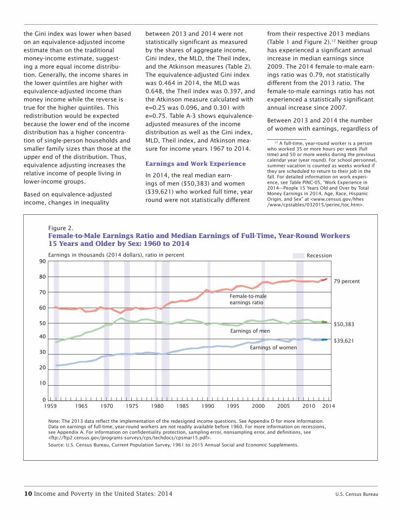
• The 2014 female-to-male earn-ings ratio was 0.79, not statisti-cally different from the 2013 ratio (Table 1 and Figure 2).

• There were more women full-time, year-round workers with earnings in 2014 than in 2007, the year before the most recent recession (Table A-4). For male full-time, year-round workers with earnings, the difference between the 2014 and 2007 estimates was not statistically significant.

• The real median earnings of full-time, year-round working women in 2014 were not statistically dif-ferent from their median in 2007, the year before the most recent recession. The median earnings of full-time, year-round working men were 2.2 percent lower in 2014 than in 2007 (Table A-4).

Household Income

Median household income was $53,657 in 2014, not statistically different from the 2013 median in real terms, 6.5 percent lower than the 2007 (the year before the most recent recession) median ($57,357), and 7.2 percent lower than the median household income peak ($57,843) that occurred in 1999 (Figure 1 and Table A-1).6

Type of Household

Real median incomes in 2014 of family households, $68,426, and nonfamily households, $32,047, were not statistically different from their respective 2013 medians (Table 1). For the specific types of family and nonfamily households, changes in real income between 2013 and 2014 were also not statistically signifi-cant. Family households have not

6 The difference between the 1999 and 2007 median household incomes was not statistically significant. The difference between the 2007-2014 and 1999-2014 percentage changes (6.5 and 7.2 percent, respectively) was not statisti-cally significant.

experienced an annual increase in median household income since 2007. The last increase for nonfamily households was in 2009.

For family households, married-couple households had the highest median income in 2014 ($81,025), followed by households maintained by men with no wife present ($53,684). Those maintained by women with no hus-band present had the lowest median ($36,151).

Race and Hispanic Origin

The real median income of non-Hispanic White households declined by 1.7 percent between 2013 and 2014, from $61,317 to $60,256. For Black, Asian, and Hispanic-origin households, the 2013-2014 percent-age changes in real median household income were not statistically signifi-cant (Table 1). Non-Hispanic White and Black households last experienced an annual increase in median income in 2007, and Asian household’s last annual increase was in 1999. Hispanic households experienced an annual increase in 2013.

Among the race groups, Asian households had the highest median income in 2014 ($74,297). The median income of non-Hispanic White households was $60,256, and for Black households it was $35,398 (Table 1 and Figure 1). For Hispanic households, the median income was $42,491.

The real median income of Asian households in 2014 was not statisti-cally different from the pre-2001- recession peak.7 Whereas, household income in 2014 was 4.0 percent lower for non-Hispanic Whites (from $62,762 in 1999), 13.2 percent lower for Blacks (from $40,783 in 2000),

7 The difference between the real median income of Asian households in 2014 and 2000 was not statistically significant.

and 6.8 percent lower for Hispanics (from $45,596 in 2000) (Table A-1).8

Comparing the 2014 income of non-Hispanic White households with that of other households shows that the ratio of Asian to non-Hispanic White income was 1.23, the ratio of Black to non-Hispanic White income was 0.59, and the ratio of Hispanic to non-Hispanic White income was 0.71. Between 1972 and 2014, the change in the Black to non-Hispanic White income ratio was not statistically significant.9 Over the same period, the Hispanic to non-Hispanic White income ratio declined from 0.74 to 0.71. Income data for the Asian population was first available in 1987. The 2014 Asian to non-Hispanic White income ratio was not statistically dif-ferent from the 1987 ratio.

Age of Householder

Between 2013 and 2014, there were no statistically significant changes in household income by age of the householders. Households main-tained by householders aged 45 to 54 had the highest median income in 2014 ($70,832), followed by those with householders aged 35 to 44 ($66,693), those with householders aged 55 to 64 ($60,580), household-ers aged 25 to 34 ($54,243), and those with householders aged 65 and older ($36,895). Households main-tained by householders aged 15 to 24 had the lowest median income ($34,605).

8 The difference between the declines for non-Hispanic White households and Hispanic households was not statistically significant. For non-Hispanic White households, the $62,762 income peak in 1999 was not statistically dif-ferent from their 2000 median of $62,718. For Blacks, the $40,783 income peak in 2000 was not statistically different from their 1999 median of $39,669. For Hispanics, the $45,596 income peak in 2000 was not statistically different from their 2001 median of $44,882.

9 The first year that income data for the Hispanic and non-Hispanic White populations were collected in the CPS ASEC was 1972.


Nativity

Change in real median household income between 2013 and 2014 var-ied by nativity of the householder. The income of households maintained by a foreign-born person increased 4.3 percent, from $47,561 to $49,592; while the median income of house-holds maintained by a native-born person declined 2.3 percent, from $55,989 to $54,678. The median incomes of households maintained by a naturalized citizen ($59,261) or a noncitizen ($40,795), in 2014, were not statistically different from their respective 2013 medians (Table 1).

In 2014, households maintained by a naturalized citizen ($59,261) had the highest median household income, followed by households maintained by a native-born person ($54,678). Households maintained by a nonciti-zen had the lowest household income ($40,795) (Table 1).

Region10

Households in the West experi-enced a 4.6 percent decline in real median income between 2013 and 2014, whereas the apparent changes in income of households in the Northeast, Midwest, and South were not statistically significant. Households with the highest median household incomes were in the Northeast ($59,210) and the West

10 The Northeast region includes Connecticut, Maine, Massachusetts, New Hampshire, New Jersey, New York, Pennsylvania, Rhode Island, and Vermont. The Midwest region includes Illinois, Indiana, Iowa, Kansas, Michigan, Minnesota, Missouri, Nebraska, North Dakota, Ohio, South Dakota, and Wisconsin. The South region includes Alabama, Arkansas, Delaware, Florida, Georgia, Kentucky, Louisiana, Maryland, Mississippi, North Carolina, Oklahoma, South Carolina, Tennessee, Texas, Virginia, West Virginia, and the District of Columbia, a state equivalent. The West region includes Alaska, Arizona, California, Colorado, Hawaii, Idaho, Montana, Nevada, New Mexico, Oregon, Utah, Washington, and Wyoming.

($57,688), followed by the Midwest ($54,267) and the South ($49,655) (Table 1).11

Residence

In 2014, households within metro-politan areas but outside principal cities had the highest median income ($61,600), while households outside metropolitan areas had the lowest ($45,482). Between 2013 and 2014, the real income of households inside principal cities declined 3.5 percent, while the changes in median incomes of households for the remaining three residential categories shown in Table 1 were not statistically significant.

Income Inequality

The Census Bureau traditionally reports two measures of income inequality: (1) the shares of aggregate household income received by quin-tiles and (2) the Gini index. In addition to these measures, the Census Bureau also produces estimates of the ratio of income percentiles; the Theil index, which is similar to the Gini index in that it is a single statistic that summa-rizes the dispersion of income across the entire income distribution; the mean logarithmic deviation of income (MLD), which measures the gap between median and average income; and the Atkinson measure, which is useful in determining which end of the income distribution contributed most to inequality.12

Changes in income inequality between 2013 and 2014 were not statistically significant as measured by the shares of aggregate household income by quintiles, the Gini index,

11 The difference between the median house-hold incomes for the Northeast and the West was not statistically significant.

12 An article by Paul Allison, “Measures of Inequality,” American Sociological Review, 43, December 1977, pp. 865–880, provides an explanation of inequality measures.

the MLD, the Theil index, and the Atkinson measures (Table 2 and A-2). Households in the lowest quintile had incomes of $21,432 or less in 2014. Households in the second quintile had incomes between $21,433 and $41,186, those in the third quintile had incomes between $41,187 and $68,212, and those in the fourth quin-tile had incomes between $68,213 and $112,262. Households in the highest quintile had incomes of $112,263 or more. The top 5 percent had incomes of $206,568 or more.

The Gini index was 0.480 in 2014, not statistically different from 2013. Since 1993, the earliest year available for comparable measures of income inequality, the Gini index was up 5.9 percent (Table A-2).13, 14, 15

Comparing changes in household income at selected percentiles shows that income inequality has increased between 1999 (the year that house-hold income peaked before the 2001 recession) and 2014 (Table A-2). Incomes at the 50th and 10th percen-tiles declined 7.2 percent and 16.5 percent, respectively, while income at the 90th percentile increased 2.8 percent between 1999 and 2014. In 2014, the 90th to 10th percen-tile income ratio was 12.83, not statistically different from the 2013 ratio. Since 1999, the 90th to 10th

13 Exercise caution when making direct com-parisons with years earlier than 1993 because of substantial methodological changes in the 1994 CPS ASEC. In that year, the Census Bureau introduced computer-assisted interviewing and increased income reporting limits.

14 For further discussion of how high incomes reported in the CPS ASEC affect income distri-bution measures, see Jessica Semega and Ed Welniak, “Evaluating the Impact of Unrestricted Income Values on Income Distribution Measures Using the Current Population Survey’s Annual Social and Economic Supplement (ASEC),” April 2007, <www.census.gov/hhes/www/income /publications/unrestrict-tables/index.html>.

15 The calculated percentage change is differ-ent due to rounded components.


percentile income ratio increased 23.1 percent.

Equivalence-Adjusted Income Inequality

Another way to measure income inequality is to use an equivalence-adjusted income estimate that takes into consideration the number of people living in the household and how these people share resources and take advantage of economies of scale. For example, the money-income-based distribution treats an income of $30,000 for a single-person house-hold and a family household similarly,

while the equivalence-adjusted income of $30,000 for a single-person household would be more than twice the equivalence-adjusted income of $30,000 for a family household with two adults and two children. The equivalence adjustment used here is based on a three-parameter scale16 that reflects:

16 The three-parameter scale used here is the same as the one used in the Supplemental Poverty Measure. For details on the deriva-tion of the three-parameter scale, see Kathleen Short, The Supplemental Poverty Measure: 2013, Current Population Reports, P60-251, U.S. Census Bureau, October 2014, <www.census.gov /content/dam/Census/library/publications /2014/demo/p60-251.pdf>.

1. On average, children consume less than adults.

2. As family size increases, expenses do not increase at the same rate.

3. The increase in expenses is larger for a first child of a single-parent family than the first child of a two-adult family.

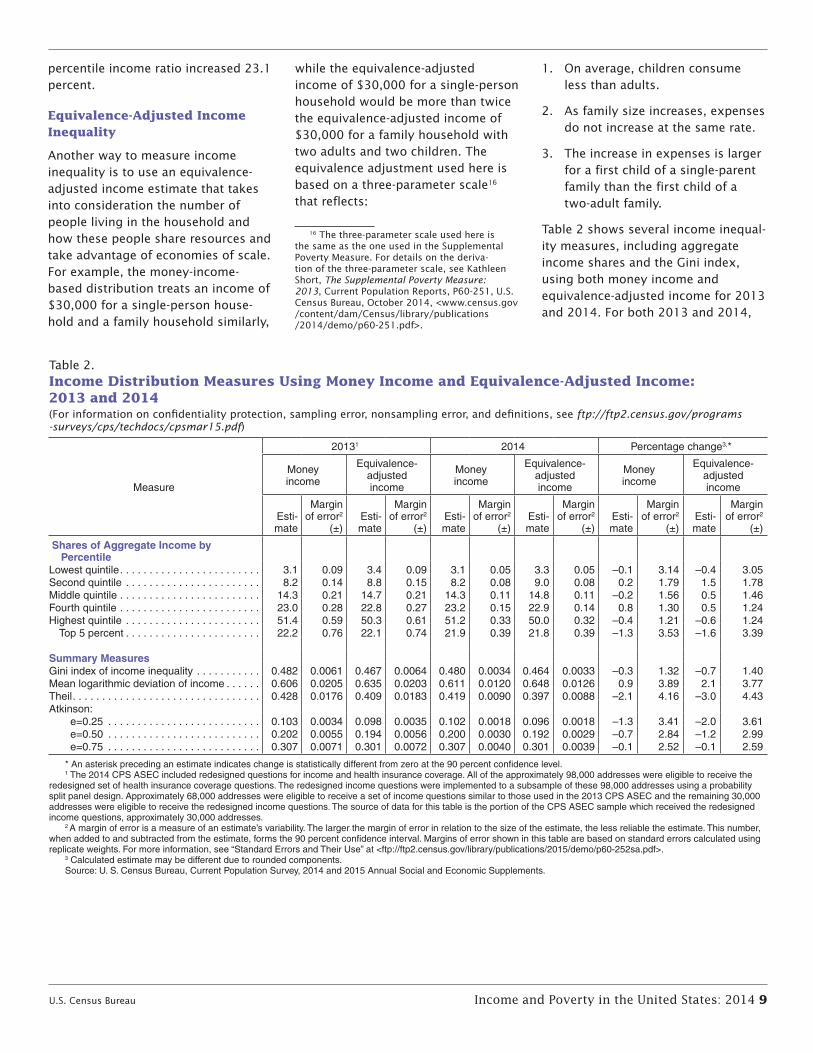
Table 2 shows several income inequal-ity measures, including aggregate income shares and the Gini index, using both money income and equivalence-adjusted income for 2013 and 2014. For both 2013 and 2014,

Table 2. Income Distribution Measures Using Money Income and Equivalence-Adjusted Income: 2013 and 2014(For information on confidentiality protection, sampling error, nonsampling error, and definitions, see ftp://ftp2.census.gov/programs -surveys/cps/techdocs/cpsmar15.pdf)

Measure

20131 2014 Percentage change3,*

Money income

Equivalence- adjusted income

Money income


Money income


Esti-mate

Margin of error2

(±)Esti-mate

Margin of error2

(±)Esti-mate

Margin of error2

(±)Esti-mate

Margin of error2

(±)Esti-mate

Margin of error2

(±)Esti-mate

Margin of error2

(±)

Shares of Aggregate Income by Percentile

Lowest quintile . . . . . . . . . . . . . . . . . . . . . . . . 3.1 0.09 3.4 0.09 3.1 0.05 3.3 0.05 –0.1 3.14 –0.4 3.05Second quintile . . . . . . . . . . . . . . . . . . . . . . . 8.2 0.14 8.8 0.15 8.2 0.08 9.0 0.08 0.2 1.79 1.5 1.78Middle quintile . . . . . . . . . . . . . . . . . . . . . . . . 14.3 0.21 14.7 0.21 14.3 0.11 14.8 0.11 –0.2 1.56 0.5 1.46Fourth quintile . . . . . . . . . . . . . . . . . . . . . . . . 23.0 0.28 22.8 0.27 23.2 0.15 22.9 0.14 0.8 1.30 0.5 1.24Highest quintile . . . . . . . . . . . . . . . . . . . . . . . 51.4 0.59 50.3 0.61 51.2 0.33 50.0 0.32 –0.4 1.21 –0.6 1.24 Top 5 percent . . . . . . . . . . . . . . . . . . . . . . . 22.2 0.76 22.1 0.74 21.9 0.39 21.8 0.39 –1.3 3.53 –1.6 3.39

Summary MeasuresGini index of income inequality . . . . . . . . . . . 0.482 0.0061 0.467 0.0064 0.480 0.0034 0.464 0.0033 –0.3 1.32 –0.7 1.40Mean logarithmic deviation of income . . . . . . 0.606 0.0205 0.635 0.0203 0.611 0.0120 0.648 0.0126 0.9 3.89 2.1 3.77Theil . . . . . . . . . . . . . . . . . . . . . . . . . . . . . . . . 0.428 0.0176 0.409 0.0183 0.419 0.0090 0.397 0.0088 –2.1 4.16 –3.0 4.43Atkinson: e=0.25 . . . . . . . . . . . . . . . . . . . . . . . . . . 0.103 0.0034 0.098 0.0035 0.102 0.0018 0.096 0.0018 –1.3 3.41 –2.0 3.61 e=0.50 . . . . . . . . . . . . . . . . . . . . . . . . . . 0.202 0.0055 0.194 0.0056 0.200 0.0030 0.192 0.0029 –0.7 2.84 –1.2 2.99 e=0.75 . . . . . . . . . . . . . . . . . . . . . . . . . . 0.307 0.0071 0.301 0.0072 0.307 0.0040 0.301 0.0039 –0.1 2.52 –0.1 2.59

* An asterisk preceding an estimate indicates change is statistically different from zero at the 90 percent confidence level.1 The 2014 CPS ASEC included redesigned questions for income and health insurance coverage. All of the approximately 98,000 addresses were eligible to receive the

redesigned set of health insurance coverage questions. The redesigned income questions were implemented to a subsample of these 98,000 addresses using a probability split panel design. Approximately 68,000 addresses were eligible to receive a set of income questions similar to those used in the 2013 CPS ASEC and the remaining 30,000 addresses were eligible to receive the redesigned income questions. The source of data for this table is the portion of the CPS ASEC sample which received the redesigned income questions, approximately 30,000 addresses.

2 A margin of error is a measure of an estimate’s variability. The larger the margin of error in relation to the size of the estimate, the less reliable the estimate. This number, when added to and subtracted from the estimate, forms the 90 percent confidence interval. Margins of error shown in this table are based on standard errors calculated using replicate weights. For more information, see “Standard Errors and Their Use” at <ftp://ftp2.census.gov/library/publications/2015/demo/p60-252sa.pdf>.

3 Calculated estimate may be different due to rounded components.Source: U. S. Census Bureau, Current Population Survey, 2014 and 2015 Annual Social and Economic Supplements.


the Gini index was lower when based on an equivalence-adjusted income estimate than on the traditional money-income estimate, suggest-ing a more equal income distribu-tion. Generally, the income shares in the lower quintiles are higher with equivalence-adjusted income than money income while the reverse is true for the higher quintiles. This redistribution would be expected because the lower end of the income distribution has a higher concentra-tion of single-person households and smaller family sizes than those at the upper end of the distribution. Thus, equivalence adjusting increases the relative income of people living in lower-income groups.

Based on equivalence-adjusted income, changes in inequality

between 2013 and 2014 were not statistically significant as measured by the shares of aggregate income, Gini index, the MLD, the Theil index, and the Atkinson measures (Table 2). The equivalence-adjusted Gini index was 0.464 in 2014, the MLD was 0.648, the Theil index was 0.397, and the Atkinson measure calculated with e=0.25 was 0.096, and 0.301 with e=0.75. Table A-3 shows equivalence-adjusted measures of the income distribution as well as the Gini index, MLD, Theil index, and Atkinson mea-sure for income years 1967 to 2014.

Earnings and Work Experience

In 2014, the real median earn-ings of men ($50,383) and women ($39,621) who worked full time, year round were not statistically different

from their respective 2013 medians (Table 1 and Figure 2).17 Neither group has experienced a significant annual increase in median earnings since 2009. The 2014 female-to-male earn-ings ratio was 0.79, not statistically different from the 2013 ratio. The female-to-male earnings ratio has not experienced a statistically significant annual increase since 2007.

Between 2013 and 2014 the number of women with earnings, regardless of

17 A full-time, year-round worker is a person who worked 35 or more hours per week (full time) and 50 or more weeks during the previous calendar year (year round). For school personnel, summer vacation is counted as weeks worked if they are scheduled to return to their job in the fall. For detailed information on work experi-ence, see Table PINC-05, “Work Experience in 2014—People 15 Years Old and Over by Total Money Earnings in 2014, Age, Race, Hispanic Origin, and Sex” at <www.census.gov/hhes /www/cpstables/032015/perinc/toc.htm>.

Figure 2.Female-to-Male Earnings Ratio and Median Earnings of Full-Time, Year-Round Workers15 Years and Older by Sex: 1960 to 2014

0

10

20

30

40

50

60

70

80

90

2014201020052000 19951990198519801975197019651959

Note: The 2013 data reflect the implementation of the redesigned income questions. See Appendix D for more information. Data on earnings of full-time, year-round workers are not readily available before 1960. For more information on recessions, see Appendix A. For information on confidentiality protection, sampling error, nonsampling error, and definitions, see <ftp://ftp2.census.gov/programs-surveys/cps/techdocs/cpsmar15.pdf>.


Earnings in thousands (2014 dollars), ratio in percent Recession

Earnings of women

Female-to-male earnings ratio

79 percent

$50,383

$39,621

Earnings of men


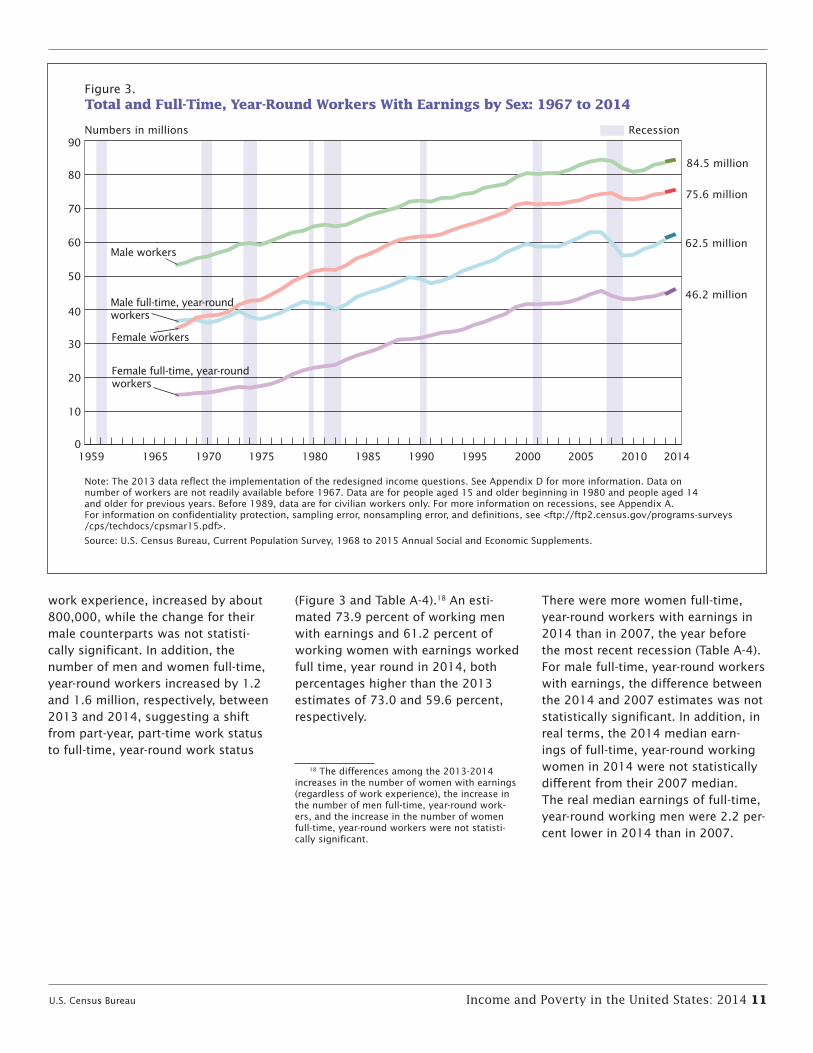
work experience, increased by about 800,000, while the change for their male counterparts was not statisti-cally significant. In addition, the number of men and women full-time, year-round workers increased by 1.2 and 1.6 million, respectively, between 2013 and 2014, suggesting a shift from part-year, part-time work status to full-time, year-round work status

(Figure 3 and Table A-4).18 An esti-mated 73.9 percent of working men with earnings and 61.2 percent of working women with earnings worked full time, year round in 2014, both percentages higher than the 2013 estimates of 73.0 and 59.6 percent, respectively.

18 The differences among the 2013-2014 increases in the number of women with earnings (regardless of work experience), the increase in the number of men full-time, year-round work-ers, and the increase in the number of women full-time, year-round workers were not statisti-cally significant.

There were more women full-time, year-round workers with earnings in 2014 than in 2007, the year before the most recent recession (Table A-4). For male full-time, year-round workers with earnings, the difference between the 2014 and 2007 estimates was not statistically significant. In addition, in real terms, the 2014 median earn-ings of full-time, year-round working women in 2014 were not statistically different from their 2007 median. The real median earnings of full-time, year-round working men were 2.2 per-cent lower in 2014 than in 2007.

Figure 3.Total and Full-Time, Year-Round Workers With Earnings by Sex: 1967 to 2014

Note: The 2013 data reflect the implementation of the redesigned income questions. See Appendix D for more information. Data on number of workers are not readily available before 1967. Data are for people aged 15 and older beginning in 1980 and people aged 14 and older for previous years. Before 1989, data are for civilian workers only. For more information on recessions, see Appendix A. For information on confidentiality protection, sampling error, nonsampling error, and definitions, see <ftp://ftp2.census.gov/programs-surveys/cps/techdocs/cpsmar15.pdf>.


Numbers in millions Recession

84.5 million

75.6 million

62.5 million

46.2 million

0

10

20

30

40

50

60

70

80

90

2014201020052000 19951990198519801975197019651959

Female full-time, year-round workers

Male workers

Female workers

Male full-time, year-round workers


POVERTY IN THE UNITED STATES 19

Highlights

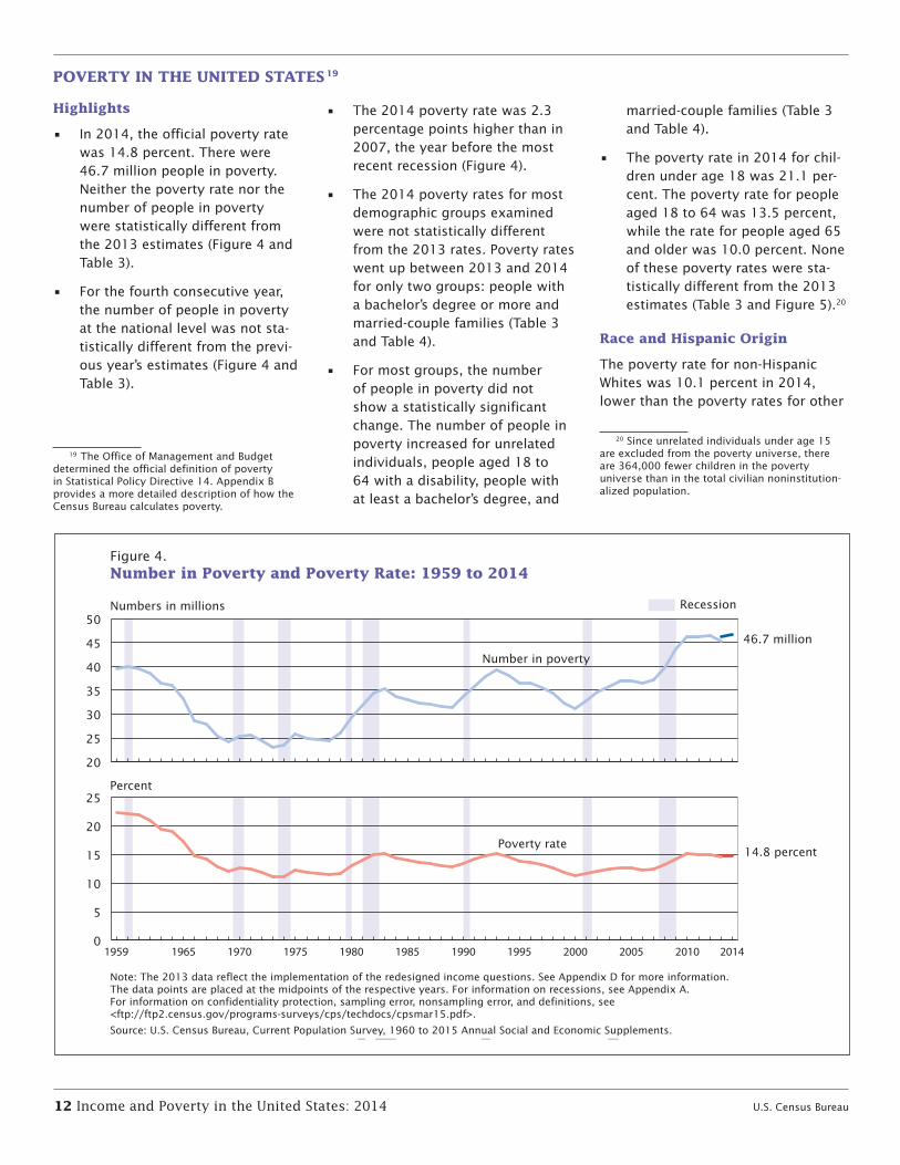
• In 2014, the official poverty rate was 14.8 percent. There were 46.7 million people in poverty. Neither the poverty rate nor the number of people in poverty were statistically different from the 2013 estimates (Figure 4 and Table 3).

• For the fourth consecutive year, the number of people in poverty at the national level was not sta-tistically different from the previ-ous year’s estimates (Figure 4 and Table 3).

19 The Office of Management and Budget determined the official definition of poverty in Statistical Policy Directive 14. Appendix B provides a more detailed description of how the Census Bureau calculates poverty.

• The 2014 poverty rate was 2.3 percentage points higher than in 2007, the year before the most recent recession (Figure 4).

• The 2014 poverty rates for most demographic groups examined were not statistically different from the 2013 rates. Poverty rates went up between 2013 and 2014 for only two groups: people with a bachelor’s degree or more and married-couple families (Table 3 and Table 4).

• For most groups, the number of people in poverty did not show a statistically significant change. The number of people in poverty increased for unrelated individuals, people aged 18 to 64 with a disability, people with at least a bachelor’s degree, and

married-couple families (Table 3 and Table 4).

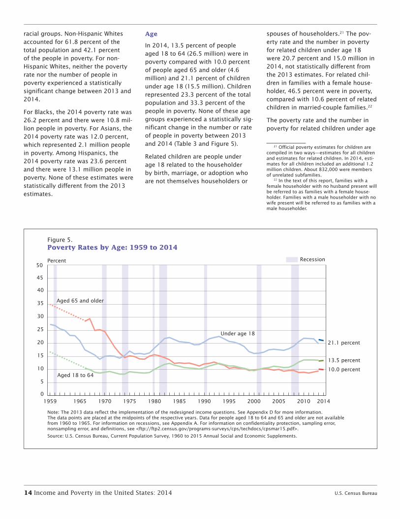
• The poverty rate in 2014 for chil-dren under age 18 was 21.1 per-cent. The poverty rate for people aged 18 to 64 was 13.5 percent, while the rate for people aged 65 and older was 10.0 percent. None of these poverty rates were sta-tistically different from the 2013 estimates (Table 3 and Figure 5).20

Race and Hispanic Origin

The poverty rate for non-Hispanic Whites was 10.1 percent in 2014, lower than the poverty rates for other

20 Since unrelated individuals under age 15 are excluded from the poverty universe, there are 364,000 fewer children in the poverty universe than in the total civilian noninstitution-alized population.

Figure 4.Number in Poverty and Poverty Rate: 1959 to 2014

Note: The 2013 data reflect the implementation of the redesigned income questions. See Appendix D for more information.The data points are placed at the midpoints of the respective years. For information on recessions, see Appendix A. For information on confidentiality protection, sampling error, nonsampling error, and definitions, see <ftp://ftp2.census.gov/programs-surveys/cps/techdocs/cpsmar15.pdf>.


Numbers in millions Recession

46.7 million

14.8 percent

Number in poverty

Poverty rate

Percent

20

25

30

35

40

45

50

0

5

10

15

20

25

2014201020052000 19951990198519801975197019651959


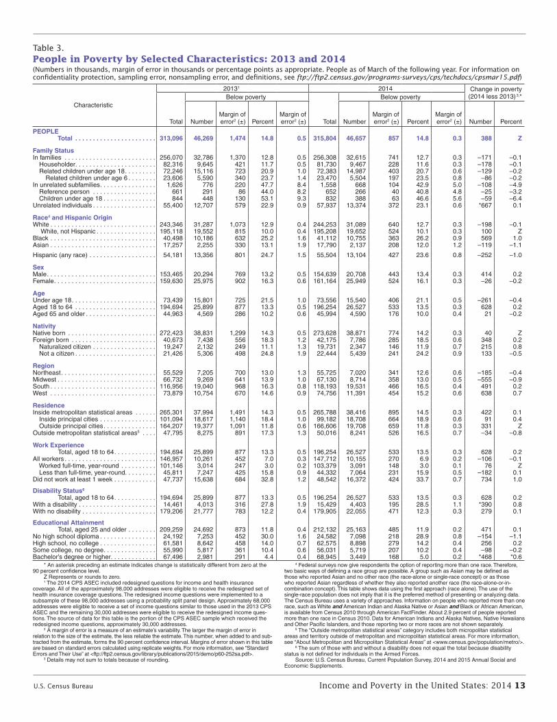
Table 3.People in Poverty by Selected Characteristics: 2013 and 2014(Numbers in thousands, margin of error in thousands or percentage points as appropriate. People as of March of the following year. For information on confidentiality protection, sampling error, nonsampling error, and definitions, see ftp://ftp2.census.gov/programs-surveys/cps/techdocs/cpsmar15.pdf)

20131 2014 Change in poverty 3,*(2014 less 2013) Below poverty Below poverty

Characteristic

Total NumberMargin of error2 (±) Percent

Margin of error2 (±) Total Number

Margin of error2 (±) Percent

Margin of error2 (±) Number Percent

PEOPLE Total . . . . . . . . . . . . . . . . . . . . . . .

Family Status

313,096 46,269 1,474 14.8 0.5 315,804 46,657 857 14.8 0.3 388 Z

In families . . . . . . . . . . . . . . . . . . . . . . . . . . 256,070 32,786 1,370 12.8 0.5 256,308 32,615 741 12.7 0.3 –171 –0.1 Householder . . . . . . . . . . . . . . . . . . . . . . . 82,316 9,645 421 11.7 0.5 81,730 9,467 228 11.6 0.3 –178 –0.1 Related children under age 18 . . . . . . . . . 72,246 15,116 723 20.9 1.0 72,383 14,987 403 20.7 0.6 –129 –0.2 Related children under age 6 . . . . . . . . 23,606 5,590 340 23.7 1.4 23,470 5,504 197 23.5 0.8 –86 –0.2In unrelated subfamilies . . . . . . . . . . . . . . . . 1,626 776 220 47.7 8.4 1,558 668 104 42.9 5.0 –108 –4.9 Reference person . . . . . . . . . . . . . . . . . . 661 291 86 44.0 8.2 652 266 40 40.8 4.8 –25 –3.2 Children under age 18 . . . . . . . . . . . . . . . 844 448 130 53.1 9.3 832 388 63 46.6 5.6 –59 –6.4Unrelated individuals . . . . . . . . . . . . . . . . . .

Race4 and Hispanic Origin

55,400 12,707 579 22.9 0.9 57,937 13,374 372 23.1 0.6 *667 0.1

White . . . . . . . . . . . . . . . . . . . . . . . . . . . . . . 243,346 31,287 1,073 12.9 0.4 244,253 31,089 640 12.7 0.3 –198 –0.1 White, not Hispanic . . . . . . . . . . . . . . . . . 195,118 19,552 815 10.0 0.4 195,208 19,652 524 10.1 0.3 100 ZBlack . . . . . . . . . . . . . . . . . . . . . . . . . . . . . . 40,498 10,186 632 25.2 1.6 41,112 10,755 363 26.2 0.9 569 1.0Asian . . . . . . . . . . . . . . . . . . . . . . . . . . . . . . 17,257 2,255 330 13.1 1.9 17,790 2,137 208 12.0 1.2 –119 –1.1

Hispanic (any race) . . . . . . . . . . . . . . . . . . .

Sex

54,181 13,356 801 24.7 1.5 55,504 13,104 427 23.6 0.8 –252 –1.0

Male . . . . . . . . . . . . . . . . . . . . . . . . . . . . . . . 153,465 20,294 769 13.2 0.5 154,639 20,708 443 13.4 0.3 414 0.2Female . . . . . . . . . . . . . . . . . . . . . . . . . . . . .

Age

159,630 25,975 902 16.3 0.6 161,164 25,949 524 16.1 0.3 –26 –0.2

Under age 18 . . . . . . . . . . . . . . . . . . . . . . . . 73,439 15,801 725 21.5 1.0 73,556 15,540 406 21.1 0.5 –261 –0.4Aged 18 to 64 . . . . . . . . . . . . . . . . . . . . . . . 194,694 25,899 877 13.3 0.5 196,254 26,527 533 13.5 0.3 628 0.2Aged 65 and older . . . . . . . . . . . . . . . . . . . .

Nativity

44,963 4,569 286 10.2 0.6 45,994 4,590 176 10.0 0.4 21 –0.2

Native born . . . . . . . . . . . . . . . . . . . . . . . . . 272,423 38,831 1,299 14.3 0.5 273,628 38,871 774 14.2 0.3 40 ZForeign born . . . . . . . . . . . . . . . . . . . . . . . . 40,673 7,438 556 18.3 1.2 42,175 7,786 285 18.5 0.6 348 0.2 Naturalized citizen . . . . . . . . . . . . . . . . . . 19,247 2,132 249 11.1 1.3 19,731 2,347 146 11.9 0.7 215 0.8 Not a citizen . . . . . . . . . . . . . . . . . . . . . . .

Region

21,426 5,306 498 24.8 1.9 22,444 5,439 241 24.2 0.9 133 –0.5

Northeast . . . . . . . . . . . . . . . . . . . . . . . . . . . 55,529 7,205 700 13.0 1.3 55,725 7,020 341 12.6 0.6 –185 –0.4Midwest . . . . . . . . . . . . . . . . . . . . . . . . . . . . 66,732 9,269 641 13.9 1.0 67,130 8,714 358 13.0 0.5 –555 –0.9South . . . . . . . . . . . . . . . . . . . . . . . . . . . . . . 116,956 19,040 968 16.3 0.8 118,193 19,531 466 16.5 0.4 491 0.2West . . . . . . . . . . . . . . . . . . . . . . . . . . . . . .

Residence

73,879 10,754 670 14.6 0.9 74,756 11,391 454 15.2 0.6 638 0.7

Inside metropolitan statistical areas . . . . . . 265,301 37,994 1,491 14.3 0.5 265,788 38,416 895 14.5 0.3 422 0.1 Inside principal cities . . . . . . . . . . . . . . . . 101,094 18,617 1,140 18.4 1.0 99,182 18,708 664 18.9 0.6 91 0.4 Outside principal cities . . . . . . . . . . . . . . . 164,207 19,377 1,091 11.8 0.6 166,606 19,708 659 11.8 0.3 331 ZOutside metropolitan statistical areas5 . . . .

Work Experience

47,795 8,275 891 17.3 1.3 50,016 8,241 526 16.5 0.7 –34 –0.8

Total, aged 18 to 64 . . . . . . . . . . . . 194,694 25,899 877 13.3 0.5 196,254 26,527 533 13.5 0.3 628 0.2All workers . . . . . . . . . . . . . . . . . . . . . . . . . . 146,957 10,261 452 7.0 0.3 147,712 10,155 270 6.9 0.2 –106 –0.1 Worked full-time, year-round . . . . . . . . . . 101,146 3,014 247 3.0 0.2 103,379 3,091 148 3.0 0.1 76 Z Less than full-time, year-round. . . . . . . . . 45,811 7,247 425 15.8 0.9 44,332 7,064 231 15.9 0.5 –182 0.1Did not work at least 1 week . . . . . . . . . . . .

Disability Status6

47,737 15,638 684 32.8 1.2 48,542 16,372 424 33.7 0.7 734 1.0

Total, aged 18 to 64 . . . . . . . . . . . . 194,694 25,899 877 13.3 0.5 196,254 26,527 533 13.5 0.3 628 0.2With a disability . . . . . . . . . . . . . . . . . . . . . . 14,461 4,013 316 27.8 1.9 15,429 4,403 195 28.5 1.1 *390 0.8With no disability . . . . . . . . . . . . . . . . . . . . .

Educational Attainment

179,206 21,777 783 12.2 0.4 179,905 22,055 471 12.3 0.3 279 0.1

Total, aged 25 and older . . . . . . . . 209,259 24,692 873 11.8 0.4 212,132 25,163 485 11.9 0.2 471 0.1No high school diploma . . . . . . . . . . . . . . . . 24,192 7,253 452 30.0 1.6 24,582 7,098 218 28.9 0.8 –154 –1.1High school, no college . . . . . . . . . . . . . . . . 61,581 8,642 458 14.0 0.7 62,575 8,898 279 14.2 0.4 256 0.2Some college, no degree . . . . . . . . . . . . . . . 55,990 5,817 361 10.4 0.6 56,031 5,719 207 10.2 0.4 –98 –0.2Bachelor’s degree or higher . . . . . . . . . . . . . 67,496 2,981 291 4.4 0.4 68,945 3,449 168 5.0 0.2 *468 *0.6

* An asterisk preceding an estimate indicates change is statistically different from zero at the 90 percent confidence level.

Z Represents or rounds to zero. 1 The 2014 CPS ASEC included redesigned questions for income and health insurance

coverage. All of the approximately 98,000 addresses were eligible to receive the redesigned set of health insurance coverage questions. The redesigned income questions were implemented to a subsample of these 98,000 addresses using a probability split panel design. Approximately 68,000 addresses were eligible to receive a set of income questions similar to those used in the 2013 CPS ASEC and the remaining 30,000 addresses were eligible to receive the redesigned income ques-tions. The source of data for this table is the portion of the CPS ASEC sample which received the redesigned income questions, approximately 30,000 addresses.

2 A margin of error is a measure of an estimate’s variability. The larger the margin of error in relation to the size of the estimate, the less reliable the estimate. This number, when added to and sub-tracted from the estimate, forms the 90 percent confidence interval. Margins of error shown in this table are based on standard errors calculated using replicate weights. For more information, see “Standard Errors and Their Use” at <ftp://ftp2.census.gov/library/publications/2015/demo/p60-252sa.pdf>.

3 Details may not sum to totals because of rounding.

4 Federal surveys now give respondents the option of reporting more than one race. Therefore, two basic ways of defining a race group are possible. A group such as Asian may be defined as those who reported Asian and no other race (the race-alone or single-race concept) or as those who reported Asian regardless of whether they also reported another race (the race-alone-or-in- combination concept). This table shows data using the first approach (race alone). The use of the single-race population does not imply that it is the preferred method of presenting or analyzing data. The Census Bureau uses a variety of approaches. Information on people who reported more than one race, such as White and American Indian and Alaska Native or Asian and Black or African American, is available from Census 2010 through American FactFinder. About 2.9 percent of people reported more than one race in Census 2010. Data for American Indians and Alaska Natives, Native Hawaiians and Other Pacific Islanders, and those reporting two or more races are not shown separately.

5 The “Outside metropolitan statistical areas” category includes both micropolitan statistical areas and territory outside of metropolitan and micropolitan statistical areas. For more information, see “About Metropolitan and Micropolitan Statistical Areas” at <www.census.gov/population/metro/>.

6 The sum of those with and without a disability does not equal the total because disability status is not defined for individuals in the Armed Forces.

Source: U.S. Census Bureau, Current Population Survey, 2014 and 2015 Annual Social and Economic Supplements.


racial groups. Non-Hispanic Whites accounted for 61.8 percent of the total population and 42.1 percent of the people in poverty. For non- Hispanic Whites, neither the poverty rate nor the number of people in poverty experienced a statistically significant change between 2013 and 2014.

For Blacks, the 2014 poverty rate was 26.2 percent and there were 10.8 mil-lion people in poverty. For Asians, the 2014 poverty rate was 12.0 percent, which represented 2.1 million people in poverty. Among Hispanics, the 2014 poverty rate was 23.6 percent and there were 13.1 million people in poverty. None of these estimates were statistically different from the 2013 estimates.

Age

In 2014, 13.5 percent of people aged 18 to 64 (26.5 million) were in poverty compared with 10.0 percent of people aged 65 and older (4.6 million) and 21.1 percent of children under age 18 (15.5 million). Children represented 23.3 percent of the total population and 33.3 percent of the people in poverty. None of these age groups experienced a statistically sig-nificant change in the number or rate of people in poverty between 2013 and 2014 (Table 3 and Figure 5).

Related children are people under age 18 related to the householder by birth, marriage, or adoption who are not themselves householders or

spouses of householders.21 The pov-erty rate and the number in poverty for related children under age 18 were 20.7 percent and 15.0 million in 2014, not statistically different from the 2013 estimates. For related chil-dren in families with a female house-holder, 46.5 percent were in poverty, compared with 10.6 percent of related children in married-couple families.22

The poverty rate and the number in poverty for related children under age

21 Official poverty estimates for children are compiled in two ways—estimates for all children and estimates for related children. In 2014, esti-mates for all children included an additional 1.2 million children. About 832,000 were members of unrelated subfamilies.

22 In the text of this report, families with a female householder with no husband present will be referred to as families with a female house-holder. Families with a male householder with no wife present will be referred to as families with a male householder.

Figure 5.Poverty Rates by Age: 1959 to 2014

Note: The 2013 data reflect the implementation of the redesigned income questions. See Appendix D for more information.The data points are placed at the midpoints of the respective years. Data for people aged 18 to 64 and 65 and older are not available from 1960 to 1965. For information on recessions, see Appendix A. For information on confidentiality protection, sampling error, nonsampling error, and definitions, see <ftp://ftp2.census.gov/programs-surveys/cps/techdocs/cpsmar15.pdf>.


Percent

0

5

10

15

20

25

30

35

40

45

50

2014201020052000 19951990198519801975197019651959

Recession

13.5 percent

10.0 percent

21.1 percent

Aged 18 to 64

Under age 18

Aged 65 and older


6 were 23.5 percent and 5.5 million in 2014, not statistically different from the 2013 estimates. About 1 in 5 of these children were in poverty in 2014. More than half (55.1 percent) of related children under age 6 in families with a female householder were in poverty. This was more than four times the rate of their counter-parts in married-couple families (11.6 percent).

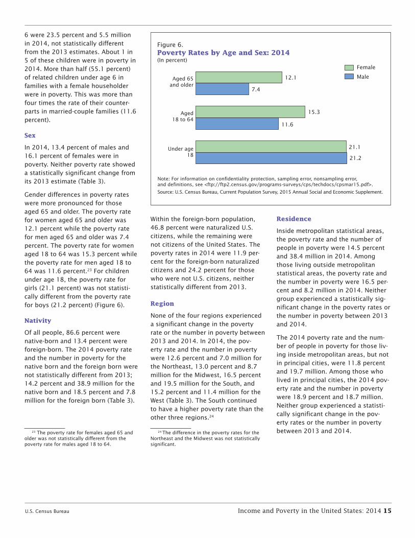
Sex

In 2014, 13.4 percent of males and 16.1 percent of females were in poverty. Neither poverty rate showed a statistically significant change from its 2013 estimate (Table 3).

Gender differences in poverty rates were more pronounced for those aged 65 and older. The poverty rate for women aged 65 and older was 12.1 percent while the poverty rate for men aged 65 and older was 7.4 percent. The poverty rate for women aged 18 to 64 was 15.3 percent while the poverty rate for men aged 18 to 64 was 11.6 percent.23 For children under age 18, the poverty rate for girls (21.1 percent) was not statisti-cally different from the poverty rate for boys (21.2 percent) (Figure 6).

Nativity

Of all people, 86.6 percent were native-born and 13.4 percent were foreign-born. The 2014 poverty rate and the number in poverty for the native born and the foreign born were not statistically different from 2013; 14.2 percent and 38.9 million for the native born and 18.5 percent and 7.8 million for the foreign born (Table 3).

23 The poverty rate for females aged 65 and older was not statistically different from the poverty rate for males aged 18 to 64.

Within the foreign-born population, 46.8 percent were naturalized U.S. citizens, while the remaining were not citizens of the United States. The poverty rates in 2014 were 11.9 per-cent for the foreign-born naturalized citizens and 24.2 percent for those who were not U.S. citizens, neither statistically different from 2013.

Region

None of the four regions experienced a significant change in the poverty rate or the number in poverty between 2013 and 2014. In 2014, the pov-erty rate and the number in poverty were 12.6 percent and 7.0 million for the Northeast, 13.0 percent and 8.7 million for the Midwest, 16.5 percent and 19.5 million for the South, and 15.2 percent and 11.4 million for the West (Table 3). The South continued to have a higher poverty rate than the other three regions.24

24 The difference in the poverty rates for the Northeast and the Midwest was not statistically significant.

Residence

Inside metropolitan statistical areas, the poverty rate and the number of people in poverty were 14.5 percent and 38.4 million in 2014. Among those living outside metropolitan statistical areas, the poverty rate and the number in poverty were 16.5 per-cent and 8.2 million in 2014. Neither group experienced a statistically sig-nificant change in the poverty rates or the number in poverty between 2013 and 2014.

The 2014 poverty rate and the num-ber of people in poverty for those liv-ing inside metropolitan areas, but not in principal cities, were 11.8 percent and 19.7 million. Among those who lived in principal cities, the 2014 pov-erty rate and the number in poverty were 18.9 percent and 18.7 million. Neither group experienced a statisti-cally significant change in the pov-erty rates or the number in poverty between 2013 and 2014.

Figure 6.Poverty Rates by Age and Sex: 2014(In percent)

Female

Male

21.1

21.2

15.3

7.4

12.1

11.6

Under age18

Aged18 to 64

Aged 65and older

Note: For information on confidentiality protection, sampling error, nonsampling error, and definitions, see <ftp://ftp2.census.gov/programs-surveys/cps/techdocs/cpsmar15.pdf>.

Source: U.S. Census Bureau, Current Population Survey, 2015 Annual Social and Economic Supplement.


Within metropolitan areas, people in poverty were more likely to live in principal cities in 2014. While 37.3 percent of all people living in metro-politan areas lived in principal cities, 48.7 percent of poor people in met-ropolitan areas lived in principal cities (Table 3).

Work Experience

In 2014, 6.9 percent of workers aged 18 to 64 were in poverty. The poverty rate for those who worked full time, year round was 3.0 percent, while the poverty rate for those working less than full time, year round was 15.9 percent. None of these rates were statistically different from the 2013 poverty rates (Table 3).

Among those who did not work at least 1 week in 2014, the poverty rate and the number in poverty were 33.7 percent and 16.4 million in 2014, not statistically different from the 2013 estimates (Table 3). Those who did not work in 2014 represented 24.7 percent of all people aged 18 to 64, compared with 61.7 percent of people aged 18 to 64 in poverty.

Disability Status

In 2014, for people aged 18 to 64 with a disability, the poverty rate was 28.5 percent, not statistically different from 2013, whereas the number of people aged 18 to 64 with a disability increased from 4.0 million in 2013 to 4.4 million 2014. For people aged 18 to 64 without a disability, the poverty rate and number in poverty were 12.3 percent and 22.1 million, neither sta-tistically different from the previous year estimates.

Among people aged 18 to 64, those with a disability represented 7.9 percent of all people compared with 16.6 percent of people aged 18 to 64 in poverty.

Educational Attainment

In 2014, 28.9 percent of people aged 25 and older without a high school diploma were in poverty. The pov-erty rate for those with a high school diploma but with no college was 14.2 percent, while the poverty rate for those with some college but no degree was 10.2 percent. None of

these rates were statistically different from the 2013 poverty rates (Table 3).

Among people with at least a bach-elor’s degree, the poverty rate and the number in poverty were 5.0 percent and 3.4 million in 2014, up from 4.4 percent and 3.0 million in 2013 (Table 3). People with at least a bache-lor’s degree in 2014 represented 32.5 percent of all people aged 25 and older, compared with 13.7 percent of people aged 25 and older in poverty.

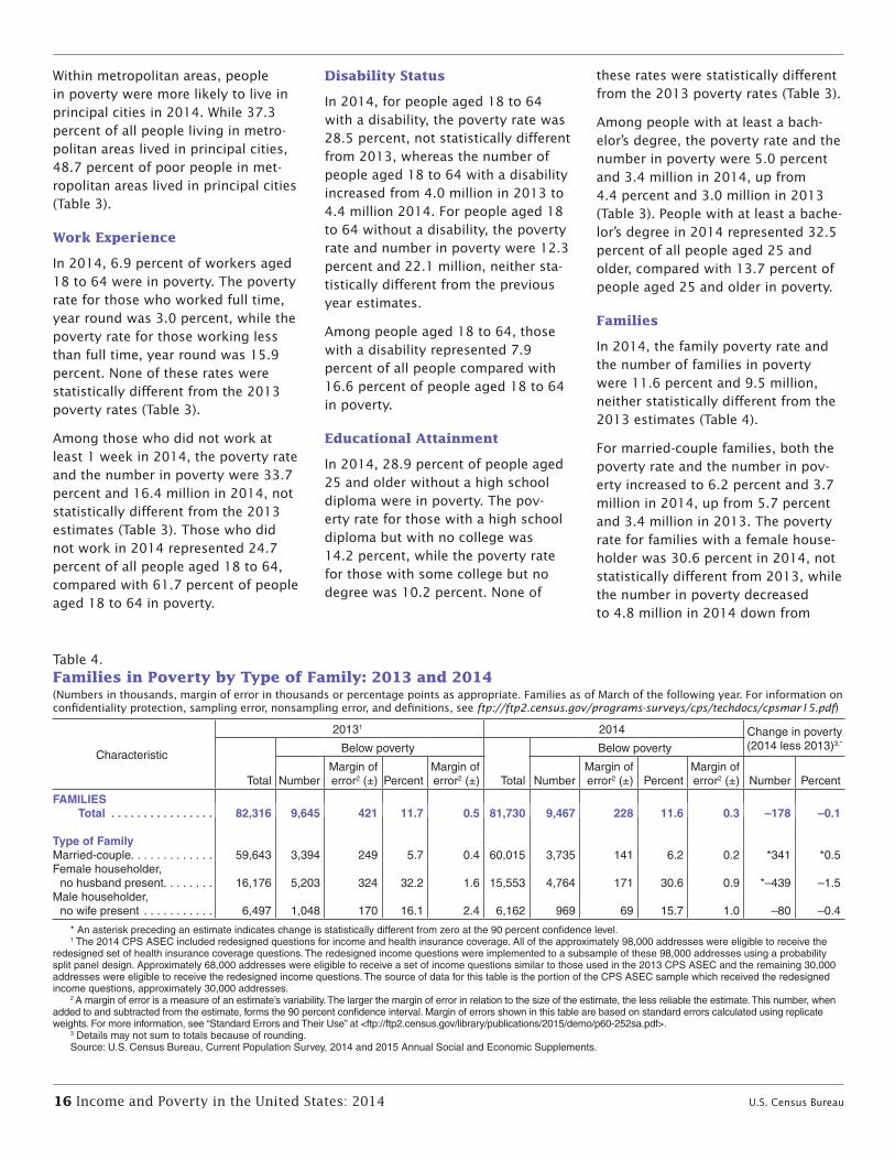
Families

In 2014, the family poverty rate and the number of families in poverty were 11.6 percent and 9.5 million, neither statistically different from the 2013 estimates (Table 4).

For married-couple families, both the poverty rate and the number in pov-erty increased to 6.2 percent and 3.7 million in 2014, up from 5.7 percent and 3.4 million in 2013. The poverty rate for families with a female house-holder was 30.6 percent in 2014, not statistically different from 2013, while the number in poverty decreased to 4.8 million in 2014 down from

Table 4.Families in Poverty by Type of Family: 2013 and 2014(Numbers in thousands, margin of error in thousands or percentage points as appropriate. Families as of March of the following year. For information on confidentiality protection, sampling error, nonsampling error, and definitions, see ftp://ftp2.census.gov/programs-surveys/cps/techdocs/cpsmar15.pdf)

Characteristic

20131 2014 Change in poverty (2014 less 2013)3,*

Total

Below poverty

Total

Below poverty

NumberMargin of error2 (±) Percent

Margin of error2 (±) Number

Margin of error2 (±) Percent

Margin of error2 (±) Number Percent

FAMILIES Total . . . . . . . . . . . . . . . . 82,316 9,645 421 11.7 0.5 81,730 9,467 228 11.6 0.3 –178 –0.1

Type of FamilyMarried-couple. . . . . . . . . . . . . 59,643 3,394 249 5.7 0.4 60,015 3,735 141 6.2 0.2 *341 *0.5Female householder,

no husband present. . . . . . . . 16,176 5,203 324 32.2 1.6 15,553 4,764 171 30.6 0.9 *–439 –1.5Male householder,

no wife present . . . . . . . . . . . 6,497 1,048 170 16.1 2.4 6,162 969 69 15.7 1.0 –80 –0.4

* An asterisk preceding an estimate indicates change is statistically different from zero at the 90 percent confidence level.1 The 2014 CPS ASEC included redesigned questions for income and health insurance coverage. All of the approximately 98,000 addresses were eligible to receive the

redesigned set of health insurance coverage questions. The redesigned income questions were implemented to a subsample of these 98,000 addresses using a probability split panel design. Approximately 68,000 addresses were eligible to receive a set of income questions similar to those used in the 2013 CPS ASEC and the remaining 30,000 addresses were eligible to receive the redesigned income questions. The source of data for this table is the portion of the CPS ASEC sample which received the redesigned income questions, approximately 30,000 addresses.

2 A margin of error is a measure of an estimate’s variability. The larger the margin of error in relation to the size of the estimate, the less reliable the estimate. This number, when added to and subtracted from the estimate, forms the 90 percent confidence interval. Margin of errors shown in this table are based on standard errors calculated using replicate weights. For more information, see “Standard Errors and Their Use” at <ftp://ftp2.census.gov/library/publications/2015/demo/p60-252sa.pdf>.

3 Details may not sum to totals because of rounding.Source: U.S. Census Bureau, Current Population Survey, 2014 and 2015 Annual Social and Economic Supplements.


5.2 million in 2013. For families with a male householder, neither the poverty rate nor the number in poverty showed any statistical change between 2013 and 2014. For families with a male householder, 15.7 percent were in poverty in 2014. This repre-sented 1.0 million families in 2014.

Depth of Poverty

Categorizing a person as “in poverty” or “not in poverty” is one way to describe his or her economic situa-tion. The income-to-poverty ratio and the income deficit or surplus describe additional aspects of economic well-being. While the poverty rate shows the proportion of people with income below the relevant poverty threshold,

the income-to-poverty ratio gauges the depth of poverty and shows how close a family’s income is to its pov-erty threshold. The income-to-poverty ratio is reported as a percentage that compares a family’s or an unrelated person’s income with the applicable threshold. For example, a family with an income-to-poverty ratio of 125 percent has income that is 25 percent above its poverty threshold.

The income deficit or surplus shows how many dollars a family’s or an indi-vidual’s income is below (or above) their poverty threshold. For those with an income deficit, the measure is an estimate of the dollar amount nec-essary to raise a family’s or a person’s income to their poverty threshold.

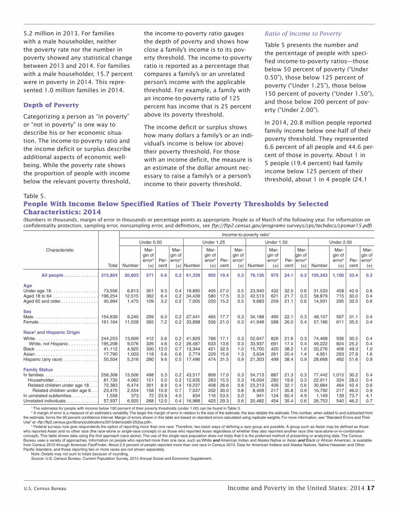
Ratio of Income to Poverty

Table 5 presents the number and the percentage of people with speci-fied income-to-poverty ratios—those below 50 percent of poverty (“Under 0.50”), those below 125 percent of poverty (“Under 1.25”), those below 150 percent of poverty (“Under 1.50”), and those below 200 percent of pov-erty (“Under 2.00”).

In 2014, 20.8 million people reported family income below one-half of their poverty threshold. They represented 6.6 percent of all people and 44.6 per-cent of those in poverty. About 1 in 5 people (19.4 percent) had family income below 125 percent of their threshold, about 1 in 4 people (24.1

Table 5.People With Income Below Specified Ratios of Their Poverty Thresholds by Selected Characteristics: 2014(Numbers in thousands, margin of error in thousands or percentage points as appropriate. People as of March of the following year. For information on confidentiality protection, sampling error, nonsampling error, and definitions, see ftp://ftp2.census.gov/programs-surveys/cps/techdocs/cpsmar15.pdf)

Characteristic

Total

Income-to-poverty ratio1

Under 0.50 Under 1.25 Under 1.50 Under 2.00

Number

Mar-gin of error2

(±)Per-cent

Mar-gin of error2

(±) Number

Mar-gin of error2

(±)Per-cent

Mar-gin of error2

(±) Number

Mar-gin of error2

(±)Per-cent

Mar-gin of error2

(±) Number

Mar-gin of error2

(±)Per-cent

Mar-gin of error2

(±)

All people . . . . . . . . . . . . . . 315,804 20,803 571 6.6 0.2 61,339 905 19.4 0.3 76,135 975 24.1 0.3 105,343 1,100 33.4 0.3

AgeUnder age 18 . . . . . . . . . . . . . . . . . . . 73,556 6,813 301 9.3 0.4 19,895 405 27.0 0.5 23,940 432 32.5 0.6 31,533 458 42.9 0.6Aged 18 to 64 . . . . . . . . . . . . . . . . . . 196,254 12,515 362 6.4 0.2 34,439 580 17.5 0.3 42,513 621 21.7 0.3 58,879 715 30.0 0.4Aged 65 and older . . . . . . . . . . . . . . . 45,994 1,475 109 3.2 0.2 7,005 220 15.2 0.5 9,683 259 21.1 0.6 14,931 295 32.5 0.6

SexMale . . . . . . . . . . . . . . . . . . . . . . . . . . 154,639 9,245 299 6.0 0.2 27,441 465 17.7 0.3 34,188 495 22.1 0.3 48,157 597 31.1 0.4Female . . . . . . . . . . . . . . . . . . . . . . . . 161,164 11,558 365 7.2 0.2 33,898 556 21.0 0.3 41,948 588 26.0 0.4 57,186 611 35.5 0.4

Race3 and Hispanic OriginWhite . . . . . . . . . . . . . . . . . . . . . . . . . 244,253 13,609 412 5.6 0.2 41,829 766 17.1 0.3 52,647 826 21.6 0.3 74,468 936 30.5 0.4 White, not Hispanic . . . . . . . . . . . . 195,208 9,076 326 4.6 0.2 26,487 633 13.6 0.3 33,937 691 17.4 0.4 49,222 824 25.2 0.4Black . . . . . . . . . . . . . . . . . . . . . . . . . 41,112 4,925 300 12.0 0.7 13,344 421 32.5 1.0 15,700 420 38.2 1.0 20,276 406 49.3 1.0Asian . . . . . . . . . . . . . . . . . . . . . . . . . 17,790 1,003 118 5.6 0.6 2,774 229 15.6 1.3 3,634 261 20.4 1.4 4,951 293 27.8 1.6Hispanic (any race) . . . . . . . . . . . . . . 55,504 5,316 280 9.6 0.5 17,496 474 31.5 0.9 21,303 499 38.4 0.9 28,668 492 51.6 0.9

Family StatusIn families . . . . . . . . . . . . . . . . . . . . . 256,308 13,506 498 5.3 0.2 43,517 809 17.0 0.3 54,713 887 21.3 0.3 77,442 1,015 30.2 0.4 Householder . . . . . . . . . . . . . . . . . . 81,730 4,062 151 5.0 0.2 12,635 263 15.5 0.3 16,004 282 19.6 0.3 22,911 324 28.0 0.4 Related children under age 18 . . . . 72,383 6,474 301 8.9 0.4 19,237 408 26.6 0.6 23,213 439 32.1 0.6 30,684 464 42.4 0.6 Related children under age 6 . . . 23,470 2,554 158 10.9 0.7 7,037 202 30.0 0.8 8,409 217 35.8 0.9 10,792 217 46.0 0.9In unrelated subfamilies . . . . . . . . . . . 1,558 373 72 23.9 4.0 834 116 53.5 5.0 941 124 60.4 4.9 1,149 139 73.7 4.1Unrelated individuals . . . . . . . . . . . . . 57,937 6,925 268 12.0 0.4 16,988 425 29.3 0.6 20,482 454 35.4 0.6 26,753 540 46.2 0.7

1 The estimates for people with income below 100 percent of their poverty thresholds (under 1.00) can be found in Table 3.2 A margin of error is a measure of an estimate’s variability. The larger the margin of error in relation to the size of the estimate, the less reliable the estimate. This number, when added to and subtracted from

the estimate, forms the 90 percent confidence interval. Margin of errors shown in this table are based on standard errors calculated using replicate weights. For more information, see “Standard Errors and Their Use” at <ftp://ftp2.census.gov/library/publications/2015/demo/p60-252sa.pdf>.

3 Federal surveys now give respondents the option of reporting more than one race. Therefore, two basic ways of defining a race group are possible. A group such as Asian may be defined as those who reported Asian and no other race (the race-alone or single-race concept) or as those who reported Asian regardless of whether they also reported another race (the race-alone-or-in-combination concept). This table shows data using the first approach (race alone). The use of the single-race population does not imply that it is the preferred method of presenting or analyzing data. The Census Bureau uses a variety of approaches. Information on people who reported more than one race, such as White and American Indian and Alaska Native or Asian and Black or African American, is available from Census 2010 through American FactFinder. About 2.9 percent of people reported more than one race in Census 2010. Data for American Indians and Alaska Natives, Native Hawaiian and Other Pacific Islanders, and those reporting two or more races are not shown separately.

Note: Details may not sum to totals because of rounding.Source: U.S. Census Bureau, Current Population Survey, 2015 Annual Social and Economic Supplement.


percent) had family income below 150 percent of their poverty thresh-old, while approximately 1 in 3 (33.4 percent) had family income below 200 percent of their threshold (Table 5).

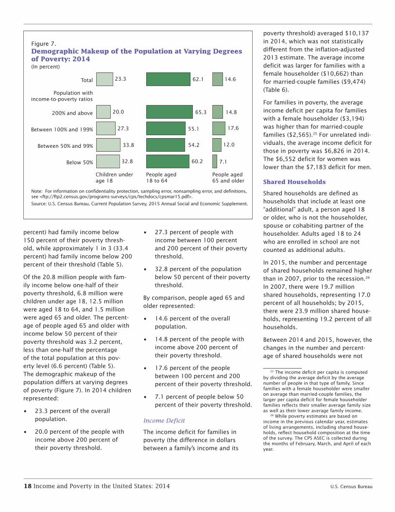
Of the 20.8 million people with fam-ily income below one-half of their poverty threshold, 6.8 million were children under age 18, 12.5 million were aged 18 to 64, and 1.5 million were aged 65 and older. The percent-age of people aged 65 and older with income below 50 percent of their poverty threshold was 3.2 percent, less than one-half the percentage of the total population at this pov-erty level (6.6 percent) (Table 5). The demographic makeup of the population differs at varying degrees of poverty (Figure 7). In 2014 children represented:

• 23.3 percent of the overall population.

• 20.0 percent of the people with income above 200 percent of their poverty threshold.

• 27.3 percent of people with income between 100 percent and 200 percent of their poverty threshold.

• 32.8 percent of the population below 50 percent of their poverty threshold.

By comparison, people aged 65 and older represented:

• 14.6 percent of the overall population.

• 14.8 percent of the people with income above 200 percent of their poverty threshold.

• 17.6 percent of the people between 100 percent and 200 percent of their poverty threshold.

• 7.1 percent of people below 50 percent of their poverty threshold.

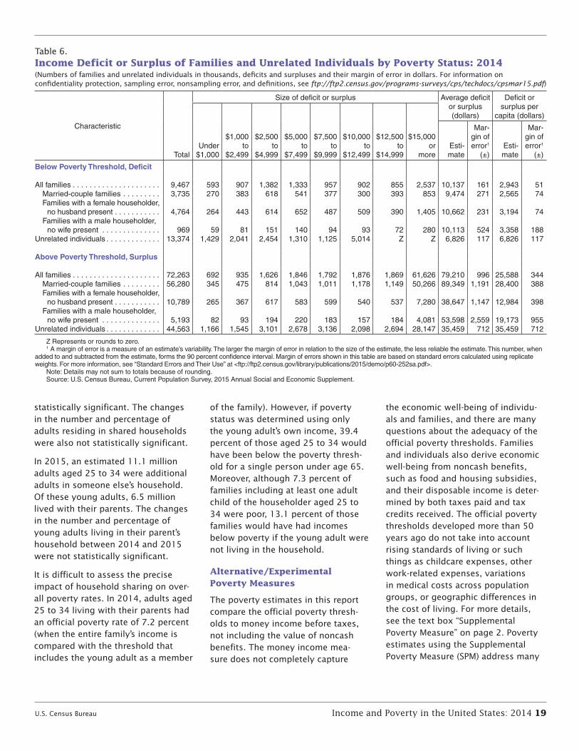
Income Deficit

The income deficit for families in poverty (the difference in dollars between a family’s income and its

poverty threshold) averaged $10,137 in 2014, which was not statistically different from the inflation-adjusted 2013 estimate. The average income deficit was larger for families with a female householder ($10,662) than for married-couple families ($9,474) (Table 6).

For families in poverty, the average income deficit per capita for families with a female householder ($3,194) was higher than for married-couple families ($2,565).25 For unrelated indi-viduals, the average income deficit for those in poverty was $6,826 in 2014. The $6,552 deficit for women was lower than the $7,183 deficit for men.

Shared Households

Shared households are defined as households that include at least one “additional” adult, a person aged 18 or older, who is not the householder, spouse or cohabiting partner of the householder. Adults aged 18 to 24 who are enrolled in school are not counted as additional adults.

In 2015, the number and percentage of shared households remained higher than in 2007, prior to the recession.26 In 2007, there were 19.7 million shared households, representing 17.0 percent of all households; by 2015, there were 23.9 million shared house-holds, representing 19.2 percent of all households.

Between 2014 and 2015, however, the changes in the number and percent-age of shared households were not

25 The income deficit per capita is computed by dividing the average deficit by the average number of people in that type of family. Since families with a female householder were smaller on average than married-couple families, the larger per capita deficit for female householder families reflects their smaller average family size as well as their lower average family income.

26 While poverty estimates are based on income in the previous calendar year, estimates of living arrangements, including shared house-holds, reflect household composition at the time of the survey. The CPS ASEC is collected during the months of February, March, and April of each year.

Figure 7.Demographic Makeup of the Population at Varying Degrees of Poverty: 2014

Below 50%

Between 50% and 99%

Between 100% and 199%

200% and above

Population with income-to-poverty ratios

Total

Children underage 18

(In percent)

23.3 62.1 14.6

65.3 14.8

17.6

12.0

7.1

55.1

54.2

60.2

20.0

27.3

33.8

32.8

People aged 18 to 64

People aged 65 and older

Note: For information on confidentiality protection, sampling error, nonsampling error, and definitions, see <ftp://ftp2.census.gov/programs-surveys/cps/techdocs/cpsmar15.pdf>.

Source: U.S. Census Bureau, Current Population Survey, 2015 Annual Social and Economic Supplement.


statistically significant. The changes in the number and percentage of adults residing in shared households were also not statistically significant.

In 2015, an estimated 11.1 million adults aged 25 to 34 were additional adults in someone else’s household. Of these young adults, 6.5 million lived with their parents. The changes in the number and percentage of young adults living in their parent’s household between 2014 and 2015 were not statistically significant.

It is difficult to assess the precise impact of household sharing on over-all poverty rates. In 2014, adults aged 25 to 34 living with their parents had an official poverty rate of 7.2 percent (when the entire family’s income is compared with the threshold that includes the young adult as a member

of the family). However, if poverty status was determined using only the young adult’s own income, 39.4 percent of those aged 25 to 34 would have been below the poverty thresh-old for a single person under age 65. Moreover, although 7.3 percent of families including at least one adult child of the householder aged 25 to 34 were poor, 13.1 percent of those families would have had incomes below poverty if the young adult were not living in the household.

Alternative/Experimental Poverty Measures

The poverty estimates in this report compare the official poverty thresh-olds to money income before taxes, not including the value of noncash benefits. The money income mea-sure does not completely capture

the economic well-being of individu-als and families, and there are many questions about the adequacy of the official poverty thresholds. Families and individuals also derive economic well-being from noncash benefits, such as food and housing subsidies, and their disposable income is deter-mined by both taxes paid and tax credits received. The official poverty thresholds developed more than 50 years ago do not take into account rising standards of living or such things as childcare expenses, other work-related expenses, variations in medical costs across population groups, or geographic differences in the cost of living. For more details, see the text box “Supplemental Poverty Measure” on page 2. Poverty estimates using the Supplemental Poverty Measure (SPM) address many

Table 6.Income Deficit or Surplus of Families and Unrelated Individuals by Poverty Status: 2014(Numbers of families and unrelated individuals in thousands, deficits and surpluses and their margin of error in dollars. For information on confidentiality protection, sampling error, nonsampling error, and definitions, see ftp://ftp2.census.gov/programs-surveys/cps/techdocs/cpsmar15.pdf)

Characteristic

Total

Size of deficit or surplus Average deficit or surplus (dollars)

Deficit or surplus per

capita (dollars)

Under$1,000

$1,000 to

$2,499

$2,500 to

$4,999

$5,000 to

$7,499

$7,500 to

$9,999

$10,000 to

$12,499

$12,500 to

$14,999

$15,000 or

moreEsti-mate

Mar-gin of error1

(±)Esti-mate

Mar-gin of error1

(±)

Below Poverty Threshold, Deficit

All families . . . . . . . . . . . . . . . . . . . . . 9,467 593 907 1,382 1,333 957 902 855 2,537 10,137 161 2,943 51 Married-couple families . . . . . . . . . 3,735 270 383 618 541 377 300 393 853 9,474 271 2,565 74 Families with a female householder,

no husband present . . . . . . . . . . . 4,764 264 443 614 652 487 509 390 1,405 10,662 231 3,194 74 Families with a male householder,

no wife present . . . . . . . . . . . . . . 969 59 81 151 140 94 93 72 280 10,113 524 3,358 188Unrelated individuals . . . . . . . . . . . . . 13,374 1,429 2,041 2,454 1,310 1,125 5,014 Z Z 6,826 117 6,826 117

Above Poverty Threshold, Surplus

All families . . . . . . . . . . . . . . . . . . . . . 72,263 692 935 1,626 1,846 1,792 1,876 1,869 61,626 79,210 996 25,588 344 Married-couple families . . . . . . . . . 56,280 345 475 814 1,043 1,011 1,178 1,149 50,266 89,349 1,191 28,400 388 Families with a female householder,

no husband present . . . . . . . . . . . 10,789 265 367 617 583 599 540 537 7,280 38,647 1,147 12,984 398 Families with a male householder,

no wife present . . . . . . . . . . . . . . 5,193 82 93 194 220 183 157 184 4,081 53,598 2,559 19,173 955Unrelated individuals . . . . . . . . . . . . . 44,563 1,166 1,545 3,101 2,678 3,136 2,098 2,694 28,147 35,459 712 35,459 712

Z Represents or rounds to zero.1 A margin of error is a measure of an estimate’s variability. The larger the margin of error in relation to the size of the estimate, the less reliable the estimate. This number, when

added to and subtracted from the estimate, forms the 90 percent confidence interval. Margin of errors shown in this table are based on standard errors calculated using replicate weights. For more information, see “Standard Errors and Their Use” at <ftp://ftp2.census.gov/library/publications/2015/demo/p60-252sa.pdf>.

Note: Details may not sum to totals because of rounding.Source: U.S. Census Bureau, Current Population Survey, 2015 Annual Social and Economic Supplement.


of these concerns. For more informa-tion on SPM estimates for 2014 see <ftp://ftp2.census.gov/library /publications/2015/demo/p60-254 .pdf>.

National Academy of Sciences (NAS)-Based Measures

The Census Bureau also computes alternative poverty measures based on the 1995 recommendations of the National Academy of Sciences Panel on Poverty and Family Assistance. The NAS-based measures, which use both alternative poverty thresholds and an expanded income definition, provide a consistent time series available from 1999 to the present (www.census .gov/prod/2001pubs/p60-216.pdf).27 The estimates for 2013 for the NAS-based measures can be found at <www.census.gov/hhes/povmeas /data/nas/tables/2013/index.html>.

Research Files

The Census Bureau makes available microdata research files that provide the variables used to construct SPM estimates and NAS-based alternative measures at <www.census.gov/hhes /povmeas/data/public-use.html>. An expanded version of the CPS ASEC public use file includes estimates

27 However, many of the elements of these measures are no longer being updated.

of the value of taxes and noncash benefits at <http://thedataweb.rm .census.gov/ftp/cps_ftp.html>.

CPS Table Creator

CPS Table Creator is a Web-based tool designed to help researchers explore alternative income and poverty mea-sures. The tool is available from a link on the Census Bureau’s poverty Web site at <www.census.gov/cps/data /cpstablecreator.html>. Table Creator allows researchers to produce pov-erty and income estimates using their own combinations of threshold and resource definitions and to see the incremental impact of the addition or subtraction of a single resource element.

Researchers can also estimate pov-erty rates using alternative poverty thresholds. Many other countries use relative poverty measures with thresh-olds that are based on a percentage of median or mean income.28 The Table Creator allows researchers to estimate poverty rates using a relative poverty threshold calculated as any percent-age of mean or median equivalence-

28 For example, the Organization for Economic Cooperation and Development (OECD) uses a poverty threshold of 50 percent of median income. The European Union defines poverty as an income below 60 percent of the national median equalized disposable income after social transfers.

adjusted income. For example, using poverty thresholds based on 50 percent of median income rather than the official poverty thresholds would increase the overall poverty rate from 14.8 percent to 22.6 percent in 2013.

COMMENTS

The Census Bureau welcomes the comments and advice of data and report users. If you have suggestions or comments on the income data, please write to:

Edward J. Welniak, Jr. Chief, Income Statistics Branch Social, Economic, and Housing Statistics Division U.S. Census Bureau Washington, D.C. 20233-8500

Or send e-mail to: [email protected]

If you have suggestions or comments on the poverty data, please write to:

Trudi J. Renwick Chief, Poverty Statistics Branch Social, Economic, and Housing Statistics Division U.S. Census Bureau Washington, D.C. 20233-8500

Or send e-mail to: [email protected]

Income and Poverty in the United States: 2014 - …and+poverty+in+the+US.pdfU.S. Census Bureau...

Documents

Transcript of Income and Poverty in the United States: 2014 - …and+poverty+in+the+US.pdfU.S. Census Bureau...