Income and Efficiency in Incomplete Markets

by Anil Arya †

John Fellingham † Jonathan Glover † † Doug Schroeder † Richard Young †

April 1996

† Ohio State University † † Carnegie Mellon University

Income and Efficiency in Incomplete Markets

1. Introduction

Aggregation is central to accounting. Vast quantities of data are reduced to a

handful of numbers. Attempts are made to capture the entire financial activity of an

entity during a period in one number - income. A legitimate question to ask is how much

useful information can be conveyed by income. The answer must depend on the context.

What questions are we using the income number to resolve?

In this paper we examine a simple but suggestive setting in which the income

number arises naturally (and directly) from competitive markets. While no explicit

assumptions are made about individual firm's objectives, it turns out that equilibrium is

consistent with the maximization of a number which is equal to the difference between

the value of commodities sold and the value of resources purchased. 1 This number,

which we call income, is instructive about the central economic questions of equilibrium

and productive efficiency in the following way.

1. If any firm's income is not maximized the economy is not in equilibrium.2

2. Given equilibrium prices, if each firm's income is maximized production is

efficient.

Forging links between an income number, equilibrium and efficiency is important

in establishing that income measurement is an interesting and useful activity. For our

1 This differs from the approach in Beaver and Demski (1995), who assume firms

maximize net present value of cash flows. 2 Our model is essentially timeless -- there is no interest rate. Also, we do not model

uncertainty, so not only is expected income zero, but so is realized income.

2

purposes, we will regard income calculation as the accountant's primary role in the

economy.

When there are unrestricted trading opportunities (complete markets), we show

that the income number is relatively easy to calculate for all producing entities.

Resources are valued at their market prices. A more interesting case is when trading

opportunities are restricted (incomplete markets), so that some resources do not have a

market price.

It turns out that in the incomplete markets setting there exists a method of income

measurement that retains income's illuminating properties about equilibrium and

efficiency. The key feature of income calculation is that firm specific "personal prices"

are used for non-tradable resources.3 The personal prices have the following

characteristics.

1. They may differ across firms for physically identical resources.

2. They are determined by economy wide forces; they can not be identified by

restricting attention within the firm.

The need to resort to personal prices in constructing an income number linked to

equilibrium and productive efficiency implies that the accountant's job is difficult as well

as important. Accounting judgment is brought to bear in income determination, as

3 The use of personal prices in this paper follows the development in Beaver and

Demski (1995).

3

personal prices are not the result of trades.4 In other words, mark-to-market accounting is

not a viable option.

We make several simplifications, two of which we should mention at the outset.

1. Linear technology

2. Inelastic supply of resources.

These simplifications allow a linear programming formulation and

characterization of general equilibrium. For the complete market setting these are

convenient, but by no means necessary, assumptions.5 Where the two simplifying

assumptions come in very handy, and we rely on them heavily, is in the incomplete

market analysis. Here the linear programming structure allows us to: (1) formally

characterize what we mean by an incomplete market, (2) derive the equilibrium solution

in exactly the same way as in the complete market situation and (3) develop a link

between equilibrium, efficiency and income maximization.

Linear programming has been used to address fundamental economic questions,

such as characteristics of a competitive equilibrium when trading is unrestricted.6 In this

regard the Duality theorem is remarkably powerful and insightful. It seems natural to

extend the analysis to incomplete markets, wherein accounting issues are salient.

The paper proceeds as follows. Section two introduces the general model used to

characterize an equilibrium. The notions of income and efficiency are also discussed.

4 Asset valuation where markets do not function perfectly is the subject of long-standing

debate in accounting (e.g., Chambers, 1966; Edwards and Bell 1961; Paton 1973; Sterling 1970).

5 For example, see Debreu (1959) for a more general development. 6 The complete market analysis in this paper closely follows the development in

Dorfman, Samuelson and Solow (1987).

4

Section three describes income measurement in the complete markets case. Section four

takes care of the incomplete markets case. Section five concludes the paper.

2. Model and Definitions

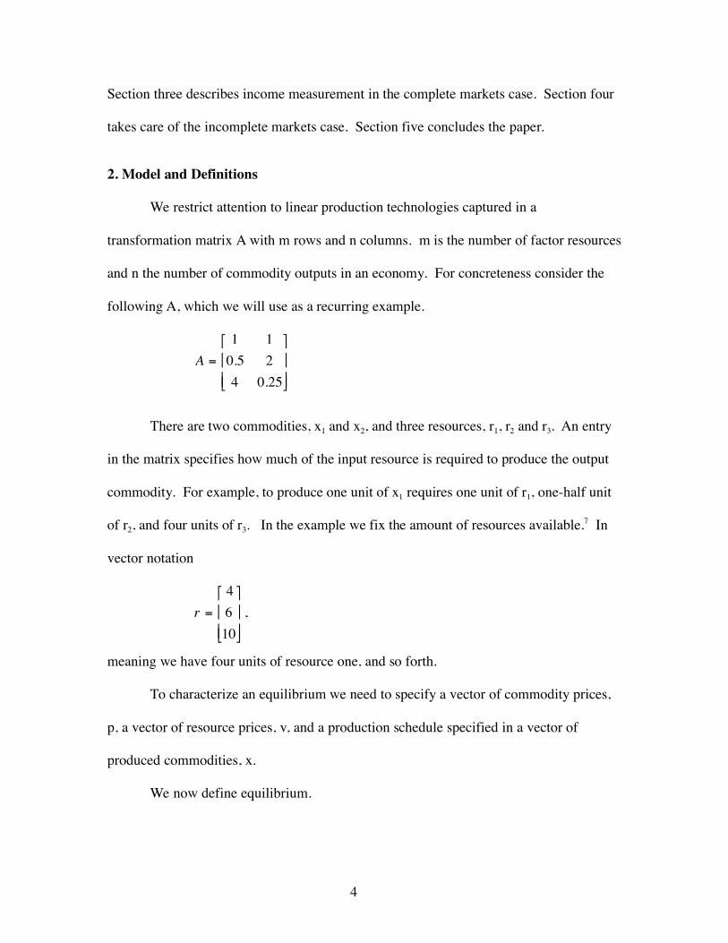
We restrict attention to linear production technologies captured in a

transformation matrix A with m rows and n columns. m is the number of factor resources

and n the number of commodity outputs in an economy. For concreteness consider the

following A, which we will use as a recurring example.

A =

1 1

0.5 2

4 0.25

!

"

#

#

$

%

&

&

There are two commodities, x1 and x2, and three resources, r1, r2 and r3. An entry

in the matrix specifies how much of the input resource is required to produce the output

commodity. For example, to produce one unit of x1 requires one unit of r1, one-half unit

of r2, and four units of r3. In the example we fix the amount of resources available.7 In

vector notation

r =

4

6

10

!

"

#

#

$

%

&

& ,

meaning we have four units of resource one, and so forth.

To characterize an equilibrium we need to specify a vector of commodity prices,

p, a vector of resource prices, v, and a production schedule specified in a vector of

produced commodities, x.

We now define equilibrium.

5

Definition: {p, v, x} is a competitive equilibrium if:

1. A.x ≤ r

These conditions simply state that the resources used by the commodities can not

exceed the resources available.

2. AT.v ≥ p

These conditions state that the cost of producing a unit of commodity should be no

less than the selling price of the commodity. This is just what we would ask of

competitive market prices. If the price of the commodity strictly exceeds the cost of

producing it, equilibrium forces would act to bid up the prices of the resources.

3. Prices in equilibrium are consistent with the demand functions. For exposition

purposes we will consider linear demand functions.

D.x = p, where D is a square matrix of dimension n.8

For our example D =!1 1

10 !1

"

# $ %

& ' .

4. Define Mi as the i-th row of a matrix M (so MTi is the i-th row of MT and the i-th

column of M). Then:

(i) If Aix < ri, then vi = 0.

(ii) If ATi .v > pi, then xi = 0.

Condition (i) states that if resource ri is not entirely used up, resource price vi is equal

to zero. That is, we do not require that all resources are used, but if they are not all

used, they are free. This is like sands in the Sahara. Condition (ii) states that if the

cost of commodity xi is greater than its price, none of the commodity is produced in

equilibrium. That is, we do not require that the costs to make a commodity are equal

7 We can expand the analysis to elastic supply of resources, but no further insights are

extracted, and the inelastic supply case is more streamlined.

8 Linear demand functions are not necessary for establishing relations among income, equilibrium prices, and efficiency. However, they are useful in calculating equilibria, and in our setting yield unique equilibrium prices.

6

to their benefit, but if they are not equal, it must be that the commodity is not

produced in equilibrium. This is like silk diapers.

5. Equilibrium prices and quantities are non-negative, with at least one price or quantity

positive. The purpose of the strictly positive condition is to eliminate the trivial and

uninteresting case where nothing is produced.

Notice that the definition of equilibrium says nothing about firms and their

objective functions. In particular, no assumption is made that firms maximize income (or

how income is measured).

The Concept of Income

At this point we appeal to the beautiful theory of linear programming in order to

demonstrate that the concept of income arises directly from our assumptions about

equilibrium conditions in the economy.

We first restate the equilibrium conditions.

A.x ≤ r AT.v ≥ p

x ≥ 0 v ≥ 0

where for resource i where for commodity i

if Aix < ri, vi = 0. if ATi .v > pi, xi = 0

The fact that the entries in A and the resource levels r are non-negative implies

that both sets of inequalities are feasible: we can always choose small enough xi's so that

A.x ≤ r and we can always choose large enough vi's so that AT.v ≥ p. This set of

conditions implies the following property of an equilibrium.

Observation 1: The quantity pT.x - vT. r is maximized by every competitive equilibrium.

7

Proof: Since v ≥ 0, premultiplying condition (1) by vT provides: vT.A.x ≤ vT. r. Since

x ≥ 0, premultiplying condition (2) by xT provides: xT.AT.v ≥ xT .p. Transposing both

sides yields: vT. A.x ≥ pT.x. Thus, vT. r ≥ vT.A.x ≥ pT.x, so pT.x - vT. r ≤ 0. In addition, we

know that vi Ai.x = vi ri and ATi .v.xi = pixi for the following reasons. First, if Ai.x = ri and

AT.v = pi the result follows immediately for any vi and xi. Second, if Ai.x < ri equilibrium

implies vi = 0 and if ATi .v > pi , equilibrium implies xi = 0, and again the result follows

immediately. Since this is true for all xi and vi, we have vT.A.x = vT. r and vT. A.x = pT.x,

we now have pT.x - vT. r = 0. And since we have previously proved pT.x - vT. r ≤ 0 in

equilibrium, pT.x - vT.r has attained its maximum when it is equal to zero.

The above observation implies equilibrium behavior is consistent with

maximization of a number, justifying the following definition of income. (The result is

produced without assuming anything about individual firm behavior.)

Definition: Income is the difference between the revenues generated by the commodities

produced in the economy, pT.x, and the cost of resources used by the economy in

production, vT. r.

The Concept of Efficiency

We now have developed the concept of income and defined it within our model.

The next step is to identify income's relation to productive efficiency, which we now

define.

Definition: A productive allocation is efficient if there does not exist any other

physically possible allocation which has more of at least one commodity and no less of

any commodity. Notationally, let x ≥ 0 satisfy A.x ≤ r. The commodity vector x is

8

efficient if there does not exist x' ≥ 0 such that A.x' ≤ r and xi' ≥ xi for all i, and xj' > xj for

some j.

The following observation states the aggregation feature of the income

calculation.

Observation 2: In equilibrium, income is maximized and economy-wide production is

efficient.

Proof. We have already shown in the proof of Observation 1 that income (as defined

above) is maximized in equilibrium. Consider the following two linear programs.

Program 1: Program 2:

maximize pT.x minimize vT. r x v

subject to: A.x ≤ r subject to: AT.v ≥ p

x ≥ 0 v ≥ 0

The two programs have the property that one is the dual of the other. We know an

equilibrium p, v, and x exists and satisfies the constraints of both programs, since it

satisfies (1), (2), and (5). Furthermore, as indicated in the proof of Observation 1,

equilibrium implies zero income, i.e., the objective functions are equal. Using the Duality

theorem of linear programming, it follows that in equilibrium x and v optimize both

programs. 9 Since x is optimal in Program 1 and commodity prices are non-negative, it

must be efficient. After all, if there existed another commodity vector, x', that is feasible

and which dominates x, then x would not have been a solution in the first place.

9

As Dorfman et al. (1987, p. 370) eloquently state, "hidden in every competitive

general equilibrium system is a maximum problem for value of output and a minimum

problem for factor returns." These are the primal and dual programs presented in the

proof of Proposition 1.10

We use the numerical example introduced previously to illustrate Observations 1

and 2.

Complete markets equilibrium

x1 = 0.9836 v1 = 0 p1 = 1.770

x2 = 2.754 v2 = 3.541 p2 = 7.082

v3 = 0

The objective function of each of the programs is 79,056 / 612 ≈ 21.25.

One can verify that the prices and quantities satisfy the equilibrium conditions (1)

through (5). In general, one can solve for an equilibrium by trying a set of prices and

solving for x and v using Programs 1 and 2, and then checking to see if they are

consistent with the demand functions. The procedure can be carried out systematically

by choosing a set of binding constraints in Program 1 and checking whether all the other

conditions are met. In this example, if one chose the first two constraints, one would

obtain 4/3 and 8/3 for the commodity quantities (both positive). The demand equations

9 The Duality Theorem of Linear Programming states, among other things, that if x and

v are feasible in the two programs, and if the objective functions are equal, then x and v are optimal in their respective programs. See Luenberger (1989, page 89).

10 The shadow price on the primal constraints are the resource prices, and the shadow price on the dual constraint is the commodity amount. If any of the constraints are non-binding, its corresponding shadow price is zero, just as one would desire in an equilibrium (property (4)). In fact, at the optimal solution the following is true:

10

would then dictate prices of 4/3 and 32/3 (both positive). But equilibrium condition (4)

would imply the price of the first resource is negative. Further investigation would reveal

that in this example no equilibrium is found when any two of the constraints in the first

program bind. One would then proceed to test cases where a single constraint is binding.

It turns out that the equilibrium is such that the second inequality alone is binding. The

equilibrium thus satisfies equations (a) through (e).

0.5 x1 + 2 x2 = 6 (a)

- x1 + x2 = p1 (b)

10 x1 - x2 = p2 (c)

0.5 v2 = p1 (d)

2 v2 = p2 (e)

The constraints (d) and (e) simply tell us the ratio of prices is 4, so we can solve

for the commodities by using (a) and (- x1 + x2)/(10x1 - x2) = 4. The solution is x1 =

60/61 ≈ 0.9836 and x2 = 168/61 ≈ 2.754. Next substitute into (b) and (c) to obtain the

commodity prices: p1 = 108/61 ≈ 1.770 and p2 = 432/61 ≈ 7.082.11 (One should verify

that all the inequalities are also satisfied.)

(Aix - ri)vi = 0 and (AT

i .v - pi)xi = 0. These are referred to as complementary slackness conditions.

11 One may avoid the trial-and-error approach by solving the following program (for a non-trivial solution). max pT.x - vT. r p, x, v

s.t. A.x ≤ r AT.v ≥ p D.x = p x ≥ 0 v ≥ 0 p ≥ 0

11

3. Complete Markets Accounting

The previous section laid sufficient groundwork to allow us to talk about

accounting issues. Specifically, the income number can be viewed as economy-wide

revenues (the objective function in the Program 1) minus economy-wide costs (the

objective function in Program 2). If all production in the economy is accomplished by

one firm, the income statement is as follows.

Income Statement: Complete markets - Economy Revenues:

x1 (0.9836)(1.77) = $ 1.74

x2 (2.754)(7.082) = 19.50

Expenses:

r1 0

r2 (.5)(.9836)(3.541)+ (2)(2.754)(3.541) = 21.24

r3 0

Income $ 0

Income calculation aggregates important economy-wide information about

equilibrium and efficiency into a scalar, the income number. In this paper we will

consider this aggregation activity as the accountant's job. We will discuss how difficult

the job is under two settings: (1) when there are two firms and trading is unrestricted, and

(2) when there are two firms but trading is restricted.

Two firms

12

It is useful to explore multiple firms (traders) so that we can compare complete

and incomplete markets.12 It turns out that the zero-income-property is not lost if

production is conducted by more than one firm. To continue with the numerical example,

suppose the two commodities are produced by two different firms. Firm A is endowed

with the technology to produce commodity 1; product 1 technology consists of the first

column of the A matrix. Similarly Firm B produces commodity 2. Furthermore, endow

the two firms with resources as follows.

Endowments

Endowments Firm A Firm B

resource 1 2 2

resource 2 3 3

resource 3 3 7

Notice that the total of each of the resources is the same as before. And, most

importantly, the equilibrium prices remain as in the previous section: 0.9836 units of

commodity 1 are produced (by Firm A) and 2.754 units of commodity 2 are produced (by

Firm B). The resource requirements for this production schedule are as follows.

12 Of course, in this setting there are no transactions costs, so it is hard to rationalize why

firms would exist (and even what they are). What we do need here is a set of trading entities.

13

Resource requirements -- Complete markets

Resource

requirements

Firm A Firm B Total

resource 1 0.984 2.754 3.738

resource 2 0.492 5.508 6.000

resource 3 3.934 0.689 4.623

Notice that Firm B requires more of resources 1 and 2 than are available from its

endowment. And Firm A has excess amounts of resource 1 and 2. The production plan

is still achievable because Firm A is permitted to trade some of its unused resources to B.

Also, Firm A requires more of resource 3 than is available from its endowment; its

production is accomplished by trading with Firm B. Trades of the resources will occur at

the following equilibrium prices: v1 = 0, v2 = 3.54, v3 = 0. Resource 2 is the only

resource with a positive price, as it is the only one whose supply is limited by the

equilibrium production schedule. The entire 6 units available is used in production.

As is well-known, income measurement and valuation are inextricably linked

(Beaver and Demski, 1995). Hence, calculation of individual firm income follows

directly once the resource prices are determined.

14

Income statements: Complete markets - Individual firms

Firm A Firm B

Revenues: (.9836)(1.77) = $ 1.74 (2.754)(7.08) = $ 19.50

Expenses:

resource 1 0 0

resource 2 (.4918)(3.541) = 1.74 (5.508)(3.541) = 19.50

resource 3 0 0

Income $ 0 $ 0

At equilibrium firm income remains at zero for all firms, as documented in the

following proposition.

Proposition 1: In a complete market setting each firm's income is zero in equilibrium and

is determined using market prices for commodities and resources.

Proof: From the complementary slackness condition, we know that if any commodity, say

xi, is produced, then ATi .v = pi. That is, the cost of resources used to produce the

commodity is equal to the revenue generated by the commodity. Each commodity yields

zero income in equilibrium, so irrespective of which commodities are produced by a firm,

its income is zero.

In complete markets, aggregate supply of each resource, not each firm's initial

endowment, is the determinant of equilibrium. That is, the p and v are the same as

though a single firm were undertaking all production. In the complete markets setting,

the economy operates as follows. Equilibrium forces determine p, v, and x. Individual

15

firms simply trade resources at resource price v (determined at the market level) to reach

equilibrium production.

Income measurement is instructive in that it is directly related to the efficiency of

the production plan. This is stated in the next Corollary.

Corollary 1: Given equilibrium prices, if each firm's income is zero the production

schedule is efficient.

Proof. Technology restrictions ensure that x satisfies the primal constraints; p and v

being equilibrium prices ensure that the dual program is optimized. Each firm's income

being zero implies economy-wide income is zero, which implies pT.x = vT. r. The Duality

theorem then implies that x optimizes Program 1, i.e., x is efficient.

Even at the individual firm level, the income number retains its ability to

aggregate information about the economy. The accountant's job is still not a difficult

one, as income measurement follows directly from the observation of resource and

commodity prices. The prices are easily determined as transactions occur at that price.

"Mark-to-market" is a viable and effective valuation rule. However, the situation

becomes more complex when markets are incomplete. The next section explores this

issue.

4. Incomplete Market Accounting

In this section we confront accounting in incomplete markets. We model market

incompleteness by restricting the trading opportunities. In particular, for the numerical

example we prohibit trading in resource 3. Now each firm must design its production

schedule with its use of resource 3 restricted to its initial endowments.

16

The way we capture the additional restriction is to reformulate the transformation

matrix, A. Additional rows are added, and the resources are labeled r1, r2, r3A, and r3B.

Given the restriction on trading in resource 3, we treat it differently for each of the firms,

despite the resource being physically identical. The distinction between r3A and r3B is not

the physical composition but rather the market restriction on trading. The linear

formulation proves convenient since all definitions we have provided earlier (and the

technique suggested for computing the equilibrium) remain valid except that the

reformulated A matrix is used.

A =

1 1

.5 2

4 0

0 .25

!

"

#

#

#

$

%

&

&

&

r =

4

6

3

7

!

"

#

#

#

$

%

&

&

&

The equilibrium in the incomplete market setting is as follows. 13

Incomplete markets equilibrium

x1 = 0.7500 p1 = 2.063 v1 = 0

x2 = 2.813 p2 = 4.688 v2 = 2.344

v3A = 0.2227

v3B = 0

The objective function for each of the programs is 14.73.

13 The following equalities are satisfied by an equilibrium.

0.5 x1 + 2x2 = 6 4 x1 = 3 p1 = - x1 + x2 p2 = 10x1 - x2 0.5 v2 + 4v3A = p1 2 v2 = p2

17

Resource requirements -- Incomplete markets

Resource

requirements

Firm A Firm B Total

resource 1 0.75 2.813 3.563

resource 2 0.375 5.625 6.000

resource 3 3.000 0.703 3.703

Income measurement is now problematic since there has been no transaction

involving resource 3, hence, a market price is unavailable. Nonetheless, when the

individual shadow prices v3A and v3B are used in the income calculation, the illuminating

property of income is preserved in the sense that zero income accompanies equilibrium.

The use of shadow prices in income calculation parallels that in Scapens (1978) and

Beaver and Demski (1995), who refer to them as "personal prices." 14 For the example

the income statements follow.

Income statements: Incomplete markets

Firm A Firm B

Revenues: (.75)(2.063) = $ 1.55 (2.813)(4.688) = $ 13.18

Expenses:

resource 1 0 0

resource 2 (.375)(2.344) = 0.88 (5.625)(2.344) = 13.18

resource 3 (3)(.2227) 0.67 0

Income $ 0.00 $ 0.00

14 Personal prices are used in the economics literature on efficiency in incomplete

markets, e.g., Geanakopolos, Magill, Quinzii, and Dreze (1990).

18

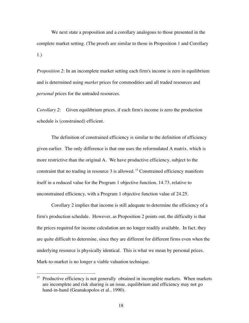
We next state a proposition and a corollary analogous to those presented in the

complete market setting. (The proofs are similar to those in Proposition 1 and Corollary

1.)

Proposition 2: In an incomplete market setting each firm's income is zero in equilibrium

and is determined using market prices for commodities and all traded resources and

personal prices for the untraded resources.

Corollary 2: Given equilibrium prices, if each firm's income is zero the production

schedule is (constrained) efficient.

The definition of constrained efficiency is similar to the definition of efficiency

given earlier. The only difference is that one uses the reformulated A matrix, which is

more restrictive than the original A. We have productive efficiency, subject to the

constraint that no trading in resource 3 is allowed. 15 Constrained efficiency manifests

itself in a reduced value for the Program 1 objective function, 14.73, relative to

unconstrained efficiency, with a Program 1 objective function value of 24.25.

Corollary 2 implies that income is still adequate to determine the efficiency of a

firm's production schedule. However, as Proposition 2 points out, the difficulty is that

the prices required for income calculation are no longer readily available. In fact, they

are quite difficult to determine, since they are different for different firms even when the

underlying resource is physically identical. This is what we mean by personal prices.

Mark-to-market is no longer a viable valuation technique.

15 Productive efficiency is not generally obtained in incomplete markets. When markets

are incomplete and risk sharing is an issue, equilibrium and efficiency may not go hand-in-hand (Geanakopolos et al., 1990).

19

To estimate the personal prices of untraded resources requires examining the

entire economy including the allocations and prices of the traded assets. Notice that in

the numerical example the prices of all the commodities changed, as well as the price of

resource 2, even though there were no restrictions placed on trading in those markets.

This implies that the valuation problem can not be decomposed into a preliminary

analysis of unrestricted markets concatenated with an analysis of the restricted markets.

The entire economy must be considered simultaneously.

5. Conclusion

This paper demonstrates that aggregating information in the form of an income

number is illuminating about the state of the economy. Income, by itself, reflects

whether or not the economy is in equilibrium, and using a standard result in welfare

economics, whether or not the allocation of resources is productively efficient. These

results hold even when the market structure is not complete, that is, when some assets can

not be traded.

However, what is different across complete and incomplete markets is the ease

with which such a number can be computed. The accountant's job as an income

calculator is significantly more difficult when markets are incomplete, as there are no

market prices on which to rely. Instead the accountant must rely on personal prices. The

estimation of personal prices requires a deep understanding of the equilibrium forces at

work in the economy.

20

References

BEAVER, W., AND J. DEMSKI. "Income Measurement and Valuation." Working paper,

University of Florida 1990.

CHAMBERS, R. Accounting, Evaluation and Economic Behavior. Prentice Hall, 1966.

DEBREU, G. Theory of Value. New Haven, CT: Yale University Press, 1959.

DORFMAN, R., P. SAMUELSON, AND R. SOLOW. Linear Programming and Economic

Analysis. New York: Dover Publications, 1987.

EDWARDS, E., AND P. BELL. The Theory and Measurement of Business Income.

University of California Press, 1961.

GEANAKOPLOS, J., M. MAGILL, M. QUINZII AND J. DREZE. "Generic Inefficiency of Stock

Market Equilibrium when Markets are Incomplete." Journal of Mathematical

Economics 19 (1990).

LUENBERGER, D. Linear and Nonlinear Programming. Reading, MA: Addison-Wesley

Publishing Company, 1989.

PATON, W. Accounting Theory. Accounting Studies Press, Ltd., 1922.

SCAPENS, R. "A Neoclassical Measure of Profit." The Accounting Review 53 (April

1978).

STERLING, R. Theory of the Measurement of Enterprise Income. University of Kansas

Press, 1970.