INC ALBUQUERQUE NM PARALLEL-PLATE TRANSMISSION LINE ...
172
/AOAO86 814 DIKEWOOD INDUSTRIES INC ALBUQUERQUE NM F/6 20/14 PARALLEL-PLATE TRANSMISSION LINE TYPE OF EMP SIMULATORS: SYSTEM--ETC (U) MAY 80 D V GIRI. T K LIU, F M TESCHE F29601-78-C-0045 NCLASSIFIED DC-FR1299-4 AFWL-TR-79-139 NL IllAllllllll000001 lllllllllnmll Smmmhhhmmhhhhla
Transcript of INC ALBUQUERQUE NM PARALLEL-PLATE TRANSMISSION LINE ...

/AOAO86 814 DIKEWOOD INDUSTRIES INC ALBUQUERQUE NM F/6 20/14PARALLEL-PLATE TRANSMISSION LINE TYPE OF EMP SIMULATORS: SYSTEM--ETC (U)MAY 80 D V GIRI. T K LIU, F M TESCHE F29601-78-C-0045
NCLASSIFIED DC-FR1299-4 AFWL-TR-79-139 NL
IllAllllllll000001lllllllllnmll
Smmmhhhmmhhhhla

AFWL-TR-79-1 39 L N LAFWL-TR-
41!14PARALLEL-PLATE TRANSMISSION LINE TYPE OF.__4u 000 EMP SIMULATORS: SYSTEMATIC REVIEW AND
00 RECOMMENDATIONS
D. V.Giriet al.
00Dikewood industries, Inc1009 Bradbury Dr., SEAlbuquerque, NM 87106
May 1980
ELECTE fFinal Report190j
Approved for public release; distribution unlimited.
4V
AIR FORCE WEAPONS LABORATORYAir Force Systems Command
Kirtland Air Force Base, NM 87117
80 6 10 008

AFWL-TR-71 39
This final report was prepared by Dikewood Industries, Inc., Albuquerque,New Mexico, under Contract F29601-78-C-0045, Job Order 37630274 with the AirForce Weapons Laboratory, Kirtland Air Force Base, New Mexico. Captain HowardG. Hudson (NTYE) was the Laboratory Project Officer-in-Charge.
When US Government drawings, specifications, or other data are used for anypurpose other than a definitely related Government procurement operation, theGovernment thereby incurs no responsibility nor any obligation whatsoever, andthe fact that the Government may have formulated, furnished, or in any waysupplied the said drawings, specifications, or other data, is not to be regardedby implication or otherwise, as in any manner licensing the holder or any otherperson or corporation, or conveying any rights or permission to manufacture, use,or sell any patented invention that may in any way be related thereto.
This report has been authored by a contractor of the United StatesGovernment. The United States Government retains a nonexclusive, royalty-freelicense to publish or reproduce the material contained herein, or allow othersto do so, for the United States Government purposes.
This report has been reviewed by the Public Affairs Office and is releasableto the National Technical Information Service (NTIS). At NTIS, it will beavailable to the general public, including foreign nations.
This technical report has been reviewed and is approved for publication.
HOWARD G. HUDSONCaptain, USAFProject Officer
FOR THE DIRECTOR
6).L[J PHILP AS LLO, PhD THOMAS W. CIAMBRONE%hief, Electromagnetics Branch Colonel, USAF
Chief, Applied Physics Division
D
DO NOT RETURN THIS COPY. RETAIN OR DESTROY.

UNCLASSIFIEDSECURITY CLASSIFICATION OF TWIS PAGE ("R 0400 4Rutm~d) _________________
REPORT DOCUMIENTATIQN PAGE BFR OPEIGFRT. R9PORT NUM@9U 2.43V ACCESSION No. REmc! I9NT CATALOG NUMBER
AFWL-TR-79-1 39 ~ ,%,26 _____________
4 6. TITLE (8040 StuMid.) S. Type OF REPORT a PERIOD COVERED
PARALLEL-PLATE TRANSMISSION LINE TYPE OF EMP Final ReportSIM4ULATORS: SYSTEMATIC REVIEW AND 4. PERFORMING Ono. IeORT NDMERRECOMMENDATIONS DC-FR-i1299-4
7. AUNOR() 8.CONTRACT OR GRANT NUNS91(a)
0. V. Girl R. W. P. King*T. K. Liu F29601 -78-C-0045F. M. Tesche*
-t EFRIGORGANIZATION NAME AND ACRMS 10. PROGRAM ELEMCENT. PROJECT, TASKPERORIN 1AREA & WORK UN'IT NUMBERS
Dikewood Industries, Inc.T1009 Bradbury Drive, S.E. 64711 Ff37630274Al buquerque, NM 87106 _______________
1I. CONTROL.LING OFFICE N4AME AND ADORCSS Ia. REPORT DATE
Air Force Weapons Laboratory (NTYE) ~ ~ may 198013 UMBER OF P AG ES
Kirtland Air Force Base, NM 87117 16614. MONITORING AGENCY NAME A ACOORESSi'dI,ifst from Controlling Office) I5. SECURITY CL.ASS. (of this report)
Unclassi fiedjIBe. CCI ASM PI CATION/ DOWNGRADING
I SCM EDULE1
Is. DISTRIBUTION STATEMENT (01 this XOP041)
Approved for public release; distribution unlimited.
IT. DISTRIBUTION STATEMENT (of the abstrait f mtrd ill Stock 20. It ditt~ a 9 om ROpeatI 16. SUPPLECMENTARY NOTESSubcontractor: *LuTech, Inc., 5301 Central Ave., N.E., Albuquerque, NM 87108.
**Harvard University
It. KEY *ORMo (ConuIwan ri evuerse Old* It n..oesermad idstifif6 b lock RVNIMho)
Conical Transmission LinesE14P Pul so GeneratorsEMP SimulatorsParallel-Plate Transmission Lines
20. ABSTRACT (CoiMu. OR 00100 , 01400 it MwooPW Sod Idet~fF' 1W Uslt inf
This report presents various aspects of the two-parallel-plate transmissionline type of EM4P simulator. Much of the work is the result of researchefforts conducted during the last two decades at the Air Force WeaponsLaboratory, and in industriesluniversities as well. The principal featuresof individual simulator components are discussed. The report also emphasizesthat it is imperative to hybridize our understanding of individual components
DI ,0731473 UNCLASSIFPIEDSECURITY CI.ASSIPICATION 00 Tw414 PAGE (Shan Do@m Zered

UNCLASSIFIEDSICCURITY CLASSIFICATION OF THIS PAOU(UIIo Data Etn*.d)
20. ABSTRACT
so that we can draw meaningful conclusions of simulator performance as awhole.
II
S
UNCLASSIFIEDSICUMITY CLASIOPICATION OF THIS PA@WS l'U D41 hmm

SUMMARY
In this report, we have attempted to summarize the
various aspects of the two-parallel-plate transmission line
type of EMP simulator. Much of the work, briefly reported
here, is the result of research efforts during the last twodecades at the Air Force Weapons Laboratory, and in industry/universities as well. It was considered useful to bring
under one cover, the principal features of individual
simulator components. In addition, our understanding ofthe performance and problems associated with the individualsimulator components needs to be combined in such a manner
that one can draw conclusions about the simulator performance
as a whole.
To appreciate the magnitude of work that has beenaccomplished, the reader is encouraged to consult reference
[S.11, which lists about 50 references from the EMP Notesand Memo series. However, one rapidly recognizes that the
analytical/numerical efforts address relatively simplerdesign aspects. But in reality, practical considerationsresulting in engineering compromises make the problem much
harder. With these considerations in mind, we have in-
cluded a section on the simulator as a whole which lists
some of the problem areas while pointing out their principal
features.
The approach taken in this report is to brieflysummarize in various sections, the available data/resultswith regard to the constitutive elements of the simulator
(e.g., pulser, conical and cylindrical transmission line,etc.). However, in interpreting these results in the con-text of the simulator proper, one has to keep in mind the
implications of the approximations made in the analysis
procedures. An example of these is the available results!.

on the propagating modes (TE, TM and TEM) in two-parallel-
plate transmission lines. Being an open-structure, suchmodal representations are valid only in and very near the
parallel plate region, while they grow unbounded as onemoves away in the transverse plane. In addition, for
transmission line treatment, the length of the line should
at least be several times larger than separation, a con-
dition which is not satisfied in the simulator facilities.
In spite of such approximations, the modal representation
of the working volume fields appears to be the best
available framework for interpreting and comparing themeasured fields with calculations.
We have condensed the available information
on two types of pulsers (Van de Graaff and Marx) with
the view of providing a working knowledge of theseEMP pulsers especially to the readers concerned with
electromagnetic aspects. This is followed bydiscussions which deal respectively with the conical
and parallel-plate transmission lines. The TEM
quantities (characteristic impedance and field distribu-
tion) in two-conical-plate transmission lines are wellknown (3.2 and 3.33, while no work has been attempted on
the evaluation of non-TEM modes in the conical transmissionlines. However, in the central parallel-plate region,
detailed information is availabe on the TEM, TE01 and
TMOn modes. A knowledge of the properties of TEM and non-TEM modes in parallel plate transmission lines is extremely
useful in understanding and interpreting the measured
working volume fields.
It is impractical and prohibitively expensive tobuild bounded wave simulators long enough so that the
reflections from unterminated line will not arrive back in
2

the working volume to contaminate the object response.This creates the need for a "proper" termination at the
far end of the simulator. These issues are then addressed
while summarizing the available theoretical and experi-
mental studies. Furthermore, a laboratory model boundedwave simulator has been in existence since 1976 at
Harvard University for controlled experimental studies,e.g., detailed field maps at specific frequencies,terminator development, simulator/object interaction, etc.
Professor R.W.P. King of Harvard University (one of theauthors of this report) has included a review of the
experimental work.The topic of simulator/object interaction has
received some attention in the past and is reviewed.Careful experimental studies in this area are considered
highly desirable.
As was pointed out repeatedly in this report, inthe final analysis, we need to draw meaningful conclusionsabout the properties and performance of the simulator asa single electromagnetic structure. With such considera-
tions in mind, we have listed several problem areas thatmerit attention in the future. Needless to say, based onvalue judgments, there are avenues open for cost effectivelyadvancing this technology. The report is concluded with a
list of references.
ACCESSION forNTIS Wite SectionDDC Buff Section 3UNANNOUNCED 0JUSTIICATIGN
BY
DSTmBUTIW/ AML MLAI W01SDist. AVAIL and/a '
3
m _ .+ .-... L ' -.. ,.. z + __

PREFACE
In compiling a document of this nature, we are
deeply indebted to many individuals whose published
work has been freely used. Drs. K.S.H. Lee and C.E.
Baum have provided constant support. Special thanks
are also due to Ms. Kathy Magann for her painstaking
assistance during the preparation of this report.
4

CONTENTS
Section Page
I INTRODUCTION 9
II PULSE GENERATORS 13
II.1 Introduction 13
11.2 Van de Graaf Pulse Generator 15a) Energy storage 16b) Voltage generator 19c) Output switch 20d) Output section 20e) Pulser equivalent circuit 20
11.3 Marx Generator 22a) Equivalent circuit 25
III CONICAL-PLATE TRANSMISSION LINES 31
I11.1 Impedance 33
111.2 Fields 39
IV PARALLEL-PLATE TRANSMISSION LINES 45
IV.I Introduction 45
IV.2 Infinitely Wide and InfinitelyLong Parallel Plates 47
IV.3 Finitely Wide and InfinitelyLong Parallel Plates 50
a) TEM Mode 52b) Non-TEM Modes 56
IV.4 Source Excitation 67
IV.5 Experimental Results 70
IV.6 Modal Representation ofMeasured Fields 72
1 __ 5

V TERMINATIONS FOR THE SIMULATORS 80
V.1 Introduction 80
V.2 Values of the Terminating Elements 81
V.3 Idealized Analyses 83
V.4 Practical Considerations 87
V.5 Experimental Evaluation and Optimization 92
V.6 Example 93
V.7 Recommendations 96
VI A REVIEW OF AVAILABLE EXPERIMENTAL WORK 98
VI.l Introduction 98
VI.2 The Harvard EMP Simulator 99
VI.3 Preliminary Measurements 103
VI.4 Introductory Description of the Fieldin the Parallel-Plate Region 108
VI.5 The Field in the Parallel-Plate Section;TEM and TM Modes 112
VI.6 The Measured Field in the Working Volume;b = 2.25X =108 cm, f = 626.5 MHz 118
VI.7 The Measured Field in the Working Volume;b = 0.66X = 75 cm, f = 264 MHz 127
VI.8 The Transverse Variation of the ElectricField; TE Modes 127
VI.9 The Actual Electromagnetic Field in theSimulator as an Approximation of aPlane Wave 129
VI.10 Possible Methods to Improve the Field inthe Simulator as an Approximation of aTraveling Plane Wave 133
VII SIMULATOR/OBJECT INTERACTION 137
VII.1 Introduction 137
VII.2 SEM Representation 139
VII.3 Fields near the Test Object 148
6

VIII SIMULATOR AS A WHOLE 154VIII.1 Problems List 155
VIII.2 Brief Discussion of SalientFeatures of Listed Problems 156
REFERENCES 160
7/8

I INTRODUCTION
Bounded wave EMP simulators, of the two-parallel-
plate transmission line type, are complex electromagnetic
structures that should be analyzed in their entirety. In
view of the difficulties in analyzing a structure like
ALECS (one plate above a ground plane; vertically polarized
electric field) or ATLAS I (also called TRESTLE with two
parallel plates; horizontally polarized electric field),
various analytical/numerical efforts in the past have
addressed relatively simpler structures which are idealized
versions of individual simulator components. An example of
this is the short (length not too large compared to
separation), central parallel plate region which is treated
as a finitely wide, two-parallel-plate transmission line.
It is essential, however, to put together our understanding
of individual components in a manner that helps us in
evaluating the overall performance of the simulator.
We have attempted in the initial sections (II thru
V) of this report, to briefly summarize the principal results
of the treatments of individual simulator components.
Figure 1.1 shows a schematic of a parallel plate transmission
line type of EMP simulator comprised (from right to left)
of a pulser, wave launcher, central parallel plate region,
wave receptor and a terminator. The planning and design
of the facility would naturally have started from the
central parallel plate region and evolved toward the pulser
on the input side, and the terminator on the output side.
However, this report is organized in a different manner
from the way the simulator thinking has evolved. After this
introductory section, we have essentially followed the
simulator components starting from the pulser in Section II
and following the direction of propagation of the wave, i.e.,
9!

41y44-
5-4
00
to- 0
E
CL
0
V)J 4-
,'U
V4-
0
0'-0
E-4
10

conical transmission line (wave launcher and receptor
sections), parallel plate transmission line and the terminator.
Specifically, in Section II, we have condensed the
available data on the Van de Graaff pulse generator (used,
for instance, in the ARES facility) and the Marx pulse
generator employed in the ATLAS I facility. This section
furnishes a working knowledge'of these two types of pulse
generators for readers interested in electromagnetic aspects
of the facilities (ALECS, ARES, ATLAS I and II). Section
III discusses the TEM characteristics of the conical trans-
mission line. In this regard, one may note that no calcula-
tions are available on the properties of non-TEM modes in
conical lines. On the other hand, detailed calculations of
the TEM and non-TEM (TE and TM) modes in parallel plate trans-
mission lines are available in the literature and summarized
in Section IV. In Section V, we have reviewed the subject of
terminators for this class of EMP simulators. Several theoreti-
cal treatments of perpendicular and sloped terminating sections
are available for the case of infinitely wide plates. More
importantly, an extensive experimental evaluation of the
terminator was conducted (circa 1974) in the ALECS facility,
and the results of this study are summarized here along with
recommendations for future designs.
With the view of being able to perform controlled
experiments, a laboratory model parallel plate EMP simulator
has been in existence since 1976 at Harvard University. Some
of the experiments that have been, and are being performed with
this laboratory model simulator are:
a) careful and complete field mapping in the
parallel plate region,
b) terminator development,
11

c) suppression of non-TEM modes by taking
advantage of the known TEM and non-TEM
field distributions,
d) measurement of representative object responses,
e) simulator/object interaction studies,
f) evaluation of some of the trestle effects, e.g.,
the platform,
etc.
In Section VI, Professor R.W.P. King (one of the authors of
this report) has included a review of the presently available
experimental results.
With regard to the subject of simulator/object
interaction, the available theoretical work is reviewed in
Section VII. One of the approaches in the past has been to
use SEM representation, i.e., to trace or follow the changes
in SEM parameters as one varies the relative simulator/object
geometry. There appears to be no single physical parameter
which can effectively quantify all of the simulator/object
interaction effects. Careful and extensive experimental
investigation of these effects on the laboratory model
simulator is highly recommended as a future effort.
In Section VIII entitled "Simulator as a Whole"we have addressed some of the questions deserving further
study to help analysts in evaluating the overall character-
istics of this class of bounded wave simulators. The report
is concluded with a list of references.
12

II PULSE GENERATORS
II.1 Introduction
From an electromagnetic point of view, considerably
more is known about the simulation proper than the associated
pulse power 12.1]. Generally speaking, the pulsers for EMP
simulators depend on the basic properties of the electrical
discharge process for the design and fabrication of fast
switches and other pulser components. This indicates a
need for seeking answers to basic questions concerning the
properties of materials used in various pulser components.
In addition, from a macroscopic viewpoint, one might think
of the pulser in its entirety as a wave generator responsible
for producing, transporting across its own various stages,
and launching on to the simulator, a travelling wave with
a reasonably planar wavefront, by the time it reaches the
working volume. Put differently, it is not adequate to
think of the pulser as a high voltage (typically up to
5 MV), fast rising (t10_90 of < 20 ns) pulse generator. It
is imperative to consider and, in some sense, optimize the
properties of wave transport across various stages/inter-
faces within the pulser via the considerations of spatial,
temporal and spectral content of the waveform. An example
of such considerations lies in assuring proper wave
matching (both in impedance and field) in and between
various Marx pulser elements, namely the odtput switch and
its interface with the central Marx column and peaker
assembly. In the present configuration, shown in Figure
2.1 the monocone output switch has an impedance of 88Q,
as opposed to simulator or load impedance of ~-150Q. The
input impedance of the simulator, which acts as a load to
the pulse generator, is largely dominated by the character-
istic impedance of the principal TEM mode owing to the fact
13

00
0 0
g -U .'
1* '
N 1.4
0:
01

that the non-TEM modes do not propagate near both ends of
the simulator. Hence, it is desirable to maintain a con-
stant impedance zTE of the simulator across the
various pulser elements, in addition to minimizing field
discontinuities across junctions and interfaces. Presently,
work is just being commenced by LuTech personnel under a
separate effort, that specifically addresses such wave
matching questions. The approach being followed is:
(1) to investigate ways of increasing the impedance of the
output monocone switch from its present value of 880, (2)
to optimize the number and location of peaker arms and
(3) to understand the properties of wave transport on the
Marx column by modeling the Marx-peaker assembly by coupled
transmission lines. The results of this study are expected
to yield design curves and tables useful in future pulser
design and possibly in suggesting modification to existing
pulser designs.
The two types of pulse generators that have been
used for the bounded wave simulators are Van de Graaff (ARES
facility) and Marx (ATLAS I facility). In the remainder of
this section, we shall briefly summarize the principal
features of these two types of pulse generators [2.2, 2.3
and 2.4].
11.2 Van de Graaff Pulse Generator
Basically this ARES pulser is a dc charged system
employing a coaxial gas line capacitance, relying on proven
Van de Graaff and flash X-ray machine technology [2.2].
The pulse generator is a combination of the individual
elements, viz., energy store, voltage generator, output
switch and the output section. The pulser assembly is
15
.I.. ...__. . : ,II _ _ _ _ _ _' Illll I7

schematically sketched in Figure 2.2, showing the various
elements. At the output end, the transition departs fromcoaxial geometry and fans into a stripline, with anappropriate characteristic impedance controlled by spacing
to width ratio. The edges of the stripline are curved toprevent flashover. The insulating medium also transitions
from oil -- SF6 at 1 atmospheric pressure -- air. This
coaxial gas line design is a low impedance (15 to 20n)source wherein the energy is stored and discharged directlyinto the ARES input conic section. The idealized staircasewaveform, by discharging a l5f source into ARES
(Zc : 125n), approximates the desired pulse shape as
shown in Figure 2.3.
The electrical and mechanical characteristics of
the main pulser components are reproduced below fromReference (2.2] compiled by Ion Physics Corporation
personnel.
a) Energy storage
This is accomplished in a simple coaxial structure
(- 159 characteristic Z store impedance) formed by thecylindrical pressure vessel wall and an inner cylindrical
assembly supported by and directly coupled to the Van de
Graaff voltage generator as illustrated in Figure 2.2. Thecharacteristics of this coaxial line storage are as follows:
Effective Outer Diameter Nominal 3.35 m
Effective Inner Diameter Nominal 2.59 m
Characteristic Impedance Nominal 15.5 n
Physical Length Nominal 8.53 m
Electrical Length Nominal 54 x 10-9 s(Double Transit)Total Pressure, $300 psigDielectric Gas Mixture
16
7j-

IC
r4 I
us 4-4
(n 0
17 .

0i
0a 4
0.0
0e 0
07 LM
3 1 N 0C
'~4~ U~ -4m Ec
4J M gVQ C
.. 10 -r 4)00-r
00
41
-F n 'ar - 4)
8..I *w4 )4F-4 -4 0
0 0.inno
C~4
00
30V110A 38vH3
30VJ110A LfldiLfo
S ~ ~18 ---

Partial Pressures- 80% N : 20% CO2Optional 95% N2 : 5% SF 6Storage Charge Voltage 5.06 MV (Nominal)at 4.5 MV Load
Electrical, Radial Stress 15 MV/mat 5.06 MV Charge
Predicted Maximum =19 MV/mRadial Stress
Total Capacitance of =2000 pFStore
Energy Stored at 5 MV 25 kJCharge
b) Voltage generator
It is evident that the voltage generator must, at
a minimum, charge the store capacitance of 2000 pF to a
voltage of 5 MV in a satisfactory operational time. The
voltage generator has the following characteristics:
Generation Method Van de Graaff GeneratorSingle Belt (Option forTwo)
Polarity Positive or Negative
Belt Width 21.0 Inches (Effective=10 Inches)
Belt Speed 530 in/s
Maximum Belt Charge =10 - 7 C/square inch
Maximum Charge Rate 550 pA
Charge Rate for a 30-s 330 pACharge TimeInsulating Column Length 7 ft
Maximum Stress per Unit 1 MV/ftLength
Working Stress at 5 MV 0.71 MV/ft
The generator is both capacitively and resistively
voltage graded. The resistors which are 1% components are
also used to monitor the generator voltage as a check on the
generating voltmeter.
19
j

c) Output switch
It is an important feature of dc charged generators
that only a single switch is needed between the energy store
and the operating load. In the present configuration, this
switch is formed by the end of the energy storage terminal
and the output bushing cap. The switch gap length may be
continuously varied from 1.5 to 15 inches. The switching is
accomplished by a system of trigger pulse generators and
amplifiers on light signal command from a light source
operating external to the machine.
d) Output section
This is comprised of the output bushing assembly
(capacitively graded structure constructed of annular insula-
tors) and the output 125Q transmission line that provides
the necessary interface between the pressurized gas medium
to oil. Also, to facilitate controlled reduction in fall
time to 100 ns, an energy diverter is fitted into the oil
line, at the leading edge of the output transition.
e) Pulser equivalent circuit
A simple circuit model for this pulse generator,
neglecting stray reactances, is shown in Figure 2.4 where
C1 = capacitance of Van de Graaff column
Zo = coaxial gas line characteristic impedance
T S one way transit time of the gas line
c speed of light in the gas line medium
Co output bushing capacitance
Lo 0 switch inductance
RL = characteristic impedance of output strip
transmission line.
Circuit analysis leads to the voltage at
0-20
j|~m|A

-4
'444-4
0
1 0 044
0 Vn4-
-4 0
4.3,1
4I
C4
4
C.)
'21
-I C.)

(S) = L1 + O + LC s2] 11( Cs (2.1)L L 0 0. + L C0/s
where V1 (s) and Il(s) are respectively voltage and current
spectrum at the location x = xI = cT, which is the output
end of the gas line. From equation (2.1), it is also possible
to compute the voltage spectrum at the load VL (s) and con-
vince oneself that it approximates the desired double
exponential pulse. However, there is one limitation, that is,2if one computes the power spectrum (proportional of !VL(S) ),
there are nulls in energy delivered to the simulator at
specific frequencies.
II.3 Marx Generator
A schematic of the Marx-type of pulse generator, which
was configured into the Pulser Testing Fixture (PTF) for
evaluation purposes, is shown in Figure 2.5. It bascially is
comprised of an output bicone switch (can be replaced by a
monocone as in Figure 2.1), the peaking capacitor arms and the
Marx column along with the interconnections. The geometrical
and mechanical details of all the components along with the
electrical characterization of the key elements are available
in Reference [2.3], which is a collection of 18 technical
memoranda on the subject by Maxwell Laboratories, Inc.
In order to develop an equivalent circuit model for
the Marx pulser, it is required to determine the pulser
parameters that are geometry dependent as well as internal
parameters. The notational details for a typical output wave-
form are shown in Figure 2.6, where V and V arec prespectively the charge and peak voltage amplitudes. The
ratio (V p/VC ) is a measure of pulser efficiency. Some of
the typical problems with the pulser output waveforms, e.g.,
22

~03
U) C.
u4.
Cc0
41)
04
<0
LUU
.)
'4
.4
4 -P
0
C -4
oLA
10
U) Li
<w<
I.-40.0 0.
OCJ 4
23

vp P
(notch
prepulse
t
time
Fiqure 2.6. Pulser output waveform
24

prepulse, notch after the peak, are symbolically shown in this
figure. The prepulse is the part of the output waveform that
occurs prior to closing of the output (bicone or monocone)
switch at a time t = tO (say).
a) Equivalent Circuit:
The equivalent circuit models for a pulser unit cell,
i.e., one stage of Marx and a single peaker, are shown in
Figures 2.7a and 2.7b, respectively. They comprisent mt ext extinternal (LM n t Lp ) and external (L x , Lp ) induct-
ances and, likewise, internal (CM, Cint) and externalCext _ext.(M , p ) capacitances. The charging resistor for each
Marx stage is denoted by Rcharge* The Marx stages and
peakers also have capacitances to ground (CMg and CP9
in addition to mutual or coupling capacitances CMP. All
of these are either known or calcuable quantities. The
overall equivalent circuit consists of several Marx stages
combined in series, with peaker circuits in parallel. This
Marx-peaker combination, through an output switch, delivers
energy to the simulator as schematically shown in Figure 2.8.
With a knowledge of the equivalent circuit elements,one can compute the pulser output waveform via transmissionline theory and circuit analysis, for comparison with experi-
mental measurements on such features as prepulse, rise time,
peak amplitude, etc. From reviewing the available data,
improvements in pulser performance appear possible, by
initially analyzing the pulser geometry as a boundary value
problem in an attempt to get a clear understanding of the
properties of wave transport. Some of the relevant issues
here are the optimization of the number and relative orienta-
tion of peakers, computation of pulser output waveforms in
frequency and time domain, etc.
25

R charge
C
L Mp
Mp .
-S L
p C LR
p p p
CCM]I-%
L exoutpui t s ih
0'0
peaker
X to* simulator
L
Figure 2.8. Schematic overall equivalent circuit
26

A similar Marx pulser system, illustrated in Figure
2.9, is being used in the ATHAMAS II or the VPD II facility.
In this configuration, the peaking capacitor is physically
located in and approximately co-planar with the ground plane.
The water dielectric peaking capacitor feeds a uniform 60a
monocone by way of a self closing, pressurized SF6 gas output
switch. The monocone itself is a continuous structure con-
tained within a dielectric enclosure filled with Freon 12
gas to electrically insulate the conducting surfaces until
the electric fields associated with the highest operating
voltage have decreased to a low enough value. A summary of
the VPD II pulse generator parameters, both physical and
electrical, is given below [2.4].
Marx
1. Erected series capacity 3.50 nF
2. Number of stages 65
3. Output voltage (open circuit nVo) 6.5 MV maximum
4. Stage capacity 228 nF
5. dc charge voltage 100 kV maximum
6. Stray series inductance - 6.5 pH
7. Series resistance(stray = 3.5Q, lumped 2.5Q) 6a
8. Insultation oil
9. Marx switches
. gas type N2/SF6
• pressure 0 to 30 psig
10. Marx output voltage range 3:1
11. Marx erection jitter - 4 ns rms
12. Marx shunt resistance Z 2.8 j6
27
HH -- -

7'7
MONO-CONETRANSMISSION 171 6*
ACCESS CTUHATCH Sv'sTCMGROUND PLANE R-12
GfROIJA'O PLANE SlASOC
(BY C.- "RS) I\OIL LEVEL
H X GHAENERATO 6SSTAGES WATER
SUPP~ORT CAPACITOR
II - RODCONDUCTOR
Figure 2.9. Pulser geometry in the VPD II facility
28

Peaking Capacitor
1. Capacity 1.2 nF
2. Dielectric water3. Wave impedance a 6.7S
Output Switch
1. Gas type SF6
2. Pressure 50 psig maximum
3. Breakdown voltage variation < ± 5%
4. Breakdown time variation < ± 4 ns
5. Risetime < 8 ns
From some of the test procedures, the following results
were obtained.
Total stray series inductance of Marx andconnection to peaking capacitor 7.4 UH
Inductance of connector 0.9 pH
Inductance of Marx 6.5 UH
Total series resistance 6 ohms
Average shunt capacitance of Marx stageto ground 9.6 pF
Total effective value to ground 0.21 nF
Transmission time of Marx as a transmissionline in oil (excluding connection to peakingcap) 63.7 ns
Impedance of equivalent Marx transmissionline 102 ohms
Stray capacitance of connector 0.118 nF
Capacity of peaking cap + connector + outputswitch stray + Marx stray 1.95 nF
Output switch stray 50 pF
Peaking capacitor value alone 1.55 nF
29

With regard to the performance, typical 10% to 90%
rise times are about: (1) 6 ns at (1/3) V 1max (2) 10 ns
at (2/3) Vmax and (3) 10 ns at full voltage. The peak
operational voltage was about 4 MV, although the Marx
generator was designed for a maximum operating voltage
of 6 MV. The present limitations appear to be confined to
the dielectric capabilities of the output switch housing
and the upper slab of peaking capacitor.
30

III CONICAL-PLATE TRANSMISSION LINES
The conical transmission lines on either side of the
cylindrical transmission line (parallel plate region) serve
as wave launching and receiving structures and consequently
are of significant importance in the overall performance of
this class of bounded wave simulators. In this section we
review the conical transmission line problem in itself and
defer the discussion of its compatibility with its neighboring
components (viz., parallel plate transmission line, pulser,
terminator) to Section VIII entitled "Simulator as a Whole."
In the class of bounded wave simulators under consider-
ation, one has two conic sections which are commonly referred
to as the input conic (wave launcher) and the output conic
(wave receptor). The input conic serves to transport
the electromagnetic wave from the pulser and launches it
onto the parallel plate region, whereas the output conic
propagates this wave to the terminating section at the far
end. In either case, the conic sections are made up of two
triangular shaped plates (wire meshes in practice) or, equiva-
lently, a single triangular plate above a ground plane. The
two-conical plate transmission line of interest, shown in
Figure 3.1 is to be contrasted with the classically [3.11
treated conical waveguide illustrated in Figure 3.2. For
lack of better nomenclature, we have referred to the two
structures as conical-plate transmission line (Figure 3.1)
and conical waveguide (Figure 3.2). In both cases, the
natural coordinate system is the spherical coordinate system
(r,e,O) with its origin at the apex. As was mentioned earlier,
the treatment of the conical waveguide is available in the
literature and reference (3.1] has explicit relations for
the impedance and the nonvanishing field quantities (Ee
and H ). However, the finitely long conical plate
31
. .. . . .. . . . .. '

Figure 3.1. Two-conical plate transmission line
Figure 3.2. Geometry of a conical waveguide
32

transmission line problem (Figure 3.1) has recently received
well deserved attention [3.2, 3.31. The two references 13.2]
and [3.3) respectively deal with the determination of the
impedance and the field distribution of the transverse
electromagnetic wave. The TEM quantities are derived by a
combination of the methods of stereographic projection and
conformal mapping. These methods reduce the conical plate
region into a much simpler geometry for which the solution
is known. We shall briefly review these calculations and
follow it up with recommendations for future work.
III.1 Impedance
Impedance of the principal spherical TEM wave
propagating in the two-conical-plate transmission line is
an important physical parameter because of its impact on
ensuring proper wave matching between the adjacent regions
of conical plates and the parallel plates. It is essential
to minimize the impedance and field discontinuities between
all successive sections of the simulator so that undesirable
reflections are reduced. However, let us postpone the dis-
cussion of this important aspect to Section VIII where we
consider the simulator as a whole.
Returning to the subject of the characteristic
impedance ZTEM of the principal TEM wave in the conicalcc
plate region, it is noted that extensive tables and curves
are given in reference (3.21 for various cone angles and
plate widths. For convenience in relating the physical
quantities to those in the parallel plate region, both
rectangular and spherical coordinate systems, as illustrated
in Figure 3.3, are used. In the two coordinate systems, the
top ("+") and bottom ("-") plates are designated by
I33
- .-. -

z
S............................. ..... ............ ....... . .. .
.......... irm-M.. ...... ......... . . ... . . .. .... ............
4 1 1 ..e 3.3 Recangla
F-igute sysem3ow
.34

rectangular (x,y,z) spherical (r,8 ,O)
y = ±b(l + z/L) e = arccos[(l+tan2 ( ) csc%) - ]0
Ix/y s_ (a/b) (-o) S < (I + o
Z + L 0
with 8 = arctan (b/L) (3.1)
0 = arctan (a/b)
The spherical TEM wave propagating in the radial (r)
direction has non-zero components E8 , Eo, He , and H .
The longitudinal fields vanish (Er = Hr = 0) by definition,
for the spherical TEM wave. The complex potential (W) of
the TEM wave can be written as (3.4],
W(r,6,0) = [U(e,q) + i V(6,0)] e- (3.2)
r
with Y = s/c = propagation number and U and V satisfy
the two-dimensional Laplace equation on a spherical surface
sin(e)-L sin(e) a(u(e )] + a2 (i) 0 (3.3)
Using the following stereographic projection [3.5],
x = 2L tan(e/2) cos(O)(3.4)
y = 2L tan(e/2) sin(S)
equation (3.3) becomes( 2 ;2' 2+ a 2+ - 2 U(x,y) = 0 and I+ 2 2 V(x,y) = 0 (3.5)
ax2 ayJ Dx2 ay2 )
which is to be solved on the plane z = 0.
It can be shown (3.2], that under this stereographic projec-
tion, the two conical plates transform into two plates of
circular arcs of different circles as shown in Figure 3.4.
35
Ii _

iy
z- plane
Cx
22LC 12 -_b + L L
Figure 3.4. Stereographic projection of two conicalplates onto two plates of circular arc
36

It is recognized that the characteristic impedance of the
two-circular-arc plates is the same as that of the original
problem and that the circular-arc-plate problem can be
solved by the standard method of conformal mapping. The
two-circular-arcs in the [(x + iy) = z] plane are
sequentially mapped into the complex potential [U + iV = W1
plane through a series of conformal mappings as illustrated
in Figure 3.5. Note that the z-plane (not to be confused
with the z-coordinate used earlier) is successively mapped
as follows
z-plane =>zl-plane =>t-plane >W-plane
Following the method developed in reference [3.21, the trans-
formations are summarized below
z = 2L tanh (z1/2) (3.6)
zI = C1 (u - A l[f(n;ulm) - Y f(m,n,u)]) + B1 (3.7)
W = C3u + B3 (3.8)
where
C1 = - .(i-n) (m- n)/(AIV ) (3.9)
B ie (3.10)
and m,n, A1 are obtained by solving a system of three
transcendental equations (equation (12) of [3.21).
Also in equation (3.7), u and 7 are the elliptic
integrals of the first and third kinds, f is a known
function of m, n and u,
1 in 2(1-n) (m-n) + (1-n sn2(u) (n+nm-2m)
2V(l-n)(m-n) n(m-l) (1-n sn (u))
+ 2n-/(l-n) (m-n) cn(u) dn(u)1 (3.11)n(m-1) (1-n sn (u))J
37

Nz r
U-
0.>
34j
'4-
00
w' -
01 0
'-4 444E 0
04J
-44
38~

dt'
t = sn(u) or u l-t,) 2 (1-mt,2 (3.12)0
In equation (3.8),
C3 = l/K(m) (3.13)
B3 = i K'(m)/K(m) - F(arcsin Vn7m)Im)/K(m) (3.14)
Finally, the geometric impedance factor f is given byg
- 1 K'(m)fg 2 K )(3.15)
leading to the characteristic impedance of the two-conical
plate
zTEM = fg = 1 K'(m) (3.16)cc f Z 2 K (.)
with Z0 being the characteristic impedance of free space
and K'(m) and K(m) are the usual complete elliptic
integrals. The results of the above calculations reported by
Yang and Lee [3.2] are shown in Figure 3.6 and in Table 3.1.
It can be seen from Figure 3.6 that when the conical
region is about four times or longer than the half separation
(i.e., L Z 4b), the impedance is fairly constant with respect
to L/b.
111.2 Fields
The mathematical framework outlined in the preceding
subsection can be logically extended (3.31 to yield the electric
and magnetic field quantities of the TEM wave.
With reference to Figures 3.4 and 3.5, the field
quantities are given by the gradient of the complex potential
as follows:
39

b/a =7.0
.9 ~ smal-cone approx.
without above.8 aprox.
6.b/a 3*
.4
.6 b/a - .80
b/a 1.0
0 2 4 6 8 10 12 5 6 1
Figure 3.6. Geometric impedance factor fg oftwo conical plates as agfunction of (L/b) with (b/a) asthe running parameter
40

0 t -T St 0% Col %a 0 0 'A ' 0% 0 0% S 0 0
8 0 0 V-1 MA -T LM %a PN 0% 0 F-4 4 IT U, N ON 0%wl .4 eq .4f .- rI4 4 C14 C-4 C14 N~ C4 N N
%D 10 0% r- N4 wl 0 m % S A 0 CA .7 %a 0%
.4 N 0 .4I 'A a~n %0 N Ch 0 4 Nq -l t, N 0% 0%IA . 4 .4 r4 r4 H- H- r- Nl 4 N4 N C1 NA N4 '
0 Z Go 0 . N 0% 0 N 14 N 14 %C .4 P .4 0t atE-4 ~ Nn N4 .4 St N: 0 M0 z 0 ;' 0 4 C4 0z 0% 0%
zn N 0 V4 m'A S t %C 1 % N CA 0 .-4 N4 -t Snl f 0% 0%an W-4 .4 V.4 .4 H4 V4 r- 4 N C4 N1 C4 V4 eq fn
en' N In 0% .-4 N- -4t N~ cn N- eq atN0 IA Nu 'A .A -; P 0 C8 ; . 0z C; 0 - C 0% 0%H co 0 s-I (A %T Sn 1D N 0% 0 .4 N T St P% 0% atz in v.
4 W.4 .4 . 4 -4 C4 N 4 N 4 N 1 C1 C ( 4 N in
0
o 0 0 0. -4? Sn &n 0%C ON No N% C1 .l 4 %DON 0%:r ; St W0 N n 0; 6 Nz 0 CA .4 'A 0 a;
&4 Ae 0 0 .1 mA ST LM 10 N a% 0 V-4 04 11 in N 0 0%%a 94 .I H4 .4 u-I V-4 .4 r4 N4 N* N* C4 N 4 N 4 N
C:40
X .4 N o co go 0 N o 4 sn c0 m en 'A 4 %0 r- 0%W 0! V 0 N' IA Nz a; * N: 44 0 4 C4 0; 0;
E- V CV) .4 0 -.4 IA St IA 10 N m r -I N W LM Sn 0% 0% toba %D0 .4 .4 H4 .4i .4 '-I .4f q4 N N N4 NM N4 N4 N4 '
'A
z 0 % :
r4t 0n (A W! Sn C! 'A No Nn 'D 0, N! 0a,*N 1 0
*z *) Sn r- CA 0 0% o; N 4 -- 4 mA co a, 0%' 'A 0 CIA 'A St %a 10 Nq C4 0T &n N- 4m U, N 0%
E-1 1D r4 p4I s- r-4 P4 r4 C-4 4 C4 N N4 N l N N cA .
H 0 Go Sn4 0an n 0% %C N 0 r. I N 10 10 %A 0 0 % 0
U - M -W 0l Pt N % co a t 0 . ('1 0Tin 0% 010 r v-4 .4 1-I .-4 1-I u4 r4 .4 N N q N 4 N N 4N
0 c0 o -Z in 01% 104 10 % 0 0 10 t 0% 0 % r 0 (A
V; % N 10 0 0; ; N; St 0; C4 'A 0: C% 0 "N 0 0 N (A St SN r, 0* c-I N i t Sn N o 0 i
Nl uf "-f u-I 9-4 r4 v-I r4 I4 N Nq N4 N4 N4 N N T P4
0 0 t 0 10 S N -t 0% t Sn ' 0 %a .4 0
00
0- Sn Snr Nl 'A N% St at pq u- tn Itf 10 10 St 0u- o N 4 'A St4 P4 14 Nq 0q 0 4 0 4 (A St U, N ?
0- .% uI v-% uI C4 in~ .T N N T N N N N NO 'Ato- -W.
.- * N 0% 0 a 0% co St : 0: N A 1 0 .en "A N n 'A T %0 N. N 0 a 0 4 el -T ul Go 01 0 .4at u-4 uI P- 4 t-4 rq r4 N 4 N 4 N 4 N 4 N 4 Nn N ' 0.
W* P0N 4 0 0 40 0 C0 0 0 CD0 0 0 0 0 A,4 - V -4 SD 1Sn 10 Na% 0 N4 N -T 10 0o 0D 0D 0D
u-I C4 v- - 4 . A N~ -K
41

Complex field = U + i DV = (E + i E)
= Z0 (Hx - i H) (3.17)
Since the complex potential W is known, the field quantities
are determined in a straightforward manner although the
numerical evaluation is somewhat tedious. One example is
shown in Figure 3.7 for the case of - 1030 characteristic
impedance. In this figure, contours of electric and mag-
netic field lines are shown for the two-circular-arc plates.
The discontinuities across the plate in the normal electric
field (E y) and the tangential magnetic field (Hx ) account
respectively for the TEM charge and current distribution on the
top plate. It is important to note that the fields plotted in
Figure 3.7 are for the circular arc plates and need to be trans-
formed back to the conical plate region. Using the stereo-
graphic projection of equation (3.4), one can write down and
compute the field quantities in the spherical (r,e,o) coordinates,
which is a natural coordinate system for the conical plate
region. Since the EM fields in the conical plate serve to
excite the parallel plate region where the natural coordinate
system is the rectangular coordinates, it is useful to think
of the fields in the conical region (say at the plane z = 0)
in its rectangular components. At the z = 0 plane, the
relationship between the field components of the TEM wave on
the curved plates (Figure 3.7) and the field components of the
TEM wave on the conical plates is given by
E(xyz)c= Lc.Ls'Ecurved plates (3.18)
-4.
H(x,y,z) = Lc curved plates.
42
I _ _ II I I i - _ - . ..

Ul)
4
'4-4
it 0
to00
-4.4
".4
- "4 4
0 I)
'-4 0
0 VV41
0-

with
(Cos sin(fl))
L = L sec (6/2) (3.19a)s -sin W% Cos (0)
and
Lc \s(e) CS snf
L = cos(e) sin() cos(1) (3.19b)
-sin(e) (0Y)
Representative plots of these rectangular field components are
available [3.31 and show that the fields are mainly concentrated
in the region between the conical plates.
C. Future Work
The subject of non-TEM modes in the conical region
has not been addressed to date, and certainly merits attention.
After analyzing the higher order mode propagation in the
conical plate region, we could explore the feasibility of
incorporating suitable design modifications in the simulators
to suppress any dominant, i.e., comparable in strength to the
TEM mode, higher order modes. One can also identify problems
needing attention with regard to the wave matching of the
input conical plate transmission line with the pulse generator
on one side and the two-parallel plate transmission line on
the other side. However, we shall include these problems in
Section VIII where they are more appropriate.
44
_________________I

IV PARALLEL-PLATE TRANSMISSION LINE
IV.l Introduction
The central parallel-plate region in this class of
bounded wave simulators is the key electromagnetic com-
ponent in the simulator because it is largely in this
region that one attempts to simulate the threat-like
NEMP environment for meaningful testing of aircraft systems.
Ideally, what is desired is a planar traveling pulse that
uniformly illuminates the aircraft and is properly ter-
minated at the other end. What makes the problem hard is
that the spectral content of the desired pulse is such that
the plate separation (2b) extends from being small
fractions of wavelength to several wavelengths. Conse-
quently, if one conceptually divides the frequency regime
of interest into low, intermediate and high frequencies,
the simulator is, respectively, a transmission line, a
radiator, and an optical diffracting structure in the
three frequency regimes. At low frequencies, critical
dimensions of the simulator are small compared to the wave-
lengths and, hence, the structure behaves like a trans-
mission line with quasistatic considerations becoming
applicable. In the intermediate frequency region, the
dimensions are of the order of the wavelength and the
structure behaves partially like an antenna. As the
frequency is further increased with the structural dimensions
becoming several wavelengths, one can resort to ray-optic
methods for estimating the fields.
Since the incident pulse encompasses a wide range
of frequencies, one can recognize that at late times (>1000 ns),
the working volume fields asymptotically approach the TEM
values. However, at any given frequency, the measured
fields in the working volume can be represented as a result
45
11141.

of the superposition of parallel-plate transmission line
modes. This representation appears to be the best
available mathematical framework for interpreting and
understanding the working volume fields. In view of these
considerations, a lot of emphasis has been placed, in the
past, on the analysis of TEM and non-TEM modes in finitely
wide two-parallel-plate transmission lines. In making
use of such modal representations, one has to be aware
of the implicit assumptions/limitations. For example,
the theoretical treatments that determine TEM and non-TEM
modes are for infinitely long, finitely wide transmission
lines and, in practice, the length of the central parallel-
plate region is not even several times the separation. In
addition, being an open transmission line, for complete
representation one needs to include the continuous spectrum.
In other words, the currents on the simulator plates
can be expressed as an infinite sum added to an
infinite integral. The sum represents the discrete
spectrum, each term corresponding to a propagating
mode (TEM and non-TEM) while the integral comes from the
contributions of the continuous spectrum. It is also
important to note that the discrete spectrum in open wave-
guides, unlike those in the closed waveguides, is not square
integrable in a cross section. The fields do satisfy source-
free Maxwell's equations and the boundary conditions on
simulator plates, but are unbounded as one moves away in
the transverse plane. The total field, comprised of the
discrete and continuous spectra, however, is bounded and
possesses finite amounts of energy. Although a lot of
information is currently available on the discrete spectrum,
much work still needs to be done on the contributions of
the continuous spectrum. Despite such limitations and
approximations, we still can think of the simulator working
46
7-1

volume fields at any given frequency as a superposition
of the principal TEM and, typically, a few non-TEM modes.
In view of these considerations, the main emphasis in
this section is placed on reviewing the available methods
of evaluating these modes and also on being able to
represent the measured fields in terms of their superposition.
A simple and straightforward way of calculating
these modes is to take the classically derived fields in
a rectangular waveguide and let the width go to infinity
[4.1]. When the width is finite, conformal mapping tech-
niques [4.2, 4.3 and 4.4] are useful in calculating the
TEM mode characteristics. Integral equation formulations
and efficient numerical analysis procedures in Fourier
transform domain have been employed [4.5, 4.6 and 4.7] in
computing non-TEM modes on finitely wide and infinitely
long plates. The problem of source radiation in the open
parallel-plate waveguide of finite width is considered
in reference (4.81. On the experimental side, we have
available the CW measurements in the ALECS facility [4.92
and more extensive field mapping data on the laboratory
model simulator [4.10 and 4.11] at Harvard University. In
the remainder of this section, we shall briefly review
all of the above and then present a method of expressing
the measured fields as a superposition of modes and then
apply this method to a specific frequency on the
laboratory simulator.
IV.2 Infinitely Wide and Infinitely Long Parallel Plates
Figure 4.1 shows an open waveguide made of two
parallel plates that are infinitely wide and long when
they are separated by a distance 2b. By starting with
the fields in a rectangular waveguide of width 2a and
I
47

r J
2b Z- x
Figure 4.1 Two parallel-plate open waveauide of
infinite width (x direction) and infinitelength (z direction) with separation 2b
48

height 2b, and then letting the width go to infinity,
the field components can be written as:
TEM mode
E y(y) =V/b, H x(y) I with E = H= Ex H y 0
(4.1)
TM Onmodes
E = 0x
Eyn(Yiz) = -Vn(Z)ji cos(nnry/b)
Ez (y,z) = -i I~ (z) nXl'ne n nny\2nn b VEY b/
(4.2)
H (y,z) I nt~z) L Conby
H =0y
I ItH = 0
TE Om modes
E~ (y,z) =V (Z) 23 sin(n,,y
E =0y
EZ 0 (4.3)
H =0x
(y'z) I ' (Z) I sin( )
H~ (y,z) =-jnl V(Z) A b2Cos Mly)
49

where
V potential of the top plate w.r.t. the central
ground plane (i.e., the bottom plate is at
-V volts)
b half separation
I current flowing in unit width of top plate
V(z), I(z) ! voltage and currents along the line
satisfying the transmission line
equations
n,m = 1,2,3, ... (modal indices)
n free space characteristic admittance
-free space characteristic impedance
X free space wavelengthj v'/ with ejwt time dependence being implicit.
As an example, we have shown in Figure 4.2 the electric
field lines for TEM, TM01 , TM02 and TM03 modes in the
region above the ground plane (y 0) for a distance of
one wavelength on either side of the origin along the
propagation direction. It is noted that the modal dis-
tributions are invariant in the transverse x-direction.
We shall leave the subject of modes on infinitely wide
plates at this stage and will have occasion to use them
later for representing the measured fields.
IV.3 Finitely Wide and Infinitely Long Parallel Plates
The computation of modes on two parallel plate trans-
mission lines when they are of finite width (2a) has been
classically treated for the TEM mode and more recently for
the non-TEM modes. The TEM mode evaluation uses the
standard technique of conformal mapping whereas for
50

z=-X z=O A - z=O AI I I I ,, I II I I
TEM ITMo
I i
TM I 1UI I tI I
-A z=0 x -x z=x
Figure 4.2. Electric field lines for fourparallel plate modes (TM and TMn
for n 1 1, 2, and 3)
51

determining the non-TEM modes, the approach is to
formulate the integral equations for current and charge
on the plates. From a knowledge of the current and charge
distributions on the plates, the fields are uniquely
determined.
a) TEM mode
Figure 4.3 shows the transverse x-y plane of a finitely
wide (2a) two-parallel plate transmission line. In this
figure, any point in the transverse plane where the TEM
quantities (potentials and fields) are desired, is specified
by its complex coordinate ( z = x + iy). This z is a
complex coordinate and is not to be confused with the
propagation direction coordinate. The available conformal
transformation which takes us from the complex coordinate
plane to the complex potential plane [4.2, 4.3] was
recognized tc have a deficiency because it was not an
analytic transformation in the complex variable sense.
By making suitable variable Thanges, reference (4.4] gives
the slightly modified transformation as
E=x + iy. [=Km f " i + K (M) +iK(m 1!)M-i (4.4)b = b 7T
where
K(m) = complete elliptic integral of the first kind= M pE(m)-
Z(plm) = E(pfm) -p - Jacobi zeta function
E(m) complete elliptic integral of the second kind
mI =1-im
m = parameter obtained from knowing the geometrical ratio
(a/b)
by solving
52

Y
(-b)- (ab)II2b z I Another possible
- -® conducting, plane (infinite) x
(-a- b) , 2...... .... __-_ (a-b)
Figure 4.3. Cross section of a symmetrical two-parallel-plate transmission line
53
ki

a (m) Eom) - E(m) F( m (4.5)
with
sin(E() = ( - l (4.6)
Note that for a specified point in the transverse plane,
the transcendental equation (4.4) needs to be solved for
the complex potential, and later the complex field
(electric or magnetic) is obtained by computing the
gradient of the potential. To facilitate these computa-
tions, one recognizes that the entire first quadrant of
the complex coordinate z-plane maps into a rectangle of
finite dimensions in the complex potential w = u + iv
plane. This fact, coupled with the principle of the
argument in complex variable theory, helps us to write
down the complex potential in a closed integral form
w = f'(wI )dw I (4.7)
J 1f(wI) - (z/b)
Knowing the potential, the fields are easily determined
via algebraic computation of (dw/dz). An extensive
parametric study of the TEM properties in terms of tables
and plots was reported [4.41 for dimensions ranging from
narrow to wide plates. One example of these calculations
is illustrated in Figure 4.4, which shows the contour
plots for the transverse electric field components Ex,
E the magnitude of the electric field , asyx y
well as the magnitude of the differential quantity
I[(E(x,y)- E(0,0))/E(0,0)]I. This quantity is useful for
design purposes where one is concerned with the uniformity
of fields near the object location.
54
- I

0 a
4.1
.9 .cu

b) Non-TEM Modes
When the cross sectional dimensions of the simulator
become comparable to the CW wavelength of operation, it
can be expected that non-TEM modes will also propagate in
the working volume. In the transient situation, it is
desirable to launch fast rising pulses whose rise time is
significantly smaller than the transit time across the
simulator, resulting in frequency components in the pulse
at which non-TEM modes can be supported. As was pointed
out earlier, our approach here is to represent the working
volume fields as a superposition of parallel-plate trans-
mission line modes and then explore ways of suppressing
the undesirable non-TEM modes.
Consider an open waveguide formed by two finitely
wide parallel plates as shown in Figure 4.5. Setting~inc inc -*t)incident fields as E ( ,t) and H (r,t), the
scattered fields E( ,t) and H( ,t) are determined by
Laplace transform methods,
1(x,y,s) J f (',t) e - z e - st dz dt (4.8)
-00 -00
Since there is a translational invariance along the
propagating or z direction, it can be Laplace transformed
(z - ) along with the time (t + s). Also, one can get
the transverse components of electric and magnetic fields
from the axial components by using
t(x,y, ,s) (- /p 2 )V E (Xpy, ,s) - (si /p2 H (xYs)2 - o/2)-
Ht(x,t,,S) = (-/p )7 Hz(x'y, ,s) + i/×7 (XYCs)
(4.9)
56

'2b
2b a
Figure 4.5. Two finitely wide parallel plates
57

where p = 2 2 and Y = s/c with c = vacuum speed
of light.
Marin [4.5], has set up integral equations for the
discontinuity g (x) in the tangential magnetic field
(equal to induced current) across the top and bottom plate,and the discontinuity f (x) in the normal derivative of
the tangential field (Ez/ay). Now by requiring the total
tangential electric field on the top and bottom plate to
vanish, one gets a coupled pair of integral equations for
f+ (x) and f_(x) as:
a a
fF 1 (X,x') f+(x') dx' + F 1 2(XX') f(x') dx'-a -a
inc-Ein(x,b, s)z
(4.10)
f F21 (x,x') f + W) dx' + f F 2 2 (x,x') fx)dx'
a -a
-. inci =- -E z x,-b, ,s)z
and similarly for g+(x) and 4_(x) as:
32 a
-_ Glla 11 (Xx') g+(') dx' + G1 2 (xx') _(x') dx +(x)
-a
(4.11)~2 2 a a
S G21(x,x') +(x') dx' + JG 2 2 (x,x') (x') dx =a -a
58bs

where all of the F and G kernels are known and the
forcing functions in equation (4.11) are given by
9inc= 2 -inc ___
E(X) = p in(x,±b, ,s) +C (x,±b, ,s) (4.12)- x '
In principle, once the integral equations are solved for the
unknown functions f4 (x) and 4,(x), all of the electric
and magnetic field components can be obtained. However,
in actual computations, a distinction has been made
between narrow (width << separation, or b/a >> 1) and
wide (width >> separation, or b/a << 1) plates. This
distinction makes certain approximations to the integral
equations possible. References [4.5] and [4.7] deal
respectively with narrow (b/a >> 1) and wide plates
(b/a << 1). It is noted that for the narrow platesTE modes are more attenuated as they propagate along the
simulator than are the TM modes, whereas for the wide plates
TM modes are more attenuated as they prcpagate along the
simulator than are the TE modes. In other words, for the
narrow plates TM modes are more important and for the wide
plates, TE modes. For a general value of (b/a), depending
on the nature of excitation, one can expect to see both TM
and TE modes. The results [4.5 and 4.7] are presented by
first computing the p-plane singularities and then the field
plots. Since there are two planes of symmetry (x = 0 and
y = 0), the modes are classified into symmetric or anti-symmetric (about y = 0 plane) even or odd (about x = 0
plane) modes. Transcendental equations for obtaining
the p-plane singularities have been derived in these
references and they are summarized below.
59

Narrow plates (b/a >> 1)
Mode type transcendental p equation
ieven TM kn(4/pa) - y + K (2pb) = 0
odd TM Xn(4/pa) - y - K0 (2pb) = 0
TE modes not supported when Ipal < < 1
Wide plates (b/a << 1)
Mode type transcendental p equation
even sym. TM 161W (pa) 3/2 exp(2pa) - 1 = 0
odd sym. TM 161W (pa)3 / 2 exp(2pa) + 1 = 0
even antisym. TM 8 7Tpa3 exp{2pa+(2pb/r) [Zn(2Tr/pb)b2
-Y + 11} -1= 03
odd antisym. TM 2 exp{2pa +(2pb/T) [£n(2ir/pb)
-y + 11 +1 = 0
even sym. TE 21W p/i exp(2pa) + 1 = 0
odd sym. TE 2/7 Vpa exp(2pa) - 1 = 0
even antisym. TE 1 - exp{2pa + (2pb/7) [in(27/pb)
-Y + 1}-b aj 0
* odd antisym. TE 1 + exp{2pa + (2pb/7) [tn(27/pb)
- + 1]} a = 0
*least attenuated
60

The p-plane singularities, which are poles in p-plane, each
corresponding to a branch point in the usual s-plane,(±,±, E or H)can be denoted by p m,n where m and n are
the modal indices corresponding to the number of half
cycle variations in x and y directions. In the super-
script, the two ± denote respectively the symmetry or
antisymmetry with respect to x = 0 or y = 0 planes,
while E (TM modes) and H (TE modes) indicate the modes.
This notation can uniquely identify a mode type. In the
next few pages, we have reproduced from the two references
[4.5 and 4.71 examples of p-plane singularity plots and
typical field distribution plots.
Figures 4.6 to 4.8 are for the case of narrow plates.
In Figure 4.6 the p-plane singularity plots for the odd
and even TM modes are shown. It is seen from Figure 4.6
that the p-plane singularities are like the natural
frequencies (s) in the complex frequency (s) plane in
the SEM representation. It is however emphasized that each
pole in the p-plane corresponds to a branch point in the s-
plane. In Figures 4.7 and 4.8, the magnitude of the prin-
cipal electric field component FE I is plotted for theyTEM and three lowest antisymmetric TM modes, as functionsof normalized y (i.e., y/b) and normalized x (i.e.,
x/a) coordinates. It is seen from Figure 4.8 that the
amplitude of the principal electric field grows unbounded
as one moves away in the transverse x-direction. This is
to be expected for leaky mode description.
Figures 4.9 to 4.12 illustrate the example of wide
plates. Figures 4.9 and 4.10, respectively, show the
transverse propagation constants for the antisymmetric TE
(odd and even) and the symmetric TE and TM modes. The
transverse variation (along the x direction) of the
principal electric (Ey) and magnetic (Hx) field components
61

(a/2b) 0.001 .Ol 80
x even* * odd
-J60
Im (2pa) 40
A X) a/2b =0.1 2
* *A
A A01
-3 -2 -1 0IRe (2pa)
Figure 4.6. Transverse propagation numbers for
odd and even TM modes
62

2.5
JEyI j
2.0- III~I I I
1.0 1ti
1.5 I"I / ,'
-.I '. --. ..., ..
10
_ -.. " \ , : . * \,
\ ,! ! .I.
* !' ....
I..5
00.5 1.0 1.5(y/b)
[ Figure 4.7. The variation along the y-axis of the
magnitude of E yfor TEM (n = 0) andthree lowest antisymmetric TM~n modes
63

.. ... o.0
JEyj
0.9-
0.8-
0.7-
0.6-
0.50 0.5 1.0 1.5
(x/a)
Figure 4.8. The variation along the x-axis of themagnitude of E y for the TEM mode (n =0)
and three lowest antisymmetric TM modes
64

1 10.02 1400.2 0.1 0.05 1.01
@0
xXXx x 0
xXXx even x x *0 30
*odd 0 )xC
0 0 0
x 600a
b/a 0.5 0 0
x,,c
X x 0 0 201 I(pa)
0i
0|
X x 'Icx0 xo2i0
00
xx
0 0 x X)OCx * 00P
-~ ~ 0 vn x -Wx
0 co
0 .0~ 10
O
x* X-
x *
-6 -4 -2 0Re (pa)
Figure 4.9. The p-plane singularities for the antisymmetricTE modes on wide plates
65
WWI-x x

x -30
xevenX *odd
0
02
x0 * Im (pa)
"C 10
x
xIXA 0
-4 -2 0Re (pa)
Figure 4.10. The p-plane singularities for the symmetric TEmodes (1st layer) and the symmetric TM modesI(2nd layer) as (b/a) tends to zero
66

for the four lowest odd antisymmetric TE modes are also
shown respectively in Figures 4.11 and 4.12.
The general unrestricted case, when the plates are
neither wide nor narrow, has recently received much
attention from Dikewood Industries under the present
effort; extensive field plots reported by them are not
reproduced here.
Thus, extensive computations of the transverse
wave numbers and field plots are available in the
literature for both the special cases of narrow and
wide plates as well as the unrestricted case.
IV.4 Source Excitation
It is well known that the fields in the working volume
can be represented by
wr( ') = l(c,s) + 92(rs) (4.13)
whereS-Yn Z
( ,s) discrete spectra = Z n(xy) e (414)n
E2 (r,s) continuous spectra (aB)
-e (Y 1x+Y 2y+y 3 z)e da d$
(4.15)
The contribution from the continuous spectrum is perhaps
negligible for certain geometries and source configuration,
but in general it is important to know their relativecontributions. With this goal in mind, [4.8] computes the
67

0.0Y7'5
0.05.0
0.025
S-0.025
-0050
-cx075
3
2
LU 0
-2
0 0.2 0.4 0.6 0.8 1.0(x/a)
pa = -O.OlO-il.54 _______,-0.028-i4.62 -------
-0.045-i7.71 -.- -,-.062-ilO.8l ......
Figure 4.11. Variation of E along normalized xI ydirection for the four lowest odd anti-symmetric TE modes
68

0.02
0.01
-0.0
-0.02
3
2
0
-2
0 0.2 0.4 0.6 0.8 1.0(x/a)
pa =-O.OlO-il.54 ,-0.028-i4.62 -------
Figure 4.12. Variation of H xalong normalized xdirctin fr te fur owet od ati
symmetric TE modes
diecio frth furloet ddani

total electric field E T(r,s) for a specific geometry witha prescribed source configuration. It employs the moment
method which is suitable for a guide with small to moderate
cross sections. The source consists of a y-direction-inc = I inc e-j z
oriented current Jn(r) 1y (x,y) e . The varia-
tion in the x-direction is assumed to be a Dirac delta
function while in the y-direction, the source is sinusoidal.
It propagates in the z-direction according as e-j . With
such a prescribed source, the total field has been computed
to assess the relative contributions of discrete and con-
tinuous spectra. However, the computations are not complete,
since one is required to perform a spectral integration-with
respect to the variable 6 to obtain a complete field
excitation solution. We conclude that, although the formu-
lation is available, much more work needs to be done before
meaningful conclusions can be drawn concerning the contribu-
tion of the continuous spectrum.
IV.5 Experimental Results
Two readily available sources for the experimental data
in bounded wave simulators are the ALECS CW measurement
reports [4.9] and more recently from the laboratory model
measurements [4.10 and 4.11], in addition to the time
domain data report [4.12] in the early years of ALECS
facility development.
In the time domain, [4.12] has shown that at early
times, the fields in the working volume (for approximate
step function source) are well described by (l/r) varia-
tion of the spherical wave from the conical launcher
and followed by: a) edge diffraction and b) specular
reflections off the top plate. In the late times,
70

quasi-static TEM fields are obtained. In the high
frequency (early time) range, experimentally about ±15%
ripple has been observed in ALECS fields at midheight
in the working volume and about ±35% ripple has been
observed near the ground plane.
From the experimental results reported in reference
[4.9], one can, in addition, draw the following conclusions.
a) Input impedance
The TDR data indicates that the input impedance
of the ALECS facility is fairly constant at -90Q. This is
consistent with the principal TEM mode being dominant at the
simulator ends where the non-TEM modes cannot be supported.
The impedance data [4.9] have also been presented on Smith
charts for various experimental configurations.
b) Ripples in measured fields
The measured electric and magnetic fields display
significant ripples at all locations, with the largest
effects appearing near the ground plane at high frequencies.
c) Notch at 25 MHz
The swept CW measurements also show a deep notch in
the measured magnetic field (Hx ) at the center at nearly
25 MHz. This has also been experimentally confirmed on the
laboratory model simulator at Harvard. The notches in
ALECS and the model simulator are quite similar in terms of
notch frequency, location, depth and width.
At the notch frequency, the fields can be represented
by a superposition of TEM and TM0 n modes and the notch
itself is due to TEM and TM On standing waves. Work is
in progress to improve the termination for minimizing
TEM reflections. In addition, mode suppression
71

techniques are also being attempted to selectively load or
damp the non-TEM modes. A detailed account of the experi-
mental results on the laboratory model bounded wave simu-
lator appears in Section VI.
IV.6 Modal Representation of Measured Fields
In the experimental field maps performed at
f= 626.5 MHz and f2 = 264 MHz on the laboratory model
simulator, it was observed that the measured fields were
fairly uniform in the transverse x-direction except near
the edges. The frequencies fl and f2 correspond roughly
to 60 MHz and 25 MHz in ALECS. At these two frequencies,
the laboratory model has b/a ratios of 1.23 and 0.83.
The characteristic principal TEM mode impedances Z TEM arecrespectively 100Q and 800. These values are summarized
below:
1) Lab. model frequency of operation= f1 = 626.5 MHz
(corresponding ALECS frequency z,60 MHz)
half separation b = 1.08 m
half width a = 0.875 m
(b/a) = 1.23
Z TEM 1000c
2) Lab. model frequency of operation= f2 = 264 MHz
(corresponding ALECS frequency i 25 MHz)
half separation E b = 0.75 m
half width B a = 0.875 m
(b/a) = 0.83
ZTEM 80Qc
72

Extensive field plots are available elsewhere in
this report, but the objective here is to represent thefields in terms of superposition of modes. At the
higher frequency fir Figure 4.13 demonstrates that the
transverse variation is minimal away from the edges. For
this reason, at least for the present purposes, we may
use the parallel plate modes of infinitely wide plates
[4.1] in the superposition process. It is seen that at
filX I = 48 cm, four modes, i.e., TEM, TM 0 1, TM 0 2 and
TM03 , are well above the cut off. They have respectively
guide wave numbers ofkgo = k = (2/ = 0.1309 cm -
kgl = 0.977k = 0.128 cm- (4.16)kg2 = 0.893k - 0.117 cm ~1
k = 0.748k - 0.098 cm Ikg3
The corresponding guide wavelengths are
X =o X = 48 cm
Xgl 49.1 cm,gi (4.17)
A g2 = 53.7cm
A = 64.2 cmg3
At each cross section (z = constant), the principalelectric field Ey is a superposition of the four modes
in varying amplitudes. That is
E y(Z) = A(Z) + B(z) cos(Try/b) + C(z) cos(2Try/b)
+ D(z) cos(37ty/b) (4.18)
where A(z), B(z), C(z) and D(z) are complex [e.g.,
73
LM

OR- CQ 0
0
0
0~
0)0
L -04
-0-
or
o6 0o 0.............. 0
oo -00 'o
wo 0,
74$
0_______ -W

A(z) =AR(z) + i Ai(z)] amplitude coefficients. They aredetermined by fitting the measured distribution with the
distribution of equation (4.18). Since transverse x
does not play a significant role, the fitting is done at
x = 0 with the origin (x = 0, y = 0, z = 0) taken as
the phase reference. The coefficients are shown plotted
in Figure 4.14. With known complex amplitudes of TEM and
the TMOn modes, the electric field E (y,z) can beOn y
computed as a function of y at any desired cross section
using equation (4.18). Figures 4.15a and 4.15b use
broken lines to show the calculated vertical distribu-
tions of the real and imaginary parts of Ey at the
various locations and solid lines for the measured dis-
tibutions. From these two figures, it is evident that
the fields in the work volume at this frequency, fl,
are well represented by a superposition of TEM and three
TMOn modes.
A similar superposition representation has also been
carried out at the lower frequency, f2 (= 264 MHz), and it
was observed that the working volume fields at f2 can be
represented as a superposition of TEM and TM01 modes only.
For the sake of simplicity, this analysis is not presented
here.
We conclude that if sufficiently detailed field
mapping is carried out at single CW frequencies, the
measured working volume fields can always be represented
as a sum of the principal TEM and a few non-TEM modes.
From the experimental findings at Harvard on the laboratory
model simulator, it is satisfactory to use the modes on
infinitely wide plates. Of course, if more accuracy is
desired, (it may well be for certain other geometries
or frequencies) the mode calculations on finitely wide
plates can also be used in the representation of measured
fields as a superposition of modes.
75

_ TEM mode A(y) ARCY)
40- r .XV %
20- / x
x /
-20 -\ / X
-40 - X Xg 48cm
TMo mode }from measured data
40 /X X B1(y)
40, , yn 20 /
0 x
X////
, 949 cm
TMo 2 modeE 20 - C1(y)
CR(Y)
-20- g 50cm
20 TM 0 3 mode DI(y)
DR(Y) -0 z-i-" X
Xgi6 4 cm
-20 - I I I t I I
-50 -40 -30 -20 -10 0
Distance z in cm
Figure 4.14. Complex amplitudes of TEM,TM0 1 , TM 0 2 , and TM 0 3 modes at f,
76

0 /lo
9-j 0
0
N
U'oxo
- 04
NX
0 44
0 T4-4
0~ a0 4j
wl: 4s
77t~
ajI-

Lii
LLJ
N
CII.
I C.W)o
N-44
> 0 4
*.4 -E
0 /4
00
0
co C V Dow CD 0
78

It is rewarding for those of us concerned with
this technology to realize that we are now in a better
position to understand and interpret the measured
fields. Such interpretations go a long way in enhancing
our ability to suggest modifications in the simulator
design and construction for improved simulation fidelity.
79

V TERMINATIONS FOR THE SIMULATORS
V.1 Introduction
In the preceding sections, the parallel-plate simulator
structure is considered, starting from the source end (pulser,
wave launcher) through the working volume (parallel-plate
region). In this section, we consider the problem of effec-
tively terminating the wave after its incidence on the test
object in the working volume.
If the parallel-plate transmission line ends abruptly
just beyond the working volume, the wave traveling along the
transmission line is reflected back to the working volume and
interacts with the test object before the object response is
complete. Building a long transmission line to delay
reflections from interacting with the object while it is
still responding to the incident wave necessitates a costly
structure and is not practical. In fact, for an aircraft
under test, the clear time for the reflected wave is of the
order of microseconds and the transmission line must extend
at least a few hundred meters past the working volume, if an
efficient terminator is absent.
The technique most commonly used in reducing reflec-
tions is to terminate the transmission line in an impedance
nearly equal to the characteristic impedance of the parallel-
plate structure. For a proper termination, it is necessary
to consider many aspects of the design, such as (1) whether
o have the termination perpendicular to the transmission
line or at an angle, (2) the values of the terminating
elements, (3) the distribution of the terminating elements,
and (4) the practical aspects of the design. These and
other features of terminators are considered in this section.
80

V.2 Values of the Termindting Elements
At sufficiently low frequencies where the transmission-
line cross-section dimensions are small compared with the
wavelength, it is well known from transmission-line theory
that a terminating impedance of value equal to the character-
istic impedance of the line terminates the line perfectly.
Under this situation, the reflection coefficient p as
defined below, is identically zero.ZL - Z
L c (5.1)Z L + Zc
where ZL is the terminating impedance and Zc is the
characteristic impedance of the line.
The condition ZL = Zc is reasonably accurate at low
frequencies where the terminating impedance can be considered
as being distributed uniformly at the terminating plane which
is perpendicular to the direction of propagation of the
incident wave. This is the same as considering a lumped
terminating element. At higher frequencies, this is no longer
true and one has to consider the distributed nature of the
termination as well as the effect of the free space medium
just outside the termination. Indeed, if the cross-sectional
dimensions are no longer small compared with wavelengths, one
has to take into account the effect of free space (outside
the terminator) on the termination. In fact, the impedance
seen by the incident wave consists of the parallel combina-
tion of the terminating impedance ZL and the free-space
impedance Z0. We thus have a problem to contend with: at
low frequencies, the incident wave sees an impedance ZLat high frequencies, it sees ZLUZO ; and at intermediate
frequencies, the impedance is between the above two values.
To design for an efficient match, it is clear that
ZL must be frequency dependent so that the incident wave is
81

always matched, i.e., the combined impedance at the end is
equal to the wave impedance inside the simulator. Baum [5.1)
first suggested the form of the terminating impedance to be
the series combination of a resistance R and an inductanceL, i.e.,
ZL(s) = R + sL (5.2)
where s denotes the complex frequency. For low frequencies,
i.e., s - 0, the wave sees only the real part of ZL and
behaves as ZL =- R. The transmission line is matched by making
R = Z c . At high frequencies, the plate separation is large
compared to the wavelength and the electric and magnetic fields
of the incident wave are related by Z0. At these frequencies,
i.e., s -* 0, ZL - 0 and the parallel combination of ZL
and Z0 remains to be Z0 and the incident wave is again
matched.
In between these two frequency extremes the wave
reflection is very complicated. The lumped element repre-
sentations of the termination no longer works satisfactorily.
Instead, one needs to use distributed analysis. However,
let us study the reflection characteristics of a step
incident wave to gain some qualitative insights. For
frequencies low enough so that the wave sees mainly ZL, the
reflection is given by equation (5.1), i.e.,.r (s) ZL(S) - Z
(S) L c (5.3),inc (s) ZL(S ) + Zc
For a unit step incident voltage, i.e.,
-inc (S) = V0/S (5.4)
and with ZL(s) as given by (5.2), we have
V ) RZc 2Z ( R+Z t) u(t)vr (t------- + + Z exp L t U t
0 C c
(5.5)
82

The total voltage as given by
vtotal~t(t) = u(t) + [Vr(t)/V 0 ]
V0
is plotted in Figure 5.1.
V.3 Idealized Analyses
From discussions in the preceding subsection, it is
clear that at intermediate frequency range, the termination
needs to be treated as a distributed element to under-
stand the wave-terminator interaction.
The underlying principal was first discussed by Baum
[5.1] who suggested the use of an admittance sheet containing
resistive and inductive quantities. Latham and Lee [5.21
solved the idealized problem using the extended Wiener-Hopf
technique. Baum (5.3] has further extended the terminating
concept to a sloped admittance sheet plus coplanar conducting
flanges. Performance evaluations are done by Varvatsis and
Sancer for both the perpendicular case [5.4] and the sloped
case [5.5]. These geometries are illustrated in Figure 5.2.
In all these analyses, the authors idealize the
problems to be two-dimensional, i.e., assuming that there is
no variation in the transverse direction of the parallel-
plate. Furthermore, the electric field is assumed to be
constant at the infinitesimally thin admittance sheet. Under
these idealized assumptions, Latham and Lee [5.2] draw the
following conclusions for the perpendicular case.
(1) For the admittance sheet to have a positive real
part, the plate separation h must be less than 1/3 of the
wavelength, (This implies that for a perfect match, reactive
termination is necessary.)
(2) In the two-dimensional case, for a good match,
at time > h/2c, the resistive part is given by
R= Z0
83

vto tal1 t
V0
3
[R - 2
Figure 5.1. Step response of an RL terminator
84

____ ___ ____ ___ ____ ___ ____ ___REiGION
E TEM(only) S.Admittance
Sheet
S 1
(a) Infinitely wieparallel plates
E Admittance
(b) Sloped termination with flanges
Figure 5.2. Two idealized termination configurations
85
~gZ.

and the inductive part is given by
L -0.6 P.0h (5.8)
where h, as shown in Figure 5.2, is the plate separation and
W0 is the permeability of free space.
For the sloped terminations with flanges, the
advantage of the sloping is that the required current in the
terminator more quickly approaches (for a step-function
incident wave) the late-time limiting current [5.3]. This
is similar to a linear antenna where the induced current is
"damped" out faster if it makes a sharper angle with the
incident field.
Using a somewhat different approach, parameter studies
for various values of the inductance L have been performed
to find the minimum reflection (5.4, 5.5]. In the perpendic-
ular case, the maximum TEM reflection coefficient is 0.032
when L - 1.1 40h. For the sloped case with flanges, the
following optimum values of L are obtained
Angle 900 750 600 450 300
L/(1.h) 1.10 1.06 0.91 0.67 0.40
In all these cases, the resistive part is given by
R = Z0 sin (5.7)
The optimum inductance value differs from that of reference
[5.2] by a factor of 2.
It has to be cautioned that the above studies are for an
idealized two-dimensional terminating sheet only. Results
in [5.2] give the admittance values as a function of the
vertical coordinate y, whereas the other references give only
the total admittance value. All these values do not yield perfect
matches over the entire frequency spectrum. Furthermore, in
actual applications, the terminator is not in the form of a sheet,
86

but rather consists of many lumped resistances properly spaced
to approximate the distributed effect. Also, in practice, the
terminator contains no flanges.
V.4 Practical Considerations
1. Finite width terminator with lumped elements
It is far less expensive and mechanically superior to
use arrays of resistor strings to approximate the admittance
sheet described in the preceding subsection. Each resistor
has its own internal inductance and each resistor string
also has inductance due to coupling between the strings.
There are two main types of resistors that are suitable
for this application: wire-wound resistor and carborundum
resistor, the former contains more internal inductance than
a comparable one of the latter type. A suitable design of
the terminator may require no additional inductors to satisfy
the requirements for a good termination.
Consider the termination as shown in Figure 5.3 with
height h and width w, and making an angle E with the
ground. There are N identical strings each with M
resistors, each resistor has a length ZR' radius rR,resistance R and inductance LR. For this configuration,
the total internal inductance due to the M x N resistors
isM
L = - L (5.10)i N R
However there is also inductance due to the coupling
between strings (the external inductance) [5.3] and (5.6],M LR o 2
Le = , 2 sin ( ) Zn(d/ 2 7rrR) (5.11)
where d = w/(N- 1) is the string separation. Ignoring
inductance due to the fringing field, the total resulting
inductance of the terminator is
87

4J
*a)
Csl
4.
880

i
Lt =L i + Le (5.12)
and the resistance is
Rt = (M/N)R sin E (5.13)
It must be pointed out that the above formulas can be easily
modified to cases where there is more than one type of
resistor, or where the number of resistors is not the same
on each string.
It is possible then to design so that Rt and Lt
are good matches for the transmission line. For a practical
terminator of finite width, the following values of impedance
are considered to be optimum:R = Z (5.14)opt c
and
L = (z/w)h p sinE opt f (5.15)opt t a h a
where ^opt - sin (5.16)h
and fa is a factor accounting for the fringe fields and
0 ! fa 1 1. Gir, et al. [5.6] estimated that
fa - f EM (5.17)
where fTEM is the TEM mode fraction and is the fraction
of the curvilinear squares contained within an area bounded
by the simulator cross-section. The values of f TEM can
be estimated by studying TEM field plots [5.7].
2. Voltage and energy limitations
The resistors used must be able to withstand the
voltage and energy that the transmission line delivers
to the terminators.
89

(i) Air breakdown
For no breakdown of air, it is required that6
Maximum available voltage/h < 10 V/m (5.18)
(ii) Resistor breakdown
For no breakdown of the resistors, it is
required that
Maximum rated voltage > maximum available voltage
(iii) Energy deposition
The allowable energy deposition of the resistors
must be larger than the available energy, i.e.,
x N × allowable energy deposition)> V2 t dt
0(5.19)
where V(t) is the voltage across the terminator.
3. Terminator geometry
The preceding discussions assume that the termination
is rectangular in shape, that the resistor strings are in
parallel, and that all resistors are identical. In practice,
these conditions may not be met. As a matter of fact, there
are advantages of using different configurations.
For a parallel-plate transmission structure such as
ALECS, there is more current at the outer edges of the
transmission line, consequently
(1) less inductance should be placed near the outer
edges(2) more resistor strings should be placed near the
outer edges to withstand the higher current
density there.
90
m~k1, _ - I -l .. .. --11 - - .. . ..

It is also desirable to put the largest impedance at
the bottom center of the terminator since this location
represents the maximum differential transit time between
the incident TEM wave and the diffraction from the top of
the terminator. This would tend to further "push" more
current to the edges.
It has to be emphasized that the final configuration
of the terminator is not easily designed but rather one
should first design an idealized terminator and then experi-
mentally adjust the elements to yield an optimum terminator.
The experimental procedures are described in the following
subsection.
4. Reflected energy
Since most of the energy of the EMP is contained at
the lower end of the frequency scale, the spectrum of the
reflected signal is also important in deciding if a terminator
is satisfactory.
Assuming an EMP of the following waveform [5.81
E(t) = E (e - e ) (5.20)
where=2.2 x 10 8 sec -1
= 2.0 x 10⁶ sec 1
then for a particular radian frequency wo, the fraction
of EMP energy above w is given by
WJIE(w) 12 dwfE(W > W° 0 (5.21)
fIE(w) dw (2
0
Table 5.1 presents fE as a function of frequency.
91

TABLE 5.1. PERCENTAGE OF ENERGY IN THE EMPWAVEFORM ABOVE A FREQUENCY f(MHz)
f(MHz) 0.01 0.1 1 5 10
fE %) 98 81 20 4 2
We observe that about 18% of the total EMP energy
is between 1 to 10 MHz. This is the frequency region
where principal resonances of aircraft occur. The simulator
should be properly terminated within this frequency range.
The range above 10 MHz is relatively less important.
V.5 Experimental Evaluation and Optimization
The design procedures given in the preceding subsection
obtain, at best, parameter values that are close to optimum
values. In practice, it is necessary to fine tune the
parameters to yield optimum performances. The final adjust-
ment can be done only with experimental procedures.
The method devised is based on the fact that after
reflection from an interface, the reflected electric and
magnetic fields are out-of-phase for the TEM mode. Let us
denote :he incident fields with a superscript (i) and the
reflected fields with (r). Then, for the TEM mode
h(i)(s) = c (i) (s) (5.22)y x
where a is a constant related to the characteristic
impedance of the transmission line. The reflected fields
are ideally given by
(r) (s) = 0(s) (i) (s) (5.23)y
and(r) (s) = -c(s) (i) (s) (5.24)x x
92
.

This method of experimental procedures measures the time domain
differential mode quantity 0 (t) which is the inverse Laplace
transform of w (s) given by
( Cs) = (T) ( - B(T) (s) (5.25)
y x
where the superscript (T) denotes the total fields. From
equations (5.22) to (5.25), it is clear that, for the ideal
TEM situation
(S) = P s) E i (s) + tB(i) (s)] (5.26)
Thus, if the incident electric and the magnetic fields are
time synchronized for zero relative phase, and if their
amplitudes are equalized, recording data in the differential
mode has two advantages. First, the amplitude of the reflec-
tion is approximately doubled, and second, the two signal
(incident) waveforms cancel, yielding an essentially horizontal
baseline with the reflection showing up as the predominant
feature. Henceforth, we will refer to this measuremecnt as
the differential mode of operation [5.6]. Time synchroniza-
tion to within 0.5 ns was easily achieved by using signal
cables of equal lengths. Amplitude matching was achieved
by setting the vertical attenuator of the weaker signal channel
to a convenient calibrated level and reducing the stronger
signal to match using the (uncalibrated) variable attenuator.
The experimental setup is illustrated in Figure 5.4. As can
be observed in (5.26), if the terminator represents a
perfect match, W(t) as measured would vanish. Thus, the fine
tuning of the terminator parameters can be carried out,
trying to minimize ( Ct)
V.6 Example
The preceding subsections give an overview of the
theory and practice of terminators. Currently, the resistor
j strings approximation to the admittance sheet is the most
93

r AD-A08 81 OIKEWOOD INDUSTRIES INC ALBUGUERQUE NM F/G 20/14PARALLEL-PLATE TRANSMISSION LINE TYPE OF EMP SIMULATORS: SYSTEM--ETC(U)
MAY 80 0 V 61RI T K LIU, F M TESCHE F29601 -T-C-O045
UNCLASSIFIED OC-FR-1299-4 AFWL-TR-79-139 NL
Hll~llllll
/l//C

HSD MGL
1A 4C
D [ B
x1-4 a
o ' Equal lengths
GR Insertionunit with 24pFcapacitor toground (to equalizebandwidths with theHSD sensor)
Invert
CH A CH Bof 7A26 of 7A26
EXT. Trig
on 7B92
Time Base
TEK. R7903 1- _ __
SCOPE with C-32 Camera
Figure 5.4. Equipment configuration including thecapacitive insertion unit in channel Bto equalize the bandwidths of the twosensors
94

useful approach. It is appropriate here to give a practical
example of a terminator currently in use at AFWL. The
example chosen is for the ALECS facility (5.6]. The final
configuration of the terminator is shown in Table 5.2.
TABLE 5.2. FINAL TERMINATOR CONFIGURATION INALECS FACILITY
STRING NO.iPCN.3 1 2 3 4 5=N
1 SHORT C-41 SHORT C-01 SHORT
2 C-33 C-19 C-01 C-15 C-43
3 C-36 C-07 C-03 C-06 C-47
4 C-35 C-05 C-10 C-09 C-32
5 C-44 C-11 C-04 C-14 C-37
6 C-48 C-45 C-46 C-18 C-39
7 = M C-31 C-41 C-30 C-40 C-13
Note: C refers to Carborundum resistors; also notethat there are 5 strings with 7 resistorsin each string, some of which were replacedby shorting aluminum inserts.
Initially, two types of resistors were used:
the carborundum type denoted by C (R = 70n and
L. = 0.008 PH) and the wire-wound type denoted by w
(R = 809 and Li = 1.2 PH). However, the final configuration
consisted of only the carborundum type. The terminator has
the following pertinent parameters:
Terminator height h: 2.44 m
Terminator width w: 4.57 m
Terminator angle E: 360Estimated final Rt: 89n
Estimated final Lt
95

We note that the two-dimensional analysis gives
the following values:
Varvatsis and Sancer [5.4, 5.5]
Rt = Z sin = 222f2
Lt = 1.5 PH
Latham and Lee (5.2]Rt = Z0 sin E= 3771
Lt = 3.4 pH for a F = 901 termination
It is emphasized that in the final terminator con-figuration (see Table 5.2), there are no wire-wound
resistors, and it is also observed that the inductance Lt
is of the order of that of a single wire-wound resistor.
Thus, one has to be very careful in arranging the resistors
to obtain the low total inductance value.
V.7 Recommendations
The practical design procedures are very effective
in bringing about a reasonably good terminator, which could
be improved through experimental procedures (the differentialmode of operation and evaluation). This techrique should be
implemented for other terminator designs and installations.
However, experimental efforts are time consuming, particu-
larly in the ATLAS I (TRESTLE) facility, whose terminatoris very high above ground level. Thus, accurate design
is essential to minimize experimental efforts in changing
individual resistors, etc.As mentioned earlier, wire-wound resistors have very
high internal inductances, and very careful design is necessary
to obtain the required total inductance. The design of the
ALECS terminator had initially utilized a combination ofcarborundum and wire-bound types of resistors, but in the
final configuration only the carborundum resistors were
96

found useful. In spite of using the low-internal inductancecarborundum resistors, the residual reflection was found tobe inductive, indicating that a further reduction in
inductance was desirable, but not practical at the time. Itmay be possible, however, to design different configurations
to achieve the same Rt and Lt values.In conclusion, one might point out that other
alternate designs are possible for the resistor arrangementand an efficient experimental scheme or procedure is avail-able for the evaluation of termination performance.
97

VI A REVIEW OF AVAILABLE EXPERIMENTAL WORK
VI.1 Introduction
The purpose of an HEMP simulator is to provide anelectromagnetic environment that approximates a travelingelectromagnetic pulse composed of a spectrum of frequenciesextending from very low to moderately high. For each com-ponent frequency the electromagnetic field is a plane wavewith mutually perpendicular electric and magnetic vectorsthat satisfy the relation = _ x , where c is in the
direction of propagation. It has the magnitude c = 3 x 10⁸
m/sec. One type of structure that is designed to generate
an approximation of such a field is the guided-wave simulatorwhich ideally has the properties of a uniform transmissionline for the TEM mode at sufficiently low frequencies. Thatis, it has a characteristic impedance that is independent ofthe frequency and position along the direction of propagation,and it can be terminated to provide a pure traveling wave atevery cross section. Unfortunately, it is not obvious noreasily proved that the electromagnetic field in an actualsimulator adequately approximates the desired properties atany or all frequencies in the pulse. The geometries of thedifferent structures in actual use are such that a rigorous,
quantitatively accurate analysis is very difficult. It followsthat recourse must be had in numerical investigations or indirect measurements. Actually, an accurate and completeexperimental study of the electromagnetic field in the workingvolume of a guided-wave simulator is faced with many difficul-ties. It is the purpose of this section to describe such astudy in the model simulator at Harvard University and, inorder to make them meaningful, to interpret the measurements
with the help of approximate, but instructive, theoreticalresults.
98

VI.2 The Harvard EMP Simulator
A detailed experimental study has been made of the elec-tric field in the guided-wave simulator shwon schematically inFigures 6.1 and 6.2. The simulator consists of a rectangularmetal plate between sloping triangular plates supported over alarge aluminum ground plane (7.93 x 3.35 m) by dielectric cablesand styrofoam blocks. It is driven at one end by the verticalextension of the inner conductor of a coaxial line connected toa CW power oscillator. The simulator is terminated at the otherend in standard two-watt resistors in parallel. The three-dimensional region under the rectangular plate is where thefields have been mapped. The length Z of the simulator is115 cm, and its width 2a is 175 cm. Its height b above theground plane is adjustable with the help of hinged joints between
it and the sloping triangular plates combined with movable feedand load points. Two heights and frequencies have been used.They are b - 108 cm with f m 625 MHz or A = 48 cm so thatb/A = 2.25, and b = 75 cm with f = 264 MHz or A = 113.6
cm so that b/A = 0.66. The altitude of each of the identicaltriangular plates is 331 cm and their projections on theground plane when b = 108 cm are 311.5 cm, when b = 75 cm theprojections are 322 cm. These dimensions provide a char-acteristic impedance of 100 9 when b = 108 cm, of 80 0when b = 75 cm. A small corner reflector is placed behindthe driven end; absorbing material completely surrounds theedges of the ground plane.
Cartesian coordinates are used to describe the locationof a point in and near the working volume of the simulator.The origin is on the ground plane directly below the center ofthe parallel plate. The unit vectors lx' ty I z define,respectively, the transverse, vertical, and longitudinaldirections, as indicated in Figure 6.2. Note that tz points
in the direction of propagation. For preliminary measurements
99

InI
0 0
IN 0
4 000. 4 -4
*r4
100

it-4J4F. 0 0 -4
,a 4 ) I I04 -04~ I
4- 4 04I I 4 i
0-4 (0 0
C r--0 -4
44.
$4J
01- cal
0 r- .
W 0MM00
CLm
0 U
-I r..4 .
414
00w
Qi) 4 j
101

the spherical coordinates (r,0,8) are also used with the
origin (r= 0) on the ground plane at the driving point.
When b = 108 cm, the load is at (r,0,8) = (738,900,00),
where r is in centimeters.
In order to determine the electric field in the
parallel plate region and in the adjacent conical sections
as well as along the surfaces of the ground plane and the
upper parallel plate, a system of movable probes was designed
and constructed for the direct measurement of both the ampli-
tude and phase of Ez and E . As explained later, a small
component E exists primarily near the open sides wherexfringing occurs, but this could not be measured. The com-
ponent E on the ground plane was measured with a monopoley
probe, 4 cm long, mounted on a brass disk 10 cm in diameter
and designed to slide along the ground plane when moved by
means of a pulley system. The probe cable was constrained to
lie flat on the ground plane and was, therefore, always per-
pendicular to the electric field. The measurement of E onythe underside of the upper parallel plate was accomplished
with a monopole probe that projects down into the parallel
plate region through longitudinal slots cut into the parallel
plate. The probe was mounted on a brass block which was
machined to slide in the slots. The output cable from the
base of the probe was placed in a shielding tube constructed
to lie along the upper surface of the sloping triangular plate
leading to the load. The cable in its shielding tube extended
beyond the load parallel to the ground plane and over its edge
to the instrumentation below, as shown in Figure 6.2. The
section over the ground plane constituted a transmission line
with a characteristic impedance of 100 9. It was short-
circuited at a distance of X/4 from the load by a metal plate
and so acted like an open circuit at the load.
102
__

The electric field throughout the parallel plate region
was measured with a dipole antenna that could be oriented
vertically to measure Ey and horizontally tn measure Ez.
It was continuously movable in the parallel plate region and
adjacent sections below the conical plates. The probe cable
consisted of twin coaxial lines that were held parallel to the
transverse x-axis as the probe was moved. This assured that
the coaxial lines were perpendicular to both Ez and Ey but
necessarily parallel to Ex --which could excite axial standing-
wave distributions of current and charge on their surfaces.
Since the standing wave distributions would have a charge maxi-
mum at the end adjacent to the terminals of the dipole, they
could induce an undesired voltage across the terminals if com-
plete geometrical symmetry did not obtain. No such difficulty
was encountered with f = 625.5 MHz and the simple space probe
(a) shown in Figure 6.3 was used to measure E and E through-z y
out the parallel plate region. At f = 264 MHz, and undesired
voltage due to Ex was observed--presumably because the long twin
cable from the probe in the working volume to the vector voltmeter
under the ground plane happened to be near a resonant length.
This difficulty was avoided by enclosing the twin cables in a
metal tube provided with an adjustable extension beyond the
dipole, as shown in the diagram for space probe in Figure 6.3b.
When the extension was adjusted to a quarter wavelength, the
dipole was located at a charge minimum, instead of a charge
maximum, in any standing wave induced on the tube by Ex . The
undesired voltage across the terminals of the evidently not
perfectly symmetrical dipole was thus reduced to a nonobserv-
able value.
VI.3 Preliminary Measurements
Before measurements were made in the model simulator,
the standing-wave pattern on the ground plane with its sur-
rounding absorbing walls was investigated. The source was a
103
I.

DipoleAntenna
Outer conductors solderedDacron cor[d .Twin coaxial cable
12cm - insulation/ (X/4)
Plexiglascasing
SPACE PROBE (a)
DipoleAntenna'\ Outer conductors soldered
12cm -**/\/4 1(X,/4) Stainless steel
Adjustable section tubing
SPACE PROBE (b)
Figure 6.3 Diagrams of space probes
104
' -- - .... . ME... . - , ..i

short monopole at the location of the driving-point of the
simulator, (r) = (0), backed by a small corner reflector.
The frequency was f = 626.5 MHz or X = 48 cm. By means of
the movable monopole probe, the electric field E along theyradial line 6 = 0* was measured in both amplitude and phase,
as shown by solid lines in Figure 6.4. It corresponds to the
spherical traveling wave E = Ae ikr/r with a superimposed
standing-wave ripple. In order to determine the predominant
cause of the reflections that generate the standing wave, a
reflecting plane was placed successively in three positions.
For the first location normal to the direction of propagation
at r = s = 606 cm, the field distribution shown in Figure
6.4 in dotted lines was obtained. This resembles the graphs
in solid line, but with a substantially higher standing-wave
ratio. For the second location the reflecting plate was moved
away from the source a distance of one quarter wavelength to
s = 618 cm. The new field distribution was like the dotted
one in Figure 6.4, but with the entire standing-wave pattern
moved away from the source a distance of a quarter wavelength.
A theoretical curve for the field when the reflecting plane at
s = 606 cm is infinite in extent is shown in Figure 6.5 for
comparison with the measured dotted graphs in Figure 6.4. The
third location of the reflecting plane was normal to the x-
direction and flat against the absorbing material on one side
at x = -136 cm. The field measured in this case differed
negligibly from that in the absence of any reflecting plane,
shown in solid lines in Figure 6.4. These tests indicate that
the reflections that produce the small standing wave shown by
the solid-line graphs in Figure 6.4 originate at the rear edge
and wall of the absorbing material. Their small amplitude
shows that while there is some reflection from the edge of the
ground plane and the absorbing material, this latter is
generally effective in providing a predominantly traveling wave
that closely approximates that over a plane of infinite extent.
105

00
00
4-)
00
* 00
0 0
to 0 4
'-4
0 NP
-- 0f 0 0
- (
00
C 0
0 0 0- 0 0 0
0 0 0 U
C10
i3i 0

4
1800
3.5 9yy
00
LL -1806
Z5- Source at r 0
Reflecting plane at s-6O6cm* ) •48cmc "ikr elk(2s-r)
S2 Ey r
- 5
0.5-
t 1I I yl l i l i l I , I , I , I , I I V V
0.
C10 50 90 130 170 210 250 290 30 370 410 450 490 530 570 606
r in cm
Figure 6.5. Theoretical electric field alonge = 0* on ground plane for comparisonwith measured graphs in Figure 6.4
107
-- - - *-,
i i I I / ,i ... . ..... .. . I' i ..... . .. ... ...

The next set of preliminary measurements was carried
out with the parallel rectangular and sloping triangular
plates of the simulator in place and with a load of 105Q
as the termination. This value was chosen after measurements
showed that it provided the lowest standing-wave ratio in the
region near the load. Graphs of IE and 16l are shown iny y
Figure 6.6 for a distance of more than a wavelength adjacent
to the 105 Q load. The standing-wave ratio of 3.7 shows that
there is substantial reflection even with the "matched" load at
this frequency of 626.5 MHz. There are other parameters related
to the terminator, namely, the location, orientation of resis-
tors, that one can vary. It is expected that such experimental
optimization of the terminator will be attempted later. In
Figure 6.7 are shown the graphs of E and e along they yground plane corresponsing to those in solid lines in Figure 6.4,
but now with the simulator plates in place. There is no dramatic
difference. The main outline is still that of a traveling spher-
ical wave with a superimposed standing wave. The latter is some-
what reduced near the source, somewhat enhanced near the load.
It may be concluded from these and other preliminary
measurements of E along the ground plane, that the field
incident on the parallel-plate region is essentially a travel-
ing spherical wave with a superimposed standing wave of
relatively small amplitude.
VI.4 Introductory Description of the Field in the Parallel
Plate Region
In order to provide a meaningful set of measurements of
the electromagnetic field in the parallel-plate region and
adjacent sections of the tapered ends, it is necessary to review
briefly the elementary theoretical foundations. Consider first
the field at frequencies that are sufficiently low to make the
height b a negligible fraction of a wavelength, i.e.,
kb = 27b/X << 1. In this important range, the entire
108
-I ... ...... - .... ... , i

0
U.
00
u >U
08 0
(alIun Ajj!qo I3r%
109
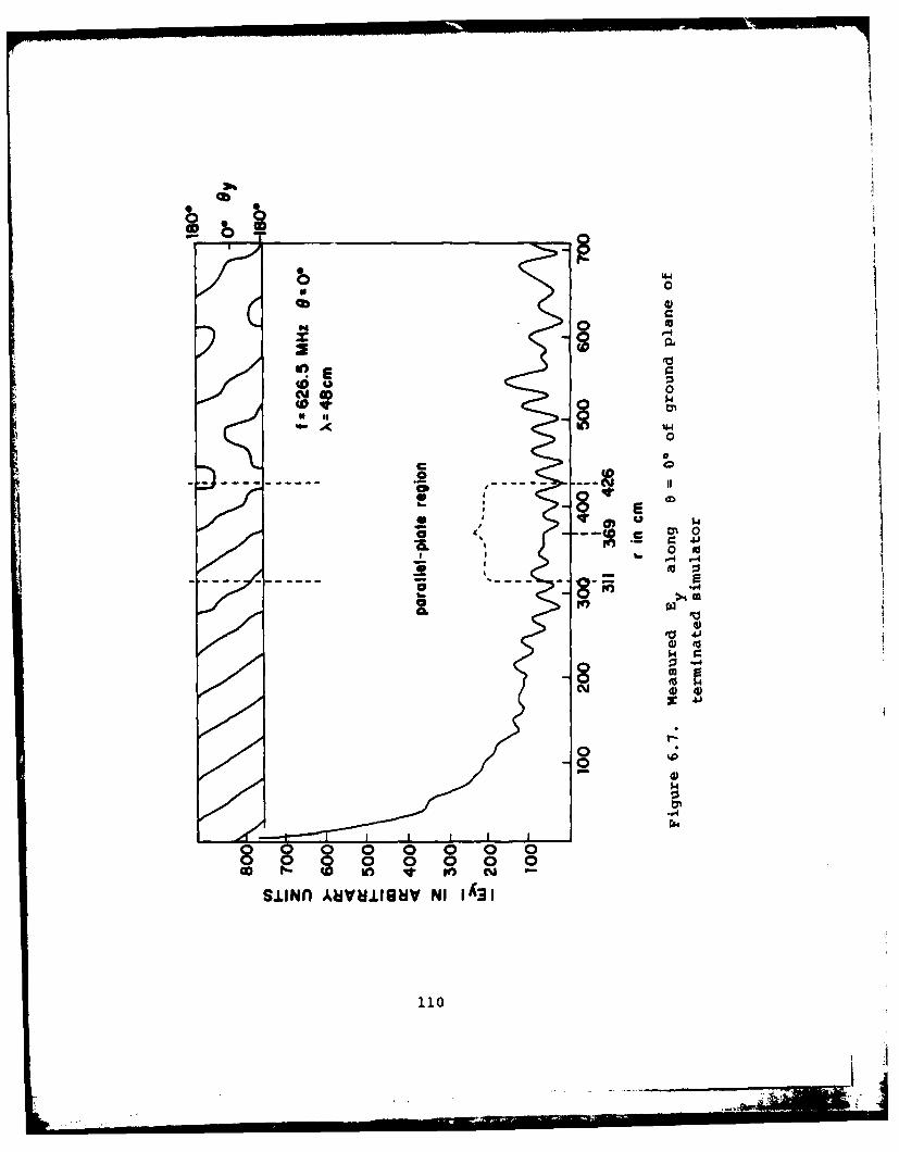
0
0
r-4 0
* IV
41
00
C 00o4
0 i
ra
0 0 000 0
110

structure has the properties of an end-loaded transmission
line operating in the TEM mode with negligible radiation,
low line losses, a constant characteristic impedance, and
a standing-wave ratio determined by the terminating load
impedance. The TEM electric field in the working volume is
vertically directed and approximately independent of the
transverse coordinates x and y at points not too close
to the side edges of the plates where fringing effects occur.
That is, E(x,y,z)= 1 zE y(z). Ey (z) is proportional toV(z), the transmission-line voltage across the conductors.
The planes z - constant are ideally surfaces of constant
amplitude IEy I and phase 6 Y. The incident wave travels in
the positive z-direction, the reflected wave in the negative
z-direction. With a proper termination ZL = zc , the
reflected wave from the load can be reduced to a negligible
value. However, reflections do take place at the discontinui-
ties at the junctions of the parallel plate and the sloping
triangular end plates.
When the frequency is so high that kb is not small,
in particular, when kb = 2nb/X = 4.5w or b = 2.25X as for
the Harvard simulator at the operating wavelength X = 48 cm
and the height b = 108 cm, the electric field in the parallel
plate region is much more complicated. This is true to a lesser
degree when kb = 1.327 or b = 0.66X as for the Harvard
simulator when A - 113.6 cm and b = 75 cm. Owing to the wide
spacing, most of the energy supplied by the generator is now
radiated into the surrounding space, and only a small fraction
is dissipated in the load. The structure is essentially an
antenna and not a transmission line. This has been confirmed
by SooHoo [6.11 in a numerical analysis of a comparable simu-
lator. He concludes that in the high-frequency region the
radiated power approaches 80% of that supplied by the generator.
In order to understand the characteristics of the
measured field and to relate them to the simple TEM field that
k 111

dominates at low frequencies, it is advantageous to have an
at least approximate theoretical representation of the field
in the working volume. Owing to its finite size and connec-
tion to the sloping triangular driving and loading members, the
working volume is not simply a section of an ideal parallel-
plate waveguide of infinite length. No general analytical
treatment of the complete simulator has been made. Analyses
are available of infinitely long, parallel-plate waveguides
with plates that have a finite width that is arbitrary,
Dudley and Quintenz (6.2], Rushdi, et al. [6.3], or that is
very narrow Marin [6.4], very wide Marin [6.5], Marin and
Lewis [6.61, or infinitely wide Marcuvitz [6.7]. None of
these provides any information on the fields in and the
transmission-line properties of the long sloping triangular
sections or of the junction region between them and the
parallel-plate region. Unfortunately, they also provide
primarily qualitative information about the fields in the
parallel-plate section since this is only 115 cm long, but
175 cm wide and (with image) 216 cm (or 150 cm) high. Thus,
the condition of infinite length (or at least great length
compared with the transverse dimensions) implicit in all of
the analyses of parallel-plate waveguides is not satisfied.
Indeed, the parallel-plate section is relatively so short that
end effects can be expected to be significant over much of its
length. Even so, the theoretical representation of the field
in an ideal parallel-plate waveguide in terms of propagating
TEM, TM, and TE modes should provide the best available frame-
work for interpreting the measured field in the working volume
of the model simulator.
VI.5 The Field in the Parallel-Plate Section; TEM and TM Modes
Since the field incident on the parallel-plate section
of the simulator is a spherical wave, it is of interest to
112

determine the nature of the phase fronts which characterize
the electromagnetic field in that section. Measured graphs
of the wave fronts or contours of constant phase, y
constant, of the vertical component Ey of the electric field
in the parallel-plate region when b - 108 cm and f - 626.5
MHz are shown in Figures 6.8a and 6.8b in vertical yz planes
at discrete values of x ranging from x - 1.7 cm near the
center at x = 0 to x = -70.3 cm near the edge at
x = -87.5 cm. Also shown are the wave fronts of a spherical
wave originating at the driving point ( x = 0, z = -369 cm,
y = 0). Clearly the phase fronts throughout the parallel-plate
region are essentially spherical with a superimposed oscillation
due to reflections from the top plate.
It is not convenient to describe the field in a parallel-
plate waveguide in terms of spherical wave fronts originating at
an outside point. The natural representation is in terms of a
superposition of plane waves known as parallel-plate modes. The
simplest form is given by the mode theory of infinite parallel
planes [6.7]. Applicable to the parallel-plate section of the
simulator are the TM modes symmetric in y supplemented if
desired with the more complicated theory for plates of finite
width (6.2 to 6.6]. The significance of TE modes is considered
in a later section. Using the relevant TM modes* given in
reference (6.7] one can write the field quantities for the
various modes.
For the Harvard working volume and with the operating
frequency at f = 626.5 MHz, the TEM mode with n - 0 and
three TMON modes with n = 1,2, 3, can propagate. For the
TEM mode, k k 0.1309 cm-; for the TM On modes,
kgI - 0.977k- 0.128 cm -1 k g2 = 0.893k = 0.117 cm-, and
kg3 - 0.748k = 0.098 cm . The corresponding guide wavelengths
* When referred to the full height with image, b is replacedby 2b, and n = 0,2,4,6,..., instead of 0,1,2,3,...
113
--I III.-. - .- * - -. *1,i.. T..:
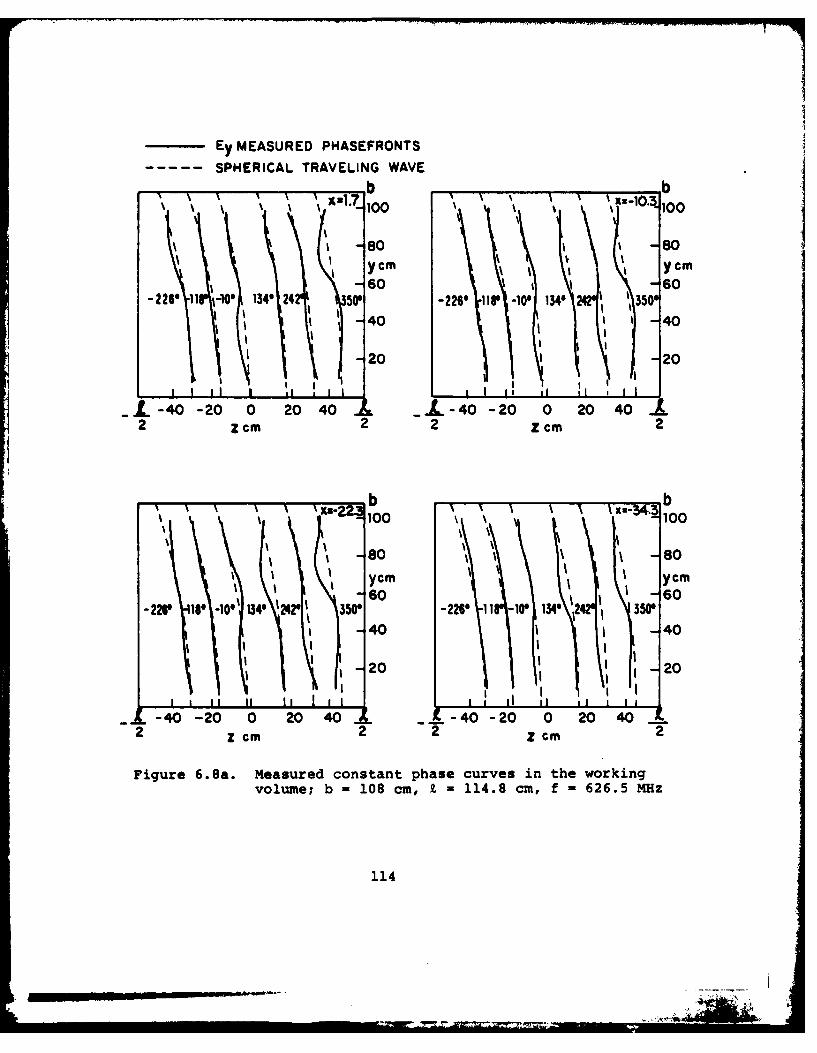
Ey MEASURED PHASEFRONTS
~SPHERICAL TRAVELING WAVE
-80 -80ycm yCM60 I I60
-226' 11 -00 1340 24 50P -2260 1160 -100 1346 3500
I 40 1 1 -40
I20 1 -20
.- 40 -20 0 20 40 -. L-40 -20 0 20 40 12 Z cm 2 2 ZCM 2
x2"b b100 ' ~u3. 100
-80 -80
60 60ro-226' 1$* -100 1'340' 2421 350' -226' 11 -10* 134' 2" 3506 4
-40 -4
1 1 20 I2
- 40 - 20 0 20 40 -40 -20 0 20 42Z C M 2 2 Z cM2
Figure 6.8a. Measured constant phase curves in the workingvolume; b -108 cm, L~ 114.8 cm, f 626.5 MHz
114

EMEASURED PHASEFRONTS---------------SPHERICAL TRAVELING WAVE
x-100 x-5. 1001*80 -80ycm yCM
-~ 60 -60
-226' 18' -10' 1340 24 1 350!' 40 2260 Il8' -10' 1341 242' 350' 40
-20 2
L-40 -20 0 20 40 1 _£-40 -20 0 20 40L2ZCM 2 2 Z CM 2
b-V xz-70.3 100
-80
I \ 60
-226' -110~110 134' 1242' 50 4I I
-40 -20 0 20 40
Figure 6.8b. Measured constant phase curves in the workingvolume; b =108 cm, Z. - 114.0 cm, f = 626.5 MHz
115

are X = g= 48 cm for the TEM mode and Xg1 = 49.1 cm,gO gXg2 = 53.7 cm, and Xg3 = 64.2 cm for the TMn modes. Thefields for the four modes are:
TEM: Ez = 0, Ey = 0.096V 0 (z), Hx = 0.09610(z) (6.1)
TM01: Ez = -ill.41 1 (z)sin(.029y), Ey -0.136V 1 (z)cos(.029y)
= 0.1361 1 (z)cos(.029y) (6.2)
TM02: Ez = -i22.8I 2 (z)sin(.058y), Ey = -0.136V 2 (z)cos(.058y)
Hx = 0.1361 2 (z)cos(.058y) (6.3)
TM03: Ez = -i34.213(z)sin(.087y), Ey = -0.136V 3(z)cos(.087y)
Hx = 0.1361 (z)cos(.087y) (6.4)x 3
The relative amplitudes of the incident and reflected waves for
each of these modes are not readily determined analytically.
However, they can be estimated at any cross section of the
parallel plate region by comparison with the measured field.
The electric field lines characteristic of the TEM and
first three TM0 n modes are shown in the yz-plane in Figure
6.9. At the upper left are the exclusively vertical field
lines of the TEM mode. They have alternate upward and down- Iward maxima at intervals of X/2 = 24 cm. Note that there
is no associated component E . At the upper right are thez
electric field lines for the TM01 mode. These resemble the
TEM mode near the top conductor, but are oppositely directed
near the ground plane since they are parts of closed loops with
an Ez component in the region halfway between the conducting
surfaces. The alternating upward and downward maxima now
occur at intervals of Xgl/2 = 24.6 cm. On the lower left are
the E-lines for the TM0 2 mode, on the lower right those of the
TM03 mode. These have additional closed loops in the vertical
116
- -,-~-

Z in cm Z in cm-48 0 48 -48 0 48
1 I I I I I A I fu ll
TM h , ,TMo
j I I~I I
02M' it01
, I I I I ,I I I I
-48 0 48 -48 0 48Z in cm Z in cm
Figure 6.9. Electric field lines for four parallel-plate modesin workint volume X = 48 cm
117

direction with associated E -components and a wider spacing
between successive maxima in the horizontal direction. Thus,
for the TM02 mode, the maxima occur at intervals of
Xg2/2 = 26.8 cm, for the TM0 3 mode at intervals of
Xg3/2 = 32.1 cm. Axial distributions of the four modes are
shown in Figure 6.10 with an assumed standing-wave ratio of
1.36 for each: Note that for the TEM mode at the bottom,
there are four half-wavelengths in the range -48 cm :. z :. 48
cm, whereas for the TM03 mode at the top, there are only
three half-wavelengths in the same range.
When b = 75 cm and f = 264 MHz or X = 113.6 cm, the
only propagating TM modes are the TEM mode and the TM0 1 mode.
For the latter, the cut-off wavelength is Xc = 2b = 150 cm
and the guide wavelength is Xgl = 174 cm.
VI.6 The Measured Field in the Working Volume:
b = 2.25X = 108 cm; f = 626.5 MHz
The principal components, Ey and Ez , of the electric
field in the working volume were meas red as functions of the
longitudinal variable z with the transverse variables x and
y as the parameters. Consider first the field with f = 626.5
MHz when b = 108 cm = 2.25A and A = 48 cm. (The field with
b = 75 cm = 0.66X with X = 113.6 cm is studied in the next
subsection.)
In Figure 6.11 are shown measured distributions of
Ey I and IEzI in the yz-plane at x = 1.7 cm, i.e., very
near the central plane x = 0 of the parallel-plate region.
The parameter y/b ranges from 0 at the bottom to y/b = 1
at the top. The field along the ground plane y/b = 0 was
measured with the monopole probe mounted on the movable metal
disk; the field along the underside of the top plate was
measured with the monopole probe that moves in the longitudinal
slots. The field at all other values of y/b was measured
with the movable dipole space probe that is supported by a
118

0
-4 q
-4 .
N ~ 0)
4 ~
Pdo 0
0 CC)
co roa))~CODI~ rl)m4
-c; ~ -- ~ -~- ~ 0rrm (D I
4~. 11 FE11 9

3
1 .9I Eyl09l
0 -
-= -- 0.73j
2 0.63
2-
0- 0.54
2-
2 0.17
0- 015m.2426 :10 m:22
12

long tube parallel to the x-axis that moves laterally and
vertically. The component E was measured with the dipoleyin the vertical position, the component Ez with the dipole
in the horizontal position. Only the magnitudes IEy I andEzI are shown in Figure 6.11. Actually, both magnitude
and phase were measured. Furthermore, for each height y/b
shown in Figure 6.11 except y/b = 0, the fields were
measured at seven values of x covering one-half of the
parallel plate region.
Extensive field measurements were made at y/b = 0.08,
0.45, and 0.91 as measured with the space probe and at
y/b = 1 as measured by the monopole probe protruding from the
top plate and have been reported in Wu, et al. [6.81 and
Krook, et al. (6.9]. Of particular interest are the four
graphs of IE I shown in Figure 6.12. They reveal they
striking change in the standing-wave pattern in the plane
x = 1.7 cm from near the top (y/b = 0.91) to the near bottom
(y/b = 0.079). Clearly there are three standing-wave maxima
at thL top, four at the bottom. Actually, the standing-wave
pattern for IEyI at y/b = 0.08 near the ground plane and
shown at the bottom in Figure 6.12 is a good approximation
of the TEM field shown at the bottom of Figure 6.10. The
successive maxima are quite uniformly spaced at X/2 24 cm
and E = 0. On the other hand, the standing-wave pattern
of IE I at y/b = 0.91 near the top plate is quite dif-y
ferent in that there are more nearly three instead of four
standing half-wavelengths in the distance -48 cm S z S 48 cm.
This is shown at the top in Figure 6.12. Thus, the measured
graph at the top in Figure 6.12 resembles the graph at the
top in Figure 6.10 for the standing-wave distribution of the
n = 3 mode in the parallel-plate region. It is also evident
from Figure 6.11 that Ez is significant. It has a standing-
wave distribution with a wavelength near Xg3 and is displaced
from that of IEy I by nearly Xg3/4.
121
. ..I:,,. . ... .. .. .. .._' : .2 ; ,l;; , ' '

CD 0
4~j
4J
E (04Q 4
00
$4
$4
w00
0 Np'-4
00
00 0 0 0
o l 0o 0o 0 0 0
9100S AJDJ4!q.10 1431
122

In order to interpret the extensive data contained inthe measured field in the working volume, the graphs shown in
Figure 6.13 were constructed from the measured data. They
show the measured IE y as a function of the vertical coordi-
nate y at seven different transverse positions x across
the central plane (z = 0) of approximately one-half of the
parallel plate region. The distributions are seen to be
quite comparable in magnitude and shape, thus indicating a
field that is reasonably independent of the transverse
coordinate x, as is implicit for the ideal TEM and TM0 n
components. The fact that E is approximately independentyof x also indicates that the contribution to IE I by possibleyTE0 £ modes is small. This is considered in a later subsection.
At each cross section (z = constant), E can beyapproximated by a superposition of the TEM and the three
propagating TM On modes. The relative amplitudes of these
modes cannot be determined theoretically, but can be obtained
from the measured distribution of Ey. This superposition ofy
modes has been demonstrated in Figures 6.14a and 6.14b.
It is evident from these figures that the assumed
approximate representation of the field as a superposition of
the ideal parallel-plate TEM and TMn modes is a good one
throughout the working volume of the model simulator. It is
also evident that the total E differs greatly from theypart contributed by the TEM mode alone, which is constant in
y. Such a representation has also shown that the amplitudes
of the TEM and TM0 1 modes are almost the same. Their standing-
wave distributions and phases are such that JE yI is sub-
stantially greater near the top plate, y = b, than near the
ground plane, y = 0.
123

OR 00
0 C5
-00-
14
Ul) u
0* 1
0 ".0
Iw 0
0 0
.2 GiI
0 44U
0J I00
Ire)
C .000
~r,0~ 00
to N
1244
0 -Etotp
W)t

cn
0W I 0m
LA011-.
LAJ.1c 0.,1
-
"4
"4>9
4-4
40
044
oo :
$40
'U-00)
to 'U
1251

00 o
0
ONN
00
ODO
II
E 0
H.4.-
/ - 'S 1.4fA

VI.7 The Measured Field in the Working Volume:
b = 0.66X = 75 cm; f = 264 MHz
The components Ey and Ez in the working volume and
adjacent regions were also measured with f = 264 MHz when
b = 75 cm = 0.66X and X = 113.6 cm. To simplify the pre-
sentation of the data, these components of the field were
measured as functions of y/b with z = 0 and x as
parameter. The measured graphs of IE , IE Jz, e and ey z y Zare shown in Figure 6.15 for eight values of x.
As with the higher frequency and greater height b
of the working volume, the approximate representation of
Ey and Ez by TEM and TM On modes was found to be quite
satisfactory. The difference is that at f = 626.5 MHz,
it took 3 TM modes, whereas at f = 264 MHz it took only
the TM01 mode in addition to the TEM mode for adequate
representation of measured fields.
VI.8 The Transverse Variation of the Electric Field;
TE Modes
The approximate representation of the electric field
in the parallel-plate region of the simulator in terms of the
TEM and TMOn modes tacitly assumes that all of the components
of the electromagnetic field are independent of the trans-
verse variable x since all wave fronts are assumed to be
planes perpendicular to the longitudinal z-axis. This was
taken to be a good approximation because the electric field
shown in Figure 6.13 changes relatively little as x is varied
in steps from near the center of the parallel plate region to
near the edge at x = ±a = 87.5 cm. By examining the varia-tion of the field with the x-coordinate in great detail, we
have basically concluded that the contribution of TE0t modes,
if any, is negilgible at both frequencies (626.5 MHz and
264 MHz) compared to the combined contribution of TEM and
127

150 -0 7 - 1800
x:0 -10.5 -21 -31.5 lEyl -21 -10.5 -31.5 goo100 V0
EI Xu0 -10.5 -21 -31.5-50 e - 4- _90
501. -1800
U) 0
Cr 150 7 -8 703=SL 1800
Cr 100-Iy
50 43.7 -58.3 -70.3 -82.3 -82.3 -70.3 -43.7,- -
'-83-900
01000 0.5 .
Figure 6.15. Measured electric field in transverse plane z = 0of parallel-plate region; 2.k 114.8 cm, 2a 175 ci".,b =75 cm, f =264 MHz
128

TMOn modes. This conclusion was reached starting with the
nature of the wavefronts or the surfaces of constant phase
in the parallel plate region and recognizing this to be a
traveling spherical wave with superimposed oscillations due
to standing waves. The incident spherical wave can excite
antisymmetric components of H and can potentially excite
antisymmetric TE0 £ modes. The amplitudes and wave members
of TE0v modes are known [6.3] for certain dimensions. From
examining the data, it is reasonable to suppose that a
superposition of TE0o modes will account for the difference
E y(x,y,z) - Ey (O,y,z) where Ey(O,y,z) is the field
represented by TEM and TM0 n modes, and to assume that the TEll
mode contributes negligibly. For the present purpose of this
section, the representation of the electromagnetic field in
terms of TEM and TM On modes is adequate without the addition
of a sum of TE0 £ modes, because it is experimentally verified
that the departure of E y(x,y,z) from Ey (O,y,z) is quite
small--on the order of 8%--in the central part of the
simulator.
VI.9 The Actual Electromagnetic Field in the Simulator as an
Approximation of a Plane Wave
The electromagnetic field which is to be approximated
in some volume of the simulator is a plane wave traveling in
the positive z-direction with the components E (z,t) =i~zw)Y 1/2E y(0)ei(kzt), Hx(z,t) = E y(Zt)/C 0 where /0 = 20/E0
= 120v ohms. The field is independent of the transverse
coordinates y and x, and is distributed as shown in the
upper left of Figure 6.9 at the instant t = 0. As time
passes, the entire pattern moves in the positive z-direction
with the speed c = 3 x 10⁸ M/sec.
129

The actual field in the parallel-plate section of the
simulator is a spherical wave originating at the driving-point
on the ground plane and modified by superimposed reflections
from the top plate. The field can be approximated by a sum
of appropriate parallel-plate modes, but this is merely a
change in the representation and not in the nature of the
field. Moreover, all of the modes are generated by the
incident field and not by reflection at load end.
As the cylindrical wave travels in the parallel-plate
region, it experiences reflections at the edges x = ±a and
at the end z = £/2. The former maintain the transverse
standing waves, the latter the longitudinal standing waves
like the one shown in Figure 6.11. They can be decomposed
into separate standing waves of the TEM and TM On modes for
the E and E components. Measurements were also madeyof the standing-wave pattern of the magnetic field over a
wide range of frequencies centering on f = 264 MHz with
b = 75 cm. Selected graphs at f = 250, 264, and 270 MHz
are shown in Figure 6.16. It is seen that as the frequency
is varied, the entire standing-wave pattern moves. Simul-
taneously, the standing-wave ratio fluctuates. Note in
Figure 6.16 how the depth of the minimum varies as its loca-
tion moves. If the loop probe is fixed at z = 0.074£ = 8.5
cm, which locates the minimum for f = 264 MHz shown in themiddle figure in Figure 6.16, and the frequency is then varied,
the graph shown in Figure 6.17 is obtained. This shows a
succession of minima that occur at z = 0.074£ at different
frequencies, but with that at f = 264 MHz the deepest and
sharpest. The maxima and minima in Figure 6.17 are a conse-
quence of the standing waves generated in the working volume
by reflections of the field at the ends z = ±X/2 and the
adjacent tapered sections. The standing-wave ratio varies
somewhat with frequency so that the minimum amplitude at any
fixed point increases and decreases with frequency. The
L . .130

1.0 180 °250 MHz
0.5 IH ' 0.2
01 I - -- 1800
1.0 ,1800
264 MHz. IHx,(-O.l2a,O z)j
0 00
OHx
I 1 ,.18001.0 .074b 270 MHz 10
IHx(-O.12aOz)l
0.5 - - 00OHx
0,-0.2 0.19
Z scale
Figure 6.16. Measured manitude and phase of the transversecomponent of the magnetic field on the ground
plane
in the working volume; width 2a = 175 cm, lenth
X = 114.8 cm, height b = 75 cm
131

+6dB
Od8 N
H, 0.o12a,0,0O.074f.)J
-2OdB -
-30dB'
250 260 270 280 290 300 310 320 330 340 350
Frequency in MHz
Figure 6.17. Measured magnitude of the transverse magnetic fieldat a fixed position in the working volume as afunction of frequency; 2a = 175 cm, £ = 114.8 cm,b = 75 cm, Pf = 40 w
132

deepest minimum at z = 8.5 cm occurs at f 264 MHz. At
another location of the probe, the frequency for and the
depth of the minimum will be different.
The differences between the actual electromagnetic
field in the working volume of the model simulator and a
traveling plane wave are significant when b = 108 cm = 2.25X
with f = 626.5 MHz and considerably larger when b = 75 cm =
0.66X with f = 264 MHz. In the first place, the component
E of the electric field is not uniform in either theytransverse or vertical directions; second, there is a small com-
ponent Ez; and, third, there is a significant standing wave.
It follows that the electrical environment of a metallic
obstacle placed in the working volume is necessarily quite
different from what it would be if it were exposed to an
incident plane wave. Therefore, it must be expected that
currents and charges induced on the surface of an obstacle may
also be quite different. A detailed comparison of the distribu-
tions of induced currents and charges on obstacles when in the
simulator and when exposed to a plane wave will be investigated
in detail and reported at a later date. For purposes of com-
parison, theoretically determined distributions of Burton,
et al. [6.101 are available. Although some sample set of
measurements has been made of the very sensitive charge density
distribution on the surface of a tubular cylinder located at
the center of theparallel plate region, it is considered use-
ful to postpone such comparisons until more extensive experi-
mental data become available.
VI.10 Possible Methods to Improve the Field in the Simulator
as an Approximation of a Traveling Plane Wave
The lateral and vertical nonuniformity of the field in
the simulator on the one had and the existence of standing
waves on the other hand constitute the principal departures
133

from the desired traveling plane wav. Of these the first
is a consequence of the spherical wave fronts that are
incident on the parallel-plate section, the second is due
to reflections at and beyond the junction of the parallel-
plate region and the tapered section leading to the termina-
ting impedance.
It might be supposed that the nonuniformity in the
transverse distribution of the electric field is a problemonly at high frequencies when modes other than the TEM can
propagate in the parallel-plate section. The cut-off wave-
length for the TM01 mode is cl = 2b so that at all wave-
lengths longer than 2b only the TEM mode can propagate.
However, with the length z(= 216 cm or 150 cm) and, there-
fore, less than X when this is greater than 2b, even non-
propagating modes may have significant amplitudes in the
electrically rather short parallel-plate section. One wayto reduce the transverse variation in E in the parallel-Yplate section is to provide an incident field that more
nearly approximates a plane wave than does the actual spherical
wave. With the geometry of the input structure predetermined,
this is not readily accomplished. It involves a modification
of the phase velocity of the spherical wave in the tapered
section from the generator by some kind of a collimating lens
or its equivalent in the form of metal plates or corrugations
on the ground plane so that the spherical wave front becomesmore nearly planar as it reaches the parallel-plate section.
The existence of standing waves in the parallel-plate
section is a consequence of the fact that the entire structure
has the characteristics of a terminated transmission line only
at low frequencies for which the condition 27b/<< 1 is
satisfied. This condition underlies the theory of all open
transmission lines, and requires that radiation be neglibible
in determining the characteristics of the line. When this
condition is satisfied, it is possible to design the trans-
134
I .. ....... ... . .. .. ..

mission line so that virtually all of the power supplied by
the generator is transmitted along the line to a matched load
at the end. As the height b is increased, radiation becomes
significant and, for sufficiently large values of b, dominant.
The structure then acts like a traveling-wave antenna. Since
the standing-wave ratio in the parallel-plate section is reason-
ably constant (see Figure 6.11), it is evident that the effective
load on the open parallel-plate waveguide is at or beyond its
junction with the sloping triangular plate at the load end.
That is, most of the radiation takes place during reflection
at or beyond the discontinuity formed by this sharp junction.
(It is to be expected that radiation also takes place at the
junction of the sloping triangular plate with the parallel
plate at the generator end, but this does not affect the
standing-wave ratio in the parallel-plate region.)
It was seen that the amplitudes of the TEM and TM0 1modes are about equal and those of the TM0 2 and TM modes
negligible when b = 2.25X = 108 cm with f = 626.5 MHz.
In this case, the standing-wave ratio as obtained from
Figure 6.11 is less than 2. On the other hand, the amplitude
of the TEM mode exceeds that of the TM01 mode when b = 0.66X
= 75 cm with f = 264 MHz and in this case the standing-wave
ratio is about 3. It, thus, appears that the standing-waveratio in the parallel-plate region can be reduced signifi-
cantly only by reducing the reflection at y Z b/2 of the
entire component E on the electric field between they
parallel plates. The selective reduction of the TM On modes
by attenuating Ez, even if 100% successful, would not
significantly reduce the standing-wave ratio when it is greatest,
if the TEM wave is not properly terminated. There is no com-
parable way to attenuate separately the TE0 Z modes since they
have only an Ex component of the electric field. What is
required to reduce the standing-wave ratio is more frequency-
dependent termination for the parallel-plate section of the
135
I.

simulator than is provided by the sloping triangular plate
with its resistive termination, which is frequency
independent only at sufficiently low frequencies. This is
important primarily in the intermediate range of frequencies
when b is of the order of a wavelength and the standing-
wave ratio is higher. More work in optimizing the terminator
is planned, and it is expected that a combination of a proper
load and selective reduction of TM On modes will significantly
minimize the reflection problem.
136

VII SIMULATOR/OBJECT INTERACTION
VII.1 Introduction
In designing new bounded wave EMP simulators, or in
assessing the measured data obtained from existing simulators,
it is important to determine to what extent the presence of
the simulator structure affects the response of the test
object. The usual objective of a simulation test is to
evaluate the response of a system, say an aircraft, in the
in-flight or ground-alert modes with no simulator facility
present. This is usually not possible due to the need for
providing high electromagnetic energy densities in the vicinity
of the test object. This requirement generally leads to
locating the simulator structure close to the system being
tested thereby increasing the degree of simulator/object
interaction. For the in-flight mode of testing, in addition
to the conductors, dielectrics, wires, etc., that make up the
simulator, the nearby ground should also be electromagnetically
invisible during the time when the test object is responding.
In this sense, the ground effects can also be categorized
under simulator/object interaction.
Although bounded wave simulators are constructed with
conducting parallel plates (approximated by wire meshes in
practice) having a finite width, the analysis of the behavior
of objects within the simulator is usually simplified by
considering an infinite parallel-plate region containing the
object. Thus the simulator/object interaction problem is
reduced to that shown in Figure 7.1, where a doubly infinite
set of images may be introduced to account for the presence
of the parallel plates. The answer to the question of how
the response (probably both in time and frequency domains) of
the aircraft in Figure 7.1 differs from that of the aircraft
in free space then serves to quantify the degree of simulator/
object interaction.
137

a
Imaqes
Incident fField k Object under test
Imaqes
Figure 7.1. Object under test and images in parallel plateEMP simulator
138
I __________________

A number of studies have been performed in an attempt
to describe simulator/object interaction. Since it is
difficult to compute the response of an actual aircraft in
free space (not to mention the case of an aircraft in the
parallel-plate region), investigators have been forced to
consider relatively simple objects, such as cylinders and
spheres, for their studies. Numerous data are available
for these special cases, but nevertheless, there appear to
be a few formalized conclusions that may be drawn from the
past work. This is due principally to the fact that there
is no single quantity which adequately describes all aspects
of object/simulator interaction.
VII.2 SEM Representation
Past studies have dealt with currents at various points
on the object and charge densities (or charge enhancement
factors) in both the time and frequency domains, as a function
of the many geometrical parameters describing the problem.
These studies are documented in references (7.1 to 7.9].
In an attempt to obtain a relatively simple set of quantities
to describe the interaction, the concepts of the singularity
expansion method (SEM) have been applied in reference [7.10]
and, more recently, in reference (7.11]. In the SEM repre-
sentation, the total current at a point E on a thin cylinder
within the parallel-plate region can be expressed as
R~ R ()I(;s)= + + R (7.1)
(s(s-iR
where s represents the complex frequency, s are the
complex natural resonances of the wire, R ( ) is the residuethor pole strength at the a resonance, and IR(&,s) is a
remainder term which arises from both the incident waveform
singularities and the branch cut integrals which arise in
the parallel plate region (7.111. The bar over a quantity
139
J il .. .. ,,,, . L :. .-.- NAME= iJ ..

as in i ) denotes the complex conjugate of the quantity.The second term in the summation with complex conjugate
quantities is required so that the time domain response
I(E;t) will be a real function of time.
In studies to date, attention is focused on the natural
resonances, s. , and how they vary with changes in the
simulator/object geometry. Early studies involved removing
one plate of the simulator and examining the trajectories
of the resonances in the complex frequency plane. Figure 7.2,
taken from reference [7.12], shows the trajectories of the
first two resonances of a thin cylinder of length L and
radius a , which is parallel to the bottom plate, as a
function of height, d , of the cylinder. As is noted,
substantial variations of the damping constants are obtained
for the first natural frequency. For this particular example,
the length to radius ratio was L/a = 200
Similar data for the first resonance have been presented
in reference [7.91 for the same thin wire at various inclination
angles, S . Note that a = 00 implies that the wire is
parallel to the ground plane, and B = 900 is for the wire
perpendicular to the ground. Figure 7.3 shows the percent
change of the first resonant frequency relative to the free
space value, as a function of the height of the wire (measured
from the wire midpoint) above the ground. Figure 7.4 shows
the corresponding variation of the damping constant. Although
these data are in a slightly different form than the trajectories
of Figure 7.2, they contain essentially the same kind of infor-
mation regarding the simulator/object interaction.
The removal of the top plate of the simulator causes
a significant simplification in the numerical treatment of
simulator/object interaction studies. It removes, however,
an important feature of the problem: that of branch points
within the complex frequency solution for the body response.
140
_ _ _ __ _ _ _ _ _ _ _

(L/6-2001O25 12
1.2.5
-0.? -06 _Q5 -Q4 -OLS -0. -0.1 (10
(a)
1.3
6.2A-10.6
06 (Free Spmce)
f0s . 6.0
1.0 0.8 0.1 -5.9
O(A".9 _5.6
0.3
-0.4 -0.5 0.4 -0.3 -0.2 -at 0.0
(b)Figure 7.2. Trajectories of the first (a) and second (b) naturalresonances of a thin wire of length L and radius a - L/200,as a function of the height of the wire, d , over a conductingground. (The wire is parallel to the ground, and this figureis reproduced from (7.12].)
141

25' a .3o"
20
1.0 :W
0-5
-10
-15
-20
-2.5 ---0 2 4 6 0 12 "4 16 I. 2.0 2224
d/L
Fgiure 7.3. Plots of percent changes of first resonantfrequency of wire object relative to free-space resonantfrequency, shown as function of d/L for various inclinationangles
!4
TI t.i , • I , i • ,
12
10
6
4
2
0 J I i p p p I i5O 10s 20 25
d/LFigure 7.4. Plots of normalized damping constant T/T. forfundamental resonance, shown as a function of d/L forvarious inclination angles. The quantity T. is the free-space damping constant
142
____ _ _I '

In reference [7.5], a study of the thin-wire object within
the parallel-plate region was reported. Although other
authors had considered similar problems [7.2 and 7.3], this
report (7.51 was the first to consider the cylindrical
object to be of an arbitrary angle within the simulator.
Figure 7.5 shows the input conductance of a center-fed
cylindrical antenna as a function of plate separation, d
and for various angles of inclination, e . The discon-
tinuities in these curves at certain plate separations are
due to the presence of the branch points in the s-plane.
For the thin wire perpendicular to the plates, (e = 90*),
note that these discontinuities vanish, suggesting that the
branch point contributions become small or, perhaps, vanish.
Similar discontinuities have been noted for scattering problems
within parallel plates.
In an attempt to understand the behavior of thin
cylinder objects within a parallel-plate simulator from
an SEM view, reference [7.11] presents a study of the
locations of the natural resonances for wires of varying
aspect ratio (a/L) and for three different heights above
the bottom plane. In obtaining these results, an integro-
differential equation is derived, but it is only solved
approximately so that it is difficult to assess the accuracy
of the solution. Moreover, it does not give insight into
the degree of importance of the branch point contribution
to the solution. It does provide, however, a first step
at applying SEM concepts to this interaction problem.
The results reported in [7.11] are briefly summarized in
the following Tables numbered 4.1, 4.2 and 4.3. In these
tables, the pole locations in the complex s-plane for the
three cases of L/d = 0.2, 0.5 and 0.8 are presented. It
is noted that the cylinder is located symmetrically in the
parallel plate region with its axis normal to the plates.
143

14
I
01011 i\l i~
160
4 -6-00 .... 30:
00
I
0 15 to 1.5 2o 2. 3.0 3.5 4.0d [in]
o c e ivn \X n L)
CO-8 1 0 =i 1 00o
.. . 300
-120. 15 .0 1.5 2.0 2. 3.0 3.5 4.0
d [i n X.]
Figure 7.5. Input conductance (top) and susceptance (bottom)of a center driven antenna (L=X/2, Q=2 n (2L/a) = 10) locatedat a distance h = d/2 from the bottom plate of a parallel-plate region of separation d . The arrows indicate the free-space values 144
iwww i

TABLE 4.1
POLE SINGULARITY PARA.IETERS FOR L/d = 0.2
s'L s"Lm a m mL Tr Tr'6
0.003 -0.085 0.935
0.01 -0.114 0.927
0.03 -0.162 0.917
0.1 -0.290 0.918
0.003 -0.117 1.91
2 0.01 -0.160 1.910.03 -0.238 1.91
0.1 -0.460 1.98
0.003 -0.138 2.90
0.01 -0.192 2.90
0.03 -0.293 2.91
.1 -0.578 3.09
0.003 -0.154 3.89
0.01 -0.217 3.89
0.03 -0.337 3.92
0.1 -0.647 4.22
0.003 -0.167 4.88
0.01 -0.238 4.89
0.03 -0.374 4.94
0.1 -0.674 5.33
0.003 -0.179 5.88
6 0.01 -0.257 5.89
0.03 -0.406 5.95
0.1 -0.671 6.42
145

TABLE 4.2
POLE SINGULARITY PARAMETERS FOR L/d =0.5003
slL s"Lm M
0.003 -0.052 0.952
1 0.01 -0.064 0.950
0.03 -0.081 0.950
0.1 -0.109 0.963
0.003 -0.126 1.94
0.01 -0.174 1.932
0.03 -0.266 1.91
0.1 -0.557 1.99
0.003 -0.094 2.90
0.01 -0.119 2.91
0.03 -0.15s 2.93
0.1 -0.186 3.03
A0.003 -0.16S 3.930.01 -0.236 3.92
0.03 -0.379 3.93
0.1 -0.848 4.27
0.003 -0.117 4.88
0.01 -0.152 4.90
0.03 -0.199 4.95
0.1 -0.176 5.10
0.003 -0.191 5.92
6 0.01 -0.280 5.92
0.03 -0.458 5.97
0.1 -0.976 6.61
146
_________

TABLE 4.3
POLE SINGULARITY PARAMETERS FOR L/d = 0.8003
s'L s"La m mm L- c
0.003 -0.114 0.956
0.01 -0.154 0.947
0.03 -0.226 0.936
0.1 -0.431 0.952
0.003 -0.128 1.97
2 0.01 -0.177 1.97
0.03 -0.266 1.99
0.1 -0.504 2.15
0.003 -0.110 2.97
0.01 -0.151 2.98
0.03 -0.220 3.01
0.1 -0.327 3.21
0.003 -0.061 3.95
0.01 -0.075 3.96
0.03 -0.090 3.98
0.1 -0.065 4.04
0.003 -0.129 4.88
0.01 -0.180 4.87
0.03 -0.270 4.88
0.1 -0.447 5.02
0.003 -0.182 5.86
6 0.01 -0.265 5.85
0.03 -0.435 5.86
0.1 -1.25 6.22
147

Comparisons of the pole trajectories of cylinders in the
parallel plate region with those of isolated cylinders,
as well as comparisons of time doman responses, should
be pursued in future efforts.
VII.3 Fields Near the Test Object
Another approach in understanding how an object inter-
acts with the simulator is to investigate the behavior of the
electric fields in the vicinity of the test object. These
fields generally have four components, 1) fields produced by
currents flowing on the test object, 2) fields produced by
currents flowing on the parallel plates (i.e., the image
currents), 3) the incident field, and 4) reflections of the
incident field within the parallel-plate region. The
fourth field component is often neglected, since pure TEM
excitation is assumed. Concentrating on the first two field
components, it is noted that their behavior depends not
only on the overall body geometry, but also on the simulator
geometry. For the thin wire of length L , analyzed in
reference (7.5], an integral relation for the scattered
electric field at a point [ is given by
Lj ,. inc (- f I(') [Kfs(,';)+ Kp,
0(7.2)
inc-where Ei( ) is the incident TEM field, I(T') is the
induced wire current, Kfs is a free-space kernel and Kppis the additional contribution to the kernel which takes into
account the presence of the parallel plates. This relation
may be used to derive an integral equation for the wire
current. A study of the variation of the K term relativeppto K fs will thus permit some insight into the interaction
problem.
148
I._

In order to assess the relative importance of these
terms, it is possible to study the magnitude of the ratio
K pp/Kfs as a function of the height of the scatterer above
the bottom plate with all other variables taken to be constant.
This is equivalent to investigating the primary and image
components of the electric field which are parallel to the
wire at a position C , due to an infinitesimal current
element at a position E' . To minimize the complexity of
this problem, we consider both and E' to be located
at the midpoint of the wire, i.e., at L/2 , and the wire
to be inclined with an angle e = 900 , which provides for
maximum interaction with the ground plane. Figure 7.6 shows
the geometry of this case. From [7.5], the free-space kernel
has the value
K (L/2,L/2;w) = + k2 ) 2
4 [( ' + a I E=E'= L/2
(7.3)
where a is the radius of the wire and k = w/c The
portion of the kernel due to the parallel plates is given by
-jkR(1 )
+ 2 e n
K (L/2,L/2;w) = k - cos(24R(n=-c ) n
4jkR (2)n=-n+(+2 ) (2)
=_04Tr R
n#0
(7.4)
where
149
Oi4 40'-Tq

Images
-~ e -,Physical
d Space
* rhImages
Figure 7.6. Infinitesimal current element within parallel-plate region
150
OWN"

(i [((L--') sine - 2(h+nd)) + ( - ')cose]Rn
(7.5)
(2) [(((-E')sine - 2nd) 2 + ((E-V')cose) 2]n (7.6)
and d is the plate separation and h is the height of the
source point above the bottom plate.
A careful examination of the self-kernel in equation3
(7.3) shows that there is a (ka) dependence which tends
to mask the effects of the parallel plates. Thus, it is3
advisable to plot the quantity (K pp/K fs)/(ka)
Figure 7.7 shows this quantity as a function of kd for
various values of source height. The effects of the
resonances introduced by the parallel-plate geometry are
clearly illustrated at kd = 7, 27, etc.
Unfortunately, this measure of object/simulator inter-
action depends on a parameter of the object, namely a
the radius of the wire. It would be possible to plot only
the term JK I which is independent of a , but its valuepp
relative to IKf I is what is important in equation (7.2)
in determining the effects of the interaction. Thus, in
performing a study of this sort, it is important to have a
knowledge of the size of the object, as well as the dimensions
of the parallel-plate region.
In summarizing the past work in this area, it is found
that there is no one scalar parameter which can be used to
describe simulator/object interaction. Given existing
analytical and numerical methods, it is possible to analyze
a few specific obstacles within a parallel-plate region, but
it is difficult to then cast these numerical results into
design curves which would be useful to engineers. The SEM
151

1000 1 I
Ii h/d = .05 .
I .3
.5
100 % a/d= .001I .Kp
I I(ka) 3Kf
Note: Although the plotted quantityI 'does not quantify simulator/
object interaction, it is10 indicative of the degree ofinteraction.
0 0.
I + l'j'"\I
(kd)
.01- ' I I
0 3 6 9 12 15
Figure 7.7. Plot of the normalized ratio of kernels for aninfinitesimal current element at 8 = 900 (parallel to plates)and at a height h ,as a function of plate separation
152
-I.-. - - -. -

concepts, which have been used to explore the shift of the
natural resonances of an obstacle, should be extended
to investigate the effects of the branch points, which give
rise to the discontinuities shown in Figure 7.7. Also, it
is suggested that studies in the variations of the residues
of the natural resonances be made to further understand the
interaction problem. Finally, it would be useful to consider
more realistic bodies within the simulator, say, a crossed-
wire aircraft model.
153
i _

VIII SIMULATOR AS A WHOLE
Because of the complexities in analyzing or
evaluating the performance of the simulator as a whole,
emphasis in the past has been rightfully placed on the
individual components of the simulator. However, it is
imperative that the understanding of various components of
the simulator be hybridized wherever necessary, so that one
can arrive at some meaningful conclusions, with regard to
the simulator performance as a whole. A good example of the
need for such confluence of understanding of individual
simulator components lies in the junction of the conical and
cylindrical (two-parallel plate) transmission lines. We
have a detailed knowledge of the spherical TEM wave character-
istics in the conical plate region [Section III] and the TE,
TM and TEM wave characteristics in the parallel-plate region
(Section IV]. But, at the junction of these two transmission
lines, the fields can be quite complex due to reflections
caused by field mismatches even though the impedance of the
principal TEM modes in the two regions may be matched within
a few percent.
Based on the considerations similar to the above
example, it may be argued that while viewing the simulator as
a whole we are confronted with the problem of assuring smooth
electromagnetic transitions between various components, and,
also between the various stages within a component (e.g.,
monocone switch and Marx column in the pulser).
Many examples of problem areas in this regard were
identified by Baum, Giri and Chen (8.1] who updated a similar
list in an earlier memo by Baum (8.2]. In what follows, we
shall list and briefly discuss these problems, while pointing
out some of their salient features.
154

VIII.l Problems List
1. Characterization of the pulser and improvements
in its matching with the simulator,
2. Evaluation of the TEM mode coupling coefficient
for conical-cylindrical transition in frequency
and time domains,
3. Analysis of TEM and higher order modes in non-
flat plate geometries, e.g., circular arcs,
4. Accurate calculation of the earth effects on
existing simulators,
5. GTD analysis of the simulator as a whole,
6. Determination of the properties of wire grid which
make up the simulator plates for various unit
cell geometries,
7. Higher order mode calculations in the conical
plate region,
8. Appropriate modifications of the wave launcher
and receptor for analysis purposes, consistent
with problem (3) above,
9. Analysis and evaluation of both sloped and
perpendicular distributed terminators for the
case of finitely wide plates,
10. Determination of the properties (attenuation, phase
shift, etc.) of the periodic array of dielectric
rods, metal bolts and rings in the trestle,
11. Determination of simulator distant fields at low
and high frequencies.
155
A

VIII.2 Brief Discussion of Salient Features of ListedProblems
1. Matching of pulser to the simulator
It is fair to state that the pulse power has not
yet received sufficient attention from an electromagneticpoint of view [8.3]. Some of the problems here are: a)
impedance and field matching of the monocone switch geometry
with the Marx and peaker assembly, b) minimizing dispersion
times (8.4] at the Marx-simulator plate interface. Work is
in progress in this area which looks at the Marx type of
pulser as an EM boundary value problem by modeling the
central Marx column along with the peakers as coupled trans-
mission lines.
2. TEM coupling coefficients
The spherical TEM wave fields in the conical region,
are well known in the spherical coordinate system which is a
natural coordinate system for this geometry. From these
studies, the rectangular components in a transverse plane at
the conical-cylindrical junction can be evaluated. These
fields can be thought of as "input" to the parallel plate
region. By matching the fields from the conical region to
those of the parallel plate region at the junction, the TEM
coupling coefficients can be evaluated.
3. Nonflat geometries
For future generation simulators, it is desirable to
explore other top plate geometries, e.g., curved (inwards
[8.5] and outwards) in terms of the propagating modal (TEM,
TE, and TM) distributions, impedances, etc. An important
criterion here is the confinement of energy in the working
volume, coupled with suitable modifications in the wave
launcher and receptor sections.
156
I A

4. Earth effects
Earth moving and sloping techniques have been used
in the simulator facilities to reduce the adverse earth
effects. For example, at frequencies above 5 MHz in ATLAS I
(TRESTLE), the earth effects are not so significant; but
below 5 MHz, more accurate calculation and experimental
validation of such effects for various samples of Albuquerque
soils are useful.
5. GTD analysis
At sufficiently low frequencies, quasi-static con-
siderations apply and the evaluation of working volume fields
are relatively straightforward. At the other end of the
frequency spectrum, where critical dimensions of the simulator
become several wavelengths, ray-optic techniques become
applicable and hence a complete GTD analysis is desirable.
The chief goal of such studies would be the prediction of
working volume fields.
6. Wire grids
Although the simulator plates are in practice made
of wire meshes, analyses and laboratory model studies
have always employed solid plates with zero surface impedances.
If one neglects ohmic losses, the wire-mesh plates have
reactive surface impedance. The effects of this on wave
propagation in conical and parallel plate regions need further
investigation.
7. Non-TEM modes in conical transmission lines
We have extensive data from recent efforts at
Dikewood Industries on the properties of TE and TM modes in
157
parallel plate regions which are summarized in Section IV.
A similar analysis of the conical plate transmission line
will significantly enhance our understanding of the simulator
performance. The conical transmission line is a radial
transmission line and classical methods of determining the
non-TEM modal distributions should be explored.
8. Wave launcher/receptor
If nonflat top plate geometries are considered for
analysis purposes, it is imperative to modify the wave
launcher and receptor sections. Such modifications need to
be addressed with the view of ensuring smooth transitions
for wave transport, at all junctions.
9. Distributed terminators
Lumped resistive terminators with their inherent
intrinsic reactances have been traditionally employed and
experimentally evaluated 15.6]. Furthermore, the desirability
and implications of perpendicular and sloped distributed
terminators [5.4 and 5.5] were considered in Section V on
terminators. However, the available calculations are for
the case of infinitely wide plates, and the case of the
finite width is considered a logical and useful extension of
existing results.
10. Trestle effects
References [8.6, 8.7 and 8.8] consider the problem
of scattering of a plane wave incident on a two dimensional
periodic array of infinitely long dielectric posts. The con-
clusion there was that the support structure reflects little
energy in the low frequency limit, but reflections are non-
neglibible when lengths of wood arrays become comparable to
158

wavelength. Additional complexities are introduced by metal
on the trestle [8.91. More work is desirable in this area by
considering semi-infinite and finite vertical arrays of posts
including horizontal and diagonal cross members. The plat-
form or the trestle top affects the wave propagation and they
can be evaluated at least initially, on laboratory model
parallel plate simulators.
11. Distant fields
Some crude results are currently available [8.10 and
8.11] in estimating the distant fields from this class of EMP
simulators. Reference [8.10] starts with the estimated work-
ing volume fields and computes distant fields via considerations
of (l/r) fall off, reflection and surface wave losses. Also,
at low frequencies [8.11] one can estimate the distant fields
by first estimating the equivalent electric and magnetic dipole
moments of transmission lines formed by simulator plates. In
contrast with high frequency distant fields, it was found that
at low frequencies the maximum radiation occurs in a direction
opposite to the direction of propagation in the simulator. The
available approximate results indicate that more detailed
studies for a wide range of frequencies are desirable.
159
.........

REFERENCES
Most references cited in this report are from theAFWL EMP Notes and Memos series edited by Dr. C.E. Baum.
They have been identified simply as "Sensor and SimulationNote XXX" or "ATLAS Memo XX," for convenience. While copies
of the "memos" can be obtained from the author(s) or the
editor, individual copies of the "notes" can also be
obtained from the DDC. The relevant addresses are:
1) Defense Documentation CenterCameron StationAlexandria, VA 22314
2) Dr. Carl E. Baum, EditorAir Force Weapons Laboratory/ELTKirtland Air Force BaseNew Mexico 87117
[S.1] C.E. Baum, "Notes Concerning Electromagnetic Designand Performance of ATLAS I and II," ATLAS Memo 17,2 September 1976.
[2.1] C.E. Baum, "Pulse Power Problems with Respect to EMPSimulators," Pulse Power Memo 1, 5 June 1977.
[2.2] A.S. Denholm, G. Simcox and H. Milde, "ElectromagneticPulse System, Vol. I, Van de Graaff Generator Design,"AFWL-TR-69-15, Vol. I, August 1969.
(2.3] McDonnell-Douglas Corporation, "TRESTLE Program:Pulse Power Subsystem Design Analysis Report, CDRL-A015, Vol. II - Appendix A, TRESTLE Pulser ModuleTechnical Memorandum (TRETM)," MDCG 5797, 16 June1975.
[2.4] G. Simcox, "Pulser for Vertically Polarized DipoleFacility (VPD-II)," Final Report for AFWL ContractF29601-76-C-0048, October 1978.
[3.11 N. Marcuvitz, Editor; Waveguide Handbook, Section2.8b, pp. 98-100, Dover Publications, New York, 1965.
160

[3.2] F.C. Yang and K.S.H. Lee, "Impedance of a Two-Conical-Plate Transmission Line," Sensor and Simulation Note221, November 1976.
[3.3] F.C. Yang and L. Marin, "Field Distributions on aTwo-Conical-Plate and a Curved Cylindrical-PlateTransmission Line," Sensor and Simulation Note 229,September 1977.
[3.4] C.E. Baum, "Early Time Performance at Large Distancesof Periodic Planar Arrays of Planar Bicones withSources Triggered in a Plane-Wave Sequence," Sensorand Simulation Note 184, August 1973.
[3.5] W.R. Smythe, Static and Dynamic Electricity, 2nd ed.,Section 6.20, McGraw-Hill Book Company, 1950.
[4.1] N. Marcuvitz, Editor; Waveguide Handbook, Section2.2, pp. 62-66, Dover Publications, New York, 1965.
[4.21 C.E. Baum, "Impedance and Field Distributions forParallel-Plate Transmission Line Simulators,"Sensor and Simulation Note 21, 6 June 1966.
[4.3] T.L. Brown and K.D. Granzow, "A Parameter Study ofTwo Parallel Plate Transmission Line Simulators ofEMP Sensor and Simulation Note 21," Sensor andSimulation Note 52, 19 April 1968.
[4.4] C.E. Baum, D.V. Giri and R.D. Gonzalez, "Electro-magnetic Field Distribution of the TEM Mode in aSymmetrical Two-Parallel-Plate Transmission Line,"Sensor and Simulation Note 219, 1 April 1976.
[4.5] L. Marin, "Modes on a Finite-Width, Parallel PlateSimulator, I. Narrow Plates," Sensor and SimulationNote 201, September 1974.
(4.61 T. Itoh and R. Mittra, "Analysis of Modes in aFinite-Width Parallel Plate Waveguide," Sensor andSimulation Note 208, January 1975.
[4.7] L. Marin, "Modes on a Finite-Width, Parallel-PlateSimulator, II. Wide Plates," Sensor and SimulationNote 223, March 1977.
161

[4.8] R. Mittra and S.W. Lee, "Excitation of Modal Fieldsin Parallel Plate Transmission Lines," Final Reportfor AFOSR 76-3066, 30 June 1976 to 31 December 1978,February 1979.
[4.9] J.C. Giles, M.K. Bumgardner, G. Seely and J. Furaus,"Evaluation and Improvement of the CW Performance ofthe ALECS Facility," AFWL-TR-75-93, Volumes I and II,September 1975.
[4.10] T.T. Wu, R.W.P. King, D.J. Blejer and S.-K. Wan,"Laboratory Model Parallel-Plate Transmission LineType of EMP Simulator (Description of the Setup andand Sample Measurements)," Miscellaneous SimulatorMemo 16, 31 July 1977.
(4.11] M. Krook, R.W.P. King, D.J. Blejer, T.K. Sarkar andS.-K. Wan, "The Electric Field in a Model ParallelPlate EMP Simulator of a High CW Frequency," Miscel-laneous Simulator Memo 17, 31 July 1978.
[4.12] D.L. Endsley and D.B. Westenhauer, "Special Reporton Field Measurments," ALECS Memo 4, 28 December1977.
[5.1] C.E. Baum, "Admittance Sheets for Terminating High-Frequency Transmission Lines," Sensor and SimulationNote 53, April 1968.
[5.2] R.W. Latham and K.S.H. Lee, "Termination of TwoParallel Semi-infinite Plates by a Matched AdmittanceSheet," Sensor and Simulation Note 68, January 1969.
[5.3] C.E. Baum, "A Sloped Admittance Sheet Plus CoplanarConducting Flanges as a Matched Termination of a Two-Dimensional Parallel-Plate Transmission Line," Sensorand Simulation Note 95, December 1969.
[5.4] A.D. Varvatsis and M.I. Sancer, "Performance of anAdmittance Sheet Plus Coplanar Flanges as a MatchedTermination of a Two-Dimensional Parallel-PlateTransmission Line, I. Perpendicular Case," Sensorand Simulation Note 163, January 1973.
(5.5] A.D. Varvatsis and M.I. Sancer, "Performance of anAdmittance Sheet Plus Coplanar Flanges as a MatchedTermination of a Two-Dimensional Parallel-PlateTransmission Line, II. Sloped Admittance Sheet,"Sensor and Simulation Note 200, June 1974.
162

[5.6] D.V. Giri, C.E. Baum, C.M. Wiggins, W.D. Collierand R.L. Hutchins, "An Experimental Evaluation andImprovement of the ALECS Terminator," ALECS Memo 8,May 1977.
[5.7] C.E. Baum, D.V. Giri and R.D. Gonzilez, "Electro-magnetic Field Distribution of the TEM Mode in aSymmetrical Two-Parallel-Plate Transmission Line,"Sensor and Simulation Note 219, April 1976.
[5.8] D. Higgins, "Consideration of Properly Terminatingthe Simulator Transmission Line," ATLAS Memo 7,February 1972.
(6.1] K.M. SooHoo, "Numerical Analysis of a Transmission-Line EMP Simulator," Sensor and Simulation Note 209,18 January 1974.
(6.2] D.G. Dudley and J.P. Quintenz, "Multi-modal TransientExcitation Effects in an Infinite Parallel-PlateWaveguide," Canadian Journal of Physics, Vol. 50,pp. 2826-2835, 1972.
(6.3] A.M. Rushdi, R.C. Mendez, R. Mittra ans S.-W. Lee,"Leaky Modes in Parallel-Plate EMP Simulators," IEEETrans. Electromagn. Compatib., Vol. EMC-20, pp. 443-453, 1978.
(6.4] L. Marin, "Modes on a Finite-Width, Parallel-PlateSimulator, I. Narrow Plates," Sensor and SimulationNote 201, September 1974.
(6.5] L. Marin, "Modes on a Finite-Width, Parallel-PlateSimulator, II. Wide Plates," Sensor and SimulationNote 223, Revised November 1977.
[6.6] L. Marin and G.C. Lewis, Jr., "Modes on a Finite-Width, Parallel-Plate Simulator, III. NumericalResults for Modes on Wide Plates," Sensor and Simula-tion Note 227, September 1977.
[6.7] N. Marcuvitz, Waveguide Handbook, p. 64, McGraw-HillBook Company, New York, 1951.
163

[6.8] T.T. Wu, R.W.P. King, D.J. Blejer and S.-K. Wan,"Laboratory Model Parallel-Plate Transmission LineType of EMP Simulator (Description of the Setup andSample Measurements)," Miscellaneous Simulator Memo16, 31 July 1977.
[6.9] M. Krook, R.W.P. King, D.J. Blejer, T.K. Sarkar andS.-K. Wan, "The Electric Field in a Model Parallel-Plate EMP Simulator at a High CW Frequency," Miscel-laneous Simulator Memo 17, 31 July 1978.
(6.10] R.W. Burton, R.W.P. King, D.J. Blejer, "SurfaceCurrents and Charges on an Electrically Thick and LongConducting Tube in E- and H- Polarized, NormallyIncident, Plane-Wave Fields," Radio Science, Vol. 13,pp. 75-91, January-February 1978, and Section V ofInteraction Note 336, October 1977.
[7.1] R.W. Latham, "Interaction Between a Cylindrical TestBody and a Parallel Plate Simulator," Sensor andSimulation Note 55, May 1968.
[7.2] C.D. Taylor, "On the Pulse Excitation of a Cylinder ina Parallel Plate Waveguide," Sensor and SimulationNote 99, March 1970.
[7.3] R.W. Latham and K.S.H. Lee, "Electromagnetic Inter-action Between a Cylindrical Post and a Two-Parallel-Plate Simulator, I," Sensor and Simulation Note 111,July 1970.
(7.4] K.S.H. Lee, "Electromagnetic Interaction Between aCylindrical Post and a Two-Parallel-Plate Simulator,II (A Circular Hole in the Top Plate)," Sensor andSimulation Note 121, November 1970.
[7.5] F.M. Tesche, "On the Behavior of Thin-Wire Scatterersand Antennas Arbitrarily Located Within a ParallelPlate Region, I (The Formulation)," Sensor and Simula-tion Note 135, August 1971.
[7.6] L. Manin, "A Cylindrical Post Above a PerfectlyConducting Plate, II (Dynamic Case)," Sensor andSimulation Note 136, August 1971.
(7.7] K.S.H. Lee, "A Vertical Post Inside a Two-Parallel-Plate Simulator," Sensor and Simulation Note 139,October 1971.
164

[7.8] A.D. Varvatsis and M.I. Sancer, "ElectromagneticInteraction Between a Perfectly Conducting Sphereand a Two-Parallel-Plate Simulator, I (Top PlateRemoved)," Sensor and Simulation Note 140, October1971.
[7.9] F.M. Tesche, "Numerical Determination of the StepWave Response of a Thin-Wire Scattering ElementArbitrarily Located Above a Perfectly ConductingGround Plane," Sensor and Simulation Note 141,February 1972.
[7.10] L. Matin, "Application of the Singularity ExpansionMethod to Scattering from Imperfectly ConductingBodies Within a Parallel Plate Region," InteractionNote 116, June 1972.
[7.11] J. Lam, "Interaction Between a Parallel-Plate EMPSimulator and a Cylindrical Test Object," Report byDikewood Industries, October 1978.
[7.12] K.R. Umashankar, T.H. Shumpert and D.R. Wilton,"Scattering by a Thin Wire Parallel to a Ground PlaneUsing the Singularity Expansion Method," IEEE Trans.on Antennas and Propagation, Vol. AP-23, No. 2,pp. 178-184, March 1975.
[8.1] C.E. Baum, D.V. Giri and K.C. Chen, "An Overview ofEM Considerations of ATLAS in the Context of Current
and Future Efforts," ATLAS Memo 22, 5 January 1977.
[8.2] C.E. Baum, "Electromagnetic Considerations for PulserDesign," ATLAS Memo 10, 6 April 1974.
[8.3] C.E. Baum, "Pulse Power Problems with Respect to EMPSimulators," Pulse Power Memo 1, 5 June 1977.
[8.4] C.E. Baum, "The Conical Transmission Line as a WaveLauncher and Terminator for a Cylindrical TransmissionLine," Sensor and Simulation Note 31, January 1967.
(8.5] T.K. Liu, "Impedances and Field Distributions ofCurved Parallel-Plate Transmission-Line Simulators,"Sensor and Simulation Note 170, February 1973.
[8.6] R.W. Latham, "Reflection From an Array of DielectricPosts," Sensor and Simulation Note 180, June 1973.
165

(8.7] R. Blackburn and K.C. Chen, "Reflections fromSingly and Doubly Periodic Array of DielectricPosts," ATLAS Memo 12, May 1974.
[8.8] W.D. Prather, J. Little, R. Blackburn and K.C. Chen,"The Reflection of Electromagnetic Waves from aWooden Test Stand," ATLAS Memo 16, November 1974.
(8.9] W.D. Prather, "The Reflection of ElectromagnaticWaves from an Array of Electrically Small MetalBolts and Rings," ATLAS Memo 15, September 1974.
[8.10] K.C. Chen, B.K. Singaraju and C.E. Baum, "Pre-liminary Estimates for Distant Fields," ATLASMemo 13, 13 September 1974.
[8.11] C.E. Baum and D.V. Giri, "Low Frequency DistantFields for ATLAS I and II and Comparison with ALECSand ARES," ATLAS Memo 19, 29 October 1974.
166