
Inbound Tourism Modelling, Gothenburg Case · inbound and outbound tourism in these related to the...
61
Supervisor: Haileselassie Medhin Master Degree Project No. 2015:80 Graduate School Master Degree Project in Economics Inbound Tourism Modelling, Gothenburg Case Esteban Aguayo Åkesson
Transcript of Inbound Tourism Modelling, Gothenburg Case · inbound and outbound tourism in these related to the...

Supervisor: Haileselassie Medhin Master Degree Project No. 2015:80 Graduate School
Master Degree Project in Economics
Inbound Tourism Modelling, Gothenburg Case
Esteban Aguayo Åkesson

Inbound Tourism Modelling, Gothenburg Case
2
Index
Abstract 3
I. Introduction 4
II. Literature Reviewed
2.1.- Econometric modelling for tourism demand 6
2.2.- Explanatory variables and functional form 10
2.3.- Diagnostic tests procedure 11
III. Theoretical Framework
3.1.- Determinants of tourism demand function 12
3.2.- Other aspects of tourism demand modelling 16
IV. Data and Methodology
4.1.- Data description and summary statistics 19
4.2..- Methodology 23
4.2.1.- The static model 24
4.2.3.- The dynamic model 25
V. Results and Analysis
5.1.- Results from the International Markets 27
5.2.- Results from the Domestic-Regional Markets 30
VI. Conclusions 32
VII. Bibliography 35
VIII Appendix 39
1. Diagnostic test of significance level
2. Testing for autocorrelation
3. Newey-West test diagnostic
4. Model estimation and Gauss-Markov assumptions
IX. Annexes 45

Inbound Tourism Modelling, Gothenburg Case
3
Abstract
This thesis research project focuses on the description of the determinants and the
tourism demand function in the Gothenburg region as a destination, measured by
guest night production and using the general to specific modeling approach from the
top five markets: Sweden, Norway, UK, USA and Germany. Norway is used as a
substitute destination with the aim to observe effects in the demand function of
Gothenburg. Furthermore, through the demand function we derive the own-price,
cross-price and income elasticities from these five origins markets. We work with an
annualized times series data from 1982 to 2013. The main findings are related to the
domestic and regional markets in Gothenburg. If the price in Gothenburg increases by
1%, the domestic demand decreases by 0.7%. If the price in the complementary
destination Norway increases, the domestic demand in Gothenburg is low affected.
Nevertheless, the Norwegian market decreases the overnight demand in Gothenburg
by 0.35%, due to a 1% increase in Gothenburg´s prices.
Acknowledgements;
First and foremost, I want to thank my supervisor Haile for his guidance. Furthermore, I
want to give a special mention to the support of Camilla Nyman, Ossian Stiernstrand and
Sabine Söndergaard my ex-colleagues at Göteborg & Co. A special thank to the Tourism
Center in Gothenburg University for the advices and, to my mentor and friend Ph. D. Åke
Magnusson. Finally, the last but not least important thank to my wife and family. Without
them this thesis couldn't ever be possible. Thank you!

Inbound Tourism Modelling, Gothenburg Case
4
I. Introduction
The global growth of the travel and tourism industry in the 90´s has motivated
stronger interest developing studies in this field. The Econometrics have become
popular to analyze and work on the determinants of the demand function and forecast
the destination trends. Thereby, we will primarily analyze recent developments of
tourism demand studies in terms of modelling techniques and their forecasting
performances. Then, after a comprehensive review of econometric instruments, we
move on to the model selection and the diagnostic test procedure to forecast the
destination.
Furthermore, the world travel and tourism industry has been forecasted to grow
2.4% for the next ten years (until 2024), for that reason it is important to develop
correct public policies to incentivize efficiency and competition in the sector. One of
the goals in the thesis is to generate literature related to tourism economics and the
production of relevant information to policy-makers. Further, the thesis describes the
determinants of the demand function of Gothenburg as a destination, measured by
guest nights production, income and prices variations, from the main five origin
markets.
The methodology and the scale of tourism can be measured in many ways, but we
work under two specific perspectives due to the data availability; the domestic-
regional and international inbound modelling. Additionally, we measure the own and
cross prices effects in the region and assess if the touristic product is observed as a
normal good. The geographical touristic destination studied is Gothenburg region
encompassing the communities of: Ale, Lerum, Lilla Edet, Göteborg, Mölndal,
Kungälv, Alingsås, Kungsbacka, Härryda, Partille, Öckerö, Stennungsund and Tjörn.
Based on the annual report from Göteborg & Co, Statistics Sweden and Swedish
Agency for Economic and Regional Growth1, Gothenburg region has produced 4 080
925 guest nights in the year 2014. The domestic segment represents 72.9% of the total
market, with 2 973 336 guest nights production in the Gothenburg region. In the
regional-international level, the main market by size volume importance is Norway
with 257 027 guest nights production, followed by Germany with 110 406 guest
nights production. The Norwegian and German segments represent 6.3% and 2.7% of
the total market, respectively. The level of production from United Kingdom performs
1 Table 5 Commercial guest nights production in Gothenburg; Annex 2

Inbound Tourism Modelling, Gothenburg Case
5
around 2.2% of the total market, with 89 519 guest nights production in year 2014.
Figure 1, shows a graphical view of the four main markets for the Gothenburg region,
based on guest nights production previously described. We can observe that the
biggest supplier is represented by Norway, followed by Germany, UK and USA
respectively2.
The gap found in the literature reviewed is related with the issues on estimations
modelling and forecasting destinations before the turn of the century, where the lack
of diagnostic tests has produced weak coefficients to interpret the market trends. The
diagnostic test procedure as the significance level, autocorrelation, heteroscedasticity
and random walk behavior are the mainly weaknesses of the studies reviewed.
However, in the last 15 years, researches have performed a new battery test in
traditional econometric instruments to model and forecast destinations using statistical
and economic assumptions. The innovations on software programs have developed
new useful tools to generate valuable information in the international inbound-
outbound flows analysis of travelers in the entire globe.
The dependent variable on international tourism demand is often measured by the
guest nights production in the main destination. According to the world tourism
organization3, persons that travel from his/her residence point and overnight can be
described as visitors or guests. The guest night production is the quantity of guests
that overnight at least one night in the destination point. The destination point is the
geographical region where individuals travel and overnight for different reasons.
Health, religion, sports, culture, festivals, business, conference or pleasure as the main
goal, can define tourism as the group of activities that stimulate the destinations´
economy. The destinations´ economy is stimulated through employment and the
delivery of basic services such as; water, food, beverages and room service. In the
Gothenburg region the level of employment that tourism generates is around 17 000
full-time jobs in 20124, working in 3 685 118 available rooms in the destination and
other services related.
One of the main problems with the empirical cases before the year 2000 was the lack
of a correct diagnostic test procedure. With the aim of finding quality outcomes, the
diagnostic test has become important estimating the coefficients and the respective
2 Figure 1; annex 1 3 https://s3-eu-west-1.amazonaws.com/staticunwto/Statistics/Glossary+of+terms.pdf 4 Swedish Agency for Economic and Regional Growth 2013

Inbound Tourism Modelling, Gothenburg Case
6
interpretation of the modelling and forecasting methodology. With the aim of
generating useful economic literature applied to Tourism empirical cases, we work in
a comprehensive description of the OLS and ADLM models in the appendix section.
The discussion about the R2 as measure of fit is the main debate in the literature
reviewed regarding to the interpretations of OLS regressions. After the year 2000,
several researchers have designed new test procedures to assess the quality of the
coefficients with the aim to forecast the destination with new instruments. In the
model estimation of this thesis, we describe why is not enough the analysis based on
the R2 as main indicator, related to unit root presence and omitted variable bias
The main lessons are related with the findings in the regional-domestic market level.
The methodology and the data work in the regional-domestic approach. The tool used
in the analysis, can capture the dynamics of the sector through lag variables in the
domestic-regional markets. In general, the methodology performs the destination
forecasting well. In section II you will find the literature reviewed. Then, section III
describes the theoretical framework. After that, the methodology and data in section
IV. Furthermore, results and analysis are located in section V and finally the
conclusions in section VI.
II. Literature Reviewed
To motivate the knowledge gap that the thesis aim to fill, over 35 different empirical
studies on international tourism demand modelling and forecasting using econometric
approaches are reviewed in the thesis. East Asia and North American region
dominates tourism research studies prior to 2000. Most of the papers focus on the
inbound and outbound tourism in these regions related to the global market flows.
Nevertheless, wide spread studies from Europe and Oceania have been emerging
under the last 15 years. UK, Spain, China-Hong Kong, Japan, Australia and New
Zeeland have become important actors in the publication of several studies
forecasting the destination and working in the analysis of the determinants of the
demand function. Furthermore, we have observed a chronological evolution of the
methodologies that researchers perform to assess the destination point based on the
demand function and using different instruments, assumptions and perspectives from
1960 to 2010.

Inbound Tourism Modelling, Gothenburg Case
7
2.1 Econometric modelling for tourism demand
In the next section we will describe the main econometric models used to forecast
and analyze the determinants of tourism demand. In the literature reviewed, one of the
problems for many studies is the underestimation to choose the correct instrument for
the defined methodology. We screen the main econometrical instruments used to
forecast destinations as follows:
i) Panel data, the cross-sectional analysis is based using inbound-outbound
tourism demand estimation, taking account the different origin of the
countries studied. The literature reviewed shows studies from T. Garin-
Munoz, and T. Perez-Amarral (2001), Durbarry and Sinclair (2005),
Ledesma-Rodriguez et al. (2001), Naude and Sayman (2005) focused in
panel data tourism demand analysis, where the single equation model is
commonly observed in the literature reviewed. The single equation model
can be estimated using IV instruments, fixed effects and random effect.
ii) Time series, there are two main instruments found in the literature review;
structural time-series model (STSM) and time-varying parameter model
(TVM). Both instruments can capture the time varying properties of the time
series, where you can measure the seasonal effect of tourism under the year
over a defined period of time. The STSM as instrument should be able to
observe the trend of the determinants of the demand function and how the
cyclical components can vary over time. The STSM gives the availability to
work in a single equation. The analysis is based on the comparison of
different origin destinations related to a main destination, it is called non-
causal basic structural model (BSM), (Turner and Witt 2001 a, b, Kulendran
and Witt 2001). The TVP method was developed to overcome the unrealistic
assumption of constant coefficients in the late 90´s. The TVP model can also
works in a single equation level to assess different origin destinations related
to a main travel point, but additionally regarding to the STSM instrument, the
TVP estimation allows the coefficients measured the ability to vary over
time, (Ridington 1999, Song, Chon and Wong 2003, and Li et al. 2005).
Nevertheless, the TVP requires large sample observations to be confident on
its estimations. The TVP model can be estimated using the Kalman filter
algorithm. The main focus of this methodology is the evolution of the

Inbound Tourism Modelling, Gothenburg Case
8
demand elasticities over a relatively long period. The literature reviewed
describes the TVP method likely to generate more accurate forecast of
tourism demand than STSM estimations.
iii) The standard co-integration model (CI) and error correction model (ECM)
are econometric techniques for modeling and forecasting tourism demand.
They were popular and exposed in many studies in the 90´s. The problem
was that they were restricted to static model analysis. For that reason, they
were exposed from quite few problems such as spurious regressions, (Song
and Witt 2000). Now, with new software improvements, lag variables can be
included in the demand estimation and it is possible to obtain the dynamic
outcomes of the demand analysis. Dynamic models such as ADLM, should
overcome the spurious problem from the static model by using the CI/ECM
analysis, (Hendry 1995, pp232). Some additional advantages of ECM models
are that almost all regressors are orthogonal and this avoids the occurrence of
multicollinearity, which may otherwise be a serious problem in the
econometric analysis, (Lathiras,P. and Syriopoulos 1998). In both models the
short and long run analysis is traced. Is important to mention that CI model
not always hold, for that reason the application of this instrument should be
object of strict statistical test. To conclude this section, based on Li, Song
and Witt (2005), we describe four CI/ECM main estimation methods; Engle-
Granger (1987) two-stage approach (EG), the Wickens-Breush (1988) one-
stage approach (WB), the ADLM approach (Pesaran and Shin, 1995), and the
Johansen (1988) maximum likelihood approach (JML).
iv) Vector autoregressive approach (VAR). In the literature reviewed, most
traditional tourism demand models are specified in a single-equation form.
This characteristic implicitly assumes that the explanatory variables are
exogenous. But, if the assumption is not valid, the estimated parameters of
the model are likely to be bias and hence, inconsistent. In this case where the
exogeneity is not satisfy, the VAR model is more appropriate, (Li, Song and
Witt 2005). The VAR model is based on a system of equations in which all
variables are treated as endogenous. The JML CI/ECM analysis is based on
the unrestricted VAR method.
v) The almost ideal demand systems (AIDS) can be used to test the properties
of homogeneity and symmetry associated with demand theory. This model

Inbound Tourism Modelling, Gothenburg Case
9
can analyze the interdependence of budget allocation to different tourist
products/destinations. Moreover, both uncompensated and compensated
demand elasticities including expenditure, own-price and cross-price
elasticities can be calculated. They have a stronger theoretical basis than the
single-equation approach from STSM and TVP models. Based on Lathiras,P
and Syriopoulos (1998), and Li, Song and Witt (2005), we found in the
literature reviewed three alternative methods to estimate the AIDS demand
system; OLS regression, seemingly unrelated regression (SUR) and
maximum likelihood (ML). The particularity of this model is that it has been
developed from the original static form to the error correction form. Durbarry
and Sinclair (2005), Li, Song and Witt (2005), Durbarry and Sinclair (2005)
have worked with specified EC-AIDS models to examine the dynamics of
tourists´ consumption behavior, combining the ECM with the AIDS.
vi) The autoregressive distributed lag model (ADLM) is one of the most
recommendable instruments for its flexibility and the ability to measure the
variation of the time series lengths and avoid the spurious regression as a
consequence of unit root presence. On the empirical fields ADLM performs
good for its simplicity structure. In fact the VAR instrument is a special case
of the ADLM model, where the explanatory variables are assumed to be
endogenous.
The main methods can be summarized as follows; the STSM has been used more
often when monthly or quarterly data is concerned. The annual data on the other hand,
has always been used in the estimation of AIDS models. The main reason being these
later models aim to examine long-run demand elasticities. However, the TVP model
has been applied to annual data, but it is still possible to incorporate seasonality into
the specifications. Similarly, the ECM and VAR models are flexible to perform data
with different frequencies depending on the integration order, (Song and Witt 2000).
From times series to panel data analysis, the studies revels that no single forecasting
method can out-perform the alternatives in all cases. However, in this thesis, we will
focus in the time series analysis using ADLM. One of the main reasons is because
using the general to specific approach the static model is designed to analyze the
destination price-income effects by year and lag variables are able to observe the
dynamics in the inbound-flow of guest nights production in the studied destination.

Inbound Tourism Modelling, Gothenburg Case
10
2.2 Explanatory variables and functional form
Almost all studies in travel and tourism focus on the demand function and its
determinants. As earlier explained and consistent with previous tourism demand
studies, the main factors considered to study demand function are income, own price,
cross-price and travel costs variables. Specifically, we define that the most significant
determinants founded in the literature reviewed of international-domestic tourism
demand were the income and prices.
Starting with the explanatory variables description, we find a wide set of options to
work with income and prices; exchange rates, power purchasing parity, consumer
price index and hotels prices, just for mention some of them.
The income in the tourism demand function is from the origin countries. The level of
income from the guests´ residence can be measured by the gross domestic product and
gross domestic product per capita for each country. In the literature reviewed both
variables perform without problems the different instruments in the computable
modeling process. Nevertheless, I use GDP as the main indicator, with the aim to
observe if the international-domestic guest nights flows define the destination as a
normal good. In this case, the GDP satisfies the thesis´ requirements.
The appropriate measurement for the own-price and cross-price of tourism is
difficult to obtain. In the literature reviewed, we found two main price elements; the
cost of travel to the destination and the cost of living for tourists in the destination. In
the absence of a proxy variable, the variable of travel cost is often excluded from the
demand system (Lathiras and Siriopoulos 1998). Nevertheless, to solve this problem
researches include in the specifications dummy or lag variables. With the dummy
variables they should be able to control the effects of these travel cost aspects in the
demand function. With the lag variables researches can observe the dynamics in the
sector. A special observation regarding to the cost variable is due to the fact that only
in a few cases the use of proxies result in significant coefficient estimations (Li, Song
and Witt 2005). Related to travel costs, we need to consider charters, train and car
trips in the set of options.
Regarding to the functional form, it is important to carefully define the main
structure of the demand system. In this thesis, we will work with the linear demand
function for two main reasons. First, numerous empirical studies recommend that
tourism demand can bet modeled using simple linear variables relations, as well as the

Inbound Tourism Modelling, Gothenburg Case
11
power function in terms of model´s statistical significance and forecasting ability.
Under this comparison the linear model performs relative stable, (Witt and Witt 1992,
Song and Witt 2000, and Lee et al. 1996). Second, the power function can be
manipulated into a logarithmic linear specification, which can be estimated easily
using OLS, as well as the linear model. Researches or managers should be able to
compare both models results relatively easy.
Additionally, the semi-log system was often performed with multiple variable
models. The log-linear regression was the predominant functional form in the context
of tourism demand studies in the 90´s and most of the results deal with the spurious
regression problem 5 . For that reason, the next section is developed to give a
comprehensive description of the diagnostic test procedure that we will go through
the model and coefficients assessment.
2.3 Diagnostic Tests Procedure
One of the main issues from the studies before the turn of the century was the lack of
a diagnostics check in the empirical studies. As a consequence, the inferences of the
major studies under this period might be highly sensitive to the statistical
assumptions, (Lim 1997a). The situation had changed by the late 90´s, where in
addition to the conventional statistic reported in the earlier studies such as goodness
of fit, F statistic and Durbin-Watson autocorrelation, several studies started to carry
out tests for unit root, higher-order autocorrelation, non-normality, miss-specification,
structural breaks and forecasting failure, (Dritsakis 2004, Kim and Song 1998, Song
and Witt 2000, and Song, Romally and Liu 1998, Li, Song and Witt 2005)6.
In general, the literature reviewed defines clearly the gap that should be tackle. Now,
the economical and statistical assumptions define the model and its implications. The
next section gives a comprehensive description of the theoretical framework used in
this thesis.
III. Theoretical Framework
After a comprehensive inspection of literature and regarding to the thesis project, we
define two broad groups in all reviewed studies on tourism demand and forecasting.
They can be defined as, non-causal and causal models. The non-causal modeling 5 In section IV, we have described the spurious regression problem. 6 In the appendix section we describe the different tests under the diagnostic procedure.

Inbound Tourism Modelling, Gothenburg Case
12
focuses mainly on times series analysis. The non-causal forecasting models
extrapolate historic trends of tourism demand into the future without considering the
underlining causes of the trend, (Song, Wong and Chon 2003). The non-causal
models are usually performed including methodologies related to the exponential
smoothing and Box-Jenkins procedures (Box and Jenkins, 1976).
On the other hand, the causal models concentrates on econometric techniques. The
causal modeling observes insights related to the determinants of the demand function.
However, based on Martin and Witt (1987), Song and Witt (2000), the exponential
smoothing approach to forecast demand for tourism in a number of destinations
performs reasonably stable among a wide range of causal and non-causal forecasting
models. Regarding the Box-Jenkins approach, we find that the instrument can
outperforms the causal models based on the traditional regression techniques,
including the naïve no-change model, (Turner et al. 1995, Witt et al. 1994, and Witt
et al. 2003, Song and Witt 2000).
The major limitation of the non-causal models is that they are not based on any
theory that highlights the tourists’ decision-making process. Econometric models,
which are mainly causal models, are carefully constructed based on economic theory.
These econometric instruments can give us valuable insights based on the way the
individuals would take a decision on the destination choice. Additionally, through the
elasticity analysis the causal model draw to the forecasters the opportunity to assess
the direction and the magnitude in which tourists would respond, given any changes
in the determinant factors of the demand function, (Song and Witt 2000).
3.1 Determinants of tourism demand function
The elasticity can assess the scope on effects in the destination and origin countries,
due to price or income changes. Both indicators give us useful suggestions for pricing
formulation and competition strategies in the market. Based on Crouch (1992), Song
and Wong (2003), we can highlight that a key factor of the demand analysis is the
income elasticity. The income elasticity is a main aspect on the design of the supply
policies.
In our study case, we focus on the demand analysis of the market. The term of
tourism demand based on Witt and Song (2000) is defined for a particular destination
as the quantity of the tourism product, which means the combination of tourism goods
and services, that consumers are willing to purchase during a specified period under a

Inbound Tourism Modelling, Gothenburg Case
13
given set of conditions. The inbound demand function for the tourism product in
destination i = Gothenburg, by residents of origin j = USA, UK, Germany, Norway
and Sweden/domestic, is given by
Qij = f (Yj, Pij, Psj) (1)
where Qij is the quantity of guest night production demanded in destination i by
residents of origin country j.
Yj is the level of income in origin country j
Pij is the price of tourism in destination i, for residents in origin country j
Psj is the price of tourism in the substitute destination s, for resident in origin
country j
Based on classic microeconomic theory, the most important factors that influence
demand for consumption are the own price of the good, the price of a substitute good
and the consumers´ income. Following the same reasoning in this thesis we study the
below mathematical equation. This function is proposed to model the demand for
Gothenburg regional tourism by residents from; Norway, UK, Germany, USA and the
rest of Sweden defined as domestic tourism demand. The main focus is on business
travelers and leisure tourists, which represent more than 90% of the regional tourism
market in the Gothenburg.
The most basic relation between the explanatory variables is the linear relationship,
and this is expressed as follows
Qjt = α0 + α1Yjt + α2Pjt + α3Psjt + ęjt (2)
The equation (2) represents the linear tourism demand function for Gothenburg,
where Qjt is the tourism demand variable measured by tourism guest nights from
country j to Gothenburg at time t. The variable Pjt is the price of tourism in Gothenburg for residents from origin
country j at time t. The Pst is the price of tourism in the substitute destination at time
t for residents from origin country j. The variable Yjt represents the income level of
the origin country j at time t. The income variable is measured by the GDP of each

Inbound Tourism Modelling, Gothenburg Case
14
country. As described before, the main goal with the income variable is to observe if
the international-regional touristic product is observed as a normal good. The residual
term is defined as “ę” and it is used to capture the influence of all other factors that
are not considered in the demand model for the Gothenburg region. It is important to
mention that we have paid special attention to this last residual factor, because
tourism demand is influenced by many economic and non-economic factors and we
could not include them all due to lack of data, for example travel costs.
In this thesis we focus on the inbounds tourism demand from the top five markets for
Gothenburg as a destination. We have use the consumption price index and exchange
rate to develop an approach ratio for living cost in the studied destinations.
The definition of the own price variable follows as;
Pijt = (CPISW/EXSW)/(CPIj/EXj), j = 1, 2, 3, 4 (3)
In the equation (3), the CPISW and the CPIj are the consumer price index for the
Gothenburg region and the origin country j respectively. To find the rights ratios, an
exhaustive search to get the best set of price estimators based on the results of the
tests procedures was necessary.
After an intensive search for appropriate indicators the CPI and the EX rates could
succeed all the battery tests with the best significance level. Under the searching
process we have worked with the Power Purchasing Parity and the CPI, both performs
well the battery tests. Nevertheless, the ratio of the CPI between the EX rate has
received a better significance level assessment. For that reason, we decided to use the
ratio (CPI/EX rate) as the main indicator of the relative consumer price index of
tourism in the destination point related with the relative consumer price index of
tourism in the origin countries.
The variables EXSW and EXj are the exchange rate indexes for Gothenburg and
origin country j, respectively. The exchange rate is the annual average market rate of
the local currency against the US dollar. Thereby, we can estimate the cost of tourism
in the Gothenburg region relative to the costs of tourism in the origin country j. In
theory, the tourism costs should include tourists´ living costs in the destination and
travel costs to the destination. Further, we found reasonable explanation in favor of

Inbound Tourism Modelling, Gothenburg Case
15
arguing that the average economy airfare is not considered to be a good proxy for the
travel cost measure, (Lathiras and Siriopoulos 1998, and Li, Song and Witt 2005).
However, due to the lack of information and the purposes of this thesis, the own
price variable only contains the living cost component. What we expect to observe is
the sensibility on prices changes, which should be related in some level with the
distance costs from Gothenburg as destination. If the distance increases, the level of
costs increase as well and the own Price elasticity is expected to be highly sensitive to
prices changes in the destination point.
In this particular case it is important to mention that the price of tourism in
Gothenburg for the domestic market is defined as Pjt = (CPISW/EXSW). This second
best estimator is due to the lack of regional information i.e., there are no estimations
that measure the differences in prices of touristic products between Stockholm and
Gothenburg or Malmö and Gothenburg. In some cases the hoteliers´ prices can be
used as estimation across entities. For that reason, we introduce the inflation factor to
observe the economic internal stability over time in Sweden. Further, the exchange
rate is used to observe the external factors related with the Swedish economy over
time.
The substitute price Psjt is defined, as a relative consumer price index of a preview
selected region, in this case Norway. This decision takes place after a long discussion
and assessment of different geographical destinations points close to Gothenburg. As
mentioned before, there are no variables that measure the regional level of tourism
prices. Furthermore, it could be possible to estimate the price including a ratio that
captures the quantity effect in guest night production divided by the total quantity in
the substitute destinations. However, we couldn´t obtain the quantity of guest night
production in Oslo, Copenhagen, Malmö and Stockholm from the five origin
markets7.
When selecting the substitutes destinations, geographic and cultural insights are
considered. The substitute price index is calculated by weighing the consumer price
index of Norway on each origin market destination according to its proportion with
the respective exchange rates, and it is given as,
7 Potential alternative, Song, Wong and Chong (2003), use a ratio relation in the substitute destination as follows; Psjt = (CPIs/EXs) wj, where, wj = (TGNsj / Σsj=1,2,3 TGNsj). W is the proportion of total guest nights production from origin country j in destination i, between the total guest night productions of substitution destinations related with the same origin country j.

Inbound Tourism Modelling, Gothenburg Case
16
Psjt = (CPInw/EXnw)/(CPIj/EXj), j = 1, 2, 3, 4 (4)
The equation (4) describes the relative consumer price of tourism in Norway as a
substitute destination from the Gothenburg region for the residents of the origin
countries, (Song, Wong and Chon 2003). In other words, it is the relative consumer
price of tourism in Norway from the origin markets (Sweden, USA, UK and
Germany). This substitute price index will help us to understand how a change in
prices in Norway affects Gothenburg’s demand function. Theoretically, the symbol
of this variable depends on how is observe by the origin markets, it could be observed
as a substitution or complementary destination.
In general, the income, the set of price equations and the share of international
quantity of guest nights satisfy the requirements to work with the demand function.
However, there are other factors that may influence tourism demand including the
marketing expenditure in the main origin destinations and the diversity in the touristic
product. Oil prices and countries in conflict are external factors that have damaged the
travel and tourism industry in past periods. Also, lacks of financial or economic
stability are aspects to be considered in the analysis. Furthermore, research has been
developed using statistical tools to control these external aspects in the analysis, with
the aim to understand the issues. Based on the literature reviewed, (Song, Wong and
Chon 2003) we argue that the exclusion of a few of these variables does not appear to
affect the overall goodness of fit in the model equation.
3.2 Other aspects of tourism demand modelling
In the literature reviewed, we discover that there are not many differences in the
methodologies used to forecast and analyze the demand function in the touristic
inbound-outbound flows after the year 2000. The screen studies mainly focus on
touristic expenditures, income, own price and cross-price elasticities. These studies
observe the behavior of the short and long run perspective. The idea behind it is to
develop the static model and focus on the equilibrium assumptions (short run), and
then apply lag variables in the equation to observe the dynamic process over time
(long-run).
Consistent with the theoretical framework, studies have shown that the income
elasticity is generally greater than one, indicating that international tourism is

Inbound Tourism Modelling, Gothenburg Case
17
considered a luxury product. We find one of the main reasons based on the distance
factor. The distance plays a role in the international context, because the touristic
product can be observed as a luxury good besides as a normal one when the distance
from the destination increases. Empirically, the distance can be observed through the
variation of the coefficients from the demand function and the sensibility level to
price changes in the destinations. In addition to these findings using the CI/ECM
approach, we have found arguments supporting the fact that income affects tourism
demand even more in the long run than in the short period of time.
Regarding prices, the own-price elasticities are normally negative. These facts
indicate that Friedman´s (1957) permanent income hypothesis holds. The intuition
behind it describes that people´s consumption depends on what people expect to earn
over a considerable period of time and fluctuations in income regarded as temporal
have little effect on their consumption expnditure. Many empirical studies suggest
that values of both the income and own-price elasticities in the long run are greater
than their short-run counterparts. It means that those tourists are more sensitive to
income/price changes in the long term than in the short term, (Li, Song and Witt
2005). In counterpart, the cross-price elasticities contribute to the analysis of the
interrelationships between alternative destinations in the short and long perspective, in
classic microeconomic theory this is defined as substitution effect.
The policy implication behind the study of the elasticities is related to measure the
competition level in the sector, due to the substitution degree, in the different
alternative destinations. Therefore, the implication could be to adopt appropriate
strategies based on the specific attributes of the touristic product or perhaps to focus
on different origin market segments to boost their competitive advantages in the
destination. On the other hand, complementary destinations can take advantage and
launch a joint strategy on the marketing programs aiming to maximize profits as
complementary destinations. The magnitude of the estimated price elasticity of
demand can provide useful information for policy-makers, (Song and Witt 2000).
They argue that total tourism revenue may increase, decrease or remain the same as a
result of a change in tourism prices and this depends on the value of the price
elasticity. They describe three ranges of values that are relevant:
i) If the absolute value of the price elasticity exceeds unity, the demand
of tourism is price elastic. An increase in tourism price will result in a

Inbound Tourism Modelling, Gothenburg Case
18
more than proportionate decrease in quantity demanded, and as a result
total tourism revenue will fall.
ii) If the absolute value of the price elasticity equals unity, the demand
curve is a rectangular hyperbola. Total tourism revenue will remain
constant with a change in tourism price.
iii) If the absolute value of the price elasticity is less than unity, the
demand for tourism is price inelastic. An increase in tourism price will
result in a less than proportionate decrease in quantity demanded, and
as a result total tourism revenue will rise.
Finally, it is important to mention that according to economic theory, the total
revenue will continue to increase as long as marginal revenue is positive. If we know
the price elasticity of the demand, we can calculate the marginal revenue for the
destination. Different market segments are related with different influencing factors
and as a consequence produce different decision-making processes, (Li, Song and
Witt 2005). For this reason and as mentioned before, we focus on the main volume of
the guest night production in the Gothenburg, business and leisure tourism segments.
IV. Data and Methodology
We use the hospitality statistics database from Göteborg & Co, delivered by SCB.
The data used in this thesis, covers annual outcomes on guest nights statistics in the
Gothenburg region from 1982 to 2013. In empirical cases annual data is most often
used, because there is little available information on hoteliers sector and it is simple to
work with. The use of quarterly data has increased researches´ interest to measure the
scope of seasonality effects in the international tourism demand analysis. We
understand from the studies reviewed that the own-prices and substitution prices are
highly related with seasonal effects. For that reason, quarterly data has become
important in the demand modelling and forecasting studies, (Song and Witt 2000).
The monthly data is also an effective data set to perform the seasonal effect in the
destination point and develop estimations on long-term trends.
It is important to mention that increasing the number of observations results in more
degrees of freedom in the model estimations. These observations gives more
flexibility to consider additional influencing factors. In addition, the lag variables are
used to draw the dynamics of tourism demand in the destination point; in this way we
forecast Gothenburg using annual data of guest night production. Thereby, the gap in

Inbound Tourism Modelling, Gothenburg Case
19
the literature reviewed emphasize the lack of available information from the intra-
regional level and no empirical studies were founded measuring the west coast of
Sweden through a computable modelling process.
4.1 Data description and summary statistics
The available information focuses on guest night volumes and the main origin
markets for Gothenburg region. Furthermore, we use statistics from the World Bank
database related to the consumer price index, inflation and the exchange rates from
1982 to 2013.
Based on equation (3), the index price of tourism is equal to one if the relative
consumer price is the same in both countries. If the relative consumer price of tourism
is bigger than one, the relative consumer price of tourism is more expensive in
Sweden. In other words, the relative consumer price of tourism is cheaper in the
origin country j. If the relative consumer price of tourism is less than one, the relative
consumer price of tourism is cheaper in Sweden. In other words, the relative
consumer price of tourism is more expensive in the origin country j. The intuition
works in the same way, when the substitution destination price index is interpreted,
Norway in our study case.
Based on the table 1, we observe that on average the volume of US guest nights
production in Gothenburg region is 41 872 by year. The United States is the smallest
origin market in the thesis cases, but it is still in the top five destinations for
Gothenburg8. The relative consumer price of tourism in Sweden for US people on
average is 14% from 1982 to 2013. i.e., that Gothenburg as a destination has become
cheaper than the US. The standard deviation is relatively low and it oscillates around
10%. Regarding the relative consumer price of tourism in Norway for US people, the
substitution destination has become 12% cheaper under the same period. Its’ standard
deviation moves over 22%, which is relative large. The ratio relation between the
Norwegian crown and the US dollar seems to have disturbance periods under the
estimation.
Moving on the European market, the average production of Germany on guest nights
in Gothenburg region is 71 462 by year from 1982 to 2013. The relative consumer
price of tourism in Sweden for Germans on average reflects that Gothenburg as a 8 In the annex section we attached the table with the commercial guest night statistics for Gothenburg from 2008 to 2014.

Inbound Tourism Modelling, Gothenburg Case
20
destination has become cheaper than Germany 7% under the estimation period. A low
standard deviation of 8% reflects a stable behavior over time. The relative consumer
price of tourism in Norway for Germans in the same period on average has become
cheaper by 19%. The standard deviation is 17%, due to regular variations over time. Table 1 Descriptive statistics of the variables employed
Variables Description Mean Std. Dev
USA Number of guest nights from USA in Gothenburg 41872.88 14067
GDPus Gross Domestic Product USA 9.42E+12 4.9E+12
Prswus Relative consumer price of tourism in Sweden for US people 0.1407 0.1072
Prnwus Relative consumer price of tourism in Norway for US people 0.1273 0.2258
Germany Number of guest nights from Germany in Gothenburg 71462.38 21580.03
GDPge Gross Domestic Product Germany 2.2E+12 9.41E+11
Prswge Relative consumer price of tourism in Sweden for Germans 0.0771 0.0761
Prnwge Relative consumer price of tourism in Norway for Germans 0.1907 0.1741
UK Number of guest nights from United Kingdom in Gothenburg 64516.16 22594.47
GDPuk Gross Domestic Product United kingdom 1.56E+12 7.83E+11
Prswuk Relative consumer price of tourism in Sweden for UK people 0.0644 0.0504
Prnwuk Relative consumer price of tourism in Norway for UK people 0.0900 0.0593
Sweden Number of Swedish guest nights in Gothenburg 1530797 597026.9
GDPsw Gross Domestic Product Sweden 3.02E+11 1.39E+11
Prsw Relative consumer price of tourism in Sweden 0.4781 0.4868
Prnwsw Relative consumer price of tourism in Norway for Swedish -0.9331 10.2847
Norway Number of guest nights from Norway in Gothenburg 169709.6 57367.83
GDPnw Gross Domestic Product Norway 2.13E+11 1.45E+11
Prnw Relative consumer price of tourism in Norway 0.5012 0.3827
Prswnw Relative consumer price of tourism in Sweden for Norwegians 0.9585 0.7889
In the same period, tourists from the United Kingdom produce on average 64 516
guest nights per year. The consumer average price variation is 6% and it means that
Sweden as a destination has become cheaper than the UK. The standard deviation is
5%, which represents a stable behavior over time. On average the relative consumer
price of tourism in Norway for UK travelers represents 9%, i.e., that the destination

Inbound Tourism Modelling, Gothenburg Case
21
has become cheaper under the studied period. Further, the standard deviation is
almost 6% a signal of relative stability over time.
The domestic demand forecasted by the “Sweden” variable, represents the number
of Swedish guest nights production in the Gothenburg region. The domestic market
has produced on average 1 530 797 guest nights in the studied destination per year,
from 1982 to 2013. It is in fact the main market in Gothenburg. The relative consumer
price of tourism in Sweden for the domestic market represents on average more than
47%, i.e. that the Swedish crown has increased the purchasing power over the US
dollar under the studied period. The standard deviation has strong variations in the
estimation; it represents more than 48%. Further, the relative consumer price of
tourism in Norway for Swedish travelers is negative related, i.e. that the substitution
destination and the main destination have suffered deflationary periods. The relative
consumer price of tourism in Norway for Swedish travelers on average is -93%. This
means that the price ratio between Sweden and Norway on average moves on the
same levels, likely related because of geographical reasons. Besides the standard
deviation having large oscillations, the relative consumer price index of both
countries shows similar tourism price levels over time. Table 2 Descriptive statistics of the variables employed
Variables Description Mean Std. Dev.
CPI sw Consumer Price index Sweden, inflation factor 3.3177 3.167
CPI nw Consumer Price index Norway, inflation factor 3.4598 2.6291
CPI ge Consumer Price index Germany, inflation factor 1.2951 1.2707
CPI uk Consumer Price index UK, inflation factor 2.1857 1.922
CPI us Consumer Price index US, inflation factor 2.992 1.2579
Ex us Exchange rate base US dollar 1 0
Ex uk Exchange rate pounds per dollar 0.6207 0.0608
Ex ge Exchange rate euros per dollar 0.9208 0.2123
Ex nw Exchange rate Norwegian crowns per dollar 6.8737 0.9062
Ex sw Exchange rate Swedish crowns per dollar 7.3546 1.0835
Norway has produced on average 169 709 guest nights in Gothenburg from years
1982 to 2013. The relative consumer price of tourism in Sweden for Norwegians
travelers on average is 95%, i.e., that the price ratio between Norway and Sweden
reflects similar tourism price levels over time. As mentioned before, based on

Inbound Tourism Modelling, Gothenburg Case
22
equation (3), the index price of tourism is equal to one if the relative consumer price
is the same in both countries, in this case Norway and Sweden. Besides to have large
variations in the standard deviation, the regional market reflect the close relation
between the destinations likely correlated by geographical reasons.
According to table 2, the average inflation level in Sweden was 3.3% by year, from
1982 to 2013. Norway has a slightly higher inflation rate than Sweden, 3.4% on
average during the same mentioned period. Looking at the American market, on
average the US inflation rate has performed slightly under 3%. The UK and Germany
have smaller average inflation rates than the USA, Norway and Sweden under the
estimated period, 2.2% and 1.3% respectively.
The US dollar is the exchange rate base with mean one and zero standard deviation.
On the bottom of the table 2, we can observe the average behavior of the exchanges
rates from the five origin markets. On average the exchange rate for the Swedish
crown is 7.3 SEK per US dollar. The Norwegian exchange rate on average has stayed
around the 6.8 NOK per US dollar mark. On the other hand, the UK and German
exchange rates have a stronger relation vs. the US dollar over time. On average in the
studied period, the UK and German exchange rates were 0.62 £ per US dollar and
0.92 € per US dollar, respectively. It is important to mention the fact that tourist
expectations are based on the forex market, for that reason it is necessary to include
the inflation factor through the consumer prices indexes from each origin country9.
External factors like the oil prices can affect the level of costs in the travel and
tourism industry. Furthermore, the distance between the origin country and the
destination point, as well as social-political conflicts can be important aspects to
consider under the relative consumer prices behavior in the analysis over time. The
increment of costs can be reflected in the prices of the touristic product. The prices
are expected to increase when the price of oil is expensive. For that reason, the
distance is an important geographical factor to consider when designing a business
strategy or investing in advertising.
Finally, the Gross Domestic Product is a useful tool to observe how changes in the
level of income can affect the demand function of the travel destination. The gross
domestic product of each country was positive related in all the cases, which implies
that international guest nights consider the destination as a normal good. If the income
9 Observe equation (3) and (4)

Inbound Tourism Modelling, Gothenburg Case
23
from the origin countries increases, the demand of Gothenburg as destination
increases too. With the aim of screening out where the destination switches from
substitution to complementary product from the tourist perspective or vice-versa, it is
important to scope the effects of the relative consumer prices in the countries; both
from regional and an international approach. Herein lies the importance of
infrastructure to operate the destination in a competitive perspective relevant to other
close and far geographical options.
4.2 Methodology
The methodology here presented is based on (Song and Witt 2000, pp 16). Under
this section, we describe the methodology used on the OLS and Newey-West
estimations in the static and dynamic models. The test hypotheses for the static and
dynamic models are defined in this section. We will follow three main hypotheses:
i) Hypothesis I: The Engel curve suggest that if the price of tourism is
held constant, an increase in tourists´ income will result in an increase
in the demand for tourism to the destination provided that tourism is a
normal or necessary good. In the thesis project case, income in the
origin country has a positive effect on demand for tourism to both
destinations.
ii) Hypothesis II: If the price of tourism in destination 1 increases while
the price of tourism in destination 2 and consumers´ income in the
origin country remain unchanged, a tourist will “switch” from going to
destination 1 to destination 2, and therefore the demand for tourism to
destination 1 will decrease. This is known as the substitution effect and
it always moves in the opposite direction as the prices changes.
iii) Hypothesis III: With respect to the demand for tourism to destination
1, the effect of a price change in destination 2 can have either, a
positive or negative effect. If destination 2 is substitute for destination
1 the demand for tourism to destination 1 will move in the same
direction as to the price change in destination 2. On the other hand, if a
tourist tends to travel to the two destination together, i.e., the
destinations are complementary to each other, tourism demand to one
destination will move in the opposite direction to the change in price of
tourism in the other.

Inbound Tourism Modelling, Gothenburg Case
24
With the aim to find the best well behaved model and understanding that there are no
defined criteria to decide which model to select or to perform forecasting we have
reviewed over 35 studies regarding to tourism demand modelling. Most of them
suggest the static model as a general beginning and move on the lag variables to find
the dynamics in the sector. For that reason, ADLM was a useful tool to start to
describe the market trends in Hong Kong-China, South Korea, Australia and New
Zeeland.
It is well known based on previous studies that aggregate tourism expenditure, total
tourism arrivals, tourism costs are often trended variables, i.e., the variables are non-
stationary, Song and Witt (2000). This is a potential problem if we want to continue
with the analysis of the demand function. If we have one variable with unit root
behavior the OLS regression doesn´t works. For that reason we use the general to
specific modelling process. The general to specific modelling approach was
introduced by Sargan (1964) and later developed by Davidson et al. (1978); it is based
on the equilibrium in the static scenario and observes the variations in the dynamics
of the equation. In the next section, we introduce the methodology used in this study
case.
4.2.1 The Static Model
The model starts with a general expression where all possible variables are included
suggested by economic theory. Then, a dependent variable Yt is determined by k
explanatory variables. The data generating process can perform the follow equation
Yt = α + Σ j=1,k Σ i=0,p βjiXjt-1 + ΣϕYt-1 + εt (5)
The equation (5) is defined as the autoregressive distributed lag model, where p is
the lag length, which is determined by the type of data. The εt term is assumed to be
normally distributed, with zero mean and constant variance, σ2, i.e., εt N (0, σ2).
The equation (2) is represented as the linear demand function. The parameters α1,
α2, α3, are the coefficients that need to be empirically estimated, including the
disturbance term, (Witt and Witt 1992, and Lee et al. 1996). The linear tourism
demand equation is popular for the following two reasons. First, empirical studies

Inbound Tourism Modelling, Gothenburg Case
25
have shown that many tourism demand relationships can be approximately
represented by a linear relationship in the sample period, (Edwards 1985, and Smeral
et al., 1992). Second, the coefficients in the linear model can be estimated relatively
easy.
The inbound tourism demand function for the thesis is represented by equation (6)
qjt = βo + β1 Yjt + β2 Pjt + β3 Psjt + εit j=1, 2, 3, 4, 5 (6)
The parameters β1, β2 and β3 are income, own-price, and substitute consumer prices
of tourism in the studied destination, respectively. Based on the theoretical
framework, I should expect that β2 < 0. It means that an increase in the price of
tourism in the destination would have a negative effect on tourism demand. The
parameter β1 is expected to be positive as, β1>1. Additionally, β3 is expected to be
positive or negative, β3 >< 0. It depends, if origin countries are observed as being
complementary or a substitution product to the touristic substitute destination. The
intuition behind it describes that the income level of the origin country and the price
of tourism in the substitution destination would have a positive relation with tourism
demand in the studied destination point, Gothenburg.
The equation (6) represents the static model of the thesis. It means that the equation
does not consider the dynamic feature of the tourists´ decision process. Based on
classic microeconomic theory, we understand that tourism demand should be a
dynamic process, as tourists make decisions about which destination to choose based
on the available options in the market and their own interests, (Song, Wong and
Chong 2003). Therefore, the model used for modelling and forecasting tourism
demand with annual data should reflect this feature. As mentioned before, a model
specification known as the autoregressive distributed lag model is used to capture the
dynamics of economic factors, and this specification is introduced to tourism
forecasting by Song and Witt in the year 2000.
4.2.2 The dynamic model
The equation (7) is the empirical strategy that we test and prove that the current
tourism demand function is influenced by current values of the explanatory variables.

Inbound Tourism Modelling, Gothenburg Case
26
The parameters α of equation (7) pass the entire battery test described in the
diagnostic test section.
The basic form expression of the ADLM applied to my thesis can be written as
Qjt = α0 + α1 Qjt-1 + α2 Pjt + α3 Pjt-1 + α4 Yjt + α5 Yjt-1 + α6 Pst + α7 Pst-1 + υjt
(7)
In this way, we take into the account the time factor of a tourists´ decision-making
process. Based on the literature reviewed, for annual data two lags for each variable
are normally enough to capture the dynamics of the tourism demand model, (Song
and Witt 2000, pp. 28).
As we explained before, the lag variables on the right side of the equation (7) are
related to the decision-making process and the dynamics of the sector. Tourism
expectations and habit persistence are usually incorporated in tourism demand models
through the use of the lag-variables. The intuition behind this argument is that the
experience of the people in the particular destination will affect the decision to return
to the destination or not on the future. There is much less uncertainty associated with
holidaying again in that experienced destination compared with travelling to a new
unvisited destination, (Song and Witt 2000). In the travel and tourism industry the
effect of mouth-to-mouth recommendation is still an important aspect in the
destination selection from those people who experienced a travel and recommend the
destination to friends, partners or family members.
Furthermore, knowledge about the destination spreads as people share their
experiences; as a consequence the amount of uncertainty for potential visitors to the
destination is reducing. Based on Song, Wong and Chon (2003), we found evidence
in empirical studies that a sort of learning process is taken into account, and in general
perspective, it is risk averse. This risk averse is specially taken into account in the
case of long period travels and high level of costs travel such as international
holidays. The travel cost perspective is developed under the assumption that the price
paid to access a destination point increases when the distance increases too. The
travelers would also likely affect a wide number of tourists choosing the same
destination in a future period of time.
A testing down procedure from the equation may be followed to eliminate variables,
which are not statistically significant and/or economically acceptable for the

Inbound Tourism Modelling, Gothenburg Case
27
economic theory. It means that the estimated coefficients that do not have the correct
signs as predicted in economic theory, will be eliminated. As mentioned before, we
will not include travel cost in the demand system, but we will introduce lag variables
to observe the dynamics in the sector. This lack of information becomes a potential
omitted variable bias problem when the distance increases from the studied
destination. The outcomes would reflect lack of veracity in a realistic scenario. Under
the diagnostic test, we introduce a lag instrument to observe the expectations and
habit persistence in the analysis.
Once the outcomes pass all the diagnostic test procedure, finally we multiply the
coefficient by the ratio between the parameter obtained in the regression and the total
quantity production from the origin market j. The own-cross price elasticities are
defined as η = (dQij/dXj) * (Xj/Qij), the d term denotes a partial derivative that are
examining the impact on quantity demanded resulting from a change in prices,
holding ceteris paribus. The elasticity term η can be defined as, η = α * (Prij/Qij).
The parameter α, represents the coefficient from the Newey-West lag regression.
V. Results and Analysis
It is important to highlight the fact that once people have been experienced a trip and
liked it, they try to return to that destination, (Song and Witt 2000). Furthermore,
several researches argue that there is much less uncertainty associated with holidaying
again in that country compared to traveling to a previously unvisited foreign country.
It is well know that word of mouth recommendation (mouth-to-mouth) must play an
important role in destination selection.
In the following section, we describe outcomes obtained after a cautiously diagnostic
test procedure of the Gauss-Markov assumptions as well as the diagnostic test
described in the appendix of the thesis.
5.1 Results from the International markets
Regarding the coefficients analysis from the international markets, in this case USA,
Germany and UK the outcomes are shown in table 3. One of the advantages of the
linear model is that we can test and observe each variable for every origin country
equation.

Inbound Tourism Modelling, Gothenburg Case
28
Table 3 Regressions on OLS, Newey-West lag (1), Newey-West lag (9), Newey-West lag (10)
USA-Market-Inb OLS N-W Lag (1) N-W Lag (9) N-W Lag (10)
GDPus 1.99e-09*** 1.99e-09 1.99e-09** 199e-09**
(6.48e-10) (6.82e-10) (9.20e-10) (9.16e-10)
Prswus -14398 -14398 -14398 -14398
(23554) (24498) (25466.27) (25505.6)
Prnwus -1869.98 -1869.98 -1869.98 -1869.98
(9510.15) (6669.07) (6923.62) (6798.78)
cons 25436.19 25436.19 25436.19 25436.19
((9232.69) (9961.67) (13845.77) (13762.88)
GE-Market-Inb OLS N-W Lag (1) N-W Lag (9) N-W Lag (10)
GDPge 1.43e-08*** 1.43e-08*** 1.43e-08*** 1.43e-08***
(3.22e-09) (2.45e-09) (2.81e-09) (2.82e-08)
Prswge 68758.73** 68758.73* 68758.73*** 68758.73***
(31135.24) (34199.79) (17702.85) (17685.37)
Prnwge 28595.44** 28595.44** 28595.44** 28595.44**
(13434.8) (13030) (10636.27) (10517.72)
cons 31711.48*** 31711.48*** 31711.48** 31711.48**
(10422.58) (10432.54) (13061.25) (13012.75)
UK-Market-Inb OLS N-W Lag (1) N-W Lag (9) N-W Lag (10)
GDPuk 2.84e-08*** 2.84e-08*** 2.84e-08*** 2.84e-08***
(4.31e-09) (3.92e-09) (4.38e-09) (4.24e-09)
Prswuk 69586.27 69586.27 69586.27* 69586.27**
(56262.59) (47976.89) (34251.42) (29624.83)
Prnwuk 12469.65 12469.65 12469.65 12469.65
(42356.26) (39568.37) (36313) (35583.66)
cons 11829.36 11829.36 11829.36** 11829.36**
(11351.82) (7092.98) (4835.20) (4669.93)
* Significant at 10% or lower lever
** Significant at 5% or lower level
*** Significant at 1% or lower level
In table 3, we can see that the OLS regression for the US market fail on the
significance level test regarding the relative consumption prices estimations, as well
as the constant term. We had expected a high level of autocorrelation on the equation
(6) and potential random walk behavior, in this case the OLS regression will not be
confident. When the relative consumer price index is developed under the assumption

Inbound Tourism Modelling, Gothenburg Case
29
of costs of tourism and excluding the travel costs, the variable cannot capture this
variation and generates confused outcomes. This omitted variable biased can be
related to the distance factor. As the distance increases the cost increases too.
Based on the literature reviewed prices are expected to be non-stationary variables in
the times series analysis. For that reason, we work with the lag variables, and perform
the same equation with the Newey-West instrument instead of the OLS is a cause of
potential unit root presence. We conclude that for the US market the methodology
works, but the price definitions of the model are not significant to describe the
relation between the explanatory and the dependent variables related to the studied
destination. One potential solution is to develop another price index, where the
distance factor can be included. A second option is to work with dummy variables and
observe the seasonality effect in the prices and the demand function.
Moving on to the analysis of the inbound demand tourism of Gothenburg, the
European market describes a different scenario. The coefficients seem to perform well
in the model equation. Nevertheless, we can observe the coefficients Prsw ge/uk
having the wrong sing expected based on our theoretical framework and produce
confuse outcomes. One reason is related to possible small sample bias, the CPI ge/uk
miss several observations on the sample of 32 years. Another reason is that the
distance factor makes a presence in the estimation and it is likely to generate omitted
variable bias too.
On the other price index, the Prnwge variable has positive sign, which defines the
substitute destination as a substitution touristic product from Gothenburg region. The
parameter is not the cross-elasticity. If we follow the theoretical framework definition
and the methodology established for the linear model, the next step is to multiply the
coefficient obtained from the Newey-West regression “α” by the proportion of the
coefficients divided by the total quantity from country j; η = (α)*(Prj/Qjt). The cross-
price elasticity related to the substitute destination for Germans shows that 1% price
increase in Norway; increase on average the demand production in Gothenburg 11
442 guest nights. The quantity cross-price elasticity effect in Gothenburg represents
10% of the total production from the German market in 2014, due to 1% price
variation in Norway.
The price index Prnwuk is not significant at the 10% level. As we explained before,
this result could be likely not significant for the missing observations in the sample.

Inbound Tourism Modelling, Gothenburg Case
30
However, we describe the outcome and its behavior. Following the same
methodology as before explained, the quantity cross-price elasticity effect in
Gothenburg represents the 2.6% of the total UK market in 2014, due to 1% price
variation in Norway. This means that the demand in Gothenburg increase on average
2 410 guest night production, due to 1% price increase in Norway. The substitute
destination Norway is observed as substitution touristic product from UK perspective.
It is important to mention, that before we can start to make final conclusions and go
forward for this thesis could be a unit root test and co-integration analysis for a power
functional10 form and compare results from the different models. The encompassing
test can be useful to decide which model to select. When the relative consumer price
index is developed under the assumption of cost of tourism in the destination and
excluding the travel costs, the model cannot capture this variation and generates
confused outcomes with small samples. For the purposes of the thesis we assume
these outcomes results in weak coefficients, besides that, the methodology performs
stable the data set. In general, a potential solution is to aggregate the seasonality
effects through dummy variables and observe the effect in the demand function.
5.2 Results from the National-Regional markets
Once described the international perspective of the thesis case, we move slightly to
the regional markets. The domestic demand outcomes seem to satisfy the entire
battery test, including the significance level in the OLS regression and the Newey-
West instrument.
If we follow the same methodology, based on table 4, we argue that a 1% increase in
the own-price elasticity of tourism in Sweden, decrease the domestic demand in 20
931 guest nights production in the Gothenburg region. This result represents 0.7% of
the domestic market in the year 2014. The production in 2014 was 2 973 336 guest
nights in the Gothenburg region. The domestic tourism own-price elasticity is low
sensitive to price changes in their own country. The competitive level in the
destination sector performs competitive prices too.
Furthermore, Norway is observed as a complementary destination for the domestic
market that normally travels via Gothenburg. This means that Gothenburg is an
intermediary point destination for many of the Swedish travelers. If prices in Norway 10 Based on Witt and Witt 1995 the power functional form is an alternative functional form to forecast the destination after the linear model analysis.

Inbound Tourism Modelling, Gothenburg Case
31
increase in 1%, the cross-price elasticity effect of guest nights production in
Gothenburg must decrease the quantity demanded. However, the cross-price effect in
the destination is almost zero. This outcome is related to a low sensitive level of
cross-price changes in the quantity demanded. Here the importance of monitoring and
understanding the origin markets and then developing a strategy to sell the destination
point, using the best available information from each market. The distance between
the countries is likely related with the effect of the cross-price variations related to
Gothenburg and Norway. Table 4 Regressions on OLS, Newey-West lag (1), Newey-West lag (2), Newey-West lag (4)
SW-Market-Inb OLS N-W Lag (1) N-W Lag (9) N-W Lag (10)
GDPsw 3.72e-06*** 3.72e-06*** 3.72e-06*** 3.72e-06***
(2.62e-07) (2.35e-07) (2.63e-07) (2.35e-07)
Prsw -179000.7** -179000.7** -179000.7*** -179000.7***
(71587.18) (70088.29) (52312.97) (48624.27)
Prnwsw -2603.44** -2603.44** -2603.44** -2603.44**
(3098.91) (1176.77) (1012.22) (1001.75)
cons 489549.1*** 489549.1*** 489549.1*** 489549.1***
(104085.9) (112634.3) ((123618.1) (116256.9)
NW-Market-Inb OLS N-W Lag (1) N-W Lag (9) N-W Lag (10)
GDPnw 2.07e-07*** 2.07e-07*** 2.07e-07*** 2.07e-07***
(7.46e-08) (5.73e-08) (6.95e-08) (6.83e-08)
Prswnw -12507.13 -12507.13* -12507.13* -12507.13**
(11932.42) (7355.43) (6376.36) (6057.84)
cons 114384.5** 114384.5** 114384.5** 114384.5**
(37615.38) (38455.42) (28613.69) (31121.67)
* significant at 10% or lower lever
** significant at 5% or lower level
*** significant at 1% or lower level
Finally, the Norwegian market outcomes describe the following scenario. In this
case for the Prswnw could pass the diagnostic test in the lag (1), lag (9) and lag (10) at
the significance level of 10%, 10% and 5% respectively. According to table 4, we can
observe that the standard deviation has been reduced when we applied the lag level
into the regression. The Norwegians are low sensitive to price changes in Gothenburg.
In other words, if the Prswnw increase 1%, the demand of guest nights in Gothenburg
as destination decrease in 922 guest nights production from Norway. This represents a

Inbound Tourism Modelling, Gothenburg Case
32
decrease of 0.35% of the total Norwegian market in Gothenburg in year 2014. The
Norwegian economy is strong positioned related with the Sweden economy behavior
over time.
However, based on Figure 1, at the end of the 80´s we can observer a strong fall of
the Norwegian market from 246 334 guest nights production in 1987 to 93 036 in
1993. The market suffered a drop of -164%. It should not be until 2014 when the
Norwegian market recovered the level of 1987, with 257 027 guest nights production
in Gothenburg region. This phenomenon is related to political and economic
disturbances in the studied regions.
VI. Conclusions
The experience industry has boosted the economy activity in the travel and tourism
sector in the last 30 years. Concepts like eco-tourism, natural adventure, food culture
and sustainability have incorporate new rules to explore the destination point and
share it to the globe market. The natural resources and infrastructure are highly
related with the destination point successful. The experience has become an important
factor for tourism operators who want to invest and benchmarked the geography, with
the aim of increase welfare and revenues for the different local actors.
One of the purposes of this study is to generate literature and elaborate the first
market approach using computable modelling instruments, to monitoring origin
markets of Gothenburg as destination. It is important to observe the appendix
procedures with the aim to understand how we obtain the best coefficients and
estimators based on economical and statistical assumptions. Furthermore, the nature
of the information is a long process of recompilation and human effort, through a
huge network of hoteliers, hostels, tourist operators and other actors that in somehow
are part of the supply chain process of the travel and tourism sector.
The results have some policy implications. Hence, the own-price elasticity is the
same, as the coefficient of the own-price variable, and it does not depend on the price,
i.e., is a quantity ratio, (Song and Witt 2000). The constant demand elasticity property
is useful because is easy to understand from the executive and managerial perspective.
It allows policy-makers to assess the percent impact on tourism demand resulting
from a 1% change in one of the explanatory variables, while holding all other
variables constant, ceteris paribus.

Inbound Tourism Modelling, Gothenburg Case
33
Regarding to the outcomes of the five origin markets, we divide the conclusion in
two parts; the international and the regional market. Related to the international
market analysis where we include USA, UK and Germany. One variable that pass all
battery test and it is significant in all five markets too is the income, GDP variable.
This result holds with our theoretical framework, supporting the idea that
international tourism can be observed as normal or luxury good. The line between
them is still not clear, but is likely to be related with the distance and costs factors
when the perspective switch from the normal to the luxury definition.
The US market fail in the estimation due to omitted variable biased. The price ratio
indexes couldn´t pass the significance level test. The distance could be a likely factor
in the weakness of the coefficients. Another way to approach to this market is through
the incorporation of the seasonality effect in the data. The time varying parameter
would be able to capture the seasonal effects and produce quality outcomes.
On the other hand, the European markets are modelling by UK and Germany as
origin countries. The small sample bias affects the own-price elasticity estimation in
the Europe market. However, the cross-price elasticity related to the substitute
destination for Germans shows that 1% price increase in Norway; increase on average
the demand production in Gothenburg 11 442 guest nights. The quantity cross-price
elasticity effect in Gothenburg represents 10% of the total production from the
German market in 2014, due to 1% price variation in Norway.
In the regional-domestic scale, the variables from the domestic demand satisfy the
diagnostic test procedure. Based on the elasticity methodology before defined, we
argue that 1% increase on the own-price elasticity of tourism in Sweden, decrease the
domestic demand in 20 931 guest nights production in Gothenburg. This result
represents the 0.7% of the domestic market in the year 2014. The domestic tourism
own-price elasticity is low sensitive to price changes in their own country, in other
words the destination has competitive prices. The domestic demand is the main origin
market in Gothenburg as destination. The relative consumer price of tourism in
Sweden has a negative relation with the quantity demanded from the domestic market,
which follows our theoretical framework.
Furthermore, the relative consumer price of tourism in Norway for Swedish people
is negative related. This means that Norway is observed as a complementary
destination for many Swedish travelers. The intuition behind describes that
Gothenburg is mainly used as intermediate destination point for some travelers that

Inbound Tourism Modelling, Gothenburg Case
34
have a final destination, a touristic product located in Norway, Denmark or some
other point in the west Swedish coast. If prices in Norway increase in 1%, the cross-
price elasticity effect of guest nights production in Gothenburg must decrease the
quantity demanded. However, the cross-price effect in the destination tends to zero,
the distance factor seems to have some effect in the estimation.
Based on the positive relation with the income variable and its´ significance level of
the estimated coefficients, Gothenburg as destination is observed as a normal good by
the regional and domestic demand. The Norwegians are low sensitive to price changes
in Gothenburg. If the own-price elasticity increase 1%, the demand of guest nights in
Gothenburg as destination decrease in 922 guest nights production from the Norway
market. This represents a decrease of 0.35% of the total Norwegian market in
Gothenburg in year 2014. The Norwegian economy is strong positioned related with
the Sweden economy over time. Furthermore, we highlight the fact that in the late
80´s the Norwegian market falls over 160% in the guest nights production. It was
until 2014 when Norway recovers the same level, as year 1987, today is the second
biggest market in the Gothenburg region.
In general, we can conclude that the ADLM as estimator instrument performs stable
in the domestic-regional level, but is unstable modelling on international markets.
Regarding to the methodology, it was really pedagogic the steps followed to develop
the different models. The methodology is flexible and easy to manipulate. As the first
approach to the analysis in the destination market, the thesis satisfy their own main
goals which were related to; generate useful literature for policy-makers and try to
understand the destination working with computable modelling tools. In conclusion
and after a comprehensive search the two main markets represented by Sweden and
Norway, are well described with the available data, the methodology and the
instruments used in this thesis.

Inbound Tourism Modelling, Gothenburg Case
35
VII. Bibliography
Box, G. and Jenkins, G. (1976), “Time series analysis: Forecasting and Control”, San Francisco: Holden-day. Breusch, T. S. (1978): “Testing for Autocorrelation in Dynamic Linear Models”, Australian Economic Papers 17, 334-355. Breusch, T. S. and Pagan, A. R. (1980): “The Lagrange-Multiplier Test and Its Applications to Model Specification in Econometrics”, Review of Economics Studies, 47, 239-253. Brown, R. L., Durbin, J., and Evans, J. M. (1975): “Techniques for Testing the Constancy of Regression Relationships over Time”, Journal of the Royal Statistical Society, 37, 149-192. Dritsakis N. (2004) “Cointegration Analysis of German and British Tourism Demand for Greece”. Tourism Management 25(1):111-119 Durbarry, R., and Sinclair, M.T. (2005), “Tourism competitiveness: price and quality”, Tourism Economics, Vol 11, pp 45–68. Godfrey, L. G. (1978): “Testing for Higher Order Serial Correlation in Regression Equations When the Regressors Include Lagged Dependent Variables”, Econometrica, 46, 1303-1310. Godfrey, L. G. (1988): “Misspecification Tests in Econometrics”, Cambridge: Cambridge University Press. 1998. Grouch, G.I , ( 1992): “Effect of income and price on international tourism to Australia”, Tourism Management, June, 196-208. Hendry D.F. !1995), “Dynamic Econometrics; advance text in econometrics”, Oxford, Oxford University Press. Hotelling, H. (1947). Letter of june 18, 1947, to Newton B. Durry. “Included in the report The Economics of Public Recreation: An Economic Study of the Monetary Evaluation of Recreation in the National Parks, 1949”. Mimeographed. Washington, DC, Land and Recreational Planning Division, National Park Service. Jarque, C. M., and Bera, A. K. (1987): A Test for Normality of Observations and Regression Residuals, International Statistical Review 55, 163-172.
Inbound Tourism Modelling, Gothenburg Case
36
Johansen, S. (1998), “A statistical analysis of cointegration vectors”, Journal of Economic Dynamics and Control, 12, 231-54. Kalman, R.E. (1960), “A new approach to linear filtering and prediction problems”, Transactions ASME Journal of basic engineering, D82, 35-45. Kim, S., Song, H., (1998). “Empirical analysis of demand for Korean tourism: a cointegration and error correction approach”, Tourism Analysis 3, 25–41. Kuledran, N. and Witt, S.F., (2001), “Cointegration versus Least squares regression”, Annals of Tourism Research, 28. Lathiras,P.and Sirioopulos, C. (1998), “The demand tourism function to Greece: A cointegration approach”. Tourism Economics 171-281. Ledesma-Rodriguez, F. J., M. Navarro-Ibanez, and J. V. Perez-Rodriguez, (2001), “Panel data and tourism: A case study of Tenerife”, Tourism Economics, 7, 75-88. Lee, C.K., Var, T., Blaine, T.W. (1996). “Determinants of inbound tourism expenditure”, Annals of Tourism Research, 23, 527–542. Li, G., Song, H., and Witt, S.F. (2005), “Recent developments in econometric modeling and forecasting”, Journal of Travel Research, Vol 44, pp 82–99. Lim, C. (1997), “Review of international tourism demand models”, Annals of Tourism Research, Vol 24, pp 835–849. Martin, C.A., Witt, S.F., (1987). “Tourism demand forecasting models: choice of appropriate variable to represent tourists’ cost of living”, Tourism Management, 8, 233–246. Martin, C.A., Witt, S.F., (1989). “Accuracy of econometric forecasts of tourism” Annals of Tourism Research, 16, 407–428. Naude W. A. and Seagman (2005), “Determinants of Tourist arrivals in Africa; a panel data regression analysis”, Tourism Economics 11: 365-391. Pesaran, M.H. and Shin, Y. (1995), “An autoregressive distributed lag model of the ML cointegration Analysis. Cenntenial Volume of Rangar Frisch, Econometric Society Monograph. Cambridge: Cambridge University Press. Riddington, G.L. (1999), “Forecasting ski demand: Comparing learning curve and varying parameter coefficient”, Journal of Forecasting, 18, 205-14

Inbound Tourism Modelling, Gothenburg Case
37
Ramsey, J.B., (1969). “Test for specification errors in classical linear least squares regression analysis”, Journal of the Royal Statistical Society 31 (series B), 350–371. Sargan, J. D. (1964), “Wages and prices in the United Kingdom: A study of econometric methodology”, Econometric Analysis for National Economic Planning. London, Butterworth. Salman A. K. (2003): Estimating Tourist demand through Cointegration analysis: Swedish Data. Current Issues in Tourism, 6, No. 4. Salman, A. Shukur G. and Bergmann-Winberg M. (2007): Comparison of Econometric Modelling of demand for domestic and international tourism: Swedish Data. Current Issues in Tourism, 10, No. 4. Shukur, Ghazi (2002): Dynamic Specification and Misspecification in Systems of Demand Equations; A Testing Strategy for Model Selection". Applied Economics, 34, 709-725. Song, H., Romally, P., and Liu, X., (1998). “An empirical study of UK outbound tourism demand”. Applied Economics 32, 611–624. Song, H., and Witt, S.F., (2000). “Tourism Demand Modelling and Forecasting: Modern Econometric Approaches”, Pergamon, Oxford. Song, H., and Wong, K.F., (2003). “Tourism modelling: a time varying parameter approach”, Journal of Travel Research, in press. Song H, Wong, K.F., and Kaye K.S. Chon (2003), “Modelling and forecasting the demand for Hong kong tourism”, International Journal of Hospitality Management, 22:2003 435-451. T. Garin-Munoz, T. Perez-Amaral, (2011). “An econometric Model of International Tourism flows to Spain” Applied Econometrics Letters 7:525-529. T. Garin-Munoz (2006) “Inbound International Tourism to Canary Islands, a dynamic panel data”, Tourism management, 27:2, 281-291. T. Garin-Munoz (2007) ,“German demand for Tourism in Spain”, Tourism management, 28:1 12-22. Turner, L.W., Kulendran, N., and Pergat, V., (1995), “Forecasting New Zealand tourism demand with aggregated data”, Tourism Economics. 1 (1), 51–69. Turner, L.W., Kulendran, N., and Fernando, H., (1997). “Univariate modelling using

Inbound Tourism Modelling, Gothenburg Case
38
periodic and non-periodic analysis: inbound tourism to Japan, Australia and New Zealand compared”. Tourism Economics 3 (1), 39–56. Wickens, M.R. and Breusch, T.S. (1998), “Dynamic specification, the long run and the estimation of Transformed regression models”, Economic Journal. 98 (Conference): 189-205. Witt, S.F. and Martin, C. A. ( 1987): Deriving a relative price index for inclusion in international tourism demand estimation models: comment. Journal of travel research, 25, No. 3, 38-40. Witt, S.F., and Witt, C.A., (1992), ” Modeling and Forecasting Demand in Tourism”, Academic Press, London.

Inbound Tourism Modelling, Gothenburg Case
39
VIII Appendix
1 Significance level test
First, we are going to proceed testing the significance level of the coefficients. A
commonly used statistic test for this hypothesis is the t-statistic, which can be
computed as
t = Β^îjt / SE (Β^îjt) (1)
The SE (Β^îjt) is the standard error of the coefficient. The parameter Β^îjt is the
estimated regression coefficient. The number of degrees of the t-statistic is T – K,
where T is the number of observations and K is the number of coefficients in the
regression model including the constant term. The t test is applied to review and
examine where the dependent variable is related with some of the explanatory
variables. The results based on this methodology are presented in section V.
2 Testing for autocorrelation
The Durbin-Watson (DW) statistic is the most widely used test for detecting the
problem of autocorrelation in the regression residuals regarding to inbound demands
modelling, Song and Witt (2000). However, the DW statistic can just measure for the
presence of first-order autocorrelation in the regression. For that reason we used the
Lagrange Multiplier test (LM) test. With LM, we are going to observe the level of
autocorrelation in the regression. The LM statistic is not limited to testing for the
presence of first-order autocorrelation. Another advantage of the LM test is that even
if the lagged dependent variable is on the right side of the regression model the test is
still valid. To compute the test, we describe the follow equation (2),
ε^it = β0 - β1 Xjt + β2 Xjt + β3 Xsjt + ρ1 ε^it-1 + ρ2ε^it-2 + … + ρρ ε^it-ρ+ υt
(2)
where the Xij are the explanatory variables. The β and ρ are parameters and the ε^it-ρ
are the lagged residuals from the estimated regression model. The null hypothesis in
this case is defined as; Ho: ρ1 = ρ2 = … = ρρ = 0, the test statistic is nR2 , where n is
the sample size and R2 is calculated from the regression. In large samples, the statistic
has a X2 distribution with ρ degrees of freedom. The value of nR2 need to exceed the

Inbound Tourism Modelling, Gothenburg Case
40
critical value of X2 , to suggest the existence of autocorrelation. It is important to
mention that we also use the corrgram (Stata-command) to describe the
interrelationship of the variables through the variance-covariance matrix in the
analysis section11.
3 Newey-West test diagnostic
To control potential heteroscedasticity problems, we found in the literature reviewed
that the Newey-West test helps us to solve the problem of the spurious regression
using the lag variables, as well as the detected autocorrelation problem. After the
analysis, we can find the optimal lag level to run the regression. In fact, if you run the
ADLM model at lag (0) you will obtain the classical robust regression, as well still
controlling the heteroscedasticity and autocorrelation problems. With the Newey-
West instrument we will observe how change the significant level of the explanatory
variables.
4 Description of the model estimation and the Gauss-Markov assumptions
This is the first time modeling the Gothenburg region using regional data from
Sweden Statistic database. For that reason, I will start with the most general model
approach and select the specific model, once the parameters can approve the different
tests under the model selection procedure.
The model estimation is straightforward and it is divided in four steps, Song and
Witt (2000, pp. 34-40). The first step is to estimate the equation (6) using OLS with
the aim to observe whether the explanatory variables are statistically significant or not
for each origin market. Why use the OLS estimator? In the literature reviewed, I
found multiple arguments that describe the strengths and weaknesses of the OLS as
estimator. If the OLS estimator is unbiased, it means that is consistent, has a variance
that is inversely proportional to “n” observations and has a normal sampling
distribution when the sample size is large. Under specific conditions the OLS
performs efficient. Specifically, if the least squares assumptions holds and if the
errors are homoscedastic, then the OLS estimator has the smallest variance of all
conditionally unbiased estimators. It means that the OLS is the best linear
conditionally unbiased estimator, well known it in the literature as BLUE. 11 The variance-covariance matrix and the auto-correlation graphics are attached in the annex section

Inbound Tourism Modelling, Gothenburg Case
41
In other words, the sample average estimation is the most efficient estimator of the
population mean among the class of all estimators that are unbiased and are weighted
averages of the observations in the sample. This assumption holds in the regional-
domestic analysis of the study case in question. The OLS well performs in the
regional-domestic market analysis, as well as the Newey-West instrument.
The methodology of the OLS estimation for the thesis purposes is defined as
follows: consider a general system of “m” stochastic equations given by,
Yi = Xiβi + ęi i = 1, 2, … M (10)
Where Yi is a (T x 1) vector on the dependent variables, ęi is a (T x 1) vector of
random errors with E(ęi) = 0, Xi is a (T x ni) matrix of observations on ni exogenous
and lag variables including a constant term, βi is (ni x 1) dimensional vector of
coefficients to be estimated. M is the number of equations in the system, T is the
number of observations per equation, ni is the number of rows in the vector βi.
The M equations system can be written separately as follows;
Y1 = X1β1 + ę1
Y2 = X2β2 + ę2
0 0
Ym = Xmβm + ęm
After this stage, I define the matrix model written as;
Y1 X1 0 0 0 β1 ę1
Y2 0 X2 0 0 Β2 ę2
… = 0 0 … 0 * … + …
Ym 0 0 0 Xm βm ęm
This model can be written compactly as

Inbound Tourism Modelling, Gothenburg Case
42
Y = Xβ + ę (11)
Where, Y and ę are of dimension (TM x 1), X is of dimension (TM x n), n=Σi=1,M ni
and finally β is of dimension (k x 1).
At this stage we have to make the following assumptions based on Gauss Markov.
There are four least squares assumptions in the multiple regression models.
A1. The conditional distribution of υi given X1i, X2i, …, Xki, has a mean of
zero. This assumption extends the first squares assumption with a single regressor to
multiple regressors. The intuition behind this assumption, means that sometimes Yi is
above the population regression line and sometimes below the population regression
line, but on average over the population regression line, Yi falls on the population
regression line. Therefore, for any value of the regressors, the expected value of υi is
zero. As in the case for regression with a single regressor, this is the key assumption
that makes the OLS estimators unbiased. E (ęi / X1i, X2i, …, Xki) = 0.
A2. The second assumption is that (X1i, X2i, …, Xki, Yi), i = 1, …, n, are
independently and identically distributed (i.i.d.) random variables. This assumption
holds automatically if simple random sampling collects the data.
A3. Large outliers are unlikely. The third least squares assumption is that large
outlier, who means, observations with values far outside the usual range of the data,
are unlikely. This assumption serves as a reminder that, in a multiple regression the
OLS estimator can be sensitive to large outliers.
A4. No perfect multi-collinerity. The fourth assumption is new to the multiple
regression models. It rules out an inconvenient situation, called perfect multi-
collinearity, in which is impossible to compute the OLS estimator. It means that the
regressors are said to exhibit perfect multi-collinearity, if one of the regressors is a
perfect linear function of the other regressors. I can conclude that the fourth least
square assumption is that the regressors have not perfect multi-collinearity.
The distribution of the OLS estimators in multiple regressions depends basically on
the size of the sample. Because the data differ from one sample to the next, different
samples produce different values of the OLS estimations. This variation across
possible samples gives rise to the uncertainty associated with the OLS estimations of
the population regression coefficients, β0, β1, …, βk. This variation is summarized in

Inbound Tourism Modelling, Gothenburg Case
43
the sampling distribution of the OLS estimators. If the Gauss Markov assumptions
hold, then in large samples the OLS estimators β^0, β^1, …, β^k are jointly normally
distributed and each β^i is Normally distributed N (βi, σ βi, 2), i = 0, 1, …, k.
Following the matrix structure from equation (9) and holding the Gauss Markov
assumptions, I can rewrite the OLS estimator as; β^ols = (X´X) X´Y, with the
variance, Var (β^ols) = (X´X)-1X´ΨX(X´X)-1. The value of Ψ represents the matrix of
variance and covariance defined as
E (ę ę´) = Σ ΘIT = Ψ, where Σ =
The matrix is an M x M positive definite symmetric matrix and Θ represents the
kronecker product. Thus the errors at each equation are assumed to be homoscedastic
and not auto-correlated. As earlier mention this last estimator (β^ols) knows as the
best linear unbiased estimator.
Moving on the residual terms, these are estimated values of the dependent variable,
in this case quantity of guest nights from five origin countries j, and are obtained as
ε^it = qjt – β^0 - β^1 Yjt - β^2 Pjt - β^3 Psjt (12)
Q^jt =β^0 + β^1Yjt + β^2Pjt + β^3Psjt + εit = Qjt - ε^it (13)
Now, we define the variance of the residuals equal to σ^2it and it is computed from the
equation (13) as
S2it = σ^2 it = Σ ε^2it / T – K (14)
Where T is the number of observations used in the estimation of guest night
production by origin country. The K is the number of estimated regression
coefficients including the constant term.
σ 11 σ 12 .. σ 1M
σ 21 σ 22 .. σ 2M
: : :. :
σ M1 σ M2 .. σ MM

Inbound Tourism Modelling, Gothenburg Case
44
The OLS minimizes the sum of squares of the residuals and ensures that the
estimated regression equation is the best in terms of the model´s fit to the data.
SSR = Σ (Qit – Q^it)2 = Σ (Qit – β ^0 – β ^1Yjt - β ^2Pjt – β ^3Psjt)2 (15)
Now, the measures of fit are defined as the square of the residuals, R2. The R2 is
equal to the ratio of the explained sum of squares (ESS) divided by the total sum
squares (TSS). In fact looking by other perspective, it can be described as 1 minus the
radio of the sum of squared residuals (SSR) proportional to the total sum of squares.
R2 = ESS/ TSS (16)
R2 = 1 – (SSS/ TSS) (17)
The R2 ranges between 0 and 1 and is called the coefficient of determination. If β^1 =
0, then Xij explains none of the variation of the dependent variable. The explained
sum of squares is zero. The predicted value of the dependent variable based on the
regression is just its´ sample average. In this case, the R2 is zero. In contrast, if Xij
explains all of the variation of the dependent variable then the explained sum of
squares equals the total sum of squares and R2 tend to be 1.

Inbound Tourism Modelling, Gothenburg Case
45
IX Annexes
Annex 1
Figure 1, Guest Nights production in Gothenburg region, from 1982 to 2013
Source: SCB – Inkvarterisngsstatistic 2015, Tillväxtverket.
0
50
100
150
200
250
300
1982
1983
1984
1985
1986
1987
1988
1989
1990
1991
1992
1993
1994
1995
1996
1997
1998
1999
2000
2001
2002
2003
2004
2005
2006
2007
2008
2009
2010
2011
2012
2013Th
ousa
nds
gues
t nig
ht p
rodu
ctio
n
Norway Germany UK USA
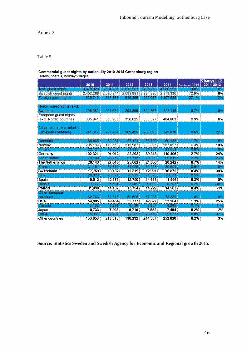
Inbound Tourism Modelling, Gothenburg Case
46
Annex 2
Table 5
Source: Statistics Sweden and Swedish Agency for Economic and Regional growth 2015.

Inbound Tourism Modelling, Gothenburg Case
47
Annex 3
Autocorrelation tests by Market.
Origin country; USA
Breusch-Godfrey LM test for autocorrelation
---------------------------------------------------------------------------
lags(p) | chi2 df Prob > chi2
-------------+-------------------------------------------------------------
1 | 1.398 1 0.2370
---------------------------------------------------------------------------
H0: no serial correlation
Origin country; Germany
Breusch-Godfrey LM test for autocorrelation
---------------------------------------------------------------------------
lags(p) | chi2 df Prob > chi2
-------------+-------------------------------------------------------------
1 | 6.615 1 0.0101
---------------------------------------------------------------------------
H0: no serial correlation
Origin country; United Kingdom
Breusch-Godfrey LM test for autocorrelation
---------------------------------------------------------------------------
lags(p) | chi2 df Prob > chi2
-------------+-------------------------------------------------------------
1 | 11.777 1 0.0006
---------------------------------------------------------------------------
H0: no serial correlation

Inbound Tourism Modelling, Gothenburg Case
48
Origin country; Norway
Breusch-Godfrey LM test for autocorrelation
---------------------------------------------------------------------------
lags(p) | chi2 df Prob > chi2
-------------+-------------------------------------------------------------
1 | 3.045 1 0.0810
---------------------------------------------------------------------------
H0: no serial correlation
Origin country; Domestic demand Sweden
Breusch-Godfrey LM test for autocorrelation
---------------------------------------------------------------------------
lags(p) | chi2 df Prob > chi2
-------------+-------------------------------------------------------------
1 | 12.081 1 0.0005
---------------------------------------------------------------------------
H0: no serial correlation

Inbound Tourism Modelling, Gothenburg Case
49
Annex 4
Table 6 Correlation between variables used in the estimation model ADLM
Norway GDPnw Prswnw Germany GDPge Prswge UK GDPuk Prswuk
Norway 1 GDPnw 0.0711 1
Prswnw -0.1296 0.0683 1 Germany 0.8779 0.6941 -0.023 1
GDPge 0.6297 0.9572 0.0862 0.6461 1 Prswge -0.0807 -0.1185 0.5472 0.1026 -0.1649 1
UK 0.8468 0.5895 0.0231 0.8247 0.5602 0.0471 1 GDPuk 0.8502 0.9248 0.0735 0.7906 0.8837 -0.0916 0.806 1
Prswuk -0.2847 -0.36 0.6032 -0.1617 -0.4242 0.7636 -0.1459 -0.3593 1 USA 0.8742 0.628 0.0373 0.8266 0.5295 0.1123 0.907 0.8089 -0.0857
GDPus 0.8797 0.9582 -0.024 0.8115 0.8729 -0.1191 0.7201 0.9559 -0.3513 Prswus -0.1389 0.0395 0.5725 0.0192 0.0968 0.2866 -0.0031 -0.0654 0.551 Sweden 0.8499 0.9709 -0.0289 0.7744 0.8932 -0.1355 0.6407 0.9217 -0.3747 GDPsw 0.7107 0.9876 0.0782 0.6689 0.9681 -0.1227 0.5746 0.9236 -0.4161
USA GDPus Prswus Sweden GDPsw USA 1
GDPus 0.7811 1 Prswus -0.0548 -0.0604 1
Sweden 0.7112 0.9882 -0.0413 1 GDPsw 0.5906 0.9302 -0.0079 0.9436 1

Inbound Tourism Modelling, Gothenburg Case
50
Annex 5
corrgram Norway
-1 0 1 -1 0 1
LAG AC PAC Q Prob>Q [Autocorrelation] [Partial Autocor]
-------------------------------------------------------------------------------
1 0.4671 0.4865 7.657 0.0057 |--- |---
2 0.3896 0.1960 13.162 0.0014 |--- |-
3 0.3062 -0.0292 16.68 0.0008 |-- |
4 0.0966 -0.1919 17.042 0.0019 | -|
5 0.0379 0.1264 17.1 0.0043 | |-
6 -0.0310 0.0049 17.14 0.0088 | |
7 -0.0406 0.1801 17.212 0.0161 | |-
8 -0.1008 -0.0179 17.673 0.0238 | |
9 -0.1483 -0.0531 18.713 0.0278 -| |
10 -0.1764 0.0280 20.251 0.0270 -| |
11 -0.2209 0.0415 22.78 0.0190 -| |
12 -0.2372 -0.0058 25.841 0.0113 -| |
13 -0.2335 0.0029 28.962 0.0066 -| |
14 -0.1762 0.1966 30.84 0.0058 -| |-
. corrgram Prnw
-1 0 1 -1 0 1
LAG AC PAC Q Prob>Q [Autocorrelation] [Partial Autocor]
-------------------------------------------------------------------------------
1 0.6191 0.6230 13.45 0.0002 |---- |----
2 0.4422 0.1161 20.541 0.0000 |--- |
3 0.3721 0.0538 25.736 0.0000 |-- |
4 0.3960 0.2023 31.828 0.0000 |--- |-
5 0.4228 0.4261 39.032 0.0000 |--- |---
6 0.2301 -0.0602 41.247 0.0000 |- |
7 0.1079 0.0762 41.754 0.0000 | |
8 0.0921 0.2289 42.139 0.0000 | |-

Inbound Tourism Modelling, Gothenburg Case
51
9 -0.0023 0.0617 42.139 0.0000 | |
10 -0.0573 -0.0054 42.301 0.0000 | |
11 -0.0893 0.1451 42.714 0.0000 | |-
12 -0.1465 -0.1025 43.882 0.0000 -| |
13 -0.0957 0.3512 44.406 0.0000 | |--
14 -0.1794 -0.2262 46.351 0.0000 -| -|
. corrgram Prswnw
-1 0 1 -1 0 1
LAG AC PAC Q Prob>Q [Autocorrelation] [Partial Autocor]
-------------------------------------------------------------------------------
1 0.3847 0.4051 5.1932 0.0227 |--- |---
2 -0.0455 -0.2584 5.2682 0.0718 | --|
3 0.0502 0.2042 5.3626 0.1471 | |-
4 0.1407 0.0731 6.132 0.1895 |- |
5 -0.0037 -0.1215 6.1325 0.2935 | |
6 -0.2244 -0.2610 8.239 0.2211 -| --|
7 -0.2166 -0.1317 10.28 0.1733 -| -|
8 -0.1763 -0.0359 11.689 0.1656 -| |
9 -0.0959 -0.0136 12.124 0.2064 | |
10 -0.0593 -0.0751 12.298 0.2656 | |
11 -0.0256 0.1607 12.332 0.3392 | |-
12 0.0118 -0.0408 12.339 0.4188 | |
13 0.0125 0.0162 12.348 0.4993 | |
14 -0.0237 -0.1791 12.382 0.5756 | -|

Inbound Tourism Modelling, Gothenburg Case
52
. corrgram GDPnw
-1 0 1 -1 0 1
LAG AC PAC Q Prob>Q [Autocorrelation] [Partial Autocor]
-------------------------------------------------------------------------------
1 0.8926 1.0437 27.963 0.0000 |------- |--------
2 0.7801 0.0926 50.032 0.0000 |------ |
3 0.6674 0.3898 66.742 0.0000 |----- |---
4 0.5708 -0.1850 79.403 0.0000 |---- -|
5 0.4850 -0.0295 88.882 0.0000 |--- |
6 0.3566 0.4279 94.203 0.0000 |-- |---
7 0.2496 1.3359 96.915 0.0000 |- |--------
8 0.1603 0.9117 98.08 0.0000 |- |-------
9 0.0818 -0.1089 98.396 0.0000 | |
10 0.0184 0.8676 98.413 0.0000 | |------
11 -0.0297 0.6159 98.459 0.0000 | |----
12 -0.0703 -0.6403 98.728 0.0000 | -----|
13 -0.1044 0.4343 99.352 0.0000 | |---
14 -0.1339 1.9132 100.44 0.0000 -| |--------
. corrgram Sweden
-1 0 1 -1 0 1
LAG AC PAC Q Prob>Q [Autocorrelation] [Partial Autocor]
-------------------------------------------------------------------------------
1 0.8841 1.0428 27.434 0.0000 |------- |--------
2 0.7678 -0.1946 48.812 0.0000 |------ -|
3 0.6634 0.0584 65.321 0.0000 |----- |
4 0.5724 0.1550 78.053 0.0000 |---- |-
5 0.4862 0.1871 87.581 0.0000 |--- |-
6 0.4076 0.2015 94.533 0.0000 |--- |-
7 0.3348 0.3407 99.411 0.0000 |-- |--
8 0.2636 0.0748 102.56 0.0000 |-- |
9 0.1846 0.2223 104.17 0.0000 |- |-

Inbound Tourism Modelling, Gothenburg Case
53
10 0.1132 -0.0960 104.81 0.0000 | |
11 0.0239 0.0247 104.84 0.0000 | |
12 -0.0573 0.0053 105.01 0.0000 | |
13 -0.1119 0.3048 105.73 0.0000 | |--
14 -0.1587 0.2592 107.25 0.0000 -| |--
. corrgram Prsw
-1 0 1 -1 0 1
LAG AC PAC Q Prob>Q [Autocorrelation] [Partial Autocor]
-------------------------------------------------------------------------------
1 0.7135 0.7399 17.868 0.0000 |----- |-----
2 0.5007 0.0030 26.96 0.0000 |---- |
3 0.4094 0.1364 33.249 0.0000 |--- |-
4 0.2972 -0.0390 36.681 0.0000 |-- |
5 0.2670 0.1755 39.554 0.0000 |-- |-
6 0.2681 0.0659 42.561 0.0000 |-- |
7 0.2338 0.1250 44.941 0.0000 |- |
8 0.2078 0.1398 46.898 0.0000 |- |-
9 0.0552 0.0364 47.042 0.0000 | |
10 -0.0818 0.0630 47.373 0.0000 | |
11 -0.0828 0.0666 47.728 0.0000 | |
12 -0.1298 0.0654 48.645 0.0000 -| |
13 -0.1629 -0.0102 50.165 0.0000 -| |
14 -0.2441 -0.1541 53.766 0.0000 -| -|

Inbound Tourism Modelling, Gothenburg Case
54
. corrgram GDPsw
-1 0 1 -1 0 1
LAG AC PAC Q Prob>Q [Autocorrelation] [Partial Autocor]
-------------------------------------------------------------------------------
1 0.8676 1.0039 26.42 0.0000 |------ |--------
2 0.7376 -0.0039 46.149 0.0000 |----- |
3 0.6115 0.4278 60.177 0.0000 |---- |---
4 0.5062 -0.1360 70.135 0.0000 |---- -|
5 0.4166 -0.0974 77.129 0.0000 |--- |
6 0.2971 0.5187 80.822 0.0000 |-- |----
7 0.2032 0.2807 82.62 0.0000 |- |--
8 0.1356 0.2323 83.453 0.0000 |- |-
9 0.0716 -0.2760 83.695 0.0000 | --|
10 0.0079 0.1415 83.698 0.0000 | |-
11 -0.0220 0.3769 83.723 0.0000 | |---
12 -0.0407 0.4276 83.814 0.0000 | |---
13 -0.0546 -0.0285 83.984 0.0000 | |
14 -0.0641 0.7740 84.233 0.0000 | |------
. corrgram Prnwsw
-1 0 1 -1 0 1
LAG AC PAC Q Prob>Q [Autocorrelation] [Partial Autocor]
-------------------------------------------------------------------------------
1 -0.0510 -0.3702 .09132 0.7625 | --|
2 -0.0119 -0.2312 .09648 0.9529 | -|
3 -0.0326 -0.4245 .13635 0.9871 | ---|
4 0.0959 0.6869 .49398 0.9741 | |-----
5 -0.0097 0.2520 .49778 0.9922 | |--
6 0.0010 0.3319 .49783 0.9979 | |--
7 -0.0379 -0.0913 .56031 0.9992 | |
8 -0.0604 -0.6344 .72569 0.9995 | -----|
9 -0.0156 -0.5482 .73723 0.9998 | ----|

Inbound Tourism Modelling, Gothenburg Case
55
10 -0.0320 -0.7523 .78794 0.9999 | ------|
11 0.0206 -0.2017 .80991 1.0000 | -|
12 -0.0449 -0.4173 .91937 1.0000 | ---|
13 -0.0495 -0.9497 1.0595 1.0000 | -------|
14 -0.0930 -2.2565 1.5827 1.0000 | --------|
. corrgram Germany
-1 0 1 -1 0 1
LAG AC PAC Q Prob>Q [Autocorrelation] [Partial Autocor]
-------------------------------------------------------------------------------
1 0.7524 0.7710 19.87 0.0000 |------ |------
2 0.5845 0.2476 32.261 0.0000 |---- |-
3 0.4403 -0.0717 39.534 0.0000 |--- |
4 0.3669 0.2113 44.766 0.0000 |-- |-
5 0.3355 0.0456 49.301 0.0000 |-- |
6 0.3269 0.1898 53.773 0.0000 |-- |-
7 0.3475 0.1631 59.028 0.0000 |-- |-
8 0.2903 0.0461 62.849 0.0000 |-- |
9 0.1925 0.0044 64.602 0.0000 |- |
10 0.0717 0.0026 64.856 0.0000 | |
11 -0.0140 -0.0444 64.866 0.0000 | |
12 -0.0598 -0.0832 65.061 0.0000 | |
13 -0.1080 -0.0609 65.729 0.0000 | |
14 -0.0915 0.2397 66.234 0.0000 | |-

Inbound Tourism Modelling, Gothenburg Case
56
. corrgram Prswge
-1 0 1 -1 0 1
LAG AC PAC Q Prob>Q [Autocorrelation] [Partial Autocor]
-------------------------------------------------------------------------------
1 -0.0179 -0.0195 .00804 0.9286 | |
2 -0.2620 -0.2799 1.8206 0.4024 --| --|
3 -0.1432 -0.1832 2.3908 0.4953 -| -|
4 0.1515 0.0915 3.0643 0.5471 |- |
5 -0.0349 -0.2224 3.102 0.6843 | -|
6 -0.2376 -0.7031 4.9655 0.5483 -| -----|
7 -0.0660 -0.0583 5.1187 0.6455 | |
8 0.1763 0.3489 6.2905 0.6147 |- |--
9 0.0614 -0.8361 6.4435 0.6948 | ------|
. corrgram GDPge
-1 0 1 -1 0 1
LAG AC PAC Q Prob>Q [Autocorrelation] [Partial Autocor]
-------------------------------------------------------------------------------
1 0.8906 0.9732 27.84 0.0000 |------- |-------
2 0.7779 -0.0913 49.786 0.0000 |------ |
3 0.6515 0.2371 65.708 0.0000 |----- |-
4 0.5267 -0.2782 76.487 0.0000 |---- --|
5 0.4019 -0.0272 82.997 0.0000 |--- |
6 0.2692 0.1017 86.031 0.0000 |-- |
7 0.1667 0.4306 87.24 0.0000 |- |---
8 0.0934 0.5724 87.636 0.0000 | |----
9 0.0408 0.0761 87.714 0.0000 | |
10 -0.0136 -0.2707 87.723 0.0000 | --|
11 -0.0303 0.1804 87.771 0.0000 | |-
12 -0.0221 0.7421 87.798 0.0000 | |-----
13 -0.0154 0.1469 87.811 0.0000 | |-
14 0.0008 -0.5221 87.811 0.0000 | ----|
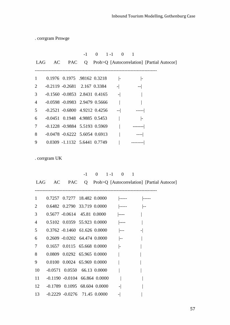
Inbound Tourism Modelling, Gothenburg Case
57
. corrgram Prnwge
-1 0 1 -1 0 1
LAG AC PAC Q Prob>Q [Autocorrelation] [Partial Autocor]
-------------------------------------------------------------------------------
1 0.1976 0.1975 .98162 0.3218 |- |-
2 -0.2119 -0.2681 2.167 0.3384 -| --|
3 -0.1560 -0.0853 2.8431 0.4165 -| |
4 -0.0598 -0.0983 2.9479 0.5666 | |
5 -0.2521 -0.6800 4.9212 0.4256 --| -----|
6 -0.0451 0.1948 4.9885 0.5453 | |-
7 -0.1228 -0.9884 5.5193 0.5969 | -------|
8 -0.0478 -0.6222 5.6054 0.6913 | ----|
9 0.0309 -1.1132 5.6441 0.7749 | --------|
. corrgram UK
-1 0 1 -1 0 1
LAG AC PAC Q Prob>Q [Autocorrelation] [Partial Autocor]
-------------------------------------------------------------------------------
1 0.7257 0.7277 18.482 0.0000 |----- |-----
2 0.6482 0.2790 33.719 0.0000 |----- |--
3 0.5677 -0.0614 45.81 0.0000 |---- |
4 0.5102 0.0359 55.923 0.0000 |---- |
5 0.3762 -0.1460 61.626 0.0000 |--- -|
6 0.2609 -0.0202 64.474 0.0000 |-- |
7 0.1657 0.0115 65.668 0.0000 |- |
8 0.0809 0.0292 65.965 0.0000 | |
9 0.0100 0.0024 65.969 0.0000 | |
10 -0.0571 0.0550 66.13 0.0000 | |
11 -0.1190 -0.0104 66.864 0.0000 | |
12 -0.1789 0.1095 68.604 0.0000 -| |
13 -0.2229 -0.0276 71.45 0.0000 -| |

Inbound Tourism Modelling, Gothenburg Case
58
. corrgram Prswuk
-1 0 1 -1 0 1
LAG AC PAC Q Prob>Q [Autocorrelation] [Partial Autocor]
-------------------------------------------------------------------------------
1 0.4645 0.5046 6.0693 0.0138 |--- |----
2 0.1124 -0.1008 6.4403 0.0399 | |
3 -0.0747 -0.1007 6.6116 0.0854 | |
4 -0.0630 0.0667 6.7391 0.1503 | |
5 -0.1720 -0.1071 7.7374 0.1713 -| |
6 -0.0946 -0.0118 8.0555 0.2341 | |
7 -0.0062 0.0784 8.0569 0.3276 | |
8 0.0283 -0.0798 8.0887 0.4249 | |
9 -0.0296 -0.1154 8.1257 0.5215 | |
10 0.0361 0.5789 8.1843 0.6108 | |----
. corrgram GDPuk
-1 0 1 -1 0 1
LAG AC PAC Q Prob>Q [Autocorrelation] [Partial Autocor]
-------------------------------------------------------------------------------
1 0.9154 0.9840 29.413 0.0000 |------- |-------
2 0.8159 -0.2616 53.555 0.0000 |------ --|
3 0.7192 0.3617 72.962 0.0000 |----- |--
4 0.6284 -0.2166 88.304 0.0000 |----- -|
5 0.5433 0.2547 100.2 0.0000 |---- |--
6 0.4406 0.6711 108.32 0.0000 |--- |-----
7 0.3356 0.7235 113.22 0.0000 |-- |-----
8 0.2445 0.1891 115.93 0.0000 |- |-
9 0.1596 -0.3378 117.14 0.0000 |- --|
10 0.0730 0.0091 117.4 0.0000 | |
11 0.0037 0.4641 117.4 0.0000 | |---
12 -0.0562 1.2978 117.58 0.0000 | |--------
13 -0.1048 0.2161 118.2 0.0000 | |-

Inbound Tourism Modelling, Gothenburg Case
59
. corrgram Prnwuk
-1 0 1 -1 0 1
LAG AC PAC Q Prob>Q [Autocorrelation] [Partial Autocor]
-------------------------------------------------------------------------------
1 0.4264 0.4264 5.1128 0.0238 |--- |---
2 0.2372 0.0727 6.7635 0.0340 |- |
3 0.2248 0.1380 8.3145 0.0399 |- |-
4 -0.2033 -0.4679 9.6432 0.0469 -| ---|
5 -0.0784 0.1641 9.8509 0.0796 | |-
6 -0.1248 -0.1824 10.404 0.1086 | -|
7 -0.2439 0.0093 12.635 0.0815 -| |
8 -0.1232 -0.3269 13.237 0.1039 | --|
9 -0.2477 -0.1986 15.825 0.0706 -| -|
10 -0.2469 -0.3608 18.568 0.0461 -| --|
. corrgram USA
-1 0 1 -1 0 1
LAG AC PAC Q Prob>Q [Autocorrelation] [Partial Autocor]
-------------------------------------------------------------------------------
1 0.5412 0.5413 10.28 0.0013 |---- |----
2 0.4010 0.2012 16.111 0.0003 |--- |-
3 0.5482 0.3636 27.385 0.0000 |---- |--
4 0.4582 -0.0386 35.543 0.0000 |--- |
5 0.2961 -0.2768 39.076 0.0000 |-- --|
6 0.2380 -0.1295 41.446 0.0000 |- -|
7 0.1328 -0.1014 42.213 0.0000 |- |
8 0.1017 0.0063 42.683 0.0000 | |
9 0.0255 0.0624 42.713 0.0000 | |
10 -0.0488 -0.0040 42.831 0.0000 | |
11 -0.1284 0.0640 43.686 0.0000 -| |
12 -0.2099 -0.1058 46.082 0.0000 -| |
13 -0.1804 0.2409 47.945 0.0000 -| |-

Inbound Tourism Modelling, Gothenburg Case
60
. corrgram GDPus
-1 0 1 -1 0 1
LAG AC PAC Q Prob>Q [Autocorrelation] [Partial Autocor]
-------------------------------------------------------------------------------
1 0.9099 1.0167 29.056 0.0000 |------- |--------
2 0.8198 -0.3883 53.431 0.0000 |------ ---|
3 0.7331 0.2760 73.595 0.0000 |----- |--
4 0.6484 0.2517 89.932 0.0000 |----- |--
5 0.5652 0.1559 102.81 0.0000 |---- |-
6 0.4716 0.2224 112.11 0.0000 |--- |-
7 0.3756 -0.6080 118.25 0.0000 |--- ----|
8 0.2828 -0.5444 121.87 0.0000 |-- ----|
9 0.1950 -0.3689 123.67 0.0000 |- --|
10 0.1127 1.0021 124.3 0.0000 | |--------
11 0.0376 -1.1706 124.37 0.0000 | --------|
12 -0.0333 0.7446 124.43 0.0000 | |-----
13 -0.1012 1.5894 125.02 0.0000 | |--------
14 -0.1669 0.0459 126.7 0.0000 -| |
. corrgram Prswus
-1 0 1 -1 0 1
LAG AC PAC Q Prob>Q [Autocorrelation] [Partial Autocor]
-------------------------------------------------------------------------------
1 0.6661 0.7106 15.571 0.0001 |----- |-----
2 0.5397 0.2512 26.133 0.0000 |---- |--
3 0.4371 0.0116 33.301 0.0000 |--- |
4 0.3141 -0.0575 37.133 0.0000 |-- |
5 0.3012 0.1933 40.789 0.0000 |-- |-
6 0.1948 -0.1454 42.377 0.0000 |- -|
7 0.2206 0.2270 44.495 0.0000 |- |-
8 0.1627 0.1112 45.695 0.0000 |- |
9 -0.0150 -0.2110 45.706 0.0000 | -|

Inbound Tourism Modelling, Gothenburg Case
61
10 -0.1401 -0.0555 46.677 0.0000 -| |
11 -0.1828 -0.0123 48.409 0.0000 -| |
12 -0.1817 0.0684 50.205 0.0000 -| |
13 -0.2656 -0.2687 54.244 0.0000 --| --|
14 -0.2819 -0.1709 59.046 0.0000 --| -|
. corrgram Prnwus
-1 0 1 -1 0 1
LAG AC PAC Q Prob>Q [Autocorrelation] [Partial Autocor]
-------------------------------------------------------------------------------
1 0.0026 0.0022 .00023 0.9879 | |
2 0.1604 0.1622 .93366 0.6270 |- |-
3 0.1391 0.1500 1.6595 0.6460 |- |-
4 0.0258 0.0054 1.6853 0.7934 | |
5 0.1142 0.8302 2.2108 0.8193 | |------
6 -0.0256 -0.3274 2.2382 0.8965 | --|
7 0.0090 0.2898 2.2417 0.9453 | |--
8 -0.0127 -0.0550 2.2491 0.9724 | |
9 -0.0009 0.3426 2.2491 0.9869 | |--
10 -0.0112 -0.0146 2.2554 0.9940 | |
11 -0.0327 0.3364 2.3108 0.9971 | |--
12 -0.0049 0.6100 2.3122 0.9988 | |----
13 0.0370 0.8536 2.3904 0.9994 | |------
14 -0.0235 0.0245 2.4239 0.9997 | |