Inattentive Importers ∗

KUNAL DASGUPTA † JORDI MONDRIA ‡

PRELIMINARY AND INCOMPLETE

Abstract

Importers rarely observe the price of every good in every market because of information

frictions. In this paper, we aim to explain how the presence of such frictions shape the pattern

of trade across countries. To this end, we introduce rationally inattentive importers in a multi-

country, multi-good Ricardian trade model. We derive a gravity-like equation linking bilateral

trade flows and the cost of processing information faced by importers. In this setting, a

reduction in conventional trade costs has large effects on trade flows as importers re-optimize

information processing across countries. The model explains a number of findings in the

literature related to the response of trade flows to various trade barriers.

∗We would like to thank Victor Aguirregabiria, Martin Burda, Davin Chor, Arnaud Costinot, Michal Fabinger,Peter Morrow, Ananth Ramanarayanan and Kim Ruhl for helpful discussion.†University of Toronto.‡University of Toronto.

1 Introduction

Trade costs are high. Our understanding of the determinants of these costs, however, remainslimited (Head and Mayer, 2013). One possible source of such costs is information frictions.Imperfect information about prices plagues markets. An importer rarely observes the price of agiven product in every market. How does imperfect information affect international trade flows?In this paper, we take a first step towards answering this question.

Despite a widespread agreement among economists that imperfect information could and docreate significant barriers to trade, we lack a framework that formalizes the link between informa-tion and trade. The difficulty in developing such a framework is due to the absence of a standardway of modeling information. In the international trade literature, the informational structure isusually treated as exogenous. But as Anderson and van Wincoop (2004) point out in their defini-tive survey on trade costs, we need more careful modeling of information costs. We believe thatby treating information as a parameter that is determined outside the model, we are missing outon several interesting insights, some of which could have potentially important implications forhow countries trade. Borrowing tools from the rational inattention literature (Sims, 2003, 2006),we develop a model of information and trade.

Our decision to model information as in the rational inattention theory is guided by three con-siderations. First, the central premise of this theory is that although information is freely available,agents have a limited capacity to process information. Faced with a capacity constraint, agentsmust decide how much information they want to process about their variable(s) of interest. Webelieve this to be a quite accurate description of the real world. Second, rational inattention hasan appealing feature that the process through which agents process information is endogenous.In the context of our model, this causes importers to have a different level of information aboutdifferent source countries in equilibrium, without taking recourse to ad-hoc differences in suchinformation across countries. And finally, by using rational inattention, we can appeal to pow-erful results from the multinomial choice literature that allows us to derive elegant, closed-formsolutions for bilateral trade flows as functions of information costs and other primitives. Thisallows us to perform simple comparative static exercises, despite a complex underlying problem.

We introduce rational inattention in a N -country, multi-good Ricardian model of trade. Asin Eaton and Kortum (2002), we model productivity of a good as stochastic. The key object ofinterest in our model is the unconditional probability that importers in country j buy a good kfrom producers in country i, πij(k). Following Matejka and McKay (2012), we derive a systemof equations involving the πij(k)s, i = 1, ....N , for a particular j. Solving these unconditionalprobabilities requires solving N -dimensional integrals. We show that when the productivity dis-

1

tributions have a particular form, one can obtain closed-form solutions for the πij(k)s. Under amild condition, we obtain a gravity-like equation linking bilateral trade with the cost of processinginformation. We believe this to be one of the main contributions of the paper.

The endogenous processing of information affects the response of trade flows to a changein conventional trade frictions between trading partners. As the trade cost between importingcountry j and exporting country i declines, country j importers start to purchase more fromcountry i because the average price offered by country i producers is now lower. This is thestandard effect of trade costs on trade flows present in any trade model. In our model, there isan additional effect however. Faced with a cost of processing information, importers in countryj choose how much information to process about every source country, including country j. Alowering of expected price in country i raises the expected benefit of processing information aboutcountry i. Country j importers respond by paying more attention to country i and less attentionto every other country, thereby boosting the volume of trade between j and i further. Thus, whenimporters are rationally inattentive, small differences in conventional trade costs could have largeeffect on trade flows - there is a magnification effect. This is the key insight of our model ofinattentive importers. We show that this mechanism can explain a number of findings in theliterature related to the response of trade flows to various trade barriers.

A number of papers have provided evidence of informational asymmetry in internationaltrades. Using data on trade in agricultural goods in Philippines, Allen (2012) shows that mostof the reduction in trade can be attributed to informational frictions, thereby highlighting theirsignificance. In a highly influential paper, Rauch (1999) showed that proximity, common lan-guage and colonial ties are more important for trade in differentiated products, which is moredependent on information, than for products traded on organized exchanges. Gould (1994) showsthat immigrant links to the home country have a strong positive effect on both exports and importsfor the U.S. while Head and Ries (1998) find the same for Canada. Although higher import fromthe home country could simply reflect greater demand from the immigrants, the same cannot besaid of exports. The latter, the argument goes, probably reflects better information possessed bythe immigrants about their home markets. Rauch and Trindade (2002) find that for differentiatedgoods, the presence of ethnic Chinese networks in both the trading partners increases trade.

One of the few papers to explicitly use proxies for information cost in explaining trade flowsis Portes and Rey (2005). They run a standard gravity equation and find that informational flows,captured by telephone call traffic and multinational bank branches, have significant explanatorypower for bilateral trade flows. Morales et al. (2011) show that the entry of a exporter in a partic-ular market increases the likelihood of his entry into other similar markets. Their finding seems

2

to suggest that we may not be in a full information world, and when a firm enters a market, itgets new information about similar markets. An absence of perfect information about foreignmarkets also features in the exporting models of Eaton et al. (2010) and Albornoz et al. (2012).Chaney (2013) incorporates exporter networks into a model of trade. Among other things, heshows that his network model can explain the distribution of foreign markets accessed by individ-ual exporters. The importance of networks in trade is suggestive of the presence of informationalbarriers.

The paper that is closest in spirit to our paper is Allen (2012). He considers producers se-quentially searching for the lowest price across markets which makes information about pricesendogenous. As in our paper, Allen derives bilateral trade flows as a function of informationcosts. Our model, however, differs from Allen (2012) in two important ways. First, the infor-mation friction in our model is on the side of the buyers, rather than sellers. Producers in Allen(2012) search for the most attractive market while importers in our model search for the mostattractive source. Second, in Allen (2012) if a producer searches N markets, he exactly knowsthe price in those N markets and has no information about prices in the remaining markets. Incontrast, importers in our model have varying degrees of information about every market, butnever observe prices in any market perfectly.

In a related paper, Arkolakis et al. (2012) introduce staggered adjustment in the Eaton-Kortummodel of trade. They assume that in each period, consumers continue to buy from the samesupplier with some probability - consumers are inattentive. Accordingly, with some probability,consumers do not respond to price shocks that hit other suppliers. Arkolakis et al. takes theinattention as given, however, and is therefore silent on how the degree of inattention itself couldrespond to trade costs.

Recent work in the areas of macroeconomics and finance has used information theoretic ideas.In macroeconomics, Sims (2003, 2006), Luo (2008), Luo and Young (2009) and Tutino (2013)have applied rational inattention to study the consumption and savings behavior of households.Mackowiak and Wiederholt (2009), Woodford (2009) and Matejka (2012) have used informationtheoretic ideas to analyze the price setting behavior of firms. In finance, Peng and Xiong (2006),Van Nieuwerburgh and Veldkamp (2009, 2010) and Mondria (2010) have applied rational inat-tention in asset pricing and portfolio choice models. To the best of our knowledge, we are the firstones to apply rational inattention to the study of international trade.

The rest of the paper is organized as follows. In Section 2, we specify preferences, produc-tion structure and the market clearing conditions. Section 3 introduces inattentive importers andderives the equilibrium. We also perform meaningful comparative statics in this section, for a

3

given distribution of wages and input costs across countries. In Section 4, we numerically solvethe full general equilibrium of the model and perform counterfactuals. Section 5 concludes. Allthe proofs are in the Appendix.

2 Model

We consider a Ricardian model of trade with N countries. Country i is populated by Li indi-viduals. Each individual consumes a final good and supplies a unit of labor inelastically. Forsimplicity, we assume that labor is the only factor of production. Labor is perfectly mobile withina country but immobile across countries. There are two sectors that add value domestically - anintermediate goods sector that produces intermediate inputs that can be traded, and a final goodssector that produces a non-traded good for consumption. Henceforth, we shall express all thevariables in per capita terms.

Trade costs. The “standard” trade cost between exporting country i and importing country j iscaptured by τij . We do not take a stand on the interpretation of τij (i.e., whether it is an icebergcost) until later, except noting that a higher value corresponds to higher trade costs. τij includes alltypes of costs that are typically suggested by the gravity literature like transportation costs, bordercosts, policy barriers, etc. Importantly, this does not include information costs. For simplicity, weassume that trade costs are symmetric.

Intermediate good sector. There is a continuum of intermediate inputs indexed by k ∈ [0, 1].Production of each intermediate requires labor and an aggregate of all the intermediates. Good kcan be produced in country i and made available to country j using the following technology:

qij(k) = f(li, Qi, Ai, z(k),

1

τij

),

where li and Qi denotes the amount of labor and the aggregate intermediate good. Ai is a locationparameter common to all goods k produced in country i, while z(k) is a random shock drawnindependently for each good k from a cumulative distribution function F (z), with a zero locationparameter, which is assumed to be common across countries.1 We separate the location parameter,Ai, from the random productivity realizations for tractability reasons. At this point we simplyassume that f ′ is positive with respect to each of its arguments. We shall have more to say aboutthe functional form for f later on.

1All the results in the paper are robust to making Ai good-specific and z(k) country-specific.

4

Each intermediate good is combined using a CES aggregator into Qi:

Qi = [

∫ 1

0

qi(k)1− 1σ dk]

σσ−1 ,

where σ > 1 is the elasticity of substitution. The CES aggregate is produced by competitive firmssimply by combining all the intermediates. The producers of the aggregate good (henceforthimporters) in country i purchase intermediate goods from all over the world; the correspondingamounts are given by qi(k). The price of one unit of the aggregate is then given by

Pi = [

∫ 1

0

pi(k)1−σdk]1

σ−1 , (1)

where pi(k) is the price of good k paid by importers in country i.

Final good sector. Perfectly competitive firms combine labor and intermediate goods to producea final good:

yi =( liα

)α( Qi

1− α

)1−α.

We assume that yi is also the utility of each individual in country i. The share of labor in finalgood production, α, is common across countries. The price of the final good is then

si = wαi P1−αi , (2)

where wi is the wage in country i.

Cost of intermediates. The cost of importing one unit of good k from country i to country j isgiven by 1/zij(k), where zij(k) is the adjusted productivity of country i (adjusted for trade costs).In this paper, we use two alternative definitions of zij(k):

ASSUMPTION 1A: zij(k) = Ai+z(k)

(wβi P1−βi )τij

.

ASSUMPTION 1B: zij(k) = Ai(wβi P

1−βi )τij

+ z(k).

Under Assumption 1A, trade costs and input costs in country i affect both the location pa-rameter and the shape of the productivity distribution in country i in producing good k forcountry j, as in Eaton and Kortum (2002). Such importing costs costs can be generated iff = C[Ai + zi(k)]lβi Q

1−βi /τij , where C is some constant. Under this assumption, our model

cannot be solved analytically. But because this is the more standard assumption in the literature,

5

we study the properties of the model under this assumption numerically.Under assumption 1B, trade costs and input costs only affect the location parameter in country

i. This assumption has two advantages. First, this specification for costs allows us to obtain aclosed-form solution for trade shares and gain intuition about the new friction introduced in thepaper. Second, this specification introduces a smaller error when computing trade flows if the truetrade costs are of a per unit nature rather than ad-valorem.2

Importers in j want to pay the lowest price for each good k. They would ideally like to importgood k from the most efficient country, that is the country with max[zij(k); i = 1, ..., N ]. Pricesand productivity realizations, however, are not perfectly observed when importers choose thecountry from where to purchase the good. We assume though, that the price of good k in countryi becomes fully observable once country i has been chosen to supply a good. This assumption ofperfect observability ex-post, combined with perfect competition in the market for intermediateinputs, implies that the producers of the same intermediate good in any country do not engage instrategic price setting.3 The price at which producers in country i are willing to sell good k toimporters in country j is then given by

pij(k) =1

zij(k). (3)

i.e., producers are willing to sell their goods at marginal cost. It must be emphasized that pij(k)

is the price that is actually paid by country j importers if they choose to purchase good k fromcountry i. The un-observability of prices ex-ante, however, implies that pij(k) may not be thelowest price for good k faced by the importers in country j.

Market clearing. Let the set of intermediate goods that country j purchases from country i bedenoted by Ωij ⊂ [0, 1]. The share of expenditure by country j on goods imported from countryi is given by

sij =

∫Ωij

pij(k)qij(k)dk/(LjPjQj),

where LjPjQj is the total expenditure on intermediates in country j. The total imports in country

2To see this, suppose the true cost of intermediate good k produced by country i in country j is 1zi+z(k) + τij ,

where τij > 0. This can be re-written as [1 + τij ]1

zi+z(k) , where τij = τij(zi + z(k)). The ad-valorem trade costis increasing in productivity. Hence, if we use an ad-valorem cost that is invariant across source countries, we endup predicting more trade with less productive source countries and less trade with more productive source countriesrelative to what the data might suggest. Under our assumption 1B, the error would still be there, but would be smallerbecause the ad-valorem cost is unaffected by z(k).

3Essentially, in the presence of information frictions, firms selling a homogeneous good might choose to chargea price greater than marginal cost even with free entry.

6

i are given byImports = LiPiQi

∑j 6=i

sji.

while total exports are given by

Exports =∑j 6=i

sijLjPjQj.

Balanced trade requires that

LiPiQi

N∑j=1

sji =N∑j=1

sijLjPjQj,

where exports and imports are now been broadly defined to include country i’s sale to itself.Following Alvarez and Lucas (2007), it can be shown that the trade balance equation reduces toa system of equations involving the wages:

Liwi =N∑j=1

sijLjwj. (4)

As we show in the next section, the sij-s are functions of wi and other parameters. Hence, giventhe endowment of labor in each country, (4) represents N non-linear equations in N unknowns -wi. As shown by Alvarez and Lucas (2007), this system of equations will typically have at leastone set of solution.

In the next section, we introduce inattentive importers and solve for the equilibrium of themodel. All the results in this section are conditional on wages and input prices.

3 Rationally Inattentive Importers

We assume that importers are rationally inattentive. Importers choose how to process informationabout each country, given a limited capacity to process information. In equilibrium, this yieldsthe amount of information they have about each country. The innovation provided by rationalinattention is that importers are not constrained to learn about each country’s productivity drawswith a particular signal structure, but rather, are allowed to choose the optimal mechanism toprocess information. As argued by Sims (2003) and Matejka and McKay (2012), there is no needto model the signal structure explicitly - it is enough to solve for the optimal joint distribution

7

of the variable of interest and actions. In our model, importers choose the (i) joint distributionof trade cost adjusted productivity in each country, and (ii) the country from where to import aparticular good, subject to a capacity constraint for processing information.

3.1 Information

Following Sims (2003), we use tools from information theory to model the limited informationprocessing capabilities of importers. We define λj(k) as the unit cost of information of country jimporters about good k and κj(k) as the total amount of information processed by country j aboutsuppliers of good k. Let Z(k) be the vector of adjusted productivity realizations of all countriesfor good k. Information theory measures information as the reduction in uncertainty. By payinga cost λj(k)κj(k), country j importers can reduce their uncertainty about the realization of Z(k)

by κj(k). We use entropy as the measure of uncertainty about Z(k) and mutual information asthe measure of uncertainty reduction.

Definition. The entropy H(X) of a discrete random variable X that takes values x in X is

H(X) = −∑x∈X

p(x) log p(x),

where p(x) is the probability mass function of X .

Definition. The mutual information of two random variables X and Y (taking values y in Y) isgiven by

I(X;Y ) =∑x∈X

∑y∈Y

p(x, y) logp(x, y)

p(x)p(y),

where p(x, y) is the joint probability mass function of X and Y , while p(y) is the marginal prob-ability mass function of Y .

In other words, entropy is the expectation of log( 1p(x)

). As an example, consider a randomvariable that takes only two values: x1 with probability p and x2 with probability 1 − p. Theentropy of this random variable is −p log p − (1 − p) log(1 − p). Figure 1 plots the entropy as afunction of p. As the figure suggests, entropy is a hump-shaped function, attaining a maximumat p = 1

2and a minimum of zero for both p = 0 and p = 1. These properties of entropy

are actually quite general. When p = 0, 1, the random variable is not “random” any more.Accordingly, there is no uncertainty - entropy is zero. But as p rises above zero (or falls below

8

one), uncertainty is introduced and consequently entropy becomes positive. Entropy is maximumwhen all realizations of p are equally likely.

0 0.2 0.4 0.6 0.8 10

0.1

0.2

0.3

0.4

0.5

0.6

0.7

p

Ent

ropy

Figure 1: Entropy when the random variable is binary

It is straight-forward to show that mutual information can be re-written as

I(X;Y ) = H(X)− Ey[H(X|Y )],

where H(X|Y ) = −∑

x p(x|y) log p(x|y) is the entropy of X conditional on Y . The followingproperties of mutual information (Cover and Thomas, 1991) will be useful later on:

PROPERTY 1: I(X;Y ) ≥ 0.

PROPERTY 2: H(X)− Ey[H(X|Y )] = H(Y )− Ex[H(Y |X)].

Because of Property 1, mutual information can be interpreted as the reduction in uncertaintyinX caused by the knowledge of Y . Property 2 suggests that the role ofX and Y in the definitioncan be reversed.

3.2 Results for the General Case

In our model, importers face uncertainty regarding which country has the highest adjusted pro-ductivity, and hence, the lowest cost of delivering good k. The object of interest is the likelihood

9

of importing a good from a particular country. Let us define fij(k) as the probability that country jbuys good k from country i conditional on the realization of Z(k), and πij(k) as the unconditionalprobability that country j buys good k from country i. Then,

πij(k) =

∫Z(k)

fij(k)dF (Z(k)). (5)

Importers in country j process information about Z(k) to reduce its entropy H(Z(k)). Insteadof explicitly modeling the optimal signal structure, rational inattention allows us to measure un-certainty reduction as the mutual information between Z(k) and the country i chosen by countryj:

κj(k) = H(Z(k)

)− Ei

[H(Z(k)|ij

)]= H(ij)− EZ(k)

[H(ij|Z(k)

)]= −

N∑i=1

πij(k) log πij(k) +

∫Z(k)

( N∑i=1

fij(k) log fij(k))dF (Z(k)).

(6)

where the equality between the first and the second line follows from Property 2. H(ij), in theabove equation, captures the ex-ante uncertainty of country j’s importers about which countryi to buy good k from. Once the importers observe Z(k), albeit imperfectly, their uncertaintyis reduced. The resulting difference is the information that country j importers have about theproductivity of exporters across the world in good k.

If information could be processed freely, an importer would find out the true realization ofZ(k). There are, however, a multitude of costs, captured by λj(k), involved in processing infor-mation about the true productivity of a supplier. Importers in country j choose to consume goodk from the country that has the highest expected productivity, taking into account the informationprocessing costs. Therefore, importers in country j solve the following optimization problem:

max[fij(k)]Ni=1

N∑i=1

∫Z(k)

zij(k)dF (Z(k))− λj(k)κj(k), (7)

10

subject to

fij(k) ≥ 0 ∀i, (8)N∑i=1

fij(k) = 1, (9)

where κj(k) is given by (6), fij(k) is given by (5) and 1/zij(k) is the trade cost adjusted price.Rationally inattentive importers choose a probability distribution over where to buy good k from.Following Matejka and McKay (2012), the next proposition derives the equilibrium conditionalprobabilities.

Proposition 1. If λj(k) > 0, then conditional on the realization of Z(k), the probability of

importers in country j choosing to import good k from country i ∈ 1, ..., N is given by

fij(k) =πij(k) exp

( zij(k)

λj(k)

)∑N

h=1 πhj(k) exp( zhj(k)

λj(k)

) . (10)

If the countries are a priori identical, then πij(k) = 1/N for all i and the posterior probabilitythat country j buys good k from country i follows a multinomial logit (REFERENCE). Hence,in this model, the demand for goods is a modified multinomial logit that takes into account thepriors, πij(k). The following corollary makes an important observation:

Corollary 1. If @i such that πij(k) = 1 and πhj(k) = 0 for all h 6= i, then @i such that fij(k) = 1.

If the importers in country j attach positive prior probabilities of importing good k from atleast two countries, then conditional on the productivity draws, they will never buy good k fromonly one country. Notice that the corollary contrasts sharply with the result in Eaton and Kortum(2002). In their paper, even though the prior (unconditional) probabilities of importing good kby country j is positive for every exporting country i, this probability drops to zero for everyexporting country but one after the productivity draws are realized. Under full information, oncethe productivities are drawn, importers in country j purchase good k almost surely from onecountry, the country which has the lowest cost of delivering good k to country j. In our model,this is not true any more. If country j is populated by a large number of importers for each good k,by applying a Law of Large Numbers we can conclude that a fraction fij(k) of them will import

11

the good from country i.4 In the literature, when a narrowly defined good is imported from manycountries, it is customary to assume that they represent different varieties (REFERENCE). In ourmodel, a good that is identical in every respect could still be imported from multiple countriesbecause of information frictions.

In the next few propositions, we characterize the unconditional probability that country j

chooses to import good k from country i.

Proposition 2. πij(k) is increasing in the location parameter Ai and decreasing in input costs

wi, Pi, and trade costs τij .

Proposition 2 states that a priori, importers in country j are less likely to purchase goodsfrom countries that are farther away or have higher input costs, other things remaining equal.A decrease in Ai lowers the the average productivity of good k in country i and reduces theprobability that the price of good k in i is the lowest expected price. In a full information model,this results in a lower probability of purchasing good k from country i. In our model, thereis an additional effect. The rationally inattentive importer in country j compares the expectedmarginal benefit of processing information about country i’s productivity with the marginal costof information. As the probability of getting a lower price in country i declines, so does theinformation processed by country j importers about country i. Consequently, πij(k) drops further- the presence of information costs creates a magnification effect. The same mechanism reducesπij(k) following an increase in input costs or trade costs.

Proposition 3. If countries are identical but τij > τjj for all i 6= j, πjj(k) is increasing in λj(k).

Proposition 3 states that all else equal, an increase in the cost of processing information in-creases the probability of purchasing good k from the home country. Intuitively, the higher arethe information processing costs, the less information importers are able to incorporate into theirdecision making and the greater is the weight attached to the initial priors. Because the expectedadjusted productivity in the home country is the highest among all the countries because of tradecosts, increased importance of the prior raises the likelihood of buying the good from the homecountry. This result is related to findings of home bias in consumption. DISCUSS THEIR FIND-INGS. It must be emphasized that the home bias in our model arises not due to exogenous dif-ferences in the information structure, but endogenous differences in information across countriesbeing processed by importers.

Proposition 4. If countries are identical but τij > τjj for all i 6= j, then as λj(k) → ∞,

πij(k)→ 0 for all i 6= j and πjj(j)→ 1.4Because of perfect competition among the importers, the number of importers is not determined.

12

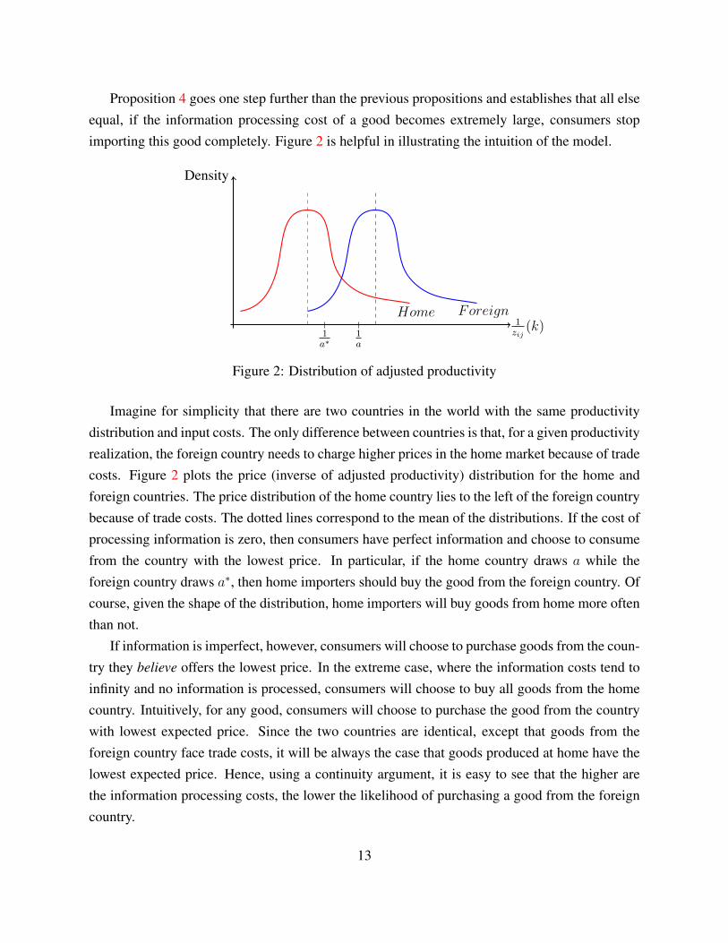
Proposition 4 goes one step further than the previous propositions and establishes that all elseequal, if the information processing cost of a good becomes extremely large, consumers stopimporting this good completely. Figure 2 is helpful in illustrating the intuition of the model.

Home Foreign

1a∗

1a

1zij

(k)

Density

Figure 2: Distribution of adjusted productivity

Imagine for simplicity that there are two countries in the world with the same productivitydistribution and input costs. The only difference between countries is that, for a given productivityrealization, the foreign country needs to charge higher prices in the home market because of tradecosts. Figure 2 plots the price (inverse of adjusted productivity) distribution for the home andforeign countries. The price distribution of the home country lies to the left of the foreign countrybecause of trade costs. The dotted lines correspond to the mean of the distributions. If the cost ofprocessing information is zero, then consumers have perfect information and choose to consumefrom the country with the lowest price. In particular, if the home country draws a while theforeign country draws a∗, then home importers should buy the good from the foreign country. Ofcourse, given the shape of the distribution, home importers will buy goods from home more oftenthan not.

If information is imperfect, however, consumers will choose to purchase goods from the coun-try they believe offers the lowest price. In the extreme case, where the information costs tend toinfinity and no information is processed, consumers will choose to buy all goods from the homecountry. Intuitively, for any good, consumers will choose to purchase the good from the countrywith lowest expected price. Since the two countries are identical, except that goods from theforeign country face trade costs, it will be always the case that goods produced at home have thelowest expected price. Hence, using a continuity argument, it is easy to see that the higher arethe information processing costs, the lower the likelihood of purchasing a good from the foreigncountry.

13

Observe that while deriving Propositions 1, 2, 3 and 4, we did not specify a particular func-tional form for zij(k) or for the distribution of random productivity draws F (z). In particular,these results are satisfied under both assumptions 1A and 1B and for any F (z). At this level ofgenerality, however, we cannot explicitly solve for the πij(k)-s. Rather, we have to solve for thefixed point of (5) where fij(k) is given by (10).

3.3 Closed-form solution for a particular F (z)

Here we use Assumption 1B and a specific form for F (z) to derive of a closed-form solutionfor πij(k). This facilitates a more detailed analysis of the model. Following Cardell (1997), wedefine a distribution C(λ).

Definition. For 0 < λ < 1, C(λ) is a distribution with a probability density function given by

gλ(z) =1

λ

∞∑n=0

[(−1)ne−nz

n!Γ(−λn)

](11)

−10 −5 0 5 100

0.05

0.1

0.15

0.2

0.25

0.3

0.35

0.4

0.45

0.5

z

g λ(z)

C(λ)Gumbel

Figure 3: Distribution C(λ)

The main property of the C(λ) distribution is that if a random variable ε is drawn from a TypeI extreme value (Gumbel) distribution and another random variable ν is drawn from C(λ), thenν + λε is a random variable distributed as Type I extreme value. The relation between C(λ) and

14

a Gumbel distribution is shown in Figure 3.5 It is clear that qualitatively, the two distributions arevery similar. The next proposition shows that when Assumption 1B is satisfied and the randomproductivities are drawn from a C(λ) distribution, there exists a closed-form solution for πij(k).

Proposition 5. Under assumption 1B, if the z(k)-s are drawn independently from a cumulative

distribution C(λ(k)

)where 0 < λ(k) < 1, then πij(k) is given by

πij(k) =exp

( zij1−λ(k)

)∑Nh=1 exp

( zhj1−λ(k)

) ,where zij = Ai

(wβi P1−βi )τij

.

The unconditional probability that country j buys good k from country i follows a multino-mial logit. This result contributes to the literature on rational inattention by finding a closed-formsolution to a problem with asymmetric prior probabilities. Eaton and Kortum (2002) obtain a sim-ilar expression for πij(k). In their paper, this is also the probability that country i offers the lowestprice for good k to country j. It is derived entirely from the primitive productivity distributionsin each country - it is a feature of technology.6 In contrast, the unconditional probability πij(k)

in our model is derived from the conditional probabilities fij(k) that are chosen by inattentiveimporters.7

The derivation of closed form-solutions for πij(k)’s relies on a few key assumptions. First,λ(k) must lie in a bounded interval [0, 1]. It is straightforward to show that unlike in the moregeneral model, as λ(k)→ 1, πj′j → 1, where zj′j = maxi[zij]. When λ(k) gets arbitrarily closeto 1, country j importers tend to import almost exclusively from the country with the highestaverage productivity. In other words, a value of λ(k) = 1 corresponds to prohibitively high in-formation processing costs. Second, we assume that z(k) is drawn from a cumulative distributionC(λ) which has a support of (−∞,∞). Accordingly, z(k) and hence, zij(k) could be negative.Although πij(k) is defined irrespective of the sign of zij(k), a negative productivity does not makesense. As a result, we truncate any negative draw of zij(k) at zero. This obviously introduces anerror in our derivation of πij(k). We can, however, make this error as small as possible by choos-ing zij appropriately. For example, if zij equals 2 in Figure 3, the probability that zij + z(k) is

5For this plot, we choose λ = 0.5.6A Frechet distribution for the random productivity draws generates a Weibull distribution for the price distribu-

tions, resulting in a closed-form expression for πij(k).7For this derivation, we need λj(k) = λ(k)∀j. Because λ(k) governs the productivity distribution for each

country, we set it equal across countries to ensure that they draw from a distribution that has the same shape anddiffers only in terms of the mean.

15

negative is less than 0.00004. And finally, the parameter λ(k) plays two different roles. It is notonly the cost of processing information but is a parameter of the distribution C(λ) as well. Inparticular, λ affects the shape of the productivity distribution.8

The prior probabilities are not observed in the data. They are, however, related to the share ofcountry j’s expenditure on good k bought from country i, sij(k). The following lemma formalizesthis relation:

Lemma 1. For σ large, sij(k) can be approximated by πij(k).

Therefore, for σ large, we can use the terms πij(k) and sij(k) interchangeably. Let Xij(k) bethe value of good k imported by country j from country i, and Ej(k) =

∑iXij(k) be the total

expenditure by country j on good k. Proposition 5 and Lemma 1 then implies that

Xij(k) =exp

( zij1−λ(k)

)∑Nh=1 exp

( zhj1−λ(k)

)Ej. (12)

Equation (12) brings out the exact relationship between the share of country j’s expenditureon good k that goes to country i, and the cost of processing information. Observe that (12) issimilar to a gravity equation that connects bilateral trade flows to trade barriers, geographic andotherwise. Hence, our model provides a micro-foundation for the assumption in the literature thatbilateral trade flows depend on information frictions. The trade flow equation also bears a closeresemblance to the corresponding equation in Eaton and Kortum (2002), the difference beingthat instead of a parameter that captures the variance of the productivity distribution, we havea parameter that captures information friction. To see how information costs could distort tradeflows, consider the relative imports of country j from countries i and i′:

Xij(k)

Xi′j(k)= exp

( zij − zi′j1− λ(k)

).

In the presence of information costs, the differences between countries are magnified. Even asmall difference in adjusted average productivities could have a large effect on relative tradeshares if the cost of processing information is high. The intuition is the same as before: whenprocessing information is costly, importers tend to place a greater weight on their prior beliefs.As a result, source countries that are slightly better (in terms of providing goods cheaply) capturea disproportionately large share of the market for any good.

8As a result, we must be careful in interpreting results when performing comparative statics with λ.

16

The next proposition describes the properties of πij(k). Without loss of generality, we assumethat for a given country j, the exporting countries are ordered with respect to zij with z1j beingthe largest and zNj being the smallest.

Proposition 6. πij(k)(

and sij(k))

has the following properties:

1. ∂πij(k)

∂zij> 0 and ∂πhj(k)

∂zij< 0 for all h 6= i.

2. ∂ log πij(k)

∂ log τij(the trade elasticity) is increasing in λ(k).

3. ∂ log πij(k)

∂ log τijis decreasing in τij .

4. π1j(k) is monotone increasing while πNj(k) is monotone decreasing in λ(k). For any other

i, πij(k) has a hump shape. Let λij(k) be defined implicitly by ∂πij(k)

∂λ(k)= 0. Then λij(k) is

decreasing in i.

Part 1 of Proposition 6 indicates that conditional on the cost of intermediate inputs and wagesin countries other than i, any increase in the location parameter of country i raises the likelihoodof importers in country j buying good k from country i. As discussed earlier, as the expectedproductivity of good k produced in country i rises and the expected price falls, country j im-porters optimally choose to pay more attention to country i. This has an additional effect on theprobability of importing from country i, over and above the usual effect. This result contributesto the literature on border effects. McCallum (1995) had shown that the border between U.S.and Canada has a disproportionately large effect on international and intra-national trade: tradebetween Canadian provinces seem to be 22 times higher than trade between a Canadian provinceand a U.S. state. Although this number has been shown to be much lower in subsequent researchby Anderson and van Wincoop (2003), it still seems too large to be explained by conventionalcosts that might be involved in border-crossing. Our model suggests a possible explanation: evenif the international border imposes a small cost on trade between Canadian provinces and U.S.states, inattentive importers in Canada, for example, could choose to purchase much more fromCanadian provinces relative to U.S. states. We use a numerical exercise in Section 3.4 to showhow very small differences in trade costs between importing region j and exporting regions i andh could lead to large differences in bilateral trade flows between j and i, and j and h. DISCUSSALTERNATIVE EXPLANATIONS OF BORDER PUZZLE.

Our model also provides a possible explanation for the distance elasticity puzzle. Disdier andHead (2008) study thousands of measures of distance elasticity of trade in the data and find thatit is about 0.9(≈ 1) on average. That means, if distance falls by 10 percent, bilateral trade rises

17

by about 10 percent. Now, transport costs are roughly 20 percent of total trade costs (Andersonand van Wincoop, 2004). Therefore, a 10 percent fall in distance should reduce transport costs byabout 2 percent. So it seems that a 2 percent decline in transport costs increases bilateral trade by10 percent. As pointed out by Grossman (1998), this number is implausibly large. One possibleexplanation is that distance proxies for other barriers like informational frictions. In our model,a 2 percent fall in transport costs can easily lead to a 10 percent increase in trade if informationcosts are large enough. As we show in Section 3.4, this result is obtained even with more familiarproductivity distributions such as the Frechet and trade cost specifications such as iceberg tradecosts.

Part 2 of Proposition 6 discusses the properties of the trade elasticity. The trade elasticity inour model is endogenous and depends on equilibrium values of wages and input costs. If λ(k)

varies across goods, trade elasticity varies too. One might expect that the cost of processing infor-mation about differentiated goods could be higher relative to homogeneous goods. Differentiatedgoods, such as electronic goods, have many attributes that might be harder to assess compared toa homogeneous good like steel or cement; this makes it costlier to reduce uncertainty about differ-entiated goods. In a seminal paper, Rauch (1999) showed that the distance elasticity is higher fordifferentiated goods. Rauch’s explanation was that because differentiated goods involve greateruncertainty, trade in such goods is more dependent on information. If an increase in distance alsoreduces the flow of information between two countries, this will have a relatively bigger impacton trade in differentiated goods. Our model formalizes this intuition. When distance with anexporting country i increases, importers optimally choose to process less information about everygood in country i, and relatively less information about goods that have a high information cost.Hence, trade involving the latter goods is affected more.

The trade elasticity is also decreasing with the level of trade costs, as suggested by Part 3of Proposition 6. Although standard gravity models do not have this feature, Eaton and Kor-tum (2002) provides evidence that seems to suggest that distance elasticity of trade is falling indistance. Table 1 below collects estimates from their paper.

As shown in the table, when we move from the first to the second distance interval, the (ab-solute value of) log change in trade rises from 3.1 to 3.66. This is a difference of 0.56. But whenwe move from the second to the third interval, the difference is only 0.37. This difference fallsfurther to 0.19 when we move from the third to the fourth interval. Because we are doubling thedistance as we move from one interval to the next, the table suggests that the distance elasticity isfalling with distance.

Part 4 of Proposition 6 sheds light on a property of the model that again highlights a novel

18

Distance intervals Log change inbilateral trade

[0, 375) −3.1[375, 750) −3.66[750, 1500) −4.03[1500, 3000) −4.22

Table 1: The effect of distance on tradeSource:Eaton and Kortum (2002)

insight from rational inattention theory. As the cost of information rises, the share of importscoming from every country except the most attractive (z1j) and the least attractive (zNj) displaysnon-monotonicity. This contrasts with the response of import shares to a change in any othercost. As part 1 of Proposition 6 suggests, a decrease in τ1j reduces πij for every country otherthan country 1. Now, a reduction in τ1j can be interpreted as an increase in the cost of accessingmarket j by every country relative to country 1. In particular, if j = 1, then an uniform importtariff imposed by country j on every country will reduce the share of every country in countryj’s imports. But if the cost of information rises, the import share of every country other than jdoes not decline. Rather, when λ(k) is small, an increase in λ(k) raises the import shares fromcountries that have high zij . This happens due to endogenous information processing. Wheninformation becomes costly, importers in country j relocate attention to countries that have lowerexpected prices resulting in the share of imports coming from some of these countries actuallygoing up. This suggests that information costs differ from more traditional trade costs in importantways.

Before using data to calibrate the location parameters and trade costs in Section 4, we considerthe benchmark case of symmetric countries, i.e., we set Ai

wβi P1−βi

= 1∀i, j and τij = τ . Wealso assume that the goods are symmetric and that countries face the same information cost, i.e.λj(k) = λ∀j, k. In this case, imports of a country as a share of its GDP are given by

mj = (1− α)(1− sjj),

where

sjj =(N − 1) exp( 1−τ

τ(1−λ))

1 + (N − 1) exp( 1−ττ(1−λ)

).

One way of ascertaining how country size might affect trade flows in a symmetric world is to look

19

at how sjj varies with N . Because the size of each country is 1N

of the size of the world, a biggercountry corresponds to a smaller N . The relationship between import share and size is shown inFigure 4.

−7 −6 −5 −4 −3 −2 −10

0.1

0.2

0.3

0.4

0.5

0.6

0.7

0.8

log(size)

Impo

rts

as s

hare

of G

DP

Figure 4: Import shares as a function of size

Each circle in Figure 4 corresponds to the import share of a country whose size is given by itsshare in world GDP. We use data for the 50 largest countries (in terms of GDP) that account formore than 95 percent of world GDP. The import share data is averaged over 1995-95 while theGDP data is for 1999. In the plot, we leave out two countries: Singapore and Hong Kong. Bothof these countries have import shares greater than one. Although there is a lot of variation, theplot shows a clear negative relation between size and import share. The biggest economies likethe U.S. and Japan purchase about 10 percent of their output from the rest of the world, whilefor smaller economies like the Czech Republic or Hungary, the corresponding figure is greaterthan 50 percent. The data for imports, as well as GDP is from World Bank’s World Development

Indicators.On this curve, we super-impose data for trade shares generated by our model. The red curve

in Figure 4 captures the relationship between mj and log 1N

as predicted by the model. Noticethat the variation in N does not really capture cross country variation in size, because each Ncorresponds to a different world. Nevertheless, one could think of the red curve as showing theimport share of country j, where j’s trading partners are symmetric. Following Alvarez andLucas (2007), we choose α = 0.75. We choose τ and λ so as to match the average import share

20

(weighted by GDP) of 0.21. Because we have one degree of freedom, various combinations of(τ, λ) are consistent with an average share of 0.21. The curve in Figure 4 is drawn for τ = 2.7.This is an ad-valorem trade cost of 170 percent which is the average trade cost for developedcountries as reported by Anderson and van Wincoop (2004). This corresponds to a λ of 0.8.Notice that the import share generated by the model displays a clear negative relation with respectto size. The fit of the curve is not good however, as suggested by a correlation between the modeland the data of 0.35. Given how parsimonious the model is, this is to be expected.

3.4 When productivity draws follow a Frechet

The analytical results in Section 3.3 were derived under a special technology and productivitydistribution. Under assumption 1A, we have a Ricardian model with the more familiar icebergtrade costs. The following proposition states that the model by Eaton and Kortum (2002) is alimiting case of our model with rationally inattentive importers when the cost of informationprocessing equals zero.

Proposition 7. Under Assumption 1A, if λj(k) → 0, then our model is equivalent to Eaton and

Kortum (2002).

With unlimited capacity to process information, importers will be in a full information worldall the time and will purchase a good k from the country that offers the lowest price. As mentionedearlier, in the presence of information costs, one cannot analytically derive the unconditionalprobabilities any more. To obtain πij(k)s, we compute the integrals defined in (5) using Monte-Carlo methods.

We simulate a model with four countries and with one hundred realizations of productivityfor each country. For this numerical exercise, we choose a Frechet distribution for productivityrealizations so that F (z) = e−z

−θ as in Eaton and Kortum (2002). We assume that θ = 8.28.To illustrate the role of information frictions, we also assume that all countries have the sameinput costs and are only distinguished by trade costs. Let the home country be denoted by 1.We number countries by “distance” from the home economy and assume that τ11 = 1; τ21 =

1.01; τ31 = 1.02; τ41 = 1.03. This implies that each country faces a cost of selling to country1 that is one percent higher than its neighboring country. Our object of interest is πi1(k), theprobability that country 1 importers buy good k from country i. By assuming that all goods havethe same information processing costs, λ1(k) = λ1, one can interpret πi1(k) as the fraction ofgoods that country 1 importers buy from country i, πi1.

21

0 0.2 0.4 0.6 0.8 1 1.2 1.4 1.6 1.8 20

0.1

0.2

0.3

0.4

0.5

0.6

0.7

0.8

0.9

1

λ1

π 1i

i=1i=2i=3i=4

Figure 5: πij(k) under iceberg trade cost

Figure 5 shows the πi1(k)s for different levels of the information processing cost λj . We see,as we proved in part 3 of Proposition 6, that π11 is increasing with λ1 while π41 is decreasing withλ1. The fraction of goods bought from country 2 displays non-monotonicity. Observe that thefraction of goods purchased from countries 2, 3 and 4 decreases towards zero as the informationprocessing costs increase. These probabilities are never equal to zero, but they get very closeto zero for large enough λ1. Intuitively, if information costs are too high, importers in country1 can only process a limited amount of information. Hence, they choose to process very littleinformation about countries that are more distant because the likelihood of getting a good adjustedproductivity draw from these countries is very small - it is optimal for the importers to processinformation mostly about a few close countries. If trade flows are truncated below, our modelprovides a possible explanation for observing zero trade flows when information costs are highHelpman et al. (2008).

Figure 5 also shows that for a given λ1, small differences in trade costs could have largeimplications for trade flows. First, for a λ1 close to 0.36, home importers purchase a negligiblefraction of goods from country 4. The latter is not extremely far away from the home country; itstrade costs are only 3 percent higher than the costs at home. In fact, in a full information world,home importers import almost 20 percent of their goods from country 4. Second, for λ1 = 0.36,a one percent difference in trade costs between country 2 and country 3 generates a difference

22

in the fraction of goods purchased by home importers of 18 percentage points between the twoeconomies. Assuming that πi1 is approximately equal to si1, the trade share of country i, thisnumber implies that bilateral trade between country 2 and home is almost 2.3 times higher thanbilateral trade between country 3 and home. Thus, this simple numerical exercise suggests thatin the presence of information costs, small differences in distance can have large effects on tradeflows.

4 General Equilibrium

THIS SECTION IS INCOMPLETE.

In this section, we solve for the full general equilibrium of the model. We set β, the share oflabor in the production of intermediate inputs, to one. This simplifies the analysis as we do nothave to solve for the prices. We continue to assume that σ, the elasticity of substitution, is largeenough so that the share of trade in good k between exporting country i and importing countryj can be approximated by πij . Initially, we also set λj(k) = 1 for all j, k. This means thatπij(k) = πij is also the share of expenditure of country j on imports from country i.

To solve the model, we need data on trade costs τij and the location parameters for the produc-tivity distributions, Ai. We set τij = τd0.3

ij , where dij is the great circle distance between capitalcities of countries i and j, and τ is chosen so as to match the average bilateral trade flow betweencountries. We use R&D expenditures (share of GDP) for the year 2005 as a proxy for Ai. We usethe same set of countries as in Section 3.3 except for Venezuela and Bangladesh due to a lack ofR&D data. For the following exercise, we choose λ = 0.8.

Figure 6 shows the correlation between the nominal wages generated by the model and thedata. For wage data, we use per capita GDP for the year 1999. The plot shows a clear positivecorrelation between wages in the model and the data. The exact correlation is about 0.72. Therelation between the import shares generated by the model and corresponding shares in the datais shown in Figure 7 for the entire sample. As is clear, there is apparently a weak correlationbetween the model and the data. The exact correlation is about 0.19. What could be drivingthis result? Looking carefully at the import shares, we see that the deviation between the importshares in the data and those generated by the model is systematic - the deviations are much biggerfor lower income countries. In particular, the model predicts that these countries should importmuch more than they actually do.

To examine this further, we look at the relation between the import shares (model versus data)

23

0 0.5 1 1.5 2 2.50

0.5

1

1.5

2

2.5

3

3.5

4x 10

4

Wage (data)

Wag

e (m

odel

)

Figure 6: Relation between wages in the model and the data

0 0.2 0.4 0.6 0.8 1 1.2 1.4 1.60

0.1

0.2

0.3

0.4

0.5

0.6

0.7

0.8

0.9

1

Import share (data)

Impo

rt s

hare

(m

odel

)

Figure 7: Import shares for all countries (model vs data)

of only those countries that have a per capita GDP greater than 20,000 (measured in 1990 U.S.dollars). From this sample, we also leave out Singapore ad Hong Kong. The resultant relation isshown in Figure 8. Now, there is a clear positive relation between the model and the data. Theexact correlation jumps to 0.87.

5 Conclusion

TO BE WRITTEN

24

0 0.1 0.2 0.3 0.4 0.5 0.6 0.70

0.1

0.2

0.3

0.4

0.5

0.6

0.7

0.8

0.9

1

Import share (data)

Impo

rt s

hare

(m

odel

)

Figure 8: Import shares for rich countries (model vs data)

References

Albornoz, F., Pardo, H. F. C., Corcos, G. and Ornelas, E. (2012), ‘Sequential exporting’, Journal

of International Economics 88(1), 17 – 31.

Allen, T. (2012), Information frictions in trade, mimeo, Northwestern University.

Alvarez, F. and Lucas, R. E. (2007), ‘General equilibrium analysis of the eaton–kortum model ofinternational trade’, Journal of monetary Economics 54(6), 1726–1768.

Anderson, J. E. and van Wincoop, E. (2003), ‘Gravity with gravitas: A solution to the borderpuzzle’, The American Economic Review 93(1), 170–192.

Anderson, J. E. and van Wincoop, E. (2004), ‘Trade costs’, Journal of Economic Literature

42, 691–751.

Arkolakis, C., Eaton, J. and Kortum, S. (2012), Staggered adjustment and trade dynamics, mimeo,Yale University.

Cardell, N. S. (1997), ‘Variance components structures for the extreme-value and logistic distri-butions with application to models of heterogeneity’, Econometric Theory 13(02), 185–213.

Chaney, T. (2013), A network structure of international trade, NBER Working Paper 19285.

Cover, T. M. and Thomas, J. A. (1991), Elements of information theory, Wiley-interscience.

25

Disdier, A.-C. and Head, K. (2008), ‘The puzzling persistence of the distance effect on bilateraltrade’, The Review of Economics and Statistics 90(1), 37–48.

Eaton, J., Eslava, M., Kugler, M. and Tybout, J. (2010), A search and learning model of exportdynamics, mimeo, pennsylvania state university.

Eaton, J. and Kortum, S. (2002), ‘Technology, geography, and trade’, Econometrica 70(5), 1741–1779.

Gould, D. M. (1994), ‘Immigrant links to the home country: Empirical implications for U.S.bilateral trade flows’, The Review of Economics and Statistics 76(2), 302–16.

Grossman, G. (1998), Comment on deardorff, in J. Frankel, ed., ‘The Regionalization of theWorld Economy’, U. Chicago Press, pp. 33–57.

Head, K. and Mayer, T. (2013), Gravity equations: Workhorse, toolkit, and cookbook, mimeo,university of british columbia.

Head, K. and Ries, J. (1998), ‘Immigration and trade creation: Econometric evidence fromCanada’, Canadian Journal of Economics 31(1), 47–62.

Helpman, E., Melitz, M. and Rubinstein, Y. (2008), ‘Estimating trade flows: Trading partners andtrading volumes’, The Quarterly Journal of Economics 123(2), 441–487.

Luo, Y. (2008), ‘Consumption dynamics under information processing constraints’, Review of

Economic Dynamics 11(2), 366–385.

Luo, Y. and Young, E. R. (2009), ‘Rational inattention and aggregate fluctuations’, The BE Jour-

nal of Macroeconomics 9(1).

Mackowiak, B. and Wiederholt, M. (2009), ‘Optimal sticky prices under rational inattention’, The

American Economic Review 99(3), 769–803.

Matejka, F. (2012), Rationally inattentive seller: Sales and discrete pricing.l, mimeo.

Matejka, F. and McKay, A. (2012), Rational inattention to discrete choices: A new foundation forthe multinomial logit model, CERGE-EI Working Papers 442.

McCallum, J. (1995), ‘National borders matter: Canada-us regional trade patterns’, The American

Economic Review 85(3), 615–623.

26

Mondria, J. (2010), ‘Portfolio choice, attention allocation, and price comovement’, Journal of

Economic Theory 145(5), 1837–1864.

Morales, E., Sheu, G. and Zahler, A. (2011), Gravity and extended gravity: Estimating a structuralmodel of export entry, mimeo, princeton university.

Peng, L. and Xiong, W. (2006), ‘Investor attention, overconfidence and category learning’, Jour-

nal of Financial Economics 80(3), 563–602.

Portes, R. and Rey, H. (2005), ‘The determinants of cross-border equity flows’, Journal of Inter-

national Economics 65(2), 269 – 296.

Rauch, J. E. (1999), ‘Networks versus markets in international trade’, Journal of International

Economics 48(1), 7 – 35.

Rauch, J. E. and Trindade, V. (2002), ‘Ethnic chinese networks in international trade’, Review of

Economics and Statistics 84(1), 116–130.

Sims, C. A. (2003), ‘Implications of rational inattention’, Journal of Monetary Economics

50(3), 665 – 690.

Sims, C. A. (2006), ‘Rational inattention: Beyond the linear-quadratic case’, American Economic

Review 96(2), 158–163.

Tutino, A. (2013), ‘Rationally inattentive consumption choices’, Review of Economic Dynamics

16(32), 421–439.

Van Nieuwerburgh, S. and Veldkamp, L. (2009), ‘Information immobility and the home biaspuzzle’, The Journal of Finance 64(3), 1187–1215.

Van Nieuwerburgh, S. and Veldkamp, L. (2010), ‘Information acquisition and under-diversification’, The Review of Economic Studies 77(2), 779–805.

Woodford, M. (2009), ‘Information-constrained state-dependent pricing’, Journal of Monetary

Economics 56, S100–S124.

27

AppendixTO BE ADDED

28