In Situ Health Monitoring of Adhesively Bonded Joints ... · In Situ Health Monitoring of...
175
In Situ Health Monitoring of Adhesively Bonded Joints during Fatigue Using Carbon Nanotube Network Roham Mactabi A Thesis in The Department of Mechanical and Industrial Engineering Presented in Partial Fulfillment of the Requirements For the Degree of Master of Applied Science (Mechanical Engineering) at Concordia University Montreal, Quebec, Canada November 2011 © Roham Mactabi, 2011
Transcript of In Situ Health Monitoring of Adhesively Bonded Joints ... · In Situ Health Monitoring of...
i
In Situ Health Monitoring of Adhesively Bonded Joints during Fatigue Using
Carbon Nanotube Network
Roham Mactabi
A Thesis
in
The Department
of
Mechanical and Industrial Engineering
Presented in Partial Fulfillment of the Requirements
For the Degree of Master of Applied Science (Mechanical Engineering) at
Concordia University
Montreal, Quebec, Canada
November 2011
© Roham Mactabi, 2011

ii
CONCORDIA UNIVERSITY
School of Graduate Studies
This is to certify that the thesis prepared
By: Roham Mactabi
Entitled: In Situ Health Monitoring of Adhesively Bonded Joints during
Fatigue Using Carbon Nanotube Network
and submitted in partial fulfillment of the requirements for the degree of
Master of Applied Science (Mechanical Engineering)
Complies with the regulations of the university and meets the accepted standards with
respect to originality and quality.
Signed by the final examining committee:
Chair
Examiner
Examiner
Supervisor
Approved by Chair of Department or Graduate Program Director
2011 Dean of Faculty
Dr. Z.C. Chen
Dr. R. Ganesan
Dr. S.V. Hoa
Dr. M. Elektorowicz
iii
ABSTRACT
In Situ Health Monitoring of Adhesively Bonded Joints during Fatigue Using
Carbon Nanotube Network
R. Mactabi
Adhesive joints have widespread applications in aerospace and automotive
industries, but predicting catastrophic failures during dynamic loads is very difficult due
to the inaccessibility of the bonded interface. We have developed a new technique based
on carbon nanotube (CNT) sensors that can monitor the bond integrity and is capable to
predict failure well in advance. The conductive network inside the adhesive is very
sensitive to crack initiation, propagation and delamination, therefore in-situ measurement
of the bond resistance is capable of recording events that lead to failure. In 90% of the
samples the change in bond resistance remains below 10% of the initial value up to
approximately 80% of the fatigue life, and then the resistance increases rapidly due to
crack propagation and interfacial delamination. As the increase in resistance typically
occurs over a few hundreds to thousand cycles it is possible to define a resistance that
corresponds to a safety limit before catastrophic failure. Moreover, the addition of 1 wt%
MWCNTs inside the adhesive increased the joints shear strength and fatigue life by 10%
and 20% respectively. The decrease in electrical resistance due to addition of only 0.5
wt% was more than 7 orders of magnitude.

iv
Acknowledgment of Dedication
This thesis would not have been possible unless with wonderful support and help of
my supervisor, Dr. S.V. Hoa, who encouraged me throughout the entire MASc thesis
program; I owe my deepest gratitude to him.
I am also grateful to Dr. Rosca for his supports and suggestions which facilitate the
understanding of the project to me.
It is a pleasure to thank those who made this thesis possible, Dr. Ming Xie and Mr.
Heng Wang.
I also would like to thank Dr. Gerard J. Gouw who supported me when I arrived to
Canada and without his help it would have been so difficult to adapt to the environment.
It was an honor to me to work and study alongside the members of CONCOM
research group of Dr. Hoa.
And last but not least, I am indebted to my parents and my brother for their lovely
supports and inspiration throughout my life which led me to where I am right now. I also
would like to thank my friends, Arash Naseri, Mehdi Shahparnia, Alireza Pazooki and
many more for their unconditional supports.
v
Contents
List of Figures ..................................................................................................................... x
List of Tables ................................................................................................................... xvi
1 Introduction ................................................................................................................. 2
1.1 Motivations and Objectives .................................................................................. 3
2 Literature Review ........................................................................................................ 6
2.1 Structural Health Monitoring ............................................................................... 6
2.1.1 Motivation ..................................................................................................... 7
2.1.2 Passive and Active SHM .............................................................................. 9
2.1.3 NDE and SHM .............................................................................................. 9
2.1.4 Non-Destructive Evaluation.......................................................................... 9
2.2 Structural Health Monitoring in Adhesively Bonded Joints .............................. 11
2.3 Electrical Resistance Monitoring Using Sensors ............................................... 18
2.3.1 Carbon Nanotubes ....................................................................................... 19
2.3.1.1 Introduction ......................................................................................... 19
2.3.1.2 Carbon Nanotube Synthesis................................................................. 21
2.3.1.3 Properties ............................................................................................. 22
2.3.2 CNT Reinforced Adhesives ........................................................................ 22
2.4 Damage Detection and Prognosis Using CNT Networks or Sensors................. 23

vi
2.5 Problem Definition and Objectives .................................................................... 28
3 Experimental .............................................................................................................. 31
3.1 Introduction ........................................................................................................ 31
3.2 Materials ............................................................................................................. 32
3.2.1 2024 T3 Aluminum ..................................................................................... 32
3.2.2 Epoxy Adhesive .......................................................................................... 33
3.2.3 Curing Agent ............................................................................................... 33
3.2.4 Multiwall Carbon Nanotubes (MWCNTs) ................................................. 34
3.3 Sample Fabrication Procedure ........................................................................... 35
3.3.1 End Tab Preparation ................................................................................... 35
3.3.2 Substrate Preparation .................................................................................. 35
3.3.3 Adhesive Preparation .................................................................................. 38
3.3.4 Assembly and Curing .................................................................................. 39
3.4 Tests ................................................................................................................... 42
3.4.1 Electrical Resistance Measurement ............................................................ 42
3.4.2 Apparent Shear Strength Measurement ...................................................... 43
3.4.3 Fatigue Life Measurement .......................................................................... 45
3.4.4 In-Situ Health Monitoring of Single Lap Joints during Fatigue Test ......... 46
3.5 Scanning Electron Microscopy (SEM) .............................................................. 47
4 Results and Discussions............................................................................................. 49
vii
4.1 Introduction ........................................................................................................ 49
4.2 Electrical resistance ............................................................................................ 49
4.2.1 Adhesive Joints with 0.5 wt% MWCNT Loading ...................................... 50
4.2.2 Adhesive Joints with 1 wt% MWCNT Loading ......................................... 51
4.2.3 Comparison ................................................................................................. 51
4.2.4 Adhesive Joints with 2 wt% MWCNT Loading ......................................... 52
4.2.5 Summary ..................................................................................................... 53
4.3 Apparent Shear Strength .................................................................................... 55
4.3.1 Apparent Shear Strength for Joints Containing 0 wt% MWCNT............... 55
4.3.2 Apparent Shear Strength for Joints Containing 0.5 wt% MWCNT ........... 56
4.3.3 Apparent Shear Strength for Joints Containing 1 wt% MWCNT............... 57
4.3.4 Apparent Shear Strength for Joints Containing 2 wt% MWCNT............... 58
4.3.5 Comparison ................................................................................................. 59
4.3.6 Summary ..................................................................................................... 60
4.3.7 Fracture Mechanism.................................................................................... 60
4.4 Fatigue ................................................................................................................ 61
4.4.1 Fatigue Life for Single Lap Joints Containing No MWCNTs .................... 62
4.4.2 Fatigue Life for Single Lap Joints Containing 0.5 wt% MWCNTs ........... 65
4.4.3 Fatigue Life for Single Lap Joints Containing 1 wt% MWCNTs .............. 66
4.4.4 Fatigue Life for Single Lap Joints Containing 2 wt% MWCNTs .............. 67

viii
4.4.5 Comparison and Summary .......................................................................... 68
4.5 In situ Health Monitoring during Fatigue Test................................................... 71
4.5.1 Single lap joints containing 0.5 wt% MWCNT .......................................... 71
4.5.1.1 Summary .............................................................................................. 82
4.5.2 Single lap joints containing 1 wt% MWCNT ............................................. 83
4.5.2.1 Summary .............................................................................................. 94
4.5.3 Single lap joints containing 2 wt% MWCNT ............................................. 94
4.5.3.1 Summary ............................................................................................ 102
4.5.4 Comparison ............................................................................................... 102
4.5.5 Summary ................................................................................................... 103
4.5.6 SEM Images of the Fracture Surface of Single Lap Joints after Fatigue .. 104
4.5.6.1 Single Lap Joints with No MWCNTs................................................ 104
4.5.6.2 Single Lap Joints containing 0.5 wt% MWCNTs ............................. 108
4.5.6.3 Single Lap Joints containing 1 wt% MWCNTs ................................ 113
4.5.6.4 SEM Image of Glass Beads ............................................................... 115
4.5.6.5 Comparison ........................................................................................ 117
4.5.6.6 Conclusion ......................................................................................... 118
5 Conclusions and Future Works................................................................................ 120
5.1 Conclusion ........................................................................................................ 120

ix
5.2 Future Works .................................................................................................... 122
6 References ............................................................................................................... 123
Appendix I) Electrical resistance signatures of all specimens tested under fatigue ....... 128
Joints with 0.5 wt% MWCNT ..................................................................................... 128
Joints with 1 wt% MWCNT ........................................................................................ 143
Appendix II) Electrical resistance signatures of adhesively bonded graphite composites
......................................................................................................................................... 158
1 wt% MWCNT-reinforced-adhesively bonded graphite fiber laminates .................. 158

x
List of Figures
Figure 2-1 General evolution of man-made objects from simple to complex [9] ............................................ 7
Figure 2-2 Benefit of SHM for end users [9] .................................................................................................. 8
Figure 2-3 Schematic Diagram showing how nanotube is formed from sheet of graphite [35] .................... 20
Figure 2-4 a) arm chair b) zig zag structures of nanotube [35] ..................................................................... 20
Figure 2-5 Resistance change with deformation for a 0.5 w% nanotube epoxy composite loaded in tension
[48] ................................................................................................................................................................ 24
Figure 2-6 Load displacement resistance curve for a) 0 specimen b) 0/90 specimen [48] ............................ 25
Figure 2-7 Resistance curves for initial loading (undamaged) and reloading (damaged) laminates [48]...... 25
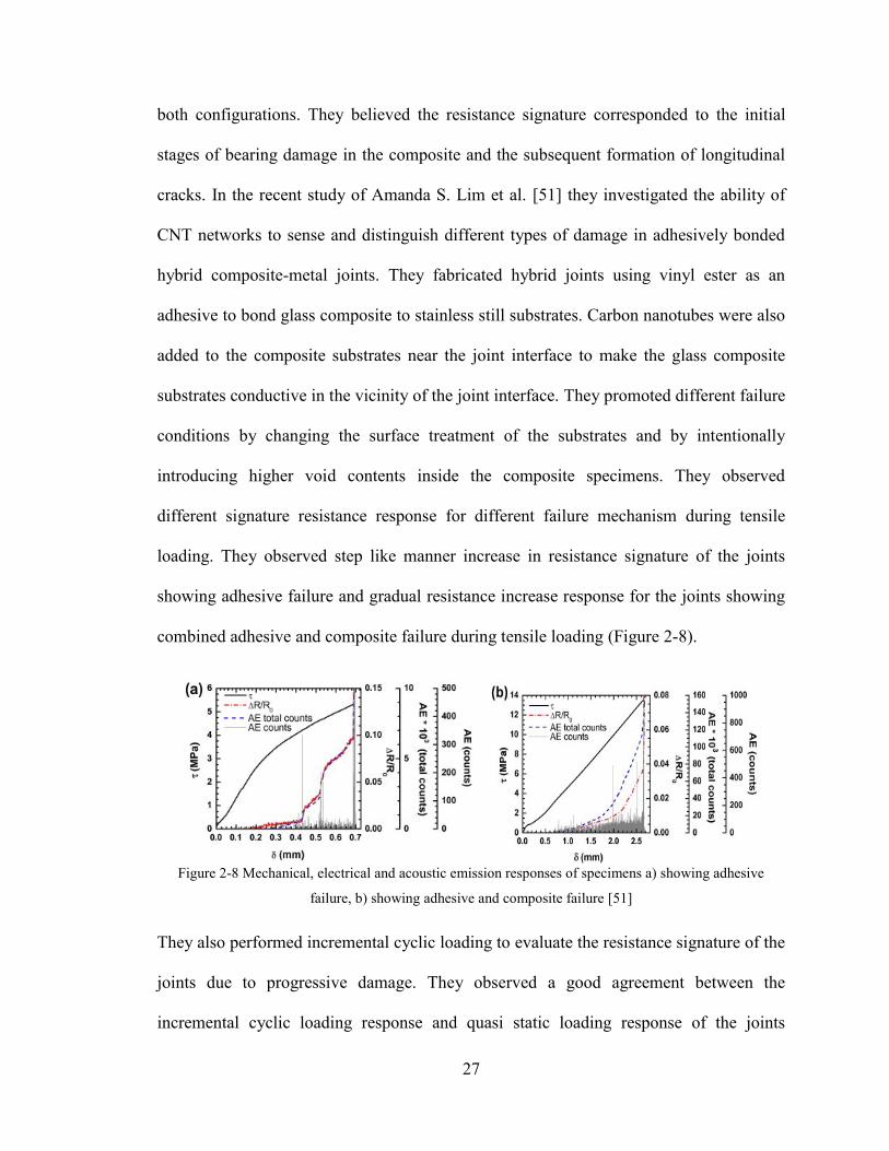
Figure 2-8 Mechanical, electrical and acoustic emission responses of specimens a) showing adhesive
failure, b) showing adhesive and composite failure [51] ............................................................................... 27
Figure 2-9 Mechanical and electrical response of specimens undergoing incremental cyclic loading
showing a) adhesive failure, b) adhesive and composite failure [51] ............................................................ 28
Figure 3-1 EPON 862 a) chemical b) molecular structures [54] ................................................................... 33
Figure 3-2 Epikure W chemical and molecular structures [54] ..................................................................... 34
Figure 3-3 Schematic of aluminum end tab ................................................................................................... 36
Figure 3-4 Schematic of aluminum substrate ................................................................................................ 36
Figure 3-5 Calendaring machine ................................................................................................................... 39
Figure 3-6 Vacuum oven ............................................................................................................................... 39
Figure 3-7 Alignment fixture ........................................................................................................................ 40
Figure 3-8 Single lap joint geometry ............................................................................................................. 40
Figure 3-9 Assembled single lap joint on the fixture .................................................................................... 41
Figure 3-10 Fixture to hold assembled single lap joints inside the oven for curing ...................................... 41
Figure 3-11 Assembled samples mounted on the fixture and ready to be cured ........................................... 41
Figure 3-12 Set up schematic of 4-probe technique ...................................................................................... 43
Figure 3-13 Set up schematic of 2-probe technique ...................................................................................... 43
Figure 3-14 Single lap joint aligned and mounted on the MTS machine using L shape guides .................... 44
xi
Figure 3-15 Fatigue test set-up ...................................................................................................................... 47
Figure 4-1 Joints electrical resistance for samples containing 0.5 wt% MWCNT ........................................ 50
Figure 4-2 Joints electrical resistance for samples containing 1 wt% MWCNT ........................................... 51
Figure 4-3 Resistance comparison between 0.5 and 1 wt% CNT loaded specimens .................................... 52
Figure 4-4 Joints electrical resistance for samples containing 2 wt% MWCNT ........................................... 52
Figure 4-5 Average electrical resistance comparison between the joints containing 0, 0.5, 1, and 2 wt%
MWCNT ....................................................................................................................................................... 54
Figure 4-6 Joint apparent shear strength for specimens containing no MWCNT ......................................... 55
Figure 4-7 Joint apparent shear strength for specimens containing 0.5 wt% MWCNT ................................ 56
Figure 4-8 Shear strength vs. electrical resistance for single lap joints containing 0.5 wt% MWCNT ......... 57
Figure 4-9 Joint apparent shear strength for specimens containing 1 wt% MWCNT ................................... 57
Figure 4-10 Shear strength vs. electrical resistance for single lap joints containing 1 wt% MWCNT .......... 58
Figure 4-11 Joint apparent shear strength for specimens containing 2 wt% MWCNT ................................. 58
Figure 4-12 Shear strength vs. electrical resistance for single lap joints containing 2 wt% MWCNT .......... 59
Figure 4-13 Average shear strength comparison between the joints containing 0, 0.5, 1, and 2 wt%
MWCNT ....................................................................................................................................................... 59
Figure 4-14 Fracture surface of specimens a) containing 0.5 wt% and b) 1 wt% MWCNT ......................... 61
Figure 4-15 Single lap joint fatigue life for specimens containing 0 wt% MWCNT .................................... 63
Figure 4-16 Single lap joints fatigue life distributions for specimens with 0 wt% MWCNT........................ 63
Figure 4-17 SEM image of a fracture surface of a sample containing no MWCNTs after the sample was
broken due to fatigue loading ........................................................................................................................ 64
Figure 4-18 Single lap joint fatigue life for specimens containing 0.5 wt% MWCNT ................................. 65
Figure 4-19 Single lap joints fatigue life distributions for specimens with 0.5 wt% MWCNT..................... 65
Figure 4-20 Single lap joint fatigue life for specimens containing 1 wt% MWCNT .................................... 66
Figure 4-21 Single lap joints fatigue life distributions for specimens with 1 wt% MWCNT........................ 67
Figure 4-22 Single lap joint fatigue life for specimens containing 1 wt% MWCNT .................................... 68
Figure 4-23 Single lap joints fatigue life distributions for specimens with different MWCNT loadings ...... 69
Figure 4-24 Single lap joints average fatigue failure cycles for different CNT loadings .............................. 69
xii
Figure 4-25 SEM images of fracture surface of a samples containing 0.5 wt% MWCNT showing CNT
bridging in different magnifications a) shows the fracture surface and b, c, and d show magnified images 70
Figure 4-26 SEM images of fracture surface of a samples containing 1 wt% MWCNT showing CNT
bridging in different magnifications a) shows the fracture surface and b, c, d and e show magnified images
....................................................................................................................................................................... 71
Figure 4-27 Electrical resistance signature vs. fatigue life of sample number 11 containing 0.5 wt%
MWCNTs (sample 0.5-11) ............................................................................................................................ 72
Figure 4-28 Electrical resistance ratio vs. fatigue life for sample 0.5-11 ...................................................... 73
Figure 4-29 Electrical resistance signature vs. fatigue life of sample number 15 containing 0.5 wt%
MWCNTs (sample 0.5-15) ............................................................................................................................ 73
Figure 4-30 Electrical resistance ratio vs. fatigue life for sample 0.5-15 ...................................................... 74
Figure 4-31 Electrical resistance signature vs. fatigue life of sample number 16 containing 0.5 wt%
MWCNTs (sample 0.5-16) ............................................................................................................................ 74
Figure 4-32 Electrical resistance ratio vs. fatigue life for sample 0.5-16 ...................................................... 75
Figure 4-33 Electrical resistance signature vs. fatigue life of sample number 21 containing 0.5 wt%
MWCNTs (sample 0.5-21) ............................................................................................................................ 75
Figure 4-34 Electrical resistance ratio vs. fatigue life for sample 0.5-21 ...................................................... 76
Figure 4-35 Electrical resistance signature vs. fatigue life of sample number 26 containing 0.5 wt%
MWCNTs (sample 0.5-26) ............................................................................................................................ 76
Figure 4-36 Electrical resistance ratio vs. fatigue life for sample 0.5-26 ...................................................... 77
Figure 4-37 Superposition of normalized electrical resistance ratios of the 5 example specimens containing
0.5 wt% MWCNT ......................................................................................................................................... 77
Figure 4-38 Average electrical resistance signatures of all 30 specimens containing 0.5 wt% MWCNTs ... 78
Figure 4-39 Slope of the average resistance signature curve from 60% of the life to 90% of the life .......... 79
Figure 4-40 SEM images of the fracture surface of a single lap joint containing 0.5 wt% MWCNTs and
evidence of multiple cracks (The image was taken after the sample was broken) ........................................ 81
xiii
Figure 4-41 Long-distance microscopic view of the edge of sample 0.5- 7, a) beginning of the test b)
bellow 60% of the fatigue life, c) first sign of delamination around 90% of the life, c) final failure at 30811
cycles ............................................................................................................................................................. 82
Figure 4-42 Long-distance microscopic view of the edge of sample 0.5- 10, a) beginning of the test b)
bellow 60% of the fatigue life, c) first sign of delamination around 85% of the life, c) final failure at 14350
cycles ............................................................................................................................................................. 83
Figure 4-43 Electrical resistance signature vs. fatigue life of sample number 4 containing 1 wt% MWCNTs
(sample 1-4)................................................................................................................................................... 84
Figure 4-44 Electrical resistance ratio vs. fatigue life for sample 1-4 ........................................................... 84
Figure 4-45 Electrical resistance signature vs. fatigue life of sample number 9 containing 1 wt% MWCNTs
(sample 1-9)................................................................................................................................................... 85
Figure 4-46 Electrical resistance ratio vs. fatigue life for sample 1-9 ........................................................... 85
Figure 4-47 Electrical resistance signature vs. fatigue life of sample number 10 containing 1 wt%
MWCNTs (sample 1-10) ............................................................................................................................... 86
Figure 4-48 Electrical resistance ratio vs. fatigue life for sample 1-10 ......................................................... 86
Figure 4-49 Electrical resistance signature vs. fatigue life of sample number 18 containing 1 wt%
MWCNTs (sample 1-18) ............................................................................................................................... 87
Figure 4-50 Electrical resistance ratio vs. fatigue life for sample 1-18 ......................................................... 87
Figure 4-51 Electrical resistance signature vs. fatigue life of sample number 19 containing 1 wt%
MWCNTs (sample 1-19) ............................................................................................................................... 88
Figure 4-52 Electrical resistance ratio vs. fatigue life for sample 1-19 ......................................................... 88
Figure 4-53 Superposition of normalized electrical resistance ratios of the 5 example specimens containing
1 wt% MWCNT ............................................................................................................................................ 89
Figure 4-54 The average electrical resistance signatures of all 30 specimens containing 1 wt% MWCNTs 89
Figure 4-55 Slope of the average resistance signature curve from 60% of the life to 90% of the life .......... 90
Figure 4-56 SEM images of the fracture surface of a single lap joint containing 1 wt% MWCNTs and
evidence of multiple cracks (The image was taken after the sample was broken) ........................................ 91
xiv
Figure 4-57 Long-distance microscopic view of the edge of sample 1- 6, a) beginning of the test b) bellow
60% of the fatigue life, c) first sign of delamination around 83% of the life, d) final failure at 10580 cycles
....................................................................................................................................................................... 93
Figure 4-58 Long-distance microscopic view of the edge of sample 1- 21, a) beginning of the test b) bellow
60% of the fatigue life, c) first sign of delamination around 88% of the life, d) final failure at 7041cycles . 93
Figure 4-59 Electrical resistance signature vs. fatigue life of sample number 1 containing 2 wt% MWCNTs
(sample 2-1)................................................................................................................................................... 95
Figure 4-60 Electrical resistance ratio vs. fatigue life for sample 2-1 ........................................................... 95
Figure 4-61 Electrical resistance signature vs. fatigue life of sample number 2 containing 2 wt% MWCNTs
(sample 2-2)................................................................................................................................................... 96
Figure 4-62 Electrical resistance ratio vs. fatigue life for sample 2-2 ........................................................... 96
Figure 4-63 Electrical resistance signature vs. fatigue life of sample number 3 containing 2 wt% MWCNTs
(sample 2-3)................................................................................................................................................... 97
Figure 4-64 Electrical resistance ratio vs. fatigue life for sample 2-3 ........................................................... 97
Figure 4-65 Electrical resistance signature vs. fatigue life of sample number 4 containing 2 wt% MWCNTs
(sample 2-4)................................................................................................................................................... 98
Figure 4-66 Electrical resistance ratio vs. fatigue life for sample 2-4 ........................................................... 98
Figure 4-67 Electrical resistance signature vs. fatigue life of sample number 5 containing 2 wt% MWCNTs
(sample 2-5)................................................................................................................................................... 99
Figure 4-68 Electrical resistance ratio vs. fatigue life for sample 2-5 ........................................................... 99
Figure 4-69 Superposition of normalized electrical resistance ratios of all 5 specimens containing 2 wt%
MWCNT ..................................................................................................................................................... 100
Figure 4-70 The average electrical resistance signatures of all 5 specimens containing 2 wt% MWCNTs 100
Figure 4-71 Slope of the average resistance signature curve from 60% of the life to 90% of the life ........ 101
Figure 4-72 Comparison between the electrical resistance signatures of samples containing 0.5, 1 and 2
wt% MWCNTs ............................................................................................................................................ 103
Figure 4-73 Fracture surface of a sample containing 0wt% MWCNTs which was broken after 19898 cycles.
(Sample 0-19) .............................................................................................................................................. 104
xv
Figure 4-74 Magnified image of the square area marked on Figure 4-73, a) 500μm, b) 100 μm ................ 105
Figure 4-75 Fracture surface of a sample containing 0wt% MWCNTs which was broken after 18193 cycles.
(Sample 0-17) .............................................................................................................................................. 106
Figure 4-76 Fracture surface of a sample containing 0wt% MWCNTs which was broken after 12726 cycles.
(Sample 0-11) .............................................................................................................................................. 107
Figure 4-77 Magnified image of the marked area on Figure 4-73 (b) ......................................................... 108
Figure 4-78 Fracture surface of a sample containing 0.5 wt% MWCNTs which was broken after 9200
cycles. (Sample 0.5-9) ................................................................................................................................. 109
Figure 4-79 Magnified image of marked section a) and b) on Figure 4-78 ................................................. 109
Figure 4-80 Fracture surface of a sample containing 0.5 wt% MWCNTs which was broken after 18193
cycles. (Sample 0.5-4) ................................................................................................................................. 110
Figure 4-81 Magnified image of the marked area (a) on Figure 4-80 ......................................................... 111
Figure 4-82 a) Fracture surface of a sample containing 0.5 wt% MWCNTs which was broken after 36000
cycles. (Sample 0.5-14) and b) magnified image of the square marked area (b) ......................................... 112
Figure 4-83 Fracture surface of a sample containing 1 wt% MWCNTs which was broken after 5255 cycles.
(Sample 1-29) .............................................................................................................................................. 113
Figure 4-84 Magnified image from the marked area a) and b) on Figure 4-83 ........................................... 113
Figure 4-85 a) Fracture surface of a sample containing 1 wt% MWCNTs which was broken after 14000
cycles. (Sample 1-28) and b) magnified image of the marked area on a).................................................... 114
Figure 4-86 Fracture surface of a sample containing 1 wt% MWCNTs which was broken after 135750
cycles. (Sample 1-13) .................................................................................................................................. 115
Figure 4-87 SEM image of glass bead on the fracture surface of a joint with 0 wt% MWCNTs ................ 116
Figure 4-88 SEM image of glass bead on the fracture surface of a joint with 0.5 wt% MWCNTs............. 116
Figure 4-89 SEM image of glass bead on the fracture surface of a joint with 1 wt% MWCNTs ................ 117

xvi
List of Tables
TABLE 2-1 Comparison between Non-Destructive and Destructive test methods [11] ............................... 11
TABLE 3-1 Components of 2024 T3 aluminum alloy [55] .......................................................................... 32
TABLE 3-2 Physical and mechanical properties of 2024 T3 aluminum alloy [55] ...................................... 32
TABLE 3-3 Physical and mechanical properties of EPON 862 [56] ............................................................ 33
TABLE 3-4 Physical properties of DETDA [56] .......................................................................................... 34
TABLE 3-5 MWCNT elements [58] ............................................................................................................. 34
TABLE 3-6 MWCNT typical properties [58] ............................................................................................... 35
TABLE 3-7 Surface pre-treatment detail [5] ................................................................................................. 37

1
Chapter 1
Introduction

2
1 Introduction
Adhesive joints are great alternatives to traditional mechanical joints due to their low
cost, low weight, and ease of manufacturing. They also minimize stress concentration by
uniformly distributing the stress though the contact surfaces. However, adhesively
bonded joints are more vulnerable to fatigue, and creep cracks and dynamic crack
propagation under cyclic loading are the primary reason for catastrophic failure in them
[1]. Although theoretically structures are designed with safe-life principles to withstand
catastrophic failures, damage detection is an important issue in maintenance of structures
especially of aircraft and space structures. Damages that are visible can easily be dealt
with and actions can be taken to maintain the integrity of the structures. On the other
hand, there are undetected and hidden damages which can be caused by low velocity
impacts and fatigues. The growths of these damages, which cause catastrophic failures,
are of great concern to end-users. Therefore, the design challenge for adhesive joints is
not only to increase their strength but to bring confidence in their safety; this confidence
can be obtained by in situ health monitoring and damage detection of the joint itself.
Little has been done to monitor the state of the adhesively bonded joints during its fatigue
life. Most researchers have focused on the effect of different parameters such as joint
thickness, overlap length, substrate thickness, existence of fillet in adhesive, and substrate
pre-treatment techniques on the fatigue life of the adhesive joints [2-6]. Since traditional
structural health monitoring (SHM) techniques require intensive human involvement and
are expensive, they are only applied in laboratory experiments rather than full size
structures. Moreover, structural polymeric adhesives are insulating material; therefore,
most of the traditional SHM techniques cannot be applied on them. However, carbon

3
nanotube-reinforced adhesives have superior electrical and mechanical properties than
neat adhesives; and there is growing interest in using carbon nanotubes (CNT) as in situ
sensors in composite structures to monitor the health of the structure itself. Introducing
carbon nanotubes inside polymeric adhesives create conductive networks which are
sensitive to damage and cracks inside the adhesive. Therefore, it is possible to monitor
the electrical resistance change of CNT-reinforced adhesively bonded joints and use the
electrical resistance signature as a mean to evaluate the state of the joints during their
service lives.
1.1 Motivations and Objectives
Due to their excellent specific properties aluminum has been widely used in aerospace
and automobile industries [7]. However, one of the challenges is to bond aluminum parts
to each other and to other materials. Since traditional bolted joints add to the weight of
the structures and create stress concentration in the joint area, adhesive bonds have been
introduced as alternatives to overcome these problems. Adhesive joints are, however,
susceptible to fatigue and creep cracks thus experiencing catastrophic failures [8]. Hence,
there is a need to increase their strength and provide an on-line monitoring technique to
bring in enough confidence for their use in high-tech industries.
In this study electrical resistance measurement technique is employed for in situ health
monitoring of adhesively bonded aluminum joints during fatigue loading using carbon
nanotube as in situ sensors. Aluminum is chosen as substrates materials since it is a
highly conductive metal. Therefore, the effectiveness of carbon nanotube network,
formed inside the adhesive, is evaluated for damage detection and the capability of the
technique to predict the residual life of the joints during fatigue testing is investigated.

4
Besides the electrical resistance monitoring technique, the electromechanical properties
of CNT-reinforced adhesively bonded joints using different CNT concentrations are
investigated and the results are compared to neat adhesive bonded joints to ensure that the
addition of carbon nanotubes inside the adhesive improves the electromechanical
properties of the joints.
Chapter two provides detailed literature about the structural health monitoring in general
and methods that have been developed to monitor adhesively bonded joints. It introduces
the electrical resistance method and the use of carbon nanotubes as in situ sensors to
detect damages in composite structures. The synthesis, properties and applications of
CNTs are also given in this chapter. The previous studies that have been carried out in the
area of damage detection and health monitoring of adhesive joints and composite
structures are explained briefly. The motivations and objectives of this thesis project are
given at the end of this chapter.
Chapter three explains the fabrication producers to produce single lap joints containing
different CNT concentrations. The test set up and procedures are also described in this
chapter.
The results for shear and fatigue tests and the in situ monitoring technique are presented
and discussed in detail in chapter four.
Chapter five presents the significant outcome of this thesis project and recommendation
for future works.

5
Chapter 2
Literature Review

6
2 Literature Review
2.1 Structural Health Monitoring
“Structural Health Monitoring (SHM) aims to give, at every moment during the life of a
structure, a diagnosis of the “state” of the constituent materials, of the different parts, and
of the full assembly of these parts constituting the structures a whole [9].” The diagnosed
status of the structure must remain in the design specification sphere, although the state
can change due to aging, to environmental conditions, and to incidents. Since the state is
monitored at every moment, the full history of the structure is recorded and with the help
of Usage Monitoring, prognosis (damage evolution, residual life, etc.) can also be
provided. By considering only the first function of SHM, diagnosis, one can say that
SHM is an improved way of Non-Destructive Evaluation (NDE). Although this
prospective towards SHM is partially true, SHM is much more. SHM can be considered
as a way to make artefact materials and structures smart. The concept of intelligent and
Smart Materials/Structures (SMS) found its application in civil and aeronautic industries
since the end of 1980s. In present day, they act as driving forces for innovation in all
industries. The SMS concept is a step in the general evolution of man-made objects from
simple to complex (Figure 2-1). Generally three types of SMS exist: SMS controlling
their shape, SMS controlling their vibration, SMS controlling their health. SHM
integrated structures and materials belong, at least in the short terms, to the less smart
type of SMS. Actually, the main achievements in SHM field are to make
materials/structures sensitive by embedding sensors. A simple but superficial analogy to
SHM structures is the nervous system of living beings. The embedded sensors in the

7
structures and the central processor are the nerves and the brain in living body,
respectively. The damage is detected by sensors then the central processor builds a
diagnosis and a prognosis and decides of the actions to undertake [9].
Figure 2-1General evolution of man-made objects from simple to complex [9]
2.1.1 Motivation
Continuous monitoring of technical structures is provided by the structural health
monitoring methodology. The early detection of damage by using SHM techniques leads
to prolonging the life of the aging structures. Moreover, understanding the real time
integrity of in-service structures is a very eminent purpose for manufacturer, end users,
and maintenance. The main benefits of SHM are as followings [9]:
Optimize use of the structure, minimize downtime, and prevention of catastrophic
failures,
Product improvement,

8
Drastic change in maintenance services: i) by replacing the scheduled and
periodic maintenance inspections with performance-based maintenance, and by
reducing the labour work; ii) by drastic reduction of human involvement,
therefore dropping labour, downtime and human errors.
The economical benefits of SHM systems are of prominent interests for end-users. In
effect, structures with SHM systems profit the end-users by constant maintenance cost
and constant reliability, whereas for classical structures without SHM maintenance cost
increases and reliability decreases (Figure 2-2).Moreover in aeronautic domain, due to
the permanent presence of sensors in structures, it is possible to reduce the safety margins
in some essential parts thus reducing the structure weight, improving the performance,
and lowering the fuel consumption [9].
Figure 2-2 Benefit of SHM for end users [9]

9
2.1.2 Passive and Active SHM
The SHM structures, embedded with sensors, interact with their surrounding environment
and their states and physical parameters are evolving. “Passive monitoring” is the case
that the examiner is just monitoring the evolution caused in the material without actuating
any perturbation in the structure. In “active monitoring” the examiner uses actuators to
perturb the structures parameters and then monitors the response of the structure [9].
2.1.3 NDE and SHM
The basis of SHM and NDE are the same. NDE techniques monitor the state of the
structures in specified intervals, whereas in SHM the state of the material is being
inspected throughout the life cycle of the structure at every moment. Therefore, by
integrating sensors and actuators inside the inspected structure and monitoring the
structure at every point in its service time, most NDE techniques can be transformed into
SHM techniques [9].
2.1.4 Non-Destructive Evaluation
Industrial products may consist of thousand components and parts. Every part within a
product has been designed to perform a function. The integrity of the whole product
depends upon the functionality of its individual parts. The ability of the part to perform
its function within an acceptable time period, which is one of the important user’s
expectations, is called its reliability. The part reliability depends upon multiple factors
such as design, raw materials, and manufacturing. These factors control the level of
defects in final products. There are also different flaws that may occur during the life
time of a component subjected to external loadings. The defects should be detected,
evaluated and monitored in manufacturing stages and throughout the product life service
10
to increase its level of quality. High product quality increases the reliability of the
product and in turn the safety of the machines, thus bringing economic returns to the
clients. Therefore, there is need to have techniques to examine and control the defects in
the products without impairing their functionality. These techniques can be categorized
into two general classes: destructive and non-destructive. Destructive methods are based
on fracture mechanics and the specimen tested will be destroyed [10,11]. It is interesting
to compare the non-destructive test method with destructive ones to better understand the
important aspects of NDT (TABLE 2-1) [10,11].
NDT methods range from simple to complex. The simplest one is visual inspection. If
multiple surface defects are detected by this method, there is often little need to use more
complicated methods. More than one technique is usually used to detect the whole
structure or sometimes one technique should be used to confirm and validate the results
obtained from another one [10,11].
Although "non-destructive testing has no clearly defined boundaries", R. Halmshaw,
1991, the most commonly NDT methods used in industry are as followings: visual
inspection, liquid penetrant inspection, magnetic particle inspection, eddy current testing,
ultrasonic testing, radiology, acoustic emission, alternating current potential drop,
alternating current field measurement, and thermography [10,11]. “Each NDT method is
especially suited for a particular task and hence does not compete with, but complement
each other [11]”.

11
Non-Destructive Destructive
Limitations
Need to verify the reliability of
the measurements
Qualitative measurement
Experienced and expert inspector
required to interpret the results
Advantages
Test can be done directly on the
components
Many NDT can be done on one
part and all properties can be
measured
In situ testing
Test can be repeated
Little preparation
Rapid
Advantages
Reliable measurements
Quantitative
Direct correlation between test
measurements and material
properties
Limitation
Tests are not done on the
components directly
One or few properties can be
measured by one test
In service measurement is not
possible
In service property change cannot
be measured
Time consuming and costly
TABLE 2-1 Comparison between Non-Destructive and Destructive test methods [11]
2.2 Structural Health Monitoring in Adhesively Bonded Joints
In complex structures, due to size limitations and manufacturing processes, presence of
joints is inevitable [7,12]. Conventional bolted joints create stress concentration thus
reduce the integrity of the structures. Besides the integrity reduction, bolted joints add to
the weight of the structures therefore increase the fuel consumption [12].Adhesively
bonded joints, as substitutes to traditional mechanical joints, have been extensively used

12
in aerospace, electrical, and automotive industries due to the low cost, low weight, and
ease of manufacturing [7]. Contrary to traditional joints, in adhesive joint the stress is
distributed through the contact surfaces between the two jointed pieces thus minimizing
stress concentration [7-12]. Moreover, adhesive bonding enables the possibility of joining
dissimilar materials. However, adhesive joints have some drawbacks such as, substrate
surface pretreatment requirement to improve the adhesion and the inability of the joint to
be disassembled for maintenance and damage inspection [7-12].Adhesive joints are also
more susceptible to creep and fatigue cracks and catastrophic failure is common between
them [7-13]. Therefore, it is highly required to monitor the state of the joint throughout
its service life. This section provides detail literature about the techniques that were used
to monitor adhesively bonded joints and also techniques which were used to monitor
bolted joints that could be employed for adhesive joints as well. Jacek M. et al. [14]
investigated an ultrasonic method to monitor bonding processes and evaluation of the
cold setting adhesive bonded wood laminates. They concluded that the acoustic
transmission was sensitive to different bond types and curing phases and it was
reasonably correlated with bond strength development. Shuo Yang et al. [15] applied a
vibration damping and frequency measurements as a non-destructive method to detect
weak joints in adhesively bonded composite sandwich beams. They proposed that the
vibration frequencies and mode shapes depend upon joint stiffness and mass; and since
structure mass and stiffness change due to damage and defects, the difference in vibration
frequencies and mode shapes between the defect free structure and damaged structure can
be utilized as a mean to detect degraded bonds. They concluded that the technique is an
effective method in detecting damage in bonded joints however; damping measurement
13
appears to be more reliable. T. Mickens et al. [16] investigated a single-based vibration
method to detect, locate and approximately quantify damage in an aircraft wing tip. They
bonded four piezoelectric patches on the wing root to send and receive vibration signals
alternatively. They stimulated the damage by loosening of the screw joints or rivets. They
observed the change in stiffness due to promoted damage affected the local vibration
response in high frequencies. R. Jones et al.[17] investigated the application of fiber Brag
grating (FBG) sensors in monitoring the structural health of a composite repair attached
to aluminum skins separated by a honeycomb sandwich core. The fiber optic sensors
were attached to the composite repair and aluminum skin and the change in their
wavelength, which is the key mean to measure strain, were measured precisely. They
observed that the strain increased as the crack propagates towards the optic sensors and
continued to increase as it passed them. Their study demonstrated the capability of optical
sensor arrays to monitor crack growth. C.J. Brotherhood et al. [18] examined three
different ultrasonic methods namely as, conventional normal incident longitudinal and
shear wave and a high power ultrasonic method to detect kissing bonds in adhesive joints.
Kissing bond is a term referred to a failure mechanism in adhesive bonds caused due to
poor adhesion between adhesive layer and the substrates. Their study demonstrated that
the high power ultrasonic technique was more sensitive at low contact pressures to detect
kissing bonds, while conventional longitudinal wave inspection were more effective for
higher contact pressures. However, they suggested that combination of two or more
ultrasonic techniques could improve the quality assessment of the bonded joints. I.
Hersberg et al. [19, 20] assessed optical fiber Bragg grating sensors for structural health
monitoring of glass fiber reinforced polymer composite T-joints. They developed a
14
technique to embed and position optical fibers successfully into the joint interface. “The
Bragg grating is designed to reflect only a narrow band of wavelengths propagating in the
fiber;” Therefore, as the fiber is strained, the reflected wavelength changes. They also
performed a finite element modeling to determine the strain distribution due to artificially
disbond the T-joint and compared the analytical data with the experimental results. They
concluded that the fiber Brag grating sensors along with FEM analysis could be
promising means for damage assessment. J. Palaniappan et al. [21, 22] embedded chirped
fiber Bragg grating within an adherend in adhesively bonded composite joints to monitor
the integrity of the structure. They proposed that the changes in reflected spectra of the
embedded sensors could be used to monitor disbonding in composite joints. In this study
the composite joint was subjected to cyclic loading and monitored using embedded
sensors. They observed a shift of the low-wavelength end of the reflected spectrum to
lower wavelengths as disbond initiated, whereas, the disbond growth caused a movement
of perturbation towards higher wavelengths. Baruch Karp et al. [23] studied the end
effect of a cantilever beam by attaching surface strain gages at the immediate vicinity of
the joint. They observed that the end effects measured through surface strain gages could
identify small changes in the clamping condition. Ze Zhang et al.[24] investigated the
capability of stiffness degradation measurement on fatigue life prediction of adhesively
bonded composite joints. They concluded that linear stiffness degradation occurred due to
fatigue loading. They observed a critical stiffness and elongation at which failure
occurred. Renos et al. [25] assessed a vibration based technique using impulse hammer
response method for damage detection in bonded composite pultruded sections. They
observed that the technique was only sensitive to significant damage. Timothy et al. [26,
15
27] proposed chaotically amplitude-modulated ultrasonic waves method combined with
time series algorithms to locate damage and classify damage conditions in composite
skin-to-spar joints. Piezoelectric patches were attached to the composite joints and
ultrasonic waves were imparted to the structure and the structural response was recorded.
They concluded that the technique was capable of detecting small level of damage even
for complicated geometries. Ivan et al. [28] evaluated an analytical method to monitor the
bolted joints using electrical conductivity measurement. They concluded that their
theoretical study is useful for detecting loosening failure in bolted joints. Frank Balle et
al. [29] employed electrical resistance measurement technique for damage assessment of
ultrasonically welded aluminum/carbon-fiber joints. Since the fibers were directly welded
to the aluminum substrate it made it possible to monitor the change in electrical
resistance during fatigue. They realized that this technique was sensitive to micro-
structural damages and had better results compare to the results from strain gages
attached to the surface of the aluminum. Andrea et al. [30] studied the capability of
embedded fiber Brag grating sensors to monitor fatigue crack growth in composite
adhesively bonded joints. They embedded array of optic sensors to the side of the single
lap tapered joint in thick composite laminate. Their study demonstrated that the optical
sensors were capable of detecting and monitoring crack propagation during fatigue test
even in the case that crack propagated through the plies of the thick composite laminate.
The techniques that were used to monitor the state of the joints in described articles can
be categorized into 5 general methods as follow: 1) ultrasonic base, 2) vibration base, 3)
mechanical property measurement, 4) fiber optic (strain base), and5) electrical resistance
measurements.

16
In ultrasonic base techniques ultrasonic and acoustic waves are propagated through the
materials using an actuator most preferably piezoelectric ones and the response of the
material is recorded using the same actuator or a receiver sensor which is another
piezoelectric patch. The response of the material changes due to damage and cracks;
hence it can be used as a mean to assess the state of the structure. Ultrasonic techniques
are sensitive to small cracks and have good resolution. However, the technique has
several drawbacks; it requires sensors to be attached to the structures therefore, the
surface of the structure should be available and the technique is capable to locally
detecting the damage since sensors cannot be attached to the whole structure. It needs
sophisticated instrumentation and expert examiner which makes the technique highly
expensive. It posses high downtime since the technique usually cannot be used as on line
health monitoring technique [18,26, 27].
Vibration base methods, uses the vibration and damping response of the structures to
detect damage and defects inside the materials. The change in the microscopic structures
of the materials due to damage, aging, and environmental condition, alter the vibration
and damping responses of the structure. This technique is sensitive and has good
resolution however it is difficult to distinguish the aging and environmental effects on the
structural responses from that of damage effects; hence, the technique needs analytical
calculation to distinguish the differences. The technique needs expert examiner and
expensive instruments and is often used as offline health monitoring technique [15,
16,25].
Mechanical property measurement technique, measures the change in mechanical
properties of the structure throughout its service life. The change in mechanical

17
properties can be correlated with damages occurred inside the structure. The technique is
capable of predicting an allowable property reduction such as stiffness reductions which
is correlated to the state of the structure. However, the technique requires sophisticated
equipments, complicated set-up and extensive calculations [23-24].
Strain base techniques, uses strain sensors to record the strain changes in the structures
due to damage occurrence and crack initiation and propagations. There is a growing
interest in using fiber optic sensors as strain sensors to monitor structures especially civil
structures. They are attached on the surface of the structures or embedded inside them.
They only reflect specific wavelengths and as crack initiates and propagates the strain
caused in the optic sensors changes the wavelength and the change in wavelength can be
correlated to damage. The technique is sensitive to superficial cracks and damages and is
capable of detecting damages in the vicinity of the sensors. The technique, however, can
be used as a potentially promising in situ monitoring technique. The main challenge is to
embed the fiber optics, due to their micron size, inside the materials without degradation
of the structure; and for the attached sensors the main challenge is to protect them from
external loading and environmental conditions. The technique is expensive; nonetheless,
the growing interest in using them in high tech industries such as civil and aerospace may
lead to the technique to become inexpensive and justify their use in online health
monitoring of the structures [17,19,22, 30,31].
Electrical resistance monitoring technique, records the change in electrical resistance of
the structure due to inside damage. It does not require sophisticated instrumentation and
is inexpensive; it is used as on line health monitoring technique. The technique requires
the structure to be conductive. Nonetheless, the technique is greatly sensitive in
18
conductive composite materials since they are inherently sensitive materials. Therefore,
electrical resistance monitoring technique is an excellent monitoring technique to be used
as in situ techniques for conductive composite materials [9,29].
2.3 Electrical Resistance Monitoring Using Sensors
As discussed in previous section many of the classical NDE and SHM techniques, which
are used for periodic maintenance, require extensive human labor and expensive
procedures. Moreover, the accidents and failures which occur between successive
overhauls will not be detected in periodic inspection. Therefore, there is rising interest in
developing sensitive materials or structures with ability to provide real-time information
about the material itself. To obtain sensitive materials one natural way is to use the
material itself as a sensor. Clearly, Carbon Fiber (CF) and Carbon Nanotubes (CNT)
composites are amongst these sensitive materials. Since carbon fibers and carbon
nanotubes are conductive materials the measurement of the global electrical resistance of
the composite structures containing CF or CNT can be a promising technique for
monitoring the composite structural integrity. In carbon fiber composite laminates the
fiber breakage, fiber/matrix debonding, matrix microcracks, and delamination contribute
to electrical resistance increase. Therefore, monitoring the electrical resistance change
can give valuable information about the formation of defects and their severity. In
randomly distributed carbon fiber or carbon nanotubes composites the electrical threshold
plays an important role. Since polymer adhesives are insulating matrices (ρ ≈ 1013
to 1015
Ωm) the composite electrical conductivity varies dramatically from a critical
reinforcement rate or percolation threshold, which corresponds to the formation of
continuous conducting path by conducting particles thus making the composite

19
conductive. This conductive path can form by real contact between the particles or by the
inter-particle tunneling effect which in fact the current goes through a thin layer of
polymer. The formation of cracks inside conductive composites breaks the conductive
path thus increases electrical resistance. This technique needs neither sophisticated
equipment nor extensive human involvement. It has promising future in composite
materials and structures in on line health monitoring [9]. Moreover, it is important to
mention that carbon Nanotubes (CNT) attracts the attention of many researchers due to
its multifunctional properties [32-41]. CNT reinforced polymer adhesives have shown
superior electromechanical properties compared to neat adhesives. Therefore, electrical
resistance measurement technique can be utilized to monitor the structural health of
adhesively bonded joints reinforced with carbon nanotubes. The following section
provides detail about carbon nanotubes, its synthesis, and its incorporation inside
polymer adhesives.
2.3.1 Carbon Nanotubes
2.3.1.1 Introduction
Carbon nanotubes (CNTs) are fullerene structures, geometrical cage-like structures.
Fullerenes were first developed by Smalley and co-workers in mid 1980s [32]. This
discovery led to the synthesis of carbon nanotubes by Iijima in 1991 [33]. Carbon
nanotubes can be considered as rolled graphite sheets into cylinders. Graphite is a 2-D
sheet of carbon atoms. Each carbon atom is connected to three other carbon atoms in its
neighborhood. Thus the interconnected networks of carbon atoms arrange hexagonal
arrays. Rolling graphite sheets form different nanotube structures. These different
structures are distinguished by their chirality. Chiral vector can be envisaged as a vector
20
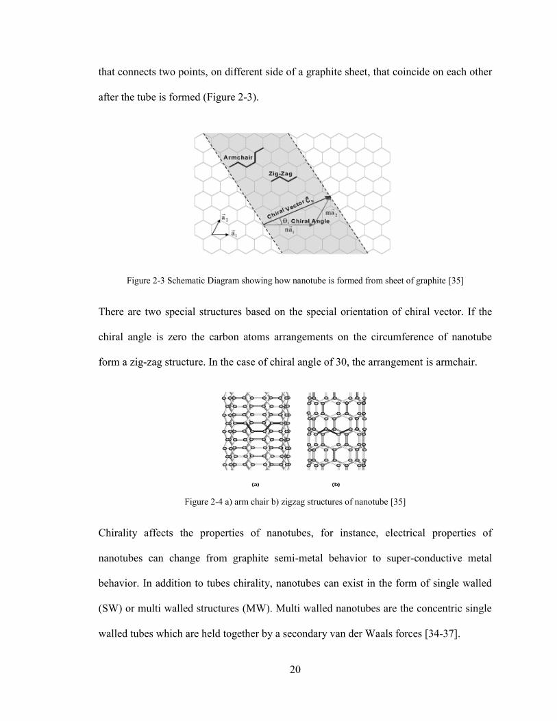
that connects two points, on different side of a graphite sheet, that coincide on each other
after the tube is formed (Figure 2-3).
Figure 2-3 Schematic Diagram showing how nanotube is formed from sheet of graphite [35]
There are two special structures based on the special orientation of chiral vector. If the
chiral angle is zero the carbon atoms arrangements on the circumference of nanotube
form a zig-zag structure. In the case of chiral angle of 30, the arrangement is armchair.
Figure 2-4 a) arm chair b) zigzag structures of nanotube [35]
Chirality affects the properties of nanotubes, for instance, electrical properties of
nanotubes can change from graphite semi-metal behavior to super-conductive metal
behavior. In addition to tubes chirality, nanotubes can exist in the form of single walled
(SW) or multi walled structures (MW). Multi walled nanotubes are the concentric single
walled tubes which are held together by a secondary van der Waals forces [34-37].
21
2.3.1.2 Carbon Nanotube Synthesis
There are different methods for synthesis of single wall and multi wall carbon nanotubes.
These methods include arc-discharge, laser ablation, gas catalytic growth from carbon
monoxide, and chemical vapor deposition (CVD) from hydrocarbons. Arc-discharge
technique, first used by Iijima to synthesis nanotubes, comprises of purely graphite rods
as cathode and anode which are brought together to produce a stable arc. Synthesized
carbon nanotube then deposits on cathode along with shell of fused material. Other
procedures are required to separate the carbon nanotubes from the impurities. Laser
ablation was first used to synthesize fullerenes. In this technique a laser beam is used to
vaporize the graphite target held in an elevated temperature of 1200°C and controlled
environment. The carbon nanotubes are then deposited on a collector. Since the source of
graphite, the anode in arc and the target in laser, is limited, the high cost of high scale
productions of CNTs is prohibitive. This major drawback led to developing better and
cheaper techniques for scaled up productions of CNTs. Gas-phase and chemical vapor
deposition solved this problem. In these techniques the source of the carbon is the carbon
carrying gas which can be fed continually to the system by flowing gas. CVD is the most
common method to synthesize nanotubes in which a hydrocarbon gas (methane, carbon
monoxide, and acetylene) is decomposed on a metal substrate (Ni, Fe, or Co) and
produces multiwall carbon nanotube. The advantages of the CVD technique are its high
purity of the byproduct CNTs and also its ability to produce aligned arrays of carbon
nanotubes [34, 37].
22
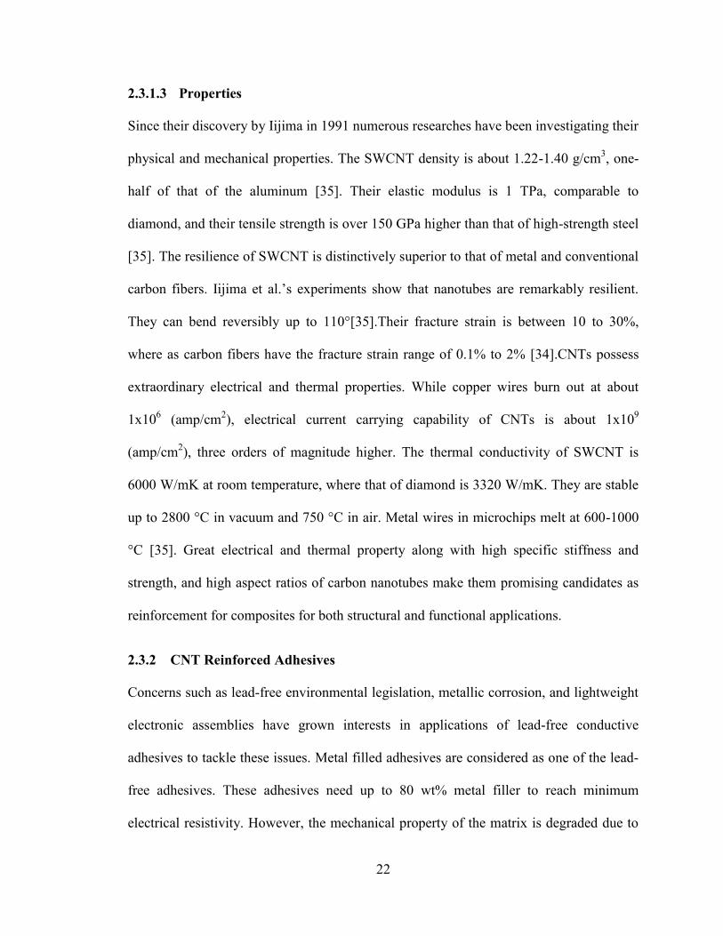
2.3.1.3 Properties
Since their discovery by Iijima in 1991 numerous researches have been investigating their
physical and mechanical properties. The SWCNT density is about 1.22-1.40 g/cm3, one-
half of that of the aluminum [35]. Their elastic modulus is 1 TPa, comparable to
diamond, and their tensile strength is over 150 GPa higher than that of high-strength steel
[35]. The resilience of SWCNT is distinctively superior to that of metal and conventional
carbon fibers. Iijima et al.’s experiments show that nanotubes are remarkably resilient.
They can bend reversibly up to 110°[35].Their fracture strain is between 10 to 30%,
where as carbon fibers have the fracture strain range of 0.1% to 2% [34].CNTs possess
extraordinary electrical and thermal properties. While copper wires burn out at about
1x10⁶ (amp/cm
2), electrical current carrying capability of CNTs is about 1x10
9
(amp/cm2), three orders of magnitude higher. The thermal conductivity of SWCNT is
6000 W/mK at room temperature, where that of diamond is 3320 W/mK. They are stable
up to 2800 °C in vacuum and 750 °C in air. Metal wires in microchips melt at 600-1000
°C [35]. Great electrical and thermal property along with high specific stiffness and
strength, and high aspect ratios of carbon nanotubes make them promising candidates as
reinforcement for composites for both structural and functional applications.
2.3.2 CNT Reinforced Adhesives
Concerns such as lead-free environmental legislation, metallic corrosion, and lightweight
electronic assemblies have grown interests in applications of lead-free conductive
adhesives to tackle these issues. Metal filled adhesives are considered as one of the lead-
free adhesives. These adhesives need up to 80 wt% metal filler to reach minimum
electrical resistivity. However, the mechanical property of the matrix is degraded due to
23
the high metal filler loading [38]. Therefore CNT-reinforced adhesives become
promising in replacing metal filled ones. The electro-mechanical properties of CNT-
reinforced adhesives were reported to be superior to neat adhesive by many researchers.
Sangwook et al. [39] studied the through thickness thermal conductivity in aligned
carbon nanotubes adhesive bond. They study revealed significant enhancement of
bonding performance as well as improvement in through thickness thermal conductivity.
They reported 32 and 45 % increase in shear strength by adding 1 and 5 w% of CNT,
respectively. In the study of Suzhu et al. [40] it was observed that the percolation
threshold as low as 0.5 w% CNTs was enough to make the insulating adhesive
conductive. The study of Suzhu et al. [42] showed that the addition of CNTs to the epoxy
significantly enhanced the durability of adhesive joint. It was revealed that at an optimum
value of approximately 1 wt% CNTs maximum increase in joint durability could be
achieved. However, L. Roy et al. [43] did not achieve great increase in adhesive
mechanical strength by incorporating CNTs. H.P. Wu et al. [44] compared 2 different
isotropical conductive adhesives (ICA) developed by MWCNT and silver coated CNT
(SCCNT) with traditional ICA. They reported better conductivity and shear strength for
both SCCNT and MWCNT compared to traditional ICA. Kuang et al. [45] investigated
the use of epoxy/MWCNT as adhesive to joint composite substrates and concluded that
there was 45.6% increase in the joint shear strength while adding 5 w% MWCNT.
2.4 Damage Detection and Prognosis Using CNT Networks or Sensors
Baughman et al. [46] first reported the intrinsic coupling between the electrical and
mechanical properties of CNT which makes them outstanding candidates for in situ
sensing. Chunyu Li et al. [47] studied the use of CNT as mechanical sensors in variety of

24
sensing applications such as mass, strain, humidity, and temperature sensors.
Thonstenson et al. [48] demonstrated in their study that carbon nanotubes forms
conductive network in an epoxy and this conductive network can be utilized as highly
sensitive sensors for detecting the onset, nature, and evaluation of damage in advanced
polymer-based composites. They performed tensile tests on nanotube/epoxy specimens
and monitored the specimen electrical resistance by highly sensitive voltage-current
meter. They observed a highly linear relationship between the specimen deformation and
electrical resistance, (Figure 2-5).
Figure 2-5 Resistance change with deformation for a 0.5 w% nanotube epoxy composite loaded in tension
[48]
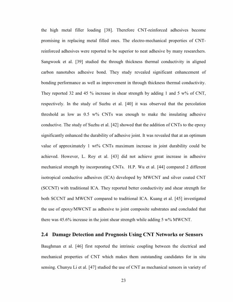
They produced 0 unidirectional and 0/90 cross ply laminates consisting of 5 plies with a
cut in the middle lamina to promote ply delamination during tensile testing. They
observed linear increase in both specimen configuration resistances due to initial
deformation followed by a sharp increase in resistance with initiation of delamination
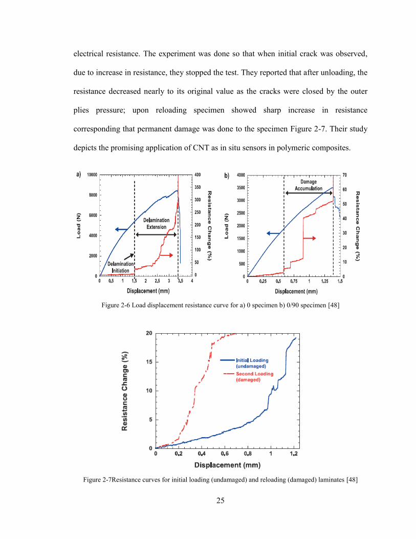
Figure 2-6. They also investigated the effect of loading, un-loading, and reloading on
25
electrical resistance. The experiment was done so that when initial crack was observed,
due to increase in resistance, they stopped the test. They reported that after unloading, the
resistance decreased nearly to its original value as the cracks were closed by the outer
plies pressure; upon reloading specimen showed sharp increase in resistance
corresponding that permanent damage was done to the specimen Figure 2-7. Their study
depicts the promising application of CNT as in situ sensors in polymeric composites.
Figure 2-6 Load displacement resistance curve for a) 0 specimen b) 0/90 specimen [48]
Figure 2-7Resistance curves for initial loading (undamaged) and reloading (damaged) laminates [48]
26
M. Nofar et al. [49] reported the sensing capability of CNT network in detecting the
failure region in laminated composite subjected to static and dynamic loading. They also
studied the difference of sensitivity between strain gauges and CNT network inside the
polymer. They concluded that the CNT network is more sensitive in detecting and
predicting the cracked regions than strain gauges due to existence of CNT network
throughout the structure as whole rather than locally attached strain gauges that are only
able to detect cracks in selected areas. Limin Gao et al. [50] studied the integration of
carbon nanotube inside glass fiber laminated composite to detect the formation of
microscale damage and evaluate the damage evolution and failure mechanisms in cyclic
loading. They also reported that electrical resistance measurement of carbon nanotube
network is a potential non invasive technique to sense damage in composite structures.
W. Zhang et al. [1] investigated the sensitivity potential of volume and through thickness
resistance measurement of CNT reinforced graphite fiber composites in monitoring
delamination. They observed that CNT network was highly sensitive to the delamination
length, showing that CNT additives could be used as real time sensors to size the
delamination and monitor its growth rate. The same technique can be used for in service
health monitoring of adhesively bonded metal-metal, metal-composite, and composite-
composite joints. Thostenson et al. [13] reported “the unique capability of carbon
nanotube network as in situ sensors for sensing local composite damage and bolt
loosening in mechanically fastened glass/epoxy composite joints.” They examined the
single lap and double lap configuration specimens and measured the electrical resistance
change due to applied loading. They observed linear increase in electrical resistance till
approximately 60% of the ultimate load followed by deviation from linear increase in
27
both configurations. They believed the resistance signature corresponded to the initial
stages of bearing damage in the composite and the subsequent formation of longitudinal
cracks. In the recent study of Amanda S. Lim et al. [51] they investigated the ability of
CNT networks to sense and distinguish different types of damage in adhesively bonded
hybrid composite-metal joints. They fabricated hybrid joints using vinyl ester as an
adhesive to bond glass composite to stainless still substrates. Carbon nanotubes were also
added to the composite substrates near the joint interface to make the glass composite
substrates conductive in the vicinity of the joint interface. They promoted different failure
conditions by changing the surface treatment of the substrates and by intentionally
introducing higher void contents inside the composite specimens. They observed
different signature resistance response for different failure mechanism during tensile
loading. They observed step like manner increase in resistance signature of the joints
showing adhesive failure and gradual resistance increase response for the joints showing
combined adhesive and composite failure during tensile loading (Figure 2-8).
Figure 2-8 Mechanical, electrical and acoustic emission responses of specimens a) showing adhesive
failure, b) showing adhesive and composite failure [51]
They also performed incremental cyclic loading to evaluate the resistance signature of the
joints due to progressive damage. They observed a good agreement between the
incremental cyclic loading response and quasi static loading response of the joints
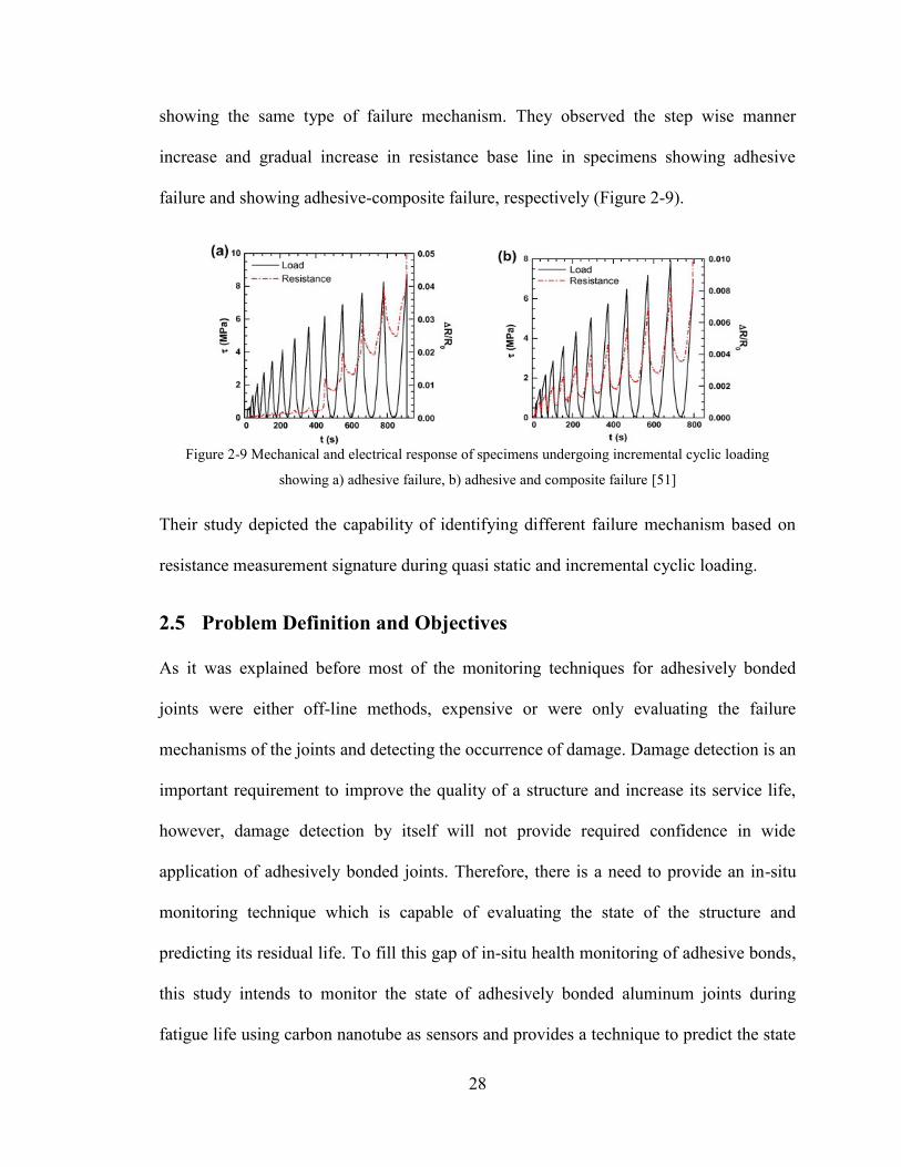
28
showing the same type of failure mechanism. They observed the step wise manner
increase and gradual increase in resistance base line in specimens showing adhesive
failure and showing adhesive-composite failure, respectively (Figure 2-9).
Figure 2-9 Mechanical and electrical response of specimens undergoing incremental cyclic loading
showing a) adhesive failure, b) adhesive and composite failure [51]
Their study depicted the capability of identifying different failure mechanism based on
resistance measurement signature during quasi static and incremental cyclic loading.
2.5 Problem Definition and Objectives
As it was explained before most of the monitoring techniques for adhesively bonded
joints were either off-line methods, expensive or were only evaluating the failure
mechanisms of the joints and detecting the occurrence of damage. Damage detection is an
important requirement to improve the quality of a structure and increase its service life,
however, damage detection by itself will not provide required confidence in wide
application of adhesively bonded joints. Therefore, there is a need to provide an in-situ
monitoring technique which is capable of evaluating the state of the structure and
predicting its residual life. To fill this gap of in-situ health monitoring of adhesive bonds,
this study intends to monitor the state of adhesively bonded aluminum joints during
fatigue life using carbon nanotube as sensors and provides a technique to predict the state

29
of the joints at each moment or in other words predict the residual life of the joints. In our
study, Epon 862 is used as an adhesive to join aluminum substrates. Carbon nanotubes as
sensors are added to the adhesive to make it conductive then the electrical resistance
signature of the joints containing different concentration of carbon nanotubes are
monitored during fatigue test. The results are evaluated to assess the effectiveness of
carbon nanotube network as in situ sensors to monitor the health of the adhesively
bonded joints and predict their residual life.

30
Chapter 3
Experimental
31
3 Experimental
3.1 Introduction
As it was mentioned in previous chapters, joints are essential parts in complex structures
thus they have to be designed to withstand service loadings and environment. Since
bolted joints add to the weight of the structures, adhesive joints can be used as promising
alternatives. However, adhesive joints cannot be disassembled for periodic maintenance,
therefore, it is essential to provide a structural health monitoring technique to evaluate the
state of the joints throughout their service life. Nevertheless most of the available
structural health monitoring techniques requires the materials to be electrically
conductive, while adhesives are naturally insolating materials. Hence, MWCNTs can be
introduced to adhesive joints to make them conductive. In this study we developed a
technique, using carbon nanotube network, to evaluate the health of single lap joints
during fatigue life. Despite of the fact that this study focuses on the structural health
monitoring of adhesively bonded joints, it is of prime importance to make sure that the
addition of MWCNTs does not degrade the mechanical properties of the joints.
Therefore, single lap joints were fabricated and mechanically tested to assess the
capability of our technique in monitoring the health of the structure and also to evaluate
the mechanical properties of the joints containing MWCNT. This chapter describes in
detail, the materials used and their properties, the sample fabrication, and the
experimental procedures.
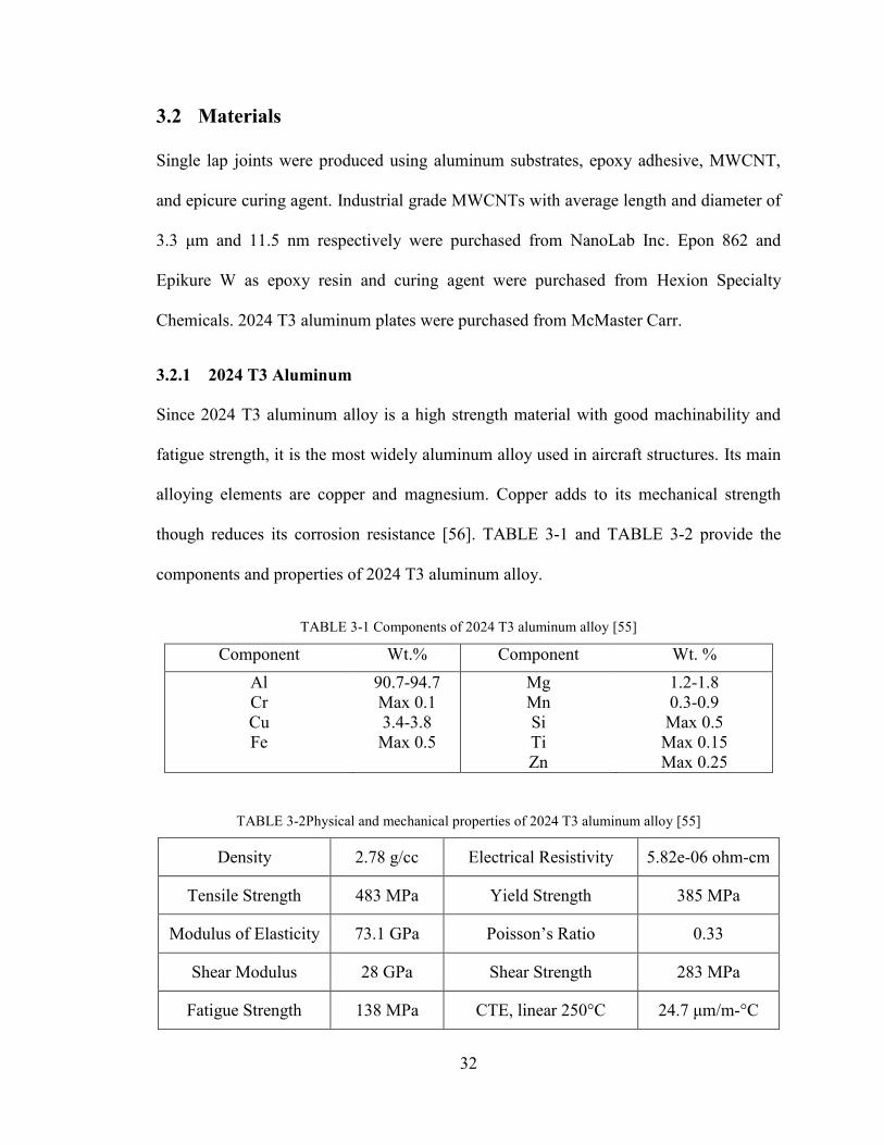
32
3.2 Materials
Single lap joints were produced using aluminum substrates, epoxy adhesive, MWCNT,
and epicure curing agent. Industrial grade MWCNTs with average length and diameter of
3.3 μm and 11.5 nm respectively were purchased from NanoLab Inc. Epon 862 and
Epikure W as epoxy resin and curing agent were purchased from Hexion Specialty
Chemicals. 2024 T3 aluminum plates were purchased from McMaster Carr.
3.2.1 2024 T3 Aluminum
Since 2024 T3 aluminum alloy is a high strength material with good machinability and
fatigue strength, it is the most widely aluminum alloy used in aircraft structures. Its main
alloying elements are copper and magnesium. Copper adds to its mechanical strength
though reduces its corrosion resistance [56]. TABLE 3-1 and TABLE 3-2 provide the
components and properties of 2024 T3 aluminum alloy.
TABLE 3-1 Components of 2024 T3 aluminum alloy [55]
Component Wt.% Component Wt. %
Al
Cr
Cu
Fe
90.7-94.7
Max 0.1
3.4-3.8
Max 0.5
Mg
Mn
Si
Ti
Zn
1.2-1.8
0.3-0.9
Max 0.5
Max 0.15
Max 0.25
TABLE 3-2Physical and mechanical properties of 2024 T3 aluminum alloy [55]
Density 2.78 g/cc Electrical Resistivity 5.82e-06 ohm-cm
Tensile Strength 483 MPa Yield Strength 385 MPa
Modulus of Elasticity 73.1 GPa Poisson’s Ratio 0.33
Shear Modulus 28 GPa Shear Strength 283 MPa
Fatigue Strength 138 MPa CTE, linear 250°C 24.7 μm/m-°C
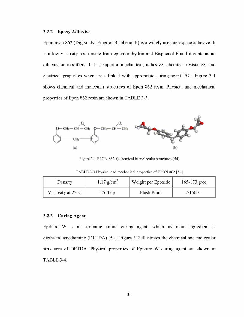
33
3.2.2 Epoxy Adhesive
Epon resin 862 (Diglycidyl Ether of Bisphenol F) is a widely used aerospace adhesive. It
is a low viscosity resin made from epichlorohydrin and Bisphenol-F and it contains no
diluents or modifiers. It has superior mechanical, adhesive, chemical resistance, and
electrical properties when cross-linked with appropriate curing agent [57]. Figure 3-1
shows chemical and molecular structures of Epon 862 resin. Physical and mechanical
properties of Epon 862 resin are shown in TABLE 3-3.
Figure 3-1 EPON 862 a) chemical b) molecular structures [54]
TABLE 3-3 Physical and mechanical properties of EPON 862 [56]
Density 1.17 g/cm3
Weight per Epoxide 165-173 g/eq
Viscosity at 25°C 25-45 p Flash Point >150°C
3.2.3 Curing Agent
Epikure W is an aromatic amine curing agent, which its main ingredient is
diethyltoluenediamine (DETDA) [54]. Figure 3-2 illustrates the chemical and molecular
structures of DETDA. Physical properties of Epikure W curing agent are shown in
TABLE 3-4.
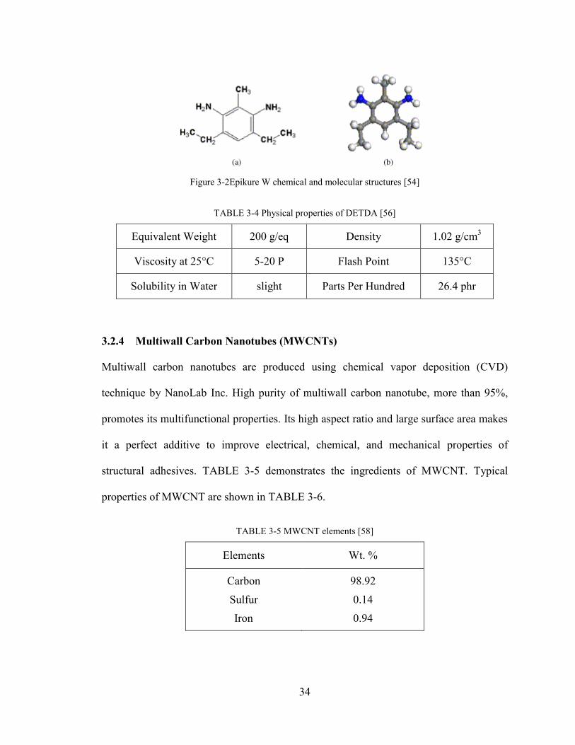
34
Figure 3-2Epikure W chemical and molecular structures [54]
TABLE 3-4 Physical properties of DETDA [56]
Equivalent Weight 200 g/eq Density 1.02 g/cm3
Viscosity at 25°C 5-20 P Flash Point 135°C
Solubility in Water slight Parts Per Hundred 26.4 phr
3.2.4 Multiwall Carbon Nanotubes (MWCNTs)
Multiwall carbon nanotubes are produced using chemical vapor deposition (CVD)
technique by NanoLab Inc. High purity of multiwall carbon nanotube, more than 95%,
promotes its multifunctional properties. Its high aspect ratio and large surface area makes
it a perfect additive to improve electrical, chemical, and mechanical properties of
structural adhesives. TABLE 3-5 demonstrates the ingredients of MWCNT. Typical
properties of MWCNT are shown in TABLE 3-6.
TABLE 3-5 MWCNT elements [58]
Elements Wt. %
Carbon
Sulfur
Iron
98.92
0.14
0.94
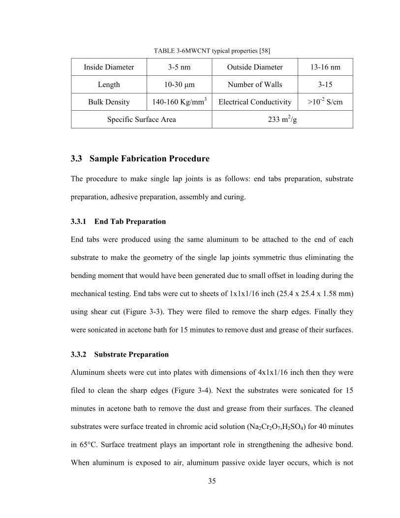
35
TABLE 3-6MWCNT typical properties [58]
Inside Diameter 3-5 nm Outside Diameter 13-16 nm
Length 10-30 μm Number of Walls 3-15
Bulk Density 140-160 Kg/mm3 Electrical Conductivity >10
-2 S/cm
Specific Surface Area 233 m2/g
3.3 Sample Fabrication Procedure
The procedure to make single lap joints is as follows: end tabs preparation, substrate
preparation, adhesive preparation, assembly and curing.
3.3.1 End Tab Preparation
End tabs were produced using the same aluminum to be attached to the end of each
substrate to make the geometry of the single lap joints symmetric thus eliminating the
bending moment that would have been generated due to small offset in loading during the
mechanical testing. End tabs were cut to sheets of 1x1x1/16 inch (25.4 x 25.4 x 1.58 mm)
using shear cut (Figure 3-3). They were filed to remove the sharp edges. Finally they
were sonicated in acetone bath for 15 minutes to remove dust and grease of their surfaces.
3.3.2 Substrate Preparation
Aluminum sheets were cut into plates with dimensions of 4x1x1/16 inch then they were
filed to clean the sharp edges (Figure 3-4). Next the substrates were sonicated for 15
minutes in acetone bath to remove the dust and grease from their surfaces. The cleaned
substrates were surface treated in chromic acid solution (Na2Cr2O7,H2SO4) for 40 minutes
in 65°C. Surface treatment plays an important role in strengthening the adhesive bond.
When aluminum is exposed to air, aluminum passive oxide layer occurs, which is not
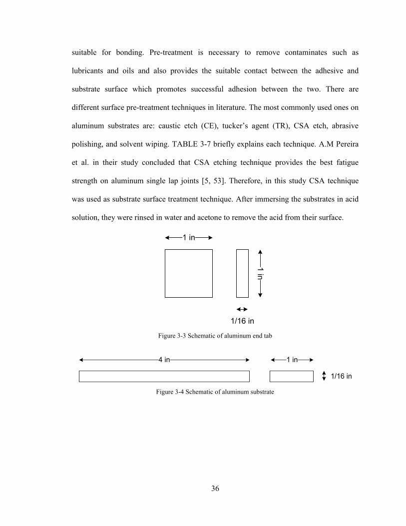
36
suitable for bonding. Pre-treatment is necessary to remove contaminates such as
lubricants and oils and also provides the suitable contact between the adhesive and
substrate surface which promotes successful adhesion between the two. There are
different surface pre-treatment techniques in literature. The most commonly used ones on
aluminum substrates are: caustic etch (CE), tucker’s agent (TR), CSA etch, abrasive
polishing, and solvent wiping. TABLE 3-7 briefly explains each technique. A.M Pereira
et al. in their study concluded that CSA etching technique provides the best fatigue
strength on aluminum single lap joints [5, 53]. Therefore, in this study CSA technique
was used as substrate surface treatment technique. After immersing the substrates in acid
solution, they were rinsed in water and acetone to remove the acid from their surface.
Figure 3-3 Schematic of aluminum end tab
Figure 3-4 Schematic of aluminum substrate
1 in
1 in
1/16 in
4 in 1 in
1/16 in

37
TABLE 3-7 Surface pre-treatment detail [5]
Surface Preparation Technique Procedure
Caustic Etch (CE) Dip specimens in NaOH, H2O
solution for 5-15 min at 60-70 °C,
rinse in water, immerse in HNO3,
rinse in water and dry
Tucker’s Reagent (TR) Dip specimens in HCL, HNO3, HF,
H2O solution for 10-15 min, rinse in
water and dry. This procedure can be
repeated till desired effect is obtained
CSA Immerse specimens in sodium
dichromate-sulphuric acid solution
(650 g H2O distilled, 75 g Na2Cr2O7,
275 g H2SO4) at 60-65 °C. Rinsed in
water and dry.
Abrasive Polishing (AP) The surface is randomly abraded
using P220 grade sandpaper and
cleaned using dry air
Solvent Wiping (SW) Wiping by acetone solvent

38
3.3.3 Adhesive Preparation
Batches of adhesive suspension with different CNT concentrations, namely as 0, 1, 0.5,
and 2 wt% were prepared. Each batch contained weight percentage of MWCNT, of
EPON 862, and of Epicure W which made a mixture of 15 grams. The amount of each
substituent was measured using equations (3-1) to (3-3).
(3-1)
(3-2)
(3-3)
A beaker was weighed on the scale and then the scale was set to zero. MWCNT was
added inside the beaker as required amount measured using the equation. Then the epoxy
was poured inside the beaker and at the end the curing agent was added to the whole
mixture. Since each batch was produced right before being used to make the single lap
joints and the reactivity of the curing agent at room temperature was low, we added the
curing agent to the mixture before dispersing nanotubes inside the adhesive. Therefore
there was no difficulty regarding the shelf time of adhesive suspensions. After adding all
the ingredients, the suspension was mixed using a spatula before it was three-roll milled.
There are different techniques to disperse nanotubes inside adhesive such as, ultrasonic
processing and shear mixing, which includes simple shearing, dissolver disk, planetary
mixer, and three roll milling. Three roll milling technique was chosen to disperse the
nanotube inside the epoxy adhesive since it is solvent free, scalable, and uniformly
applies shear on the entire volume of the suspension [52]. In three-roll milling technique
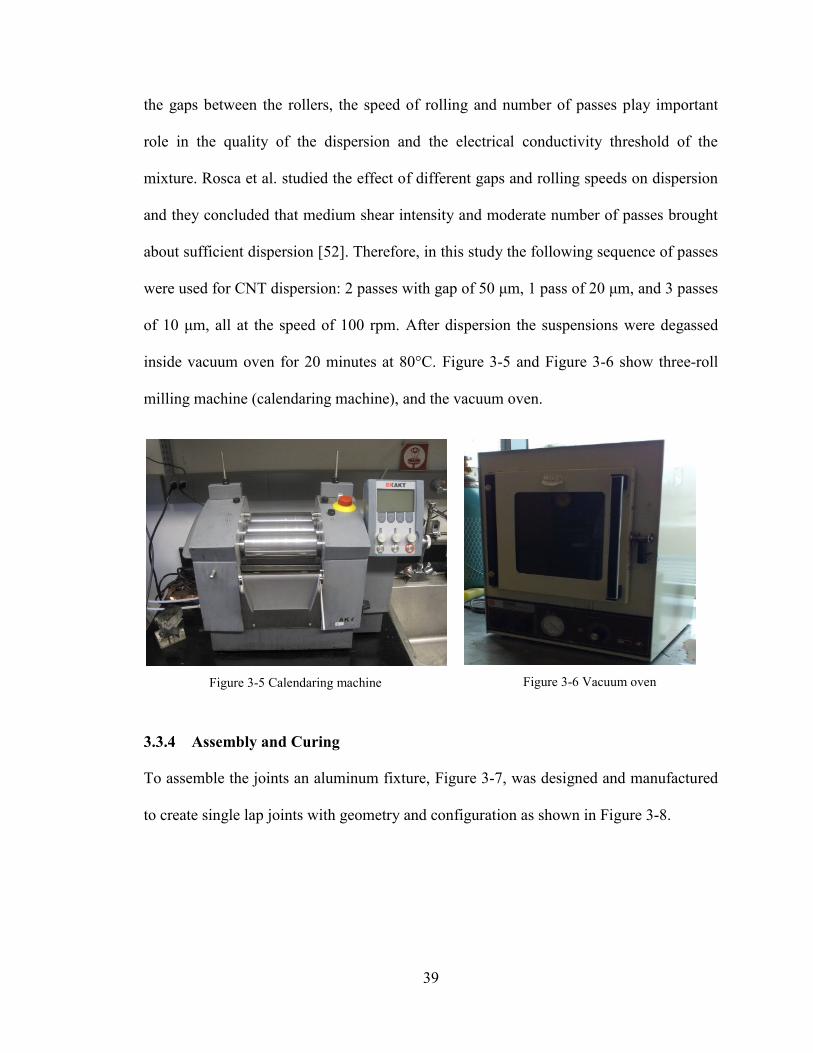
39
the gaps between the rollers, the speed of rolling and number of passes play important
role in the quality of the dispersion and the electrical conductivity threshold of the
mixture. Rosca et al. studied the effect of different gaps and rolling speeds on dispersion
and they concluded that medium shear intensity and moderate number of passes brought
about sufficient dispersion [52]. Therefore, in this study the following sequence of passes
were used for CNT dispersion: 2 passes with gap of 50 μm, 1 pass of 20 μm, and 3 passes
of 10 μm, all at the speed of 100 rpm. After dispersion the suspensions were degassed
inside vacuum oven for 20 minutes at 80°C. Figure 3-5 and Figure 3-6 show three-roll
milling machine (calendaring machine), and the vacuum oven.
Figure 3-5 Calendaring machine
Figure 3-6 Vacuum oven
3.3.4 Assembly and Curing
To assemble the joints an aluminum fixture, Figure 3-7, was designed and manufactured
to create single lap joints with geometry and configuration as shown in Figure 3-8.
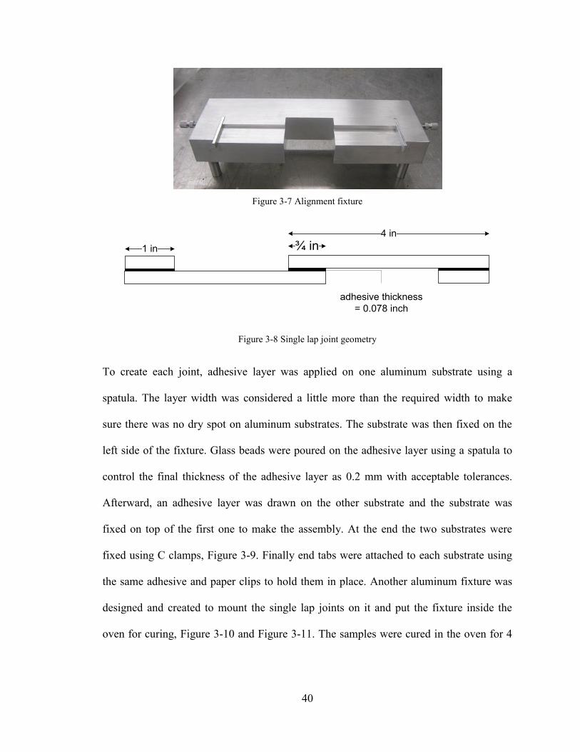
40
Figure 3-7 Alignment fixture
Figure 3-8 Single lap joint geometry
To create each joint, adhesive layer was applied on one aluminum substrate using a
spatula. The layer width was considered a little more than the required width to make
sure there was no dry spot on aluminum substrates. The substrate was then fixed on the
left side of the fixture. Glass beads were poured on the adhesive layer using a spatula to
control the final thickness of the adhesive layer as 0.2 mm with acceptable tolerances.
Afterward, an adhesive layer was drawn on the other substrate and the substrate was
fixed on top of the first one to make the assembly. At the end the two substrates were
fixed using C clamps, Figure 3-9. Finally end tabs were attached to each substrate using
the same adhesive and paper clips to hold them in place. Another aluminum fixture was
designed and created to mount the single lap joints on it and put the fixture inside the
oven for curing, Figure 3-10 and Figure 3-11. The samples were cured in the oven for 4
4 in
¾ in1 in
adhesive thickness
= 0.078 inch

41
hours at 175°C as advised by the resin manufacturer. By each batch of adhesive
suspension, 10 single lap joints were produced for testing.
Figure 3-9 Assembled single lap joint on the fixture
Figure 3-10 Fixture to hold assembled single lap joints inside the oven for curing
Figure 3-11 Assembled samples mounted on the fixture and ready to be cured
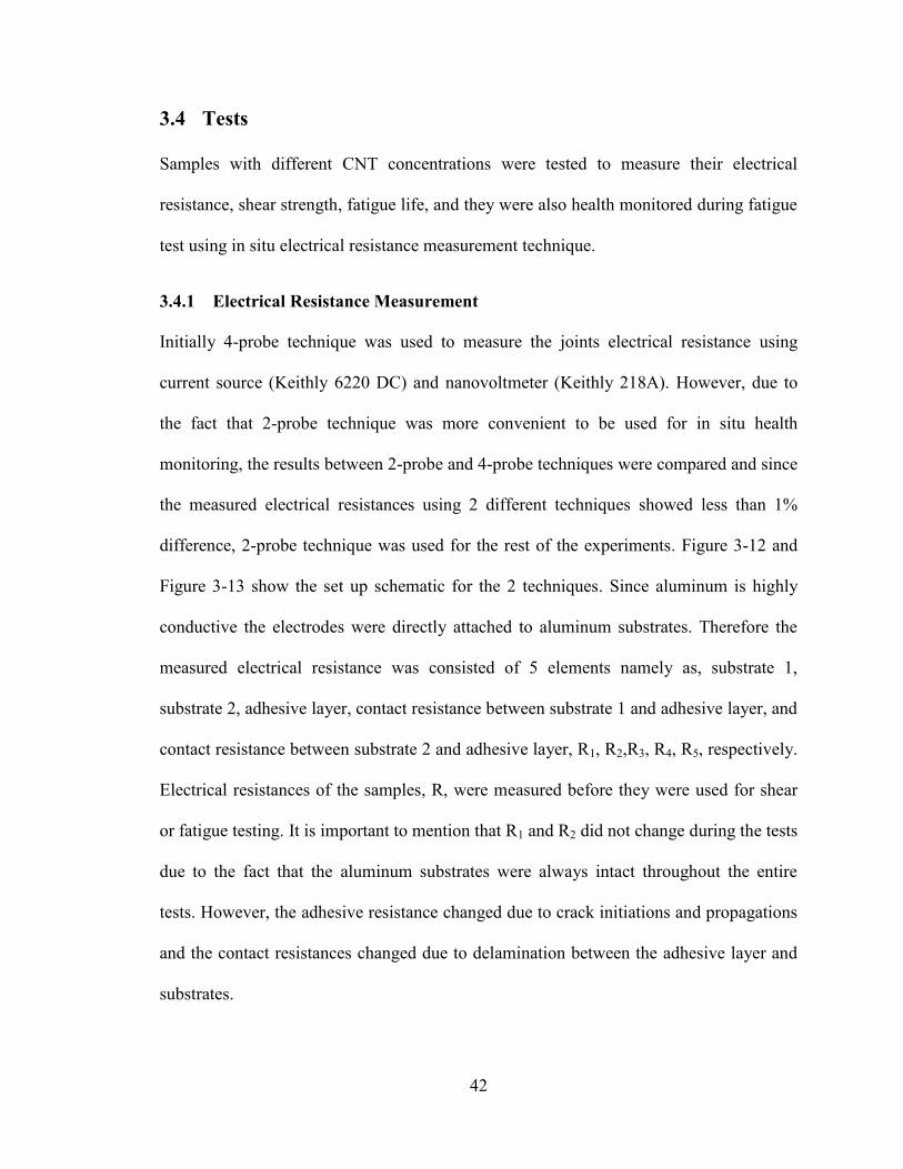
42
3.4 Tests
Samples with different CNT concentrations were tested to measure their electrical
resistance, shear strength, fatigue life, and they were also health monitored during fatigue
test using in situ electrical resistance measurement technique.
3.4.1 Electrical Resistance Measurement
Initially 4-probe technique was used to measure the joints electrical resistance using
current source (Keithly 6220 DC) and nanovoltmeter (Keithly 218A). However, due to
the fact that 2-probe technique was more convenient to be used for in situ health
monitoring, the results between 2-probe and 4-probe techniques were compared and since
the measured electrical resistances using 2 different techniques showed less than 1%
difference, 2-probe technique was used for the rest of the experiments. Figure 3-12 and
Figure 3-13 show the set up schematic for the 2 techniques. Since aluminum is highly
conductive the electrodes were directly attached to aluminum substrates. Therefore the
measured electrical resistance was consisted of 5 elements namely as, substrate 1,
substrate 2, adhesive layer, contact resistance between substrate 1 and adhesive layer, and
contact resistance between substrate 2 and adhesive layer, R1, R2,R3, R4, R5, respectively.
Electrical resistances of the samples, R, were measured before they were used for shear
or fatigue testing. It is important to mention that R1 and R2 did not change during the tests
due to the fact that the aluminum substrates were always intact throughout the entire
tests. However, the adhesive resistance changed due to crack initiations and propagations
and the contact resistances changed due to delamination between the adhesive layer and
substrates.
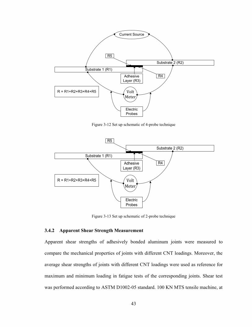
43
Figure 3-12 Set up schematic of 4-probe technique
Figure 3-13 Set up schematic of 2-probe technique
3.4.2 Apparent Shear Strength Measurement
Apparent shear strengths of adhesively bonded aluminum joints were measured to
compare the mechanical properties of joints with different CNT loadings. Moreover, the
average shear strengths of joints with different CNT loadings were used as reference for
maximum and minimum loading in fatigue tests of the corresponding joints. Shear test
was performed according to ASTM D1002-05 standard. 100 KN MTS tensile machine, at
Substrate 1 (R1)
Substrate 2 (R2)
VoltMeter
Adhesive
Layer (R3)
Electric
Probes
R = R1+R2+R3+R4+R5
R5
R4
Current Source
Substrate 1 (R1)
Substrate 2 (R2)
VoltMeter
Adhesive
Layer (R3)
Electric
Probes
R = R1+R2+R3+R4+R5
R5
R4
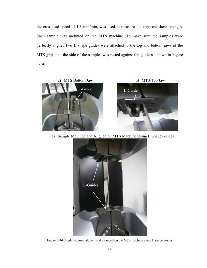
44
the crosshead speed of 1.3 mm/min, was used to measure the apparent shear strength.
Each sample was mounted on the MTS machine. To make sure the samples were
perfectly aligned two L shape guides were attached to the top and bottom jaws of the
MTS grips and the side of the samples was rested against the guide as shown in Figure
3-14.
a) MTS Bottom Jaw
b) MTS Top Jaw
c) Sample Mounted and Aligned on MTS Machine Using L Shape Guides
Figure 3-14 Single lap joint aligned and mounted on the MTS machine using L shape guides
L-Guide L-Guide
L-Guides
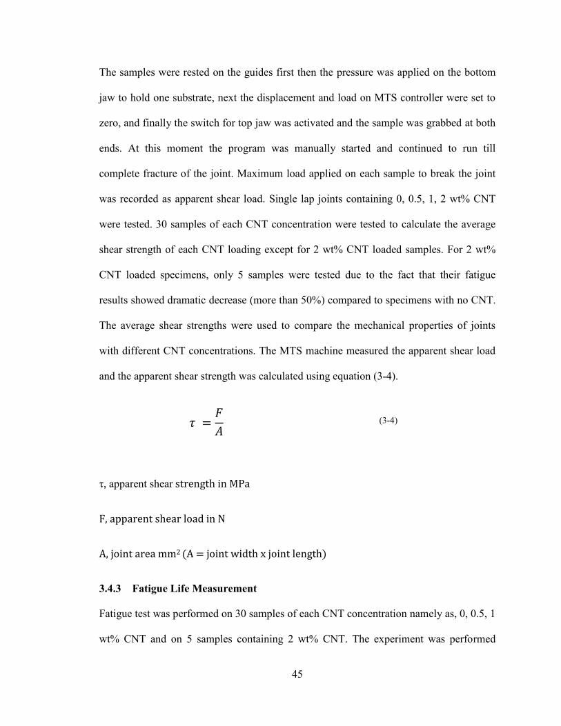
45
The samples were rested on the guides first then the pressure was applied on the bottom
jaw to hold one substrate, next the displacement and load on MTS controller were set to
zero, and finally the switch for top jaw was activated and the sample was grabbed at both
ends. At this moment the program was manually started and continued to run till
complete fracture of the joint. Maximum load applied on each sample to break the joint
was recorded as apparent shear load. Single lap joints containing 0, 0.5, 1, 2 wt% CNT
were tested. 30 samples of each CNT concentration were tested to calculate the average
shear strength of each CNT loading except for 2 wt% CNT loaded samples. For 2 wt%
CNT loaded specimens, only 5 samples were tested due to the fact that their fatigue
results showed dramatic decrease (more than 50%) compared to specimens with no CNT.
The average shear strengths were used to compare the mechanical properties of joints
with different CNT concentrations. The MTS machine measured the apparent shear load
and the apparent shear strength was calculated using equation (3-4).
(3-4)
τ, apparent shear strength in MPa
F, apparent shear load in N
A, joint area mm2 (A = joint width x joint length)
3.4.3 Fatigue Life Measurement
Fatigue test was performed on 30 samples of each CNT concentration namely as, 0, 0.5, 1
wt% CNT and on 5 samples containing 2 wt% CNT. The experiment was performed

46
according to ASTM D3166-99 standard. Maximum load σmax, was set at 60% of the
average shear load measured from shear test to expedite the fatigue test since lower
maximum fatigue load would result in excessive time required to finish the tests. The
ratio of 0.1 was used to measure minimum load σmin, according to the standard. The 100
KN MTS tensile machine was used to do the fatigue tests. The procedure to mount the
samples on the MTS machine was the same as described in previous section. All tests
were performed at 10 Hz until final failure occurred. The fatigue cycle in which the joint
was broken was recorded as fatigue life of that joint.
3.4.4 In-Situ Health Monitoring of Single Lap Joints during Fatigue Test
The state of the samples was monitored using electrical resistance measurement
technique, while they were being fatigue tested. After mounting the sample on the MTS
machine, electrical probes connected to the nanovoltmeter, were attached to each
substrate. The voltmeter was connected to the data acquisition system to record and to
save the joint electrical resistance at every second till its final failure. The results were
plotted on an excel sheet as resistance vs. time. The electrical probes were directly
attached to the aluminum substrates rather than being inserted inside the adhesive. This is
because it was more convenient; it was not degrading the mechanical properties of the
joints unlike in the case of inserting wire; and more importantly it was possible to
measure the contact electrical resistances between the adhesive layer and each substrate.
The contact resistances were of great importance in monitoring the health of the joints
especially at the final stages of their fatigue lives. Figure 3-15 shows the in-situ health
monitoring set-up.
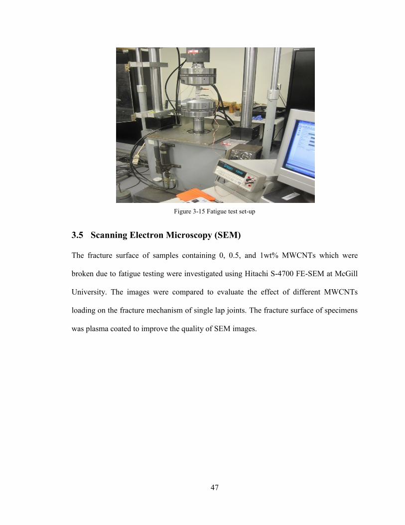
47
Figure 3-15 Fatigue test set-up
3.5 Scanning Electron Microscopy (SEM)
The fracture surface of samples containing 0, 0.5, and 1wt% MWCNTs which were
broken due to fatigue testing were investigated using Hitachi S-4700 FE-SEM at McGill
University. The images were compared to evaluate the effect of different MWCNTs
loading on the fracture mechanism of single lap joints. The fracture surface of specimens
was plasma coated to improve the quality of SEM images.

48
Chapter 4
Results and
Discussions
49
4 Results and Discussions
4.1 Introduction
The main focus of this study was in-situ health monitoring of adhesively bonded joints
during fatigue life. Therefore, fatigue test is the prime experiment to evaluate our
technique. However, preliminary testing is required to perform fatigue test. Shear
strength test was performed first to assess the maximum shear load required to break the
samples. The average shear load is then used to calculate the loading required for fatigue
testing. Moreover, since introduction of MWCNTs would change the electromechanical
properties of adhesive joints, it was important to compare the electromechanical
properties of the joints containing MWCNTs with different wt. % to each other and to the
joints with neat adhesive as the reference. This chapter provides detail results and
discussions for each experiment.
4.2 Electrical resistance
The test set-up and technique to measure the electrical resistance were explained in
section3.4.1. All sample electrical resistances except for the joints with neat epoxy
adhesive were measured and recorded. The results for 0.5 and 1 wt% CNT reinforced
adhesive joints were compared to each other. However, due to fewer numbers of
specimens for 2 wt% CNT loading, the result for specimens containing 2 wt% CNT is
presented separately.
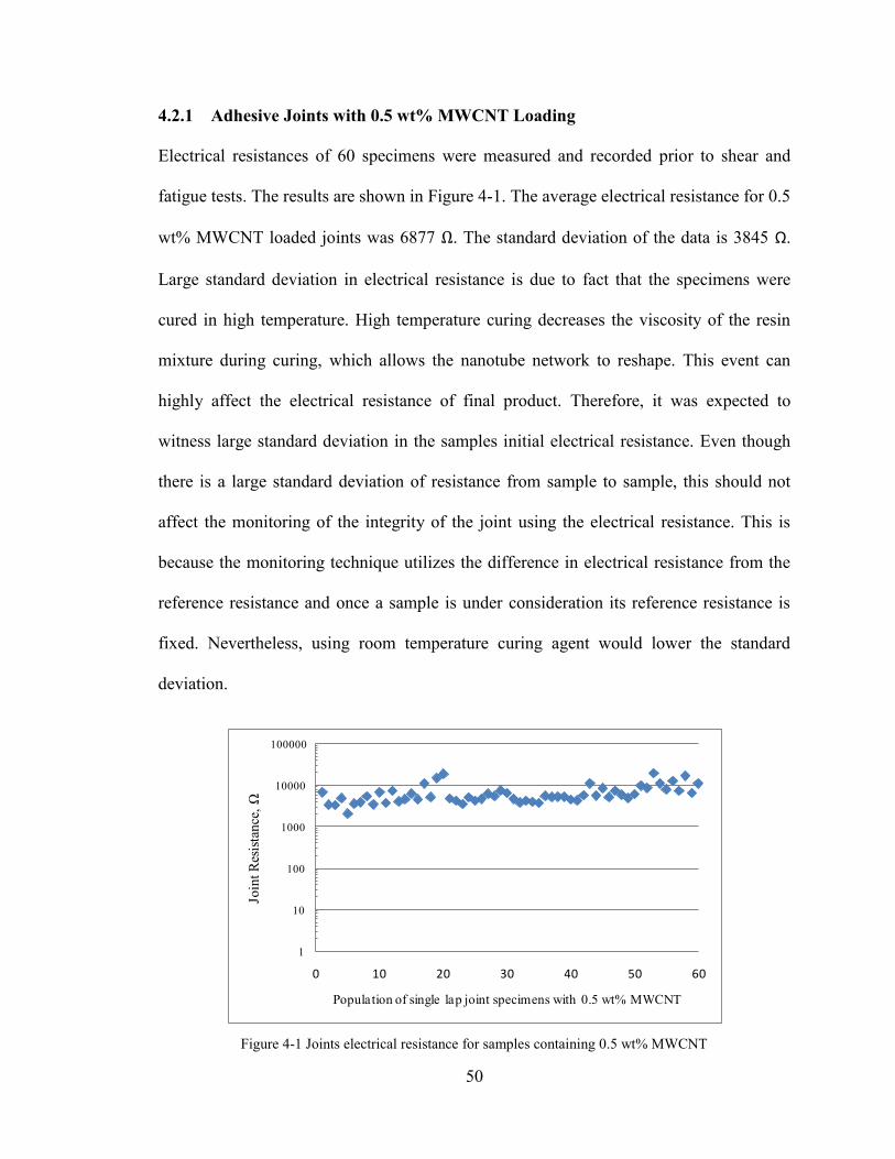
50
4.2.1 Adhesive Joints with 0.5 wt% MWCNT Loading
Electrical resistances of 60 specimens were measured and recorded prior to shear and
fatigue tests. The results are shown in Figure 4-1. The average electrical resistance for 0.5
wt% MWCNT loaded joints was 6877 Ω. The standard deviation of the data is 3845 Ω.
Large standard deviation in electrical resistance is due to fact that the specimens were
cured in high temperature. High temperature curing decreases the viscosity of the resin
mixture during curing, which allows the nanotube network to reshape. This event can
highly affect the electrical resistance of final product. Therefore, it was expected to
witness large standard deviation in the samples initial electrical resistance. Even though
there is a large standard deviation of resistance from sample to sample, this should not
affect the monitoring of the integrity of the joint using the electrical resistance. This is
because the monitoring technique utilizes the difference in electrical resistance from the
reference resistance and once a sample is under consideration its reference resistance is
fixed. Nevertheless, using room temperature curing agent would lower the standard
deviation.
Figure 4-1 Joints electrical resistance for samples containing 0.5 wt% MWCNT
1
10
100
1000
10000
100000
0 10 20 30 40 50 60
Join
t R
esis
tance
, Ω
Population of single lap joint specimens with 0.5 wt% MWCNT

51
4.2.2 Adhesive Joints with 1 wt% MWCNT Loading
Electrical resistances of 60 specimens were measured and recorded prior to shear and
fatigue tests. The results are shown in Figure 4-2. The average electrical resistance for
1wt% MWCNT loaded joints was 550 Ω. The standard deviation for the data is 451 Ω.
The same fact as described in section 4.2.1 can explain high standard deviation in the
case of 1 wt% MWCNTs loading.
Figure 4-2 Joints electrical resistance for samples containing 1wt% MWCNT
4.2.3 Comparison
Figure 4-3 shows the comparison between the electrical resistance of single lap joints
containing 0.5 and 1 wt% MWCNT.
1
10
100
1000
10000
0 10 20 30 40 50 60
Join
t R
esi
sta
nce, Ω
Population of single lap joint speciments with 1 wt% MWCNT
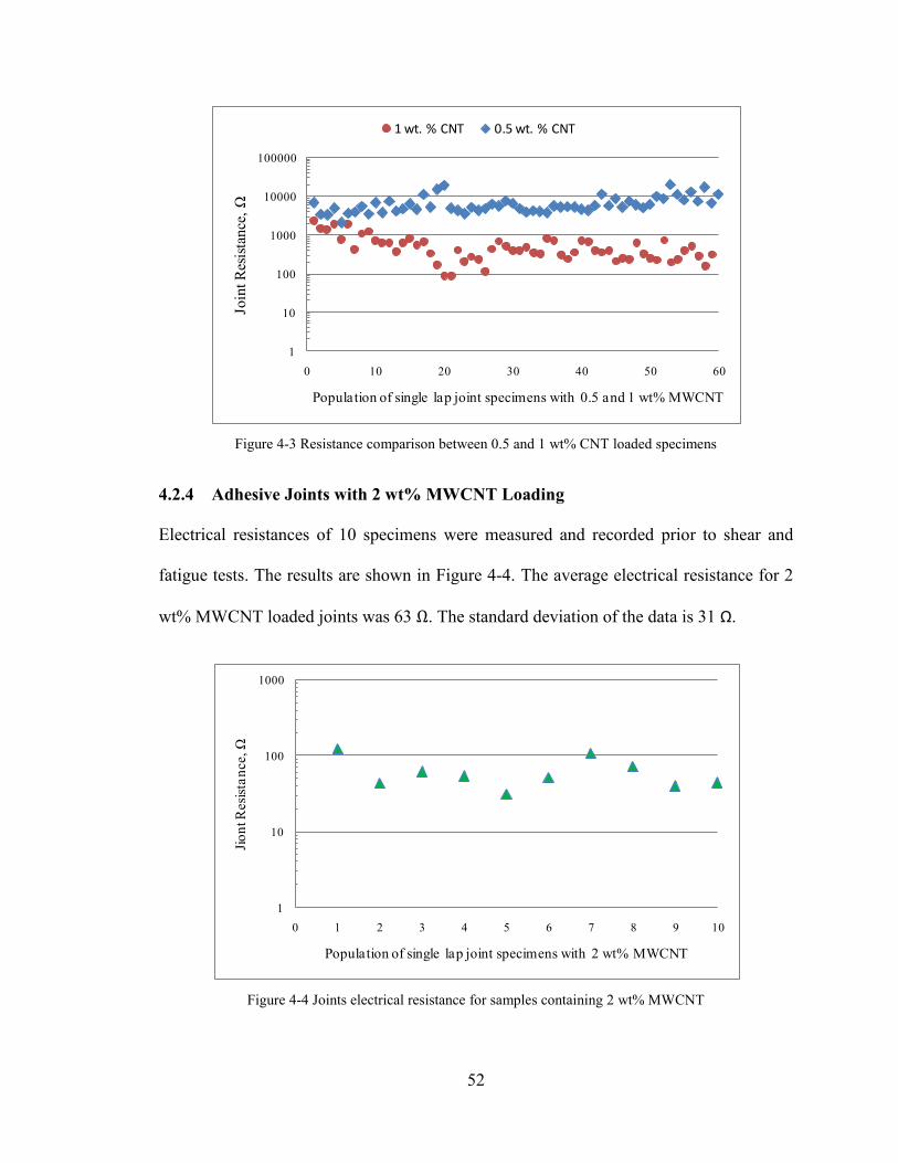
52
Figure 4-3 Resistance comparison between 0.5 and 1 wt% CNT loaded specimens
4.2.4 Adhesive Joints with 2 wt% MWCNT Loading
Electrical resistances of 10 specimens were measured and recorded prior to shear and
fatigue tests. The results are shown in Figure 4-4. The average electrical resistance for 2
wt% MWCNT loaded joints was 63 Ω. The standard deviation of the data is 31 Ω.
Figure 4-4 Joints electrical resistance for samples containing 2 wt% MWCNT
1
10
100
1000
10000
100000
0 10 20 30 40 50 60
Join
t R
esis
tan
ce,
Ω
Population of single lap joint specimens with 0.5 and 1 wt% MWCNT
1 wt. % CNT 0.5 wt. % CNT
1
10
100
1000
0 1 2 3 4 5 6 7 8 9 10
Jio
nt R
esi
sta
nce, Ω
Population of single lap joint specimens with 2 wt% MWCNT

53
4.2.5 Summary
Joint with neat adhesive has resistance of 5x10¹¹
Ω. Adding 0.5 and 1 wt% of MWCNT
decreased the resistance 7 and 8 orders of magnitude to 6877 Ω and 550 Ω respectively.
By adding 2 wt% of MWCNT the resistance reduces 10 orders of magnitude to 63
Ω.Therefore, the addition of MWCNT inside adhesive improved the electrical properties
of the joints. Figure 4-5 shows the comparison between the average electrical resistances
of the joints containing different concentrations of MWCNTs.

54
Figure 4-5 Average electrical resistance comparison between the joints containing 0, 0.5, 1, and 2 wt% MWCNT
1
10
100
1000
10000R
esis
tan
ce, Ω
0.5 wt% CNT 1 wt% CNT 2 wt% CNT
R0 wt% CNT = 5x10¹¹ Ω
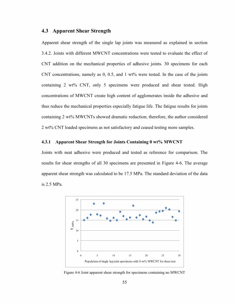
55
4.3 Apparent Shear Strength
Apparent shear strength of the single lap joints was measured as explained in section
3.4.2. Joints with different MWCNT concentrations were tested to evaluate the effect of
CNT addition on the mechanical properties of adhesive joints. 30 specimens for each
CNT concentrations, namely as 0, 0.5, and 1 wt% were tested. In the case of the joints
containing 2 wt% CNT, only 5 specimens were produced and shear tested. High
concentrations of MWCNT create high content of agglomerates inside the adhesive and
thus reduce the mechanical properties especially fatigue life. The fatigue results for joints
containing 2 wt% MWCNTs showed dramatic reduction; therefore, the author considered
2 wt% CNT loaded specimens as not satisfactory and ceased testing more samples.
4.3.1 Apparent Shear Strength for Joints Containing 0 wt% MWCNT
Joints with neat adhesive were produced and tested as reference for comparison. The
results for shear strengths of all 30 specimens are presented in Figure 4-6. The average
apparent shear strength was calculated to be 17.5 MPa. The standard deviation of the data
is 2.5 MPa.
Figure 4-6 Joint apparent shear strength for specimens containing no MWCNT
0
5
10
15
20
25
0 5 10 15 20 25 30
τ, M
Pa
Population of single lap joint specimens with 0 wt% MWCNT for shear test

56
4.3.2 Apparent Shear Strength for Joints Containing 0.5 wt% MWCNT
The apparent shear strengths of all 30 specimens containing 0.5 wt% MWCNT are
presented in Figure 4-7. The average shear strength was calculated to be 19.6 MPa. The
standard deviation of the data is 2.3 MPa. Since it was assumed that there would be a
correlation between the joints initial resistance and final shear strength, the shear
strengths of the joints were plotted versus initial electrical resistances ordered from the
lowest resistance to the highest resistance and shown in Figure 4-8. However, on the
contrary to the assumption, the results clearly indicate that there is no correlation between
the initial resistance and the shear strength of the joints. Therefore, it is not possible to
evaluate the quality of the joints only by measuring the initial electrical resistance prior to
testing.
Figure 4-7Joint apparent shear strength for specimens containing 0.5 wt% MWCNT
0
5
10
15
20
25
30
0 5 10 15 20 25 30
τ, M
Pa
Population of single lap joint specimens with 0.5 wt% MWCNT for shear test

57
Figure 4-8 Shear strength vs. electrical resistance for single lap joints containing 0.5 wt% MWCNT
4.3.3 Apparent Shear Strength for Joints Containing 1 wt% MWCNT
Figure 4-9 shows the apparent shear strengths of all 30 specimens containing 1 wt%
MWCNT. The average shear strength of the joints was 19 MPa. The standard deviation
of the data is 2.3 MPa. Figure 4-10 shows the shear strength versus electrical resistance
ordered from the lowest resistance to the highest resistance. As it is clear from the figure
there is no correlation between the electrical resistance and shear strength of the joints
containing 1 wt% MWCNT.
Figure 4-9 Joint apparent shear strength for specimens containing 1 wt% MWCNT
0
5
10
15
20
25
30
0 5000 10000 15000 20000 25000
τ , M
Pa
Resistance, Ω
0
5
10
15
20
25
30
0 5 10 15 20 25 30
τ, M
Pa
Population of single lap joint specimens with 1 wt% MWCNT for shear test
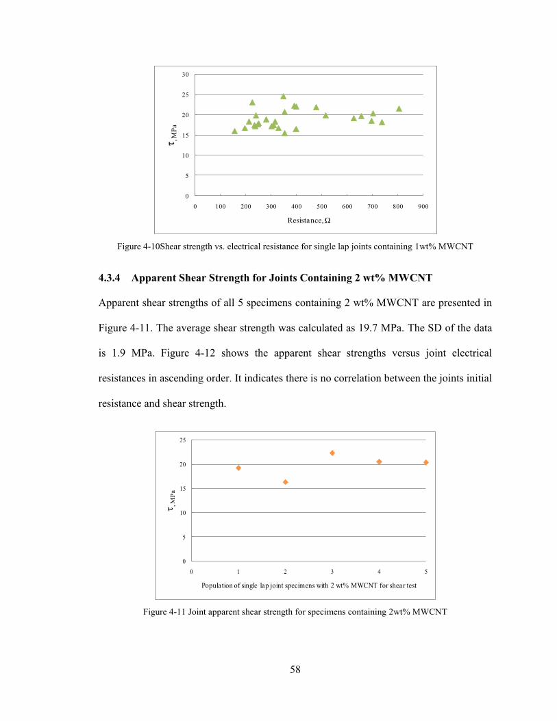
58
Figure 4-10Shear strength vs. electrical resistance for single lap joints containing 1wt% MWCNT
4.3.4 Apparent Shear Strength for Joints Containing 2 wt% MWCNT
Apparent shear strengths of all 5 specimens containing 2 wt% MWCNT are presented in
Figure 4-11. The average shear strength was calculated as 19.7 MPa. The SD of the data
is 1.9 MPa. Figure 4-12 shows the apparent shear strengths versus joint electrical
resistances in ascending order. It indicates there is no correlation between the joints initial
resistance and shear strength.
Figure 4-11 Joint apparent shear strength for specimens containing 2wt% MWCNT
0
5
10
15
20
25
30
0 100 200 300 400 500 600 700 800 900
τ , M
Pa
Resistance, Ω
0
5
10
15
20
25
0 1 2 3 4 5
τ, M
Pa
Population of single lap joint specimens with 2 wt% MWCNT for shear test

59
Figure 4-12Shear strength vs. electrical resistance for single lap joints containing 2wt% MWCNT
4.3.5 Comparison
Figure 4-13 shows the comparison between the average shear strengths of single lap
joints containing 0, 0.5, 1, and 2 wt% MWCNT.
Figure 4-13 Average shear strength comparison between the joints containing 0, 0.5, 1, and 2 wt%
MWCNT
0
5
10
15
20
25
0 20 40 60 80 100 120
τ , M
Pa
Resistance, Ω
0
5
10
15
20
25
τ , M
Pa
0 wt% CNT 0.5 wt% CNT 1 wt% CNT 2 wt% CNT
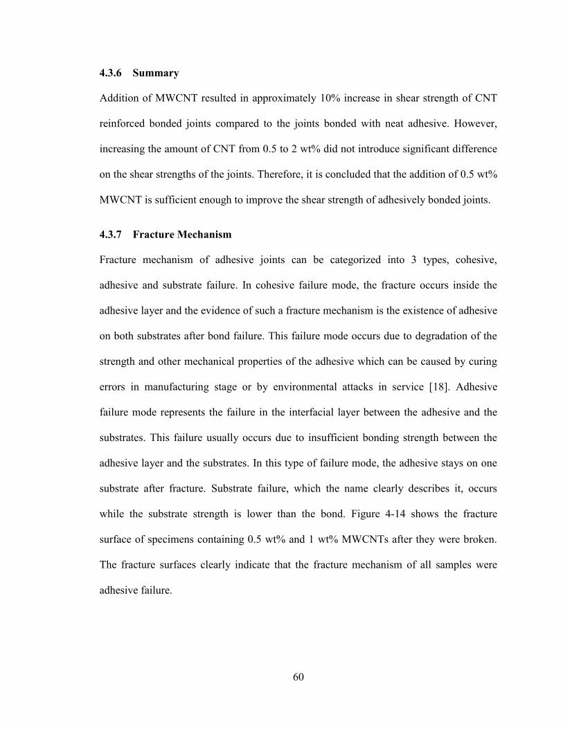
60
4.3.6 Summary
Addition of MWCNT resulted in approximately 10% increase in shear strength of CNT
reinforced bonded joints compared to the joints bonded with neat adhesive. However,
increasing the amount of CNT from 0.5 to 2 wt% did not introduce significant difference
on the shear strengths of the joints. Therefore, it is concluded that the addition of 0.5 wt%
MWCNT is sufficient enough to improve the shear strength of adhesively bonded joints.
4.3.7 Fracture Mechanism
Fracture mechanism of adhesive joints can be categorized into 3 types, cohesive,
adhesive and substrate failure. In cohesive failure mode, the fracture occurs inside the
adhesive layer and the evidence of such a fracture mechanism is the existence of adhesive
on both substrates after bond failure. This failure mode occurs due to degradation of the
strength and other mechanical properties of the adhesive which can be caused by curing
errors in manufacturing stage or by environmental attacks in service [18]. Adhesive
failure mode represents the failure in the interfacial layer between the adhesive and the
substrates. This failure usually occurs due to insufficient bonding strength between the
adhesive layer and the substrates. In this type of failure mode, the adhesive stays on one
substrate after fracture. Substrate failure, which the name clearly describes it, occurs
while the substrate strength is lower than the bond. Figure 4-14 shows the fracture
surface of specimens containing 0.5 wt% and 1 wt% MWCNTs after they were broken.
The fracture surfaces clearly indicate that the fracture mechanism of all samples were
adhesive failure.
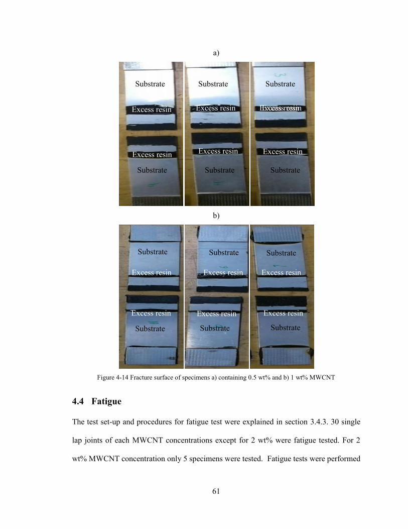
61
a)
b)
Figure 4-14 Fracture surface of specimens a) containing 0.5 wt% and b) 1 wt% MWCNT
4.4 Fatigue
The test set-up and procedures for fatigue test were explained in section 3.4.3. 30 single
lap joints of each MWCNT concentrations except for 2 wt% were fatigue tested. For 2
wt% MWCNT concentration only 5 specimens were tested. Fatigue tests were performed
Substrate Substrate Substrate
Substrate Substrate Substrate
Excess resin Excess resin Excess resin
Excess resin Excess resin Excess resin
Substrate Substrate Substrate
Substrate Substrate Substrate
Excess resin Excess resin Excess resin
Excess resin Excess resin Excess resin
Excess resin
62
on the specimens based on two objectives, 1) to compare the fatigue life of single lap
joints containing different percentages of CNT 2) to evaluate the state of the joints during
their fatigue life by using electrical resistance technique. Since the addition of MWCNTs
to the adhesive was a requirement for our in-situ health monitoring technique, it was
important to make sure that their addition would not deteriorate the fatigue life of the
adhesive joints. Therefore, this section explains the results achieved for the first
objective.
4.4.1 Fatigue Life for Single Lap Joints Containing No MWCNTs
Single lap joints with neat epoxy adhesive were fatigue tested. The results were used as
reference for comparison. The maximum load was set at 60% of the average shear load.
The average shear load for samples with neat epoxy was 8300 N thus the maximum load
was set to 5000 N. The ratio between the max loading and min loading was 0.1 hence the
min load was set to 500 N. Figure 4-15 shows the fatigue life of all 30 single lap joints
with no MWCNTs. Fatigue results usually have large scatter due to the complexity of the
test itself, therefore, the fatigue life distribution is shown in Figure 4-16. The average
fatigue life of the joints with 0 wt% MWCNT was calculated as the average of the fatigue
lives of all 30 specimens tested and it was 20,900 cycles. The failure mechanism was
observed to be mainly adhesive. Figure 4-17 shows the fracture surface of a single lap
joint with no MWCNTs which was broken due to fatigue loading. Multiple cracks are
also visible in the image.

63
Figure 4-15 Single lap joint fatigue life for specimens containing 0 wt% MWCNT
Figure 4-16 Single lap joints fatigue life distributions for specimens with 0 wt% MWCNT
0
10000
20000
30000
40000
50000
60000
70000
0 5 10 15 20 25 30
No
. o
f cy
cle
s to
fail
ure
Population of single lap joint specimens with 0 wt% MWCNT for fatigue test
0
5
10
15
20
25
30
35
40
0-10 10-20 20-30 30-40 40-50 50-60 more
Dis
trib
uti
on
%
Fatigue failure cycle x1000

64
Figure 4-17 SEM image of a fracture surface of a sample containing no MWCNTs after the sample was
broken due to fatigue loading
X
Y
X
Interface Layer
Adhesive Layer
Glass Beads
B
A
A
B
65
4.4.2 Fatigue Life for Single Lap Joints Containing 0.5 wt% MWCNTs
30 specimens containing 0.5 wt% MWCNT were fatigue tested. The maximum loading
for fatigue tests was set as 5700 N corresponding to 60% of the average shear load, 9500
N, calculated in shear tests. The minimum load for fatigue test was set as 570, 10% of the
maximum load. Figure 4-18 displays the fatigue life of all 30 samples containing 0.5 wt%
MWCNT. The fatigue life distribution is shown in Figure 4-19.
Figure 4-18 Single lap joint fatigue life for specimens containing 0.5wt% MWCNT
Figure 4-19 Single lap joints fatigue life distributions for specimens with 0.5 wt% MWCNT
0
10000
20000
30000
40000
50000
60000
70000
80000
90000
0 5 10 15 20 25 30
No
. o
f cy
cle
s to
fail
ure
Population of single lap joint specimens with 0.5 wt% MWCNT for fatigue test
0
5
10
15
20
25
30
35
40
0-10 10-20 20-30 30-40 40-50 50-60 more
Dis
trib
uti
on %
Fatigue failure cycle x1000
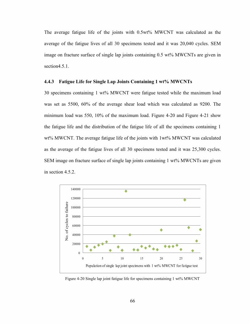
66
The average fatigue life of the joints with 0.5wt% MWCNT was calculated as the
average of the fatigue lives of all 30 specimens tested and it was 20,040 cycles. SEM
image on fracture surface of single lap joints containing 0.5 wt% MWCNTs are given in
section4.5.1.
4.4.3 Fatigue Life for Single Lap Joints Containing 1 wt% MWCNTs
30 specimens containing 1 wt% MWCNT were fatigue tested while the maximum load
was set as 5500, 60% of the average shear load which was calculated as 9200. The
minimum load was 550, 10% of the maximum load. Figure 4-20 and Figure 4-21 show
the fatigue life and the distribution of the fatigue life of all the specimens containing 1
wt% MWCNT. The average fatigue life of the joints with 1wt% MWCNT was calculated
as the average of the fatigue lives of all 30 specimens tested and it was 25,300 cycles.
SEM image on fracture surface of single lap joints containing 1 wt% MWCNTs are given
in section 4.5.2.
Figure 4-20 Single lap joint fatigue life for specimens containing 1 wt% MWCNT
0
20000
40000
60000
80000
100000
120000
140000
0 5 10 15 20 25 30
No
. o
f cy
cle
s to
fail
ure
Population of single lap joint specimens with 1 wt% MWCNT for fatigue test
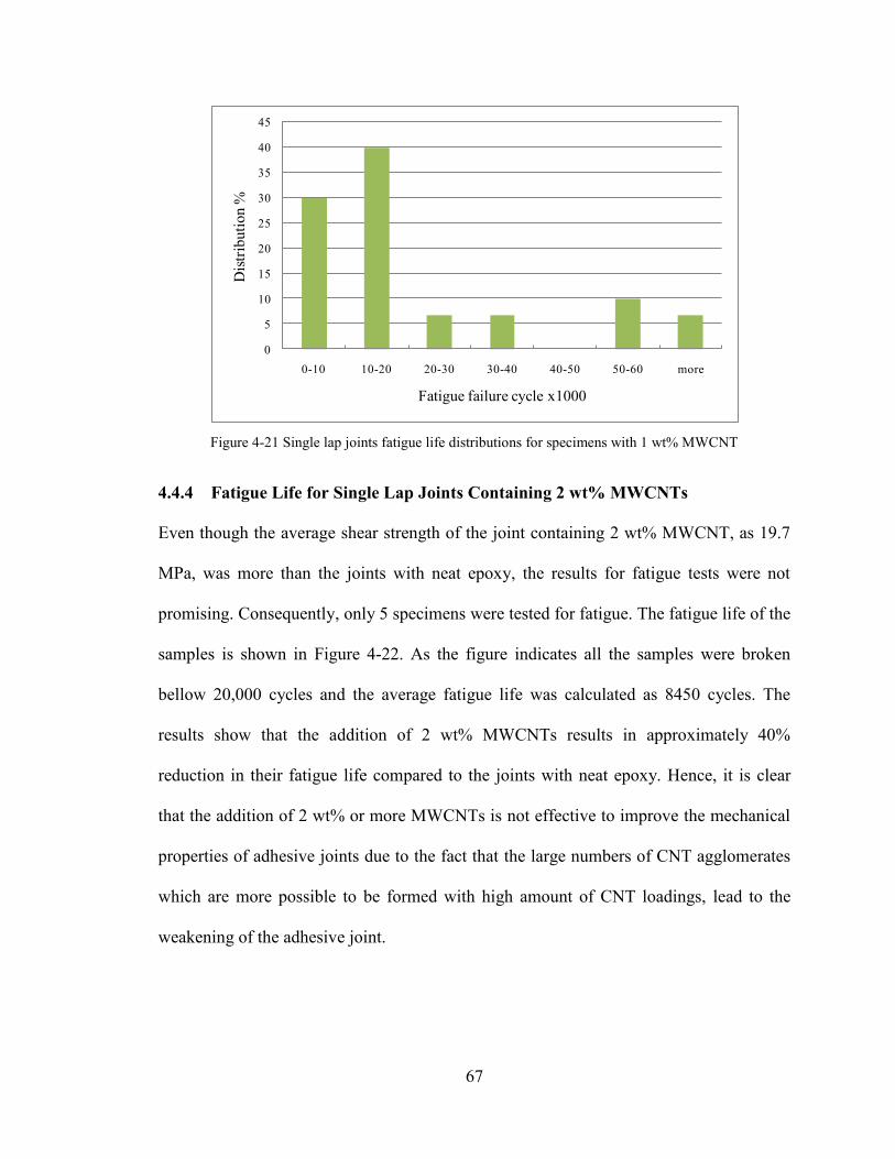
67
Figure 4-21 Single lap joints fatigue life distributions for specimens with 1 wt% MWCNT
4.4.4 Fatigue Life for Single Lap Joints Containing 2 wt% MWCNTs
Even though the average shear strength of the joint containing 2 wt% MWCNT, as 19.7
MPa, was more than the joints with neat epoxy, the results for fatigue tests were not
promising. Consequently, only 5 specimens were tested for fatigue. The fatigue life of the
samples is shown in Figure 4-22. As the figure indicates all the samples were broken
bellow 20,000 cycles and the average fatigue life was calculated as 8450 cycles. The
results show that the addition of 2 wt% MWCNTs results in approximately 40%
reduction in their fatigue life compared to the joints with neat epoxy. Hence, it is clear
that the addition of 2 wt% or more MWCNTs is not effective to improve the mechanical
properties of adhesive joints due to the fact that the large numbers of CNT agglomerates
which are more possible to be formed with high amount of CNT loadings, lead to the
weakening of the adhesive joint.
0
5
10
15
20
25
30
35
40
45
0-10 10-20 20-30 30-40 40-50 50-60 more
Dis
trib
uti
on
%
Fatigue failure cycle x1000
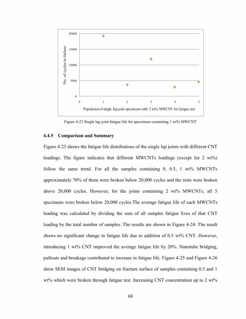
68
Figure 4-22 Single lap joint fatigue life for specimens containing 1 wt% MWCNT
4.4.5 Comparison and Summary
Figure 4-23 shows the fatigue life distributions of the single lap joints with different CNT
loadings. The figure indicates that different MWCNTs loadings (except for 2 wt%)
follow the same trend. For all the samples containing 0, 0.5, 1 wt% MWCNTs
approximately 70% of them were broken below 20,000 cycles and the rests were broken
above 20,000 cycles. However, for the joints containing 2 wt% MWCNTs, all 5
specimens were broken below 20,000 cycles.The average fatigue life of each MWCNTs
loading was calculated by dividing the sum of all samples fatigue lives of that CNT
loading by the total number of samples. The results are shown in Figure 4-24. The result
shows no significant change in fatigue life due to addition of 0.5 wt% CNT. However,
introducing 1 wt% CNT improved the average fatigue life by 20%. Nanotube bridging,
pullouts and breakage contributed to increase in fatigue life. Figure 4-25 and Figure 4-26
show SEM images of CNT bridging on fracture surface of samples containing 0.5 and 1
wt% which were broken through fatigue test. Increasing CNT concentration up to 2 wt%
0
5000
10000
15000
20000
0 1 2 3 4 5
No
. o
f cy
cle
s to
fail
ure
Population of single lap joint specimens with 2 wt% MWCNT for fatigue test
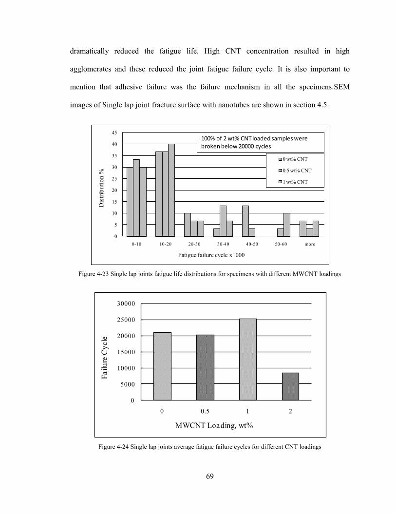
69
dramatically reduced the fatigue life. High CNT concentration resulted in high
agglomerates and these reduced the joint fatigue failure cycle. It is also important to
mention that adhesive failure was the failure mechanism in all the specimens.SEM
images of Single lap joint fracture surface with nanotubes are shown in section 4.5.
Figure 4-23 Single lap joints fatigue life distributions for specimens with different MWCNT loadings
Figure 4-24 Single lap joints average fatigue failure cycles for different CNT loadings
0
5
10
15
20
25
30
35
40
45
0-10 10-20 20-30 30-40 40-50 50-60 more
Dis
trib
uti
on
%
Fatigue failure cycle x1000
0 wt% CNT
0.5 wt% CNT
1 wt% CNT
100% of 2 wt% CNT loaded samples were broken below 20000 cycles
0
5000
10000
15000
20000
25000
30000
0 0.5 1 2
Fa
ilu
re C
ycle
MWCNT Loading, wt%

70
a)
b)
c)
d)
Figure 4-25 SEM images of fracture surface of a samples containing 0.5wt% MWCNT showing CNT
bridging in different magnifications a) shows the fracture surface and b, c, and d show magnified images
Load
Direction Excess Resin

71
a)
b) c)
d) e) Figure 4-26 SEM images of fracture surface of a samples containing 1 wt% MWCNT showing CNT
bridging in different magnifications a) shows the fracture surface and b, c, d and e show magnified images
4.5 In situ Health Monitoring during Fatigue Test
The electrical resistance signatures of all the samples that were fatigue tested were
recorded during the tests. The change in resistance from the initial joint resistance was
used as a reference to evaluate the state of the joint. It was assumed that the increase in
resistance would occur while cracks initiated and propagated and continued to increase
dramatically till the final failure of the joint.
4.5.1 Single lap joints containing 0.5 wt% MWCNT
Figure 4-27 to Figure 4-36 show 5 examples of electrical resistance signature and
electrical resistance ratio of the joints containing 0.5 wt% MWCNTs. The electrical
resistance signatures and ratios for all the specimens are shown in Appendix I. Each
Load Direction
Load Direction
Excess resin
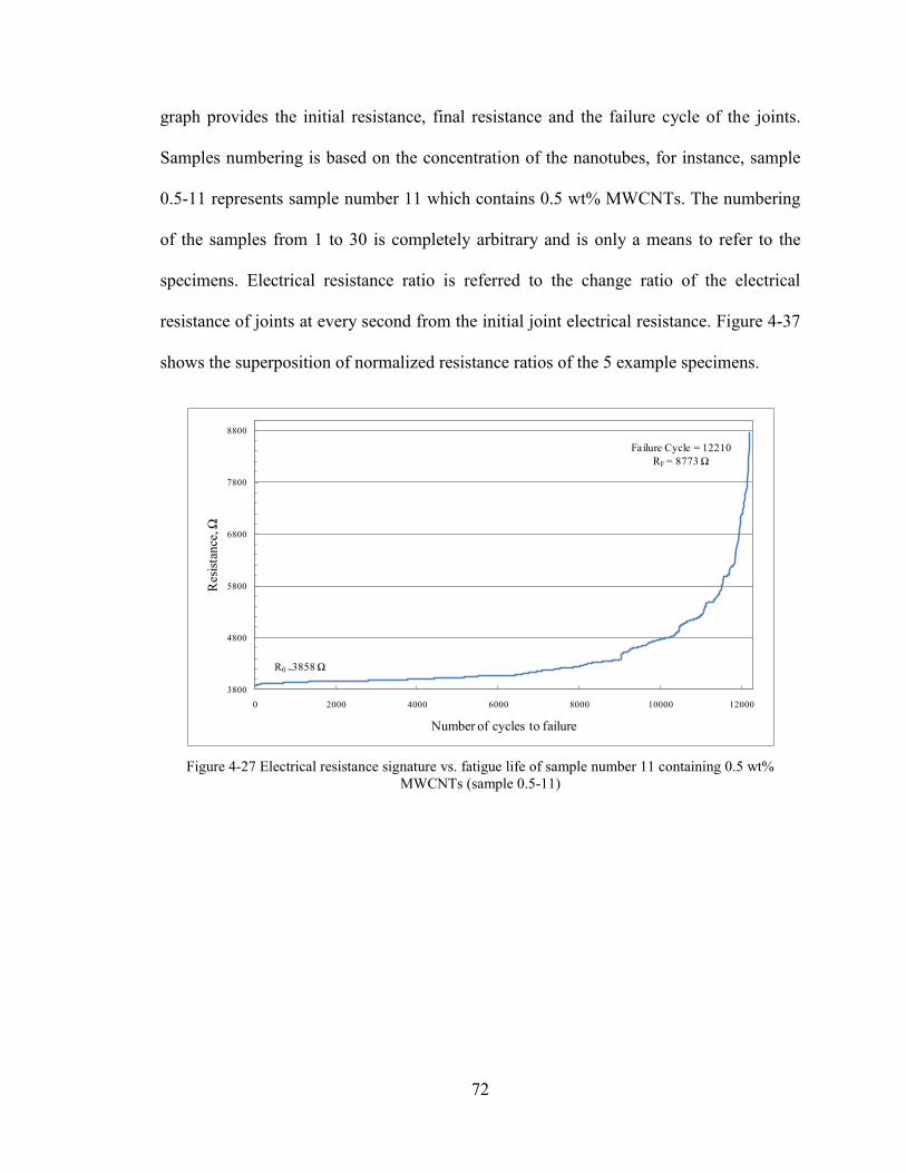
72
graph provides the initial resistance, final resistance and the failure cycle of the joints.
Samples numbering is based on the concentration of the nanotubes, for instance, sample
0.5-11 represents sample number 11 which contains 0.5 wt% MWCNTs. The numbering
of the samples from 1 to 30 is completely arbitrary and is only a means to refer to the
specimens. Electrical resistance ratio is referred to the change ratio of the electrical
resistance of joints at every second from the initial joint electrical resistance. Figure 4-37
shows the superposition of normalized resistance ratios of the 5 example specimens.
Figure 4-27 Electrical resistance signature vs. fatigue life of sample number 11 containing 0.5 wt%
MWCNTs (sample 0.5-11)
R0 =3858 Ω
Failure Cycle = 12210
RF = 8773 Ω
3800
4800
5800
6800
7800
8800
0 2000 4000 6000 8000 10000 12000
Res
ista
nce
, Ω
Number of cycles to failure

73
Figure 4-28 Electrical resistance ratio vs. fatigue life for sample 0.5-11
Figure 4-29 Electrical resistance signature vs. fatigue life of sample number 15 containing 0.5 wt%
MWCNTs (sample 0.5-15)
0
0.2
0.4
0.6
0.8
1
1.2
1.4
0 0.1 0.2 0.3 0.4 0.5 0.6 0.7 0.8 0.9 1
∆R
/Ro
Number of cycles to faiulre / Final failure
R0 = 6483 Ω
Failure Cycle = 9310RF = 9173 Ω
6483
6983
7483
7983
8483
8983
9483
0 1000 2000 3000 4000 5000 6000 7000 8000 9000
Res
ista
nce
, Ω
Number of cycles to failure
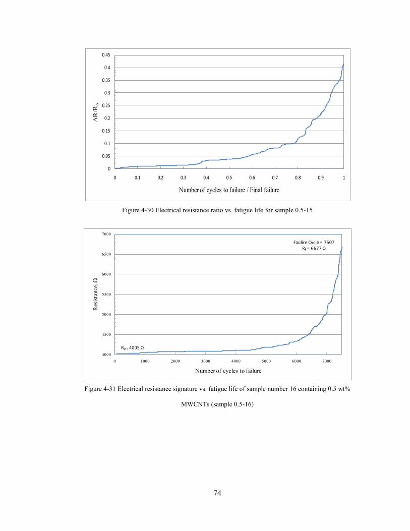
74
Figure 4-30 Electrical resistance ratio vs. fatigue life for sample 0.5-15
Figure 4-31 Electrical resistance signature vs. fatigue life of sample number 16 containing 0.5 wt%
MWCNTs (sample 0.5-16)
0
0.05
0.1
0.15
0.2
0.25
0.3
0.35
0.4
0.45
0 0.1 0.2 0.3 0.4 0.5 0.6 0.7 0.8 0.9 1
∆R
/Ro
Number of cycles to failure / Final failure
R0 = 4005 Ω
Faulire Cycle = 7507RF = 6677 Ω
4000
4500
5000
5500
6000
6500
7000
0 1000 2000 3000 4000 5000 6000 7000
Res
ista
nce
, Ω
Number of cycles to failure
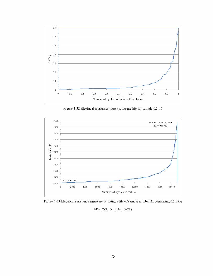
75
Figure 4-32 Electrical resistance ratio vs. fatigue life for sample 0.5-16
Figure 4-33 Electrical resistance signature vs. fatigue life of sample number 21 containing 0.5 wt%
MWCNTs (sample 0.5-21)
0
0.1
0.2
0.3
0.4
0.5
0.6
0.7
0 0.1 0.2 0.3 0.4 0.5 0.6 0.7 0.8 0.9 1
∆R
/Ro
Number of cycles to failure / Final failure
R0 = 4917 Ω
Failure Cycle =18840
RF = 9607 Ω
4900
5400
5900
6400
6900
7400
7900
8400
8900
9400
9900
0 2000 4000 6000 8000 10000 12000 14000 16000 18000
Res
ista
nce
, Ω
Number of cycles to failure
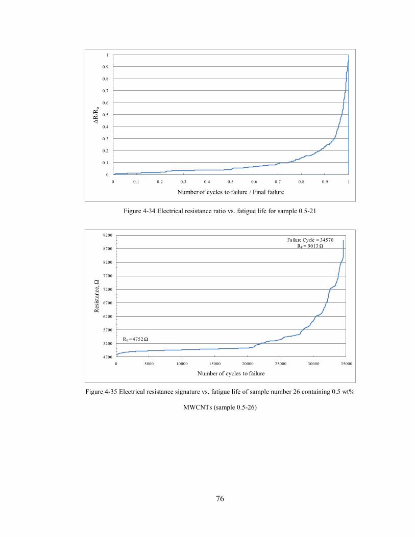
76
Figure 4-34 Electrical resistance ratio vs. fatigue life for sample 0.5-21
Figure 4-35 Electrical resistance signature vs. fatigue life of sample number 26 containing 0.5 wt%
MWCNTs (sample 0.5-26)
0
0.1
0.2
0.3
0.4
0.5
0.6
0.7
0.8
0.9
1
0 0.1 0.2 0.3 0.4 0.5 0.6 0.7 0.8 0.9 1
∆R
/Ro
Number of cycles to failure / Final failure
R0 = 4752 Ω
Failure Cycle = 34570
RF = 9013 Ω
4700
5200
5700
6200
6700
7200
7700
8200
8700
9200
0 5000 10000 15000 20000 25000 30000 35000
Res
ista
nce
, Ω
Number of cycles to failure
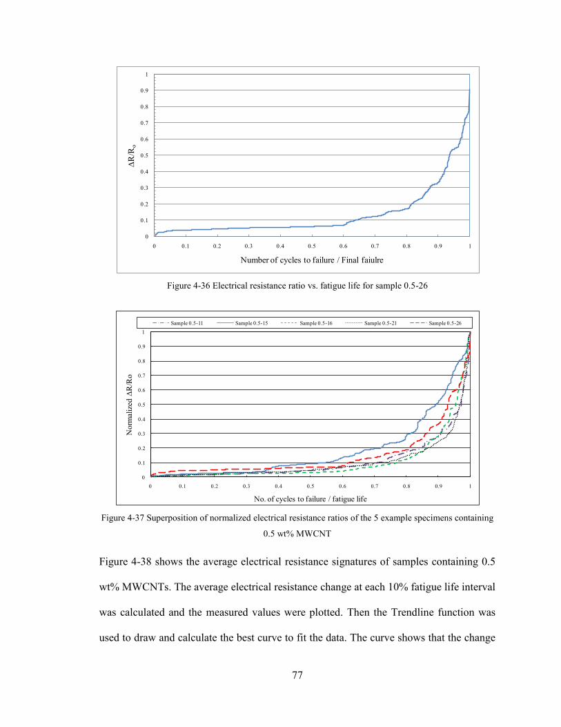
77
Figure 4-36 Electrical resistance ratio vs. fatigue life for sample 0.5-26
Figure 4-37 Superposition of normalized electrical resistance ratios of the 5 example specimens containing
0.5 wt% MWCNT
Figure 4-38 shows the average electrical resistance signatures of samples containing 0.5
wt% MWCNTs. The average electrical resistance change at each 10% fatigue life interval
was calculated and the measured values were plotted. Then the Trendline function was
used to draw and calculate the best curve to fit the data. The curve shows that the change
0
0.1
0.2
0.3
0.4
0.5
0.6
0.7
0.8
0.9
1
0 0.1 0.2 0.3 0.4 0.5 0.6 0.7 0.8 0.9 1
∆R
/Ro
Number of cycles to failure / Final faiulre
0
0.1
0.2
0.3
0.4
0.5
0.6
0.7
0.8
0.9
1
0 0.1 0.2 0.3 0.4 0.5 0.6 0.7 0.8 0.9 1
No
rmal
ized
∆R
/Ro
No. of cycles to failure / fatigue life
Sample 0.5-11 Sample 0.5-15 Sample 0.5-16 Sample 0.5-21 Sample 0.5-26
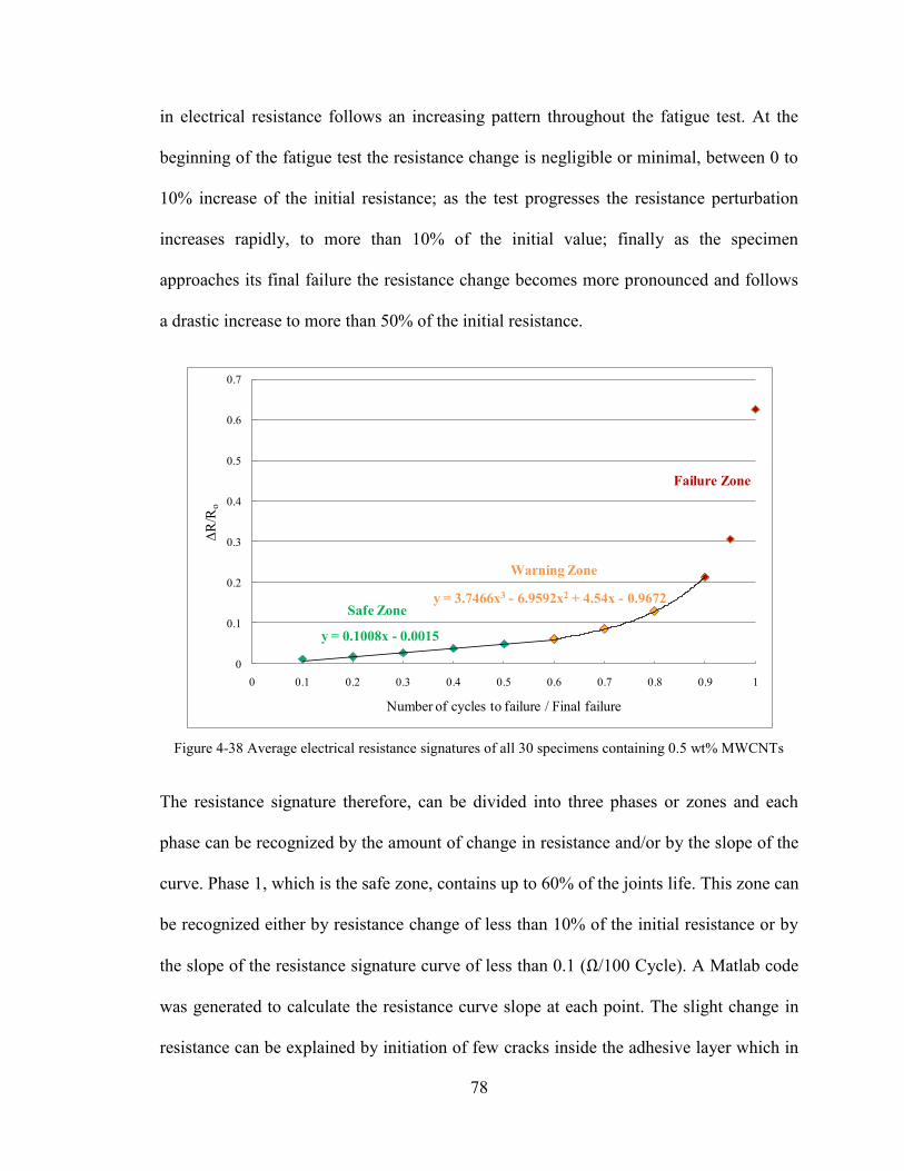
78
in electrical resistance follows an increasing pattern throughout the fatigue test. At the
beginning of the fatigue test the resistance change is negligible or minimal, between 0 to
10% increase of the initial resistance; as the test progresses the resistance perturbation
increases rapidly, to more than 10% of the initial value; finally as the specimen
approaches its final failure the resistance change becomes more pronounced and follows
a drastic increase to more than 50% of the initial resistance.
Figure 4-38 Average electrical resistance signatures of all 30 specimens containing 0.5 wt% MWCNTs
The resistance signature therefore, can be divided into three phases or zones and each
phase can be recognized by the amount of change in resistance and/or by the slope of the
curve. Phase 1, which is the safe zone, contains up to 60% of the joints life. This zone can
be recognized either by resistance change of less than 10% of the initial resistance or by
the slope of the resistance signature curve of less than 0.1 (Ω/100 Cycle). A Matlab code
was generated to calculate the resistance curve slope at each point. The slight change in
resistance can be explained by initiation of few cracks inside the adhesive layer which in
y = 0.1008x - 0.0015
y = 3.7466x3 - 6.9592x2 + 4.54x - 0.9672
0
0.1
0.2
0.3
0.4
0.5
0.6
0.7
0 0.1 0.2 0.3 0.4 0.5 0.6 0.7 0.8 0.9 1
∆R
/Ro
Number of cycles to failure / Final failure
Failure Zone
Warning Zone
Safe Zone
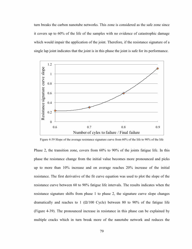
79
turn breaks the carbon nanotube networks. This zone is considered as the safe zone since
it covers up to 60% of the life of the samples with no evidence of catastrophic damage
which would impair the application of the joint. Therefore, if the resistance signature of a
single lap joint indicates that the joint is in this phase the joint is safe for its performance.
Figure 4-39 Slope of the average resistance signature curve from 60% of the life to 90% of the life
Phase 2, the transition zone, covers from 60% to 90% of the joints fatigue life. In this
phase the resistance change from the initial value becomes more pronounced and picks
up to more than 10% increase and on average reaches 20% increase of the initial
resistance. The first derivative of the fit curve equation was used to plot the slope of the
resistance curve between 60 to 90% fatigue life intervals. The results indicates when the
resistance signature shifts from phase 1 to phase 2, the signature curve slope changes
dramatically and reaches to 1 (Ω/100 Cycle) between 80 to 90% of the fatigue life
(Figure 4-39). The pronounced increase in resistance in this phase can be explained by
multiple cracks which in turn break more of the nanotube network and reduces the
0
0.2
0.4
0.6
0.8
1
1.2
0.6 0.7 0.8 0.9
Res
ista
nce
sig
nat
ure
curv
e sl
ope
Number of cyles to failure / Final failure

80
number of electrical paths dramatically. Figure 4-40 shows SEM images of multiple
cracks in the form of striation on the fracture surface of the adhesive joints which
contributed to the dramatic increase in the resistance. This zone is considered as the
caution zone or warning zone. Two warning points are associated with this zone, the first
is the resistance change of more than 10%+2% of the initial value which for 93% of the
samples occurred between 60 to 90% of the fatigue life, and the second warning point is
the change in the signature curve slope of more than 1 (Ω/100 Cycle) which in 93% of the
samples corresponded to 80%-3%to 90%+3% of their fatigue life. Therefore, if the
resistance signature indicates that the joint is in this phase, more caution should be
applied and depending upon the joint application proper measures, such as repair,
strengthening or complete replacement should be executed to ensure the safe
performance of the joint. Phase 3, the final or failure phase, contains the last 10% of the
fatigue life of the joint. In this phase the electrical resistance changes dramatically up to
100% of the initial resistance or even more. The slope of the curve is changing rapidly
and on average reaches more than 4 (Ω/100 Cycle) to almost 80 (Ω/100 Cycle) which
indicates a nonlinear curve with sharp increase in its slope. In this phase, multiple crack
and delamination between the adhesive layer and substrates are responsible for the
nonlinear dramatic increase in resistance. The delamination between the adhesive layer
and the substrate can be recorded using long-distance microscope; delamination may also
occur around the end of phase 2. Figure 4-41 shows the long distance microscopic image
of sample 0.5-7. The images show the edge of the sample at a) the beginning of the test,
at b) before 60% of the fatigue life while resistance change was less than 10% of the
initial value at c) 91% of the life while the first sign of delamination was seen and the
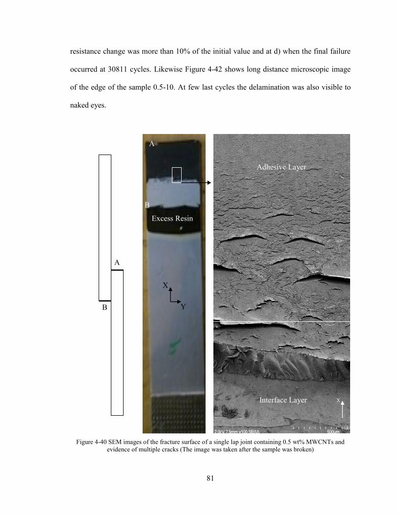
81
resistance change was more than 10% of the initial value and at d) when the final failure
occurred at 30811 cycles. Likewise Figure 4-42 shows long distance microscopic image
of the edge of the sample 0.5-10. At few last cycles the delamination was also visible to
naked eyes.
Figure 4-40 SEM images of the fracture surface of a single lap joint containing 0.5 wt% MWCNTs and
evidence of multiple cracks (The image was taken after the sample was broken)
X
Y
X
Excess Resin
A
B
A
B
Adhesive Layer
Interface Layer
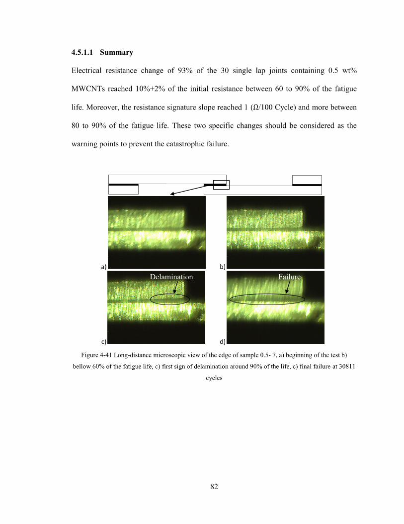
82
4.5.1.1 Summary
Electrical resistance change of 93% of the 30 single lap joints containing 0.5 wt%
MWCNTs reached 10%+2% of the initial resistance between 60 to 90% of the fatigue
life. Moreover, the resistance signature slope reached 1 (Ω/100 Cycle) and more between
80 to 90% of the fatigue life. These two specific changes should be considered as the
warning points to prevent the catastrophic failure.
Figure 4-41 Long-distance microscopic view of the edge of sample 0.5- 7, a) beginning of the test b)
bellow 60% of the fatigue life, c) first sign of delamination around 90% of the life, c) final failure at 30811
cycles
4 in
¾ in 1 in
adhesive thickness
= 0.078 inch
a) b)
c) d)
Delamination Failure
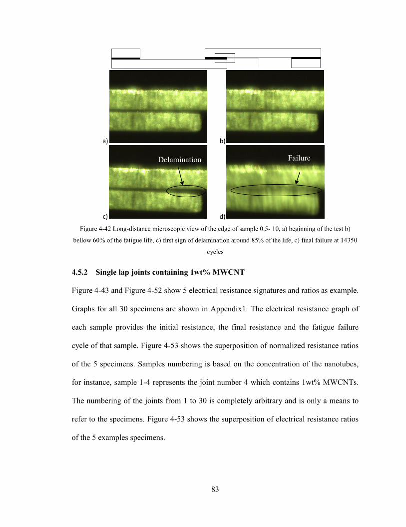
83
Figure 4-42 Long-distance microscopic view of the edge of sample 0.5- 10, a) beginning of the test b)
bellow 60% of the fatigue life, c) first sign of delamination around 85% of the life, c) final failure at 14350
cycles
4.5.2 Single lap joints containing 1wt% MWCNT
Figure 4-43 and Figure 4-52 show 5 electrical resistance signatures and ratios as example.
Graphs for all 30 specimens are shown in Appendix1. The electrical resistance graph of
each sample provides the initial resistance, the final resistance and the fatigue failure
cycle of that sample. Figure 4-53 shows the superposition of normalized resistance ratios
of the 5 specimens. Samples numbering is based on the concentration of the nanotubes,
for instance, sample 1-4 represents the joint number 4 which contains 1wt% MWCNTs.
The numbering of the joints from 1 to 30 is completely arbitrary and is only a means to
refer to the specimens. Figure 4-53 shows the superposition of electrical resistance ratios
of the 5 examples specimens.
4 in
¾ in1 in
adhesive thickness
= 0.078 inch
a) b)
c) d)
Delamination Failure

84
Figure 4-43 Electrical resistance signature vs. fatigue life of sample number 4 containing 1 wt% MWCNTs
(sample 1-4)
Figure 4-44 Electrical resistance ratio vs. fatigue life for sample 1-4
1800
2300
2800
3300
3800
4300
0 1000 2000 3000 4000 5000
Resi
stance, Ω
Number of cycles to failure
Ro = 1880 Ω
Failure Cycle = 5785
RF = 4059 Ω
0
0.2
0.4
0.6
0.8
1
1.2
0 0.1 0.2 0.3 0.4 0.5 0.6 0.7 0.8 0.9 1
∆R
/Ro
Number of cycles to failure / Final failure
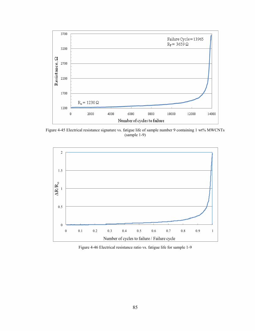
85
Figure 4-45 Electrical resistance signature vs. fatigue life of sample number 9 containing 1 wt% MWCNTs
(sample 1-9)
Figure 4-46 Electrical resistance ratio vs. fatigue life for sample 1-9
0
0.5
1
1.5
2
0 0.1 0.2 0.3 0.4 0.5 0.6 0.7 0.8 0.9 1
∆R
/Ro
Number of cycles to failure / Failure cycle
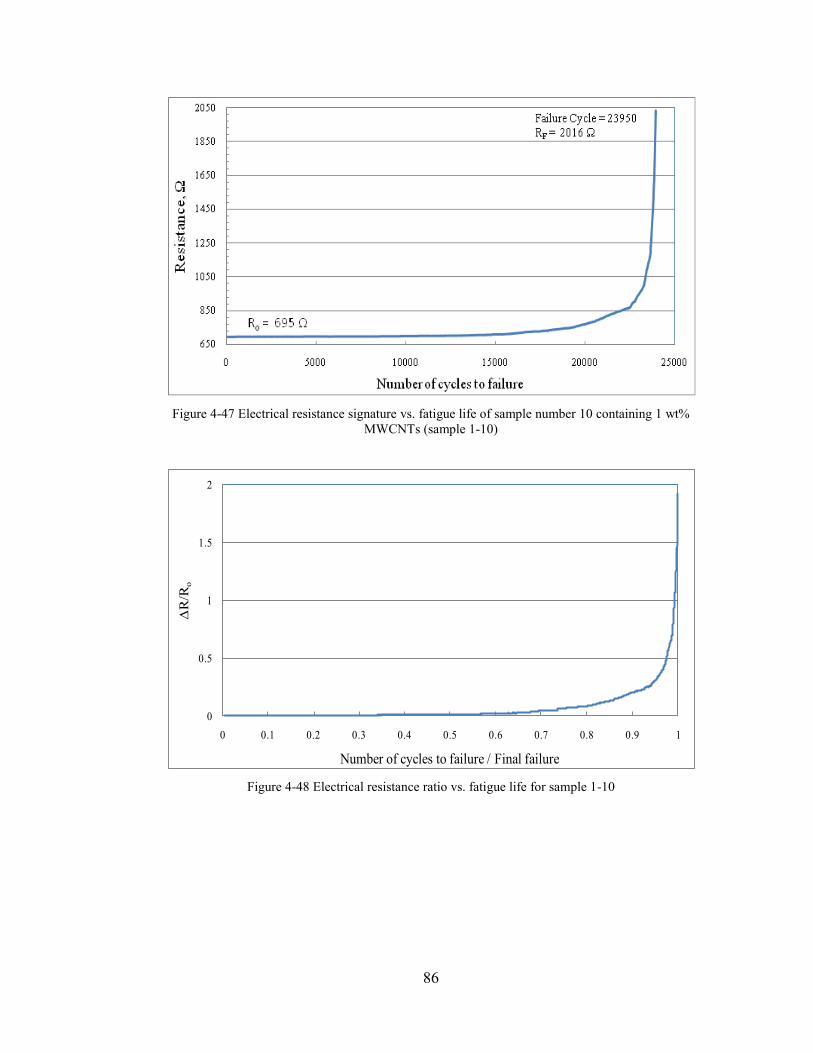
86
Figure 4-47 Electrical resistance signature vs. fatigue life of sample number 10 containing 1 wt%
MWCNTs (sample 1-10)
Figure 4-48 Electrical resistance ratio vs. fatigue life for sample 1-10
0
0.5
1
1.5
2
0 0.1 0.2 0.3 0.4 0.5 0.6 0.7 0.8 0.9 1
∆R
/Ro
Number of cycles to failure / Final failure
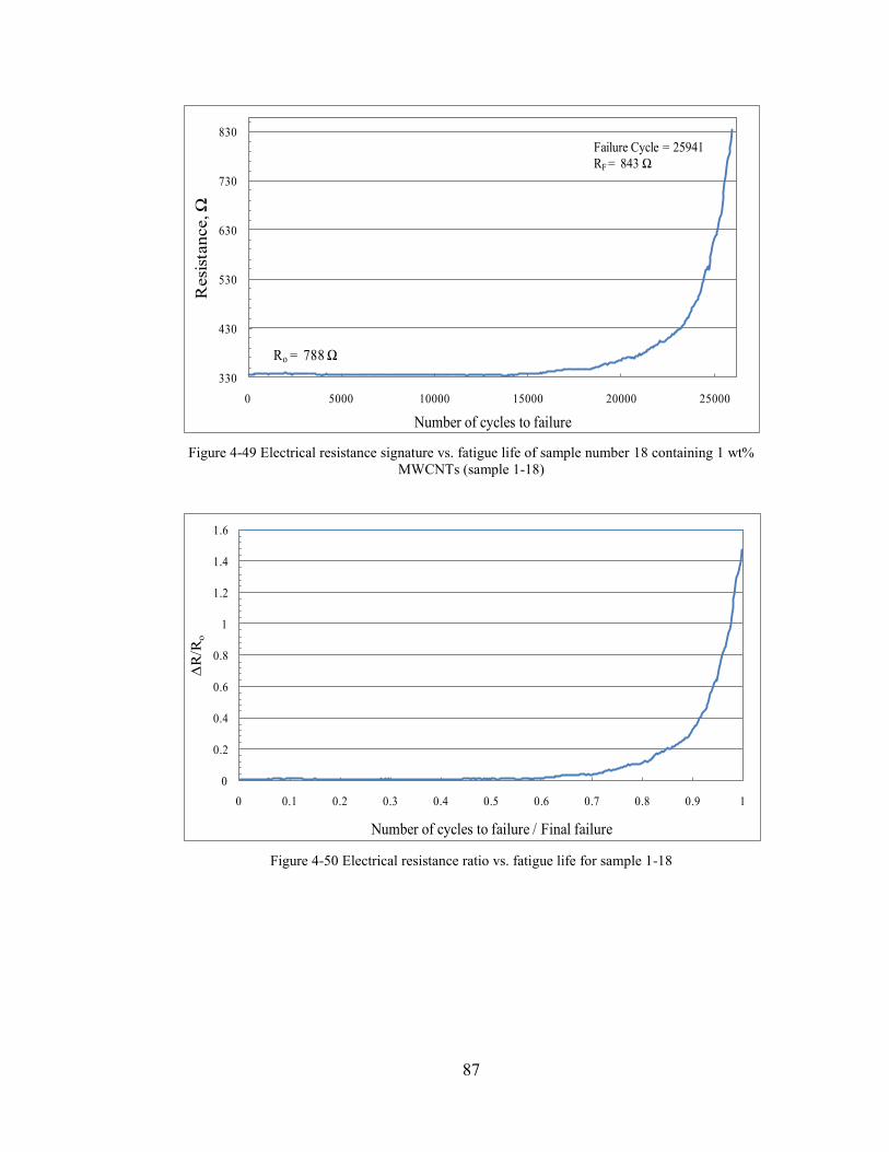
87
Figure 4-49 Electrical resistance signature vs. fatigue life of sample number 18 containing 1 wt%
MWCNTs (sample 1-18)
Figure 4-50 Electrical resistance ratio vs. fatigue life for sample 1-18
330
430
530
630
730
830
0 5000 10000 15000 20000 25000
Resi
stan
ce, Ω
Number of cycles to failure
Ro = 788 Ω
Failure Cycle = 25941
RF = 843 Ω
0
0.2
0.4
0.6
0.8
1
1.2
1.4
1.6
0 0.1 0.2 0.3 0.4 0.5 0.6 0.7 0.8 0.9 1
∆R
/Ro
Number of cycles to failure / Final failure
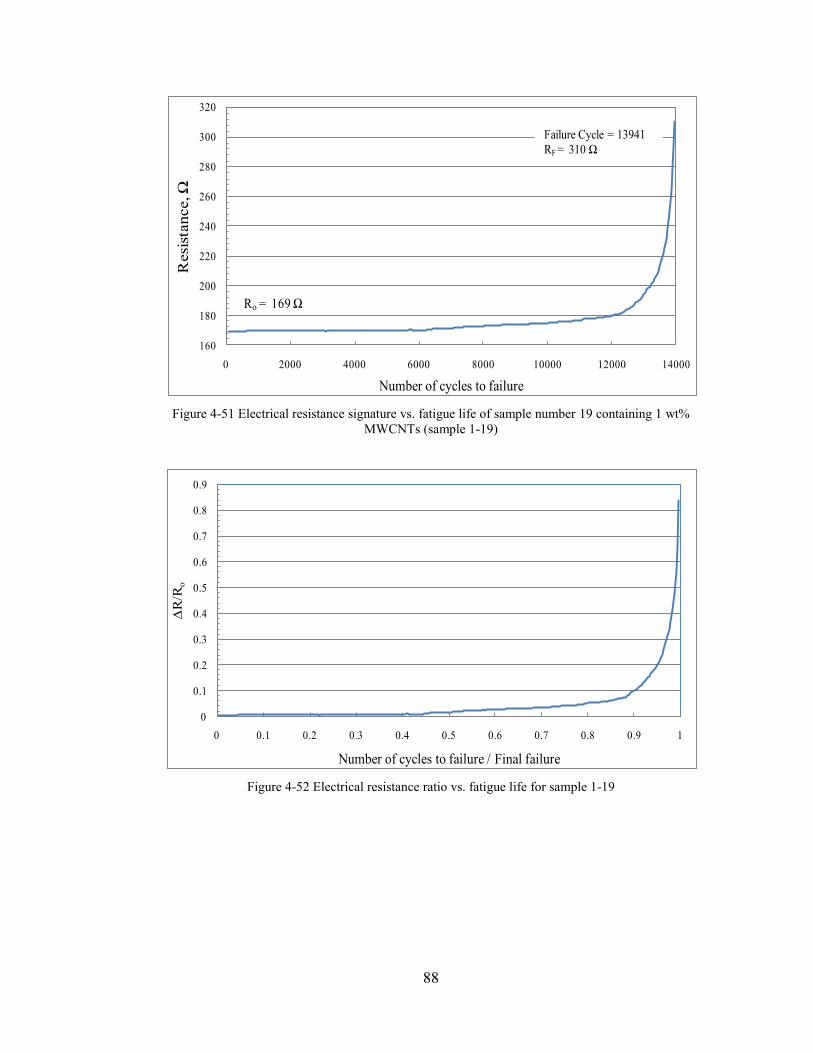
88
Figure 4-51 Electrical resistance signature vs. fatigue life of sample number 19 containing 1 wt%
MWCNTs (sample 1-19)
Figure 4-52 Electrical resistance ratio vs. fatigue life for sample 1-19
160
180
200
220
240
260
280
300
320
0 2000 4000 6000 8000 10000 12000 14000
Resi
stan
ce, Ω
Number of cycles to failure
Ro = 169 Ω
Failure Cycle = 13941
RF = 310 Ω
0
0.1
0.2
0.3
0.4
0.5
0.6
0.7
0.8
0.9
0 0.1 0.2 0.3 0.4 0.5 0.6 0.7 0.8 0.9 1
∆R
/Ro
Number of cycles to failure / Final failure

89
Figure 4-53 Superposition of normalized electrical resistance ratios of the 5 example specimens containing
1wt% MWCNT
Figure 4-54 The average electrical resistance signatures of all 30 specimens containing 1wt% MWCNTs
The average electrical resistance change at each 10% fatigue life interval was calculated
and the measured values were plotted. Then the Trendline function was used to draw and
calculate the best curve to fit the data. The average electrical resistance signatures of the
0
0.1
0.2
0.3
0.4
0.5
0.6
0.7
0.8
0.9
1
0 0.1 0.2 0.3 0.4 0.5 0.6 0.7 0.8 0.9 1
∆R
/Ro
No. of cycles to failure / fatigue life
Sample 1-4 Sample 1-9 Sample 1-10 Sample 1-18 Sample 1-19
y = 0.0672x - 0.0041
y = 12.028x3 - 23.837x2 + 15.965x - 3.5559
0
0.1
0.2
0.3
0.4
0.5
0.6
0.7
0.8
0.9
1
1.1
1.2
1.3
1.4
0 0.1 0.2 0.3 0.4 0.5 0.6 0.7 0.8 0.9 1 1.1
∆R
/Ro
Number of cycles to failure / Final failure
Safe Zone
Warning Zone
Failure Zone
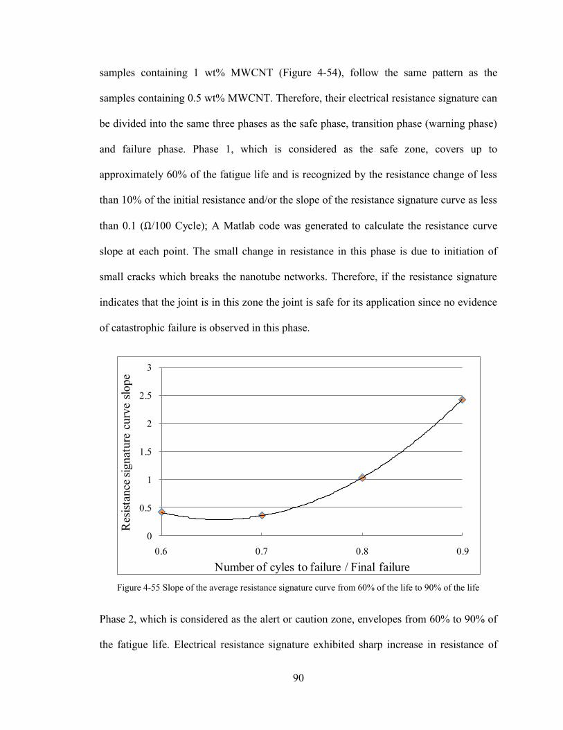
90
samples containing 1 wt% MWCNT (Figure 4-54), follow the same pattern as the
samples containing 0.5 wt% MWCNT. Therefore, their electrical resistance signature can
be divided into the same three phases as the safe phase, transition phase (warning phase)
and failure phase. Phase 1, which is considered as the safe zone, covers up to
approximately 60% of the fatigue life and is recognized by the resistance change of less
than 10% of the initial resistance and/or the slope of the resistance signature curve as less
than 0.1 (Ω/100 Cycle); A Matlab code was generated to calculate the resistance curve
slope at each point. The small change in resistance in this phase is due to initiation of
small cracks which breaks the nanotube networks. Therefore, if the resistance signature
indicates that the joint is in this zone the joint is safe for its application since no evidence
of catastrophic failure is observed in this phase.
Figure 4-55 Slope of the average resistance signature curve from 60% of the life to 90% of the life
Phase 2, which is considered as the alert or caution zone, envelopes from 60% to 90% of
the fatigue life. Electrical resistance signature exhibited sharp increase in resistance of
0
0.5
1
1.5
2
2.5
3
0.6 0.7 0.8 0.9
Res
ista
nce
sig
nat
ure
curv
e sl
ope
Number of cyles to failure / Final failure
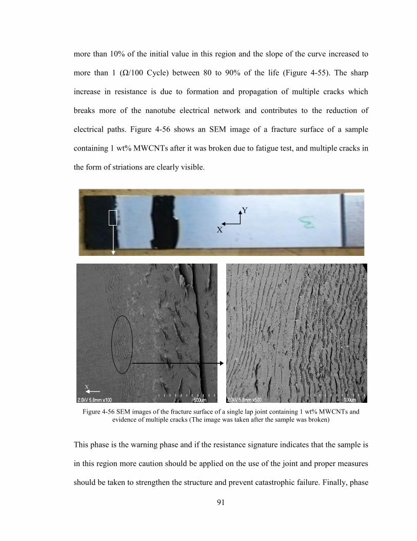
91
more than 10% of the initial value in this region and the slope of the curve increased to
more than 1 (Ω/100 Cycle) between 80 to 90% of the life (Figure 4-55). The sharp
increase in resistance is due to formation and propagation of multiple cracks which
breaks more of the nanotube electrical network and contributes to the reduction of
electrical paths. Figure 4-56 shows an SEM image of a fracture surface of a sample
containing 1 wt% MWCNTs after it was broken due to fatigue test, and multiple cracks in
the form of striations are clearly visible.
Figure 4-56 SEM images of the fracture surface of a single lap joint containing 1 wt% MWCNTs and
evidence of multiple cracks (The image was taken after the sample was broken)
This phase is the warning phase and if the resistance signature indicates that the sample is
in this region more caution should be applied on the use of the joint and proper measures
should be taken to strengthen the structure and prevent catastrophic failure. Finally, phase
Y
X
X
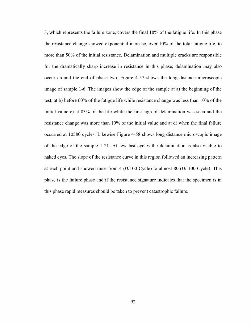
92
3, which represents the failure zone, covers the final 10% of the fatigue life. In this phase
the resistance change showed exponential increase, over 10% of the total fatigue life, to
more than 50% of the initial resistance. Delamination and multiple cracks are responsible
for the dramatically sharp increase in resistance in this phase; delamination may also
occur around the end of phase two. Figure 4-57 shows the long distance microscopic
image of sample 1-6. The images show the edge of the sample at a) the beginning of the
test, at b) before 60% of the fatigue life while resistance change was less than 10% of the
initial value c) at 83% of the life while the first sign of delamination was seen and the
resistance change was more than 10% of the initial value and at d) when the final failure
occurred at 10580 cycles. Likewise Figure 4-58 shows long distance microscopic image
of the edge of the sample 1-21. At few last cycles the delamination is also visible to
naked eyes. The slope of the resistance curve in this region followed an increasing pattern
at each point and showed raise from 4 (Ω/100 Cycle) to almost 80 (Ω/ 100 Cycle). This
phase is the failure phase and if the resistance signature indicates that the specimen is in
this phase rapid measures should be taken to prevent catastrophic failure.

93
Figure 4-57 Long-distance microscopic view of the edge of sample 1- 6, a) beginning of the test b) bellow
60% of the fatigue life, c) first sign of delamination around 83% of the life, d) final failure at 10580 cycles
Figure 4-58 Long-distance microscopic view of the edge of sample 1- 21, a) beginning of the test b) bellow
60% of the fatigue life, c) first sign of delamination around 88% of the life, d) final failure at 7041cycles
4 in
¾ in 1 in
adhesive thickness
= 0.078 inch
a) b)
c) d)
a) b)
d) e)
a) b)
d) e)
a) b)
d) e)
a) b)
d) e)
4 in
¾ in1 in
adhesive thickness
= 0.078 inch
a) b)
c) d)
Failure Delamination
Delamination Failure

94
4.5.2.1 Summary
The results of 90% of the 30 specimens containing 1 wt% MWCNTs showed increase of
more than 10%+2% of the initial resistance between 60% to 90% of their fatigue life. The
specific increase of 10% in resistance should be taken as the first warning point and more
caution should be taken in the application of the joints. Moreover, in 97% of the
specimens the change in the resistance curve slope to more than 1 (Ω/100 Cycle) occurred
between 80%-4% to 90%+4%of their fatigue lives. The slope change of more than 1 (Ω/
100 Cycle) should be considered as the second warning and necessary measures should
be taken to strengthen, repair and/or replacing the joint according to the end user
requirements.
4.5.3 Single lap joints containing 2 wt% MWCNT
Figure 4-59 and Figure 4-68 show the electrical resistance signatures and ratios of all 5
specimens containing 2 wt% MWCNT. The electrical resistance graph of each sample
provides the initial resistance, the final resistance and the fatigue failure cycle of that
sample. Samples numbering is based on the concentration of the nanotubes, for instance,
sample 2-1 represents the joint number 1 which contains 2 wt% MWCNTs. The
numbering of the joints from 1 to 5 is completely arbitrary and is only a mean to refer to
the specimens. Figure 4-69 shows the superposition of the electrical resistance ratios.

95
Figure 4-59 Electrical resistance signature vs. fatigue life of sample number 1 containing 2 wt% MWCNTs
(sample 2-1)
Figure 4-60 Electrical resistance ratio vs. fatigue life for sample 2-1
0
0.2
0.4
0.6
0.8
1
1.2
0 0.1 0.2 0.3 0.4 0.5 0.6 0.7 0.8 0.9 1
∆R
/Ro
Number of cycles to failure / Final failure

96
Figure 4-61 Electrical resistance signature vs. fatigue life of sample number 2 containing 2 wt% MWCNTs
(sample 2-2)
Figure 4-62 Electrical resistance ratio vs. fatigue life for sample 2-2
43
45
47
49
51
53
55
57
0 500 1000 1500 2000 2500 3000 3500
Resi
stan
ce, Ω
Number of cycles to failure
Ro = 43 Ω
Failure Cycle = 3637
RF = 57 Ω
0
0.05
0.1
0.15
0.2
0.25
0.3
0.35
0 0.1 0.2 0.3 0.4 0.5 0.6 0.7 0.8 0.9 1
∆R
/Ro
Number of cycles to failure / Final failure

97
Figure 4-63 Electrical resistance signature vs. fatigue life of sample number 3 containing 2 wt% MWCNTs
(sample 2-3)
Figure 4-64 Electrical resistance ratio vs. fatigue life for sample 2-3
0
0.2
0.4
0.6
0.8
1
1.2
1.4
0 0.1 0.2 0.3 0.4 0.5 0.6 0.7 0.8 0.9 1
∆R
/Ro
Number of cycles to failure / Final failure

98
Figure 4-65 Electrical resistance signature vs. fatigue life of sample number 4 containing 2 wt% MWCNTs
(sample 2-4)
Figure 4-66 Electrical resistance ratio vs. fatigue life for sample 2-4
54
64
74
84
94
104
114
0 500 1000 1500 2000 2500 3000
Resi
stan
ce, Ω
Number of cycles to failure
Ro = 54 Ω
Failure Cycle = 2914
RF = 108 Ω
0
0.1
0.2
0.3
0.4
0.5
0.6
0.7
0.8
0.9
1
0 0.1 0.2 0.3 0.4 0.5 0.6 0.7 0.8 0.9 1
∆R
/Ro
Number of cycles to failure / Final failure
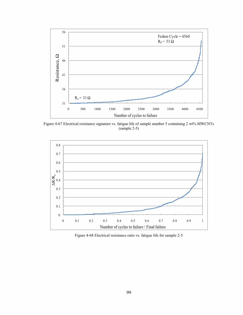
99
Figure 4-67 Electrical resistance signature vs. fatigue life of sample number 5 containing 2 wt% MWCNTs
(sample 2-5)
Figure 4-68 Electrical resistance ratio vs. fatigue life for sample 2-5
31
36
41
46
51
56
0 500 1000 1500 2000 2500 3000 3500 4000 4500
Resi
stan
ce, Ω
Number of cycles to failure
Ro = 31 Ω
Failure Cycle = 4560
RF = 53 Ω
0
0.1
0.2
0.3
0.4
0.5
0.6
0.7
0.8
0 0.1 0.2 0.3 0.4 0.5 0.6 0.7 0.8 0.9 1
∆R
/Ro
Number of cycles to failure / Final failure
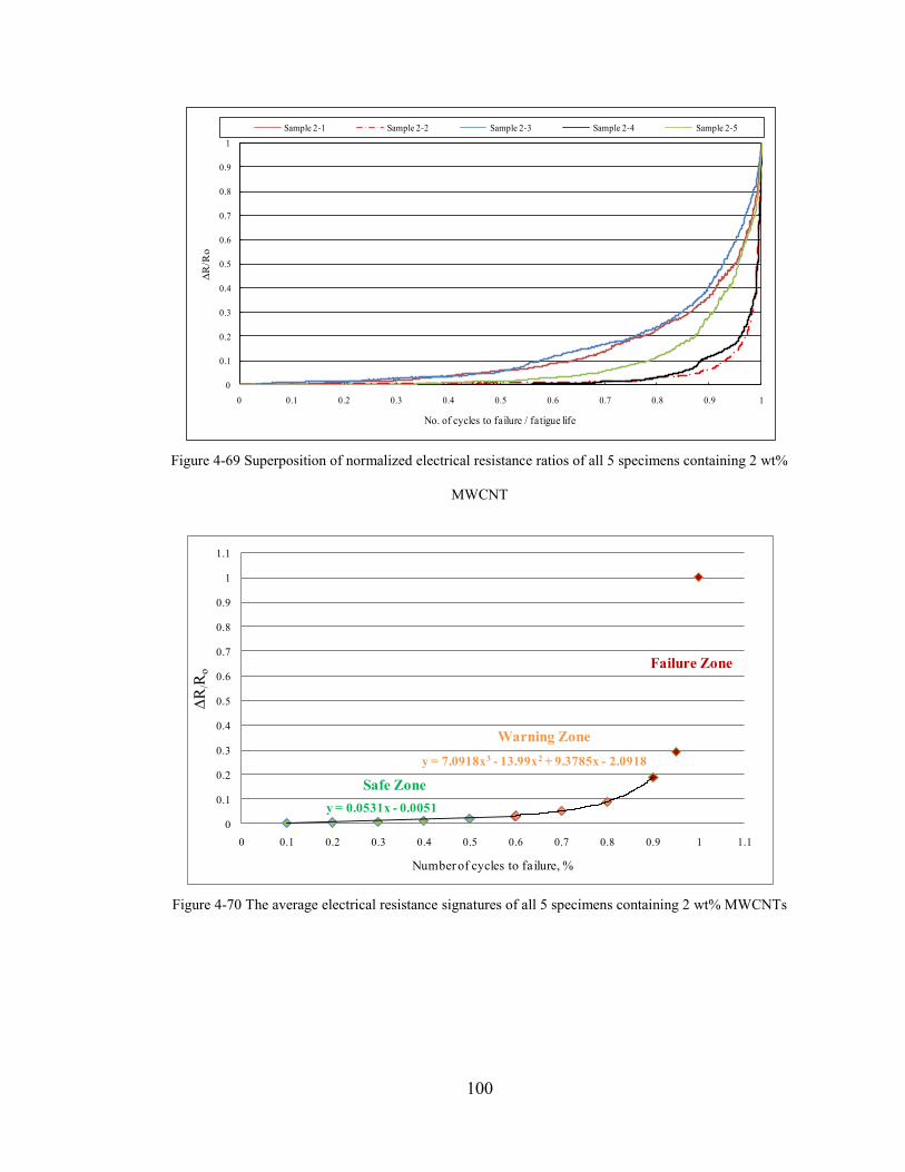
100
Figure 4-69 Superposition of normalized electrical resistance ratios of all 5 specimens containing 2 wt%
MWCNT
Figure 4-70 The average electrical resistance signatures of all 5 specimens containing 2 wt% MWCNTs
0
0.1
0.2
0.3
0.4
0.5
0.6
0.7
0.8
0.9
1
0 0.1 0.2 0.3 0.4 0.5 0.6 0.7 0.8 0.9 1
∆R
/Ro
No. of cycles to failure / fatigue life
Sample 2-1 Sample 2-2 Sample 2-3 Sample 2-4 Sample 2-5
Phase 1 : Safe Zone
Phase 3 : Failure Zone
Phase 2 : Transition Region
y = 0.0531x - 0.0051
y = 7.0918x3 - 13.99x2 + 9.3785x - 2.0918
0
0.1
0.2
0.3
0.4
0.5
0.6
0.7
0.8
0.9
1
1.1
0 0.1 0.2 0.3 0.4 0.5 0.6 0.7 0.8 0.9 1 1.1
∆R
/Ro
Number of cycles to failure, %
Safe Zone
Warning Zone
Failure Zone
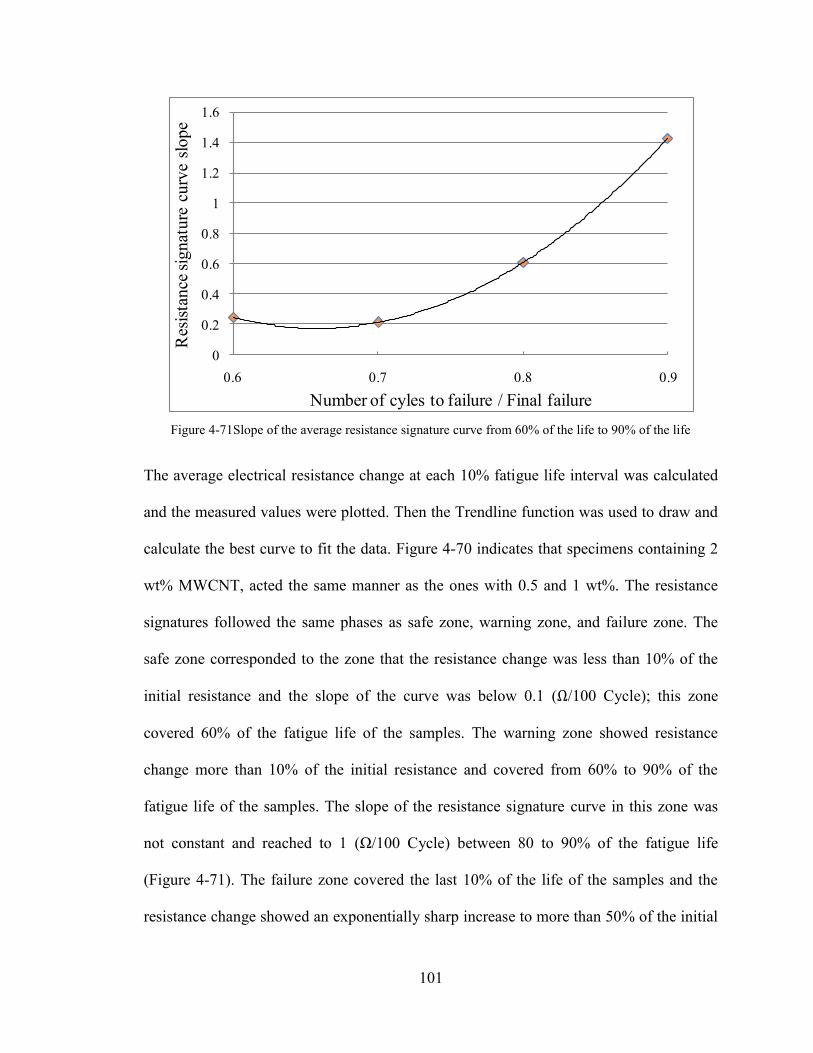
101
Figure 4-71Slope of the average resistance signature curve from 60% of the life to 90% of the life
The average electrical resistance change at each 10% fatigue life interval was calculated
and the measured values were plotted. Then the Trendline function was used to draw and
calculate the best curve to fit the data. Figure 4-70 indicates that specimens containing 2
wt% MWCNT, acted the same manner as the ones with 0.5 and 1 wt%. The resistance
signatures followed the same phases as safe zone, warning zone, and failure zone. The
safe zone corresponded to the zone that the resistance change was less than 10% of the
initial resistance and the slope of the curve was below 0.1 (Ω/100 Cycle); this zone
covered 60% of the fatigue life of the samples. The warning zone showed resistance
change more than 10% of the initial resistance and covered from 60% to 90% of the
fatigue life of the samples. The slope of the resistance signature curve in this zone was
not constant and reached to 1 (Ω/100 Cycle) between 80 to 90% of the fatigue life
(Figure 4-71). The failure zone covered the last 10% of the life of the samples and the
resistance change showed an exponentially sharp increase to more than 50% of the initial
0
0.2
0.4
0.6
0.8
1
1.2
1.4
1.6
0.6 0.7 0.8 0.9
Res
ista
nce
sig
nat
ure
curv
e sl
ope
Number of cyles to failure / Final failure
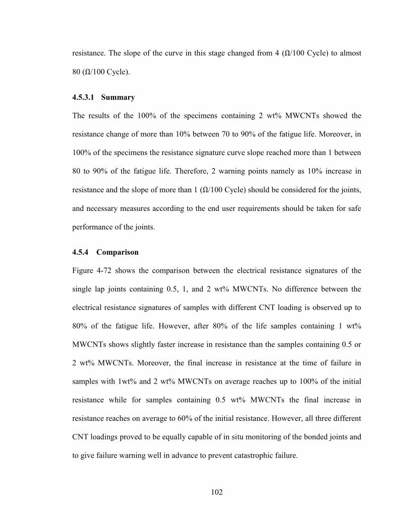
102
resistance. The slope of the curve in this stage changed from 4 (Ω/100 Cycle) to almost
80 (Ω/100 Cycle).
4.5.3.1 Summary
The results of the 100% of the specimens containing 2 wt% MWCNTs showed the
resistance change of more than 10% between 70 to 90% of the fatigue life. Moreover, in
100% of the specimens the resistance signature curve slope reached more than 1 between
80 to 90% of the fatigue life. Therefore, 2 warning points namely as 10% increase in
resistance and the slope of more than 1 (Ω/100 Cycle) should be considered for the joints,
and necessary measures according to the end user requirements should be taken for safe
performance of the joints.
4.5.4 Comparison
Figure 4-72 shows the comparison between the electrical resistance signatures of the
single lap joints containing 0.5, 1, and 2 wt% MWCNTs. No difference between the
electrical resistance signatures of samples with different CNT loading is observed up to
80% of the fatigue life. However, after 80% of the life samples containing 1 wt%
MWCNTs shows slightly faster increase in resistance than the samples containing 0.5 or
2 wt% MWCNTs. Moreover, the final increase in resistance at the time of failure in
samples with 1wt% and 2 wt% MWCNTs on average reaches up to 100% of the initial
resistance while for samples containing 0.5 wt% MWCNTs the final increase in
resistance reaches on average to 60% of the initial resistance. However, all three different
CNT loadings proved to be equally capable of in situ monitoring of the bonded joints and
to give failure warning well in advance to prevent catastrophic failure.
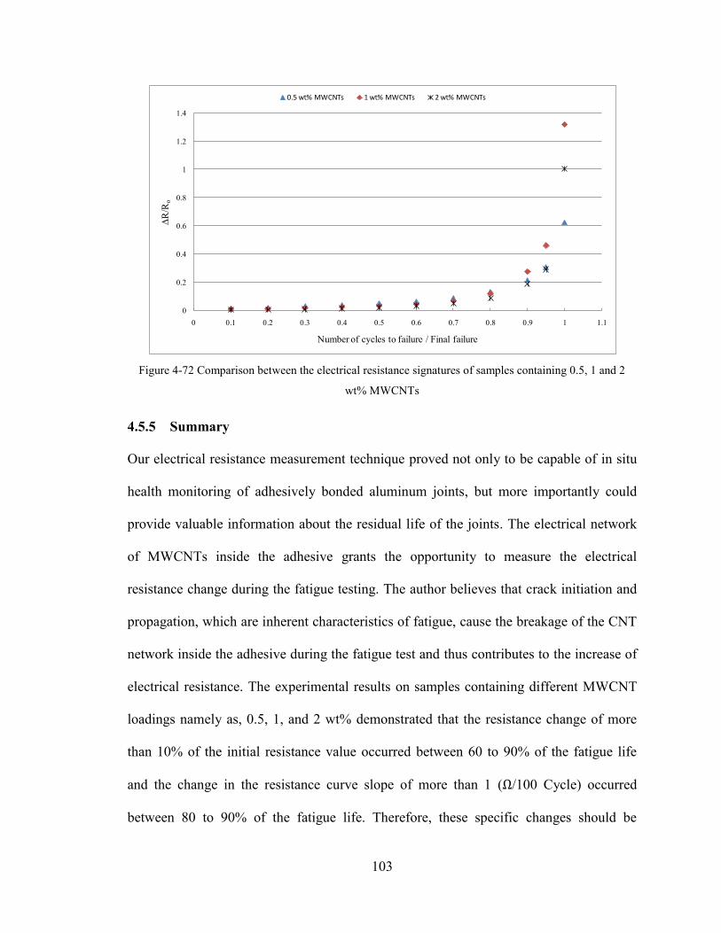
103
Figure 4-72 Comparison between the electrical resistance signatures of samples containing 0.5, 1 and 2
wt% MWCNTs
4.5.5 Summary
Our electrical resistance measurement technique proved not only to be capable of in situ
health monitoring of adhesively bonded aluminum joints, but more importantly could
provide valuable information about the residual life of the joints. The electrical network
of MWCNTs inside the adhesive grants the opportunity to measure the electrical
resistance change during the fatigue testing. The author believes that crack initiation and
propagation, which are inherent characteristics of fatigue, cause the breakage of the CNT
network inside the adhesive during the fatigue test and thus contributes to the increase of
electrical resistance. The experimental results on samples containing different MWCNT
loadings namely as, 0.5, 1, and 2 wt% demonstrated that the resistance change of more
than 10% of the initial resistance value occurred between 60 to 90% of the fatigue life
and the change in the resistance curve slope of more than 1 (Ω/100 Cycle) occurred
between 80 to 90% of the fatigue life. Therefore, these specific changes should be
0
0.2
0.4
0.6
0.8
1
1.2
1.4
0 0.1 0.2 0.3 0.4 0.5 0.6 0.7 0.8 0.9 1 1.1
∆R
/Ro
Number of cycles to failure / Final failure
0.5 wt% MWCNTs 1 wt% MWCNTs 2 wt% MWCNTs
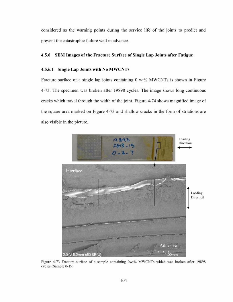
104
considered as the warning points during the service life of the joints to predict and
prevent the catastrophic failure well in advance.
4.5.6 SEM Images of the Fracture Surface of Single Lap Joints after Fatigue
4.5.6.1 Single Lap Joints with No MWCNTs
Fracture surface of a single lap joints containing 0 wt% MWCNTs is shown in Figure
4-73. The specimen was broken after 19898 cycles. The image shows long continuous
cracks which travel through the width of the joint. Figure 4-74 shows magnified image of
the square area marked on Figure 4-73 and shallow cracks in the form of striations are
also visible in the picture.
Figure 4-73 Fracture surface of a sample containing 0wt% MWCNTs which was broken after 19898
cycles.(Sample 0-19)
Loading
Direction
Loading
Direction
Interface
Adhesive
105
a)
b)
Figure 4-74 Magnified image of the square area marked on Figure 4-73, a) 500μm, b) 100 μm
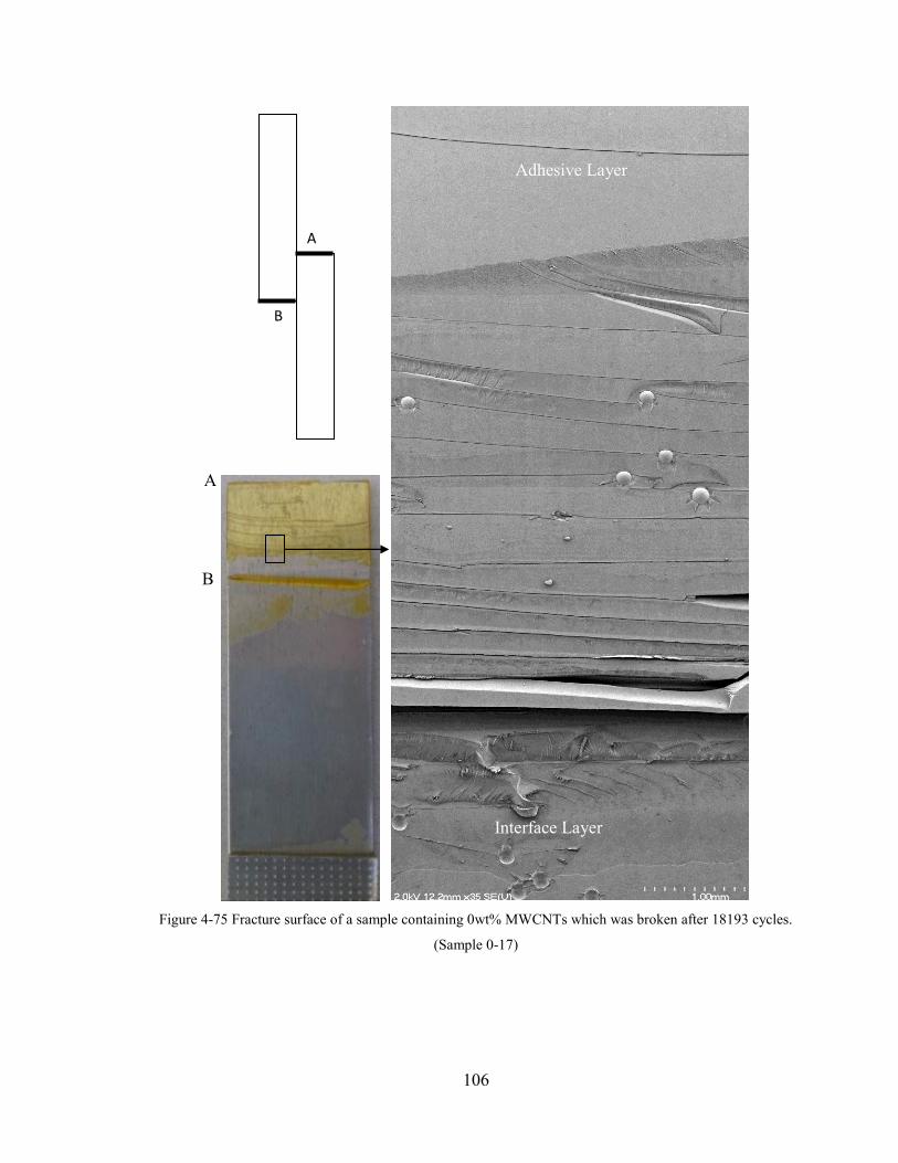
106
Figure 4-75 Fracture surface of a sample containing 0wt% MWCNTs which was broken after 18193 cycles.
(Sample 0-17)
A
B
A
B
Adhesive Layer
Interface Layer
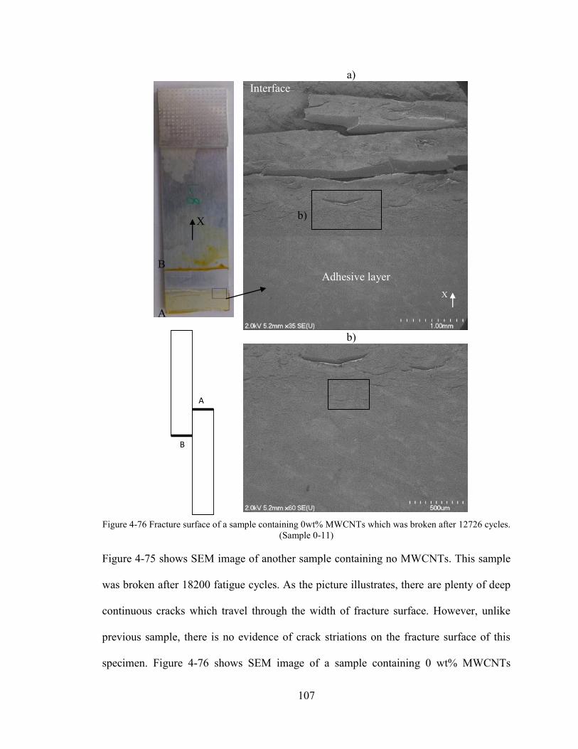
107
a)
b)
Figure 4-76 Fracture surface of a sample containing 0wt% MWCNTs which was broken after 12726 cycles.
(Sample 0-11)
Figure 4-75 shows SEM image of another sample containing no MWCNTs. This sample
was broken after 18200 fatigue cycles. As the picture illustrates, there are plenty of deep
continuous cracks which travel through the width of fracture surface. However, unlike
previous sample, there is no evidence of crack striations on the fracture surface of this
specimen. Figure 4-76 shows SEM image of a sample containing 0 wt% MWCNTs
A
B
A
B
Interface
Adhesive layer
X
b) X
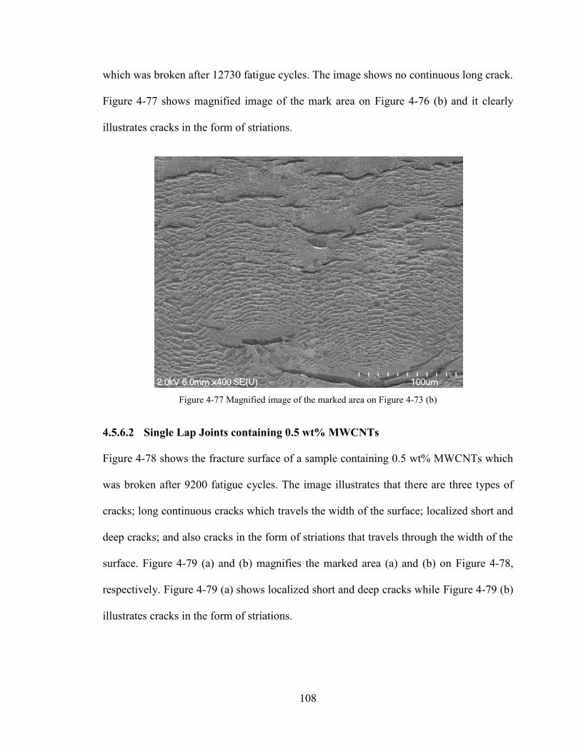
108
which was broken after 12730 fatigue cycles. The image shows no continuous long crack.
Figure 4-77 shows magnified image of the mark area on Figure 4-76 (b) and it clearly
illustrates cracks in the form of striations.
Figure 4-77 Magnified image of the marked area on Figure 4-73 (b)
4.5.6.2 Single Lap Joints containing 0.5 wt% MWCNTs
Figure 4-78 shows the fracture surface of a sample containing 0.5 wt% MWCNTs which
was broken after 9200 fatigue cycles. The image illustrates that there are three types of
cracks; long continuous cracks which travels the width of the surface; localized short and
deep cracks; and also cracks in the form of striations that travels through the width of the
surface. Figure 4-79 (a) and (b) magnifies the marked area (a) and (b) on Figure 4-78,
respectively. Figure 4-79 (a) shows localized short and deep cracks while Figure 4-79 (b)
illustrates cracks in the form of striations.
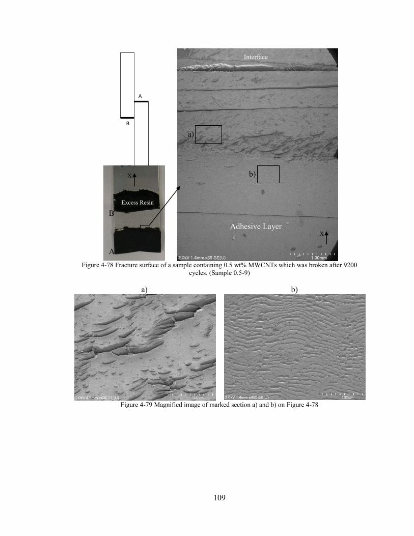
109
Figure 4-78 Fracture surface of a sample containing 0.5 wt% MWCNTs which was broken after 9200
cycles. (Sample 0.5-9)
a)
b)
Figure 4-79 Magnified image of marked section a) and b) on Figure 4-78
A
B
Excess Resin
B
A
a)
b) X
X Adhesive Layer
Interface
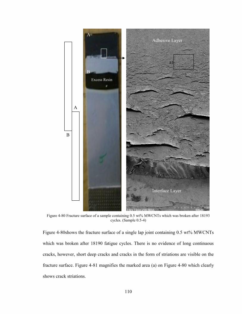
110
Figure 4-80 Fracture surface of a sample containing 0.5 wt% MWCNTs which was broken after 18193
cycles. (Sample 0.5-4)
Figure 4-80shows the fracture surface of a single lap joint containing 0.5 wt% MWCNTs
which was broken after 18190 fatigue cycles. There is no evidence of long continuous
cracks, however, short deep cracks and cracks in the form of striations are visible on the
fracture surface. Figure 4-81 magnifies the marked area (a) on Figure 4-80 which clearly
shows crack striations.
A
B
A
B
Excess Resin
Adhesive Layer
Interface Layer
a)
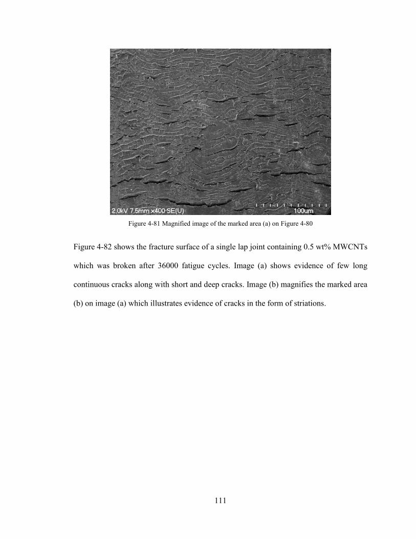
111
Figure 4-81 Magnified image of the marked area (a) on Figure 4-80
Figure 4-82 shows the fracture surface of a single lap joint containing 0.5 wt% MWCNTs
which was broken after 36000 fatigue cycles. Image (a) shows evidence of few long
continuous cracks along with short and deep cracks. Image (b) magnifies the marked area
(b) on image (a) which illustrates evidence of cracks in the form of striations.
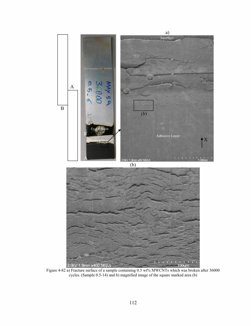
112
a)
(b)
Figure 4-82 a) Fracture surface of a sample containing 0.5 wt% MWCNTs which was broken after 36000
cycles. (Sample 0.5-14) and b) magnified image of the square marked area (b)
B
A
Adhesive Layer
A
B
X
Interface
(b)
Excess Resin
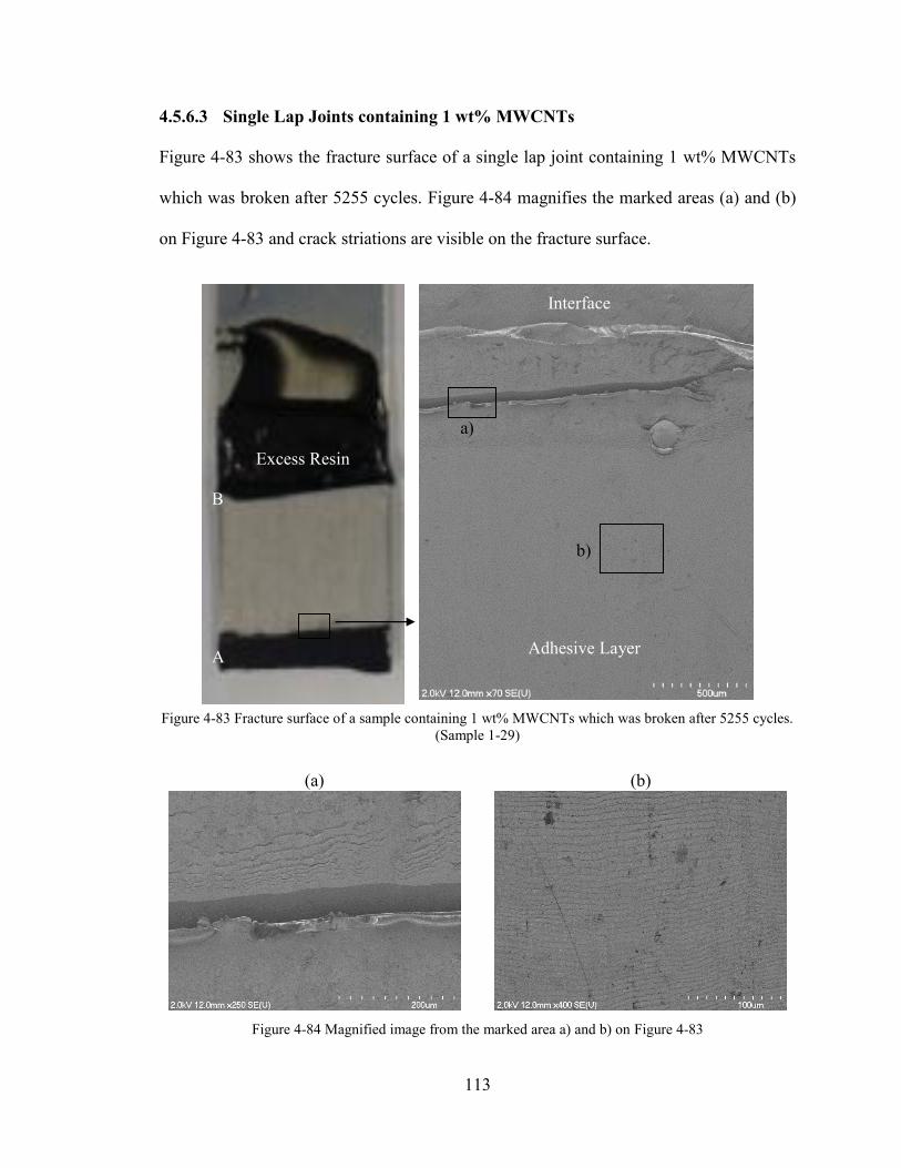
113
4.5.6.3 Single Lap Joints containing 1 wt% MWCNTs
Figure 4-83 shows the fracture surface of a single lap joint containing 1 wt% MWCNTs
which was broken after 5255 cycles. Figure 4-84 magnifies the marked areas (a) and (b)
on Figure 4-83 and crack striations are visible on the fracture surface.
Figure 4-83 Fracture surface of a sample containing 1 wt% MWCNTs which was broken after 5255 cycles.
(Sample 1-29)
(a)
(b)
Figure 4-84 Magnified image from the marked area a) and b) on Figure 4-83
Excess Resin
A
B
Adhesive Layer
Interface
a)
b)
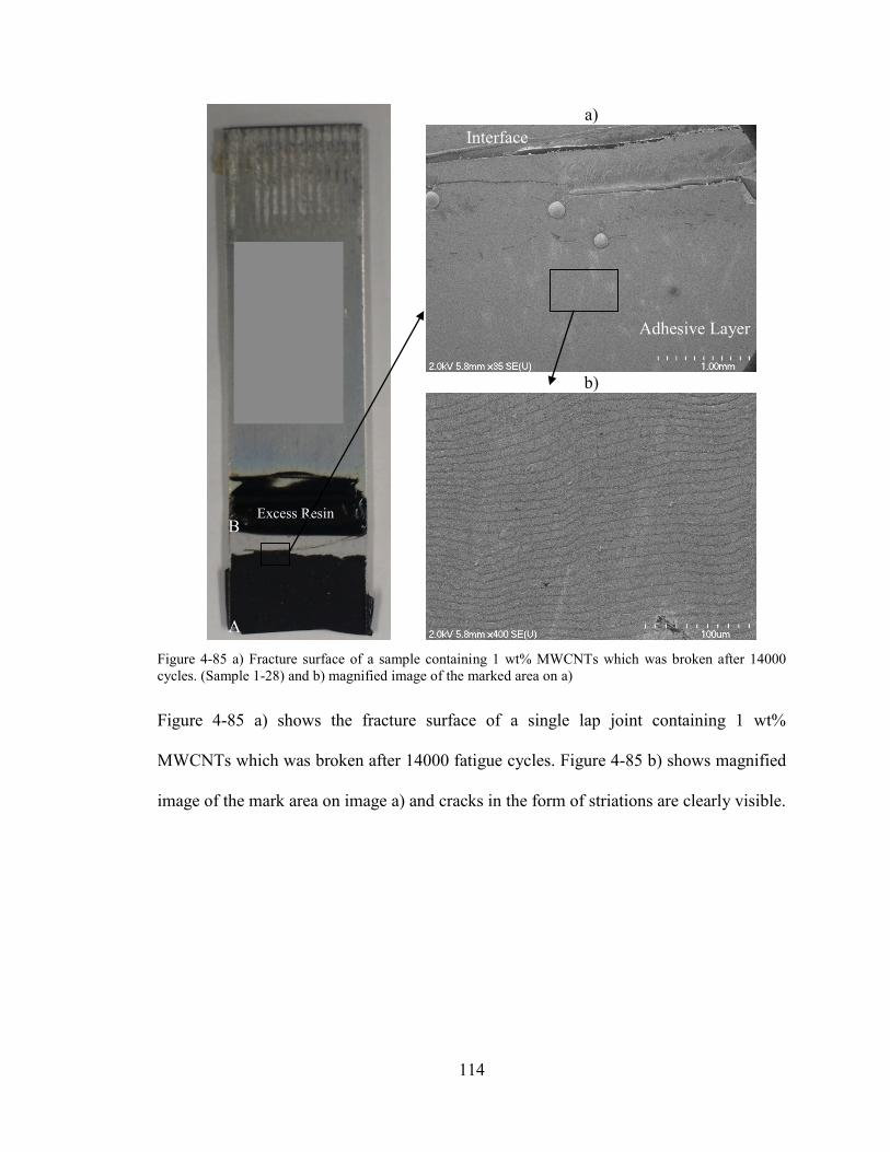
114
a)
b)
Figure 4-85 a) Fracture surface of a sample containing 1 wt% MWCNTs which was broken after 14000
cycles. (Sample 1-28) and b) magnified image of the marked area on a)
Figure 4-85 a) shows the fracture surface of a single lap joint containing 1 wt%
MWCNTs which was broken after 14000 fatigue cycles. Figure 4-85 b) shows magnified
image of the mark area on image a) and cracks in the form of striations are clearly visible.
Excess Resin
A
B
Interface
Adhesive Layer
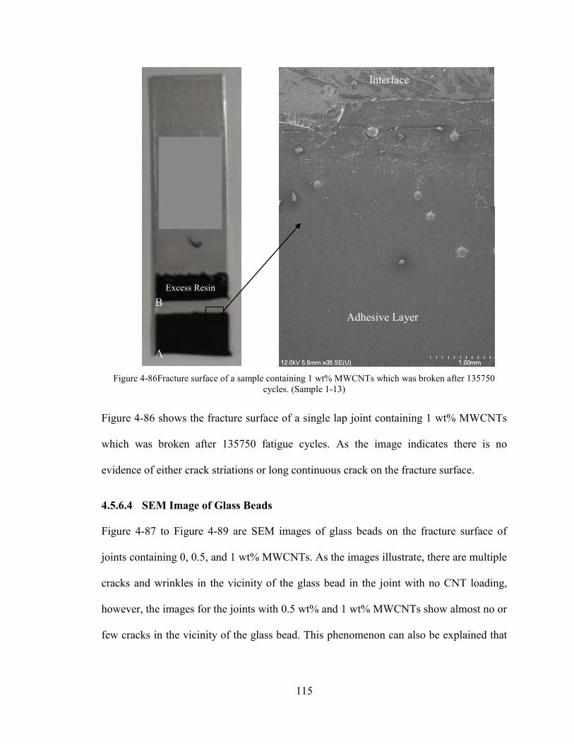
115
Figure 4-86Fracture surface of a sample containing 1 wt% MWCNTs which was broken after 135750
cycles. (Sample 1-13)
Figure 4-86 shows the fracture surface of a single lap joint containing 1 wt% MWCNTs
which was broken after 135750 fatigue cycles. As the image indicates there is no
evidence of either crack striations or long continuous crack on the fracture surface.
4.5.6.4 SEM Image of Glass Beads
Figure 4-87 to Figure 4-89 are SEM images of glass beads on the fracture surface of
joints containing 0, 0.5, and 1 wt% MWCNTs. As the images illustrate, there are multiple
cracks and wrinkles in the vicinity of the glass bead in the joint with no CNT loading,
however, the images for the joints with 0.5 wt% and 1 wt% MWCNTs show almost no or
few cracks in the vicinity of the glass bead. This phenomenon can also be explained that
Excess Resin
B
A
Adhesive Layer
Interface
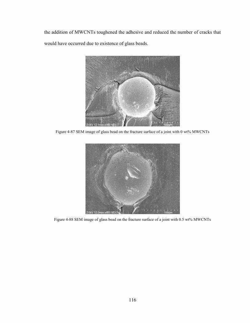
116
the addition of MWCNTs toughened the adhesive and reduced the number of cracks that
would have occurred due to existence of glass beads.
Figure 4-87 SEM image of glass bead on the fracture surface of a joint with 0 wt% MWCNTs
Figure 4-88 SEM image of glass bead on the fracture surface of a joint with 0.5 wt% MWCNTs
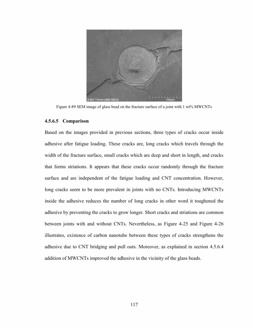
117
Figure 4-89 SEM image of glass bead on the fracture surface of a joint with 1 wt% MWCNTs
4.5.6.5 Comparison
Based on the images provided in previous sections, three types of cracks occur inside
adhesive after fatigue loading. These cracks are, long cracks which travels through the
width of the fracture surface, small cracks which are deep and short in length, and cracks
that forms striations. It appears that these cracks occur randomly through the fracture
surface and are independent of the fatigue loading and CNT concentration. However,
long cracks seem to be more prevalent in joints with no CNTs. Introducing MWCNTs
inside the adhesive reduces the number of long cracks in other word it toughened the
adhesive by preventing the cracks to grow longer. Short cracks and striations are common
between joints with and without CNTs. Nevertheless, as Figure 4-25 and Figure 4-26
illustrates, existence of carbon nanotube between these types of cracks strengthens the
adhesive due to CNT bridging and pull outs. Moreover, as explained in section 4.5.6.4
addition of MWCNTs improved the adhesive in the vicinity of the glass beads.
118
4.5.6.6 Conclusion
Author believes that a comprehensive study should be carried out in order to fully
understand the phenomenon described above. Further study on the fracture surface of
different joints with different CNT loading is recommended since, multiple factor can
affect the formation of cracks inside the adhesive. Some of these factors are, maximum
and minimum fatigue loading, frequency of the fatigue loading, different CNT
concentrations, different CNT types, and the fatigue cycle at which a specific joint is
broken.

119
Chapter 5
Conclusions and
Future Works

120
5 Conclusions and Future Works
5.1 Conclusions
Although adhesive joints have found application in aerospace and automotive industries,
lack of confidence in performing well under dynamic loadings may lead to reduction in
their usage on critical applications. Manager added confidence requires manufacturers to
add bolts or rivets to adhesive joints to bring confidence on their performance. In effect,
this manager added confidence leads to the structure to become heavy again. This
research projects introduced an in-situ monitoring technique which is capable of
evaluating the integrity of adhesively bonded joints and also provide valuable indicators
which predicts catastrophic failure well in advance. Application of this technique in real
structures can bring back the confidence in using adhesive joints in aerospace and
automotive industries.
On-line health monitoring and residual life prognosis using carbon nanotube networks
inside the adhesive proved to be capable of assessing the integrity of the joints throughout
dynamic loading. Three regions were observed on the electrical resistance signature
curve.
1. The safe zone which covered approximately 60% of the fatigue life. The
resistance increased linearly to less than 10% of the initial resistance.
2. The waning zone in which the resistance changes accelerated and reached to more
than 10% of the initial resistance.

121
3. The failure zone which indicates the final 10% of the fatigue life. The resistance
change was dramatic in this zone.
Moreover, two warning indicators were observed on the electrical resistance signatures of
adhesively bonded joints.
1. The resistance change of more than 10% of the joint initial resistance which
corresponded to the 60% to 90% of the fatigue life.
2. The slope of the resistance signature curve reached 1 (Ω/100 cycles) between 80
to 90% of the fatigue life.
This technique opened up a window in using adhesive joints with more confidence
regarding their fatigue behavior.
Comparison of adhesive joints with different MWCNTs loadings illustrates that addition
of 0.5 wt% CNTs increased the shear strength 10% compared to that of neat adhesive.
However, addition of more CNTs than 0.5 wt% did not have any significant effect on the
shear strength of the joints. Introducing 1 wt% MWCNTs improved the fatigue life of the
joints by more than 20% compared to neat adhesive. Electrical resistance dropped more
than 7 orders of magnitude by only dispersing 0.5 wt% MWCNTs inside adhesive resin.
5.2 Contribution
The main contribution of this project was introducing a structural health monitoring
technique to be used for adhesively bonded joints to increase their reliability throughout
their service life. Although adhesive joints have good fatigue behavior, catastrophic
failure without any warning is common between them. Therefore, it is necessary to

122
provide an in-situ technique to improve their reliability throughout dynamic loading. In
this research project the sensitivity of the carbon nanotube networks inside the adhesive
towards damages and cracks was used to evaluate the integrity of the joints and to predict
the failure well in advance. The probability to predict the catastrophic failure before it
occurs offers more confidence and reliability in the application of adhesive joints which
is of prime importance in aerospace and automotive industries. Therefore, improving the
reliability of adhesive joints to perform under dynamic loading is the most outstanding
outcome of this thesis project.
5.3 Future Works
The proposed technique is just a beginning of a journey to improve the reliability of
adhesive joints under dynamic loading. More has to be done to create a complete
technique to monitor the integrity of adhesive bonds and predict their failure under all
real life circumstances. Long term effects of moisture, temperature, relaxation, and
corrosion should be investigated on adhesive bonds and in effect the capability of the
technique to perform well under these effects should be evaluated. A theoretical model
based on this technique should be generated to complement the experimental results and
to present insight into the fatigue behavior of adhesively bonded joints. Therefore, more
experiments on different joint geometry in different loading conditions should be
performed to produce a complete data archive on the fatigue life of adhesively bonded
joints. Hence the data archive should be used to generate a comprehensive theoretical
model along with a complete in-situ technique to provide accurate residual life prognosis
under complex real life conditions.

123
6 References
1. Zhang W., Sakalkar V., and Koratkar N., "In Situ Health Monitoring and Repair in Composites using Carbon
Nanotube Additives," Applied Physics Letters, 2007, 91(13) pp. 133102.
2. KahramanRamazan, Sunar Mehmet, and YilbasBekir, "Influence of Adhesive Thickness and Filler Content on
the Mechanical Performance of Aluminum Single-Lap Joints Bonded with Aluminum Powder Filled Epoxy
Adhesive," Journal of Materials Processing Technology, 2008, 205(1-3) pp. 183-189.
3. Borsellino C., Di Bella G., and Ruisi V. F., "Adhesive Joining of Aluminium AA6082: The Effects of Resin
and Surface Treatment," International Journal of Adhesion and Adhesives, 2009, 29(1) pp. 36-44.
4. Pereira, A. M., Ferreira, J. M., Antunes, F. V., and Bártolo, P. J., "Study on the Fatigue Strength of AA 6082-
T6 Adhesive Lap Joints," International Journal of Adhesion and Adhesives, 2009, 29(6) pp. 633-638.
5. M PEREIRA A. M FERREIRA J. V ANTUNES F., and J BARTOLO P., "Analysis of Manufacturing
Parameters on the Shear Strength of Aluminium Adhesive Single-Lap Joints," 2010, 210(4) pp. 610; 8-617.
6. Jen Yi-Ming, and KoChih-Wei, "Evaluation of Fatigue Life of Adhesively Bonded Aluminum Single-Lap
Joints using Interfacial Parameters," International Journal of Fatigue, 2010, 32(2) pp. 330-340.
7. Barnes T. A., and Pashby I. R., "Joining Techniques for AluminiumSpaceframes used in Automobiles: Part II
— Adhesive Bonding and Mechanical Fasteners," Journal of Materials Processing Technology, 2000, 99(1-3)
pp. 72-79.
8. Mollie A. Bily, Young W. Kwon, Randall D. Pollak, "Technical Report Naval Postgraduate School: Damage
Detection in Composite Interfaces Through Carbon Nanotube Reinforcement." 2010.
9. Daniel Balageas, Claus-Peter Fritzen, Alfredo Guemes, "Structural Health Monitoring," ISTE Ltd,2006.
10. Baldev Raj, T. Jayakumar, M. Thavasimuthu, "Practical non-destructive testing," 2007, Oxford, U.K. :
Alpha Science Internationa, U.K., .
11. Gros X. E. (Xavier Emanuel), "NDT data fusion / X.E. Gros." Elsevier Science Ltd,1997, .
12. Prolongo S. G., Gude M. R., Sanchez J., and UreÃa A., "Nanoreinforced Epoxy Adhesives for Aerospace
Industry," The Journal of Adhesion, 2009, 85(4-5) pp. 180-199.
13. Thostenson Erik T., and ChouTsu-Wei, "Carbon Nanotube-Based Health Monitoring of Mechanically
Fastened Composite Joints," Composites Science and Technology, 2008, 68(12) pp. 2557-2561.
14. BiernackiJacek M., and Beall Frank C., "Acoustic Monitoring of Cold-Setting Adhesive Curing in Wood
Laminates," International Journal of Adhesion and Adhesives, 1996, 16(3) pp. 165-172.
124
15. Yang Shuo, GuLan, and Gibson Ronald F., "Nondestructive Detection of Weak Joints in Adhesively Bonded
Composite Structures," Composite Structures, 2001, 51(1) pp. 63-71.
16. MICKENS T., SCHULZ M., SUNDARESAN M., GHOSHAL A., NASER A. S., and REICHMEIDER R.,
"STRUCTURAL HEALTH MONITORING OF AN AIRCRAFT JOINT," Mechanical Systems and Signal
Processing, 2003, 17(2) pp. 285-303.
17. Jones R., and Galea S., "Health Monitoring of Composite Repairs and Joints using Optical Fibres,"
Composite Structures, 2002, 58(3) pp. 397-403.
18. Brotherhood C. J., Drinkwater B. W., and Dixon S., "The Detectability of Kissing Bonds in Adhesive Joints
using Ultrasonic Techniques," Ultrasonics, 2003, 41(7) pp. 521-529.
19. Herszberg I., Li H. C. H., Dharmawan F., Mouritz A. P., Nguyen M., and Bayandor J., "Damage Assessment
and Monitoring of Composite Ship Joints," Composite Structures, 2005, 67(2) pp. 205-216.
20. Kesavan A., Deivasigamani M., John S., and Herszberg I., "Damage Detection in T-Joint Composite
Structures," Composite Structures, 2006, 75(1-4) pp. 313-320.
21. Palaniappan J., Wang H., Ogin S. L., Thorne A. M., Reed G. T., Crocombe A. D., Rech Y., and Tjin S. C.,
"Changes in the Reflected Spectra of Embedded Chirped Fibre Bragg Gratings used to Monitor Disbonding
in Bonded Composite Joints," Composites Science and Technology, 2007, 67(13) pp. 2847-2853.
22. Palaniappan J., Ogin S. L., Thorne A. M., Reed G. T., Crocombe A. D., Capell T. F., Tjin S. C., and Mohanty
L., "Disbond Growth Detection in composite–composite Single-Lap Joints using Chirped FBG Sensors,"
Composites Science and Technology, 2008, 68(12) pp. 2410-2417.
23. Karp Baruch, Rittel Daniel, and Durban David, "Health Monitoring of Joints using Dynamic End Effects,"
Journal of Sound and Vibration, 2008, 312(1-2) pp. 257-272.
24. Zhang Ye, Vassilopoulos, Anastasios P., and Keller Thomas, "Stiffness Degradation and Fatigue Life
Prediction of Adhesively-Bonded Joints for Fiber-Reinforced Polymer Composites," International Journal of
Fatigue, 2008, 30(10-11) pp. 1813-1820.
25. VotsisRenosA., and ChryssanthopoulosMarios K., "Assessment of Debonding in GFRP Joints using Damage
Identification Techniques," Construction and Building Materials, 2009, 23(4) pp. 1690-1697.
26. Fasel Timothy R., and Todd Michael D., "An Adhesive Bond State Classification Method for a Composite
Skin-to-Spar Joint using Chaotic Insonification," Journal of Sound and Vibration, 2010, 329(15) pp. 3218-
3232.
27. Fasel T. R., and Todd M. D., "Chaotic Insonification for Health Monitoring of an Adhesively Bonded
Composite Stiffened Panel," Mechanical Systems and Signal Processing, 2010, 24(5) pp. 1420-1430.
125
28. Argatov Ivan, and Sevostianov Igor, "Health Monitoring of Bolted Joints Via Electrical Conductivity
Measurements," International Journal of Engineering Science, 2010, 48(10) pp. 874-887.
29. Balle Frank, Huxhold Stefan, Wagner Guntram, and EiflerDietmar, "Damage Monitoring of Ultrasonically
Welded Aluminum/ CFRP-Joints by Electrical Resistance Measurements," Procedia Engineering, 2011, 10pp.
433-438.
30. Bernasconi Andrea, Carboni Michele, and Comolli Lorenzo, "Monitoring of Fatigue Crack Growth in
Composite Adhesively Bonded Joints using Fiber Bragg Gratings," Procedia Engineering, 2011, 10pp. 207-
212.
31. BrankoGlisicI., "Fiber Optic Methods For Structural Health Monitoring," John Wiley & Sons Ltd.2007, .
32. Kroto H. W., Heath J. R., O'Brien S. C., Curl R. F., and Smalley R. E., "C60: Buckminsterfullerene," Nature,
1985, 318(6042) pp. 162-163.
33. IijimaSumio, "Helical Microtubules of Graphitic Carbon," Nature, 1991, 354(6348) pp. 56-58.
34. Thostenson Erik T., Li Chunyu, and ChouTsu-Wei, "Nanocomposites in Context," Composites Science and
Technology, 2005, 65(3-4) pp. 491-516.
35. T THOSTENSON E., REN ZHIFENG, and Tsu-Wei CHOU, "Advances in the Science and Technology of
Carbon Nanotubes and their Composites : A Review," 2001, 61(13) pp. 1899-1912.
36. EsawiAmal M. K., and Farag Mahmoud M., "Carbon Nanotube Reinforced Composites: Potential and
Current Challenges," Materials & Design, 2007, 28(9) pp. 2394-2401.
37. Breuer O., and SundararajUttandaraman, "Big Returns from Small Fibers: A Review of polymer/carbon
Nanotube Composites," Polymer Composites, 2004, 25(6) pp. 630-645.
38. Jing Li, and Lumpp J. K., 2007, "Carbon Nanotube Filled Conductive Adhesives for Aerospace
Applications," Aerospace Conference, 2007 IEEE, Anonymous pp. 1-6.
39. SihnSangwook, GanguliSabyasachi, Roy Ajit K., QuLiangti, and Dai Liming, "Enhancement of through-
Thickness Thermal Conductivity in Adhesively Bonded Joints using Aligned Carbon Nanotubes," Composites
Science and Technology, 2008, 68(3-4) pp. 658-665.
40. Yu Suzhu, Tong Min N., and Critchlow Gary, "Use of Carbon Nanotubes Reinforced Epoxy as Adhesives to
Join Aluminum Plates," Materials & Design, 2010, 31(Supplement 1) pp. S126-S129.
41. Gojny Florian H., WichmannMalte H. G., Fiedler Bodo, and Schulte Karl, "Influence of Different Carbon
Nanotubes on the Mechanical Properties of Epoxy Matrix Composites – A Comparative Study," Composites
Science and Technology, 2005, 65(15-16) pp. 2300-2313.
126
42. Yu Suzhu, Tong Min N., and Critchlow Gary, "Wedge Test of Carbon-Nanotube-Reinforced Epoxy Adhesive
Joints," Journal of Applied Polymer Science, 2009, 111(6) pp. 2957-2962.
43. Xu L. R., Li Lang, Lukehart Charles M., and KuaiHuacheng, "Mechanical Characterization of Nanofiber-
Reinforced Composite Adhesives," Journal of Nanoscience and Nanotechnology, 2007, 7(7) pp. 2546-2548.
44. Wu H. P., Wu X. J., Ge M. Y., Zhang G. Q., Wang Y. W., and JiangJianzhong, "Properties Investigation on
Isotropical Conductive Adhesives Filled with Silver Coated Carbon Nanotubes," Composites Science and
Technology, 2007, 67(6) pp. 1182-1186.
45. Kuang-Ting Hsiao, Justin Alms, and Suresh G Advani, "Use of epoxy/multiwalled Carbon Nanotubes as
Adhesives to Join Graphite Fibre Reinforced Polymer Composites," Nanotechnology, 2003, 14(7) pp. 791.
46. Baughman Ray H., Cui Changxing, ZakhidovAnvar A., IqbalZafar, Barisci Joseph N., Spinks Geoff M.,
Wallace Gordon G., Mazzoldi Alberto, De Rossi Danilo, Rinzler Andrew G., Jaschinski Oliver, Roth
Siegmar, and KerteszMiklos, "Carbon Nanotube Actuators," Science, 1999, 284(5418) pp. 1340-1344.
47. Li Chunyu, and ChouTsu-Wei, "Atomistic Modeling of Carbon Nanotube-Based Mechanical Sensors,"
Journal of Intelligent Material Systems and Structures, 2006, 17(3) pp. 247-254.
48. Thostenson E. T., and Chou Tsu-Wei, "Carbon Nanotube Networks: Sensing of Distributed Strain and
Damage for Life Prediction and Self Healing," Advanced Materials, 2006, 18(21) pp. 2837-2841.
49. Nofar M., Hoa S. V., and Pugh M. D., "Failure Detection and Monitoring in Polymer Matrix Composites
Subjected to Static and Dynamic Loads using Carbon Nanotube Networks," Composites Science and
Technology, 2009, 69(10) pp. 1599-1606.
50. GaoLimin, Thostenson Erik T., Zhang Zuoguang, and ChouTsu-Wei, "Sensing of Damage Mechanisms in
Fiber-Reinforced Composites Under Cyclic Loading using Carbon Nanotubes," Advanced Functional
Materials, 2009, 19(1) pp. 123-130.
51. Lim Amanda S., Melrose Zachary R., Thostenson Erik T., and ChouTsu-Wei, "Damage Sensing of
Adhesively-Bonded Hybrid composite/steel Joints using Carbon Nanotubes," Composites Science and
Technology, 2011, 71(9) pp. 1183-1189.
52. RoscaIosif D., and HoaSuong V., "Highly Conductive Multiwall Carbon Nanotube and Epoxy Composites
Produced by Three-Roll Milling," Carbon, 2009, 47(8) pp. 1958-1968.
53. Pereira A. M., Ferreira J. M., Antunes F. V., and Bártolo P. J., "Study on the Fatigue Strength of AA 6082-T6
Adhesive Lap Joints," International Journal of Adhesion and Adhesives, 2009, 29(6) pp. 633-638.

127
54. Liang Zhiyong, GouJihua, Zhang Chuck, Wang Ben, and Kramer Leslie, "Investigation of Molecular
Interactions between (10, 10) Single-Walled Nanotube and Epon 862 resin/DETDA Curing Agent
Molecules," Materials Science and Engineering A, 2004, 365(1-2) pp. 228-234.
55. Nagy Peter B., "Ultrasonic Classification of Imperfect Interfaces," Journal of Nondestructive Evaluation,
1992, 11(3) pp. 127-139.
56. http://asm.matweb.com
57. http://www.hexion.com
58. http://www.cheaptubesinc.com/MWNTs.htm
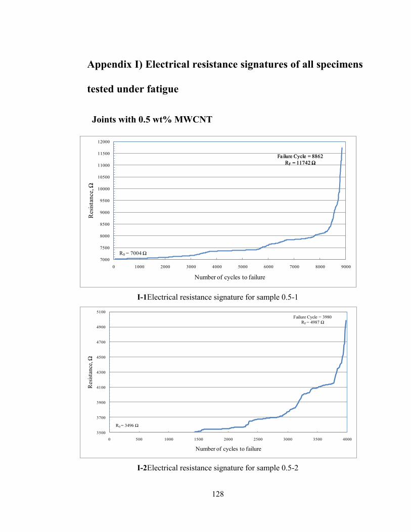
128
Appendix I) Electrical resistance signatures of all specimens
tested under fatigue
Joints with 0.5 wt% MWCNT
I-1Electrical resistance signature for sample 0.5-1
I-2Electrical resistance signature for sample 0.5-2
R0 = 7004 Ω
7000
7500
8000
8500
9000
9500
10000
10500
11000
11500
12000
0 1000 2000 3000 4000 5000 6000 7000 8000 9000
Res
ista
nce
, Ω
Number of cycles to failure
Failure Cycle = 8862
RF = 11742 Ω
Failure Cycle = 8862
RF = 11742 Ω
R0 = 3496 Ω
Failure Cycle = 3980
RF = 4987 Ω
3500
3700
3900
4100
4300
4500
4700
4900
5100
0 500 1000 1500 2000 2500 3000 3500 4000
Res
ista
nce
, Ω
Number of cycles to failure
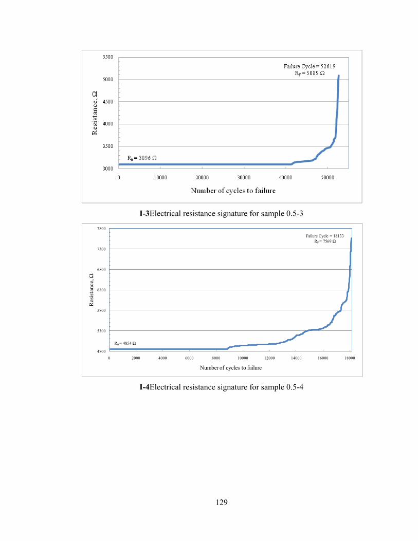
129
I-3Electrical resistance signature for sample 0.5-3
I-4Electrical resistance signature for sample 0.5-4
R0 = 4854 Ω
Failure Cycle = 18133
RF = 7569 Ω
4800
5300
5800
6300
6800
7300
7800
0 2000 4000 6000 8000 10000 12000 14000 16000 18000
Resi
stan
ce, Ω
Number of cycles to failure
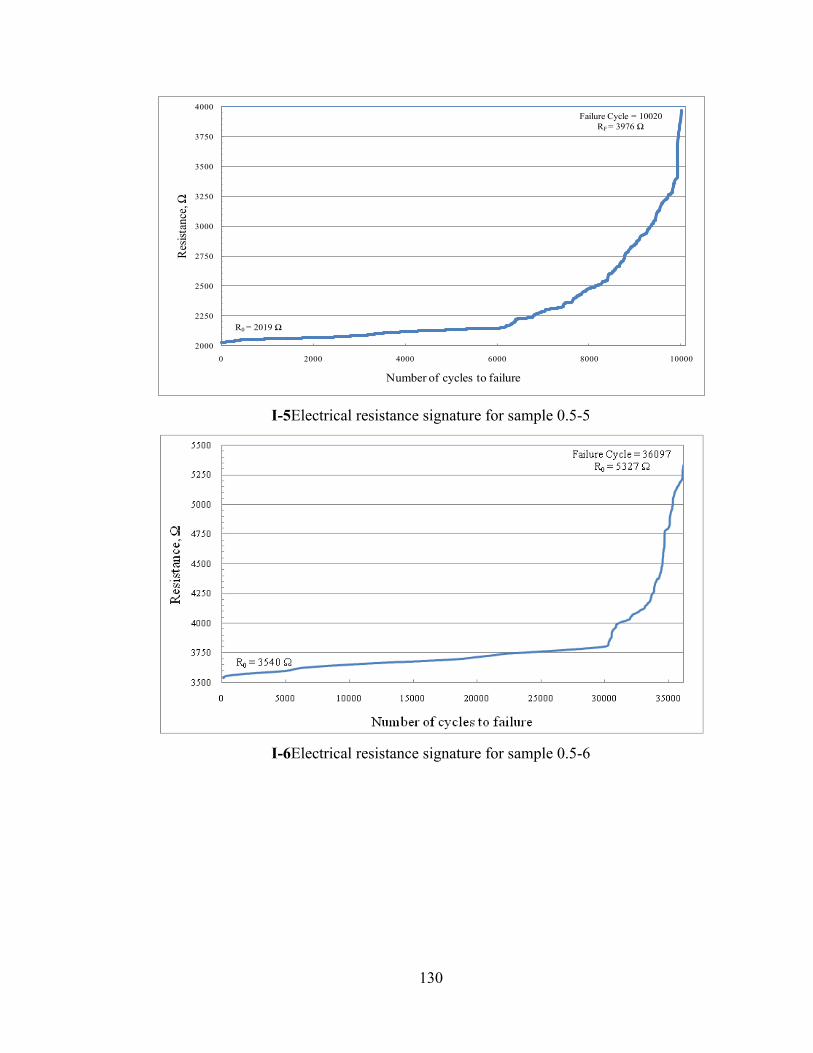
130
I-5Electrical resistance signature for sample 0.5-5
I-6Electrical resistance signature for sample 0.5-6
R0 = 2019 Ω
Failure Cycle = 10020
RF = 3976 Ω
2000
2250
2500
2750
3000
3250
3500
3750
4000
0 2000 4000 6000 8000 10000
Res
ista
nce
, Ω
Number of cycles to failure
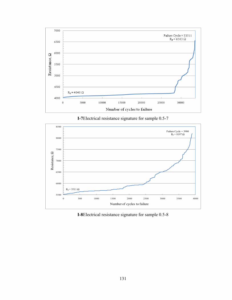
131
I-7Electrical resistance signature for sample 0.5-7
I-8Electrical resistance signature for sample 0.5-8
R0 = 5511 Ω
Failure Cycle = 3900
RF = 8197 Ω
5500
6000
6500
7000
7500
8000
8500
0 500 1000 1500 2000 2500 3000 3500 4000
Res
ista
nce
, Ω
Number of cycles to failure
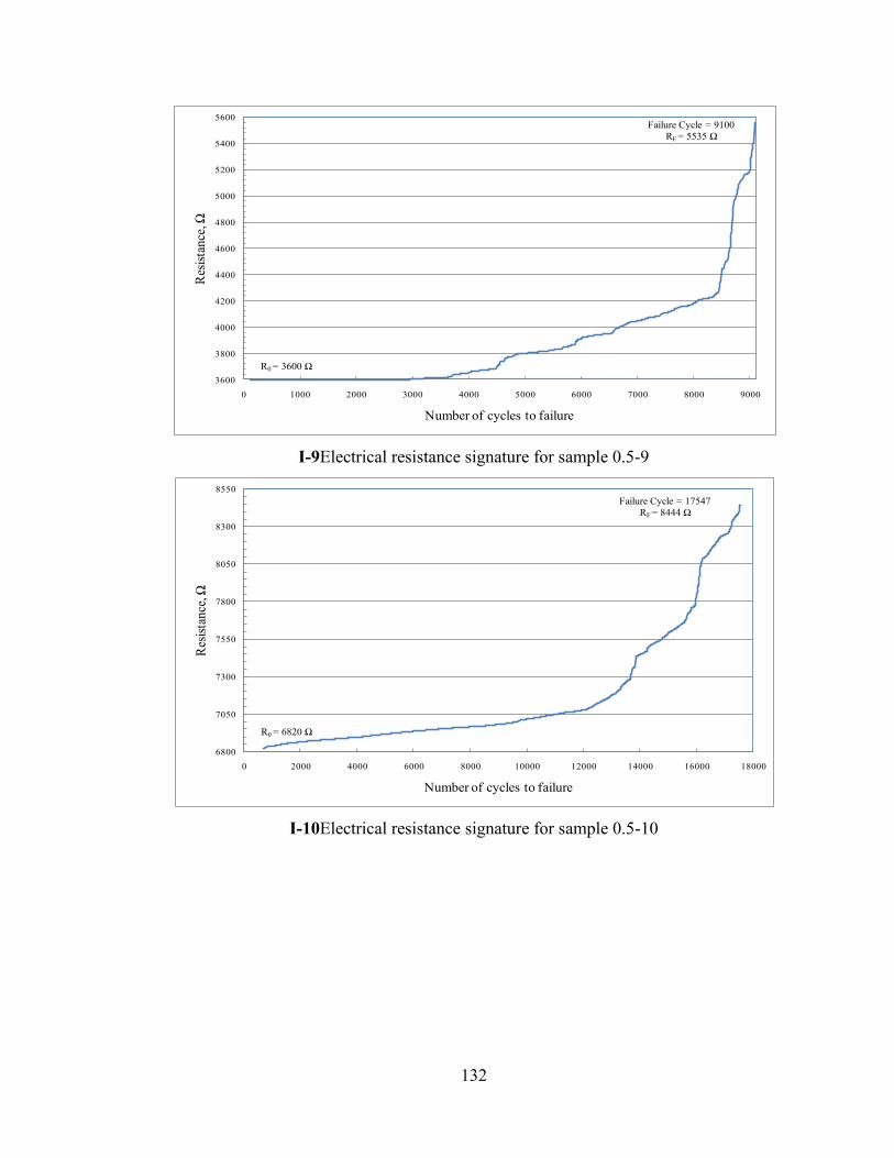
132
I-9Electrical resistance signature for sample 0.5-9
I-10Electrical resistance signature for sample 0.5-10
R0 = 3600 Ω
Failure Cycle = 9100
RF = 5535 Ω
3600
3800
4000
4200
4400
4600
4800
5000
5200
5400
5600
0 1000 2000 3000 4000 5000 6000 7000 8000 9000
Res
ista
nce
, Ω
Number of cycles to failure
R0 = 6820 Ω
Failure Cycle = 17547
RF = 8444 Ω
6800
7050
7300
7550
7800
8050
8300
8550
0 2000 4000 6000 8000 10000 12000 14000 16000 18000
Res
ista
nce
, Ω
Number of cycles to failure

133
I-11Electrical resistance signature for sample 0.5-11
I-12Electrical resistance signature for sample 0.5-12
R0 =3858 Ω
Failure Cycle = 12210
RF = 8773 Ω
3800
4800
5800
6800
7800
8800
0 2000 4000 6000 8000 10000 12000
Res
ista
nce
, Ω
Number of cycles to failure
R0 =7598 Ω
Failure Cycle = 11200
RF = 10719 Ω
7500
8000
8500
9000
9500
10000
10500
11000
0 2000 4000 6000 8000 10000
Res
ista
nce
, Ω
Number of cycles to failure
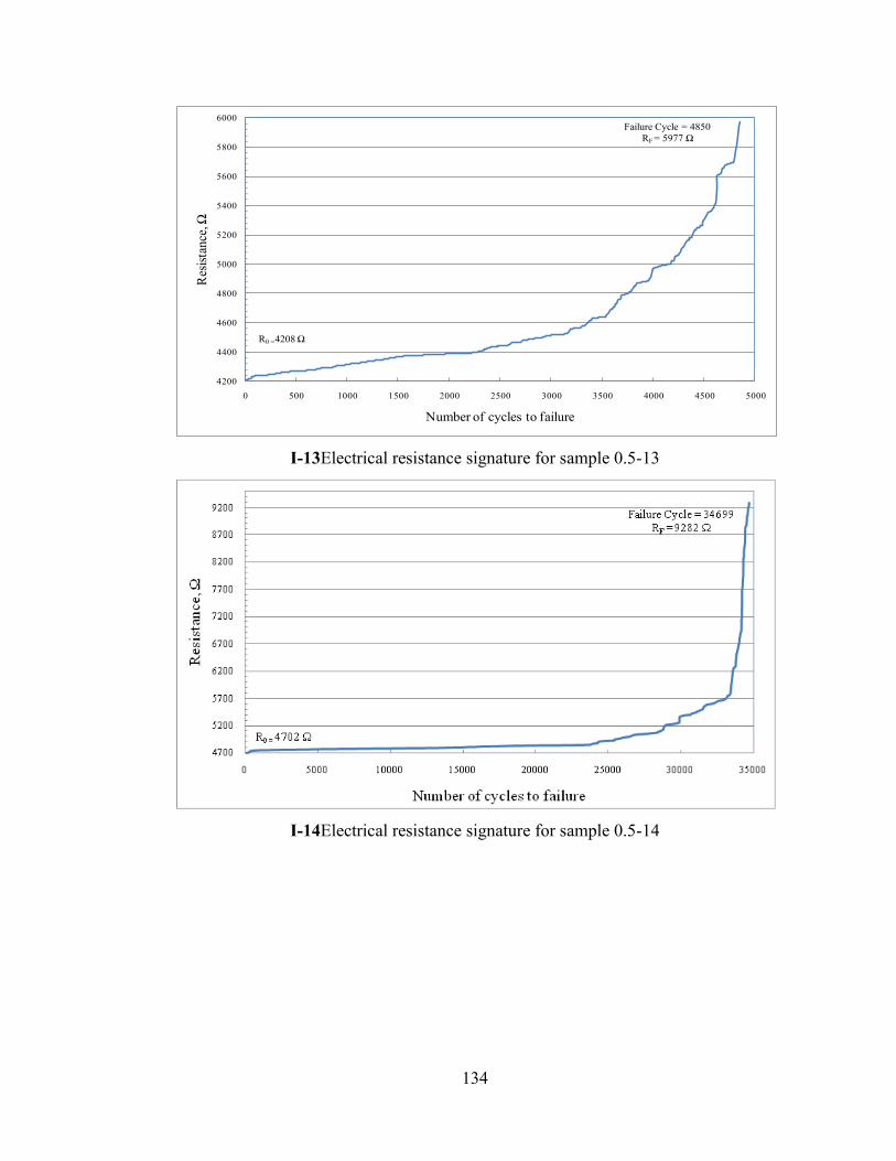
134
I-13Electrical resistance signature for sample 0.5-13
I-14Electrical resistance signature for sample 0.5-14
R0 =4208 Ω
Failure Cycle = 4850
RF = 5977 Ω
4200
4400
4600
4800
5000
5200
5400
5600
5800
6000
0 500 1000 1500 2000 2500 3000 3500 4000 4500 5000
Res
ista
nce
, Ω
Number of cycles to failure
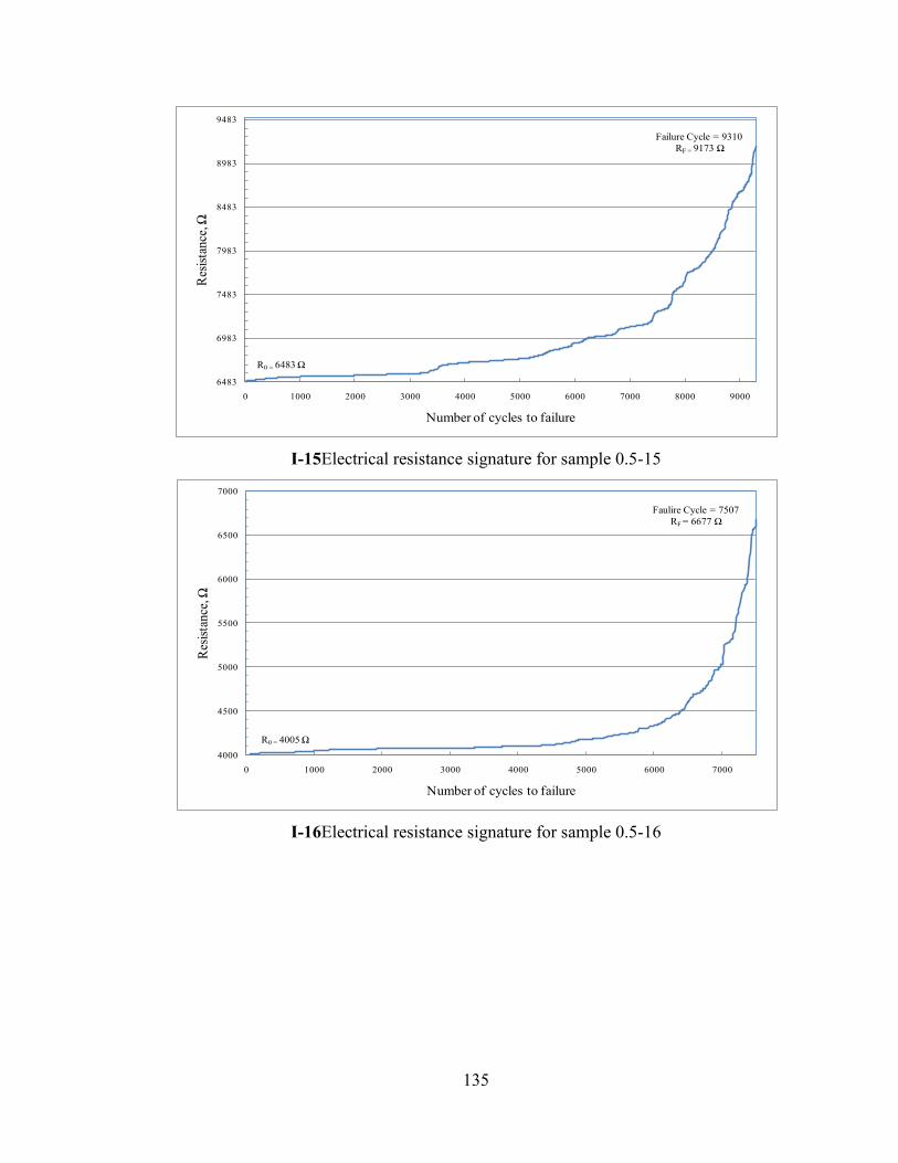
135
I-15Electrical resistance signature for sample 0.5-15
I-16Electrical resistance signature for sample 0.5-16
R0 = 6483 Ω
Failure Cycle = 9310
RF = 9173 Ω
6483
6983
7483
7983
8483
8983
9483
0 1000 2000 3000 4000 5000 6000 7000 8000 9000
Res
ista
nce
, Ω
Number of cycles to failure
R0 = 4005 Ω
Faulire Cycle = 7507
RF = 6677 Ω
4000
4500
5000
5500
6000
6500
7000
0 1000 2000 3000 4000 5000 6000 7000
Res
ista
nce
, Ω
Number of cycles to failure
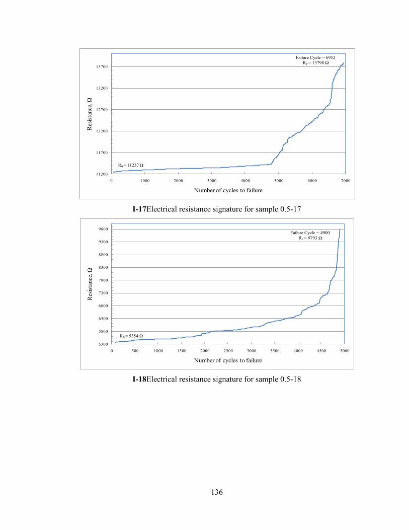
136
I-17Electrical resistance signature for sample 0.5-17
I-18Electrical resistance signature for sample 0.5-18
R0 = 11237 Ω
Failure Cycle = 6952
RF = 13798 Ω
11200
11700
12200
12700
13200
13700
0 1000 2000 3000 4000 5000 6000 7000
Res
ista
nce
, Ω
Number of cycles to failure
R0 = 5354 Ω
Failure Cycle = 4900
RF = 9793 Ω
5300
5800
6300
6800
7300
7800
8300
8800
9300
9800
0 500 1000 1500 2000 2500 3000 3500 4000 4500 5000
Res
ista
nce
, Ω
Number of cycles to failure
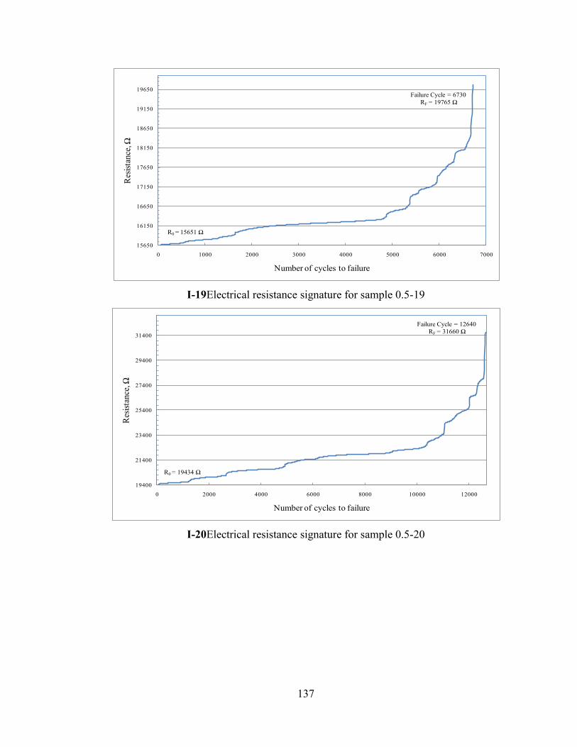
137
I-19Electrical resistance signature for sample 0.5-19
I-20Electrical resistance signature for sample 0.5-20
R0 = 15651 Ω
Failure Cycle = 6730
RF = 19765 Ω
15650
16150
16650
17150
17650
18150
18650
19150
19650
0 1000 2000 3000 4000 5000 6000 7000
Res
ista
nce
, Ω
Number of cycles to failure
R0 = 19434 Ω
Failure Cycle = 12640
RF = 31660 Ω
19400
21400
23400
25400
27400
29400
31400
0 2000 4000 6000 8000 10000 12000
Res
ista
nce
, Ω
Number of cycles to failure
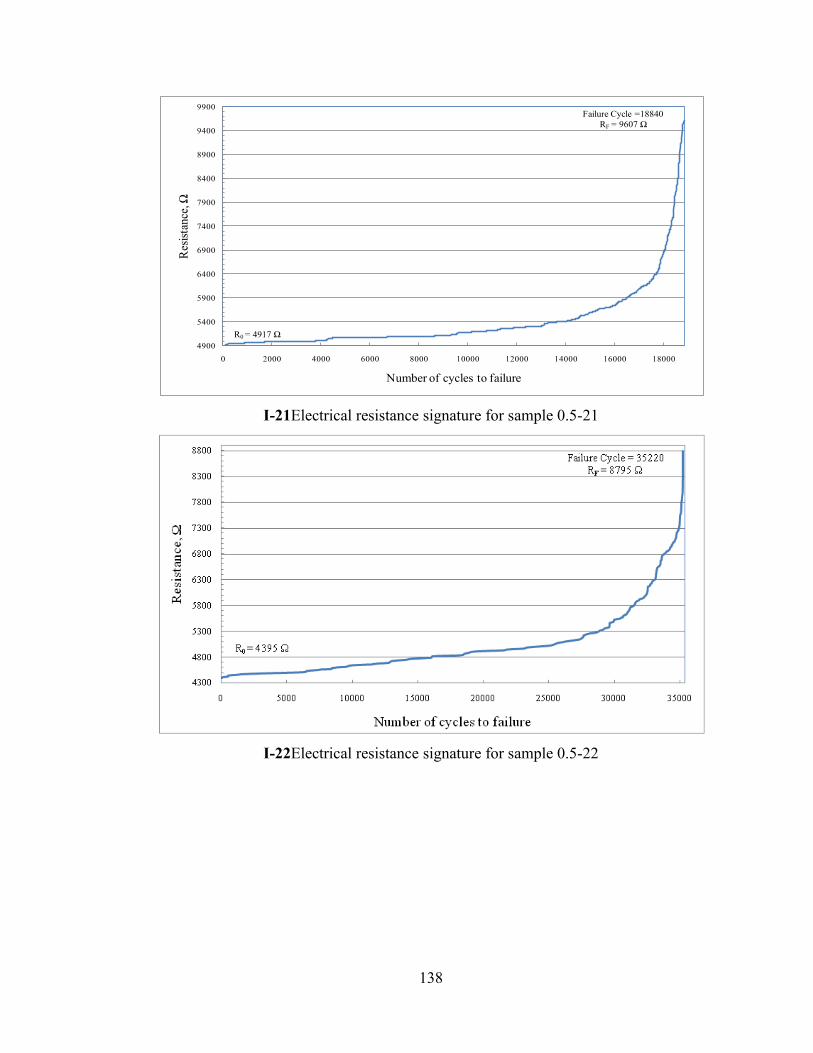
138
I-21Electrical resistance signature for sample 0.5-21
I-22Electrical resistance signature for sample 0.5-22
R0 = 4917 Ω
Failure Cycle =18840
RF = 9607 Ω
4900
5400
5900
6400
6900
7400
7900
8400
8900
9400
9900
0 2000 4000 6000 8000 10000 12000 14000 16000 18000
Res
ista
nce
, Ω
Number of cycles to failure
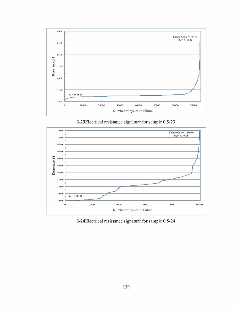
139
I-23Electrical resistance signature for sample 0.5-23
I-24Electrical resistance signature for sample 0.5-24
R0 = 3688 Ω
Failure Cycle = 73470
RF = 6161 Ω
3600
4100
4600
5100
5600
6100
6600
0 10000 20000 30000 40000 50000 60000 70000
Res
ista
nce
, Ω
Number of cycles to failure
R0 = 5300 Ω
Failure Cycle = 10040
RF = 7275 Ω
5300
5500
5700
5900
6100
6300
6500
6700
6900
7100
7300
0 2000 4000 6000 8000 10000
Res
ista
nce
, Ω
Number of cycles to failure
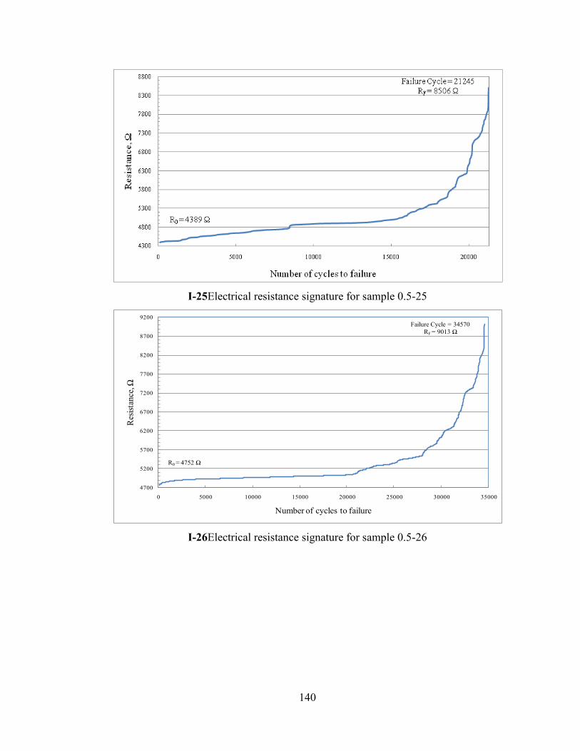
140
I-25Electrical resistance signature for sample 0.5-25
I-26Electrical resistance signature for sample 0.5-26
R0 = 4752 Ω
Failure Cycle = 34570
RF = 9013 Ω
4700
5200
5700
6200
6700
7200
7700
8200
8700
9200
0 5000 10000 15000 20000 25000 30000 35000
Res
ista
nce
, Ω
Number of cycles to failure

141
I-27Electrical resistance signature for sample 0.5-27
I-28Electrical resistance signature for sample 0.5-28
R0 = 6325 Ω
Failure Cycle = 10020
RF = 10594 Ω
6300
6800
7300
7800
8300
8800
9300
9800
10300
10800
0 2000 4000 6000 8000 10000
Res
ista
nce
, Ω
Number of cycles to failure
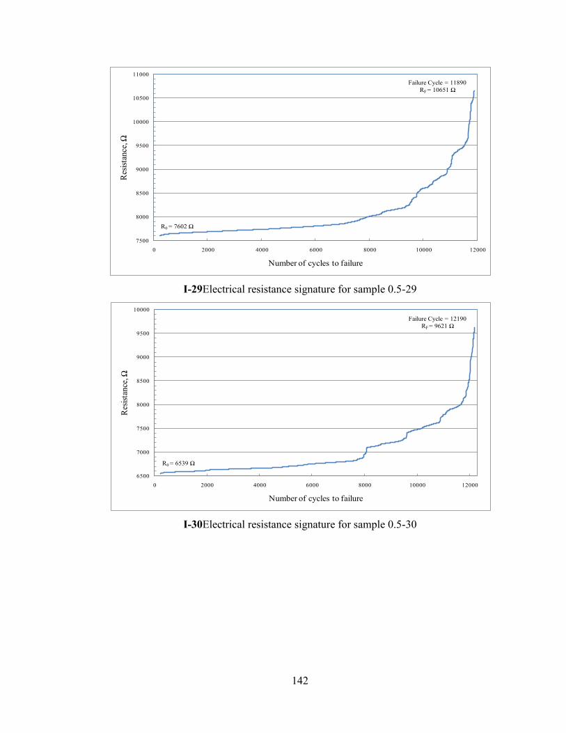
142
I-29Electrical resistance signature for sample 0.5-29
I-30Electrical resistance signature for sample 0.5-30
R0 = 7602 Ω
Failure Cycle = 11890
RF = 10651 Ω
7500
8000
8500
9000
9500
10000
10500
11000
0 2000 4000 6000 8000 10000 12000
Res
ista
nce
, Ω
Number of cycles to failure
R0 = 6539 Ω
Failure Cycle = 12190
RF = 9621 Ω
6500
7000
7500
8000
8500
9000
9500
10000
0 2000 4000 6000 8000 10000 12000
Res
ista
nce
, Ω
Number of cycles to failure
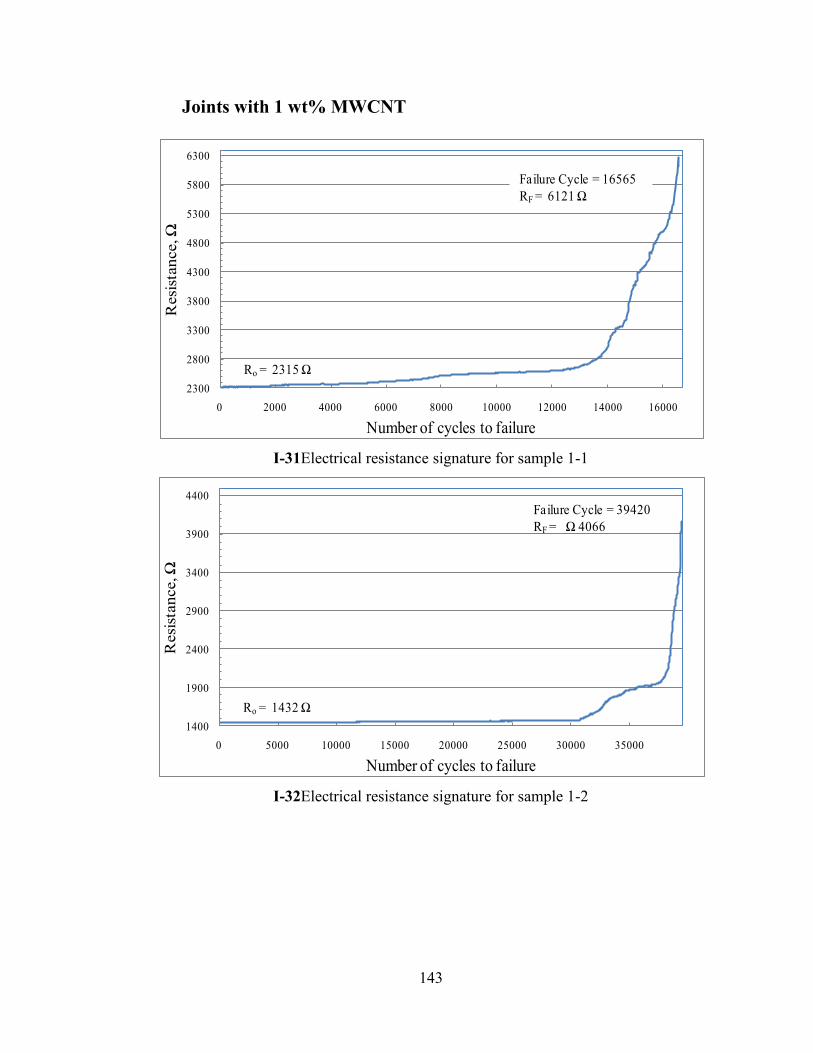
143
Joints with 1 wt% MWCNT
I-31Electrical resistance signature for sample 1-1
I-32Electrical resistance signature for sample 1-2
2300
2800
3300
3800
4300
4800
5300
5800
6300
0 2000 4000 6000 8000 10000 12000 14000 16000
Resi
stan
ce, Ω
Number of cycles to failure
Ro = 2315 Ω
Failure Cycle = 16565
RF = 6121 Ω
1400
1900
2400
2900
3400
3900
4400
0 5000 10000 15000 20000 25000 30000 35000
Resi
stan
ce, Ω
Number of cycles to failure
Ro = 1432 Ω
Failure Cycle = 39420
RF = Ω 4066
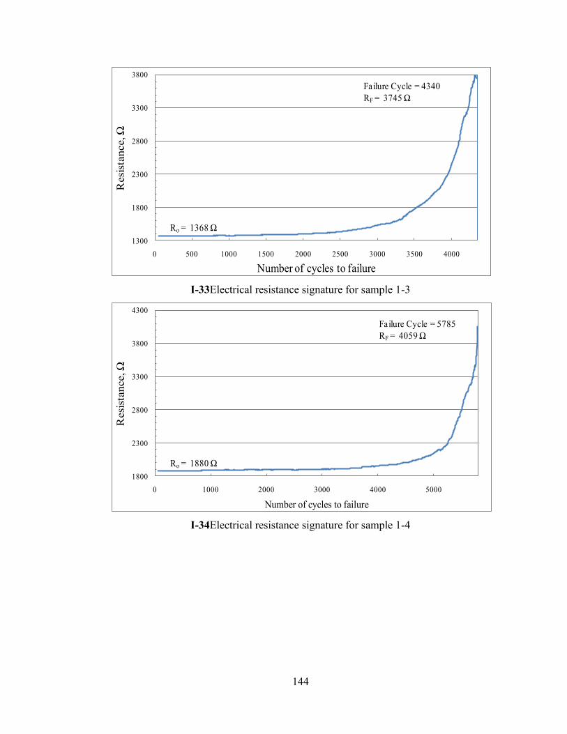
144
I-33Electrical resistance signature for sample 1-3
I-34Electrical resistance signature for sample 1-4
1300
1800
2300
2800
3300
3800
0 500 1000 1500 2000 2500 3000 3500 4000
Resi
stance, Ω
Number of cycles to failure
Ro = 1368 Ω
Failure Cycle = 4340
RF = 3745 Ω
1800
2300
2800
3300
3800
4300
0 1000 2000 3000 4000 5000
Resi
stance, Ω
Number of cycles to failure
Ro = 1880 Ω
Failure Cycle = 5785
RF = 4059 Ω

145
I-35Electrical resistance signature for sample 1-5
I-36Electrical resistance signature for sample 1-6
700
900
1100
1300
1500
1700
1900
2100
0 1000 2000 3000 4000 5000 6000
Resi
stance, Ω
Number of cycles to failure
Ro =746 Ω
Failure Cycle = 6610
RF = 1991 Ω
1800
2300
2800
3300
3800
4300
0 2000 4000 6000 8000 10000
Resi
stan
ce, Ω
Number of cycles to failure
Ro = 1848 Ω
Failure Cycle = 10580
RF = 3933 Ω
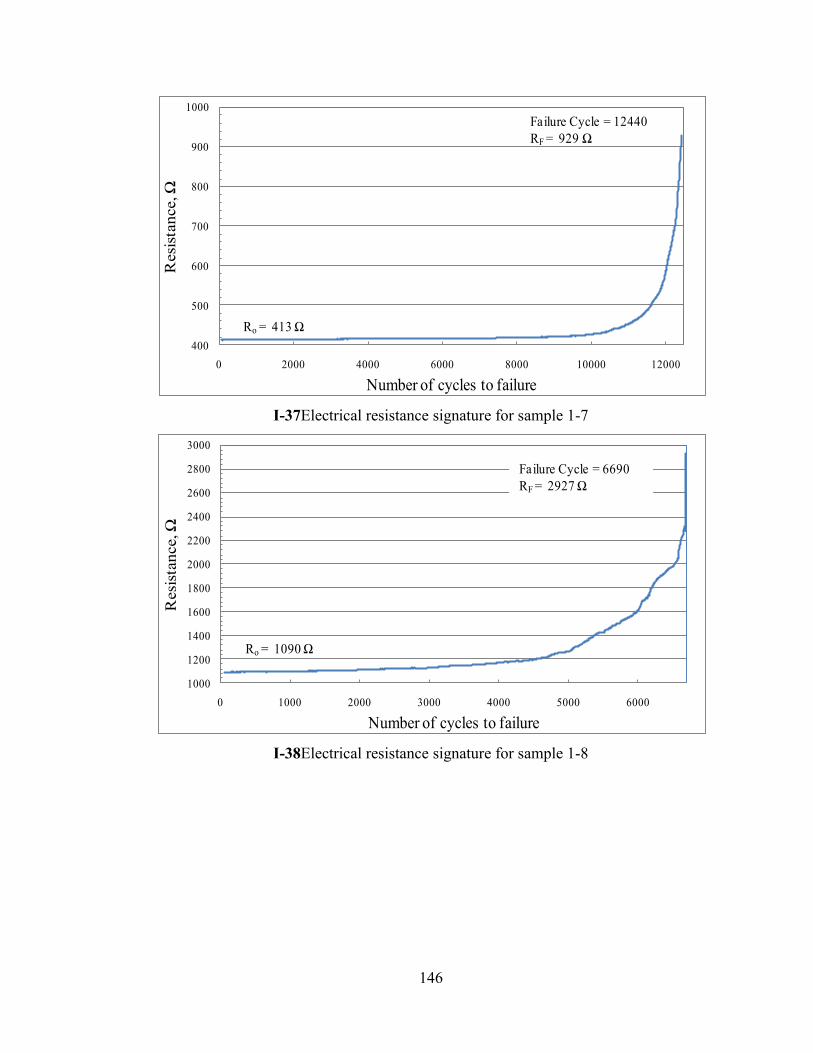
146
I-37Electrical resistance signature for sample 1-7
I-38Electrical resistance signature for sample 1-8
400
500
600
700
800
900
1000
0 2000 4000 6000 8000 10000 12000
Resi
stan
ce, Ω
Number of cycles to failure
Ro = 413 Ω
Failure Cycle = 12440
RF = 929 Ω
1000
1200
1400
1600
1800
2000
2200
2400
2600
2800
3000
0 1000 2000 3000 4000 5000 6000
Resi
stance, Ω
Number of cycles to failure
Ro = 1090 Ω
Failure Cycle = 6690
RF = 2927 Ω
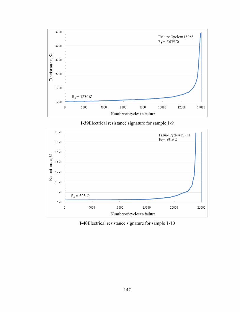
147
I-39Electrical resistance signature for sample 1-9
I-40Electrical resistance signature for sample 1-10
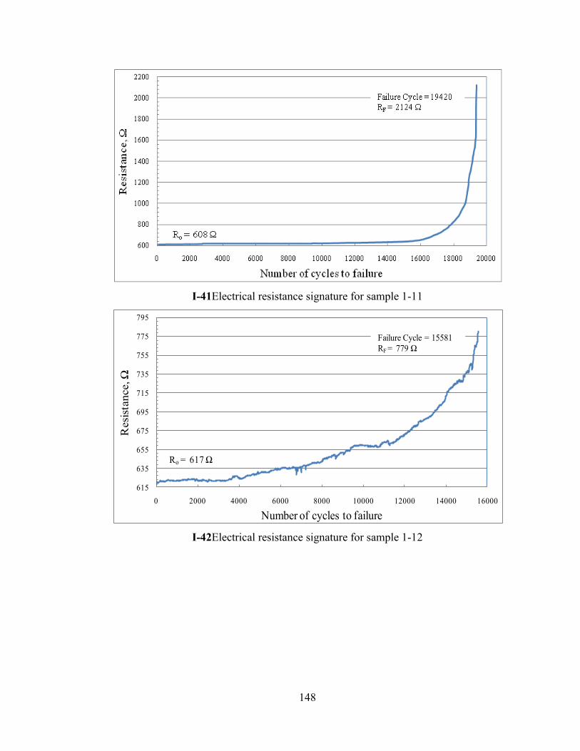
148
I-41Electrical resistance signature for sample 1-11
I-42Electrical resistance signature for sample 1-12
615
635
655
675
695
715
735
755
775
795
0 2000 4000 6000 8000 10000 12000 14000 16000
Resi
stan
ce, Ω
Number of cycles to failure
Ro = 617 Ω
Failure Cycle = 15581
RF = 779 Ω

149
I-43Electrical resistance signature for sample 1-13
I-44Electrical resistance signature for sample 1-14
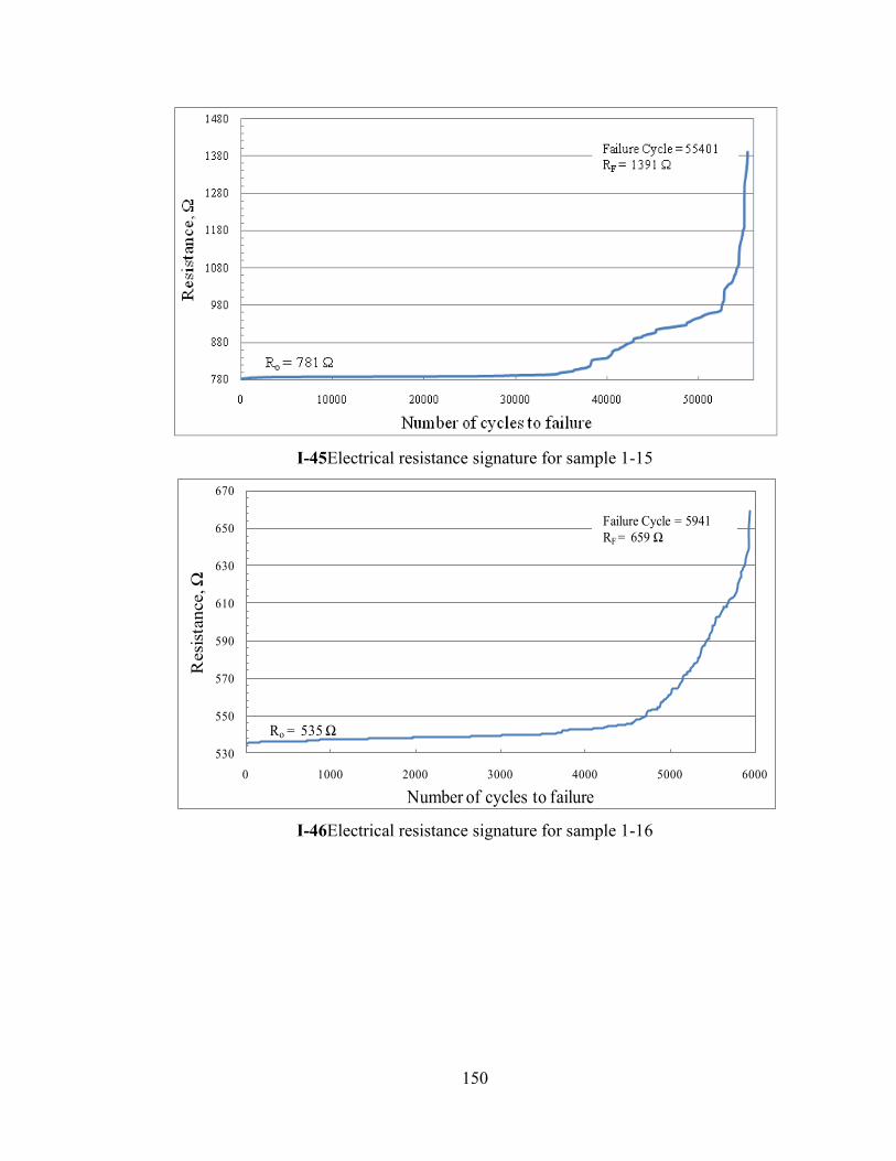
150
I-45Electrical resistance signature for sample 1-15
I-46Electrical resistance signature for sample 1-16
530
550
570
590
610
630
650
670
0 1000 2000 3000 4000 5000 6000
Resi
stan
ce, Ω
Number of cycles to failure
Ro = 535 Ω
Failure Cycle = 5941
RF = 659 Ω
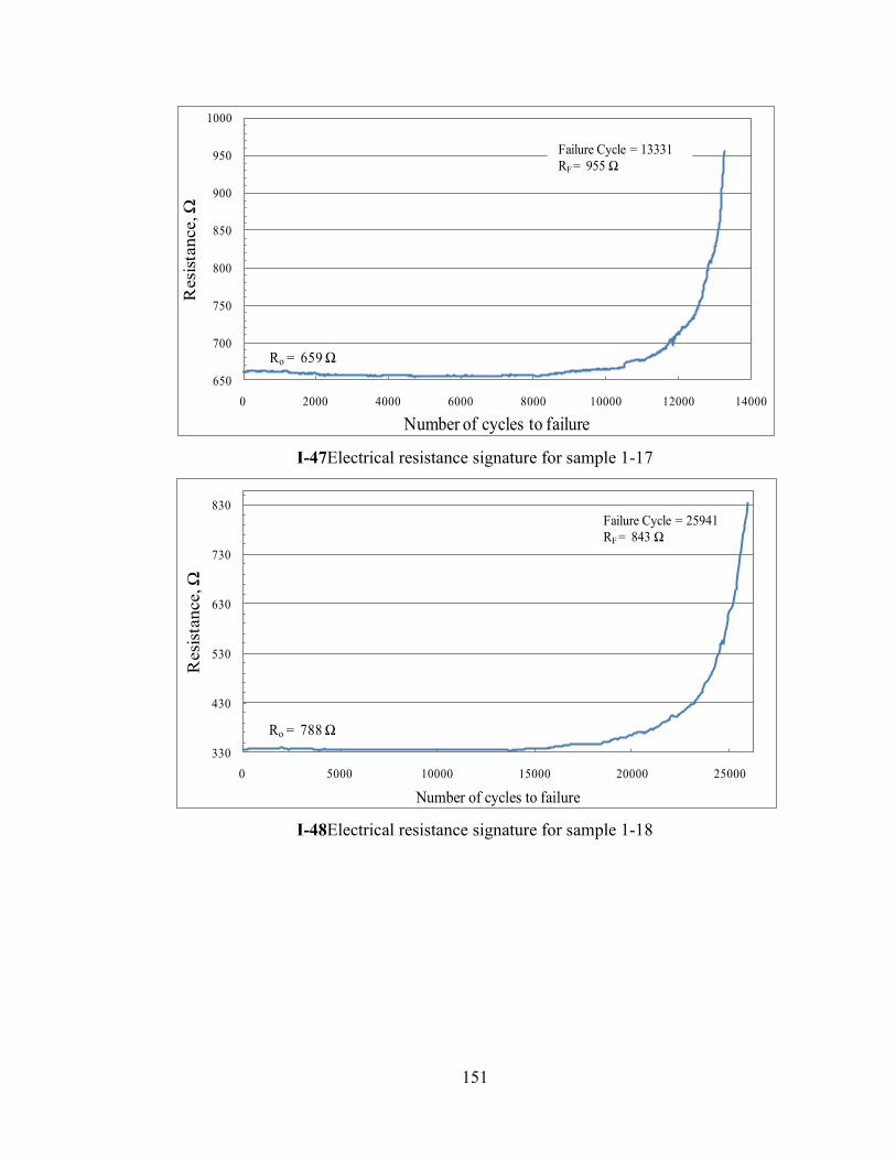
151
I-47Electrical resistance signature for sample 1-17
I-48Electrical resistance signature for sample 1-18
650
700
750
800
850
900
950
1000
0 2000 4000 6000 8000 10000 12000 14000
Resi
stan
ce, Ω
Number of cycles to failure
Ro = 659 Ω
Failure Cycle = 13331
RF = 955 Ω
330
430
530
630
730
830
0 5000 10000 15000 20000 25000
Resi
stan
ce, Ω
Number of cycles to failure
Ro = 788 Ω
Failure Cycle = 25941
RF = 843 Ω

152
I-49Electrical resistance signature for sample 1-19
I-50Electrical resistance signature for sample 1-20
160
180
200
220
240
260
280
300
320
0 2000 4000 6000 8000 10000 12000 14000
Resi
stan
ce, Ω
Number of cycles to failure
Ro = 169 Ω
Failure Cycle = 13941
RF = 310 Ω
87
97
107
117
127
137
147
157
167
177
0 2000 4000 6000 8000 10000 12000
Resi
stance, Ω
Number of cycles to failure
Ro = 87 Ω
Failure Cycle = 12741
RF = 175 Ω
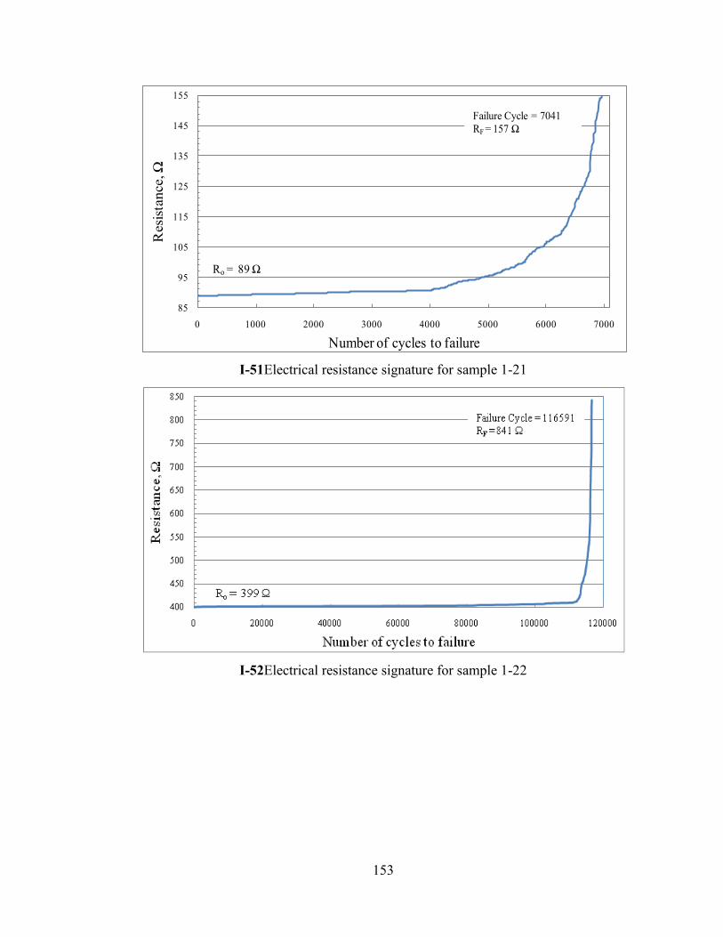
153
I-51Electrical resistance signature for sample 1-21
I-52Electrical resistance signature for sample 1-22
85
95
105
115
125
135
145
155
0 1000 2000 3000 4000 5000 6000 7000
Resi
stance, Ω
Number of cycles to failure
Ro = 89 Ω
Failure Cycle = 7041
RF = 157 Ω

154
I-53Electrical resistance signature for sample 1-23
I-54Electrical resistance signature for sample 1-24
270
370
470
570
670
770
870
0 2000 4000 6000 8000 10000 12000 14000
Resi
stance, Ω
Number of cycles to failure
Ro = 276Ω
Failure Cycle = 14441
RF = 902 Ω
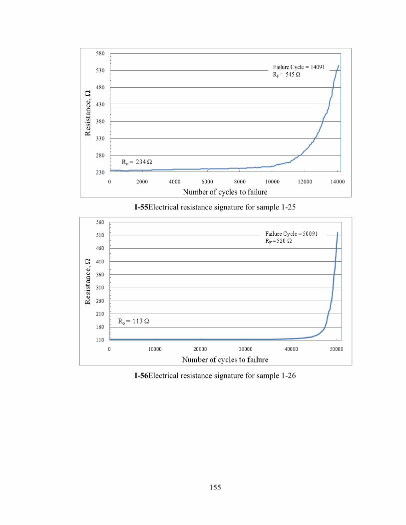
155
I-55Electrical resistance signature for sample 1-25
I-56Electrical resistance signature for sample 1-26
230
280
330
380
430
480
530
580
0 2000 4000 6000 8000 10000 12000 14000
Resi
stan
ce, Ω
Number of cycles to failure
Ro = 234 Ω
Failure Cycle = 14091
RF = 545 Ω
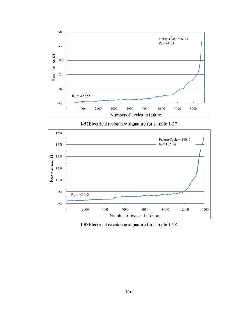
156
I-57Electrical resistance signature for sample 1-27
I-58Electrical resistance signature for sample 1-28
430
480
530
580
630
680
0 1000 2000 3000 4000 5000 6000 7000 8000
Resi
stan
ce, Ω
Number of cycles to failure
Ro = 432 Ω
Failure Cycle = 8525
RF = 644 Ω
650
850
1050
1250
1450
1650
1850
0 2000 4000 6000 8000 10000 12000 14000
Resi
stan
ce, Ω
Number of cycles to failure
Ro = 690 Ω
Failure Cycle = 14000
RF = 1822 Ω
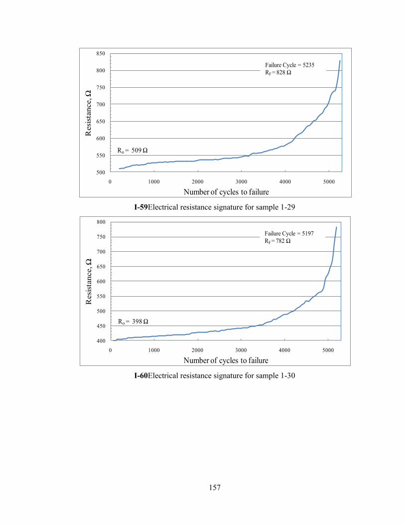
157
I-59Electrical resistance signature for sample 1-29
I-60Electrical resistance signature for sample 1-30
500
550
600
650
700
750
800
850
0 1000 2000 3000 4000 5000
Resi
stan
ce, Ω
Number of cycles to failure
Ro = 509 Ω
Failure Cycle = 5235
RF = 828 Ω
400
450
500
550
600
650
700
750
800
0 1000 2000 3000 4000 5000
Resi
stan
ce, Ω
Number of cycles to failure
Ro = 398 Ω
Failure Cycle = 5197
RF = 782 Ω
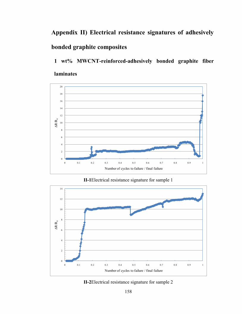
158
Appendix II) Electrical resistance signatures of adhesively
bonded graphite composites
1 wt% MWCNT-reinforced-adhesively bonded graphite fiber
laminates
II-1Electrical resistance signature for sample 1
II-2Electrical resistance signature for sample 2
0
2
4
6
8
10
12
14
16
18
20
0 0.1 0.2 0.3 0.4 0.5 0.6 0.7 0.8 0.9 1
∆R
/Ro
Number of cycles to failure / final failure
0
2
4
6
8
10
12
14
0 0.1 0.2 0.3 0.4 0.5 0.6 0.7 0.8 0.9 1
∆R
/Ro
Number of cycles to failure / final failure

159
II-3Electrical resistance signature for sample 3
II-4Electrical resistance signature for sample 4
0
10
20
30
40
50
60
70
80
90
0 0.1 0.2 0.3 0.4 0.5 0.6 0.7 0.8 0.9 1
∆R
/Ro
Number of cycles to failure / final failure
0
1
2
3
4
5
6
7
0 0.1 0.2 0.3 0.4 0.5 0.6 0.7 0.8 0.9 1
∆R
/Ro
Number of cycles to failure / final failure