In-Flight Stability Analysis of the X-48B Aircraft · American Institute of Aeronautics and...

American Institute of Aeronautics and Astronautics

092407

1

In-Flight Stability Analysis of the X-48B Aircraft

Christopher D. Regan * NASA Dryden Flight Research Center, Edwards, California, 93505

This report presents the system description, methods, and sample results of the in-flight stability analysis for the X-48B, Blended Wing Body Low-Speed Vehicle. The X-48B vehicle is a dynamically scaled, remotely piloted vehicle developed to investigate the low-speed control characteristics of a full-scale blended wing body. Initial envelope clearance was conducted by analyzing the stability margin estimation resulting from the rigid aircraft response during flight and comparing it to simulation data. Short duration multisine signals were commanded onboard to simultaneously excite the primary rigid body axes. In-flight stability analysis has proven to be a critical component of the initial envelope expansion.

Nomenclature BWB = Blended Wing Body d = excitation signal C1 = flight controller C2 = control surface allocation portion of the flight controller CG = center of gravity deg = degree DFRC = Dryden Flight Research Center DFT = discreet Fourier transform M = number of multisine excitation components P = aircraft plant PF = peak factor Pk = relative power of component, k, of the multisine excitation k = component of multisine excitation j = channel of excitation application r = outer-loop controller commands RTSM = real-time stability margin t = time u = actuator commands VMS = vehicle management system x = controller command after excitation y = controller command prior to excitation !k = frequency of component, k, of the multisine excitation !k = phase of component, k, of the multisine excitation

I. Introduction HE X-48B vehicle (Fig. 1) is an 8.5-percent dynamically scaled Blended Wing Body (BWB) constructed for The Boeing Company (Boeing Phantom Works, Huntington Beach, California) by Cranfield Aerospace Ltd.

(Bedford, United Kingdom). The first flight of the X-48B vehicle occurred on July 20, 2007, at the NASA Dryden Flight Research Center (DFRC, Edwards, California). This scaled, remotely piloted vehicle was developed to investigate the low-speed stability and control characteristics of a full-scale BWB. The X-48B aircraft has a wingspan of 20.4 ft, maximum weight of 525 lb, and fuel-carrying capacity of approximately 13 gal. The aircraft uses three modified JetCat USA (Paso Robles, California) P200 turbojet engines, each capable of 54 lb of installed thrust. The aircraft takes off and lands conventionally with fixed tricycle-type landing gear. Two leading-edge slat * Aerospace Engineer, Controls and Dynamics Branch, P.O. Box 273/MS:4840D, AIAA Member.

T

https://ntrs.nasa.gov/search.jsp?R=20080034515 2018-07-26T03:34:19+00:00Z


092407

2

configurations, extended and retracted, are available and can be interchanged between flights. The flight duration during initial flight tests has been 30-35 min per flight, only a fraction of which is available for flight test maneuvers and excitations.

Figure 1. The X-48B aircraft.

The general approach for analyzing stability during flight has undergone an evolutionary maturation process. Excitations provide the basis for estimation of open-loop frequency responses and transfer functions at a particular flight condition. The estimated transfer functions are then used for the stability margin analysis. Measuring, analyzing, and reporting stability margins, and comparing simulation data to flight data, provide an abundance of useful information for rapid envelope expansion. This report presents the implementation of in-flight stability analysis that represents the latest stage of an evolutionary development. The short flight duration of the X-48B vehicle has driven the development toward a particular class of excitations that provide short-duration, multiaxis capability.

Early examples of the in-flight stability analysis techniques were developed at the NASA DFRC for the Grumman X-29A vehicle.1,2 These examples involved hand-flown frequency sweeps and in-flight stability analysis. Flight-testing of the McDonnell Douglas X-36 vehicle incorporated frequency sweep excitations into an automated system.3 More recently, flight-testing of the X-43A vehicle (ATK GASL, Tullahoma, Tennessee) and the McDonnell Douglas (now Boeing) NF-15B Intelligent Flight Control Systems aircraft used automated injection of multisine excitations during flight to simultaneously characterize the stability of multiple axes with postflight analysis.4,5 Flight-testing of the X-48B aircraft uses the foundations of in-flight analysis developed for the X-29A vehicle with the type of automated, short-duration excitations developed for use on the X-43A vehicle.

II. System Description The vehicle management system (VMS) that operated on board the flight control computer was developed by

The Boeing Company. The VMS partially consists of a dynamic inversion–based inner-loop control augmentation system. Multiple options for internal excitation have been incorporated into the VMS, including multiple injection points and waveforms. This report focuses on excitation at a single injection point with a particular type of excitation signal expressly incorporated into the VMS for in-flight stability analysis.

Figure 2 shows the location of the excitation signal in relation to the closed-loop system. The injection point of the excitation signal, d, is just prior to control surface allocation, C2 , subsystem. This location minimizes controller dimensionality, reducing it to three channels. The excitation corresponds to the three principle axes related to roll,


092407

3

pitch, and yaw rate commands. This location also reduces the potential impact of additional feedback paths from the plant, P, from influencing the open-loop transfer function.

The vehicle’s open-loop transfer function, C1PC2 , can be estimated from closed-loop time histories.1 Equation (1) shows the initial step in forming the transfer function from time history signals. Commands associated with the outer loops, r, including pilot commands, are procedurally minimized during excitation maneuvers and are ignored for this analysis. A number of possible options are available for estimating the open-loop transfer function. Equation (2) shows the simple transfer function form using the controller command signals, x and y. Equation (3) is the preferred formation using the controller command, y, and the excitation signal, d. This formation eliminates the impact of noise correlation between the x and y signals in the transfer function estimation.6

Figure 2 . Simplified representation of the closed-loop system.

y = C1r ! C1PC2x (1)

C1PC2 =!y

x (2)

C1PC2 =

!yd

1+yd

(3)

III. Excitation Description The excitations signals used for the in-flight stability margin estimation of the X-48B vehicle are intended to

operate across the flight envelope. Because of the short flight duration, the use of short-duration and content rich excitations is preferred. The excitations use a simple form of the multisine signal shown in Eq. (4). In general, multisines allow for freedom in selection of the frequency components, !k , and the relative power of each frequency component, Pk . To guarantee that the signals, d j , are mutually orthogonal, the frequency components are chosen as components of a harmonic sequence. The orthogonal nature of the excitation signals allows for simultaneous excitation of each channel, which further reduces the time required for excitations.

d j =Pk

2k=1

M

! cos "kt + #k( ) (4)

For the aircraft to maintain flight near its initial equilibrium, or trim point, the excitation peak factor (PF) should be minimized as shown in Eq. (5). Minimization of the peak factor also enables maximization of excitation power for a given dynamic excursion from the trim condition. Peak factor is minimized through selection of the phase angle, !k , of each frequency component, !k . Schroeder found that selection of phase angles following a quadratic function of frequency would result in a consistently low peak factor.7 Morelli extended the selection of phase angles


092407

4

and further reduced the peak factor by implementing a simplex optimization algorithm that seeks to minimize the peak factor through optimal phase angle selection.5

PF d j( ) =max d j( ) !min d j( )

2rms d j( ) (5)

For the X-48B vehicle, two excitations, following the procedure laid out by Morelli, have been developed for the

purposes of transfer function estimation. Table 1 summarizes these excitations. Both excitations target a frequency band between 1 and 75 rad/s and have flat spectra in each channel. Multisine 1 was developed with tight frequency spacing and minimal duration. Because of concerns related to nonlinearities in the actuator responses and low-frequency response, an alternate multisine was created and incorporated in the VMS. Multisine 2 was developed with one-third the frequency components, which increased the frequency separation. Multisine 2 is also longer in duration, consisting of five repetitions of the lowest component frequency, as opposed to three repetitions for multisine 1. During nonlinear and piloted simulations it was determined that for adequate excitation in the roll and pitch axes, the yaw axis excitation amplitude resulted in excessive control surface commands. A scale factor was placed on the yaw channel excitation to reduce the amplitude of the yaw excitation, thereby reducing the control surface movement. Figure 3 shows a portion of the yaw channel excitation time history and aircraft response.

Figure 3. Time history of the first 10 s of the yaw channel excitation and yaw response normalized by the excitation magnitude.


092407

5

Table 1. Multisine excitation parameters.

Multisine 1 Multisine 2 Minimum frequency, rad/s 1.0 1.0 Maximum frequency, rad/s 74.0 75.0 Frequency component separation rad/s 0.3 1.0 Lowest frequency repeats 3.0 5.0 Total duration, s 19.0 31.0 Power spectrum Flat Flat

The component phases were shifted for both multisines to yield near zero initial and final values.5 This shift

eliminates the frequency leakage effect, which deemphasizes the importance of windowing, and does not affect the excitation peak factor. Transformation from time domain to frequency domain was initially performed using a discrete Fourier transform (DFT). This transformation provided good results for tightly spaced frequency components, as in multisine 1. With the introduction of multisine 2, a chirp-z transformation was implemented and became the preferred transformation for use with both multisines. The chirp-z transform allows for selection of the particular frequency band included in the transformation, which provides a good capabilities match to the definition of the multisine.

Figure 4 shows a comparison between the DFT and chirp-z transform, as computed using data from an in-flight excitation with multisine 1. There is a marked difference in the coherence level. This difference is attributed mostly to smoothing effects associated with the DFT computation performed at frequencies that are not explicitly contained in the excitation. The comparison also shows that the DFT contains frequencies that extend beyond the excited frequency range, and shows that the chirp-z transform is typically smoother. The smoother response exhibited by the chirp-z transform removes some of the sensitivity associated with determining the gain and phase crossover frequencies. The decreased sensitivity improves repeatability, thereby allowing for easier interpretation of comparisons between flight and simulation data.

Figure 4. Bode plot comparison of discrete Fourier transform with chirp-z transform in the roll axis.

IV. In-Flight Operations The X-48B aircraft is flown remotely from a purpose-built ground control station (GCS). The GCS contains a

pilot station, flight test engineer station, and range safety officer console. In addition, a GCS operator station and real-time stability margin (RTSM) operator station are located next to the GCS.


092407

6

The RTSM terminal records a subset of the telemetry signal received from the aircraft during each execution of the onboard excitation system. Excitations are selected by the flight test engineer, confirmed by the test conductor, and executed by the flight test engineer. Upon completion of the excitation, the RTSM operator begins an evaluation of the maneuver. The RTSM terminal software has been developed with an emphasis on comparison with precomputed simulation results in addition to the estimated in-flight stability margin. Comparison with simulation is performed using nonlinear simulation–based time-history data of the same excitation at approximately the same flight conditions. The comparison is performed in the frequency domain by means of overplotting flight and simulation data on Bode plots.

Stability margins, in terms of gain and phase margins, are evaluated following each RTSM excitation. The system is treated as nine single-input, single-output (SISO) transfer functions, incorporating all possible combinations of the three inputs and three outputs. Treating the system as nine SISO transfer functions is possible, because the excitation signal channels are mutually orthogonal and the resulting transfer function loops are decorrelated. It was determined that the insight provided by evaluating each SISO system independently on Bode plots was worth the extra time associated with the additional analysis. Stability analysis can be completed in approximately 45 s, from initiation of the excitation to completed stability evaluation.

V. Flight Test Results This section summarizes the results obtained during the initial flight-testing of the X-48B aircraft in the slats-

extended configuration. As of this writing, 11 flights have been conducted. During these flights only the excitation labeled multisine 1 has been flown. The concerns motivating the development of multisine 2 have not been seen in the flight data.

Flight envelope expansion has been conducted in a buildup fashion. The vehicle has a limited altitude envelope, and the predicted stability of the vehicle is insensitive within the altitude range of interest. For this reason, envelope expansion has focused on airspeed, center of gravity (CG) location, and slat configuration. Slat configuration, extended or retracted, is treated as a major configuration change; envelope clearance for each configuration is treated separately. The buildup approach is to clear an airspeed range in the center of the total range for a mid-CG configuration. The CG configuration is then altered between flights by moving ballast weight. The CG location clearance follows a mid, forward, aft sequence. Each flight condition is cleared by performing an integrated test block that consists of small amplitude piloted maneuvers and excitations for stability estimation.

During the first 11 flights of the X-48B aircraft, the RTSM system was used to clear 10 flight conditions. The slats-extended configuration with mid, forward, and aft CG was flown. Tables 2 through 5 compare predicted stability margins, from nonlinear simulation, with flight estimated stability margins. Thus far, flight results have matched the nonlinear simulation results quite well, providing confidence in the simulation and aerodynamic modeling.


092407

7

Table 2. Comparison of predicted stability margins with flight estimated stability margins for flight 3; mid center of gravity, slats extended.

Predicted stability margins Flight-based stability margins Altitude,

ft Airspeed,

knots Axis Gain margin, dB

at rad/s Phase margin,

deg at rad/s Gain margin, dB


deg at rad/s 7242 57.0 Roll 19.9 at 22.3 Infinite 16.3 at 21.7 Infinite 7242 57.0 Pitch 12.0 at 23.0 65.8 at 6.7 15.0 at 28.7 64.1 at 7.4 7242 57.0 Yaw 16.6 at 15.6 71.2 at 2.9 15.2 at 19.2 69.4 at 3.0 7234 62.9 Roll 21.9 at 23.5 Infinite 16.6 at 23.0 Infinite 7234 62.9 Pitch 13.7 at 27.0 71.7 at 5.9 14.9 at 29.0 75.4 at 7.4 7234 62.9 Yaw 16.1 at 16.7 67.3 at 3.9 15.0 at 20.9 70.4 at 3.5 7243 78.0 Roll 16.4 at 24.4 Infinite 14.2 at 26.2 Infinite 7243 78.0 Pitch 12.6 at 28.8 83.2 at 5.9 14.5 at 30.9 92.0 at 7.6 7243 78.0 Yaw 14.2 at 21.4 71.1 at 4.9 15.9 at 27.2 74.2 at 3.6 Table 3. Comparison of predicted stability margins with flight estimated stability margins for flight 4; forward center of gravity, slats extended.


ft Airspeed,





deg at rad/s 7226 49.7 Roll 17.1 at 22.1 120.0 at 5.7 15.5 at 21.6 81.4 at 2.7 7226 49.7 Pitch 10.6 at 22.6 54.8 at 7.7 16.2 at 29.0 51.9 at 7.9 7226 49.7 Yaw 20.5 at 16.4 63.2 at 2.2 18.8 at 18.6 42.3 at 1.8 7311 65.6 Roll 20.3 at 23.9 Infinite 18.7 at 24.4 Infinite 7311 65.6 Pitch 14.0 at 27.2 76.1 at 2.9 15.4 at 29.0 83.1 at 7.1 7311 65.6 Yaw 16.2 at 17.3 68.7 at 4.1 15.0 at 22.0 62.5 at 3.7 7320 75.9 Roll 18.0 at 24.6 Infinite 16.4 at 26.0 Infinite 7320 75.9 Pitch 12.1 at 28.9 87.0 at 3.0 15.7 at 30.7 89.9 at 7.5 7320 75.9 Yaw 14.4 at 20.0 70.9 at 4.9 15.9 at 26.8 71.0 at 3.9 Table 4. Comparison of predicted stability margins with flight estimated stability margins for flight 6; forward center of gravity, slats extended. Predicted stability margins Flight-based stability margins Altitude,

ft Airspeed,





deg at rad/s 3970 53.6 Roll 20.5 at 22.5 Infinite 18.4 at 21.8 Infinite 3970 53.6 Pitch 12.4 at 23.2 64.0 at 7.2 17.0 at 30.4 58.7 at 7.7 3970 53.6 Yaw 17.5 at 16.3 73.5 at 2.8 16.8 at 19.1 49.4 at 2.3


092407

8

Table 5. Comparison of predicted stability margins with flight estimated stability margins for flight 9; aft center of gravity, slats extended.


ft Airspeed,





deg at rad/s 6910 53.6 Roll 13.6 at 18.9 114.0 at 5.0 12.9 at 18.5 102.0 at 6.3 6910 53.6 Pitch 10.4 at 18.6 49.7 at 6.4 11.9 at 21.0 54.7 at 7.4 6910 53.6 Yaw 14.5 at 16.2 62.6 at 3.1 13.9 at 16.3 56.1 at 3.1 5450 65.4 Roll 14.9 at 22.4 123.0 at 5.2 14.2 at 22.1 Infinite 5450 65.4 Pitch 11.5 at 21.6 67.0 at 6.9 15.1 at 27.1 69.1 at 7.4 5450 65.4 Yaw 14.4 at 18.1 62.9 at 4.1 14.6 at 19.3 63.1 at 3.6 6950 76.1 Roll 11.1 at 24.0 96.6 at 7.3 10.7 at 23.7 106.0 at 6.5 6950 76.1 Pitch 12.2 at 26.4 88.1 at 6.1 13.0 at 29.0 74.0 at 8.2 6950 76.1 Yaw 14.7 at 24.8 67.6 at 4.3 15.1 at 23.6 66.8 at 3.9

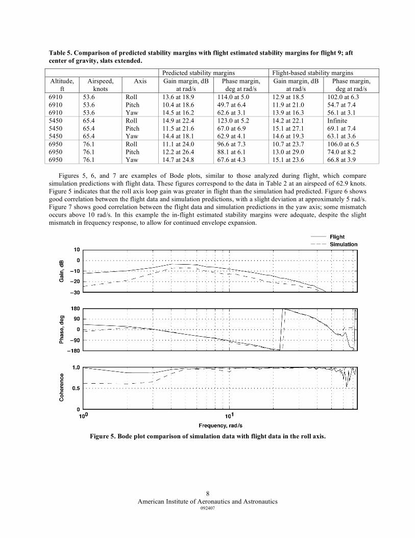
Figures 5, 6, and 7 are examples of Bode plots, similar to those analyzed during flight, which compare

simulation predictions with flight data. These figures correspond to the data in Table 2 at an airspeed of 62.9 knots. Figure 5 indicates that the roll axis loop gain was greater in flight than the simulation had predicted. Figure 6 shows good correlation between the flight data and simulation predictions, with a slight deviation at approximately 5 rad/s. Figure 7 shows good correlation between the flight data and simulation predictions in the yaw axis; some mismatch occurs above 10 rad/s. In this example the in-flight estimated stability margins were adequate, despite the slight mismatch in frequency response, to allow for continued envelope expansion.

Figure 5. Bode plot comparison of simulation data with flight data in the roll axis.


092407

9

Figure 6. Bode plot comparison of simulation data with flight data in the pitch axis.

Figure 7. Bode plot comparison of simulation data with flight data in the yaw axis.


092407

10

VI. Conclusion An efficient in-flight stability margin estimation method was developed for flight-testing and initial envelope

clearance of the X-48B vehicle. The limited flight duration of the vehicle motivated the use of multisine excitation signals to simultaneously excite all three axes. The chirp-z transformation was found to be a good fit with this type of excitation signal. The approach that was implemented relies on simulation data for comparison and clearance, and all nine potential transfer functions were found to provide beneficial information for the comparison. Analysis thus far indicates good frequency domain matches between flight data and simulation predictions. The quality of matches between the flight data and simulation predictions and the stability analysis conducted thus far have provided confidence in the simulation modeling, particularly in aerodynamics modeling. Future efforts at the NASA Dryden Flight Research Center to advance the application of in-flight stability are focused on incorporation of true real-time transfer function estimation and multiple-input, multiple-output analysis.

References 1Bosworth, J.T., and West, J.C., “Real-Time Open-Loop Frequency Response Analysis of Flight Test Data,” AIAA 86-9738,

1986. 2Gera, J., and Bosworth, J.T., “Dynamic Stability and Handling Qualities Tests on a Highly Augmented, Statically Unstable

Airplane,” NASA TM-88297, 1987. 3Balough, D.L., “Determination of X-36 Stability Margins Using Real-Time Frequency Response Techniques,” AIAA-98-

4154, 1998. 4Baumann, E., “Tailored Excitation for Frequency Response Measurement Applied to the X-43A Flight Vehicle,” AIAA-

2006-638, 2006. 5Morelli, E.A., “Multiple Input Design for Real-Time Parameter Estimation in the Frequency Domain,” Paper REG-360, 13th

IFAC Symposium on System Identification, Rotterdam, The Netherlands, August 2003. 6Tischler, M.B., and Remple, R.K. Aircraft and Rotorcraft System Identification: Engineering Methods with Flight Test

Examples, AIAA Education Series, AIAA, Inc., Reston, VA, 2006.

7Schroeder, M., “Synthesis of Low-Peak-Factor Signals and Binary Sequences with Low Autocorrelation,” IEEE Transactions On Information Theory, Vol. 16, No. 1, Jan. 1970, pp. 85–89.

In-Flight Stability Analysis of the X-48B Aircraft · American Institute of Aeronautics and...

Documents

Transcript of In-Flight Stability Analysis of the X-48B Aircraft · American Institute of Aeronautics and...