In Copyright - Non-Commercial Use Permitted Rights ...48877/...Finally, a novel approach to the...
129
Research Collection Doctoral Thesis Radiation dosimetry of clinical proton beams Author(s): Gomà Estadella, Carles Publication Date: 2016 Permanent Link: https://doi.org/10.3929/ethz-a-010618824 Rights / License: In Copyright - Non-Commercial Use Permitted This page was generated automatically upon download from the ETH Zurich Research Collection . For more information please consult the Terms of use . ETH Library
-
Upload
vuongtuong -
Category
Documents
-
view
214 -
download
0
Transcript of In Copyright - Non-Commercial Use Permitted Rights ...48877/...Finally, a novel approach to the...

Research Collection
Doctoral Thesis
Radiation dosimetry of clinical proton beams
Author(s): Gomà Estadella, Carles
Publication Date: 2016
Permanent Link: https://doi.org/10.3929/ethz-a-010618824
Rights / License: In Copyright - Non-Commercial Use Permitted
This page was generated automatically upon download from the ETH Zurich Research Collection. For moreinformation please consult the Terms of use.
ETH Library

DISS. ETH NO. 23198
Radiation dosimetry ofclinical proton beams
A thesis submitted to attain the degree ofDOCTOR OF SCIENCES of ETH ZURICH
(Dr. sc. ETH Zurich)
presented byCarles Gomà Estadella
Lic. Physics, University of Barcelonaborn on 19.07.1983
citizen of Spain
accepted on the recommendation ofProf. Dr. Antony Lomax
Prof. Dr. Günther DissertoriDr. Sairos Safai
Dr. Josep Sempau
2016
This thesis has been officially supervised by
Prof. Dr. Antony LomaxETH Zurich, Department of PhysicsPaul Scherrer Institute, Center for Proton Therapy
and co-supervised by
Dr. Josep SempauUniversitat Politècnica de Catalunya, Institut de Tècniques Energètiques
and
Dr. Sairos SafaiPaul Scherrer Institute, Center for Proton Therapy

“I can think, I can wait, I can fast”
Siddhartha


Abstract
The aim of this thesis is to improve the accuracy and reduce the uncertaintyin the radiation dosimetry of radiotherapy proton pencil beams. Specialemphasis is put on the absolute determination of the absorbed dose to water.
To that aim, Monte Carlo simulation techniques were used to calculatecornerstone quantities for the relative and reference dosimetry of proton pen-cil beams, namely water/medium stopping-power ratios and beam qualitycorrection factors. Monte Carlo calculations were validated with experi-mental data obtained with ionization chamber and Faraday cup dosimetry.Finally, a novel approach to the reference dosimetry of proton pencil beamsbased on the concept of ‘dose-area product’ was described and its feasibilityassessed.
The Monte Carlo calculation of water/medium stopping-power ratios re-vealed that the most suitable detection materials for the relative dosimetryof proton pencil beams in water are air and radiochromic film active layer.Lithium fluoride and silicon may also be used for the measurement of lateraldose profiles and field-specific dose distributions in water; whereas the useof gadolinium oxysulfide should be limited to relative dose measurementsin air. Concerning reference dosimetry, it appears that the largest sourceof uncertainty in the water/air stopping-power ratios arises from the uncer-tainty of the mean excitation energy of water—where an increase of 3 eVresults in a decrease of approximately 0.6% in the water/air stopping-powerratios.
The Monte Carlo calculation of beam quality correction factors yieldedresults which agree within 2.3% with the values tabulated in IAEA TRS-398 Code of Practice, and within 1% with published experimental valuesobtained with water calorimetry. These results also point at ionizationchamber perturbation correction factors in proton beams that may differsignificantly from unity.
Reference dosimetry based on IAEA TRS-398 was compared to Faradaycup dosimetry. These two independent dosimetry techniques were found toagree within approximately 3% when using IAEA TRS-398 beam qualitycorrection factors, and within approximately 1.5% when using the MonteCarlo beam quality correction factors calculated in this work. This compar-ison also pointed at a systematic error in the determination of the absorbed
v

vi
dose to water, especially relevant for low-energy proton beams, when usingcylindrical ionization chambers together with IAEA TRS-398 reference con-ditions for monoenergetic proton beams. This error, which arises from therecommendation of positioning the reference point of cylindrical chambersat the reference depth, could be corrected by (i) positioning the effectivepoint of measurement at the reference depth or (ii) including a correctionfor dose gradient effects in the beam quality correction factors.
Finally, a novel approach to the reference dosimetry of proton pencilbeams was described. This approach, based on the determination of thedose-area product of a single proton pencil beam, was shown to be feasibleand equivalent to the standard approach based on the determination of theabsorbed dose to water at the centre of a uniform broad field.

Zusammenfassung
Das Ziel dieser Doktorarbeit ist es, sowohl die Richtigkeit als auch die Prä-zision in der Dosimetrie von therapeutischen Protonen-Nadelstrahlen zu er-höhen. Der Fokus liegt dabei auf der absoluten Bestimmung der Wasser-energiedosis.
Zu diesem Zweck wurden mithilfe von Monte-Carlo-Simulationen die ent-scheidenden dosimetrischen Größen ermittelt. Hierzu zählen zum einen dasVerhältnis der Stoßbremsvermögen von Wasser zu Bezugsmedium und zumanderen die Korrektionsfaktoren kQ für den Einfluss der Strahlungsqualität.Die Ergebnisse der Monte-Carlo-Simulationen wurden anhand experimentel-ler Daten, erhoben mit Ionisationskammern und Faraday-Bechern, validiert.Abschließend wurde analysiert, inwieweit das „Dosis-Flächen-Produkt“ fürdie Referenzdosimetrie von therapeutischen Protonen-Nadelstrahlen verwen-det werden kann.
Die Monte-Carlo-Simulationen haben gezeigt, dass sich sowohl Luft alsauch die aktive Schicht radiochromatischer Filme besonders als Nachweis-materialien in der Relativdosimetrie eignen. Zudem können Lithiumfluoridund Silizium verwendet werden, um laterale Querprofile und feldspezifischeDosisverteilungen in Wasser zu messen. Der Einsatz von Gadoliniumoxy-sulfid sollte sich hingegen auf relative Dosismessungen in Luft beschränken.Die Unsicherheit des mittleren Anregungspotentials von Wasser scheint denstärksten Einfluss auf die Unsicherheit des Verhältnisses der Stoßbremsver-mögen von Wasser zu Luft zu haben. Eine Erhöhung des Anregungspo-tentials um 3 eV führt zu einer Abnahme von ca. 0.6% im Verhältnis derStoßbremsvermögen.
Die aus den Monte-Carlo-Simulationen gewonnenen KorrektionsfaktorenkQ decken sich mit den Literaturwerten: sie stimmen innerhalb von 2.3% mitden tabellierten Werten des IAEA TRS-398 „Code of Practice“ überein undentsprechen kalorimetrisch ermittelten Messwerten innerhalb von 1%. DieErgebnisse weisen ferner darauf hin, dass Störungskorrektionsfaktoren inProtonenstrahlen erheblich von eins abweichen können.
Referenzdosimetrie nach IAEA TRS-398 Protokoll und absolute Do-simetrie mittels Faraday-Becher stimmen innerhalb von ca. 3% überein,wenn die im Protokoll angegeben Korrektionsfaktoren kQ verwendet wer-den. Die Abweichungen der beiden unabhängigen Messtechniken dezimieren
vii

viii
sich auf ca. 1.5%, sobald die aus den Monte-Carlo-Simulationen gewonne-nen Korrektionsfaktoren kQ zugrunde gelegt werden. Dieser Vergleich weistaußerdem auf einen systematischen Fehler bei der Bestimmung der Wasse-renergiedosis hin, sofern zylindrische Ionisationskammern in Kombinationmit den IAEA TRS-398 Richtlinien für monoenergetischen Protonenstrah-len verwendet werden. Das Protokoll empfiehlt nämlich den Referenzpunktder Kammer in der Referenztiefe zu positionieren. Diese Fehlvorgabe wirktsich besonders auf die Vermessung niederenergetischer Protonenstrahlen ausund könnte dadurch behoben werden, dass man entweder (i) den effektivenMesspunkt der Kammer in der Referenztiefe positioniert, oder (ii) einen zu-sätzlichen Korrektionsfaktor einführt, der den Einfluss des Dosisgradientenkompensiert.
Abschließend wurde ein neuartiger Ansatz für die Referenzdosimetrie vontherapeutischen Protonen-Nadelstrahlen erarbeitet. Es konnte gezeigt wer-den, dass die Bestimmung des „Dosis-Flächen-Produktes“ eines einzelnenProtonen-Nadelstrahls (Neuansatz) äquivalent zur Bestimmung der Wasse-renergiedosis im Zentrum eines breiten Protonenfeldes ist (Standardvorge-hensweise).
Acknowledgements
First of all, I would like to thank Prof. Tony Lomax for giving me theopportunity to carry out my doctorate at ETH Zurich and supporting thispersonal goal from beginning to end.
Vull donar les gràcies de manera molt especial a Josep Sempau. Grà-cies per l’excel.lent supervisió i per haver-me ajudat a seguir avançant quanem creia encallat.
Vorrei anche ringraziare Sairos Safai per essere stato la persona chemi ha insegnato di più di protonterapia, per aver condiviso con me la suacuriosità sperimentale e per le innumerevoli ore nella sala di controllo delGantry 2.
También quiero dar las gracias a Pedro Andreo por compartir conmigosus conocimientos de dosimetría y por recordarme, de vez en cuando, lomucho que todavía me queda por aprender.
Je voudrais aussi remercier Bénédicte Hofstetter-Boillat et SándorVörös pour m’enseigner la signification du concept «précision suisse». Celaa été un vrai plaisir de travailler avec vous.
Vorrei anche ringraziare Stefano Lorentini per le piacevoli discussionisulla dosimetria dei protoni e, in generale, per le belle chiachierate.
Außerdem möchte ich mich bei einigen Kollegen vom PSI bedanken. Meinbesonderer Dank gilt Benno Rohrer, der mir mit unendlich viel Gedulddie praktischen Aspekte der Dosimetrie gezeigt hat; Hansueli Stäuble,der mir mit spontan angefertigten Haltern das Leben gerettet hat; sowieDavid Meer, der mir das Bisschen, was ich über Protonenbeschleunigerweiß, beigebracht hat. Ferner danke ich Serena Psoroulas, Stefan König,Francis Gagnon-Moisan, Martin Großmann und Gilles Martin fürihre vielschichtige Unterstützung während meiner Zeit am Institut;GrischaKlimpki für seine Hilfe mit dem Deutsch in dieser Arbeit. . . and PetraTrnková for making my daily life at PSI nicer.
Quiero dar las gracias a Vane por todo su apoyo durante tanto tiempo.De manera molt especial, vull agrair el suport incondicional del Papa,
la Mama i el Gerard. És molt més fàcil aixecar un castell quan hi ha unabona pinya.
Last, but not least, I want to thank Kinga. Dziękuję za uczynienieostatnich miesięcy mojego doktoratu najlepszymi w moim życiu.
ix

x

List of publications
Original articles in peer-reviewed journalsC. Gomà, P. Andreo & J. Sempau (2016). ‘Monte Carlo calculation of beamquality correction factors in proton beams using detailed simulation of ion-ization chambers’. Physics in Medicine and Biology 61(6):2389–406.
C. Gomà, M. Marinelli, S. Safai, G. Verona-Rinati, J. Würfel (2016). ‘Therole of a microDiamond detector in the dosimetry of proton pencil beams’.Zeitschrift für Medizinische Physik. 26(1):88–94.
C. Gomà, B. Hofstetter-Boillat, S. Safai & S. Vörös (2015). ‘Experimentalvalidation of beam quality correction factors for proton beams’. Physics inMedicine and Biology 60(8):3207–16.
C. Gomà, S. Lorentini, D. Meer & S. Safai (2014). ‘Proton beam monitorchamber calibration’. Physics in Medicine and Biology 59(17):4961–71.
C. Gomà, P. Andreo & J. Sempau (2013). ‘Spencer–Attix water/mediumstopping-power ratios for the dosimetry of proton pencil beams’. Physics inMedicine and Biology 58(8):2509–22.
Conference PresentationsC. Gomà, P. Andreo & J. Sempau (2016). ‘Monte Carlo calculated beamquality correction factors for proton beams’. ESTRO 35, 29 Apr–3 May2016, Turin, Italy.
C. Gomà, B. Hofstetter-Boillat, S. Safai & S. Vörös (2015). ‘A novel ap-proach to the reference dosimetry of proton pencil beams based on dose-areaproduct’. SSRMP Annual Scientific Meeting, 21–22 Oct 2015, Fribourg,Switzerland.
xi

xii
C. Gomà (2015). ‘Proton beam monitor chamber calibration in clinical prac-tice’. 3rd ESTRO Forum, 24–28 Apr 2015, Barcelona, Spain. Radiotherapy& Oncology 115(Suppl 1):S54
C. Gomà, B. Hofstetter-Boillat, S. Safai & S. Vörös (2014). ‘Experimentalvalidation of beam quality correction factors for proton beams’. Dreilän-dertagung der Medizinische Physik, 7–10 Sep 2014, Zurich, Switzerland.
C. Gomà (2014). ‘Proton beam monitor chamber calibration’. Winter Insti-tute of Medical Physics, 22-26 Feb 2014, Breckenridge CO, USA.
C. Gomà, S. Lorentini, P. Trnková, M. Mumot, J. Hrbáček, S. König,D. Meer & S. Safai (2013). ‘Proton beam monitor chambers calibration:Faraday cup vs ionization chamber’. 2nd ESTRO Forum, 19–23 Apr 2013,Geneva, Switzerland. Radiotherapy & Oncology 106(Suppl 2):S97.
C. Gomà, J. Sempau & A. Lomax (2012). ‘Water/air stopping-power ratiosfor clinical proton beams’. ESTRO 31, 10–13 May 2012, Barcelona, Spain.Radiotherapy & Oncology 103(Suppl 1):S309

Contents
1 Introduction 11.1 Background . . . . . . . . . . . . . . . . . . . . . . . . . . . . 11.2 State of the art . . . . . . . . . . . . . . . . . . . . . . . . . . 21.3 Goals and structure . . . . . . . . . . . . . . . . . . . . . . . 3
2 Theory 72.1 Interactions of protons with matter . . . . . . . . . . . . . . . 7
2.1.1 Electromagnetic interactions . . . . . . . . . . . . . . 72.1.2 Nuclear interactions . . . . . . . . . . . . . . . . . . . 12
2.2 Fundamentals of radiation dosimetry . . . . . . . . . . . . . . 152.2.1 Fundamental quantities . . . . . . . . . . . . . . . . . 152.2.2 Cavity theory . . . . . . . . . . . . . . . . . . . . . . . 172.2.3 Ionization chambers . . . . . . . . . . . . . . . . . . . 202.2.4 IAEA TRS-398 Code of Practice . . . . . . . . . . . . 22
2.3 A little touch of Monte Carlo simulation . . . . . . . . . . . . 28
3 Water/medium stopping-power ratios 313.1 Introduction . . . . . . . . . . . . . . . . . . . . . . . . . . . . 313.2 Materials and methods . . . . . . . . . . . . . . . . . . . . . . 333.3 Results and discussion . . . . . . . . . . . . . . . . . . . . . . 353.4 Conclusions . . . . . . . . . . . . . . . . . . . . . . . . . . . . 46
4 Reference dosimetry vs Faraday cup dosimetry 494.1 Introduction . . . . . . . . . . . . . . . . . . . . . . . . . . . . 494.2 Materials and methods . . . . . . . . . . . . . . . . . . . . . . 50
4.2.1 Beam monitor chamber calibration . . . . . . . . . . . 504.2.2 Absolute dosimetry with a Faraday cup . . . . . . . . 514.2.3 Reference dosimetry with an ionization chamber . . . 514.2.4 Relationship between Faraday cup dosimetry and ref-
erence dosimetry . . . . . . . . . . . . . . . . . . . . . 534.3 Results and discussion . . . . . . . . . . . . . . . . . . . . . . 544.4 Conclusions . . . . . . . . . . . . . . . . . . . . . . . . . . . . 59
xiii

xiv Contents
5 Experimental validation of kQ factors 615.1 Introduction . . . . . . . . . . . . . . . . . . . . . . . . . . . . 615.2 Materials and methods . . . . . . . . . . . . . . . . . . . . . . 62
5.2.1 60Co beam . . . . . . . . . . . . . . . . . . . . . . . . 635.2.2 Proton beam . . . . . . . . . . . . . . . . . . . . . . . 64
5.3 Results and discussion . . . . . . . . . . . . . . . . . . . . . . 655.4 Conclusions . . . . . . . . . . . . . . . . . . . . . . . . . . . . 69
6 Monte Carlo calculation of kQ factors 716.1 Introduction . . . . . . . . . . . . . . . . . . . . . . . . . . . . 716.2 Materials and methods . . . . . . . . . . . . . . . . . . . . . . 72
6.2.1 Monte Carlo simulation codes . . . . . . . . . . . . . . 726.2.2 Reference conditions and geometry of the simulations 736.2.3 Radiation sources . . . . . . . . . . . . . . . . . . . . . 736.2.4 Transport simulation parameters . . . . . . . . . . . . 756.2.5 Ionization chambers . . . . . . . . . . . . . . . . . . . 766.2.6 Wair value for proton beams . . . . . . . . . . . . . . . 77
6.3 Results and discussion . . . . . . . . . . . . . . . . . . . . . . 786.3.1 60Co beam quality . . . . . . . . . . . . . . . . . . . . 786.3.2 Proton beam qualities . . . . . . . . . . . . . . . . . . 80
6.4 Conclusions . . . . . . . . . . . . . . . . . . . . . . . . . . . . 86
7 Reference dosimetry based on dose-area product 897.1 Introduction . . . . . . . . . . . . . . . . . . . . . . . . . . . . 897.2 Theory . . . . . . . . . . . . . . . . . . . . . . . . . . . . . . . 907.3 Materials and methods . . . . . . . . . . . . . . . . . . . . . . 92
7.3.1 DwA based formalism . . . . . . . . . . . . . . . . . . 927.3.2 Large-diameter ionization chamber . . . . . . . . . . . 937.3.3 Calibration in terms of DwA in a 60Co beam . . . . . 937.3.4 Monte Carlo calculation of kQ factors . . . . . . . . . 947.3.5 Experimental determination ofDwA of a proton pencil
beam . . . . . . . . . . . . . . . . . . . . . . . . . . . 957.4 Results and discussion . . . . . . . . . . . . . . . . . . . . . . 957.5 Conclusions . . . . . . . . . . . . . . . . . . . . . . . . . . . . 99
8 Conclusions 101
References 105

Chapter 1
Introduction
1.1 Background
Cancer figures among the leading causes of morbidity and mortality world-wide, with approximately 14 million new cases and 8 million cancer-relateddeaths in 2012 (Stewart & Wild 2014). According to best available evi-dence, approximately one half of these new cancer patients would requireexternal beam radiation therapy at least once during the course of theirdisease (Delaney et al. 2005, Delaney & Barton 2015, Borras et al. 2015).
Radiation therapy, or radiotherapy, is a medical treatment modality thatuses ionizing radiation with therapeutical purposes. External beam radia-tion therapy, the most common form of radiation therapy, uses sources ofionizing radiation which are external to the patient body. Amongst the dif-ferent types of external radiation beams, the so-called ‘high-energy’ photonbeams are the most widely used. These photon beams are produced by thebremsstrahlung emission of electron beams, typically in the energy rangefrom 4 to 18 MeV.
Proton therapy is a type of external beam radiation therapy which usesproton beams in the energy range from 50 to 250 MeV. Pioneered by Wil-son (1946), proton therapy exploits the physical properties of protons—andtheir interaction with matter—which allow for a highly localized energy de-position in the human body, as compared to high-energy photon beams.With the emergence of modern delivery (Pedroni et al. 1995, 2004) andtreatment planning techniques (Lomax 1999), proton therapy is nowadayscapable of delivering superior dose distributions than high-energy photonbeams, especially in terms of integral dose to the patient.
Radiation dosimetry is the field of physics that assesses and quantifiesthe amount of energy absorbed in the human body from ionizing radiation.In the field of radiation therapy, the quantity most frequently used is theabsorbed dose (Allisy et al. 1998) and, in particular, the absorbed dose towater. Thus, the radiation dosimetry of radiotherapy beams focuses mainly
1

2 Chapter 1. Introduction
on the measurement and determination of the absorbed dose to water. It isof utmost importance that the radiation dosimetry of clinical radiotherapybeams is performed uniformly and consistently throughout the world. In thisway, clinical experience can be transferred between different radiotherapycentres and the treatment outcome of different radiotherapy modalities canbe compared.
The radiation dosimetry of external radiotherapy beams is describedin two consensus documents: AAPM TG-51 dosimetry protocol (Almondet al. 1999)—which deals with high-energy photon and electron beams—and IAEA TRS-398 Code of Practice (Andreo et al. 2000)—which includesall types of external radiotherapy beams. Both documents are based on thesame formalism and standards of absorbed dose to water (see section 2.2.4).For clinical proton beams, a third consensus document, ICRU Report No. 78(Jones et al. 2007), also recommends the adoption of IAEA TRS-398 Codeof Practice.
The determination of the absorbed dose to water in clinical proton beamsis subject to a larger uncertainty than in high-energy photon beams. Thisuncertainty propagates inevitably to all clinical studies comparing protontherapy with other radiotherapy modalities. As a consequence, clinical stud-ies assessing the benefits of proton therapy could potentially be biased infavour (or detriment) of proton therapy. Thus, a challenge for the radiationdosimetry of proton beams is to reduce the uncertainty associated to the de-termination of the absorbed dose to water and bring it down to the level ofprecision of high-energy photon beams. This thesis addresses this challenge.
1.2 State of the art
The large uncertainty (as compared to high-energy photon beams) associ-ated to the determination of the absorbed dose to water in proton beamsis mainly due to the uncertainty of the beam quality correction factors inproton beams (see section 2.2.4). At present, beam quality correction fac-tors for proton beams are calculated theoretically as described in IAEATRS-398. With this approach, the relative standard uncertainty of beamquality correction factors is u=1.6% for cylindrical ionization chambers andu= 2.1% for plane-parallel ionization chambers—substantially larger thanin high-energy photon beams (u= 1.0%). In dealing with the expression ofuncertainties, this work follows the recommendations of JCGM (2008).
Different attempts have been made to reduce the uncertainty of beamquality correction factors in proton beams. Some authors have determinedthem experimentally, using water calorimetry, for few ionization chambermodels and proton beam qualities (Vatnitsky et al. 1996, Medin et al. 2006,Medin 2010). However, the number of experimental beam quality correctionfactors available in the literature is scarce and it does not fully satisfy the

1.3. Goals and structure 3
needs of the proton therapy community. Other authors have used analyticalmodels, Monte Carlo simulation methods (see section 2.3) and experimentalmeasurements to calculate, or determine, some of the quantities involved inthe theoretical calculation of beam quality correction factors, mainly ioniza-tion chamber-specific perturbation correction factors (Palmans & Verhaegen1998, Palmans et al. 2001, Verhaegen & Palmans 2001, Palmans et al. 2002,Palmans 2006, 2011).
Sempau et al. (2004) proposed an alternative and more accurate ap-proach to the calculation of beam quality correction factors, which is basedon the detailed Monte Carlo simulation of ionization chambers (see sec-tion 2.2.4). Different authors have followed this novel approach to calculatethe beam quality correction factors for high-energy photon beams (Wulffet al. 2008, González-Castaño et al. 2009, Muir & Rogers 2010, Muir et al.2012, Erazo & Lallena 2013) and high-energy electron beams (Sempau et al.2004, Zink & Wulff 2008, 2012, Muir & Rogers 2014, Erazo et al. 2014).However, this approach has never been used for proton beams. The reasonfor that is twofold. First, Monte Carlo simulation codes typically used inradiation dosimetry of radiotherapy beams, such egsnrc (Kawrakow 2000a)and penelope (Baró et al. 1995, Sempau et al. 1997, Salvat 2014), whichhave been proven to accurately simulate the transport of radiation (espe-cially low-energy electrons) in ionization chamber geometries (Kawrakow2000b, Seuntjens et al. 2002, Sempau & Andreo 2006), do not include pro-ton transport. Second, other Monte Carlo simulation codes commonly usedin radiation therapy which do include proton transport—mainly Geant4(Agostinelli et al. 2003), fluka (Ferrari et al. 2005, Battistoni et al. 2007)and mcnpx (Waters 2002)—have not yet been shown to achieve the levelof accuracy needed for ionization chamber simulations (Poon et al. 2005,Elles et al. 2008, Klingebiel et al. 2011). As a consequence, no Monte Carlocalculations of beam quality correction factors in proton beams have beendone so far using Sempau et al. (2004) approach.
1.3 Goals and structureThe main goal of this thesis is to improve the radiation dosimetry of clinicalproton beams. That is, to improve the accuracy, reduce the uncertaintyand propose a novel approach to the radiation dosimetry of proton pencilbeams. The main focus is on the absolute determination of the absorbeddose to water in clinical proton pencil beams. However, this thesis also dealswith relative dosimetry.
More in detail, the objectives of this work are:
1. To re-evaluate the water/air stopping-power ratios for proton pencilbeams calculated by Medin & Andreo (1997). Water/air stopping-power ratio are a key quantity in both the relative and reference

4 Chapter 1. Introduction
dosimetry of proton beams.
2. To calculate water/medium stopping-power ratios for a range of detec-tion materials typically used in the relative dosimetry of proton pencilbeams.
3. To compare the reference dosimetry and Faraday cup dosimetry ofproton pencil beams. The comparison of independent dosimetry tech-niques allows for the detection of potential systematic errors in thedosimetry process.
4. To experimentally validate the beam quality correction factors for pro-ton beams tabulated in IAEA TRS-398. Beam quality correction fac-tors are the cornerstone of the reference dosimetry of external radio-therapy beams. Such a validation contributes to reducing the uncer-tainty in the determination of the absorbed dose to water.
5. To calculate beam quality correction factors in proton beams usingMonte Carlo simulation techniques. As mentioned above, Monte Carlomethods allow for a more accurate calculation of beam quality correc-tion factors, which in turn contributes to improving the accuracy andreducing the uncertainty in the determination of the absorbed dose towater in proton pencil beams.
6. To suggest a novel approach to the reference dosimetry of proton pencilbeams based on the concept of ‘dose-area product’.
This is a cumulative dissertation based on work that has already beenpublished, is currently submitted for publication or will be submitted in thenear future. The structure of this thesis is the following:
• Chapter 2 presents a brief summary of the physical interactions ofprotons with matter, together with a brief introduction to the funda-mentals of radiation dosimetry and Monte Carlo simulation techniquesapplied to the transport of radiation in matter.
• Chapter 3 describes the calculation of water/medium stopping-powerratios for proton pencil beams.
• Chapter 4 presents a comparison between ionization chamber dosime-try based on IAEA TRS-398 and Faraday cup dosimetry—applied tothe calibration of the beam monitor chamber in a proton pencil beamscanning delivery system.
• Chapter 5 reports on the experimental validation of beam quality cor-rection factors for proton beams tabulated in IAEA TRS-398. It alsodescribes the experimental determination of non-tabulated beam qual-ity correction factors, based on the already existing values.

1.3. Goals and structure 5
• Chapter 6 describes the Monte Carlo calculation of beam quality cor-rection factors for proton beams using the approach of Sempau et al.(2004).
• Chapter 7 presents a novel approach to the calibration of the beammonitor chambers in proton pencil beam scanning delivery systemsbased on the determination of the dose-area product of a single protonpencil beam.
• Finally, chapter 8 summarizes the main conclusions of this work andidentifies the directions for future research in the field of radiationdosimetry of proton pencil beams.

6 Chapter 1. Introduction

Chapter 2
Theory
2.1 Interactions of protons with matterThis section gives a brief summary of the interactions of protons with matter.As any charged particle, protons undergo electromagnetic interactions withthe atoms of the medium. Also, when sufficiently energetic to penetrate theCoulomb barrier of the nucleus, protons do also interact with the nuclearpotential.
In the energy range relevant to proton therapy (typically up to 250 MeV),the main interactions are:
• Elastic scattering with the atomic electrostatic potential
• Inelastic scattering with the atomic electrons
• Elastic and inelastic scattering with the nuclear potential
Elastic interactions are those in which the initial and final quantum states ofthe projectile and target atom are the same. That is, interactions in which,in the centre-of-mass (CM) frame, there is no energy transfer between theprojectile and the target. On the contrary, inelastic interactions are those inwhich the initial and final quantum states of the target atom are different;i.e. interactions that involve an energy transfer between the projectile andthe target in the CM frame. At the energy range relevant to proton therapy,bremsstrahlung emission has a negligible effect in the stopping of protons inmatter and, therefore, it will not be discussed here.
In this section 2.1, the kinetic energy of a particle will be denoted by Tand its total energy (kinetic energy and rest mass) by E. Elsewhere in thedocument, E refers to kinetic energy.
2.1.1 Electromagnetic interactions
Electromagnetic interactions refer to the interactions of protons with theelectromagnetic potential of the atom.
7

8 Chapter 2. Theory
Elastic scattering
This section is adapted from Salvat (2013). Protons interact elastically withthe electromagnetic potential of the atom. In these elastic collisions, thekinetic energy of the proton is conserved in the CM frame, but its directionof propagation is modified. That is, in the CM frame, the energy transferredto the target atom (W = E−E′) is zero, but there is a momentum transfer,q, given by
q = |p− p′| = 2p sin(θ/2) (2.1)
where p and p′ are the initial and final linear momentum of the projectile,respectively, p is the magnitude of the momenta of the colliding particles,and θ is the polar scattering angle.
In the field of proton therapy, the electromagnetic potential of the atommay be well described by the screened Coulomb potential
V (r) = zZe2
rφ(r) (2.2)
where z is the atomic number of the projectile (z = 1 for protons), Z isthe atomic number of the target atom, e is the charge of the electron, r isthe distance between the projectile and the nucleus (which is assumed tobe a point charge) and φ(r) is a function that accounts for the screeningof the nuclear charge by the atomic electrons. φ(r) equals to unity forr= 0, decreases monotonically with r and, for neutral atoms, tends to zerofor r →∞. Screening functions have multiple forms. Amongst the mostpopular are the Wentzel screening function
φ(r) = exp (−r/rs) (2.3)
where rs is the screening radius or screening length; or Molière’s parametriza-tion of the Thomas-Fermi screening function (Molière 1947)
φ(r) = 0.10 exp(−6 r/rs)+0.55 exp(−1.2 r/rs)+0.35 exp(−0.3 r/rs) (2.4)
where rs = (9π2)1/3 27/3 Z−1/3 a0 and a0 is the Bohr radius, which is thebasis of Molière’s multiple scattering theory (Molière 1948, Bethe 1953).
A simple approach to describe elastic collisions is provided by the Bornapproximation. It consists of approximating the wave functions of the pro-jectile in the initial and final states by plane waves and treating the inter-action potential as a first-order perturbation (Mott & Massey 1965). Thisapproximation is valid for fast projectiles and light target atoms. The dif-ferential cross section for elastic scattering by a central potential obtainedfrom the Born approximation is (Mott & Massey 1965)
dσBel
dΩ = |fB(θ)|2 (2.5)
2.1. Interactions of protons with matter 9
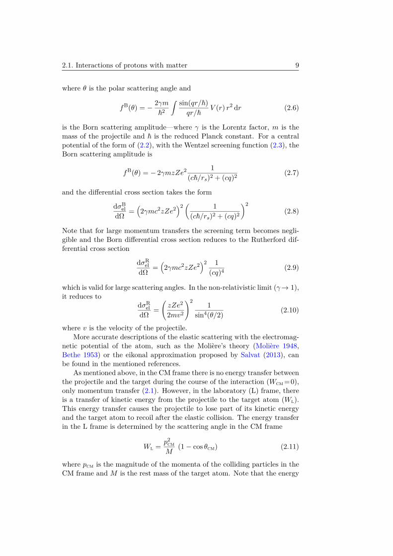
where θ is the polar scattering angle and
fB(θ) = − 2γm~2
∫ sin(qr/~)qr/~
V (r) r2 dr (2.6)
is the Born scattering amplitude—where γ is the Lorentz factor, m is themass of the projectile and ~ is the reduced Planck constant. For a centralpotential of the form of (2.2), with the Wentzel screening function (2.3), theBorn scattering amplitude is
fB(θ) = − 2γmzZe2 1(c~/rs)2 + (cq)2 (2.7)
and the differential cross section takes the form
dσBel
dΩ =(2γmc2zZe2
)2( 1
(c~/rs)2 + (cq)2
)2(2.8)
Note that for large momentum transfers the screening term becomes negli-gible and the Born differential cross section reduces to the Rutherford dif-ferential cross section
dσRel
dΩ =(2γmc2zZe2
)2 1(cq)4 (2.9)
which is valid for large scattering angles. In the non-relativistic limit (γ→ 1),it reduces to
dσRel
dΩ =(zZe2
2mv2
)2 1sin4(θ/2)
(2.10)
where v is the velocity of the projectile.More accurate descriptions of the elastic scattering with the electromag-
netic potential of the atom, such as the Molière’s theory (Molière 1948,Bethe 1953) or the eikonal approximation proposed by Salvat (2013), canbe found in the mentioned references.
As mentioned above, in the CM frame there is no energy transfer betweenthe projectile and the target during the course of the interaction (Wcm =0),only momentum transfer (2.1). However, in the laboratory (L) frame, thereis a transfer of kinetic energy from the projectile to the target atom (Wl).This energy transfer causes the projectile to lose part of its kinetic energyand the target atom to recoil after the elastic collision. The energy transferin the L frame is determined by the scattering angle in the CM frame
Wl = p2cmM
(1− cos θcm) (2.11)
where pcm is the magnitude of the momenta of the colliding particles in theCM frame and M is the rest mass of the target atom. Note that the energy

10 Chapter 2. Theory
transfer is zero for θcm = 0 (forward scattering) and reaches its maximumfor θcm =π (back scattering)
Wmax = 2 p2cmM
(2.12)
In the non-relativistic limit, which is the scenario that applies to protontherapy, it may be approximated by
Wmax = 4T mM
(m+M)2 (2.13)
where T is the kinetic energy of the projectile. Making use of equation (2.11),the differential cross section may be expressed in form of energy loss as
dσeldW
∣∣∣∣L
= 2π Mp2
dσeldΩ
∣∣∣∣cm. (2.14)
A quantity of interest in proton therapy is the nuclear stopping power,Snuc, which is defined as the average energy loss per unit path length dueto elastic collisions with the electromagnetic potential of the atom (Seltzeret al. 2011)
Snuc.= N
∫ Wmax
0W
dσeldW dW (2.15)
whereN is the number of target atoms (or molecules in compound materials)per unit volume. Note that the nuclear stopping power has nothing to dowith the proton interactions with the nuclear potential, but with the elasticscattering with the electromagnetic potential of the screened nucleus. Thenuclear stopping power is only important at very low energies. In water,its contribution to the total stopping power reaches the level of 1% onlyat kinetic energies below 20 keV (Berger et al. 1993), totally irrelevant toproton therapy.
Another quantity of interest is the so-called scattering power, Θ, which isdefined as the average angular deflection per unit path length due to elasticcollisions (Salvat 2014)
Θ .= 2N∫
(1− cos θ) dσeldΩ dΩ = 2
λ(1− 〈cos θ〉) (2.16)
where λ = 1/Nσel is the mean free path length between consecutive elasticinteractions. Note that for small scattering angles (θ1), Θ ≈ 〈θ2〉/λ.
Inelastic scattering
This section is based on ICRU Report No. 49 (Berger et al. 1993). Inaddition to elastic interactions, protons also interact inelastically with theatomic electrons, leading to the excitation and ionization of the target atoms.

2.1. Interactions of protons with matter 11
Inelastic collisions are the dominant mechanism of energy loss for protonsin matter.
One of the most important quantities in proton therapy is the electronicstopping power, Sel, which is defined as the average energy loss per unit pathlength due to inelastic collisions with the atomic electrons in the medium(Seltzer et al. 2011)
Sel.= N
∫ Wmax
0W
dσindW dW (2.17)
where (dσin/dW ) is the differential cross section for inelastic collisions. Notethat here the terminology recommended by ICRU Report No. 85 (Seltzeret al. 2011), with the suffix ‘el’ for electronic, has nothing to do with elasticcollisions.
The electronic stopping power of a charged particle may be expressed as
Sel = N 4πz2Ze4
mev2 L(β) (2.18)
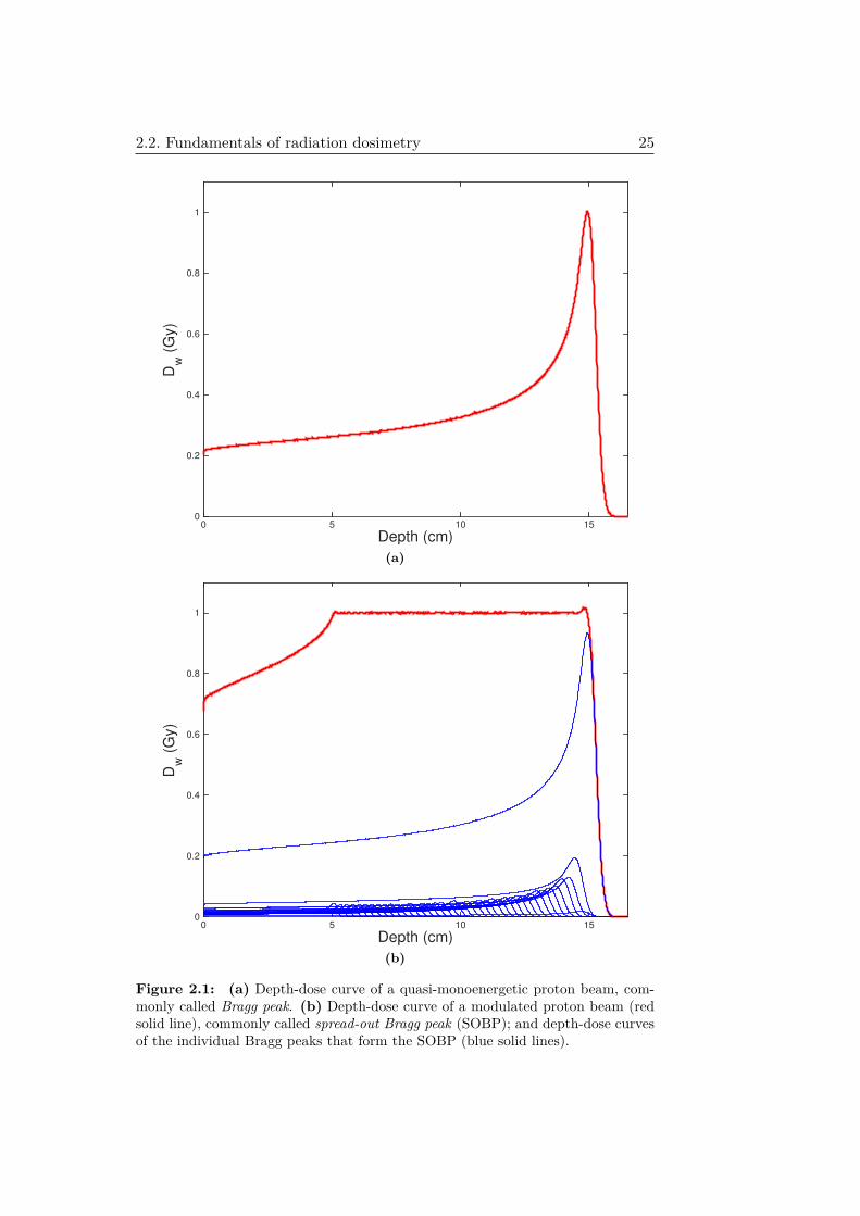
where N is the number of target atoms (or molecules in a compound ma-terial) per unit volume, z is the atomic number of the projectile, Z is theatomic number of the target atom, e is the charge of the electron, me isthe rest mass of the electron, v is the velocity of the projectil and L(β) isa quantity called stopping number, which is typically expressed in terms ofthe projectile velocity in units of the speed of light (β = v/c). The quan-tities preceding the stopping number take into account the gross featuresof the energy-loss process, whereas L takes into account the fine details.Note that, the electronic stopping power (2.18) is inversely proportional tov2. That is, the slower the projectile, the more energy is transferred to themedium. This behaviour explains, in part, the characteristic shape of proton(and charged-particles heavier than protons) energy deposition in depth, theso-called Bragg peak—see figure 2.1(a).
In the Bethe formulation of the electronic stopping power, the stoppingnumber may be expressed as (Berger et al. 1993)
L0(β) = 12 ln
(2mec
2β2Wmax1− β2
)− β2 − ln I − C
Z− δ
2 (2.19)
where I is the mean excitation energy of the medium, C/Z is the shellcorrection and δ/2 is the density effect correction. Wmax is the largestpossible energy loss in a single collision with a free electron, and it is givenby
Wmax = 2mec2β2
1− β2
[1 + 2γme
m+(me
m
)2]−1
(2.20)
where m is the mass of the projectile. Do not mix up with equation (2.12),which applies to elastic collisions. In the high-energy limit (γ →∞), Wmax

12 Chapter 2. Theory
approaches to the kinetic energy of the projectile, regardless of its mass.In the non-relativistic limit (γ → 1), which is the scenario that applies toproton therapy,
Wmax ≈ 2mev2 = 4
(me
m
)T. (2.21)
In the case of protons (mp ≈ 1836me), Wmax ∼ E/450.The Bethe formulation of the stopping-power (Bethe 1930) was derived
on the basis of the first-order Born approximation—i.e. it is valid for projec-tiles with large velocities, as compared to the velocity of the atomic electrons.As the velocity of the projectile decreases, the cross sections for inelastic scat-tering with the electrons in the deepest shells (K-shell, L-shells, etc.) start tovanish. The shell correction term (C/Z) in equation (2.19) takes this effectinto account. In the case of protons in water, the contribution of the shellcorrection to L reaches the level of 1% only for T < 10 MeV (Andreo et al.2013). Finally, the density effect correction term (δ/2) takes into accountthat the passage of a projectile polarizes the medium and this polarizationresults in a reduction of the stopping-power. Unlike the shell correction, thedensity effect correction is only relevant at high-energies (T > mc2). Forinstance, in the case of protons in water, its contribution to L reaches thelevel of 1% only for T > 1 GeV (Andreo et al. 2013).
Furthermore, two more terms are typically added to the Bethe formu-lation of the stopping number (2.19): the Barkas correction (zL1) and theBloch correction (z2L2) (Berger et al. 1993)
L(β) = L0(β) + z L1(β) + z2 L2(β) (2.22)
These terms take into account additional departures from the first-orderBorn approximation and are important only for low projectile velocities.For example, in the case of protons in water, their contribution to L reachesthe level of 1% only for T < 3 MeV (Andreo et al. 2013).
2.1.2 Nuclear interactions
Nuclear interactions refer to the interactions of protons with the nuclearpotential. Unlike electromagnetic interactions, in which the interaction po-tential is known, nuclear forces are only described approximately. Evaluatednuclear cross sections are based on a combination of experimental data andtheoretical models optimized to reproduce the experiments (Chadwick et al.2000). Thus, in this section, proton nuclear interactions will only be de-scribed qualitatively.
As electromagnetic interactions, nuclear interactions may also be classi-fied in elastic and inelastic collisions. In this case, inelastic nuclear inter-actions not only lead to the excitation of target nuclei, but also to nuclearfragmentation and particle transfer reactions.

2.1. Interactions of protons with matter 13
In the field of proton therapy, the effect of elastic nuclear interactions—orinelastic nuclear interactions leading to a mild excitation of target nuclei—is,in general, very similar to the effect of electromagnetic interactions, i.e. theylead to a small energy loss and angular deflection of the proton projectile.The exception are elastic nuclear interactions with the hydrogen nuclei inthe medium. In this particular case, the two outgoing protons (the inci-dent proton and the target hydrogen nucleus) share the kinetic energy ofthe projectile and they may exit the collision with large scattering angles(Gottschalk 2012).
On the contrary, inelastic nuclear interactions produce a very differenteffect than electromagnetic interactions: they “remove” protons from thebeam and they deposit part of their energy outside the beam path. In pro-ton therapy argot, primary protons refer to those protons that have sufferedelectromagnetic interactions only; whereas secondary protons typically referto those protons resulting from inelastic nuclear interactions. More in de-tail, inelastic nuclear interactions produce the following types of secondaryparticles:
(i) Secondary protons. These are typically low-energy protons with largescattering angles. They deposit their energy up to few centimetresaway from the interaction point.
(ii) Neutral particles (photons and neutrons). Typically these particlesdeposit their energy far from the primary beam path.
(iii) Charged particles heavier than protons (mainly 2H, 3H and α-particles)and recoil nuclei. These particles have very short ranges and, there-fore, they deposit their energy in the vicinity of the interaction point.Secondary particles heavier than α-particles are rare—see for instancefigure 3.2.
In the energy range relevant to proton therapy, total cross sections forinelastic nuclear scattering are nearly constant with energy, except at lowenergies where they increase before falling to zero (Chadwick et al. 2000,Gottschalk 2012). This increase in the total cross sections for inelastic nu-clear scattering with decreasing energy is similar to the increase in the to-tal cross section for inelastic electromagnetic scattering—which makes theprobability of inelastic nuclear interaction, with respect to other interactionmechanisms, nearly constant with proton energy.
In proton therapy we are sometimes interested in assessing the probabil-ity of a proton suffering an inelastic nuclear interaction at some point of itstrack and being therefore “removed” from the primary beam. As mentionedabove, the total cross section for inelastic nuclear scattering is approximatelyconstant with energy. On a first approximation, the probability of a pro-ton suffering an inelastic nuclear interaction per unit path length may also

14 Chapter 2. Theory
be considered nearly constant—as a rule of thumb, this probability is com-monly taken as 1% per cm. Thus, the higher the initial kinetic energy ofthe proton beam, the longer the range of the protons and, therefore, thehigher the percentage of protons suffering an inelastic nuclear interaction atsome point of their track and being removed from the primary beam. At thevery end of range, i.e. in the Bragg peak region, the probability of inelasticnuclear interaction falls to zero at the same time that the probability of in-elastic electromagnetic interaction increases drastically—see equation (2.18).

2.2. Fundamentals of radiation dosimetry 15
2.2 Fundamentals of radiation dosimetryThis section describes, in brief, the fundamental quantities, theories andprotocols that form the basis of current radiation dosimetry of clinical protonbeams.
2.2.1 Fundamental quantities
This section is based on ICRU Report No. 85 (Seltzer et al. 2011). It sum-marizes only those quantities relevant to the radiation dosimetry of clinicalproton beams.
Fluence
Let N be the expectation value of the number of particles incident on asphere of cross-sectional area da. Then the fluence, Φ, is defined as
Φ = dNda (2.23)
and its units are m−2. The use of a sphere of cross-sectional area da expressesthe fact that, in the definition of fluence, one considers an area da alwaysperpendicular to the direction of each particle.
An alternative, and equivalent, definition of fluence is
Φ = dldV (2.24)
where dl is (the expectation value of) the sum of all the particle track lengthsin an infinitesimal volume dV .
Energy imparted
The energy imparted, ε, in a given volume is defined as
ε = εin − εout +Q (2.25)
where εin is the sum of the kinetic energy of all the ionizing particles enteringthe volume, εout is the sum of the kinetic energy of all the ionizing particlesexiting the volume, and Q is the conversion of rest mass in kinetic energyin the volume (Q > 0: rest mass converted to kinetic energy; Q < 0: kineticenergy converted to rest mass).
Absorbed dose
The absorbed dose,D, is a point quantity defined from an stochastic quantity,ε. It is defined as the expected value of the energy imparted, dε, in a volumedV of mass dm
D = dεdm (2.26)

16 Chapter 2. Theory
i.e. is the expected value of the energy imparted per unit mass. Its unit isthe gray, Gy = J kg−1.
Stopping power
The stopping power, S, also called linear stopping power, is a quantity de-fined for charged particles only. As mentioned above in section 2.1.1, it isdefined as the average kinetic energy loss per unit path length, in a given ma-terial. Alternatively to equations (2.15) and (2.17), it may also be expressedmacroscopically as
S = dEdl (2.27)
with units of J m−1 or, more commonly, MeV cm−1. The total stoppingpower, S, may also be expressed as the sum of its independent components:S = Sel+Srad+Snuc; where Sel is the electronic stopping power due to inelas-tic electromagnetic interactions with the atomic electrons (2.17), Srad is theradiative stopping power due to bremsstrahlung emission in the electric fieldsof the atomic nuclei and electrons, and Snuc is the nuclear stopping powerdue to elastic electromagnetic interactions with the atomic nuclei (2.15).Note that, in the frame of clinical proton therapy, the relevant quantity isSel. More commonly used in radiation dosimetry is the mass stopping power,which is defined as the ratio between the stopping power and the materialmass density, S/ρ.
Linear energy transfer
The linear energy transfer or restricted linear electronic stopping power, L∆,of a given charged particle in a given material is defined as
L∆ = dE∆dl (2.28)
where dE∆ is the average energy loss by the charged particle in inelasticelectromagnetic collisions with the atomic electrons, minus the sum of thekinetic energy of all secondary electrons with kinetic energy E > ∆. Itsunits are J m−1 (or more commonly MeV cm−1). This definition expressesthe following energy balance: energy lost by the primary charged particlein inelastic electromagnetic interactions with the atomic electrons, minusthe enegy carried away by energetic secondary electrons with initial kineticenergy E > ∆, equals to energy “deposited locally”. That is, while Seldescribes the energy ‘lost’ by the charged particle, L∆ describes the energy‘deposited locally’ (i.e. in the vicinity of the interaction point) by the chargedparticle. Note that L∆ includes the binding energy of atomic electrons for allinteractions. As a consequence, L0 refers to the energy loss (per unit pathlength) due to inelastic electromagnetic interactions that lead to atomicexcitations only (no ionization), whereas L∞=Sel.
2.2. Fundamentals of radiation dosimetry 17
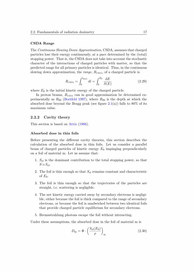
CSDA Range
The Continuous Slowing Down Approximation, CSDA, assumes that chargedparticles lose their energy continuously, at a pace determined by the (total)stopping power. That is, the CSDA does not take into account the stochasticcharacter of the interactions of charged particles with matter, so that thepredicted range for all primary particles is identical. Thus, in the continuousslowing down approximation, the range, Rcsda, of a charged particle is
Rcsda =∫ lmax
0dl =
∫ E0
0
dES(E) (2.29)
where E0 is the initial kinetic energy of the charged particle.In proton beams, Rcsda can in good approximation be determined ex-
perimentally as R80 (Bortfeld 1997), where R80 is the depth at which theabsorbed dose beyond the Bragg peak (see figure 2.1(a)) falls to 80% of itsmaximum value.
2.2.2 Cavity theory
This section is based on Attix (1986).
Absorbed dose in thin foils
Before presenting the different cavity theories, this section describes thecalculation of the absorbed dose in thin foils. Let us consider a parallelbeam of charged particles of kinetic energy E0 impinging perpendicularlyon a foil of material m. Let us assume that:
1. Sel is the dominant contribution to the total stopping power, so thatS'Sel.
2. The foil is thin enough so that Sel remains constant and characteristicof E0.
3. The foil is thin enough so that the trajectories of the particles arestraight, i.e. scattering is negligible.
4. The net kinetic energy carried away by secondary electrons is negligi-ble, either because the foil is thick compared to the range of secondaryelectrons, or because the foil is sandwiched between two identical foilsthat provide charged particle equilibrium for secondary electrons.
5. Bremsstrahlung photons escape the foil without interacting.
Under these assumptions, the absorbed dose in the foil of material m is
Dm = Φ ·(Sel(E0)
ρ
)m
(2.30)

18 Chapter 2. Theory
where Φ is the fluence of charged particles in the foil and (Sel(E0)/ρ)m isthe mass electronic stopping power of the charged particle in the materialm, evaluated at E0.
If the incident beam is polyenergetic, the absorbed dose in the foil is
Dm =∫ Emax
0Φ(E)
(Sel(E)ρ
)m
dE (2.31)
where Φ(E) is the distribution of fluence with respect to the energy ofcharged particles in the foil.
Bragg–Gray theory
Cavity theories study the relationship between the absorbed dose in a ho-mogeneous cavity inside a homogeneous medium, Dcav, and the absorbeddose at a point in the medium in the absence of the cavity, Dm.
In particular, the Bragg–Gray theory is based on the following two as-sumptions:
1. The size of the cavity is small compared to the range of the chargedparticles that cross it, so that the cavity does not perturb the fluenceof charged particles in the medium.
2. The absorbed dose in the cavity is deposited only by the charged par-ticles that cross it.
If these two assumptions (also called Bragg–Gray conditions) are ful-filled, the ratio between the absorbed dose in the medium and the absorbeddose in the cavity is
DmDcav
=∫ Emax
0 Φm(E) (Sel(E)/ρ)m dE∫ Emax0 Φm(E) (Sel(E)/ρ)cav dE
≡ sBGm,cav (2.32)
where Φm(E) is the distribution of fluence with respect to the energy ofprimary charged particles in the medium and Sel is the electronic stoppingpower. The last equality defines the Bragg–Gray medium/cavity stopping-power ratio, sBG
m,cav.Note that Bragg–Gray theory is based on equation (2.31) and, therefore,
it is also based on the underlying assumptions described in the previoussection. In particular, it assumes that secondary electrons deposit theirenergy locally or the existence of charged particle equilibrium for secondaryelectrons.
Spencer–Attix theory
The Spencer–Attix cavity theory is a refinement of the Bragg–Gray theory.Although it keeps on assuming that the cavity does not perturb the fluence

2.2. Fundamentals of radiation dosimetry 19
of charged particles in the medium, it takes into account that secondaryelectrons do not deposit all their energy locally.
The Spencer–Attix theory was initially derived assuming that the onlycharged particles that contributed significantly to the absorbed dose in themedium were electrons. In this context, it introduces the parameter ∆,which is defined as the mean energy of the electrons with a sufficient rangeto cross the cavity. Based on this parameter, a distinction is made betweensecondary electrons with kinetic energy E<∆, which are assumed to depositall their kinetic energy in the cavity, and secondary electrons with kineticenergy E>∆ (i.e. with sufficient energy to cross and leave the cavity), whichdeposit part of their kinetic energy outside the cavity.
According to Spencer–Attix cavity theory, the ratio between the ab-sorbed dose in the medium and the absorbed dose in the cavity is
DmDcav
=∫ Emax
∆ Φm(E) (L∆(E)/ρ)m dE + Φm(∆) (Sel(∆)/ρ)m ∆∫ Emax∆ Φm(E) (L∆(E)/ρ)cav dE + Φm(∆) (Sel(∆)/ρ)cav ∆
≡ sSAm,cav
(2.33)where Φm(E) is the distribution of fluence with respect to the energy of allelectrons (primary and secondary) in the medium, L∆ is the linear energytransfer (2.28), and Sel is the electronic stopping power. The last term ofthe sum, Φ(∆) (Sel(∆)/ρ) ∆, is the so-called track-end contribution (Nahum1978), where Φ(∆) is the fluence evaluated at E = ∆ (not the distributionof fluence with respect to ∆). The last equality defines the Spencer–Attixmedium/cavity stopping-power ratio, sSA
m,cav.When not only electrons, but also other charged particles, contribute to
the absorbed dose in the medium, the above formulation of the Spencer–Attix theory (2.33) may be generalised as follows
sSAm,cav =
∑i
∫ Emax
Eicut
Φim(E) (L∆(E)/ρ)im dE + Φi
m(Eicut)(Sel(Eicut)/ρ
)imEicut
∑i
∫ Emax
Eicut
Φim(E) (L∆(E)/ρ)icav dE + Φi
m(Eicut)(Sel(Eicut)/ρ
)icav
Eicut
(2.34)where i are the different types of charged particles that contribute to theabsorbed dose in the cavity; Eicut is defined as the mean energy of the i-th particle type with a sufficient range to cross the cavity (for electrons,Ecut = ∆); Φi
m(E) is the distribution of the fluence with respect to theenergy of the i-th particle type in the medium; and (L∆/ρ)i and (Sel/ρ)iare the mass linear energy transfer and the mass electronic stopping power,respectively, of the i-th particle type.
Let us analyse equation (2.34) in more detail. The first term of thesum,
∫ EmaxEcut
Φ(E) (L∆(E)/ρ) dE, is the contribution of charged particles withkinetic energy E >Ecut. These charged particles lose part of their energydue to inelastic electromagnetic collisions with the atomic electrons, giving

20 Chapter 2. Theory
rise to secondary electrons. Note that L∆ implies that only those secondaryelectrons with kinetic energy E<∆ contribute to the absorbed dose at thatpoint. The second term of the sum is the contribution of the track-ends.Track-ends are charged particles with kinetic energy E<Ecut, whose trackends in the cavity and, therefore, they deposit all their energy in the cavity.
The final expression of the track-end contribution is derived as follows.A priori, the track-end contributions, in what follows abbreviated as TE, fora given charged particle type should be
TE =∫ Ecut
0Φ(E)
(L∆(E)ρ
)dE (2.35)
By definition, track-ends deposit all their energy in the cavity. Thus, L∆(E)=Sel(E). Additionally, in the continuous slowing down approximation, it canbe shown that, for a given energy, the fluence of primary charged particlesΦ(E) is inversely proportional to the stopping power S(E) (Sempau 2006).Thus, it satisfies that
Φ(E) = Φ(Ecut)Sel(Ecut)Sel(E) (2.36)
Hence, substituting in equation (2.35),
TE =∫ Ecut
0Φ(Ecut)
Sel(Ecut)Sel(E)
(Sel(E)ρ
)dE = Φ(Ecut)
(Sel(Ecut)
ρ
)Ecut
(2.37)
2.2.3 Ionization chambers
Air-filled ionization chambers are the reference detectors in the dosimetryof radiotherapy beams. They allow to determine the absorbed dose in themedium (typically water) from the direct measurement of the ionizationproduced in the cavity.
Perturbation factors
The determination of the absorbed dose in the medium with an ionizationchamber is based on the cavity theory. However, real ionization chambersdo not fulfil Bragg–Gray conditions with the level of accuracy needed inradiation therapy. In particular, they do not fulfil the requirement that thecavity should not perturb the fluence of charged-particles in the medium.For the particular case of clinical proton beams, one could assume that, on afirst approximation, this requirement is fulfilled by protons (as they undergolittle scattering); but not by the secondary electrons resulting from inelasticelectromagnetic interactions.

2.2. Fundamentals of radiation dosimetry 21
Thus, in order to keep on using the cavity theory formalism, the conceptof perturbation correction factor or simply perturbation factor, p, is intro-duced, so that the relationship between the absorbed dose in the mediumand the absorbed dose in the cavity is expressed as
Dm = Dcav sm,cav p (2.38)
Historically, the global perturbation factor of a given detector, p, hasbeen assumed to be the product of different and independent perturbationfactors, pi, i.e. p=
∏pi. Typical perturbation factors of ionization chambers
used in the dosimetry of external radiotherapy beams are pcav, pcel, pdis andpwall, which take into account that the cavity, the central electrode and thewall of the ionization chamber are not equivalent to the medium, typicallywater—see Andreo et al. (2000) for a detailed definition of these terms.
The assumption of independent perturbation factors is, nevertheless, de-batable. When the fluence of charged particles in both the medium andthe cavity is known, it is possible to calculate the global perturbation factorof a detector, avoiding the unnecessary assumption of different independentperturbation factors (Nahum 1996). From equation (2.38), and using thegeneralised Spencer–Attix theory (2.34), it follows that the global perturba-tion factor of a given detector is
p =
∑i
∫ Emax
Eicut
Φim(E) (L∆(E)/ρ)icav dE + Φi
m(Eicut)(Sel(Eicut)/ρ
)icav
Eicut
∑i
∫ Emax
Eicut
Φicav(E) (L∆(E)/ρ)icav dE + Φi
cav(Eicut)(Sel(Eicut)/ρ
)icav
Eicut
(2.39)where i are the different types of charged particles that contribute to theabsorbed dose in the cavity.
Finally, if the fluence of charged particles in both the medium and thedetector cavity is known, it is also unnecessary to split the proportionalitybetween Dm and Dcav in two factors: sm,cav and p. That is, the relationshipbetween the absorbed dose in the medium and the absorbed dose in thecavity may also be expressed as (Sempau et al. 2004)
Dm = Dcav · f (2.40)
where, using the generalised Spencer–Attix theory (2.34), it follows that
f =
∑i
∫ Emax
Eicut
Φim(E) (L∆(E)/ρ)im dE + Φi
m(Eicut)(Sel(Eicut)/ρ
)imEicut
∑i
∫ Emax
Eicut
Φicav(E) (L∆(E)/ρ)icav dE + Φi
cav(Eicut)(Sel(Eicut)/ρ
)icav
Eicut
(2.41)where, again, i extends over the different types of the charged particles thatcontribute to the absorbed dose in the medium and the cavity.

22 Chapter 2. Theory
Absorbed dose in the ionization chamber cavity
Ionization chambers collect the electric charge, Q, produced in the ionizationchamber cavity as a consequence of the ionization of the cavity medium,typically air. Theoretically speaking, the absorbed dose in air, Dair, in theionization chamber cavity could be determined from the collected electriccharge (assuming that all produced charge is collected) as follows
Dair = Q
v ρair
Waire
(2.42)
where v is the sensitive volume of the ionization chamber, ρair is the densityof air, e is the charge of the electron and Wair is the mean energy needed tocreate an ion pair in air.
In practice, however, the sensitive volume of the ionization chamberstypically used in the dosimetry of radiotherapy beams is not known withsufficient accuracy. Thus, in order to determine the absorbed dose to air, ordirectly to water, with sufficient accuracy, one has to resort to the calibrationof ionization chambers. This point is addressed in the following section.
2.2.4 IAEA TRS-398 Code of Practice
The IAEA TRS-398 Code of Practice is an international consensus documentthat issues recommendations for the determination of the absorbed dose towater in external radiotherapy beams. This section of the thesis covers allthe points relevant to clinical proton beams, i.e. the formalism based onstandards of absorbed dose to water, the quality index for proton beamsand the reference conditions for the determination of the absorbed dose towater in proton beams. It is based on Andreo et al. (2000).
ND,w based formalism
The absorbed dose to water in a beam quality Q, Dw,Q, in the absence ofthe ionization chamber, is given by
Dw,Q = MQND,w,Q0 kQ,Q0 (2.43)
where MQ is the reading of the ionization chamber corrected for all thequantities of influence (except for the beam quality), ND,w,Q0 is the calibra-tion coefficient of the ionization chamber in terms of absorbed dose to waterin the reference beam quality Q0, and kQ,Q0 is the beam quality correctionfactor. kQ,Q0 corrects for the different response of the ionization chamber inthe user beam quality Q and the calibration beam quality Q0. The deter-mination of the absorbed dose to water in a user beam quality Q with anionization chamber calibrated in a reference beam quality Q0 that might bedifferent from the user beam quality is commonly called reference dosimetry.

2.2. Fundamentals of radiation dosimetry 23
The raw reading of the ionization chamber should be corrected for all thequantities that influence the quantity under measurement—in this case, thecollected charge—using appropriate correction factors, ki. These influencequantities, and their corresponding correction factors, are: pressure andtemperature of the chamber air (kTP), humidity of air (kh), electrometercalibration (kelec), voltage polarity (kpol) and ion recombination (ks). Thesefactors are described in detail in Andreo et al. (2000).
The calibration coefficient in terms of absorbed dose to water in thereference beam quality Q0 is given by
ND,w,Q0 = Dw,Q0
MQ0(2.44)
where Dw,Q0 is the absorbed dose to water at the reference measurementpoint in the reference beam quality Q0 under reference conditions, and MQ0
is the reading of the ionization chamber corrected for all the influence quan-tities mentioned above. Typically, the reference beam quality is 60Co gammaradiation.
Beam quality correction factor
As mentioned above, the beam quality correction factor, kQ,Q0 , corrects forthe different response of the ionization chamber in the user beam qualityQ and the calibration beam quality Q0. It is defined as the ratio of theionization chamber calibration coefficients (in terms of absorbed dose towater) at the beam qualities Q and Q0
kQ,Q0 = ND,w,QND,w,Q0
= Dw,Q/MQ
Dw,Q0/MQ0(2.45)
Ideally, beam quality correction factors should be determined experimen-tally in a Primary Standards Dosimetry Laboratory (PSDL) with a beamquality-independent metrology primary standard, such as a water calorime-ter. However, such an experimental determination is seldom possible inPSDLs, mainly because of the difficulty in reproducing the user beam qual-ity. This is certainly the case for proton beams, since at present no PSDLis equipped with proton beam qualities. When experimental beam qualitycorrection factors are not available, they can also be calculated theoreticallyas (Andreo 1992)
kQ,Q0 = sw,air,Qsw,air,Q0
Wair,QWair,Q0
pQpQ0
(2.46)
where sw,air is the Spencer–Attix water/air stopping-power ratio (defined insection 2.2.2), Wair is the mean energy needed to create an ion pair in air(defined in section 2.2.3) and p is the perturbation correction factor of theionization chamber (also defined in section 2.2.3).

24 Chapter 2. Theory
Finally, and this is not included in IAEA TRS-398, Sempau et al. (2004)proposed an alternative and more accurate approach to the calculationof beam quality correction factors, which exploits the potential of MonteCarlo simulation techniques. From the principles of cavity theory (see sec-tion 2.2.2), it follows from equation (2.46) that beam quality correctionfactors can also be calculated as
kQ,Q0 = fQfQ0
Wair,QWair,Q0
= (Dw/Dair)Q(Dw/Dair)Q0
Wair,QWair,Q0
(2.47)
where f is an ionization chamber-specific and beam quality-dependent fac-tor, defined above in equation (2.40), that establishes the proportionalitybetween the absorbed dose to water at the reference point of measurementin the absence of the detector (Dw) and the average absorbed dose to air inthe ionization chamber sensitive volume (Dair).
Due to a lack of experimental data and Monte Carlo calculated datausing equation (2.47) at the time of publication, IAEA TRS-398 uses equa-tion (2.46) to calculate the beam quality correction factors for clinical protonbeams. 60Co gamma radiation is taken as reference beam quality. In thiscase, the subscript Q0 in kQ,Q0 is typically omitted. In what follows, wewill adopt this nomenclature. The values entering in equation (2.46) are thefollowing:
• For 60Co gamma radiation, IAEA TRS-398 adopts the water/air stop-ping-power ratio value of sw,air,Q0 = 1.133 (Andreo et al. 1986) andWair,Q0 = 33.97 eV. The perturbation correction factors are ionizationchamber-specific and are tabulated for a wide range of cylindrical andplane-parallel ionization chambers.
• For proton beams, IAEA TRS-398 adopts the water/air stopping-power ratios calculated by Medin & Andreo (1997) for monoenergeticproton beams and Wair,Q = 34.23 eV. Due to a lack of experimentaland Monte Carlo data, perturbation correction factors are taken to beunity.
All the values entering into equation (2.46) are associated with an estimateduncertainty. Table 2.1 shows the estimates of the relative standard uncer-tainty of all the values entering into the IAEA TRS-398 calculation of kQfactors for proton beams, as well as the combined standard uncertainty ofthe kQ factors themselves.
Beam quality index
At the time of IAEA TRS-398 publication, the vast majority of proton ther-apy treatments were delivered with modulated proton beams, which gener-ate the so-called spread-out Bragg peak (SOBP) fields—see figure 2.1(b). A
2.2. Fundamentals of radiation dosimetry 25
Depth (cm)0 5 10 15
Dw
(G
y)
0
0.2
0.4
0.6
0.8
1
(a)
Depth (cm)0 5 10 15
Dw
(G
y)
0
0.2
0.4
0.6
0.8
1
(b)
Figure 2.1: (a) Depth-dose curve of a quasi-monoenergetic proton beam, com-monly called Bragg peak. (b) Depth-dose curve of a modulated proton beam (redsolid line), commonly called spread-out Bragg peak (SOBP); and depth-dose curvesof the individual Bragg peaks that form the SOBP (blue solid lines).

26 Chapter 2. Theory
Table 2.1: Estimated relative standard uncertainty of all the components enteringinto the calculation of kQ and combined relative standard uncertainty of the kQ
factors for proton beams. All values are in %. A distinction is made betweencylindrical and plane-parallel ionization chambers. Adapted from Andreo et al.(2000).
Cylindrical Plane-parallel
60Co γ-rays
sw,air 0.5Assignment sw,air to Q0 0.1Wair 0.2pQ0 0.6 1.5
Protons
sw,air 1.0Assignment sw,air to Q 0.3Wair 0.4pQ 0.8 0.7
kQ 1.6 2.1
spread-out Bragg peak is the superposition of quasi-monoenergetic protonbeams of different energy and intensity so that it creates a region of uniformdose in depth. The beam quality index for proton beams is the so-calledresidual range, Rres. At the measurement depth z the residual range isdefined as
Rres = Rp − z (2.48)
where Rp is the practical range, which is defined as the depth at which theabsorbed dose beyond the Bragg peak or SOBP falls to 10% of its maximumvalue. Note that, based on this definition, the beam quality Q is not uniquefor a particular proton beam, but it is also determined by the measurementdepth.
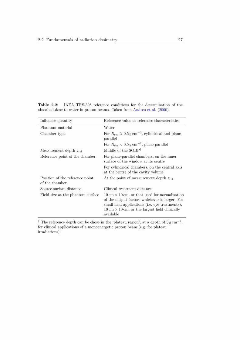
Reference conditions for the determination of the absorbed doseto water
Table 2.2 summarizes the reference conditions for the determination of theabsorbed dose to water in proton beams recommended by IAEA TRS-398.Note, from the recommendation on the measurement depth, that theseconditions were mainly thought for modulated proton beams. However,the footnote in table 2.2 opens the door also to monoenergetic, or quasi-monoenergetic, proton beams. The terms quasi-monoenergetic or pseudo-monoenergetic will be used indistinctively in this work to stress that clinicalproton beams are not monoenergetic, but they have an inherent initial en-ergy spread.
2.2. Fundamentals of radiation dosimetry 27
Table 2.2: IAEA TRS-398 reference conditions for the determination of theabsorbed dose to water in proton beams. Taken from Andreo et al. (2000).
Influence quantity Reference value or reference characteristics
Phantom material WaterChamber type For Rres > 0.5 g cm−2, cylindrical and plane-
parallelFor Rres < 0.5 g cm−2, plane-parallel
Measurement depth zref Middle of the SOBP†
Reference point of the chamber For plane-parallel chambers, on the innersurface of the window at its centreFor cylindrical chambers, on the central axisat the centre of the cavity volume
Position of the reference point At the point of measurement depth zrefof the chamberSource-surface distance Clinical treatment distanceField size at the phantom surface 10 cm× 10 cm, or that used for normalisation
of the output factors whichever is larger. Forsmall field applications (i.e. eye treatments),10 cm× 10 cm, or the largest field clinicallyavailable
† The reference depth can be chose in the ‘plateau region’, at a depth of 3 g cm−2,for clinical applications of a monoenergetic proton beam (e.g. for plateauirradiations).

28 Chapter 2. Theory
2.3 A little touch of Monte Carlo simulation
This section presents briefly and qualitatively the basic concepts of MonteCarlo simulation methods applied to radiation transport. It is mainly adaptedfrom Salvat (2014). For a more comprehensive introduction to Monte Carlosimulation applied to the transport of radiation, the reader is referred toBielajew (2001) or Salvat (2014).
Monte Carlo methods are a class of numerical methods that rely onthe repeated sampling of random numbers to obtain a numerical result. InMonte Carlo simulation of radiation transport, the track of a particle isviewed as a random sequence of free flights that end with an interactionevent where the particle loses energy, suffers an angular deflection and, oc-casionally, produces secondary particles. That is, each step of a particletrack is characterised by the following variables: (i) step length (or freepath) between successive interaction events, (ii) type of interaction takingplace, and (iii) energy loss and angular deflection in that particular event(and initial state of the secondary particles, if any). Each of these variables(either discrete or continuous) are sampled from a probability distributionfunction. These probability density functions are determined by the dif-ferential cross sections for the relevant interaction mechanisms. Thus, theaccuracy of a Monte Carlo calculation is limited by the accuracy of the in-teraction models it is based on. The precision of the calculation, however,can always be improved by simulating a larger number of histories1.
The simulation scheme described above, in which the track of a particleis simulated interaction by interaction, is known as detailed simulation. Sucha simulation scheme is feasible for particles such as photons, which undergoa reasonably low number of interactions per track, but not for high-energycharged particles, which may undergo millions of collisions before stopping.Fortunately in the case of charged particles most of these collisions involvesmall energy losses and small angular deflections, so that the effect (i.e. en-ergy loss and angular deflection) of many interactions can be summed upand described approximately in a single simulation step. In this simulationstrategy, the total energy loss and angular deflection at the end of each step iscalculated from macroscopic stopping and multiple Coulomb scattering the-ories, respectively, and not from differential cross sections. This condensedsimulation strategy is called, according to the terminology introduced byBerger (1963), complete grouping or class I simulation scheme.
There is a third approach to the simulation of charged particle transportcalled mixed or class II simulation scheme (Berger 1963). This approachdistinguishes between soft collisions (i.e. interactions with small energy lossand angular deflection) and hard collisions (i.e. interactions with a large
1The term history, or event, refers typically to the tracks of a primary particle and allits descendants.

2.3. A little touch of Monte Carlo simulation 29
energy loss or large angular deflection). Mixed simulation combines thedetailed simulation of hard events with condensed simulation of soft events.The boundary between soft and hard events is typically set by user-definablethreshold values.
The Monte Carlo method applied to radiation transport yields, exceptfor its inherent statistical uncertainty, the same information as the solutionof the Boltzmann transport equation, with the same interaction model. Theadvantage of Monte Carlo methods is that they are easier to implement,especially in complex geometries. The drawback is its random nature: allthe results are affected by statistical uncertainties, which can be reducedat the expense of increasing the number of histories simulated and, hence,the computation time. In this work, Monte Carlo methods are used to solvemacroscopic problems (e.g. the calculation of the absorbed dose) through thesimulation of microscopic events (the interaction of radiation with matter).

30 Chapter 2. Theory

Chapter 3
Spencer–Attixwater/mediumstopping-power ratios forproton pencil beams
This chapter is based on Gomà et al. (2013). It describes the Monte Carlocalculation of Spencer–Attix water/medium stopping-power ratios for pro-ton pencil beams, which are important for both the reference and rela-tive dosimetry of proton pencil beam. This work calculates water/mediumstopping-power ratios, as a function of depth and radial distance, for pro-ton energies ranging from 30 to 350 MeV and typical detection materials inproton therapy such as air, radiochromic film, gadolinium oxysulfide, siliconand lithium fluoride. Furthermore, it investigates the effect on the water/airstopping-power ratios of track-ends, particles heavier than protons, the meanexcitation energy of water and the initial energy spread of the beam.
3.1 Introduction
The commissioning of scanned proton pencil beams requires: (i) referencedose measurements to calibrate the beam monitor chambers, (ii) relativedose measurements, i.e. depth-dose curves and lateral dose profiles, to feedthe treatment planning system, and (iii) field-specific dose distributions mea-surements to validate the dose distribution predicted by the treatment plan-ning system.
According to IAEA TRS-398 (see section 2.2.4), the absorbed dose towater under reference conditions should be measured in water with a cylin-drical or plane-parallel ionization chamber. Depth-dose curves should also bemeasured in water (Andreo et al. 2000), with a large-diameter plane-parallel
31

32 Chapter 3. Water/medium stopping-power ratios
ionization chamber (Jones et al. 2007). Lateral dose profiles are typicallymeasured with high spatial resolution detectors, such as radiochromic films(Gillin et al. 2010) or scintillating screens coupled to a CCD camera (Pedroniet al. 2005). In what follows, and for the sake of simplicity, we will refer tothese latter detectors as scintillating screens. Alternatively, lateral dose pro-files may also be measured with a small volume ionization chamber (Gillinet al. 2010, Schwaab et al. 2011). Finally, field-specific dose distributionsare typically measured with two-dimensional detectors such as ionizationchamber matrices (Karger et al. 2010), radiochromic films (Albertini et al.2011) or scintillating screens (Boon et al. 2000).
All these measurements, performed with different detectors and detec-tion materials, will most likely be converted to absorbed dose to water.To correctly perform this step, it is essential to know the water/mediumstopping-power ratio of the detection material and the perturbation cor-rection factor of the detector. This chapter addresses the calculation ofthe water/medium stopping-power ratios (sw,med) for proton pencil beams,which are a property of the detection material and the radiation field. Thecalculation of perturbation correction factors, which are a property of thedetector and the radiation field, will be addressed in chapter 6 for ionizationchambers.
In the field of proton therapy, the largest contributions to the calcu-lation of stopping-power ratios have historically focused on the water/airstopping-power ratio (sw,air), because of its importance for reference dosime-try. Medin & Andreo (1997) calculated sw,air values for monoenergetic pro-ton beams from 50 to 250 MeV with their self-developed Monte Carlo codepetra—where nuclear inelastic processes were taken into account but onlyprotons (both primary and secondary) and delta-ray electrons were tracked.They found delta-ray electrons should be included in the calculation of sw,airwhereas alpha particles could be omitted. Later, Laitano & Rosetti (2000)calculated sw,air values for proton beams with a realistic energy spectra—with the fluka Monte Carlo code—and they found no significant differenceswith sw,air values obtained for monoenergetic beams. Finally, IAEA TRS-398 derived the sw,air values for passively-scattered proton beams.
Based on these past results, the aim of this chapter is to use Monte Carlosimulations:
1. To calculate sw,med values for the detection materials most commonlyused in the dosimetry of proton pencil beams. These detection ma-terials are: air (ionization chambers), radiochromic film (GafchromicEBT2/EBT3 active layer1) and gadolinium oxysulfide (Gd2O2S:Tb, ascintillating material). Silicon (Si) and lithium fluoride (LiF) were also
1According to the manufacturer, the active layers of EBT2 and EBT3 films are iden-tical. In what follows, and for the sake of simplicity, we will refer to the EBT2/EBT3active layer by simply EBT2.

3.2. Materials and methods 33
included for completeness. Special attention was paid to sw,air becauseof its importance in reference dosimetry.
2. To extend the energy range from 30 to 350 MeV, to take into accountthe upcoming generation of proton therapy beam delivery systems.
3. To investigate the influence of particles heavier than protons and track-ends on the calculation of the stopping-power ratios.
4. To investigate the effect of the initial energy spread of the beam onthe stopping-power ratios.
5. To investigate the dependence of sw,med on the radial distance (per-pendicular to the beam direction). This last point was inspired by theresults of Grassberger & Paganetti (2011) showing an increased LETin the penumbra region of clinical proton beams.
3.2 Materials and methods
This chapter calculates water/medium stopping power ratios by means ofthe Spencer–Attix cavity theory, i.e. using equation (2.34). An upper limitfor Eicut is typically defined as the mean energy of the i-th particle with asufficient residual range to cross the cavity. In this work, we set the size ofthe cavity equal to the typical mass-thickness of a plane-parallel ionizationchamber cavity, i.e. 2.5 · 10−4 g cm−2. This setting leads to an upper limitfor Ecut of 10 keV for electrons, 175 keV for protons, 250 keV for alphas,etc. For simplicity, we set ∆ = 10 keV for electrons and Ecut = 100 keV forprotons and heavier particles.
The calculation of the sw,med values was performed ‘off-line’. That is,we first calculated the distribution of the fluence with respect to the energywith Monte Carlo simulations and, afterwards, we calculated the sw,medvalues using equation (2.34). To overcome the potential deficiencies of an‘off-line’ calculation, we used a dense (∼ 103) logarithmic energy binning.For the Monte Carlo simulations, we used Gamos (Arce et al. 2014)—aMonte Carlo simulation software framework based on the Geant4 toolkit.As a reference beam, we simulated a zero-emittance beam (zero initial lat-eral spread and zero initial angular spread) with a zero initial energy spreadimpinging on a sufficiently large (15 cm-radius) cylindrical water phantom.We used the QGSP_BIC_EMY physics list (Cirrone et al. 2009), whichcombines the electromagnetic standard model for the electromagnetic pro-cesses, the binary cascade model for the hadronic inelastic processes, andan accurate tracking of electrons, hadrons and ions for dosimetry purposes.These physics settings have been proved to be suitable for the simulation ofproton therapy beams (Zacharatou-Jarlskog & Paganetti 2008). We set the

34 Chapter 3. Water/medium stopping-power ratios
production cuts for photons, electrons and positrons to 2.5µm—to be con-sistent with our setting for the size of the cavity. We scored the (averaged)fluence of charged particles in a disc of water of 0.1 mm of thickness and10 cm of radius, perpendicular to the beam axis. We chose a sufficientlylarge radius to capture all the secondary charged particles scattered at largeangles due to inelastic nuclear interactions. As mentioned before, the flu-ence was scored in a dense (∼ 103) set of logarithmic energy bins, fromEcut to Emax. We run as many particles as needed to achieve a standardstatistical uncertainty in the final sw,med values lower than 0.1%. The totaluncertainty, however, is much larger and it is mainly due to the uncertaintyin the mean excitation energy values (I-values) of the different media. Thispoint will be discussed later.
For the calculation of sw,med using equation (2.34), we first consideredonly the fluence of protons and electrons (Medin & Andreo 1997)—the in-fluence of heavier particles is investigated later. For all materials except forwater, we took the mass electronic stopping powers (Sel/ρ) for protons andelectrons directly from ICRU Report No. 49 (Berger et al. 1993) and ICRUReport No. 37 (Berger et al. 1984), respectively. When not tabulated, wecalculated them with the Bragg additivity rule as suggested in ICRU 37,i.e. taking the I-values for the condensed phase of the elements in the com-pound. For water, however, we took the Iw-value suggested by Andreo et al.(2013) (Iw = 78 eV), instead of the current ICRU 37 and ICRU 49 recom-mendation (Iw = 75 eV). Finally, the restricted linear electronic stoppingpowers (L∆) were calculated from Sel as suggested in ICRU 49.
We studied the effect of particles heavier than protons and track-endson the calculation of the water/air stopping-power ratio. In this case, allthe charged particles that crossed the cavity were scored. The calculation ofthe water/air stopping-power ratio included alpha particles and all the ionswith tabulated (Sel/ρ) values in ICRU Report No. 73 (Bimbot et al. 2005,Sigmund et al. 2009). These were the isotopes of lithium (6Li, 7Li, 8Li),beryllium (6Be, 7Be, 9Be, 10Be), boron (8B, 10B, 11B, 12B, 13B), carbon(10C, 11C, 12C, 13C, 14C, 15C), nitrogen (12N, 13N, 14N, 15N, 16N, 17N),oxygen (13O, 14O, 15O, 16O, 17O, 18O, 19O), fluorine (17F, 18F, 19F) andneon (20Ne). We included them in equation (2.34) as follows: for alphaparticles we calculated L∆; for heavier ions we assumed L∆ ≈ Sel. Thisassumption is based on the fact that, for a given energy, the heavier theprojectile, the lower the energy lost in a single collision with an electron inthe medium (see equation (2.21)), so the smallest the difference between L∆and Sel. In case this approximation was not sufficiently accurate, this wouldresult in an overestimation of the contribution of these heavier ions to sw,air.
The effect of the track-ends was simply assessed by calculating sw,air

3.3. Results and discussion 35
without the track-end term, i.e.
sw,air =
∑i
∫ Emax
Eicut
Φiw(E) (L∆(E)/ρ)iw dE
∑i
∫ Emax
Eicut
Φiw(E) (L∆(E)/ρ)iair dE
(3.1)
and comparing with the full equation (2.34). In this case, only the fluenceof protons and electrons was taken into account.
We also investigated the effect of the initial energy spread of the beamon the sw,air values in depth. We investigated a Gaussian initial (relative)energy spread, σE/E, of 1%, which is representative of the values that cannowadays be achieved in modern proton therapy facilities (Clasie et al. 2012).
Finally we studied sw,med as a function of the radial distance (perpen-dicular to the beam direction) at the depth of R80/2, which is a depth witha broad halo of secondary protons for all energies (Pedroni et al. 2005). Inthis case, the scoring volume was divided in concentric rings of width equalto 0.5σMCS, where σMCS is the standard deviation of the lateral spread ofthe beam in depth due to multiple Coulomb scattering (MCS). σMCS wascalculated at the depth of R80/2 using the generalized Fermi-Eyges multiplescattering theory (Safai et al. 2008).
3.3 Results and discussionFigure 3.1(a) shows the Spencer–Attix sw,air values as a function of depthin water for different proton energies (30, 70, 150, 230 and 350 MeV). Thedepth in water is normalized to the range (R80) of the proton beam. Thenumerical values are shown in table 3.1. As in Medin & Andreo (1997), itwas found that the peak-to-plateau ratio decreases with increasing energy—from 2.5% for 30 MeV beams to 1% for 350 MeV beams. This is due to therange straggling in water, which makes the proton energy spectrum at theBragg peak region much broader for high energies than for low energies.
Figure 3.1(b) shows a comparison of the Spencer–Attix sw,air values, for a150 MeV beam, obtained in this work with Geant4 and the values publishedby Medin & Andreo (1997) using petra. When using the same input data(Iw = 75 eV), an excellent agreement (within 0.1%) was found between thetwo Monte Carlo codes. When using Iw = 78 eV, we found differences from0.6% in the plateau region and up to 1% in the Bragg peak region. As alreadypointed out by other authors (Andreo 2009, Henkner et al. 2009, Vatnitskyet al. 2011), the uncertainty in the I-values is currently the largest sourceof uncertainty in the sw,air values. For relative dosimetry purposes however,the absolute sw,air values are not so critical; the only relevant quantitiesare the relative sw,air values along the beam range or, in other words, thepeak-to-plateau ratio. Still, it was found that Iw has a noticeable effect on

36 Chapter 3. Water/medium stopping-power ratios
Depth / R80
0.2 0.4 0.6 0.8 1
sw
,air
1.12
1.13
1.14
1.15
1.16
30 MeV 70 MeV150 MeV230 MeV350 MeV
(a)
Depth (cm)0 4 8 12 16
sw
,air
1.12
1.13
1.14
1.15
1.16
This work (Iw
=78eV)
This work (Iw
=75eV)
Medin and Andreo (1997)
(b)
Figure 3.1: (a) Spencer–Attix sw,air values as a function of depth for protonbeams of initial energy 30, 70, 150, 230 and 350 MeV. The values correspond toIw = 78 eV. (b) Comparison of the sw,air values obtained in this work with thevalues published by Medin & Andreo (1997) for a 150 MeV proton beam.

3.3. Results and discussion 37
Table 3.1: Spencer–Attix sw,air values as a function of depth for proton beams ofinitial energy 30, 70, 150, 230 and 350 MeV. The values correspond to Iw =78 eV.
Energy (MeV)
Depth/R80 30 70 150 230 350
0.100 1.131 1.130 1.130 1.129 1.1290.370 1.132 1.130 1.130 1.129 1.1290.600 1.132 1.131 1.130 1.130 1.1290.750 1.133 1.131 1.130 1.130 1.1300.840 1.133 1.132 1.130 1.130 1.1300.900 1.134 1.132 1.131 1.130 1.1300.937 1.136 1.133 1.131 1.131 1.1300.960 1.139 1.134 1.132 1.131 1.1310.975 1.145 1.137 1.133 1.132 1.1310.984 1.149 1.140 1.135 1.133 1.1321.000 1.152 1.144 1.138 1.136 1.1351.016 1.153 1.147 1.141 1.139 1.1371.025 1.153 1.149 1.142 1.139 1.137
R80 (cm) 0.90 4.11 15.87 31.92 66.62
the peak-to-plateau ratio. For instance, for the 30 MeV beam, the peak-to-plateau ratio ranged from 2.8% (for Iw =75 eV) to 2.0% (for Iw =78 eV); forthe 350 MeV beam, it ranged from 0.9% to 0.7%. The effect of the I-valueson sw,air decreases with increasing energy. This is due to the fact that, thehigher the energy of the projectile, the less relevant the I-value in the masselectronic stopping power of the projectile.
Figure 3.2 shows the distribution of the fluence of charged particles inwater with respect to the energy generated by a proton beam of initial energy150 MeV at the depth of R80/10 = 1.6 cm. It was found that the main con-
Table 3.2: Relative per cent contribution of the different charged particles to theabsorbed dose to water and, within parenthesis, relative per cent contribution of thetrack-ends to the dose deposited by that particle. The plateau region is representedby the depth of 0.1R80; the peak region, by 0.984R80, which corresponds roughlyto the depth of the maximum.
30 MeV 150 MeV 350 MeV
Plateau Peak Plateau Peak Plateau Peak
Protons 85.9 (0.0) 100 (0.2) 79.6 (0.0) 91.2 (0.0) 77.3 (0.0) 87.0 (0.0)Electrons 13.6 (39) 0.0 (78) 19.2 (26) 8.6 (54) 20.7 (23) 12.5 (40)Others 0.5 (0.1) 0.0 (3.0) 1.2 (0.5) 0.2 (0.3) 2.0 (0.4) 0.5 (0.4)

38 Chapter 3. Water/medium stopping-power ratios
E (MeV)10
-210
-110
010
110
2
Φw
(E)
(MeV
-1 c
m-2
)
10-10
10-8
10-6
10-4
10-2
100
ProtonsElectronsPositronsDeuteronsTritonsAlphasOthers
Figure 3.2: Distribution of the fluence of charged particles in water with respectto the energy per incident proton of initial energy 150 MeV at the depth of R80/10 =1.6 cm.
tribution to the fluence comes from both protons and electrons; whereas thefluence of heavier particles is several orders of magnitude lower. Figure 3.2also shows that the fluence of protons is clearly dominated by the primaryprotons and the fluence of electrons is clearly dominated by the proton-generated secondary electrons. The latter is shown by the drastic reductionof the electron fluence for E > Wmax, where Wmax is the largest possibleenergy loss of a proton in single collision with a free electron (2.21); in thiscase, Wmax ∼ 300 keV. The major contribution of protons and electrons tothe fluence does translate into a major contribution to the absorbed dose towater, as shown in table 3.2—where the relative contribution to Dw fromthe different charged particle species is shown. The significant contributionof the electrons to both the fluence and the absorbed dose to water, however,does not translate into a significant contribution to the sw,air values.
Figure 3.3 shows the effect of including different charged particles (pro-tons; both protons and electrons; and all charged particles) in the calculationof sw,air for different proton energies (30, 150 and 350 MeV). Systematic dif-ferences of the order of 0.1% were found when including electrons into equa-tion (2.34), but no further significant differences were found when includingthe rest of particles heavier than protons. A similar behaviour was found forthe track-ends. Table 3.2 also shows the relative contribution of the track-

3.3. Results and discussion 39
Depth / R80
0.2 0.4 0.6 0.8 1
sw
,air
1.12
1.13
1.14
1.15
1.16
30 MeV (protons) 30 MeV (protons + electrons) 30 MeV (all charged particles)150 MeV (protons)150 MeV (protons + electrons)150 MeV (all charged particles)350 MeV (protons)350 MeV (protons + electrons)350 MeV (all charged particles)
Figure 3.3: Spencer–Attix sw,air values as a function of depth for proton beamsof initial energy 30, 150 and 350 MeV. The solid lines include only protons, thedashed lines include protons and electrons, and the chain lines include all chargedparticles.
ends to the dose deposited by each type of particle, within parenthesis. Itwas found that, although electron track-ends can deposit up to 80% of thetotal dose deposited by the electrons, the minor role of the electrons in thesw,air values makes the contribution of these track-ends negligible. For pro-tons and heavier particles, the contribution of the track-ends to Dw (andtherefore to sw,air) was found to be negligible—at least for the cut-off energyof Ecut = 100 keV. Here, it is worth commenting on the need of includingelectrons in the calculation of the sw,air values. Medin & Andreo (1997)compared the Bragg-Gray sw,air values for protons with the Spencer–Attixsw,air values including both protons and electrons and they found differencesof about 0.5%. This work compares the Spencer–Attix sw,air values includ-ing protons and both protons and electrons and it found differences of only0.1%. This leads to the conclusion that, when using L∆ in the cavity in-tegral, as in equation (2.34), the inclusion of electrons in the calculation ofsw,air is, to a very good approximation, not necessary.
Figure 3.4 shows the effect of the initial energy spread of the beam onthe sw,air values as a function of depth in water for different proton energies(30, 150 and 350 MeV). A relative initial energy spread of 1% is compared

40 Chapter 3. Water/medium stopping-power ratios
Depth / R80
0.2 0.4 0.6 0.8 1
sw
,air
1.12
1.13
1.14
1.15
1.16
30 MeV (σE
/E = 0)
30 MeV (σE
/E = 1%)
150 MeV (σE
/E = 0)
150 MeV (σE
/E = 1%)
350 MeV (σE
/E = 0)
350 MeV (σE
/E = 1%)
Figure 3.4: Spencer–Attix sw,air values as a function of depth for proton beamsof initial energy 30, 150 and 350 MeV. The solid lines show proton beams withinitial σE/E = 0; the dashed lines show proton beams with initial σE/E = 1%.
to a zero initial energy spread. We found differences up to 0.5% in theBragg peak region and no significant differences in the plateau. We alsofound the effect of the initial energy spread decreases with increasing energy.This is due to the fact that, at low energies, the total energy spread at theBragg peak region is dominated by the initial energy spread of the beamwhereas, at high energies, it is dominated by the range straggling in water.Furthermore, for the highest energy beams—meant for proton radiography(Depauw & Seco 2011)—one could argue that the initial energy spread of thebeam has no effect on their relative dosimetry, since only the plateau regionis used clinically. However, attention should be paid to low energy beams,where a narrow initial energy spread is technically more challenging—atleast for cyclotron-based facilities—and its effect on the relative dosimetryshould not be overlooked.
Figure 3.5 shows the sw,med values as a function of depth in water fordifferent detection materials (air, EBT2, Gd2O2S:Tb, Si, LiF) and differentproton energies (30, 150 and 350 MeV). The sw,med values are normalizedto the entrance (R80/10) value. Table 3.3 shows the absolute numericalvalues—for EBT2, gadolinium oxysulfide, Si and LiF—for proton beamsof initial energy 30, 70, 150, 230 and 350 MeV. The numerical values for

3.3. Results and discussion 41
Depth / R80
0.2 0.4 0.6 0.8 1
sw
,me
d
1
1.1
1.2
1.3
1.4
1.5
1.6
Gd2O
2S:Tb
SiLiFairEBT2
(a)
Depth / R80
0.2 0.4 0.6 0.8 1
sw
,me
d
0.95
1
1.05
1.1
1.15
1.2
1.25
1.3
Gd2O
2S:Tb
SiLiFairEBT2
(b)
Depth / R80
0.2 0.4 0.6 0.8 1
sw
,me
d
0.95
1
1.05
1.1
1.15
1.2
Gd2O
2S:Tb
SiLiFairEBT2
(c)
Figure 3.5: Spencer–Attix sw,med values as a function of depth for different detec-tion materials (air, EBT2, Gd2O2S:Tb, Si and LiF) and different proton energies:(a) 30 MeV, (b) 150 MeV and (c) 350 MeV. The sw,med values are normalized tothe entrance value.

42 Chapter 3. Water/medium stopping-power ratios
Table 3.3: Spencer–Attix sw,med values as a function of depth for different detec-tion materials (EBT2, Gd2O2S:Tb, Si and LiF) and different proton energies (30,70, 150, 230 and 350 MeV).
EBT2 active-layerEnergy (MeV)
Depth/R80 30 70 150 230 350
0.100 0.997 0.998 0.999 0.999 0.9990.370 0.997 0.999 0.999 0.999 0.9990.600 0.997 0.998 0.999 0.999 0.9990.750 0.996 0.998 0.998 0.999 0.9990.840 0.995 0.997 0.998 0.998 0.9990.900 0.995 0.997 0.998 0.998 0.9990.937 0.994 0.996 0.997 0.998 0.9980.960 0.992 0.995 0.997 0.998 0.9980.975 0.989 0.993 0.996 0.997 0.9970.984 0.986 0.992 0.995 0.996 0.9971.000 0.984 0.989 0.992 0.994 0.9951.016 0.981 0.987 0.991 0.992 0.9931.025 0.978 0.986 0.990 0.992 0.993
R80 (cm) 0.90 4.11 15.87 31.92 66.62
Gadolinium oxisulfideEnergy (MeV)
Depth/R80 30 70 150 230 350
0.100 1.999 1.932 1.896 1.885 1.8800.370 2.022 1.949 1.909 1.898 1.8900.600 2.050 1.968 1.923 1.908 1.8970.750 2.083 1.992 1.938 1.919 1.9060.840 2.118 2.018 1.954 1.931 1.9150.900 2.159 2.051 1.974 1.947 1.9270.937 2.207 2.089 2.001 1.966 1.9410.960 2.323 2.142 2.035 1.992 1.9590.975 2.558 2.245 2.090 2.036 1.9930.984 2.745 2.342 2.151 2.087 2.0361.000 2.884 2.520 2.281 2.201 2.1371.016 3.036 2.664 2.393 2.297 2.2201.025 2.143 2.726 2.435 2.321 2.226
R80 (cm) 0.90 4.11 15.87 31.92 66.62

3.3. Results and discussion 43
SiliconEnergy (MeV)
Depth/R80 30 70 150 230 350
0.100 1.302 1.289 1.282 1.281 1.2810.370 1.307 1.292 1.285 1.283 1.2830.600 1.313 1.296 1.287 1.285 1.2830.750 1.320 1.301 1.290 1.287 1.2850.840 1.327 1.306 1.293 1.289 1.2860.900 1.336 1.313 1.297 1.292 1.2880.937 1.345 1.321 1.302 1.296 1.2910.960 1.367 1.332 1.310 1.301 1.2940.975 1.410 1.353 1.321 1.310 1.3010.984 1.442 1.372 1.334 1.321 1.3101.000 1.466 1.404 1.360 1.344 1.3321.016 1.491 1.429 1.382 1.364 1.3491.025 1.510 1.439 1.390 1.369 1.351
R80 (cm) 0.90 4.11 15.87 31.92 66.62
Lithium fluorideEnergy (MeV)
Depth/R80 30 70 150 230 350
0.100 1.235 1.231 1.229 1.227 1.2270.370 1.237 1.233 1.229 1.228 1.2280.600 1.238 1.234 1.230 1.229 1.2280.750 1.241 1.235 1.231 1.230 1.2290.840 1.243 1.237 1.233 1.231 1.2300.900 1.245 1.239 1.234 1.232 1.2310.937 1.249 1.241 1.236 1.233 1.2320.960 1.254 1.244 1.238 1.235 1.2330.975 1.265 1.250 1.241 1.238 1.2350.984 1.274 1.256 1.245 1.241 1.2381.000 1.281 1.264 1.252 1.248 1.2441.016 1.288 1.271 1.258 1.253 1.2491.025 1.294 1.274 1.260 1.255 1.250
R80 (cm) 0.90 4.11 15.87 31.92 66.62

44 Chapter 3. Water/medium stopping-power ratios
air are given in table 3.1. It was found that the sw,med values for air andEBT2 were quite constant (within 2.5%) along all depths. For lithium flu-oride, the peak-to-plateau ratio went up to 5% (for 30 MeV). For silicon,we found peak-to-plateau ratios from 17% (for 30 MeV) down to 6% (for350 MeV). Finally, for gadolinium oxysulfide, we found peak-to-plateau ra-tios from almost 60% (for 30 MeV) down to almost 20% (for 350 MeV).From these results, one could conclude that both air and EBT2 active layerseem to be appropriate detection materials for depth-dose measurements inwater; LiF seems also to be acceptable given the typical uncertainties as-sociated with thermoluminiscent dosimetry; while the use of silicon diodesshould be discouraged—gadolinium oxysulfide is never used for this kind ofmeasurements. Nevertheless, it is worth pointing out that: (i) the sw,medvalues assume that the detection material does not perturb the fluence inthe medium, so a constant sw,med along all depths does not imply that theperturbation factor of the detector will also be constant at all depths—see,for instance, the measurement of depth-dose curves with a Farmer-type ion-ization chamber or with radiochromic films (Angellier et al. 2011); and (ii) aconstant sw,med and a constant detector perturbation factor at all depthsmeans that the relationship between the absorbed dose to water and theabsorbed dose to medium (Dmed) is constant at all depths, but this does notimply that the relationship between Dmed and the detector reading/signal isalso constant—see, for instance, the quenching effect in radiochromic films(Kirby et al. 2010).
Figure 3.6 shows the sw,med values as a function of the radial distance(perpendicular to the beam axis) for different detection materials (air, EBT2,Gd2O2S:Tb, Si, LiF) and different proton energies (30, 150 and 350 MeV)at the depth of R80/2. The sw,med values are normalized to the central axisvalue. The radial distance is normalized to the lateral spread of the beamdue to multiple Coulomb scattering (σMCS) at that depth of R80/2. It wasfound that relative sw,med values start to differ from unity with increasingradial distance. This is due to the fact that, the larger the radial distance,the larger the relative contribution of secondary protons (with a much lowerenergy) to the total proton fluence, so the lower the mean energy of the spec-trum. Similar results were reported by Andreo & Brahme (1981) for clinicalelectron beams. The region of clinical interest is the one where the absorbeddose to water has a non-negligible value—this is shown by the relative dosehistogram plotted against the right axis in figure 3.6. Within this region,it was found that the sw,med values for air, EBT2 and LiF were constantalong the radial distance (within 0.5% in the worst case scenario), and alsofor silicon (within 1%). For gadolinium oxysulfide, the tail-to-center ratiowent from 1% (for 30 MeV) up to 3% (for 150 and 350 MeV). From theseresults, one could argue that scintillating screens might not be the mostsuitable detectors for lateral dose profiles measurements in depth. However,this kind of detectors are typically used to measure the lateral dose profiles

3.3. Results and discussion 45
Dw
(re
lative
to
ce
ntr
al a
xis
)
0
0.2
0.4
0.6
0.8
1
Radius / σMCS
0 1 2 3 4 5
sw
,me
d (
rela
tive
to
ce
ntr
al a
xis
)
0.98
1
1.02
1.04
1.06
1.08
Gd2O
2S:Tb
SiLiFairEBT2
(a)
Dw
(re
lative
to
ce
ntr
al a
xis
)
0
0.2
0.4
0.6
0.8
1
Radius / σMCS
0 1 2 3 4 5
sw
,me
d (
rela
tive
to
ce
ntr
al a
xis
)
0.99
1
1.01
1.02
1.03
1.04
Gd2O
2S:Tb
SiLiFairEBT2
(b)
Dw
(re
lative
to
th
e c
en
tra
l a
xis
)
0
0.2
0.4
0.6
0.8
1
Radius / σMCS
0 1 2 3 4 5 6 7 8
sw
,me
d (
rela
tive
to
ce
ntr
al a
xis
)
0.99
1
1.01
1.02
1.03
1.04
Gd2O
2S:Tb
SiLiFairEBT2
(c)
Figure 3.6: Spencer–Attix sw,med values (plotted against the left axis) and his-togram of the absorbed dose to water (plotted against the right axis) as a functionof radial distance for different detection materials (air, EBT2, Gd2O2S:Tb, Si andLiF) and different proton energies: (a) 30 MeV, (b) 150 MeV and (c) 350 MeV.Both sw,med values and dose values are normalized to the central axis value.

46 Chapter 3. Water/medium stopping-power ratios
in air. In this case, the number of secondary protons scattered at large ra-dial distances is much smaller and, hence, the relative stopping-power ratiosalong the radial distance are likely to remain constant.
3.4 Conclusions
This chapter calculated the Spencer–Attix water/medium stopping-powerratios for the dosimetry of clinical proton pencil beams. From the resultsobtained for sw,air, it was found that protons are, to a very good approxi-mation, the only particles that need to be included in the calculation of thestopping-power ratios. The inclusion of electrons systematically increasesthe sw,air values by 0.1%, whereas the inclusion of track-ends and particlesheavier than protons does not have any effect on the sw,air values.
In contradistinction, the choice of the I-values has a large effect on thesw,air values—not only on the absolute values necessary for reference dosime-try, but also on the relative values (peak-to-plateau ratio) necessary for rel-ative dosimetry. A difference of 3 eV in Iw results in a difference in the sw,airvalues of approximately 0.6% in the plateau region and in an additional dif-ference from 0.2% (350 MeV) to 0.7% (30 MeV) in the Bragg peak region.Clearly, the uncertainty in the I-values is nowadays the largest source ofuncertainty in the stopping-power ratios.
Despite this uncertainty, a correction is still needed for depth-dose mea-surements to compensate for the different sw,med values between the plateauand the Bragg peak region. The most suitable detection materials for depth-dose measurements in water were found to be air and EBT2 active layer.Based on the calculations made with Iw = 78 eV, a correction from roughly1% (350 MeV) to 2.5% (30 MeV) should be used in the Bragg peak regionfor these two detection materials. The corrections needed for LiF—fromroughly 2% (350 MeV) to 5% (30 MeV)—are also acceptable given the typ-ical uncertainties associated with thermoluminiscent dosimetry. The useof silicon and gadolinium oxysulfide for depth-dose measurements in watershould be discouraged.
In addition, the initial energy spread of the beam has little effect (<0.5%)on the sw,air values in depth. It is therefore believed that, given the over-all uncertainties, a single (already energy-dependent and depth-dependent)correction could be used, irrespective of the initial energy spread of thebeam.
As for in-depth lateral dose profiles and field-specific dose distributions,all the studied detection materials—except for gadolinium oxysulfide—wouldbe appropriate for these kinds of measurements. In the case of gadoliniumoxysulfide, it is believed it could still be used for lateral dose profiles andfield-specific dose distribution measurements in air.
Overall, it was found that proton radiography beams are more forgiving
3.4. Conclusions 47
to relative dosimetry subtleties whereas very low energy beams—such as30 MeV beams—are more demanding, so special attention should be paidto their relative dosimetry.
48 Chapter 3. Water/medium stopping-power ratios

Chapter 4
Reference dosimetry vsFaraday cup dosimetry ofproton pencil beams
Before addressing the Monte Carlo calculation of beam quality correctionfactors (chapter 6), chapters 4 and 5 describe the acquisition of some ofthe experimental data that will be used later to validate these Monte Carlocalculations.
This chapter is based on Gomà et al. (2014). It presents a comparison be-tween ionization chamber dosimetry based on IAEA TRS-398 and Faradaycup dosimetry of proton pencil beams. Whereas ionization chamber dosime-try determines the absorbed dose to water at a point, Faraday cup dosimetrydetermines the number of protons impinging in a surface (i.e. the integratedfluence). To compare these two independent dosimetry techniques, MonteCarlo simulations were performed to convert absorbed dose to water to pro-ton fluence. The comparison between the two techniques was made in theframe of the beam monitor chamber calibration of a proton pencil beamscanning delivery system. That is, the results are presented in terms ofmonitor units (MU) per proton—the relevant quantity for beam monitorchamber calibration—which is inversely proportional to the absorbed doseto water per MU.
4.1 Introduction
As already mentioned in section 2.2.4, the IAEA TRS-398 Code of Prac-tice for proton beams recommends the determination of the absorbed doseto water in the middle of a spread-out Bragg peak (see table 2.2). Thisrecommendation is appropriate for proton beam delivery systems in whichthe calibration of the beam monitor chamber (BMC) has no influence onthe shape (i.e. the flatness) of the SOBP, but only on the absolute output
49

50 Chapter 4. Reference dosimetry vs Faraday cup dosimetry
factor. In what follows, we will refer to this kind of beam delivery systemsas ‘type I’. This is for instance the case of double-scattering systems (En-gelsman et al. 2009), where both the energy and the weight of the differentBragg peaks that form the SOBP are set by the range-modulation system,or the Gantry 1 spot-scanning system at the Paul Scherrer Institute (PSI)(Pedroni et al. 1995).
However, since the publication of IAEA TRS-398, many different par-ticle beam delivery systems have been developed and, as first pointed outby Jäkel et al. (2004) for the GSI carbon-ion beam delivery system, therecommendation of using a SOBP as a reference field is no longer alwaysappropriate. In particular, it is not appropriate for those particle beam de-livery systems in which, during the delivery of a SOBP, the BMC has tomonitor the different proton energies independently. In these systems, theBMC should be calibrated for each individual pseudo-monoenergetic parti-cle beam (Jäkel et al. 2004). In what follows, we will refer to this kind ofbeam delivery systems as ‘type II’. This is for instance the case of uniformscanning systems (Farr et al. 2008, Zheng et al. 2011) and the vast majorityof spot-scanning and raster-scanning particle beam delivery systems (Jäkelet al. 2004, Pedroni et al. 2004, Gillin et al. 2010, Kooy et al. 2010).
In this chapter we address the beam monitor chamber calibration oftype II proton beam delivery systems. Different approaches could be usedto calibrate the BMC in these systems (Jones et al. 2007): absolute deter-mination of the number of protons exiting the nozzle with a Faraday cup(Coray et al. 2002, Grusell et al. 1995, Lorin et al. 2008, Lin et al. 2009),absolute dosimetry with a water calorimeter (Gagnebin et al. 2010, Medin2010, Sarfehnia et al. 2010) or reference dosimetry with a commercially-available ionization chamber (Andreo et al. 2000, Jäkel et al. 2004, Clasieet al. 2012). The intercomparison of independent dosimetry techniques is ex-tremely useful in order to (i) confirm the integrity of the different dosimetrytechniques, (ii) detect and eliminate systematic errors in the dosimetry pro-cess and (iii) independently check the entire dosimetry chain (Jones et al.2007). Amongst the above-mentioned dosimetry techniques, only two ofthem are suitable for a routine clinical use: absolute dosimetry with a Fara-day cup (FC) and reference dosimetry with an ionization chamber (IC).A comparison between these two techniques has been performed by Corayet al. (2002) for type I beam delivery systems. In this chapter, we comparedthese two dosimetry techniques for type II beam delivery systems.
4.2 Materials and methods
4.2.1 Beam monitor chamber calibration
Beam monitor chambers in proton beam delivery systems are typically air-filled parallel-plate ionization chambers. Since the detection material is

4.2. Materials and methods 51
air and the electronic stopping-power of protons in air (Sel)air is energy-dependent (2.18), the BMC output signal, i.e. the number of monitor units(MU), per incident proton is expected to be also energy-dependent and, ona first approximation, proportional to (Sel)air.
Gantry 2 at PSI is a type II beam delivery system (Pedroni et al. 2004,2011). The primary beam monitor chamber is a 18 cm × 26 cm parallel-plate ionization chamber based on the design of Gantry 1 monitor chamber(Lin et al. 2009). The applied voltage (2000 V) is sufficiently high to makerecombination in the BMC negligible (Lin et al. 2009). At PSI, the BMChas historically been calibrated in terms of MU per proton (MU/p) (Pedroniet al. 2005). This is an alternative, but equivalent, approach to theDw-basedcalibration—the relationship between the two will be discussed below. Inthis work, we calibrated the BMC for energies ranging from 70 to 230 MeV,in 10 MeV energy steps.
4.2.2 Absolute dosimetry with a Faraday cup
A Faraday cup is a dosimetry device which allows for an absolute determina-tion of the number of protons exiting the nozzle. The design of the FC at PSIis described in detail by Lin et al. (2009). With a FC, the BMC calibrationin terms of MU/p is straightforward. We positioned the FC right at the exitof the nozzle and we delivered a pseudo-monoenergetic pencil beam. Thelateral size of the FC is sufficiently large (diameter of 12.7 cm) to capturethe whole pencil beam (2 mm<σ<6 mm) (Safai et al. 2012). The numberof MU was given by the treatment control system. The FC gives an absolutemeasurement of the charge collected in the detector absorber. The numberof protons was directly determined from the measured charge. In general,the main problem of FC dosimetry is the effect of secondary electrons—either forward-scattered from the entrance window or back-scattered fromthe absorber. This problem is solved by a guard ring potential that pullsthe forward-scattered electrons back to the entrance window and a magneticfield that pulls the back-scattered electrons back to the absorber (Lin et al.2009).
4.2.3 Reference dosimetry with an ionization chamber
An alternative approach to the BMC calibration is the reference dosimetrywith a commercially-available ionization chamber. Note that, “for clinicalapplications with a monoenergetic proton beam”, IAEA TRS-398 also allowsfor the determination of Dw in the plateau region, at a reference measure-ment depth (zref) of 3 g cm−2 (see table 2.2). Whether type II beam deliverysystems fall or not into this category is unclear and could be subject to dif-ferent interpretations. We personally believe that, in a type II beam deliverysystem, each pseudo-monoenergetic proton beam could be considered as a

52 Chapter 4. Reference dosimetry vs Faraday cup dosimetry
“clinical application with a monoenergetic proton beam". Therefore, in whatfollows, we will refer to this recommendation of zref as the ‘IAEA TRS-398reference measurement depth for monoenergetic proton beams’.
Consequently, in this chapter, we determined Dw according to the IAEATRS-398 reference conditions for monoenergetic proton beams—except forthe fact that we chose a zref of 2 g cm−2 (instead of 3 g cm−2), as it will bediscussed below. That is, we delivered a pseudo-monoenergetic 10× 10 cm2
field and we determinedDw in the plateau region with an ionization chamber(Jäkel et al. 2004). This method is very sensitive to set up errors and zrefshould be carefully chosen. On the one hand, zref should be as shallow aspossible so as to minimize the steep dose gradient in the plateau region oflow-energy proton beams. On the other hand, zref should be deep enough soas to avoid the nuclear build-up region of high-energy proton beams. Takingthese two points into account, it seems to be that zref should be energydependent—as it is, for instance, in the case of high-energy electron beams(Andreo et al. 2000). Nevertheless, one should also keep in mind that clinicalproton beam delivery systems may have a large number of beam energies—i.e. beam qualities—to be commissioned (for example, as of today, Gantry 2at PSI has 114 energies commissioned), so an energy-independent zref is alsoadvisable from a practical point of view. Bearing all these points in mind,in this work we chose a trade-off reference measurement depth of zref =2 g cm−2. Note that, at this zref , a set up error of 0.5 mm would lead to anerror of almost 1% in the determination of Dw for a 70 MeV proton beam—due to the steep dose gradient at this depth. Once Dw was determined, wetook the number of MU given by the treatment control system and, knowingthe distance between adjacent spots (δx, δy), we determined the number ofMU per unit area at the point of measurement (MU/δx δy). With thisapproach, the BMC calibration is given in terms of monitor units per dose-area product (MU/DwA)—see chapter 7 below.
We used three different types of ionization chambers: an IBA FC65-G(IBA Dosimetry GmbH, Schwarzenbruck, Germany) Farmer-type cylindri-cal chamber of 3.1 mm of radius, a PTW 31010 (PTW-Freiburg, Freiburg,Germany) Semiflex-type cylindrical chamber of 2.75 mm of radius and aPTW 34045 Advanced Markus plane-parallel chamber, with an electrodespacing of 1 mm (see table 6.2). The two cylindrical chambers were cal-ibrated in terms of Dw in a 60Co-beam at the Swiss Federal Institute ofMetrology METAS (Bern-Wabern, Switzerland), a Primary Standard Dosime-try Laboratory. The plane-parallel chamber was cross-calibrated against theFarmer chamber in Gantry 1, i.e. in the middle of a SOBP. Note that, aspointed out in section 2.2.4, the kQ factors tabulated in IAEA TRS-398 arecalculated from monoenergetic proton beam data. Their validity in a SOBPis based on the assumption that, for a given residual range, the differentspectrum of charged-particles between a SOBP and a monoenergetic beamhas a negligible influence on sw,air. Thus, strictly speaking, the kQ factors

4.2. Materials and methods 53
tabulated in IAEA TRS-398 are more suitable for monoenergetic beamsthan for SOBP fields.
Last but not least, it is worth commenting on the recombination effectin the ionization chambers. The proton beam at PSI is accelerated with asuperconducting cyclotron. The cyclotron delivers a beam which is pulsedat a very high rate (pulse duration ∼ 1 ns; time between pulses ∼ 10 ns).The ion collection time in the ionization chamber is ∼ 100µs. When manypulses are delivered during the ion transit time (a factor 104 in our case), thebeam can be approximated as continuous (Attix 1986). In addition to that,the beam delivery in Gantry 2 is performed with the so-called spot-scanningtechnique (Pedroni et al. 2004), i.e. the proton beam is magnetically scannedacross the plane perpendicular to the beam direction and it is delivered in“macro-pulses” called ‘spots’. The typical duration of a spot ranges from1 to 10 ms and the “beam-off” time between spots is approximately 3 ms.When the pulse duration is long compared to the ion collection time (a fac-tor 10 to 100 in our case), the beam can also be approximated as continuous(Lorin et al. 2008). Thus, both from the beam production and the beamdelivery point of view, the proton beam in Gantry 2 can be approximatedas a continuous beam—with regards to the ion recombination effect in theionization chamber. In addition to that, from a delivery point of view, thebeam is also scanned. Therefore, from the point of view of ion recombinationin the ionization chamber, the proton beam in Gantry 2 can be considereda continuous–scanned beam. Lorin et al. (2008) proved that the ion re-combination correction factor (ks) for continuous beams can also be appliedto continuous–scanned beams. Therefore, we calculated ks—based on theIAEA TRS-398 formula for continuous beams—for an intermediate protonbeam energy (150 MeV) and we assumed the ks factors to be constant withinthe energy range studied in this work.
4.2.4 Relationship between Faraday cup dosimetry and ref-erence dosimetry
The two methods described above are reciprocal (Attix 1986). The FC-method consists of measuring a small field with a large detector; the IC-method consists of measuring a broad field with a small detector. TheFC-method gives the BMC calibration in terms of MU/p; whereas the IC-method gives it initially in terms of MU/DwA. In order to compare thesetwo methods, one needs a theoretical model that provides the integrated-dose per proton at zref—the integrated-dose is the integral of Dw over theplane perpendicular to the beam direction (see chapter 7). This theoreti-cal model will inevitably introduce an additional source of uncertainty inthe comparison between the two methods. Since not only protons, but alsoelectrons and other charged particles heavier than protons, contribute toDw in the plateau region of a monoenergetic proton beam (see table 3.2),
54 Chapter 4. Reference dosimetry vs Faraday cup dosimetry
we used a theoretical model that takes all these particles into account. Weperformed Monte Carlo simulations with two different codes: Gamos v4.0.0,based on the Geant4 v4.9.5p02, and fluka v2011.2b.6. For Geant4 , weused the physics settings described in section 3.2. For fluka , we used thedefault hadrontherapy physics settings. We calculated the integrated depth-dose curves, also called integral depth-dose curves by Pedroni et al. (2005),with Monte Carlo simulations. We adjusted the initial energy and the ini-tial energy spread of the beam to match the experimental measurements.An accurate “fine-tuning" of the initial energy of the beam is especially im-portant for low energy proton beams—where, for example, a difference of1 MeV in a 70 MeV proton beam would lead to an error of up to 2% in theintegrated-dose per proton at zref = 2 g cm−2. An accurate “fine-tuning" ofthe initial energy spread of the beam is however not so critical, since theintegrated-dose per proton in the plateau region is insensitive to the initialenergy spread of the beam. In this work, we used the integrated-dose perproton calculated with Geant4 to convert the BMC calibration obtainedwith the IC-method (in terms of MU/DwA) to MU/p. The results obtainedwith fluka were only used to estimate the uncertainty associated to thetheoretical beam model.
4.3 Results and discussion
Figure 4.1 shows the beam monitor chamber calibration as a function ofproton beam energy obtained with the Faraday cup and the three ioniza-tion chambers: Farmer, Semiflex and Advanced Markus. As expected, wefound that the calibration curves follow, on a first approximation, the energydependence of the mass electronic stopping-power of protons in air (Clasieet al. 2012).
Figure 4.2 shows the ratio between the BMC calibration obtained withthe different ionization chambers and the BMC calibration obtained withthe Faraday cup. For the plane-parallel ionization chamber, we found thatthe two methods differ by approximately 3% and that this difference isapproximately constant along the entire energy range (±0.5%). For thecylindrical chambers, we found that the difference between the two methodsis also constant (±0.5%) within the energy range from 100 to 230 MeV,but it reduces drastically in the energy interval from 100 to 70 MeV. Inthe view of these results, there are two points that need to be discussedseparately: (i) the “absolute” discrepancy between the two methods, and(ii) the energy-dependence of such a discrepancy. We will begin with thelatter.
Figure 4.2 shows that the BMC calibration obtained with the FC andthe plane-parallel ionization chamber exhibit the same energy dependence.The fact that two totally independent methods give the same (relative) re-

4.3. Results and discussion 55
Energy (MeV)60 80 100 120 140 160 180 200 220 240
MU
/ p
×10-4
1
1.2
1.4
1.6
1.8
2
2.2
2.4
2.6
Faraday cupFarmerSemiflexAdvanced Markus
(Se
l/ρ) a
ir (
Me
V c
m2 g
-1)
3.5
4.2
4.9
5.6
6.3
6.9
7.6
8.3
9
Figure 4.1: Plotted against the left axis, BMC calibration (in terms of MU/p)as a function of proton beam energy obtained with the Faraday cup, Farmer-typechamber, Semiflex chamber and Advanced Markus chamber. Plotted against theright axis, the mass electronic stopping-power of protons in air as a function ofenergy.
sults seems to indicate that a systematic measurement error is unlikely. Incontradistinction, the BMC calibration curves obtained with the cylindricalchambers show a considerably different energy dependence at low energies(within the energy range of 70–100 MeV). This seems to indicate that, inthis case, there is indeed a systematic error in the measurement. This er-ror appears to be caused by the IAEA TRS-398 recommendation for the‘position of the reference point of the chamber’. For proton beams, the rec-ommendation is to position the reference point of the chamber at zref (seetable 2.2) and to deal with the fluence perturbation factor of the chamberthrough the displacement correction factor (pdis). This recommendation re-lies on the assumption that, in clinical proton beams, the dose gradients atzref are small. This assumption is valid in the middle of a SOBP (i.e. fortype I beam delivery systems), but not in the plateau region of low-energyproton beams (i.e. for type II beam delivery systems). In this latter case,this wrong assumption results in a severe underestimation of the uncertaintyof pdis for cylindrical ionization chambers. IAEA TRS-398 takes pdis =1 andestimates an standard uncertainty of 0.2%, for both cylindrical and plane-parallel ionization chambers.

56 Chapter 4. Reference dosimetry vs Faraday cup dosimetry
Energy (MeV)60 80 100 120 140 160 180 200 220 240
(MU
/p) IC
/ (
MU
/p) F
C
0.95
0.96
0.97
0.98
0.99
1
1.01
1.02
FarmerSemiflexAdvanced Markus
Figure 4.2: Ratio between the BMC calibration obtained with the different ioniza-tion chambers—Farmer, Semiflex and Advanced Markus—and the BMC calibrationobtained with the Faraday cup.
However, when taking the effective point of measurement (Peff) of ourcylindrical ionization chambers into account, Peff∼2.2 mm (Palmans 2006),the difference between Dw(zref) and Dw(zref − Peff) is for a 70 MeV beamof the order of 4%. Hence, we repeated the Farmer chamber measurementsbut, this time, we positioned the effective point of measurement of the cham-ber at the reference measurement depth. We took Peff = 2.2 mm (Palmans2006). Figure 4.3 shows the ratio between the BMC calibration obtainedwith both Farmer and Advanced Markus ionization chambers and the BMCcalibration obtained with the Faraday cup. For the Farmer chamber, twodifferent scenarios are shown: (i) the reference point of the chamber (Pref)positioned at zref , i.e. according to IAEA TRS-398 recommendations, and(ii) the effective point of measurement of the chamber positioned at zref .We found that, when positioning Peff at zref , the BMC calibration curve ob-tained with the Farmer chamber exhibits, to a good approximation, the sameenergy dependence than the BMC calibration curves obtained with the FCand the plane-parallel IC. Hence, these results seem to indicate that, for theparticular case of pseudo-monoenergetic proton beams, the effective pointof measurement of the ionization chamber should be positioned at the ref-erence depth—as in the case of high-energy electron and carbon-ion beams(Andreo et al. 2000).

4.3. Results and discussion 57
Energy (MeV)60 80 100 120 140 160 180 200 220 240
(MU
/p) IC
/ (
MU
/p) F
C
0.95
0.96
0.97
0.98
0.99
1
1.01
1.02
Farmer with Pref
@ zref
Farmer with Peff
@ zref
Advanced Markus
Figure 4.3: Ratio between the BMC calibration obtained with different ionizationchambers—Farmer and Advanced Markus—and the BMC calibration obtained withthe Faraday cup. For the Farmer chamber, the BMC calibration is performed withboth the reference point of the chamber positioned at zref (dashed line) and theeffective point of measurement of the chamber positioned at zref (solid line).
Figure 4.3 also shows that the “absolute” difference between the FC andIC techniques is of the order of 3% (±1%). In order to assess the agreementbetween these two techniques, we first have to discuss the uncertaintiesinvolved in the comparison. Based on Coray et al. (2002), we estimated anstandard uncertainty of u= 0.5% to the FC-technique—this value is of theorder of the one reported by Grusell et al. (1995) for their particular Faradaycup design. For the IC-technique we distinguish between plane-parallel andcylindrical ionization chambers.
For the plane-parallel ionization chamber different series of measure-ments, spread over a 6 month-period, showed that the statistical standarduncertainty in the experimental measurements (including setup errors) wasu=0.4%. The standard uncertainty of the calibration factor, derived from across-calibration against the Farmer chamber, was estimated to be u=2.0%.Finally, we estimated the standard uncertainty of kQ,Qcross to be u= 0.1%,based on the typical variation of the kQ factors of plane-parallel ionizationchambers with the residual range (Andreo et al. 2000). Note that herekQ,Qcross has the explicit subscript Qcross to stress that the reference beamquality in the calibration factor is not 60Co gamma radiation but a proton
58 Chapter 4. Reference dosimetry vs Faraday cup dosimetry
SOBP field of Rres = 5 g cm−2. All together, it led to a combined standarduncertainty in the determination of Dw with the plane-parallel chamber ofu=2.0%.
For the cylindrical ionization chambers different series of measurements,spread also over a 6 month-period, showed that the statistical standarduncertainty in the experimental measurements (including setup errors) wasu = 1.8%—this larger uncertainty is due to the fact that our positioningsystem for cylindrical ionization chambers is less accurate than the one forthe plane-parallel IC. It is worth commenting that, when taking Peff intoaccount, we estimated the standard uncertainty of pdis to be u = 0.2%,as in used the IAEA TRS-398. The reason for that is the following. Weestimated the uncertainty of Peff to be δPeff =0.1 mm. For low-energy protonbeams (worst case scenario) this δPeff results in δDw = 0.3%. Assuming arectangular distribution of the uncertainty, the standard uncertainty of pdisis estimated to be u= 0.2%. Hence, we estimated the combined standarduncertainty in the determination of Dw with a cylindrical chamber to beu=2.7%.
Finally, there is an additional source of uncertainty in the theoreticalbeam model used to compare the two techniques. This uncertainty is, how-ever, difficult to quantify. When comparing with other theoretical modelsused in the literature based exclusively on (Sel)w of the primary particles(Grusell et al. 1995, Jäkel et al. 2004, Pedroni et al. 2005), the differences inthe integrated-dose per proton at zref =2 g cm−2 are considerably large—upto 9% for the highest energies studied in this work. Nevertheless, when com-paring with other Monte Carlo codes which also take electrons and particlesheavier than protons into account, the differences seem to be much smaller.In this work, we found that the differences in the integrated-dose per proton(at zref =2 g cm−2) between Geant4 and fluka were smaller than 1%. Thedifferences with mcnpx (Titt et al. 2012) seem also to be smaller than 1%.Hence, assuming a standard uncertainty in the integrated-dose per protonof u= 1%/
√3 = 0.6%, the combined standard uncertainty of the ratio be-
tween the BMC calibration curves obtained with FC and IC is: u=2.2% forthe plane-parallel ionization chamber and u=2.8% for cylindrical ionizationchambers.
Thus, based on this estimate, we could conclude that the FC and IC tech-niques agree with each other within two standard uncertainties. However, itis worth pointing out that the difference of approximately 3% between thecalibration curves obtained with the two techniques is of systematic nature.The sources of this systematic difference are: (i) the collection efficiency ofthe Faraday cup, (ii) the accuracy of the theoretical beam model predictingthe integrated-dose per proton at zref and (iii) the kQ factors tabulated inIAEA TRS-398 for proton beams. Further research on these topics woulddefinitely help to reduce the 3% gap between the two dosimetry techniques.
Finally it is worth discussing the results of other authors. Clasie et al.

4.4. Conclusions 59
(2012) found a similar discrepancy (∼4%) when comparing FC and IC mea-surements. In their work they compared the integrated-dose per proton mea-sured experimentally with an ionization chamber and a Faraday cup, withthe one calculated with Monte Carlo simulations. They reported a differenceof approximately 7%. However, when taking the collection efficiency of theirFaraday cup into account (Cascio & Gottschalk 2009), the residual differencethey obtained was of the order of 4%. Furthermore, a discrepancy in thesame direction was also found by other authors when comparing referencedosimetry with an ionization chamber and absolute dosimetry with a watercalorimeter. Gagnebin et al. (2010) found that the Dw determined with anionization chamber was 3.2% higher than the Dw measured with the watercalorimeter. Also Medin et al. (2006) found that ionization chamber dosime-try gave 1.8% higher Dw values than water calorimetry—although smallerdifferences (0.7%) were reported in a more recent paper (Medin 2010). Sar-fehnia et al. (2010) also found that ionization chamber dosimetry gave higherDw values than water calorimetry, although in their case only by 0.4%. Inany case, all the above-mentioned authors reported higher Dw values withionization chamber dosimetry than with water calorimetry. This work, andClasie et al. (2012), also found that the Dw determined with the ionizationchamber was higher than the Dw derived from the FC measurements—notethat (MU/p) is inversely proportional to Dw. All these results, obtainedwith three independent dosimetry techniques, seem to suggest the possibil-ity that the kQ factors tabulated in IAEA TRS-398 for proton beams mightbe slightly overestimated.
4.4 Conclusions
In this chapter we compared two different techniques to calibrate the beammonitor chamber in type II beam delivery systems: absolute dosimetry witha Faraday cup and reference dosimetry with an ionization chamber. Wefound the calibration curves obtained with the two independent dosimetrytechniques agree within two standard uncertainties. The difference of ap-proximately 3% between the two curves was found to be constant along theentire energy range studied in this work (70–230 MeV). Further researchneeds to be done to reduce the uncertainties of both methods and to narrowdown the gap between them.
For cylindrical ionization chambers, we found a systematic error in thedetermination of Dw, especially relevant for low-energy proton beams. Thiserror arises from the IAEA TRS-398 recommendation of positioning the ref-erence point of the chamber at the reference depth. The results obtainedin this work seem to indicate that, for pseudo-monoenergetic proton beams,the effective point of measurement of cylindrical ionization chambers shouldbe positioned at the reference depth—as in the case of high-energy elec-

60 Chapter 4. Reference dosimetry vs Faraday cup dosimetry
tron and carbon-ion beams. It is beyond the scope of this work to proposenew recommendations for the reference dosimetry of clinical proton beams.Nevertheless, given the results presented here, we believe that for the ref-erence dosimetry of pseudo-monoenergetic proton beams the use of plane-parallel ionization chambers is preferable to the use of cylindrical ionizationchambers—especially for low-energy proton beams.

Chapter 5
Experimental validation ofbeam quality correctionfactors for proton beams
This chapter is based on Gomà et al. (2015). It describes the experimentalvalidation of the beam quality correction factors for proton beams tabulatedin IAEA TRS-398 and the determination of beam quality correction factorsof non-tabulated ionization chambers, based on the existing tabulated val-ues. The experimental validation consists in comparing the reading of twoionization chambers under the same reference conditions in a proton beamquality Q and a reference beam quality 60Co. This allows to experimentallydetermine the ratio between the beam quality correction factors of the twoionization chambers. These ratios are valuable experimental data to validatethe beam quality correction factors calculated with Monte Carlo simulationin chapter 6.
5.1 Introduction
In this chapter we used a method based exclusively on ionometry to deter-mine experimentally the ratio of kQ,Q0 factors of two ionization chambers(Palmans et al. 2001, 2002, González-Castaño et al. 2009). The method con-sists of comparing the reading of two ionization chambers under the samereference conditions in the beam qualities Q and Q0. Assuming a constantbeam delivery, i.e. assuming Dw,Q and Dw,Q0 are constant, it follows fromequation (2.45) that the ratio of kQ,Q0 factors of two ionization chambers is
kQ,Q0
krefQ,Q0
= MQ0/MQ
M refQ0/M ref
Q
(5.1)
61

62 Chapter 5. Experimental validation of kQ factors
That is, assuming a known reference krefQ,Q0
, one could determine exper-imentally the kQ,Q0 of another ionization chamber. Note that from equa-tion (2.46) it follows that the ratio of kQ,Q0 factors of two air-filled ionizationchambers may also be expressed as the ratio of the perturbation correctionfactors in the beam qualities Q and Q0
kQ,Q0
krefQ,Q0
= pQ/pQ0
prefQ /pref
Q0
. (5.2)
This expression will be used later in the discussion of the results.In this chapter we used this method to experimentally validate the kQ
factors tabulated in IAEA TRS-398 for proton beams and to determinethe kQ factors of non-tabulated ionization chambers (based on the alreadyexisting ones). We applied this method to both the reference conditions formodulated and monoenergetic proton beams (see table 2.2).
5.2 Materials and methodsThe ratio between the kQ,Q0 factors of two ionization chambers is givenby equation (5.1). Therein, the reading of the ionization chamber (M) iscorrected for all the quantities of influence, except for the beam quality. Thecorrected reading is given by
M = M ′ kTP kh kelec kpol ks kt (5.3)
whereM ′ is the uncorrected reading, kTP is the correction factor for pressureand temperature, kh for humidity, kelec for electrometer, kpol for polarity andks for ion recombination (Andreo et al. 2000). An additional correction fac-tor kt was introduced to account for the decrease in the 60Co source activitywith time. We calculated kTP as described in IAEA TRS-398. No correctionwas applied for humidity (kh = 1), as the measurements were performed inacclimatized rooms which ensured a humidity within 20–80%. The electrom-eter correction factor kelec was determined at the Swiss Federal Institute ofMetrology METAS using a calibrated capacitance charged under an accu-rately measured voltage. Concerning kpol, we used a fixed polarization foreach ionization chamber so that kpol cancels out in equation (5.1). The re-combination correction factor ks depends on the beam quality and it willbe discussed below. Finally, for the 60Co beam kt = exp (λ (t− t0)), wheret0 is an arbitrary reference time and λ is the 60Co decay constant. For theproton beam kt = 1.
In addition to 60Co and proton beam measurements, we also performedmeasurements in a 90Sr source (before and after each 60Co and proton beammeasurement) to check the long-term stability of the ionization chambers.
Table 5.1 shows the list of ionization chambers used in this work, all ofthem being waterproof. We used two IBA FC65-G Farmer chambers, one

5.2. Materials and methods 63
Table 5.1: List of ionization chambers used in this work. The last column showsthe number of chambers available for each model.
Model Geometry Type Active volume Voltage #(cm3) (V)
IBA FC65-G cylindrical Farmer 0.65 +500 2IBA NACP plane-parallel NACP02 0.16 +200 1PTW 23343 plane-parallel Markus 0.055 +300 2PTW 30013 cylindrical Farmer 0.6 +400 1PTW 31010 cylindrical Semiflex 0.125 +400 1PTW 34001 plane-parallel Roos 0.35 +200 2PTW 34045 plane-parallel Advanced Markus 0.020 +300 2
IBA NACP02 chamber, two PTW 23343 Markus chambers, one PTW 30013Farmer chamber, one PTW 31010 Semiflex chamber, two PTW 34001 Rooschambers and two PTW 34045 Advanced Markus chambers. All ionizationchamber models, except for the PTW Advanced Markus, have tabulated kQfactors in IAEA TRS-398.
5.2.1 60Co beam
The measurements in the 60Co beam were performed at METAS. The 60Co ir-radiation unit is a GE ALCYON II and has a dose rate at the reference pointof measurement of about 1 Gy/min. We irradiated the ionization chambersaccording to the IAEA TRS-398 reference conditions for 60Co beams. Thatis, the measurement depth (zref) was 5 g cm−2; the source-to-chamber dis-tance 100 cm; and the field size at zref 10× 10 cm2.
For each ionization chamber, we followed the exact same protocol: (i) weconnected the IC to the electrometer and switched on the high voltage (HV)source at least 2 hours before the start of the measurements, (ii) we pre-irradiated the IC with 10 Gy, (iii) we performed 90Sr check-source measure-ments (sandwiched with leakage current measurements), and (iv) we per-formed 25 standard 60Co measurements (also sandwiched with leakage cur-rent measurements). For each single measurement we recorded the pressureand temperature in the vicinity of the ionization chamber. The humiditywas recorded once during the measurement run.
Herein it is worth commenting on the ion recombination correction factorin the 60Co beam. For each chamber we performed standard 60Co measure-ments at different voltages, from the nominal voltage (Vmax) down to 50 Vand back again to Vmax, in 50 V steps. After changing the HV, we waitedat least 5 minutes before starting the next measurement. Based on De-rikum (2003) and older ion recombination measurements in 60Co performedat METAS and analysed with the Boutillon method Boutillon (1998), we

64 Chapter 5. Experimental validation of kQ factors
Depth (cm)0 5 10 15 20
Dw
(G
y)
0
0.2
0.4
0.6
0.8
1SOBPpseudo-monoenergetic
Figure 5.1: Depth-dose profile of the two reference proton fields used in thiswork.
determined ks by fitting the points of the linear part of the 1/M ′ vs 1/Vcurve and making V →∞.
5.2.2 Proton beam
The measurements in the proton beam were performed in Gantry 2 at PSI.As mentioned above, we studied both the reference conditions for modu-lated and monoenergetic proton beams. According to IAEA TRS-398, thereference field for modulated proton beams should be a spread-out Braggpeak (see table 2.2). We used a 10×10×10 cm3 SOBP with a distal range ofR80 =20.40 g cm−2 and a practical range ofRp =20.96 g cm−2 (see figure 5.1).The ionization chambers were positioned at zref =15 g cm−2, which led to aresidual range of Rres =5.96 g cm−2. The absorbed dose to water at zref was1 Gy and the field was delivered in approximately 60 s. In addition to that,we also irradiated the ionization chambers with a pseudo-monoenergetic10×10 cm2 field. We selected the energy of the pseudo-monoenergetic field(E=174 MeV, according to ICRU 49) to match the energy of the most distallayer of the SOBP (see figure 5.1). The range of the pseudo-monoenergeticfield was R80 = 20.74 g cm−2 and the practical range Rp = 20.93 g cm−2.Again, we positioned the ionization chambers at zref of 15 g cm−2, which ledto a residual range of Rres = 5.93 g cm−2. The absorbed dose to water at

5.3. Results and discussion 65
zref was approximately 0.35 Gy and the field was delivered in approximately10 s. For Rres>2 g cm−2, small variations in Rres (of the order of 0.1 g cm−2)have a negligible effect on kQ. Therefore, in what follows, we will refer tothe Q studied in this work with the rounded up value of Rres =6 g cm−2. Itshould be mentioned that, according to IAEA TRS-398 recommendations,zref for a 174 MeV proton beam should be 3 g cm−2, instead of 15 g cm−2
(see table 2.2). Nevertheless, it should also be noted that the setup studiedin this work is in good approximation equivalent to the IAEA TRS-398 ref-erence conditions for a 109 MeV proton beam (where zref =3 g cm−2 leads toRres =6 g cm−2). In any case, the conclusions derived from this experimentdo apply to pseudo-monoenergetic proton beams of Rres =6 g cm−2.
In the proton beam we followed the exact same protocol for each ion-ization chamber: (i) we connected the IC to the electrometer and switchedon the HV-source at least 2 hours before the start of the measurements(during this time, the IC was continuously irradiated with the 90Sr source),(ii) we performed 90Sr check-source measurements (sandwiched with leakagecurrent measurements), (iii) we pre-irradiated the IC with 10 Gy, (iv) weperformed 20 SOBP measurements (sandwiched with leakage current mea-surements), and (v) we performed 20 pseudo-monoenergetic field measure-ments (sandwiched with leakage current measurements). For each singlemeasurement we recorded the pressure and temperature in the vicinity ofthe ionization chamber. The humidity was monitored during the wholemeasurement run.
As above, it is worth discussing the ion recombination effect in the ion-ization chambers in the proton beam. The proton beam in Gantry 2 at PSIcan be considered a continuous-scanned beam (see section 4.2). For everyionization chamber we performed pseudo-monoenergetic field measurementsat different voltages, from Vmax down to 50 V. We plotted 1/M ′ vs 1/V 2, wefitted a straight line and we determined ks by making V →∞. As a double-check, we also calculated ks using the IAEA TRS-398 formula for continuousbeams, which has been proven to be also valid for continuous-scanned beams(Lorin et al. 2008), and we obtained the same results. Indeed, the ks factorsobtained in our scanned proton beam were found to be comparable to thoseobtained in the 60Co beam, leading to corrections for ion recombinationranging from one to three per mille.
5.3 Results and discussion
Table 5.2 shows the experimental kQ/krefQ ratio for Rres = 6 g cm−2 and for
different ionization chambers. The average reading of the two Markus cham-bers is taken as reference. The first result that needs to be pointed out isthat the differences between chambers of the same model are of the order ofa few per mille; and they always agree within one standard uncertainty.

66 Chapter 5. Experimental validation of kQ factors
Table 5.2: Experimental kQ/krefQ for different ionization chambers, with the av-
erage reading of the two PTW 23343 Markus chambers taken as reference. Theproton beam quality is Rres = 6 g cm−2. The values within parenthesis correspondto one standard uncertainty in the last digit.
Ionization Serial kQ/krefQ kQ/k
refQ
chamber model number SOBP monoenergetic
IBA FC65-G #2640 1.032(2) 1.050(4)IBA FC65-G #2641 1.032(2) 1.048(4)PTW 30013 #6557 1.030(2) 1.051(4)PTW 31010 #3153 1.030(2) 1.045(4)
IBA NACP02 #13501 0.985(2) 0.989(4)PTW 23343 #1876 1.000(2) 0.999(4)PTW 23343 #4335 1.000(2) 1.000(4)PTW 34001 #091 0.996(2) 1.006(4)PTW 34001 #1094 0.997(2) 1.007(4)PTW 34045 #515 0.996(2) 0.996(4)PTW 34045 #516 0.994(2) 0.993(4)
Table 5.3: Theoretical and experimental kQ(Rres =6 g cm−2) for different ioniza-tion chambers. The kQ factor of the Markus chamber is taken as reference. Thevalues within parenthesis correspond to one standard uncertainty in the last digit.The uncertainty estimate does not take into account the uncertainty of kref
Q .
Ionization Type kQ IAEA Experimental kQ Experimental kQ
chamber model TRS-398 SOBP monoenergetic
IBA FC65-G Farmer 1.040 1.034(2) 1.051(4)PTW 30013 Farmer 1.030 1.032(2) 1.053(4)PTW 31010 Semiflex 1.029 1.032(2) 1.047(4)
IBA NACP02 NACP 0.988 0.987(2) 0.991(4)PTW 23343 Markus 1.002 n/a n/aPTW 34001 Roos 1.001 0.999(2) 1.009(4)PTW 34045 Adv. Markus – 0.997(2) 0.997(4)
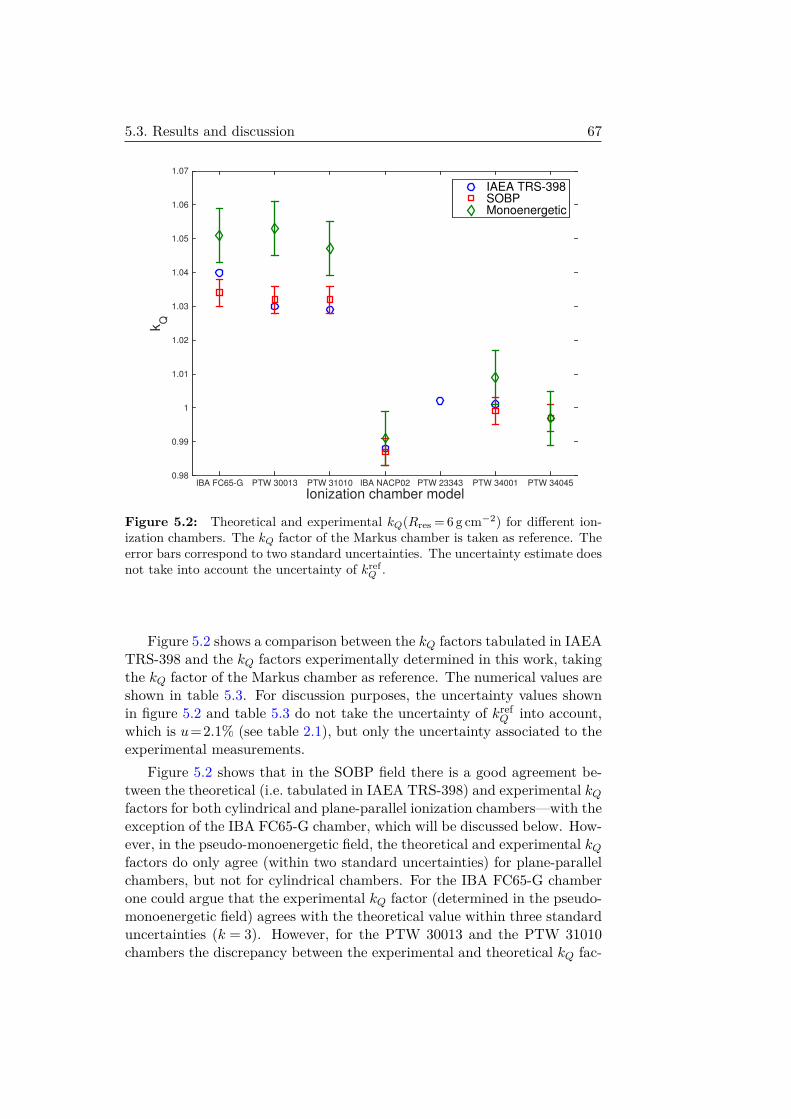
5.3. Results and discussion 67
Ionization chamber modelIBA FC65-G PTW 30013 PTW 31010 IBA NACP02 PTW 23343 PTW 34001 PTW 34045
kQ
0.98
0.99
1
1.01
1.02
1.03
1.04
1.05
1.06
1.07
IAEA TRS-398SOBPMonoenergetic
Figure 5.2: Theoretical and experimental kQ(Rres = 6 g cm−2) for different ion-ization chambers. The kQ factor of the Markus chamber is taken as reference. Theerror bars correspond to two standard uncertainties. The uncertainty estimate doesnot take into account the uncertainty of kref
Q .
Figure 5.2 shows a comparison between the kQ factors tabulated in IAEATRS-398 and the kQ factors experimentally determined in this work, takingthe kQ factor of the Markus chamber as reference. The numerical values areshown in table 5.3. For discussion purposes, the uncertainty values shownin figure 5.2 and table 5.3 do not take the uncertainty of kref
Q into account,which is u=2.1% (see table 2.1), but only the uncertainty associated to theexperimental measurements.
Figure 5.2 shows that in the SOBP field there is a good agreement be-tween the theoretical (i.e. tabulated in IAEA TRS-398) and experimental kQfactors for both cylindrical and plane-parallel ionization chambers—with theexception of the IBA FC65-G chamber, which will be discussed below. How-ever, in the pseudo-monoenergetic field, the theoretical and experimental kQfactors do only agree (within two standard uncertainties) for plane-parallelchambers, but not for cylindrical chambers. For the IBA FC65-G chamberone could argue that the experimental kQ factor (determined in the pseudo-monoenergetic field) agrees with the theoretical value within three standarduncertainties (k = 3). However, for the PTW 30013 and the PTW 31010chambers the discrepancy between the experimental and theoretical kQ fac-

68 Chapter 5. Experimental validation of kQ factors
tors cannot be explained by these means. Note from equation (5.1) thata higher kQ factor may be explained by a lower reading of the chamber inthe user beam quality (MQ). Therefore, the higher kQ factors obtained forcylindrical ionization chambers in pseudo-monoenergetic proton beam fieldscould be explained by the fact that, under these reference conditions, thereading of cylindrical ionization chambers is lower than it should. Theseresults agree with the findings of chapter 4, where we pointed out that, forcylindrical ionization chambers in pseudo-monoenergetic fields, the IAEATRS-398 recommendation of positioning the reference point of the cham-ber at the reference depth leads to a systematic underestimation of Dw,especially relevant for low Rres. Thus, the results of this chapter supportthe suggestion that, for pseudo-monoenergetic proton beams, the effectivepoint of measurement (Peff) of cylindrical ionization chambers should bepositioned at the reference depth. Or, alternatively, dose gradient effectsshould be corrected when using cylindrical ionization chambers (Palmanset al. 2001). Note that, for plane-parallel ionization chambers, the referencepoint of the chamber is already defined to be at Peff (see table 2.2).
In SOBP fields, where dose gradients are small, the effect of Peff in cylin-drical ionization chambers is minor. In this case figure 5.2 also shows that,when taking the kQ factor of the Markus chamber as reference, the experi-mental kQ factors of all the ionization chambers (except for the IBA FC65-G) agree with the theoretical values tabulated in IAEA TRS-398 within twostandard uncertainties. In other words, we found that the tabulated valuesof all chambers, except for the IBA FC65-G, are consistent with each other.For the IBA FC65-G, we found that the experimental kQ factor is lower thanthe theoretical one by 0.6%. This result agrees with the results of Palmanset al. (2001) and chapter 4. Using equation (5.2), it can be shown that theratio of kQ factors IBA FC65-G/PTW 30013 determined by Palmans et al.(2001) agrees with the result of this work within 0.1%. In chapter 4 weused an IBA FC65-G and a PTW 31010 chambers (i.e. the same ionizationchamber models than in this chapter, but different serial numbers) simulta-neously calibrated at the same PSDL (METAS) and we obtained Dw valueswith the IBA FC65-G chamber that were approximately 1% lower than theones obtained with the PTW 31010. Thus, the results of this chapter seemto indicate that (at least part of) the discrepancy between the IBA FC65-Gand the PTW 31010 chambers observed in chapter 4 could be due to thefact that the tabulated kQ factor of the IBA FC65-G Farmer is not con-sistent with the tabulated kQ factor of the PTW 31010 Semiflex (and therest of ionization chamber models studied here). Nonetheless, it should bementioned that a discrepancy of 0.6% is well within the uncertainty of thekQ factors estimated in IAEA TRS-398 (see table 2.1).

5.4. Conclusions 69
5.4 ConclusionsIn this chapter we presented a method to experimentally validate the kQfactors tabulated in IAEA TRS-398 for proton beams and to determine thekQ factors of non-tabulated ionization chambers, based on the already ex-isting ones. We found that the tabulated kQ factors of all the ionizationchambers studied (except for the IBA FC65-G) are consistent with eachother; whereas the tabulated kQ factor of the IBA FC65-G is not consis-tent with the rest—the experimental value being 0.6% lower than the tab-ulated one. For the PTW 34045 Advanced Markus chamber, we found thatkQ(Rres = 6 g cm−2) = 0.997(21) (k = 1), based on the tabulated value ofthe PTW Markus chamber. Finally, concerning the reference dosimetry ofpseudo-monoenergetic proton beams, this chapter provides arguments—inaddition to the ones given by Palmans et al. (2001) and in chapter 4—infavour of positioning the effective point of measurement of cylindrical ion-ization chambers at the reference depth.

70 Chapter 5. Experimental validation of kQ factors

Chapter 6
Monte Carlo calculation ofbeam quality correctionfactors for proton beams
This chapter is based on Gomà et al. (2016). It describes the calculation ofbeam quality correction factors in monoenergetic proton beams, based onthe Monte Carlo simulation of ionization chambers. It uses the Monte Carlocode penh and electronic stopping powers resulting from the adoption of twodifferent sets of mean excitation energy values for water and graphite: (i) thecurrently ICRU recommended Iw =75 eV and Ig =78 eV and (ii) the recentlyproposed Iw = 78 eV and Ig = 81.1 eV. Twelve different ionization chambermodels were studied. The Monte Carlo calculated kQ factors obtained inthis chapter were compared to the experimental data obtained in chapters 4and 5, as well as to other experimental data published in the literature.
6.1 Introduction
As discussed in section 1.2, due to a lack of an appropriate Monte Carlo code,no Monte Carlo calculations of beam quality correction factors in protonbeams have been done so far using the approach of Sempau et al. (2004),i.e. using equation (2.47). Recently Salvat (2013) has developed penh, anextension of the penelope code that includes the transport of protons basedon their electromagnetic interactions in matter. Proton nuclear interactions,however, have not been included. Sterpin et al. (2013) introduced protonnuclear interactions for six isotopes (1H, 12C, 14N, 16O, 31P, 40Ca) in penh.However, the simulation of ionization chambers requires more than these sixisotopes. Although not dominant, the effect of proton nuclear interactionscannot be neglected in proton therapy. Whereas the contribution of chargedparticles heavier than protons to the absorbed dose to water might, ona first approximation, be considered negligible (Paganetti 2002, Fippel &
71

72 Chapter 6. Monte Carlo calculation of kQ factors
Soukup 2004), the contribution of secondary protons (i.e. protons originatingfrom inelastic nuclear interactions) cannot be disregarded, as they contributeroughly to 10% of the dose deposited by a proton beam in the clinical energyrange (Paganetti 2002).
This chapter describes the calculation of beam quality correction factorsfor monoenergetic proton beams. The calculation is based on a detailedMonte Carlo simulation of ionization chambers in proton and 60Co gammaradiation beams, and the use of equation (2.47). kQ,Q0 factors were calcu-lated for a wide range of plane-parallel ionization chambers and a limitedset of cylindrical ionization chambers. Two different sets of mean exitationenergy values for water (Iw) and graphite (Ig) were used: (i) the ICRU 37and ICRU 49 values currently in use (Iw =75 eV and Ig =78 eV); and (ii) thelatest I-values for water (Iw = 78 eV, Andreo et al. (2013)) and graphite(Ig = 81.1 eV, Burns et al. (2014)), to be recommended in a forthcomingICRU report on key data for ionizing radiation dosimetry. Two differentWair values for proton beams were also used accordingly (Andreo et al.2013).
6.2 Materials and methodsWe took 60Co gamma radiation as the reference beam quality Q0 and mo-noenergetic proton beams of energies from 70 to 250 MeV as the user beamquality Q.
This section describes: (i) the Monte Carlo codes used in this chap-ter, (ii) the reference conditions used and the geometry of the simulations,(iii) the radiation sources, (iv) the transport simulation parameters, (v) thegeometry of the simulated ionization chambers, and (vi) the Wair,Q valuesused.
6.2.1 Monte Carlo simulation codes
We used penh (Salvat 2013) for the calculation of beam quality correc-tion factors in proton beams. penh is a Fortran subroutine package, whichis linked to penelope (Salvat 2014), thus allowing for the simulation ofcoupled proton-electron-photon transport processes. As main program weused a version of penEasy (Sempau et al. 2011) that includes penh. Asmentioned above, the only drawback of penh is that it does not includeproton nuclear interactions and, therefore, it does not include the transportof secondary protons originating from inelastic nuclear interactions.
As the influence of secondary protons cannot be disregarded, we also usedGamos to generate a realistic phase-space file (PSF) in water, just in front ofthe ionization chamber (see below). More specifically, we used Gamosv4.1.0,which runs on Geantv4.9.6p02. We used the QGSP_BIC_EMY physicslist (see section 3.2), together with the options: (i) G4EmPenelopePhysics

6.2. Materials and methods 73
for the electromagnetic processes of photons, electrons and positrons, and(ii) G4UrbanMscModel96 for the multiple Coulomb scattering of electrons.
6.2.2 Reference conditions and geometry of the simulations
For the reference beam quality 60Co we followed the reference conditionsdescribed in IAEA TRS-398. That is, we defined a 20× 20× 15 cm3 waterphantom and we set the reference depth (zref) to 5 g cm−2, the source-to-chamber distance (SCD) to 100 cm and the field size at the reference depthto 10× 10 cm2. For proton beams we also followed the reference conditionsfor monoenergetic proton beams described in IAEA TRS-398, but we set thereference depth to 2 g cm−2, instead of 3 g cm−2, as extensively discussedin chapter 4. To speed up the simulations of proton beams we used a waterphantom of 20 × 20 × 5 cm3, since proton backscatter can be considerednegligible—see e.g. Salvat (2013).
The absorbed dose to water at the reference depth was calculated as theaverage absorbed dose to water scored in a disc of 1 cm of radius and 250 µmof thickness centered at zref . This procedure introduced by Sempau et al.(2004) has become a common method to compute Dw in fQ calculations,where the absorbed dose to water in a point is approximated by the averageabsorbed dose to water scored in a small volume. Dair was calculated asthe average absorbed dose to air in the ionization chamber sensitive volume.For both 60Co and proton beams the ionization chambers were positionedas described in IAEA TRS-398, i.e. the reference point of the chamber waspositioned on the central axis of the beam at the reference depth. For cylin-drical chambers the reference point of the chamber is the center of the cavityvolume; for plane-parallel chambers, it is on the inner surface of the entrancewindow at its center (see table 2.2). Chapters 4 and 5 questioned the IAEATRS-398 recommendation of setting the reference point of cylindrical cham-bers at the reference depth for monoenergetic proton beams. This point willnot be addressed in this chapter. Herein we focused on the calculation ofkQ for plane-parallel chambers, which are not affected by this debate. Wealso simulated a limited set of cylindrical chambers, in order to validate oursimulations with published experimental data.
6.2.3 Radiation sources
As 60Co-beam source we simulated a photon point source located 100 cmaway from zref , shaping a 10×10 cm2 field at zref . The energy of the photonsemerging from the source was sampled from the spectrum of the BureauInternational des Poids et Mesures (BIPM) 60Co-source published by Burns(2003). As this spectrum had been scored at a distance of 90 cm from thesource, we transported the photons through 90 cm of vacuum and 5 cm ofair before reaching the water phantom.

74 Chapter 6. Monte Carlo calculation of kQ factors
Table 6.1: Equivalence between proton energy and range in water for differentIw-values. All range values (RCSDA, Rp and Rres) are expressed in g cm−2.
Iw = 75 eVE (MeV) 70 100 150 200 250RCSDA 4.08 7.72 15.77 25.96 37.94Rp 4.15 7.85 16.03 26.37 38.52Rres (zref =2 g cm−2) 2.15 5.85 14.03 24.37 36.52
Iw = 78 eVE (MeV) 70 100 150 200 250RCSDA 4.10 7.76 15.86 26.09 38.01Rp 4.18 7.89 16.12 26.51 38.72Rres (zref =2 g cm−2) 2.18 5.89 14.12 24.51 36.72
As proton source we used a phase-space file generated with Gamos. Wesimulated a planar 10 × 10 cm2 proton beam impinging on the surface of awater phantom. The incident protons were monoenergetic, monodirectionaland perpendicular to the water phantom surface. We scored a PSF at thedepth of 15 mm in water, including only those particles that penh can trans-port, i.e. protons, electrons, positrons and photons. PSFs were generatedfor five different proton energies (70, 100, 150, 200 and 250 MeV) and theywere subsequently used as input PSF sources in penh. Table 6.1 shows theequivalence between the initial energy of the proton beam and the range inwater for different Iw-values. The continuous slowing down approximationrange (RCSDA), the practical range (Rp) and the residual range (Rres) aredefined in 2.2. In table 6.1 the residual range is given for a reference depthof zref =2 g cm−2.
It is important to point out that, in the calculation of the beam qual-ity correction factors, we assumed that the contribution to Dw from thesecondary protons and heavier charged particles generated in the vicinityof the reference point of measurement is comparable to the contribution toDair from the secondary protons and heavier charged particles generated inthe ionization chamber materials. Thus, this work assumes that these twocontributions cancel out in the numerator of equation (2.47) and thereforehave a negligible effect on the calculated kQ values. This assumption is, ofcourse, an additional source of uncertainty in the final kQ factors.

6.2. Materials and methods 75
6.2.4 Transport simulation parameters
GAMOS
In Gamos we set the production cuts for photons, electrons and positrons to2.5 µm and the absorption energies of photons to Eabs(γ)=1 keV, electronsand positrons to Eabs(e−) = Eabs(e+) = 200 keV and protons to Eabs(p) =1 MeV. Finally we limited the maximum step size of charged particles, sothat they interacted at least 20 times before reaching the PSF scoring plane.
PENH
The transport simulation parameters in penh are the same as in penelopeand they are described in detail in Salvat (2014).
In this work all the simulations had the same structure: a scoring vol-ume, a detailed simulation region (around the scoring volume) and a mixed(class II) simulation region (surrounding these two). The scoring volumewas either the water cavity (assumed to be good representative of a point)or the ionization chamber sensitive volume. The detailed and mixed simu-lation volumes were defined arbitrarily, but conservatively, as follows. Wetransported all electrons with energy higher than 200 keV, as these electronshave a radiation yield in water larger than 0.1%. Where the probability fora 200 keV electron of reaching the scoring volume was negligible, we set theabsorption energy for electrons to Eabs(e−) = 200 keV; where it was non-negligible, we set it to Eabs(e−) = 1 keV. In water, for instance, we definedthis probability based on the RCSDA in water of a 200 keV electron, multi-plied by a factor of 1.2—to account for the possibility that an electon maytravel a distance beyond its RCSDA due to energy-loss straggling (Sempau& Andreo 2006). In ionization chamber geometries the influence of the dif-ferent materials was taken into account. Finally, we defined the detailedand mixed simulation volumes as the regions with Eabs(e−) = 1 keV andEabs(e−)=200 keV, respectively.
Absorption energies for photons and protons were set to Eabs(γ)=1 keVand Eabs(p)=1 MeV for all regions. In the scoring volume and the detailedsimulation region we used detailed simulation, i.e. we simulated every singleinteraction. Absorption energies for electrons and positrons were set toEabs(e−) = Eabs(e+) = 1 keV and all the transport simulation parameters(C1, C2, Wcc, and Wcr) for all charged particles were set to zero. In themixed simulation region the absorption energy for electrons and positronswas 200 keV. For all charged particles we used Wcc =10 keV and Wcr =1 keVand we increased gradually C1 and C2 from 0.05 (everywhere in the mixedsimulation region within a distance less than or equal to 5 mm from thescoring volume) to 0.1 (elsewhere). In the mixed simulation region we alsoset dsmax in such a way that each charged particle interacted at least 20times in each body.

76 Chapter 6. Monte Carlo calculation of kQ factors
Table 6.2: Dimensions and material composition of the plane-parallel ionizationchambers simulated in this work.
Ionization Entrance Electrode Collecting Sensitive Guardchamber window spacing electrode volume ringmodel thickness thickness radius width
ExradinA10 0.99 mm PMMA 2.01 mm 0.38 mm C552 2.85 mm 4.1 mm
0.10 mm air25 µm kapton
A11 0.99 mm C552 2.01 mm 0.51 mm C552 9.93 mm 4.4 mmA11TW 0.99 mm PMMA 3 mm 0.51 mm C552 9.93 mm 2.8–4.4 mm
0.10 mm air25 µm kapton
IBANACP-02 0.1 mm mylar 2 mm 50 µm graphite 5 mm 3.25 mm
0.5 mm graphite (ρg = 0.93 g cm−3)(ρg = 1.82 g cm−3) 0.25 mm rexolite
PPC-05 1 mm C552 0.6 mm 0.1 mm graphite 4.95 mm 3.95 mm(ρg = 1.7 g cm−3)0.5 mm PEEK
PPC-40 0.9 mm PMMA 2 mm 0.1 mm graphite 8 mm 4.0 mm0.1 mm graphite (ρg = 0.93 g cm−3)(ρg = 0.93 g cm−3)
PTWAdvanced 0.87 mm PMMA 1 mm 20 µm graphite 2.5 mm 2 mmMarkus 0.4 mm air (ρg = 0.82 g cm−3)
30 µm polyethyleneMarkus 0.87 mm PMMA 2 mm 20 µm graphite 2.65 mm 0.25 mm
0.4 mm air (ρg = 0.82 g cm−3)30 µm polyethylene
Roos 1.1 mm PMMA 2 mm 20 µm graphite 7.5 mm 4 mm20 µm graphite (ρg = 0.82 g cm−3)(ρg = 0.82 g cm−3)
To reduce the statistical uncertainty, we also applied the variance reduc-tion technique of particle splitting to all the particles reaching the scoringvolume (with a splitting factor of 10). We implemented particle splitting insuch a way that split particles could not be split again.
6.2.5 Ionization chambers
As mentioned above, this work focuses on the simulation of plane-parallelionization chambers. We simulated accurately the geometry of nine differentchambers: the Exradin A10, A11 and A11TW (Standard Imaging, Middle-ton WI, USA); the IBA NACP-02, PPC-05 and PPC-40; and the PTW Ad-vanced Markus (Type 34045), Markus (Type 23343) and Roos (Type 34001).For the Exradin and IBA plane-parallel chambers very detailed descriptionsof the geometry and materials of the chambers were provided by the man-ufacturers. For the Exradin chambers geometry files were built from theblueprints; for the IBA chambers we adapted the geometry files prepared by

6.3. Results and discussion 77
Sempau et al. (2004). For the PTW chambers a less detailed description ofthe geometry and partial information of the materials of the chambers werealso provided by the manufacturer. It is well-known that small variationsin the dimensions and material composition of the detection volume andsurrounding bodies (entrance window, collecting electrode, guard ring, etc.)have a significant effect on Dair. Table 6.2 summarizes the dimensions andmaterial composition of the plane-parallel ionization chambers simulated inthis work.
In addition to plane-parallel chambers, we also simulated three differentmodels of cylindrical chambers: IBA FC65-G, IBA FC65-P and NE 2571.As mentioned above, we simulated this limited set of cylindrical chambersin order to validate our calculations with the few experimental data avail-able in the literature (Palmans et al. 2001, 2002, Medin et al. 2006, Medin2010) and the results of chapters 4 and 5. The geometry and materials ofthese chambers were taken from manufacturer information (drawings andtechnical specifications) available online. For the NE 2571 we simulated thegeometry using the description and materials of Nuclear Enterprises (1984)and additional information taken from Aird & Farmer (1972) and Wulff et al.(2008). Based on Nuclear Enterprises (1984), we assumed the insulator ma-terial to be polychlorotrifluoroethylene (PCTFE), instead of polytetraflu-oroethylene (PTFE) assumed by other authors (Wulff et al. 2008, Erazo& Lallena 2013). Also, as the NE 2571 is non-waterproof, we simulated a0.5 mm PMMA sleeve around the chamber.
6.2.6 Wair value for proton beams
As pointed out by Andreo et al. (2013)—where new Iw and Ig values werepresented along with their impact on air kerma and absorbed dose to wa-ter standards—for proton beam dosimetry a change in I-values may alsorequire a change in Wair,Q. In this work, in order to calculate the beamquality correction factors for proton beams using equation (2.47), we areinterested in the ratio between Wair,Q and Wair,Q0 . When using ICRU 37and ICRU 49 I-values, we used the currently recommended Wair values(Wair,Q0 = 33.97 eV, Wair,Q = 34.23 eV) (Andreo et al. 2000, Jones et al.2007), so that Wair,Q/Wair,Q0 =1.008(4). According to Andreo et al. (2013),the adoption of Iw =78 eV and Ig =81.1 eV should be accompanied with anincrease in Wair,Q of about 0.6% (i.e. Wair,Q=34.44 eV), under the assump-tion of no changes in pQ, while Wair,Q0 remains unchanged. Thus, whenusing these new I-values, we used Wair,Q/Wair,Q0 =1.014(4).

78 Chapter 6. Monte Carlo calculation of kQ factors
Table 6.3: Monte Carlo calculated fQ0 factors (i.e. for 60Co gamma radiation)for different plane-parallel ionization chambers and comparison with values in theliterature. The values within parenthesis correspond to one standard uncertaintyin the last digits.
Ionization This work Panettieri Muir Zink and Erazochamber Iw =78 eV Iw =75 eV et al. et al. Wulff et al.model Ig =81.1 eV Ig =78 eV (2008) (2012) (2012) (2014)
ExradinA10 1.1225(20) 1.1249(20) 1.0951(5) 1.1088(26)A11 1.1071(15) 1.1087(15) 1.1158(5) 1.1124(16)A11TW 1.0979(14) 1.1016(14) 1.1055(16)IBANACP-02 1.1523(15) 1.1536(15) 1.1578(7) 1.1562(4) 1.1616(5) 1.1509(18)PPC-05 1.1374(18) 1.1381(18) 1.1410(10) 1.1475(5)PPC-40 1.1403(12) 1.1468(12) 1.1455(7) 1.1440(5)PTWAdv. Markus 1.1470(23) 1.1464(23) 1.1446(5) 1.1478(6)Markus 1.1434(18) 1.1456(18) 1.1416(4) 1.1467(7)Roos 1.1406(12) 1.1459(12) 1.1485(5) 1.1509(5)
Table 6.4: Monte Carlo calculated fQ0 factors (i.e. for 60Co gamma radiation) forcylindrical ionization chambers and comparison with values in the literature. Thevalues within parenthesis correspond to one standard uncertainty in the last digit.
Iw =75 eV; Ig =78 eV Iw =78 eV; Ig =81.1 eV
Ionization This Muir and Andreo This Andreochamber work Rogers et al. work et al.model (2010) (2013) (2013)
IBA FC65-G 1.1123(9) 1.1134(5) 1.1050(9)IBA FC65-P 1.1169(9) 1.1134(5) 1.1145(9)NE 2571 1.1111(9) 1.1124(4) 1.114(1) 1.1039(9) 1.110(1)
6.3 Results and discussion
6.3.1 60Co beam quality
Table 6.3 and table 6.4 show the Monte Carlo calculated fQ0 factors (i.e. for60Co gamma radiation) for the different plane-parallel and cylindrical ion-ization chambers studied in this work. We calculated the fQ0 factors usingthe electronic stopping powers resulting from the adoption of two differ-ent sets of I-values for water and graphite: the ICRU I-values (Iw = 75 eV;Ig =78 eV) and the new I-values proposed by Andreo et al. (2013) and Burnset al. (2014) (Iw =78 eV; Ig =81.1 eV).
Table 6.3 also shows other fQ0 factors published in the literature for thesame plane-parallel ionization chambers and calculated using the ICRU I-values. Panettieri et al. (2008) calculated the fQ0 factor for the three IBA

6.3. Results and discussion 79
plane-parallel chambers studied in this work with penelope-2006. Theauthors used three different 60Co sources (a monoenergetic beam, a photonspectrum and a phase-space file). The values shown in table 6.3 are the fQ0
factors reported as the weighted mean of the values obtained with the threedifferent 60Co sources.
Muir et al. (2012) calculated kQ factors in megavoltage photon beamsfor most of the ionization chambers studied in this work with egsnrc. Al-though the explicit fQ0 factors were not reported in their work, the values intable 6.3 were provided by the authors in a private communication. For theNACP-02 fQ0 factor, table 6.3 shows the value corresponding to the geome-try studied in this work (0.6 mm-thick entrance window, ρg = 1.82 g cm−3),also provided by the authors.
Zink & Wulff (2012) calculated the perturbarion correction factors pQ0
for the NACP-02 and the three PTW chambers studied in this work withegsnrc. The values shown in table 6.3 are the product of the reportedpQ0 factors and the IAEA TRS-398 water/air stopping power ratio for 60Cogamma radiation, sw,air,Q0 = 1.133. The uncertainty values shown in ta-ble 6.3 correspond to the uncertainty estimates given by these authors forthe pQ0 factors—i.e. they do not take the uncertainty of sw,air,Q0 into ac-count. Again, for the NACP-02 fQ0 factor we took the value correspondingto the geometry studied in this work.
Finally Erazo et al. (2014) calculated kQ,Q0 factors for electron beamsfor the NACP-02 and the three Exradin ionization chambers studied inthis work with penelope-2011. Although the explicit fQ0 factors were notreported in their work, the values in table 6.3 were also provided by theauthors in a private communication.
Table 6.4 also shows fQ0 factors for cylindrical chambers published inthe literature. Muir & Rogers (2010) calculated kQ factors in megavoltagephoton beams for the three cylindrical chambers studied in this work withegsnrc and using ICRU I-values. Although the explicit fQ0 factors were notreported in their work, the values in table 6.4 were provided by the authorsin a private communication. Andreo et al. (2013) calculated the fQ0 factorof the NE 2571 for the same two sets of I-values studied in this work, alsowith egsnrc.
For the plane-parallel ionization chambers studied in this work we foundthat the adoption of new I-values leads to a decrease in fQ0 of around 0.2%,ranging from no changes (PTW Adv. Markus) to a decrease of about 0.6%(IBA PPC-40). It should be noticed that the estimate of Andreo et al. (2013)for the decrease in sw,air,Q0 (resulting from the adoption of new I-values)was 0.6%. Hence, the new I-values cause an increase in the perturbationcorrection factors for 60Co estimated to be negligible for the IBA PPC-40chamber and up to 0.6% for the PTW Adv. Markus, where the changes insw,air,Q0 and pQ0 practically cancel each other.
For cylindrical chambers the adoption of new I-values results in a de-

80 Chapter 6. Monte Carlo calculation of kQ factors
crease in fQ0 of 0.2% for the IBA FC65-P and of about 0.7% for the graphite-walled chambers (IBA FC65-G and NE 2571). Thus, for graphite-walledcylindrical chambers, the new I-values result in negligible changes in pQ0 ,which is consistent with the 0.2% increase estimated by Andreo et al. (2013)for the NE 2571.
The vast majority of fQ0 factors calculated in this work using ICRUI-values agree with those published in the literature calculated, using thesame I-values, within 0.5%—which are differences consistent with the useof different Monte Carlo codes. In what follows, we will limit the discussionof the results to those differences larger than 0.5%.
For the Exradin A10 our fQ0 factor differs by 1.5% and 2.7% from thevalues of Erazo et al. (2014) and Muir et al. (2012), respectively. Such largedifferences are only observed with this ionization chamber model. In addi-tion to the Monte Carlo code (or its version) and the 60Co spectrum used,there are two important differences between our simulations and those bythese authors: (i) for the description of the geometry we used an updatedversion of the A10 blueprints provided by the manufacturer, fixing a ‘bug’in the vicinity of the chamber sensitive volume; and (ii) the transport sim-ulation parameters used in the chamber sensitive volume and surroundingbodies were rather different. Whereas our work used detailed simulation(i.e. all collisions were simulated), these authors used a mixed simulationscheme. The smaller the air cavity, the larger the influence of transportsimulation parameters. This explains the larger effect on the A10 chamber,which has a small sensitive volume (see table 6.2).
The fQ0 factor of the NACP-02 chamber agrees within 0.2%, 0.2% and0.4% with the values of Muir et al. (2012), Erazo et al. (2014) and Panettieriet al. (2008), respectively, but differs by 0.7% from the value of Zink &Wulff (2012). This discrepancy could be explained in terms of the differentmaterial composition of the collecting electrode used by Zink &Wulff (2012),which may affect fQ0 by up to 0.5% (Muir et al. 2012).
For the IBA PPC-05 our fQ0 factor agrees within 0.3% with the value ofPanettieri et al. (2008), but it differs by 0.8% from the value of Muir et al.(2012). As in the case of the Exradin A10 chamber, this discrepancy couldarise from the difference between detailed and mixed simulation—which, asmentioned above, is more notorious for small volume ionization chamberslike the IBA PPC-05 (see table 6.2).
6.3.2 Proton beam qualities
Table 6.5 shows the Monte Carlo calculated beam quality correction factorsin monoenergetic proton beams for all the ionization chambers studied inthis work, at a reference depth of 2 g cm−2, as a function of the initial energyof the beam. The uncertainty estimate shown is the combined standarduncertainty of fQ (type A), fQ0 (type A) and Wair,Q/Wair,Q0 (type B). Note

6.3. Results and discussion 81
Table 6.5: Monte Carlo calculated kQ factors for monoenergetic proton beams,at the reference depth of 2 g cm−2, as a function of the initial proton energy. Thevalues within parenthesis correspond to one standard uncertainty in the last digit.
Iw =75 eV; Ig =78 eV; Wair,Q/Wair,Q0 =1.008E (MeV)
IC model 70 100 150 200 250
ExradinA10 1.012(6) 1.019(6) 1.007(6) 1.020(6) 1.013(6)A11 1.012(6) 1.023(5) 1.022(5) 1.025(5) 1.022(6)A11TW 1.031(6) 1.030(5) 1.030(5) 1.032(5) 1.029(6)IBANACP-02 0.983(5) 0.988(5) 0.987(5) 0.986(5) 0.990(5)PPC-05 0.994(5) 1.003(5) 0.999(5) 1.001(5) 1.004(6)PPC-40 0.991(5) 0.991(5) 0.992(5) 0.993(5) 0.991(5)PTWAdv. Markus 1.007(6) 1.002(6) 0.991(6) 1.000(7) 0.995(7)Markus 1.004(6) 1.006(6) 1.000(6) 0.999(6) 0.992(6)Roos 0.992(5) 0.993(5) 0.993(5) 0.995(5) 0.994(5)
IBAFC65-G 1.065(5) 1.036(5) 1.022(5) 1.021(5) 1.021(5)FC65-P 1.066(5) 1.037(5) 1.022(5) 1.022(5) 1.019(5)NE2571 1.064(5) 1.037(5) 1.022(5) 1.022(5) 1.024(5)
Iw =78 eV; Ig =81.1 eV; Wair,Q/Wair,Q0 =1.014E (MeV)
IC model 70 100 150 200 250
ExradinA10 1.013(6) 1.013(6) 1.023(6) 1.021(6) 1.021(6)A11 1.014(5) 1.026(5) 1.023(5) 1.025(5) 1.028(6)A11TW 1.034(6) 1.039(5) 1.038(5) 1.034(5) 1.038(6)IBANACP-02 0.981(5) 0.987(5) 0.987(5) 0.988(5) 0.989(5)PPC-05 0.990(5) 1.003(5) 1.007(5) 1.003(5) 1.004(6)PPC-40 0.992(5) 0.996(5) 0.998(5) 0.996(5) 0.997(5)PTWAdv. Markus 1.001(6) 0.997(6) 1.003(6) 1.002(7) 1.006(7)Markus 1.002(6) 1.002(6) 1.012(6) 1.008(6) 1.007(6)Roos 0.993(5) 0.994(5) 0.998(5) 0.999(5) 0.999(5)
IBAFC65-G 1.067(5) 1.040(5) 1.031(5) 1.025(5) 1.020(5)FC65-P 1.065(5) 1.039(5) 1.029(5) 1.025(5) 1.022(5)NE2571 1.069(5) 1.043(5) 1.032(5) 1.027(5) 1.023(5)

82 Chapter 6. Monte Carlo calculation of kQ factors
Rres
(g cm-2
)
0 5 10 15 20 25 30 35 40
kQ
1
1.01
1.02
1.03
1.04
1.05
1.06
1.07
1.08IBA FC65-G
IAEA TRS-398This work (I
w = 75 eV; I
g = 78 eV)
This work (Iw
= 78 eV; Ig = 81.1 eV)
Medin et al (2006)
(a)
Rres
(g cm-2
)
0 5 10 15 20 25 30 35 40
kQ
1
1.01
1.02
1.03
1.04
1.05
1.06
1.07
1.08NE 2571
IAEA TRS-398This work (I
w = 75 eV; I
g = 78 eV)
This work (Iw
= 78 eV; Ig = 81.1 eV)
Medin et al (2006)Medin (2010)
(b)
Figure 6.1: Comparison of the Monte Carlo kQ factors for cylindrical ionizationchambers calculated in this work and the IAEA TRS-398 kQ factors (solid line),calculated using ICRU I-values, as a function of Rres. The uncertainty bars andthe dashed lines correspond to one standard uncertainty in the data points and theIAEA TRS-398 values, respectively.

6.3. Results and discussion 83
Rres
(g cm-2
)
0 5 10 15 20 25 30 35 40
kQ
0.95
0.96
0.97
0.98
0.99
1
1.01
1.02
1.03IBA NACP-02
IAEA TRS-398This work (I
w = 75 eV; I
g = 78 eV)
This work (Iw
= 78 eV; Ig = 81.1 eV)
(a)R
res (g cm
-2)
0 5 10 15 20 25 30 35 40
kQ
0.96
0.97
0.98
0.99
1
1.01
1.02
1.03
1.04IBA PPC-05
IAEA TRS-398This work (I
w = 75 eV; I
g = 78 eV)
This work (Iw
= 78 eV; Ig = 81.1 eV)
(b)
Rres
(g cm-2
)
0 5 10 15 20 25 30 35 40
kQ
0.96
0.97
0.98
0.99
1
1.01
1.02
1.03
1.04IBA PPC-40
IAEA TRS-398This work (I
w = 75 eV; I
g = 78 eV)
This work (Iw
= 78 eV; Ig = 81.1 eV)
(c)R
res (g cm
-2)
0 5 10 15 20 25 30 35 40
kQ
0.96
0.97
0.98
0.99
1
1.01
1.02
1.03
1.04PTW Markus
IAEA TRS-398This work (I
w = 75 eV; I
g = 78 eV)
This work (Iw
= 78 eV; Ig = 81.1 eV)
(d)
Rres
(g cm-2
)
0 5 10 15 20 25 30 35 40
kQ
0.96
0.97
0.98
0.99
1
1.01
1.02
1.03
1.04PTW Roos
IAEA TRS-398This work (I
w = 75 eV; I
g = 78 eV)
This work (Iw
= 78 eV; Ig = 81.1 eV)
(e)
Figure 6.2: Comparison of the Monte Carlo kQ factors for plane-parallel ion-ization chambers calculated in this work and the IAEA TRS-398 kQ factors (solidline), calculated using ICRU I-values, as a function of Rres. The uncertainty barsand the dashed lines correspond to one standard uncertainty in the data points andthe IAEA TRS-398 values, respectively.
84 Chapter 6. Monte Carlo calculation of kQ factors
that fQ factors may be obtained by simply dividing the kQ factors by theWair ratio and the corresponding fQ0 factor in table 6.3 (or table 6.4).
From the values in table 6.5 it can be seen that the adoption of newI-values results in an average increase in kQ of about 0.3%—changes in kQfactors are, however, strongly dependent on the ionization chamber model.For plane-parallel chambers, changes in kQ range from -0.6% up to 1.6%;for cylindrical chambers, they range from -0.1% to 1%. For the NE 2571we obtained an average increase in kQ of about 0.5%, which agrees withinone standard uncertainty with the estimate of Andreo et al. (2013) of nochanges (based on the assumption of negligible perturbation effects).
Figure 6.1 and figure 6.2 show a comparison between the kQ factorsof some of the ionization chambers studied in this work (calculated withthe two sets of I-values) and the kQ factors tabulated in IAEA TRS-398(calculated using ICRU I-values), as a function of the residual range—seetable 6.1 for energy-range equivalence. Figure 6.1 shows the kQ factors forcylindrical ionization chambers and it includes the experimental values ofMedin et al. (2006) and Medin (2010), determined with water calorimetry.Figure 6.2 shows the kQ factors for plane-parallel chambers.
All the kQ factors calculated in this work using ICRU I-values agreewithin 2.3% or better with the kQ factors tabulated in IAEA TRS-398 andwithin 1% or better with the experimental values of Medin et al. (2006) andMedin (2010). The kQ factors calculated using Iw = 78 eV and Ig = 81.1 eValso agree within 1.1% or better with the experimental values. Despite thisagreement, the dependence of our kQ factors with the residual range showsa different trend than IAEA TRS-398 values.
For cylindrical chambers, figure 6.1 shows that the variation of our kQfactors with the residual range is of the order of 5% (within a Rres rangefrom 2 to 37 g cm−2), much larger than that of IAEA TRS-398 values(smaller than 0.5%). Such a variation is mainly due to the increase of ourkQ factors at small residual ranges, which, in turn, is due to the fact that thereference point of the chamber—and not its effective point of measurement—is positioned at the reference measurement depth, as extensively discussedin chapters 4 and 5.
For plane-parallel ionization chambers, figure 6.2 shows that the agree-ment between our kQ factors and IAEA TRS-398 values is better (almostalways within 1%) than for cylindrical ionization chambers. However, thevariation of the kQ factors with the residual range seems to follow a differenttrend. Whereas IAEA TRS-398 kQ factors decrease slightly with increas-ing residual range, our kQ factors seem to slightly increase with increasingresidual range.
Excluding the case of cylindrical chambers at small residual ranges (be-cause of the reasons mentioned above), all our kQ factors calculated usingICRU I-values agree with the IAEA TRS-398 values within the standarduncertainty stated in the Code of Practice. Compatible with this agreement

6.3. Results and discussion 85
Table 6.6: Ratio of kQ factors, at the reference depth of 2 g cm−2, of differentionization chambers studied in this chapter and comparison with experimental val-ues in the literature. The values within parenthesis correspond to one standarduncertainty in the last digit.
Rres ∼ 2.5 g cm−2
Ionization This work Palmans Palmanschamber Iw =75 eV Iw =78 eV et al. et al.ratio Ig =78 eV Ig =81.1 eV (2001) (2002)
IBA FC65-G/NE 2571 1.001(2) 0.998(2) 0.997(2)IBA NACP-02/NE 2571 0.923(3) 0.917(3) 0.930(3)PTW Markus/NE 2571 0.943(4) 0.938(4) 0.940(3)PTW Roos/NE 2571 0.932(2) 0.929(2) 0.937(3)
Rres (g cm−2) 2.15 2.18 2.65 2.65
Rres ' 6 g cm−2
Ionization This work Chapter 5chamber Iw =75 eV Iw =78 eVratio Ig =78 eV Ig =81.1 eV
IBA NACP-02/IBA FC65-G 0.954(3) 0.948(3) 0.943(4)PTW Adv. Markus/IBA FC65-G 0.967(5) 0.958(5) 0.949(4)PTW Markus/IBA FC65-G 0.971(4) 0.963(4) 0.953(4)PTW Roos/IBA FC65-G 0.958(2) 0.955(2) 0.960(4)
Rres (g cm−2) 5.85 5.89 5.93
is the fact that our mean kQ values and IAEA TRS-398 mean values maydiffer by up to 1.8% for some ionization chamber models. Furthermore,these differences (between mean kQ values) are strongly dependent on theionization chamber model and the proton beam quality. Such a dependenceseems to indicate that perturbation correction factors in proton beams couldbe significantly different from unity, at least for the some of the ionizationchambers studied in this work. For graphite-walled Farmer chambers, forinstance, we found that for Rres > 14 g cm−2 the differences between ourmean kQ values and IAEA TRS-398 values are of about 1.7%. Part of thesedifferences (0.8–0.9%) arise from a higher fQ0 factor (fQ0 = 1.111–1.112)than that in IAEA TRS-398 (fQ0 = 1.102). The remaining part arise froma smaller fQ factor, pointing at pQ ∼ 0.992(2), slighly lower than the valuecalculated by Palmans (2011) (pQ=0.9965). Note that these differences (forgraphite-walled Farmer chambers) bring the comparison between referencedosimetry and Faraday dosimetry in chapter 4 in much better agreement—from 3% to approximately 1.5%.
To further validate the Monte Carlo kQ factors calculated in this work,

86 Chapter 6. Monte Carlo calculation of kQ factors
table 6.6 compares the ratio of kQ factors (kQ/krefQ ) for some of the ion-
ization chambers studied in this work with experimental data published inthe literature. Note that the kQ ratio of two ionization chambers has theadvantage that it does not depend on the adoption of specific Wair values.Palmans et al. (2001) and Palmans et al. (2002) determined experimen-tally the ratio of kQ factors between different ionization chambers and theNE 2571 chamber (as reference chamber), for a non-modulated proton beamof Rres = 2.65 cm. In their work, the authors reported pQ ratios (instead ofkQ ratios), after applying a serie of theoretical corrections to the experi-mental data. Herein, we reverted these corrections, so that table 6.6 showsthe experimental kQ ratios obtained by these authors. Also in chapter 5we determined the ratio of kQ factors for different ionization chambers in aproton beam of Rres ' 6 cm. The values shown in table 6.6 correspond tothe results reported for the pseudo-monoenergetic proton beam. Note thathere the IBA FC65-G is taken as reference chamber, instead of the PTWMarkus. The reason for that is the lower quality of the geometry descriptionof PTW chambers (see section 6.2.5).
The kQ ratios calculated in this work using ICRU I-values were found toagree within 0.4%, 0.7% and 1.9%, or better, with the experimental valuesof Palmans et al. (2001), Palmans et al. (2002) and chapter 5, respectively.The kQ ratios calculated using Iw = 78 eV and Ig = 81.1 eV were found toagree within 0.6%, 1.3% and 1.0%, or better, with the experimental valuesof Palmans et al. (2001), Palmans et al. (2002) and chapter 5, respectively.
It is worth mentioning again that the kQ factors calculated in this chapterare based on the assumption that the contribution to the absorbed dose towater at the reference depth from the secondary protons and heavier chargedparticles generated in the vicinity of zref is comparable to the contribution tothe absorbed dose to air in the ionization chamber sensitive volume from thesecondary protons and heavier charged particles generated in the ionizationchamber materials. Despite this assumption, we found a good agreementbetween our Monte Carlo calculated kQ factors and the experimental datapublished in the literature.
Finally, it is important to point out that the kQ factors calculated in thiswork include inherently a correction for dose gradient effects in monoener-getic proton beams. Therefore, they should not be used in modulated protonbeams, where dose gradients are much smaller.
6.4 Conclusions
This chapter calculated fQ0 factors (in 60Co gamma radiation) and kQ fac-tors in monoenergetic proton beams for a wide range of ionization chambers,based on Monte Carlo simulation. We used the electronic stopping powersresulting from the adoption of two different sets of I-values for water and

6.4. Conclusions 87
graphite: ICRU I-values (Iw =75 eV; Ig =78 eV) and new I-values proposedby Andreo et al. (2013) and Burns et al. (2014) (Iw = 78 eV; Ig = 81.1 eV).The fQ0 factors calculated in this work were in good agreement with bothMonte Carlo calculated and experimental values published in the litera-ture. Except for the case of cylindrical chambers at small residual ranges,our Monte Carlo calculated kQ factors agreed with the values tabulated inIAEA TRS-398 and the experimental values in the literature within theirstated standard uncertainties. The results of this work point at perturbationcorrection factors in proton beams that may differ significantly from unityfor some of the ionization chambers studied. Nevertheless, an independentcalculation of kQ factors in proton beams—by other authors and, ideally,with a different Monte Carlo code—would be of interest for the scientificcommunity in order to validate, or question, the kQ factors reported here.

88 Chapter 6. Monte Carlo calculation of kQ factors

Chapter 7
Reference dosimetry ofproton pencil beams basedon dose-area product: aproof of concept
This chapter describes a novel approach to the reference dosimetry of pro-ton pencil beams based on the concept of dose-area product. The dose-areaproduct is the integral of the absorbed dose to water over the plane per-pendicular to the beam direction. For proton pencil beams, the dose-areaproduct is a quantity easier to determine than the absorbed dose to waterat a point. In this chapter, we compare the reference dosimetry of protonpencil beams based on dose-area product with the standard approach basedon the IAEA TRS-398 Code of Practice.
7.1 Introduction
IAEA TRS-398 recommends the determination of the absorbed dose to wa-ter in the centre of a broad field (10× 10 cm2) with a ‘point-like’ ionizationchamber—see table 2.2. In proton (and heavier charged-particle) pencilbeam delivery systems, a broad field can be delivered by scanning the nar-row pencil beam laterally, i.e. across the plane perpendicular to the beamdirection. This way of producing a broad field has nevertheless one maindrawback: it is very sensitive to delivery errors—in particular, to beam po-sition errors. That is, small errors in beam position during the delivery ofthe field might have a significant effect on Dw at the reference point of mea-surement (i.e. at the centre of the field). A more natural, and more robust,approach to the reference dosimetry of narrow pencil beams is the deter-mination of the dose-area product (DwA) with a large-diameter ionization
89

90 Chapter 7. Reference dosimetry based on dose-area product
chamber. The dose-area product, also called integral dose by Pedroni et al.(2005), is the integral of Dw over the plane perpendicular to the beam direc-tion. That is, instead of determining Dw at the centre of a broad field witha small detector, to determine DwA of a small field with a large detector.These two approaches are reciprocal (Attix 1986) and therefore equivalent,as it will be shown below in section 7.2.
The dose-area product is a dosimetric quantity extensively used in diag-nostic radiology (Alm-Carlsson et al. 2007). In particle therapy, it is typi-cally used to express the integrated depth-dose curve of proton (or heaviercharged-particle) pencil beams (Jones et al. 2007). The use of DwA in thedosimetry of small radiotherapy beams was first proposed by Djouguela et al.(2006) for narrow photon beams and it was later used by Gillin et al. (2010)to calibrate the beam monitor chamber of a spot-scanning proton beam de-livery system. In both cases, the authors cross-calibrated a large-diameterionization chamber against a reference cylindrical ionization chamber in abroad field. Gillin et al. (2010) also seem to assume a constant beam qualitycorrection factor (kQ,Qcross) for all the measured proton beam qualities.
In this chapter, we based on IAEA TRS-398 formalism to investigatethe reference dosimetry of proton pencil beams based on DwA. First, wecalibrated a large-diameter ionization chamber in terms of DwA in a 60Cobeam. Second, we calculated the beam quality correction factor of the large-diameter ionization chamber in proton beams in a similar way as in chap-ter 6. Last, we compared the dose-area product approach to the standard‘broad field–small detector’ approach. The advantage of pencil beam scan-ning delivery systems is that they are capable of delivering a homogeneousbroad field by the superposition of narrow fields, which establishes an an-alytical relationship between the broad and narrow field dosimetry, as itis shown below. Thus, proton (or heavier charged particles) pencil beamscanning delivery systems are the ideal delivery systems to test the novelapproach to reference dosimetry described in this chapter.
7.2 Theory
In this section, we will derive the relationship between (i) the dose-area prod-uct or integrated dose (DwA) of a proton pencil beam of lateral Gaussianshape and (ii) the point dose (Dw) at the centre of a uniform field generatedby the superposition of an infinite number of equally-spaced proton pencilbeams.
To begin with, let us define D(x, y, z) as the absorbed dose to waterat a point (x, y, z) in space delivered by a given radiation field. If the z-axis defines the beam direction, the integrated dose, D(z), is defined as the

7.2. Theory 91
integral of D(x, y, z) over the plane perpendicular to the beam direction
D(z) .=+∞∫−∞
+∞∫−∞
D(x, y, z) dx dy. (7.1)
When the radiation field is a single proton pencil beam of lateral Gaussianshape travelling along z and centered at (x0, y0),
D(x, y, z) = D(x0, y0, z) exp(−(x− x0)2
2σ2x
)exp
(−(y − y0)2
2σ2y
)(7.2)
where D(x0, y0, z) is the dose at the centre of the pencil as a function of z;and σx and σy are the standard deviation of the Gaussian function in thedirections x and y, respectively. σx and σy are also a function of z, but thisdependency is omitted in equation (7.2) for the sake of clarity. In this case,the integrated dose is D(z)=2πσxσyD(x0, y0, z), so equation (7.2) may alsobe expressed, in terms of D(z), as
D(x, y, z) = D(z)2πσxσy
exp(−(x− x0)2
2σ2x
)exp
(−(y − y0)2
2σ2y
). (7.3)
Let us now consider the case of a broad uniform field resulting from thesuperposition of an infinite number of proton pencil beams (7.3) separateda distance δx and δy between them. In this case,
D(x, y, z) =∑k∈Z
∑l∈Z
D(z)2πσxσy
exp(−(x− k δx)2
2σ2x
)exp
(−(y − l δy)2
2σ2y
)(7.4)
where k and l extend over all integer numbers Z. Since the field is uniformby definition, equation (7.4) may be re-written as
D(x, y, z) =D(0, 0, z)
= D(z)2πσxσy
∑k∈Z
exp(−(kδx)2
2σ2x
)∑l∈Z
exp(−(lδy)2
2σ2y
)(7.5)
≡ D(z)2πσxσy
I(x)I(y)
where I(x), and I(y), are defined as
I(x) .=∑k∈Z
exp(−(kδx)2
2σ2x
). (7.6)
Defining sx=σx/δx, equation (7.6) may be re-written as
I(x) =∑k∈Z
exp(− k2
2 s2x
)∼=
+∞∫−∞
exp(− k2
2 s2x
)dk =
√2π sx (7.7)

92 Chapter 7. Reference dosimetry based on dose-area product
where in the second equality we used the Euler-McLaurin formula (Grahamet al. 1990), which (i) for a Gaussian function of sx > 1 and (ii) for theaccuracy needed in radiation therapy reference dosimetry, we can safelyassume to be exact. Thus, substituting I(x) and I(y) in equation 7.5, itfollows that
D(0, 0, z) = D(z)δx δy
. (7.8)
That is, the absorbed dose at the centre of a uniform broad field D(0, 0, z)resulting from the superposition of an infinite number of proton pencil beamsequally-spaced a distance δx and δy between them is equal to the integrateddose of a single pencil beam D(z), divided by the spacing δx and δy betweenadjacent pencil beams. For divergent beams, δx and δy are also a functionof z.
Note that equation (7.8) is a simple consequence of the reciprocity theo-rem (Attix 1986). Thus, it has been shown that, when δx6σx and δy6σy,a broad field generated by the superposition of equally-spaced pencil beamsis sufficiently uniform so that the reciprocity theorem applies.
7.3 Materials and methods
7.3.1 DwA based formalism
Making a parallelism with IAEA TRS-398 formalism based on standards ofabsorbed dose to water (see section 2.2.4), we propose a formalism based onstandards of dose-area product, where the absorbed dose to water integratedover an area A in a beam quality Q, (DwA)Q, in the absence of the ionizationchamber, is given by
(DwA)Q = MQNDA,w,Q0 kQ,Q0 (7.9)
where MQ is the reading of the ionization chamber corrected for all thequantities of influence (except for the beam quality); NDA,w,Q0 is the cali-bration coefficient of the ionization chamber in terms of dose-area productin the reference beam quality Q0; and kQ,Q0 is the beam quality correctionfactor in terms of dose-area product.
The calibration coefficient in terms of dose-area product in the referencebeam quality Q0 is given by
NDA,w,Q0 =(DwA)Q0
MQ0(7.10)
where (DwA)Q0is the absorbed dose to water at the reference depth in-
tegrated over a surface A equal to the sensitive surface of the ionizationchamber in the reference beam quality Q0, and MQ0 is the reading of theionization chamber corrected for all quantities of influence.

7.3. Materials and methods 93
The beam quality correction factor in terms of dose-area product, kQ,Q0 ,corrects for the different response of the ionization chamber in the userbeam quality Q and the calibration beam quality Q0. It is defined as theratio of the ionization chamber calibration coefficients, in terms of dose-areaproduct, at the beam qualities Q and Q0 and it can be calculated usingMonte Carlo methods as
kQ,Q0 = fQ
fQ0
Wair,QWair,Q0
= (DwA/Dair)Q(DwA/Dair)Q0
Wair,QWair,Q0
(7.11)
where f is now an ionization chamber-specific and beam quality-dependentfactor that establishes the proportionality between the absorbed dose towater at the reference measurement depth, in the absence of the detector,integrated over the sensitive surface the ionization chamber (DwA) and theaverage absorbed dose to air in the ionization chamber sensitive volume(Dair).
7.3.2 Large-diameter ionization chamber
In this work we used a PTW 34070 Bragg Peak chamber, a large-diameterplane-parallel ionization chamber. According to manufacturer specifications,the radius of the collecting electrode is 40.8 mm, the guard ring width is1.1 mm and the gap between the collector and the guard ring is 0.2 mm.Based on this information, we assumed the radius of the sensitive volume tobe r=40.9 mm, with an uncertainty of δr=0.1 mm. The nominal thicknessof the entrance window is 3.47 mm, which corresponds to a photon water-equivalent thickness of 4 mm.
7.3.3 Calibration in terms of DwA in a 60Co beam
The Bragg Peak chamber was calibrated in terms of dose-area product inthe 60Co beam at the Swiss Federal Institute of Metrology METAS. To theextent possible, we followed the IAEA TRS-398 reference conditions for 60Cobeams (see table 2.2). That is, we set the reference point of the chamber ata depth of 5 g cm−2 in water and the source-to-chamber distance to 100 cm.The reference point of the Bragg Peak chamber was taken to be the centreof the inner surface of the entrance window, i.e. 3.47 mm below the centre ofthe outer surface of the entrance window. The only exception with respectto the IAEA TRS-398 reference conditions was the field size, which was setto 22 × 22 cm2, in order to guarantee a sufficiently uniform Dw across theentire chamber surface.
To be able to trace the calibration in terms of dose-area product to theMETAS primary standard (water calorimeter), we performed the followingsteps:

94 Chapter 7. Reference dosimetry based on dose-area product
1. With a secondary standard (NE 2571 Farmer chamber), we determinedthe ratio between Dw at the centre of the 22× 22 cm2 field and Dw atthe centre of the 10×10 cm2 reference field. We assumed the variationin the photon beam quality between calibration (22 × 22 cm2) andreference (10 × 10 cm2) conditions to be negligible, but we accountedfor this effect in the uncertainty budget (see table 7.1).
2. With an IBA PFD-3G diode, we measured a two-dimensional Dw-mapof the entire 22 × 22 cm2 field, relative to the field centre. With thisfield map, we determined the ratio between Dw at any point in the22× 22 cm2 field and Dw at the centre of the 22× 22 cm2 field.
With these two measurements, we obtained a two-dimensional map ofthe absolute Dw (because traceable to the primary standard) in the entire22×22 cm2 field. To determine the calibration coefficient of the Bragg Peakchamber in terms of dose-area product (7.10), we integrated Dw over thesensitive surface of the Bragg Peak chamber (A=π r2, where r is the radiusof the sensitive volume of the chamber). Note that r enters directly inNDA,w,Q0 . Thus, the uncertainty of this value has a direct impact on theuncertainty of NDA,w,Q0 .
Finally, it should be mentioned that our calibration is terms of dose-areaproduct assumes a uniform response of the Bragg Peak chamber across theentire sensitive surface. In reality, however, the pressure of water againstthe thin entrance window causes a slight decrease in the distance betweenthe front and collecting electrodes, which is more pronounced in the centralpart of the chamber. This effect was assumed to be negligible, but it wasaccounted for in the uncertainty budget based on information provided bythe manufacturer (see table 7.1).
7.3.4 Monte Carlo calculation of kQ factors
The beam quality correction factor of the PTW Bragg Peak chamber inproton beams was calculated similarly as in chapter 6. In what follows, onlythe differences with respect to chapter 6 are described.
First of all, we calculated the kQ factors based on equation (7.11), i.e. interms of dose-area product. As reference conditions for the reference beamquality 60Co we defined a 40 × 40 × 15 cm3 water phantom and we set thereference depth to 5 g cm−2, the source-to-chamber distance to 100 cm andthe field size at the reference depth to 22 × 22 cm2. For proton beams wedefined a 40 × 40 × 5 cm3 water phantom, we set the reference depth to2 g cm−2 and the field size to 22× 22 cm2.
The DwA at the reference depth was calculated as the average absorbeddose to water scored in a disc of 40.8 mm of radius and 250 µm of thick-ness, centred on the central axis of the beam at the reference depth. Dair

7.4. Results and discussion 95
was calculated as the average absorbed dose to air in the Bragg Peak cham-ber sensitive volume—here assumed to have a sensitive radius according tomanufacturer specifications (r=40.8 mm). For both 60Co and proton beamsthe reference point of the chamber was positioned on the central axis of thebeam at the reference depth.
As 60Co beam source we simulated a monoenergetic 1.25 MeV photonpoint source located 100 cm away from zref (i.e. 95 cm away from the waterphantom surface), shaping a 22 × 22 cm2 field at the reference depth. Asproton source we generated a 22 × 22 cm2 phase-space file at a depth of15 mm in water with Gamos for five different proton energies: 70, 100, 150,200 and 250 MeV.
Finally, we also calculate the kQ factor of the PTW Markus chamber asdescribed in chapter 6, but with a monoenergetic 1.25 MeV photon sourceas reference beam quality.
7.3.5 Experimental determination of DwA of a proton pencilbeam
With the large-diameter ionization chamber, we determined the DwA ofdifferent quasi-monoenergetic proton pencil beams (with energies rangingfrom 70 to 230 MeV, in 10 MeV energy steps) using equation (7.9). Thereference point of the Bragg Peak chamber was set at a reference depthof 2 g cm−2 in water. The kQ factors were interpolated from the valuescalculated with Monte Carlo simulation for 70, 100, 150, 200 and 250 MeVmonoenergetic proton beams. Also in this case the water pressure causes aslight decrease in the distance between the front and collecting electrodes,more pronounced in the central part of the chamber—which is preciselywhere the proton pencil beam impinges. This effect was again assumed tobe negligible, but it was accounted for in the uncertainty budget with arelative standard uncertainty of u=0.12%.
Additionally, we determined DwA for the same quasi-monoenergetic pro-ton energies with a conventional ionization chamber using equation (7.8).That is, we determined Dw at the centre of a 10 × 10 cm2 field with aPTW Markus chamber (previously calibrated in terms of Dw at METAS)as described in chapter 4. The reference point of the chamber was set at areference depth of 2 g cm−2 in water and the broad 10 × 10 cm2 field wasgenerated by the superposition of proton pencil beams equally-spaced by adistance δx=δy=2.5 mm. The kQ factors were interpolated from the valuescalculated with Monte Carlo simulation.
7.4 Results and discussionTable 7.1 shows the comparison between the uncertainty estimates of thecalibration coefficient of the Markus chamber (in terms of absorbed dose to

96 Chapter 7. Reference dosimetry based on dose-area product
Table 7.1: Estimated relative standard uncertainty of all the components enteringin the determination of the calibration coefficients in terms of Dw of a Markuschamber and in terms of DwA of a Bragg Peak chamber in the 60Co beam atMETAS. The combined relative standard uncertainty of the calibration coefficientsis also shown. All values are in %.
NMarkusD,w Nbpc
DA,w
uA uB uA uB
Dcalw,10×10 0.36 0.36
Hcal10×10 0.05 0.11 0.05 0.11
HMarkus10×10 0.02 0.02
MMarkus10×10 0.02- kPT 0.05- kh 0.03- kelec 0.06- ks 0.01- kz 0.07
H2s10×10 0.03 0.02
M2s10×10 0.01 (correlated)
H2s22×22 0.02 0.01
M2s22×22 0.02 (correlated)- kQ22×22,Q10×10 0.12
Hbpc22×22 0.00 0.01
Mbpc22×22 0.16- kPT 0.05- kh 0.03- kelec 0.06- ks 0.01- kz 0.07- kwater pressure 0.14
Abpc 0.28
Total 0.06 0.39 0.17 0.52Combined uC 0.40 0.54

7.4. Results and discussion 97
Table 7.2: Monte Carlo calculated kQ factors of the PTW Bragg Peak chamberin monoenergetic proton beams, at the reference depth of 2 g cm−2, as a functionof the initial proton energy. Iw =75 eV, Ig =78 eV and Wair,Q/Wair,Q0 =1.008. Thevalues within parenthesis correspond to one standard uncertainty in the last digit.
E (MeV) kQ
70 0.990(5)100 0.997(5)150 1.001(5)200 1.002(5)250 1.001(5)
water) and the calibration coefficient of the Bragg Peak chamber (in termsof dose-area product), in the 60Co beam at METAS. The superscripts cal,2s and bpc stand for water calorimeter, secondary standard (NE 2571) andBragg Peak chamber, respectively. The subscripts 10×10 and 22×22 referto the field size in cm2. H is the correction factor for field homogeneity, Mis the reading of the ionization chamber and Abpc is the integration surfaceof the Bragg Peak chamber. For instance, Hcal
10×10 is the correction factorthat accounts for the difference between the average Dw integrated over thesensitive surface of the water calorimeter and the ‘point’ Dw at the centreof the reference 10×10 cm2 field.
Table 7.1 shows that the uncertainty estimate of the calibration coeffi-cient in terms of dose-area product (uC = 0.5%) is slightly larger than theuncertainty of the calibration coefficient in terms of absorbed dose to water(uC = 0.4%). This is mainly due to the uncertainty of the sensitive area ofthe Bragg Peak chamber, where a small uncertainty in the integration ra-dius (δr= 0.1 mm) leads to a relatively large uncertainty in the integrationsurface (uB =0.3%, see table 7.1).
Table 7.2 shows the Monte Carlo calculated kQ factors of the PTW BraggPeak chamber in monoenergetic proton beams, at the reference depth of2 g cm−2, as a function of the initial proton energy. The variation of the kQfactors with the initial energy of the proton beam follows the same trendthan the kQ factors of plane-parallel chambers in table 6.5.
Finally, figure 7.1 shows the comparison between the determination ofDwA (per MU) of a single proton pencil beam with the Bragg Peak chamberusing equation (7.9) and with the Markus chamber using equation (7.8).Note that figure 7.1(a) shows an alternative approach to the calibration ofproton beam monitor chambers to the one described in chapter 4—i.e. thecalibration curve shown in figure 7.1(a) (in terms of DwA/MU) is inverselyproportional to the one shown in figure 4.1 (in terms of MU/p).
Figure 7.1 shows that the two approaches to the determination ofDwA ofa proton pencil beam agree with each other within 1.5% or better. Note that,

98 Chapter 7. Reference dosimetry based on dose-area product
E (MeV)60 80 100 120 140 160 180 200 220 240
Dw
A / M
U (
Gy c
m2)
×10-6
7
7.5
8
8.5
9
Bragg Peak chamberMarkus chamber
(a)
E (MeV)60 80 100 120 140 160 180 200 220 240
(Dw
A /
MU
) BP
C /
(D
wA
/ M
U) M
ark
us
0.97
0.98
0.99
1
1.01
1.02
1.03
(b)
Figure 7.1: (a) DwA at the reference depth of a proton pencil beam per MU, asa function of proton energy, determined with the Bragg Peak chamber () and theMarkus chamber (). (b) Ratio between the Bragg Peak chamber and the Markuschamber DwA determination. The uncertainty bars correspond to one standarduncertainty.

7.5. Conclusions 99
whereas the two beam monitor chamber calibration curves in figure 7.1(a)agree with each other within one standard uncertainty, the ratio betweenthe two curves in figure 7.1(b) does not. This is due to the fact thatsome components entering in the determination of DwA (e.g. the absorbeddose to water under reference conditions determined with water calorime-try, Dcal
w,10×10), cancel out in the ratio between the two calibration curves,leading to a smaller combined standard uncertainty. Note also that uncer-tainties are typically larger for low-energy proton beams. This is due tothe fact that the uncertainty in the ionization chamber reading caused bythe uncertainty in setting up the ionization chambers at the reference depth(denoted by kz in table 7.1 for 60Co) is larger for low-energy proton beams,because of the steeper dose gradient at the reference depth of 2 g cm−2.Figure 7.1(b) shows that the average difference between the two approachesis smaller than 0.7% with an average standard uncertainty of 0.8%. Thesedifferences seem to have an energy-independent component, resulting fromsome of the underlaying assumptions in the calibration in terms of DwA inthe 60Co beam discussed above, as well as an energy-dependent compo-nent, resulting mainly from the assumptions and approximations used inthe Monte Carlo calculation of the beam quality correction factors of thetwo ionization chambers.
7.5 ConclusionsThis chapter describes a novel approach to the reference dosimetry of protonpencil beams based on the concept of dose-area product. This approach,based on the determination of the dose-area product of a single proton pencilbeam, was shown to be feasible, because it yielded equivalent results to thestandard approach based on the determination of the absorbed dose to waterin the centre of a broad field. Nevertheless, further research needs to bedone in order to reduce the uncertainty associated to this new method andto bring the two approaches in better agreement.
It is believed that the main drawback of this novel approach is that thesensitive surface of the large-diameter ionization chamber must be knownwith a high-level of accuracy, so as not to ruin the uncertainty of the calibra-tion coefficient in terms of dose-area product. Because of this requirement,the uncertainty of the calibration coefficient in terms of dose-area productwill always be larger than the uncertainty of the calibration coefficient interms of absorbed dose to water.
Nonetheless, there might be cases where a slightly larger uncertainty inthe calibration coefficient could pay off. An example could be the refer-ence dosimetry of small photon beams, where other factors—such as thesize of the detector—might result in a larger source of uncertainty in thedetermination of the absorbed dose to water at a point.

100 Chapter 7. Reference dosimetry based on dose-area product

Chapter 8
Conclusions
The main goal of this thesis was to improve the accuracy and reduce theuncertainty in the radiation dosimetry of clinical proton beams. In order todo so, this work used Monte Carlo simulations to calculate water/mediumstopping-power ratios—necessary for relative and reference dosimetry—andbeam quality correction factors—the cornerstone of reference dosimetry.Monte Carlo calculations were validated with experimental measurementscomparing reference dosimetry with Faraday cup dosimetry, and comparingthe response of different ionization chambers in 60Co and proton beams todetermine an experimental ratio of beam quality correction factors. Finally,a novel approach to the reference dosimetry of proton pencil beams wasdescribed.
Concerning relative dosimetry, it was found that air and radiochromicfilm active layer are the most suitable detection materials for depth-dosemeasurements in water; whereas the use of silicon and gadolinium oxysul-fide should be discouraged. As for lateral dose profiles and field-specific dosedistribution measurements in water, it was found that air, radiochromic filmactive layer, lithium fluoride and silicon are all appropriate detection mate-rials. For lateral dose profiles and field-specific dose distribution measure-ments in air, it is believed that gadolinium oxysulfide could also be used.Overall, it was found that the relative dosimetry of low-energy proton beamsis more demanding than the one of high-energy proton beams.
Concerning reference dosimetry, it was found that protons are, to a verygood approximation, the only particles that need to be included in the cal-culation of water/air stopping-power ratios—including electrons increasessystematically sw,air values by 0.1%, whereas including track-ends and par-ticles heavier than protons has no effect on sw,air ratios.
The Monte Carlo beam quality correction factors calculated in this workwere found to agree within 2.3% with the tabulated values in IAEA TRS-398(and within 1% with experimental values obtained with water calorimetry).Despite this agreement, the results of this work seem to indicate that per-
101

102 Chapter 8. Conclusions
turbation correction factors in proton beams could be significantly differentfrom unity, at least for some of the ionization chambers studied here.
The comparison between reference dosimetry based on IAEA TRS-398and Faraday cup dosimetry was found to agree within approximately 3%—that is within two standard uncertainties. Nevertheless, when using theMonte Carlo kQ factors calculated in this work, the two independent dosime-try techniques were found to agree within approximately 1.5%.
This comparison also detected a systematic error in the determination ofthe absorbed dose to water, especially relevant for low-energy proton beams,when using cylindrical chambers together with IAEA TRS-398 referenceconditions for monoenergetic proton beams. This error arises from the IAEATRS-398 recommendation of positioning the reference point of cylindricalchambers at the reference depth. There are two different strategies to correctthis systematic error: (i) to position the effective point of measurementof cylindrical chambers—not the reference point of measurement—at thereference depth (as discussed in chapter 4) or (ii) to include the correction fordose gradient effects in the beam quality correction factor (as in chapters 5and 6).
The adoption of new mean excitation energy values for water and graphitehas an effect on both the water/air stopping-power ratios and the beam qual-ity correction factors for proton beams. A difference of 3 eV in Iw results ina difference of approximately 0.6% in the sw,air values. In the same vein, adifference of 3 eV in both Iw and Ig may results in differences up to 1.6%in the kQ factor of certain ionization chambers. The uncertainty of I-valuesis nowadays the largest source of uncertainty of water/air stopping-powerratios and beam quality correction factors for proton beams.
It is believed that the results of this work could contribute to improvethe accuracy and reduce the uncertainty in the reference dosimetry of pro-ton pencil beams—if taken into consideration in future dosimetry guidelinesfor clinical proton beams. It is of utmost importance that the radiationdosimetry of clinical proton beams is performed uniformly and consistentlythroughout the world, so that clinical experience can be transferred betweendifferent proton therapy centres. Thus, this work encourages the use of in-ternationally agreed guidelines to determine the absorbed dose to water inclinical proton beams. As of today, these guidelines are the IAEA TRS-398Code of Practice for proton beams. In this case, the results of this workseem to indicate that the use of plane-parallel chambers is preferable (tocylindrical chambers) for the reference dosimetry of non-modulated protonbeams.
Finally, this work described a novel approach to the reference dosimetryof proton pencil beams based on the dose-area product, which was provedto be feasible by showing it yielded equivalent outcome to the standardapproach based on the determination of the absorbed dose to water at apoint. Its only disadvantage is a larger uncertainty in the ionization chamber

103
calibration factor. This disadvantage, however, could pay off in the radiationdosimetry of other types of external radiotherapy beams.
Additional research needs to be done to further improve the accuracyand reduce the uncertainty in the radiation dosimetry of clinical protonbeams. First, there is a need of a more accurate and precise determinationof the mean excitation energy values of the different materials relevant to thereference dosimetry of proton beams. Second, there is also the need of MonteCarlo simulation tools which include all proton interactions with matter,together with a detailed simulation of charged particle transport. Thatcould be achieved, for instance, by introducing proton nuclear interactionsin penh.

104 Chapter 8. Conclusions

References
S. Agostinelli, et al. (2003). ‘Geant4—a simulation toolkit’. Nuclear In-struments and Methods in Physics Research A 506(3):250–303.
E. G. A. Aird & F. T. Farmer (1972). ‘The design of a thimble chamber forthe Farmer dosemeter’. Physics in Medicine and Biology 17(2):169–74.
F. Albertini, et al. (2011). ‘Experimental verification of IMPT treatmentplans in an anthropomorphic phantom in the presence of delivery uncertain-ties’. Physics in Medicine and Biology 56(14):4415–31.
A. Allisy, et al. (1998). ‘Fundamental Quantities and Units for IonizingRadiation’. ICRU Report 60, International Commission on Radiation Unitsand Measurements.
G. Alm-Carlsson, et al. (2007). ‘Dosimetry in diagnostic radiology. An inter-national code of practice’. Technical Reports Series No. 457, InternationalAtomic Energy Agency.
P. R. Almond, et al. (1999). ‘AAPM’s TG-51 protocol for clinical refer-ence dosimetry of high-energy photon and electron beams’. Medical Physics26(9):1847–70.
P. Andreo (1992). ‘Absorbed dose beam quality factors for the dosimetry ofhigh-energy photon beams’. Physics in Medicine and Biology 37(12):2189–211.
P. Andreo (2009). ‘On the clinical spatial resolution achievable with protonsand heavier charged particle radiotherapy beams’. Physics in Medicine andBiology 54(11):N205–15.
P. Andreo & A. Brahme (1981). ‘Mean energy in electron beams’. MedicalPhysics 8(5):682–7.
P. Andreo, et al. (2000). ‘Absorbed dose determination in external beamradiotherapy. An international code of practice for dosimetry based on stan-dards of absorbed dose to water’. Technical Reports Series No. 398, Inter-national Atomic Energy Agency.
105

106 References
P. Andreo, et al. (1986). ‘Chamber-dependent wall correction factors indosimetry’. Physics in Medicine and Biology 31(11):1189–99.
P. Andreo, et al. (2013). ‘Consistency in reference radiotherapy dosimetry:resolution of an apparent conundrum when 60Co is the reference qualityfor charged-particle and photon beams’. Physics in Medicine and Biology58(19):6593–621.
G. Angellier, et al. (2011). ‘Radiochromic EBT2 film dosimetry for low-energy protontherapy’. Medical Physics 38(11):6171–7.
P. Arce, et al. (2014). ‘Gamos: A framework to do Geant4 simulations indifferent physics fields with an user-friendly interface’. Nuclear Instrumentsand Methods in Physics Research A 735(21):304–13.
F. H. Attix (1986). Introduction to radiological physics and radiation dosime-try. Wiley-VCH, Mörlanbach.
J. Baró, et al. (1995). ‘penelope: an algorithm for Monte Carlo simulationof the penetration and energy loss of electrons and positrons in matter’.Nuclear Instruments and Methods in Physics Research B 100(1):31–46.
G. Battistoni, et al. (2007). ‘The fluka code: description and benchmark-ing’. AIP Conf. Proc. 896:31–49.
M. J. Berger (1963). ‘Monte Carlo calculation of the penetration and dif-fusion of fast charged particles’. In B. Alder, S. Fernbach, & M. Rotenberg(eds.), Methods in Computational Physics, vol. 1, pp. 135–215. AcademicPress, New York.
M. J. Berger, et al. (1993). ‘Stopping Powers and Ranges for Protons andAlpha Particles’. ICRU Report 49, International Commission on RadiationUnits and Measurements.
M. J. Berger, et al. (1984). ‘Stopping Powers for Electrons and Positrons’.ICRU Report 37, International Commission on Radiation Units and Mea-surements.
H. Bethe (1930). ‘Zur Theorie des Durchgangs schneller Korpuskularstrahlendurch Materie’. Annals of Physics 5:325.
H. A. Bethe (1953). ‘Molière’s theory of multiple scattering’. Physical Review89(6):1256–66.
A. F. Bielajew (2001). ‘Fundamentals of the Monte Carlo method for neutraland charged particle transport’.
R. Bimbot, et al. (2005). ‘Stopping of Ions Heavier than Helium’. Journalof the ICRU 5(1).

107
S. N. Boon, et al. (2000). ‘Performance of a fluorescent screen and CCDcamera as a two-dimensional dosimetry system for dynamic treatment tech-niques’. Medical Physics 27(10):2198–208.
J. M. Borras, et al. (2015). ‘The optimal utilization proportion of exter-nal beam radiotherapy in European countries: An ESTRO-HERO analysis’.Radiotherapy and Oncology 116(1):38–44.
T. Bortfeld (1997). ‘An analytical approximation of the Bragg curve fortherapeutic proton beams’. Medical Physics 24(12):2024–33.
M. Boutillon (1998). ‘Volume recombination parameter in ionization cham-bers’. Physics in Medicine and Biology 43(8):2061–72.
D. T. Burns (2003). ‘Calculation of kwall for 60Co air-kerma standards usingpenelope’. CCRI(I)/03-40.
D. T. Burns, et al. (2014). ‘Use of the BIPM calorimetric and ionometricstandards in megavoltage photon beams to determine Wair and Ic’. Physicsin Medicine and Biology 59(6):1353–65.
E. W. Cascio & B. Gottschalk (2009). ‘A simplified vacuumless Faradaycup for the experimental beamline at the Francis H. Burr proton therapycenter’. In IEEE Radiation Effects Data Workshop, pp. 151–5.
M. B. Chadwick, et al. (2000). ‘Nuclear Data for Neutron and Proton Ra-diotherapy and for Radiation Protection’. ICRU Report 63, InternationalCommission on Radiation Units and Measurements.
G. A. P. Cirrone, et al. (2009). ‘Hadrontherapy: An open source, Geant4-based application for proton-ion therapy studies’. 2009 IEEE Nuclear Sci-ence Symposium Conference Record pp. 4186–89.
B. Clasie, et al. (2012). ‘Golden beam data for proton pencil-beam scanning’.Physics in Medicine and Biology 57(5):1147–58.
A. Coray, et al. (2002). ‘Dosimetry with the scanned proton beam on thePaul Scherrer Institute gantry’. In Standards and Codes of Practice in Medi-cal Radiation Dosimetry, pp. 295–302, Vienna. International Atomic EnergyAgency.
G. Delaney, et al. (2005). ‘The role of radiotherapy in cancer treatment’.Cancer 104(6):1129–37.
G. P. Delaney & M. B. Barton (2015). ‘Evidence-based Estimates of theDemand for Radiotherapy’. Clinical Oncology 27(2):70–76.

108 References
N. Depauw & J. Seco (2011). ‘Sensitivity study of proton radiography andcomparison with kV and MV x-ray imaging using Geant4 Monte Carlosimulations’. Physics in Medicine and Biology 56(8):2407–21.
K. Derikum (2003). ‘Correcting for ion recombination effects in ionizationchambers consistently in continuous and pulsed radiation’. In Standards, Ap-plications and Quality Assurance in Medical Radiation Dosimetry (IDOS),pp. 353–59, Vienna. International Atomic Energy Agency.
A. Djouguela, et al. (2006). ‘The dose-area product, a new parameter forthe dosimetry of narrow photon beams’. Zeitschrift für Medizinische Physik16(3):217–27.
S. Elles, et al. (2008). ‘Geant4 and Fano cavity test: where are we?’. Journalof Physics: Conference Series 102:012009.
M. Engelsman, et al. (2009). ‘Commissioning a passive-scattering protontherapy nozzle for accurate SOBP delivery’. Medical Physics 36(6):2172–80.
F. Erazo, et al. (2014). ‘Electron beam quality kQ,Q0 factors for variousionization chambers: a Monte Carlo investigation with penelope’. Physicsin Medicine and Biology 59(21):6673–91.
F. Erazo & A. M. Lallena (2013). ‘Calculation of beam quality correctionfactors for various thimble ionization chambers using the Monte Carlo codepenelope’. Physica Medica 29(2):163–170.
J. B. Farr, et al. (2008). ‘Clinical characterization of a proton beam con-tinuous uniform scanning system with dose layer stacking’. Medical Physics35(11):4945–54.
A. Ferrari, et al. (2005). ‘fluka: a multi-particle transport code’. CERN-2005-010, INFN TC_05/11 , SLAC-R-773.
M. Fippel & M. Soukup (2004). ‘A Monte Carlo dose calculation algorithmfor proton therapy’. Medical Physics 31(8):2263–73.
S. Gagnebin, et al. (2010). ‘Experimental determination of the absorbeddose to water in a scanned proton beam using a water calorimeter and anionization chamber’. Nuclear Instruments and Methods in Physics ResearchB 268(5):524–8.
M. T. Gillin, et al. (2010). ‘Commissioning of the discrete spot scanning pro-ton beam delivery system at the University of Texas M.D. Anderson CancerCenter, Proton Therapy Center, Houston’. Medical Physics 37(1):154–63.
C. Gomà, et al. (2013). ‘Spencer–Attix water/medium stopping-power ratiosfor the dosimetry of proton pencil beams’. Physics in Medicine and Biology58(8):2509–22.

109
C. Gomà, et al. (2016). ‘Monte Carlo calculation of beam quality correctionfactors in proton beams using detailed simulation of ionization chambers’.Physics in Medicine and Biology 61(6):2389–406.
C. Gomà, et al. (2015). ‘Experimental validation of beam quality correctionfactors in proton beams’. Physics in Medicine and Biology 60(8):3207–16.
C. Gomà, et al. (2014). ‘Proton beam monitor chamber calibration’. Physicsin Medicine and Biology 59(17):4961–71.
D. M. González-Castaño, et al. (2009). ‘The determination of beam qualitycorrection factors: Monte Carlo simulations and measurements’. Physics inMedicine and Biology 54(15):4723–41.
B. Gottschalk (2012). ‘Physics of proton interactions in matter’. In H. Pa-ganetti (ed.), Proton Therapy Physics, pp. 19–59. CRC Press (Boca Raton,FL).
R. L. Graham, et al. (1990). Concrete Mathematics. Addison-Wesley, Red-ding.
C. Grassberger & H. Paganetti (2011). ‘Elevated LET components in clinicalproton beams’. Physics in Medicine and Biology 56(20):6677–91.
E. Grusell, et al. (1995). ‘Faraday cup dosimetry in a proton therapy beamwithout collimation’. Physics in Medicine and Biology 40(11):1831–40.
K. Henkner, et al. (2009). ‘Monte Carlo simulations on the water-to-airstopping power ratio for carbon ion dosimetry’. Medical Physics 36(4):1230–5.
O. Jäkel, et al. (2004). ‘A calibration procedure for beam monitors in ascanned beam of heavy charged particles’. Medical Physics 31(5):1009–13.
JCGM (2008). ‘Evaluation of measurement data — Guide to the expressionof uncertainty in measurement’. Tech. Rep. JCGM 100:2008, Joint Commiteefor Guides in Metrology.
D. T. L. Jones, et al. (2007). ‘Prescribing, Recording, and Reporting Proton-Beam Therapy’. Journal of the ICRU 7(2).
C. P. Karger, et al. (2010). ‘Dosimetry for ion beam radiotherapy’. Physicsin Medicine and Biology 55(21):R193–234.
I. Kawrakow (2000a). ‘Accurate condensed history Monte Carlo simulationof electron transport. I. EGSnrc, the new EGS4 version’. Medical Physics27(3):485–498.

110 References
I. Kawrakow (2000b). ‘Accurate condensed history Monte Carlo simulationof electron transport. II. Application to ion chamber response simulations’.Medical Physics 27(3):499–513.
D. Kirby, et al. (2010). ‘LET dependence of GafChromic films and an ionchamber in low-energy proton dosimetry’. Physics in Medicine and Biology55(2):417–33.
M. Klingebiel, et al. (2011). ‘Testing the accuracy of electron transportin the Monte Carlo code fluka for calculation of ionization chamber wallperturbation factors’. In Standards, Applications and Quality Assurance inMedical Radiation Dosimetry (IDOS), vol. 1, pp. 319–29, Vienna. Interna-tional Atomic Energy Agency.
H. M. Kooy, et al. (2010). ‘A case study in proton pencil-beam scan-ning delivery’. International Journal of Radiation Oncology Biology Physics76(2):624–630.
R. F. Laitano & M. Rosetti (2000). ‘Proton stopping powers averaged overbeam energy spectra’. Physics in Medicine and Biology 45(10):3025–43.
S. Lin, et al. (2009). ‘More than 10 years of experience of beam monitoringwith the Gantry 1 spot scanning proton therapy facility at PSI’. MedicalPhysics 36(11):5331–40.
A. J. Lomax (1999). ‘Intensity modulation methods for proton radiotherapy’.Physics in Medicine and Biology 44(1):185–205.
S. Lorin, et al. (2008). ‘Reference dosimetry in a scanned pulsed protonbeam using ionization chambers and a Faraday cup’. Physics in Medicineand Biology 53(13):3519–29.
J. Medin (2010). ‘Implementation of water calorimetry in a 180 MeV scannedpulsed proton beam including an experimental determination of kQ for aFarmer chamber’. Physics in Medicine and Biology 55(12):3287–98.
J. Medin & P. Andreo (1997). ‘Monte Carlo calculated stopping-powerratios, water/air, for clinical proton dosimetry (50-250 MeV)’. Physics inMedicine and Biology 42(1):89–105.
J. Medin, et al. (2006). ‘Experimental determination of beam quality factors,kQ, for two types of Farmer chamber in a 10 MV photon and a 175 MeVproton beam’. Physics in Medicine and Biology 51(6):1503–21.
G. Molière (1947). ‘Theorie der Streuung schneller geladener TeilchenI: Einzelstreuung am abgeschirmten Coulomb-feld’. Zeitschrift für Natur-forschung Section A 2:133–145.

111
G. Molière (1948). ‘Theorie der Streuung schneller geladener Teilchen II:Mehrfach- und Vielfachstreuung’. Zeitschrift für Naturforschung Section A3:78–97.
N. F. Mott & H. S. W. Massey (1965). The theory of atomic collisions.Oxford University Press, London.
B. R. Muir, et al. (2012). ‘Beam quality conversion factors for parallel-plateionization chambers in MV photon beams’. Medical Physics 39(3):1618–31.
B. R. Muir & D. W. O. Rogers (2010). ‘Monte Carlo calculations of kQ, thebeam quality conversion factor’. Medical Physics 37(11):5939–50.
B. R. Muir & D. W. O. Rogers (2014). ‘Monte Carlo calculations of electronbeam quality conversion factors for several ion chamber types’. MedicalPhysics 41(11):111701.
A. Nahum (1978). ‘Water/air mass stopping power ratios for megavoltagephoton and electron beams’. Physics in Medicine and Biology 23(5):24–38.
A. E. Nahum (1996). ‘Perturbation effects in dosimetry: Part I. Kilovoltagex-rays and electrons’. Physics in Medicine and Biology 41(9):1531–80.
Nuclear Enterprises (1984). ‘Radiological Application Report No. 3 Issue 3’.
H. Paganetti (2002). ‘Nuclear interactions in proton therapy: dose and rel-ative biological effect distributions originating from primary and secondaryparticles’. Physics in Medicine and Biology 47(5):747–764.
H. Palmans (2006). ‘Perturbation factors for cylindrical ionization chambersin proton beams. Part I: corrections for gradients’. Physics in Medicine andBiology 51(14):3483–501.
H. Palmans (2011). ‘Secondary electron perturbations in Farmer type ionchambers for clinical proton beams’. In Standards, Applications and QualityAssurance in Medical Radiation Dosimetry (IDOS), pp. 309–17, Vienna.International Atomic Energy Agency.
H. Palmans & F. Verhaegen (1998). ‘Monte Carlo study of fluence pertur-bation effects on cavity dose response in clinical proton beams’. Physics inMedicine and Biology 43(1):65–89.
H. Palmans, et al. (2002). ‘Dosimetry using plane-parallel ionization cham-bers in a 75 MeV clinical proton beam’. Physics in Medicine and Biology47(16):2895–905.
H. Palmans, et al. (2001). ‘Experimental pwall and pcel correction factorsfor ionization chambers in low-energy clinical proton beams’. Physics inMedicine and Biology 46(4):1187–204.

112 References
V. Panettieri, et al. (2008). ‘Chamber-quality factors in 60Co for three plane-parallel chambers for the dosimetry of electrons, protons and heavier chargedparticles: PENELOPE Monte Carlo simulations’. Physics in Medicine andBiology 53(21):5917–26.
E. Pedroni, et al. (1995). ‘The 200-MeV proton therapy project at the PaulScherrer Institute: Conceptual design and practical realization’. MedicalPhysics 22(1):37–53.
E. Pedroni, et al. (2004). ‘The PSI Gantry 2: a second generation protonscanning gantry’. Zeitschrift für Medizinische Physik 14(1):25–34.
E. Pedroni, et al. (2011). ‘Pencil beam characteristics of the next-generationproton scanning gantry of PSI: design issues and initial commissioning re-sults’. The European Physical Journal Plus 126:66.
E. Pedroni, et al. (2005). ‘Experimental characterization and physical mod-elling of the dose distribution of scanned proton pencil beams’. Physics inMedicine and Biology 50(3):541–561.
E. Poon, et al. (2005). ‘Consistency test of the electron transport algo-rithm in the Geant4 Monte Carlo code’. Physics in Medicine and Biology50(4):681–694.
S. Safai, et al. (2008). ‘Comparison between the lateral penumbra of a col-limated double-scattered beam and uncollimated scanning beam in protonradiotherapy’. Physics in Medicine and Biology 53(6):1729–50.
S. Safai, et al. (2012). ‘Improving the precision and performance of protonbeam scanning’. Translational Cancer Research 1:196–206.
F. Salvat (2013). ‘A generic algorithm for Monte Carlo simulation of pro-ton transport’. Nuclear Instruments and Methods in Physics Research B316:144–59.
F. Salvat (2014). Penelope-2014: A code system for Monte Carlo simula-tion of electron and photon transport. Nuclear Energy Agency.
A. Sarfehnia, et al. (2010). ‘Direct absorbed dose to water determinationbased on water calorimetry in scanning proton beam delivery’. MedicalPhysics 37(7):3541–50.
J. Schwaab, et al. (2011). ‘Experimental characterization of lateral profilesof scanned proton and carbon ion pencil beams for improved beam mod-els in ion therapy treatment planning’. Physics in Medicine and Biology56(24):7813–27.
S. M. Seltzer, et al. (2011). ‘Fundamental Quantities and Units for IonizingRadiation (Revised). ICRU Report No. 85’. Journal of the ICRU 11(1).

113
J. Sempau (2006). ‘Absorbed dose determination with ionization chambers’.Technical Report INTE.
J. Sempau, et al. (1997). ‘An algorithm for Monte Carlo simulation ofcoupled electron-photon transport’. Nuclear Instruments and Methods inPhysics Research B 132(3):377–90.
J. Sempau & P. Andreo (2006). ‘Configuration of the electron transportalgorithm of penelope to simulate ion chambers’. Physics in Medicine andBiology 51(14):3533–48.
J. Sempau, et al. (2004). ‘Electron beam quality correction factors for plane-parallel ionization chambers: Monte Carlo calculations using the penelopesystem’. Physics in Medicine and Biology 49(18):4427–44.
J. Sempau, et al. (2011). ‘A penelope-based system for the automatedMonte Carlo simulation of clinacs and voxelized geometries—application tofar-from-axis fields’. Medical Physics 38(11):5887–95.
J. Seuntjens, et al. (2002). ‘Calculated and measured air-kerma response ofionization chambers in low and medium energy photon beams’. In RecentDevelopments in Accurate Radiation Dosimetry, pp. 69–84. Medical PhysicsPublishing.
P. Sigmund, et al. (2009). ‘Errata and Addenda for ICRU Report 73, Stop-ping of Ions Heavier than Helium’.
E. Sterpin, et al. (2013). ‘Extension of penelope to protons: Simula-tion of nuclear reactions and benckmark with geant4’. Medical Physics40(11):111705.
B. W. Stewart & C. P. Wild (2014). World Cancer Report 2014. Interna-tional Agency for Research on Cancer, Lyon.
U. Titt, et al. (2012). ‘Comparison of mcnpx and Geant4 proton energydeposition predictions for clinical use’. Physics in Medicine and Biology57(20):6381–93.
S. Vatnitsky, et al. (2011). ‘Recent advances in dosimetry in reference condi-tions for proton and light-ion beams’. In Standards, Applications and QualityAssurance in Medical Radiation Dosimetry (IDOS), pp. 357–66, Vienna. In-ternational Atomic Energy Agency.
S. M. Vatnitsky, et al. (1996). ‘kQ factors for ionization chamber dosimetryin clinical proton beams’. Medical Physics 23(1):25–31.
F. Verhaegen & H. Palmans (2001). ‘A systematic Monte Carlo study ofsecondary electron fluence perturbation in clinical proton beams 70–250 MeVfor cylindrical and spherical ion chambers’. Medical Physics 28(10):2088–95.

114 References
L. S. Waters (2002). ‘mcnpx user’s manual’. Technical Report LA-UR-02-2607.
R. R. Wilson (1946). ‘Radiological use of fast protons’. Radiology 47:487–491.
J. Wulff, et al. (2008). ‘Monte-Carlo-based perturbation and beam qualitycorrection factors for thimble ionization chambers in high-energy photonbeams’. Physics in Medicine and Biology 53(11):2823–36.
C. Zacharatou-Jarlskog & H. Paganetti (2008). ‘Physics settings for us-ing the Geant4 toolkit in proton therapy’. IEEE Transactions on NuclearScience 55(3):1018–25.
Y. Zheng, et al. (2011). ‘Commissioning of output factors for uniform scan-ning proton beams’. Medical Physics 38(4):2299–306.
K. Zink & J. Wulff (2008). ‘Monte Carlo calculations of beam quality correc-tion factors kQ for electron dosimetry with a parallel-plate Roos chamber’.Physics in Medicine and Biology 53(6):1595–607.
K. Zink & J. Wulff (2012). ‘Beam quality corrections for parallel-plate ionchambers in electron reference dosimetry’. Physics in Medicine and Biology57(7):1831–54.