in a Bose-Einstein condensate - pks.mpg.demesuma04/CONTRIBUTIONS/gasenzer-neu.pdfPhotoassociation...

Photoassociation dynamicsin a Bose-Einstein condensate

Thomas Gasenzer

Institut fur Theoretische Physik

Universitat Heidelberg

MESUMA04 DRESDEN 14 October 2004

1

Overview

T. Gasenzer – October 2004

• Microscopic Quantum Dynamics Approach

• Photoassociation — Rate limits

• Two-body dressed states

• Outlook

Funding:Deutsche ForschungsgemeinschaftA. v. Humboldt-Foundation

2

Introduction

3

Single-colour photoassociation


( J = 1, ν = 135 )

internuclear distance r

pote

ntia

l ene

rgy

V(r

)

background channel

closed channel

ω = (2π) 80.7 THzγ-1 = 8.6 ns

(32S

1/2 + 3

2S

1/2)

(32S

1/2 + 3

2P

1/2)- ∆

Vbg

(r)

Vcl

(r)

|φν>Closed-channel bound state φν coupled toopen channel by (detuned) laser light.

4

Single-colour photoassociation


( J = 1, ν = 135 )


pote

ntia

l ene

rgy

V(r

)

background channel

closed channel

ω = (2π) 80.7 THzγ-1 = 8.6 ns

(32S

1/2 + 3

2S

1/2)

(32S

1/2 + 3

2P

1/2)- ∆

Vbg

(r)

Vcl

(r)

|φν>Closed-channel bound state φν coupled toopen channel by (detuned) laser light.

-80 -40 0 40 80∆ − ∆0 [(2π) MHz]

-1200

-600

0

600

a(∆,

I)[a

Boh

r]

Re(a)Im(a)

23Na

I = 10 kW cm-2

s-wave scattering length: |a0(∆, I)| re-mains finite if spontaneous electronic decayis present.

a(∆, I) = abg

(

1 −Γ(I)

∆ − ∆0(I) + i2γ

)

P.O. Fedichev, Yu. Kagan, G.V. Shlyapnikov, J.T.M. Walraven,PRL 77, 2913 (1996)

J. Bohn, P.S. Julienne, PRA 54, R4637 (1996)

4-a

Rate limits?Experiment:


Single color PA of 23Na (NIST).[C. McKenzie, et al., PRL 88, 120403 (2002)]

GPE time evolution:

f = n(t,r)n(t0,r)

= 11+K0(I)n(t0,r)t

0 2 4 6 8 10 12time [µs]

lase

r in

tens

ity I

max

0

trise

= tfall

= 0.5 µs

5

Experimental and theoretical workRelated


• Experimental work on rate limitation issues:C. Drag, et al., J. Quant. Electron. 36, 1378 (2000).C. McKenzie, et al., PRL 88, 120403 (2002).U. Schloder, C. Silber, T. Deuschle, and C. Zimmermann, PRA 66, 061403 (2002).I.D. Prodan, et al., PRL 91, 080402 (2003).M. Weidemuller, R. Wester, priv. comm. (2004).

• Various discussion of rate limitations:J.L. Bohn and P.S. Julienne, PRA 60, 414 (1999).K. Goral, M. Gaida, and K. Rzazewski, PRL 86, 1397 (2001).M. Holland, J. Park, and R. Walser, PRL 86, 1915 (2001).J. Javanainen and M. Mackie, PRL 88, 090403 (2002).

6

Microscopic QuantumDynamics Approach

7

Cumulant Approach


• Dynamic equations for correlation functions:

i~∂

∂t〈ψ(x)〉t = 〈[ψ(x),H]〉t

i~∂

∂t〈ψ(y)ψ(x)〉t = 〈[ψ(y)ψ(x),H]〉t

...

8

Cumulant Approach



i~∂

∂t〈ψ(x)〉t = 〈[ψ(x),H]〉t

i~∂

∂t〈ψ(y)ψ(x)〉t = 〈[ψ(y)ψ(x),H]〉t

...

• Resummation in terms of cumulants (connected Green’s functions):

〈ψ(x)〉c

t= 〈ψ(x)〉t

〈ψ(y)ψ(x)〉c

t= 〈ψ(y)ψ(x)〉t − 〈ψ(x)〉t 〈ψ(y)〉t

〈ψ†(y)ψ(x)〉c

t= 〈ψ†(y)ψ(x)〉t − 〈ψ†(x)〉t 〈ψ(y)〉t...

8-a

Cumulant Approach



i~∂

∂t〈ψ(x)〉t = 〈[ψ(x),H]〉t

i~∂

∂t〈ψ(y)ψ(x)〉t = 〈[ψ(y)ψ(x),H]〉t

...

• Resummation in terms of cumulants (connected Green’s functions):

〈ψ(x)〉c

t= 〈ψ(x)〉t

〈ψ(y)ψ(x)〉c

t= 〈ψ(y)ψ(x)〉t − 〈ψ(x)〉t 〈ψ(y)〉t

〈ψ†(y)ψ(x)〉c

t= 〈ψ†(y)ψ(x)〉t − 〈ψ†(x)〉t 〈ψ(y)〉t...

• Systematically truncate system of dynamic equations for the cumulants.

⇒ Few-body dynamics enters through T -matrices.⇒ Energy & number conservation.⇒ Positivity of mode occupations.

8-b

beyond Gross-PitaevskiiMean Field Dynamics


• Dynamic equation for mean fi eld Ψ(x, t) = 〈ψ(x)〉ct: (Φ = 〈ψψ〉c

t)

i~∂

∂tΨ(x, t) =

[

− ~2

2m∆ + Vtrap(x)

]

Ψ(x, t)

+

∫

d3y V (x − y, t)Ψ∗(y, t)[

Φ(x, y, t) + Ψ(x, t)Ψ(y, t)]

9




t)

i~∂

∂tΨ(x, t) =

[

− ~2

2m∆ + Vtrap(x)

]

Ψ(x, t)

+

∫

d3y V (x − y, t)Ψ∗(y, t)[

Φ(x, y, t) + Ψ(x, t)Ψ(y, t)]

• Non-Markovian Nonlinear Schrodinger Equation:

i~∂

∂tΨ(x, t) =

[

− ~2

2m∆ + Vtrap(x)

]

Ψ(x, t) + Ψ∗(x, t)

∫∞

t0

dτ g(t, τ )Ψ2(x, τ )

• Coupling function :

g(t, τ ) = (2π~)3〈0|V (t)[δ(t− τ ) +G2B(t, τ )V (τ )]︸︷︷︸

T -matrix!

|0〉

9-a




t)

i~∂

∂tΨ(x, t) =

[

− ~2

2m∆ + Vtrap(x)

]

Ψ(x, t)

+

∫

d3y V (x − y, t)Ψ∗(y, t)[

Φ(x, y, t) + Ψ(x, t)Ψ(y, t)]

• Non-Markovian Nonlinear Schrodinger Equation:

i~∂

∂tΨ(x, t) =

[

− ~2

2m∆ + Vtrap(x)

]

Ψ(x, t) + Ψ∗(x, t)

∫∞

t0

dτ g(t, τ )Ψ2(x, τ )

• Coupling function :

g(t, τ ) = (2π~)3〈0|V (t)[δ(t− τ ) +G2B(t, τ )V (τ )]︸︷︷︸

T -matrix!

|0〉

• Markovian limit:→ Gross-Pitaevskii dynamics:

i~∂

∂tΨ(x, t) =

[

− ~2

2m∆ + Vtrap(x)

]

Ψ(x, t) +4π~

2a

m|Ψ(x, t)|2Ψ(x, t)

9-b

Microscopic Quantum Dynamics ApproachPrevious applications of the


Atom-molecule oscillations (JILA)

10 15 20 25 30 35 40

tevolve [µs]

0

4000

8000

12000

16000

Num

ber

of a

tom

s

condensateburstcondensate + burst

T. Kohler, T.G., and K. Burnett, PRA 67, 13601 (03);

T. Kohler, T.G., P.S. Julienne, and K. Burnett, PRL 91, 230401 (03).

10




10 15 20 25 30 35 40

tevolve [µs]

0

4000

8000

12000

16000

Num

ber

of a

tom

s




156 157 158 159 160 161 162Bevolve [Gauss]

1

10

100

1000

Osc

illat

ion

freq

uenc

yν 0 [

kHz] experiment

full solution|Eb|/h(|Eb|+2µGP)/h(|Eb|+2µstat)/h

155.5 156 156.5 1570

2

4

6

8

10

12

K. Goral, T. Kohler, and K. Burnett,

cond-mat/0407627.

10-a




10 15 20 25 30 35 40

tevolve [µs]

0

4000

8000

12000

16000

Num

ber

of a

tom

s




156 157 158 159 160 161 162Bevolve [Gauss]

1

10

100

1000

Osc

illat

ion

freq

uenc

yν 0 [

kHz] experiment

full solution|Eb|/h(|Eb|+2µGP)/h(|Eb|+2µstat)/h

155.5 156 156.5 1570

2

4

6

8

10

12

K. Goral, T. Kohler, and K. Burnett,

cond-mat/0407627.

Feshbach ramps, e.g., @ MIT

0 200 400 600 8000

20

40

60

80

Con

dens

ate

Los

s [%

]

spherical trap 2-channelspherical trap Timmermans modelcylindrical trap (local density) 2-channelcylindrical trap (local density), 1-channelexperimental data [2]

0 0.5 1.0 1.5Inverse Ramp Speed [µs/Gauss]

0

20

40

60

80

Con

dens

ate

Los

s [%

]

B0 = 853 Gauss

B0 = 907 Gauss

∆B = 0.01 Gauss

∆B = 1 Gauss

T. Kohler, K. Goral, and T.G., PRA 70, 23613 (04).

10-b

PhotoassociationRate limits

11

Is the loss rate limited?Photoassociation in 23Na condensate:


0 20 40 60 80 100t [µs]

0,01

0,1

1

N(t

)/N

(0)

I = 1.2 kW/cm2, GPE

I = 1.2 kW/cm2, NMNLSE

I = 10 kW/cm2, GPE

I = 10 kW/cm2, NMNLSE

0,1 1 10 100t [µs]

0

20

40

60

80

100

K(t

)[1

0-10 cm

3 s-1

]

(a)

(b)

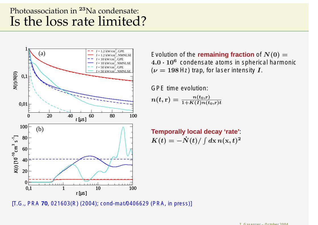
Evolution of the remaining fraction of N(0) =4.0 · 106 condensate atoms in spherical harmonic(ν = 198 Hz) trap, for laser intensity I.

GPE time evolution:

n(t, r) = n(t0,r)1+K(I)n(t0,r)t

Temporally local decay ‘rate’:K(t) = −N(t)/

∫dxn(x, t)2

[T.G., PRA 70, 021603(R) (2004); cond-mat/0406629 (PRA, in press)]

12



0 20 40 60 80 100t [µs]

0,01

0,1

1

N(t

)/N

(0)

I = 1.2 kW/cm2, GPE


I = 10 kW/cm2, GPE


0,1 1 10 100t [µs]

0

20

40

60

80

100

K(t

)[1

0-10 cm

3 s-1

]

(a)

(b)


GPE time evolution:

n(t, r) = n(t0,r)1+K(I)n(t0,r)t


∫dxn(x, t)2


0 20 40 60 80 100t [µs]

0,01

0,1

1

N(t

)/N

(0)

I = 1.2 kW/cm2, GPE


I = 10 kW/cm2, GPE



0,1 1 10 100t [µs]

0

20

40

60

80

100

K(t

)[1

0-10 cm

3 s-1

]

(a)

(b)

12-a



0 20 40 60 80 100t [µs]

0,01

0,1

1

N(t

)/N

(0)

I = 1.2 kW/cm2, GPE


I = 10 kW/cm2, GPE


0,1 1 10 100t [µs]

0

20

40

60

80

100

K(t

)[1

0-10 cm

3 s-1

]

(a)

(b)


GPE time evolution:

n(t, r) = n(t0,r)1+K(I)n(t0,r)t


∫dxn(x, t)2


0 20 40 60 80 100t [µs]

0,01

0,1

1

N(t

)/N

(0)

I = 1.2 kW/cm2, GPE


I = 10 kW/cm2, GPE



0,1 1 10 100t [µs]

0

20

40

60

80

100

K(t

)[1

0-10 cm

3 s-1

]

(a)

(b)

0 20 40 60 80 100t [µs]

0,01

0,1

1

N(t

)/N

(0)

I = 1.2 kW/cm2, GPE


I = 10 kW/cm2, GPE


I = 50 kW/cm2, GPE


0,1 1 10 100t [µs]

0

20

40

60

80

100

K(t

)[1

0-10 cm

3 s-1

]

(a)

(b)

12-b



0 20 40 60 80 100t [µs]

0,01

0,1

1

N(t

)/N

(0)

I = 1.2 kW/cm2, GPE


I = 10 kW/cm2, GPE


0,1 1 10 100t [µs]

0

20

40

60

80

100

K(t

)[1

0-10 cm

3 s-1

]

(a)

(b)


GPE time evolution:

n(t, r) = n(t0,r)1+K(I)n(t0,r)t


∫dxn(x, t)2


0 20 40 60 80 100t [µs]

0,01

0,1

1

N(t

)/N

(0)

I = 1.2 kW/cm2, GPE


I = 10 kW/cm2, GPE



0,1 1 10 100t [µs]

0

20

40

60

80

100

K(t

)[1

0-10 cm

3 s-1

]

(a)

(b)

0 20 40 60 80 100t [µs]

0,01

0,1

1

N(t

)/N

(0)

I = 1.2 kW/cm2, GPE


I = 10 kW/cm2, GPE


I = 50 kW/cm2, GPE


0,1 1 10 100t [µs]

0

20

40

60

80

100

K(t

)[1

0-10 cm

3 s-1

]

(a)

(b)

0 20 40 60 80 100t [µs]

0,01

0,1

1

N(t

)/N

(0)

I = 1.2 kW/cm2, GPE


I = 10 kW/cm2, GPE



I = 50 kW/cm2, GPE

0,1 1 10 100t [µs]

0

20

40

60

80

100

K(t

)[1

0-10 cm

3 s-1

]

(a)

(b)

Max. local decay rate according toKJ(R, t) = (~/m)[nc(R, t)]

−1/3 (hatched)

12-c

Is the molecule formation rate limited?Photoassociation in 23Na condensate:


0 10 20 30 40 50Imax [kW cm

-2]

0,5

0,6

0,7

0,8

0,9

1

1-

Ni(t

fin)/

Nc(0

)

condensate loss, NMNLSE (trap calc.)condensate loss, GPE (local density calc.)

0,001 0,01 0,1 1 100

0,2

0,4

0,6

0,8

1

Fraction of condensate atoms lost aftert = 100µs (red squares).

13



0 10 20 30 40 50Imax [kW cm

-2]

0,5

0,6

0,7

0,8

0,9

1

1-

Ni(t

fin)/

Nc(0

)

condensate loss, NMNLSE (trap calc.)condensate loss, GPE (local density calc.)

0,001 0,01 0,1 1 100

0,2

0,4

0,6

0,8

1

Fraction of condensate atoms lost aftert = 100µs (red squares).

0 10 20 30 40 50Imax [kW cm

-2]

0,5

0,6

0,7

0,8

0,9

1

1-

Ni(t

fin)/

Nc(0

)

condensate loss, NMNLSE (trap calc.)ground state molecules, NMNLSE (trap calc.)condensate loss, GPE (local density calc.)

0,001 0,01 0,1 1 100

0,2

0,4

0,6

0,8

1

Compare this fraction to the fraction ofthe number of atoms lost via spontaneousdecay (green diamonds):

~Ntot = −γ

∫

dR |

∫

dr φ∗

ν(r)Φcl(R, r, t)|2.

( J = 1, ν = 135 )


pote

ntia

l ene

rgy

V(r

)background channel

closed channel

ω = (2π) 80.7 THzγ-1 = 8.6 ns

(32S

1/2 + 3

2S

1/2)

(32S

1/2 + 3

2P

1/2)- ∆

Vbg

(r)

Vcl

(r)

|φν>

13-a

Two-body dressed states

14

Long range nature of dressed statesSaturation of loss rates due to


1 10 100 1000 10000 1e+05r [aBohr]

1e-05

0,0001

0,001

0,01

(4π)

r2 |φdbg

(r)|

2[1

/aB

ohr]

I = 1.0 kW/cm2

I = 10 kW/cm2

-1000 -800 -600 -400 -200 0 200(∆

0-∆)/I [(2π) MHz kW

-1cm

2]

0

20

40

60

80

100

Pop

ulat

ion

[%]

I = 0.1 kW cm-2

I = 1.0 kW cm-2

I = 10 kW cm-2

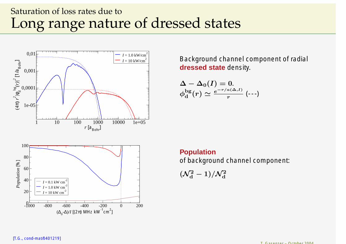
Background channel component of radialdressed state density.

∆ − ∆0(I) = 0.

φbgd (r) ' e−r/a(∆,I)

r(- - -)

Populationof background channel component:

(N 2d − 1)/N 2

d

[T.G., cond-mat/0401219]

15

Background channel dressed state componentPopulation of


0,001 0,01 0,1 1 10 100

Imax [kW cm-2

]

0

20

40

60

80

100

Pop

ulat

ion

[%]

Population (N 2d − 1)/N 2

d of backgroundchannel component vs. intensity I (on reso-nance, ∆ = ∆0(I)).

(

φbgd

φcld

)

= N −1d

(

Gbg(Ed)Wφν

φν

)

0 10 20 30 40 50Imax [kW cm

-2]

0,5

0,6

0,7

0,8

0,9

1

1-

Ni(t

fin)/

Nc(0

)

condensate loss, NMNLSE (trap calc.)ground state molecules, NMNLSE (trap calc.)condensate loss, GPE (local density calc.)

0,001 0,01 0,1 1 100

0,2

0,4

0,6

0,8

1

Compare this to the fraction of the number ofatoms lost via spontaneous decay (green dia-monds):

~Ntot = −γ

∫

dR |

∫

dr φ∗

ν(r)Φcl(R, r, t)|2.

16



0 20 40 60 80 100t [µs]

0,01

0,1

1

Ni(t

)/N

(0)

I = 1.2 kW/cm2

I = 10 kW/cm2

I = 50 kW/cm2

Ntot

Nc

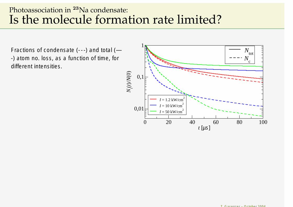
Fractions of condensate (- - -) and total (—-) atom no. loss, as a function of time, fordifferent intensities.

17

OutlookOpen Questions


• Photoassociation:– heteronuclear PA, STIRAP, ...– Alkaline earth elements: small decay width γ, large scattering lengths

(→ metrology)– non-universal observables (many-body frequency shifts)

• Fermionic and mixed systems:– Molecular BEC– BCS pairing

• Improved truncation schemes on the basis of the 2PI effective action

Γ[Ψ, G] = S[Ψ] + i2Tr ln(G−1 +G−1

0 (Ψ)G) + Γ2[Ψ, G]

[G. Aarts, et al., PRD 66, 045008 (2002)]

• Condensates in microtraps: far-from-equilibrium dynamics in (quasi) one-dimensional regime

• Long-time evolution (damping, drifting, thermalization)18

in a Bose-Einstein condensate - pks.mpg.demesuma04/CONTRIBUTIONS/gasenzer-neu.pdfPhotoassociation...

Documents

Transcript of in a Bose-Einstein condensate - pks.mpg.demesuma04/CONTRIBUTIONS/gasenzer-neu.pdfPhotoassociation...