IMU Preintegration on Manifold for EfficientVisual-Inertial Maximum-a-Posteriori Estimation

Christian Forster∗, Luca Carlone†, Frank Dellaert†, and Davide Scaramuzza∗∗Robotics and Perception Group, University of Zurich, Switzerland. Email: {forster,sdavide}@ifi.uzh.ch

†School of Interactive Computing, Georgia Institute of Technology, Atlanta, GA, USA.Email: luca.carlone@gatech.edu, frank@cc.gatech.edu

Abstract—Recent results in monocular visual-inertial navi-gation (VIN) have shown that optimization-based approachesoutperform filtering methods in terms of accuracy due to theircapability to relinearize past states. However, the improvementcomes at the cost of increased computational complexity. In thispaper, we address this issue by preintegrating inertial measure-ments between selected keyframes. The preintegration allows usto accurately summarize hundreds of inertial measurements intoa single relative motion constraint. Our first contribution is apreintegration theory that properly addresses the manifold struc-ture of the rotation group and carefully deals with uncertaintypropagation. The measurements are integrated in a local frame,which eliminates the need to repeat the integration when thelinearization point changes while leaving the opportunity forbelated bias corrections. The second contribution is to show thatthe preintegrated IMU model can be seamlessly integrated in avisual-inertial pipeline under the unifying framework of factorgraphs. This enables the use of a structureless model for visualmeasurements, further accelerating the computation. The thirdcontribution is an extensive evaluation of our monocular VINpipeline: experimental results confirm that our system is very fastand demonstrates superior accuracy with respect to competitivestate-of-the-art filtering and optimization algorithms, includingoff-the-shelf systems such as Google Tango [1].

I. INTRODUCTION

The fusion of cameras and inertial sensors for three-dimensional structure and motion estimation has receivedconsiderable interest in the robotics community. Both sensortypes are cheap, ubiquitous, and complementary. A singlemoving camera is an exteroceptive sensor that allows usto measure appearance and geometry of a three-dimensionalscene, up to an unknown metric scale; an inertial measurementunit (IMU) is a proprioceptive sensor that renders metric scaleof monocular vision and gravity observable [2] and providesrobust and accurate inter-frame motion estimates. Applicationsof VIN range from autonomous navigation in GPS-deniedenvironments, to 3D reconstruction, and augmented reality.

Although impressive results have been achieved in VIN,state-of-the-art algorithms require trading-off computationalefficiency with accuracy. Batch non-linear optimization, whichhas become popular for visual-inertial fusion [3–15], allowscomputing an optimal estimate; however, real-time operation

This research was partially funded by the Swiss National Foundation(project number 200021-143607, “Swarm of Flying Cameras”), the Na-tional Center of Competence in Research Robotics (NCCR), the UZHForschungskredit, the NSF Award 11115678, and the USDA NIFA AwardGEOW-2014-09160.

0 5 10 15 20x [m]

−2

0

2

4

6

8

10

z[m

]

Proposed

Tango

−4 −2 0 2 4 6 8

y [m]

0

5

10

15

20

x[m

]

Fig. 1: Real test comparing the proposed VIN approach against Google Tango.The 160m-long trajectory starts at (0, 0, 0) (ground floor), goes up till the3rd floor of a building, and returns to the initial point. The figure showsa side view (left) and a top view (right) of the trajectory estimates for ourapproach (blue) and Tango (red). Google Tango accumulates 1.4m error, whilethe proposed approach only has 0.5m drift. 3D points triangulated from ourtrajectory estimate are shown in green for visualization purposes.

quickly becomes infeasible as the trajectory and the mapgrow over time. Therefore, it has been proposed to discardframes except selected keyframes [9, 16–18] or to run theoptimization in a parallel thread, using a tracking and mappingdual architecture [5, 19]. Another approach is to maintain alocal map of fixed size and to marginalize old states [6, 7, 9],which is also termed fixed-lag smoothing. To that extreme,if only the latest sensor state is maintained, we speak offiltering, which amounts the vast majority of related workin VIN [20, 21]. Although filtering and fixed-lag smoothingenable fast computation, they commit to a linearization pointwhen marginalizing; the gradual build-up of linearizationerrors leads to drift and possible inconsistencies [22]. Abreakthrough in the direction of reconciling filtering and batchoptimization has been the development of incremental smooth-ing techniques (iSAM [23], iSAM2 [24]), which leverage theexpressiveness of factor graphs to identify and update onlythe typically small subset of variables affected by a newmeasurement. Although this results in constant update timein odometry problems, previous VIN applications still work atlow frame rates [25].

In this work, we present a system that uses incrementalsmoothing for fast computation of the optimal maximum aposteriori (MAP) estimate. The first step towards this goalis the development of a novel preintegration theory. The useof preintegrated IMU measurements was first proposed in[26] and consists of combining many inertial measurementsbetween two keyframes into a single relative motion constraint.

We build upon this work and present a preintegration theorythat properly addresses the manifold structure of the rotationgroup and allows for analytic derivation of all Jacobians.This is in contrast to [26], which adopted Euler angles asglobal parametrization for rotations. Using Euler angles andapplying the usual averaging and smoothing techniques ofEuclidean spaces for state propagation and covariance esti-mation is not properly invariant under the action of rigidtransformations [27]. Moreover, Euler angles are known tohave singularities. Our theoretical derivation in Section Valso advances previous works [10, 12, 13, 25] that usedpreintegrated measurements but did not develop the corre-sponding theory for uncertainty propagation and a-posterioribias correction. Besides these improvements, our model stillbenefits from the pioneering insight of [26]: the integration isperformed in a local frame, which does not require to repeatthe integration when the linearization point changes.

As a second contribution, we frame our preintegrated IMUmodel into a factor graph perspective. This enables the designof a constant-time VIN pipeline based on iSAM2 [24]. Ourincremental-smoothing solution avoids the accumulation oflinearization errors and provides an appealing alternative tousing an adaptive support window for optimization [10].

Inspired by [20, 28], we adopt a structureless model forvisual measurements, which allows eliminating large numbersof variables (i.e., all 3D points) during incremental smoothing,further accelerating the computation.

The third contribution is an efficient implementation andextensive evaluation of our system. Experimental results high-light that our back-end requires an average CPU time of 10msto compute the full MAP estimate and achieves superior ac-curacy with respect to competitive state-of-the-art approaches.The paper is accompanied by supplementary material [29]that reports extra details of our derivation. Furthermore, werelease our implementation of the IMU preintegration and thestructurless vision factors in the GTSAM 4.0 optimizationtoolbox [30]. A video showing an example of the executionof our system is available at https://youtu.be/CsJkci5lfco

II. PRELIMINARIES

A. Notions of Riemannian geometry

This section recalls useful concepts related to the SpecialOrthogonal Group SO(3) and the Special Euclidean GroupSE(3). Our presentation is based on [31, 32].

a) Special Orthogonal Group: SO(3) describes thegroup of 3D rotation matrices and it is formally defined asSO(3)

.= {R ∈ R3×3 : RTR = I,det(R) = 1}. The group

operation is the usual matrix multiplication, and the inverse isthe matrix transpose. The group SO(3) also forms a smoothmanifold. The tangent space to the manifold (at the identity)is denoted so(3), which is also called the Lie algebra andcoincides with the space of 3 × 3 skew symmetric matrices.We can identify every skew symmetric matrix with a vector

SO(3)

so(3)

δφ

Log(R)

φ

R

Exp(φ + δφ)

Exp(Jr(φ)δφ)

Fig. 2: The right Jacobian Jr relates an additive perturbation δφ in the tangentspace to a multiplicative perturbation on the manifold SO(3), as per Eq. (7).

in R3 using the hat operator:

ω∧ =

ω1

ω2

ω3

∧ =

0 −ω3 ω2

ω3 0 −ω1

−ω2 ω1 0

∈ so(3). (1)

Similarly, we can map a skew symmetric matrix to a vector inR3 using the vee operator (·)∨: for a skew symmetric matrixS = ω∧, the vee operator is such that S∨ = ω. A property ofskew symmetric matrices that will be useful later on is:

a∧b = −b∧a, ∀ a,b ∈ R3. (2)

The exponential map (at the identity) exp : so(3)→ SO(3)associates an element of the Lie Algebra to a rotation:

exp(φ∧) = I + sin(‖φ‖)‖φ‖ φ∧ + 1−cos(‖φ‖)

‖φ‖2(φ∧)2. (3)

A first-order approximation of the exponential map is:

exp(φ∧) ≈ I + φ∧ . (4)

The logarithm map (at the identity) associates a matrix R

in SO(3) to a skew symmetric matrix:

log(R) =ϕ · (R− RT)

2 sin(ϕ)with ϕ = cos−1

(tr (R)− 1

2

). (5)

Note that log(R)∨ = aϕ, where a and ϕ are the rotation axisand the rotation angle of R, respectively.

The exponential map is a bijection if restricted to the openball ‖φ‖ < π, and the corresponding inverse is the logarithmmap. However, if we do not restrict the domain, the exponen-tial map becomes surjective as every vector φ = (ϕ+ 2kπ)a,k ∈ Z would be an admissible logarithm of R.

For notational convenience, we adopt “vectorized” versionsof the exponential and logarithm map:

Exp : R3 3 φ → exp(φ∧) ∈ SO(3),Log : SO(3) 3 R → log(R)∨ ∈ R3,

(6)

which operate directly on vectors, rather than on so(3).Later, we will use the following first-order approximation:

Exp(φ+ δφ) ≈ Exp(φ) Exp(Jr(φ)δφ). (7)

The term Jr(φ) is the right Jacobian of SO(3) [31, p.40] andrelates additive increments in the tangent space to multiplica-tive increments applied on the right-hand-side (Fig. 2):

Jr(φ) = I− 1−cos(‖φ‖)‖φ‖2 φ∧ + ‖φ‖−sin(‖φ‖)

‖φ3‖ (φ∧)2. (8)

A similar first-order approximation holds for the logarithm:

Log(

Exp(φ) Exp(δφ))≈ φ+ J−1

r (φ)δφ. (9)

An explicit expression for the inverse of the right Jacobian isgiven in the supplementary material [29]. Jr(φ) reduces to theidentity for ‖φ‖=0.

Another useful property of the exponential map that followsdirectly from the Adjoint representation is:

R Exp(φ) RT = exp(Rφ∧RT) = Exp(Rφ) (10)

⇔ Exp(φ) R = R Exp(RTφ) (11)

b) Special Euclidean Group: SE(3) describes the groupof rigid motion in 3D and it is defined as SE(3)

.=

{(R,p) : R ∈ SO(3),p ∈ R3}. The group operation is T1·T2 =(R1R2 , R1p2 + p1), and the inverse is T−1

1 = (RT1 , −RT1 p1).The exponential map and the logarithm map for SE(3) aredefined in [32]. However, these are not needed in this paperfor reasons that will be clear in Section II-C.

B. Uncertainty Description in SO(3)

A fairly natural definition of uncertainty in SO(3) is todefine a distribution in the tangent space, and then map itto SO(3) via the exponential map (6) [32–34]:

R = R Exp(ε), ε ∼ N (0,Σ), (12)

where R is a given noise-free rotation (the mean) and ε is asmall normally distributed perturbation with zero mean.

The distribution of the random variable R ∈ SO(3) can becomputed explicitly, as shown in [33], leading to:

p(R) = β(R) e−12‖Log(R−1R)‖2

Σ (13)

where β(R) is a normalization factor that can be safely ap-proximated as β(R)'1/

√2π det(Σ) when Σ is small. If we

approximate β as a constant, the negative log-likelihood of arotation R given a measurement R distributed as in (13) is:

L(R) =1

2

∥∥Log(R−1R)∥∥2

Σ+const =

1

2

∥∥Log(R−1R)∥∥2

Σ+const

C. Gauss-Newton Method on Manifold

Let us consider the optimization problem minx∈M f(x),where f(·) is a given cost function, and the variable x belongsto a manifoldM; for simplicity we consider a single variable,while the description can be easily generalized.

A standard approach for optimization on manifold [35, 36],consists of defining a retraction Rx, which is a bijective mapbetween an element δx of the tangent space (at x) and aneighborhood of x ∈ M. Using the retraction, we can re-parametrize our problem as follows:

minx∈M

f(x) ⇒ minδx∈Rn

f(Rx(δx)) (14)

The re-parametrization is usually called lifting [35]. Roughlyspeaking, we work in the tangent space defined at the currentestimate, which locally behaves as an Euclidean space. We cannow apply standard optimization techniques to the problemon the right in (14). In the GN framework, we square thecost around the current estimate. Then we solve the quadraticapproximation to get a vector δx? in the tangent space. Finally,the current guess on the manifold is updated as x← Rx(δx?).

TWB.= (RWB,Wp)

ρl

TBC

Body/IMUCam

World

zl

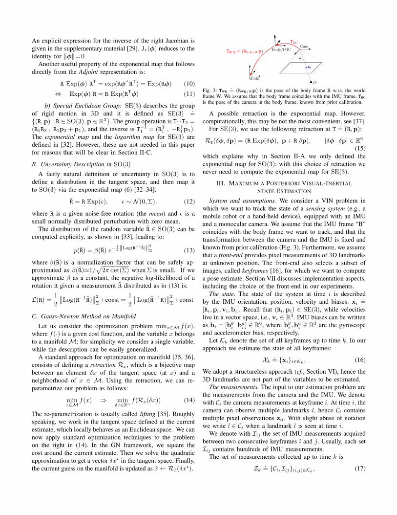
Fig. 3: TWB.= (RWB, Wp) is the pose of the body frame B w.r.t. the world

frame W. We assume that the body frame coincides with the IMU frame. TBC

is the pose of the camera in the body frame, known from prior calibration.

A possible retraction is the exponential map. However,computationally, this may be not the most convenient, see [37].

For SE(3), we use the following retraction at T .= (R,p):

RT(δφ, δp) = (R Exp(δφ), p + R δp), [δφ δp] ∈ R6

(15)which explains why in Section II-A we only defined theexponential map for SO(3): with this choice of retraction wenever need to compute the exponential map for SE(3).

III. MAXIMUM A POSTERIORI VISUAL-INERTIALSTATE ESTIMATION

System and assumptions. We consider a VIN problem inwhich we want to track the state of a sensing system (e.g., amobile robot or a hand-held device), equipped with an IMUand a monocular camera. We assume that the IMU frame “B”coincides with the body frame we want to track, and that thetransformation between the camera and the IMU is fixed andknown from prior calibration (Fig. 3). Furthermore, we assumethat a front-end provides pixel measurements of 3D landmarksat unknown position. The front-end also selects a subset ofimages, called keyframes [16], for which we want to computea pose estimate. Section VII discusses implementation aspects,including the choice of the front-end in our experiments.

The state. The state of the system at time i is describedby the IMU orientation, position, velocity and biases: xi

.=

[Ri,pi,vi,bi]. Recall that (Ri,pi) ∈ SE(3), while velocitieslive in a vector space, i.e., vi ∈ R3. IMU biases can be writtenas bi = [bgi bai ] ∈ R6, where bgi ,b

ai ∈ R3 are the gyroscope

and accelerometer bias, respectively.Let Kk denote the set of all keyframes up to time k. In our

approach we estimate the state of all keyframes:

Xk .= {xi}i∈Kk

. (16)

We adopt a structureless approach (cf., Section VI), hence the3D landmarks are not part of the variables to be estimated.

The measurements. The input to our estimation problem arethe measurements from the camera and the IMU. We denotewith Ci the camera measurements at keyframe i. At time i, thecamera can observe multiple landmarks l, hence Ci containsmultiple pixel observations zil. With slight abuse of notationwe write l ∈ Ci when a landmark l is seen at time i.

We denote with Iij the set of IMU measurements acquiredbetween two consecutive keyframes i and j. Usually, each setIij contains hundreds of IMU measurements.

The set of measurements collected up to time k is

Zk .= {Ci, Iij}(i,j)∈Kk

, (17)

Structureless Projection Factor

Preintegrated IMU FactorIMU Measurements

3D Landmark

Keyframes

Camera Frames

Fig. 4: Left: visual and inertial measurements in VIN. Right: factor graph inwhich several IMU measurements are summarized in a single preintegratedIMU factor and a structureless vision factor constraints keyframes observingthe same landmark.

Factor graphs and MAP estimation. A factor graph encodesthe posterior probability of the variables Xk, given the avail-able measurements Zk and priors p(X0):

p(Xk|Zk) ∝ p(X0)p(Zk|Xk) = p(X0)∏

(i,j)∈Kk

p(Ci, Iij |Xk)

= p(X0)∏

(i,j)∈Kk

p(Iij |xi,xj)∏i∈Kk

∏l∈Ci

p(zil|xi). (18)

The terms in the factorization (18) are called factors. Aschematic representation of the connectivity of the factor graphunderlying the problem is given in Fig. 4 (the connectivity ofthe structureless vision factors will be clarified in Section VI).

The MAP estimate corresponds to the maximum of (18), orequivalently, the minimum of the negative log-posterior. Underthe assumption of zero-mean Gaussian noise, the negative log-posterior can be written a sum of squared residual errors:

X ?k.= arg min

Xk

− loge p(Xk|Zk) (19)

= arg minXk

‖r0‖2Σ0+

∑(i,j)∈Kk

‖rIij‖2Σij+∑i∈Kk

∑l∈Ci

‖rCil‖2ΣC

where r0, rIij , rCil are the residual errors associated to themeasurements, and Σ0, Σij , and ΣC are the correspondingcovariance matrices. The goal of the following sections is toprovide expressions for the residual errors.

IV. IMU MODEL AND MOTION INTEGRATION

An IMU measures the rotation rate and the acceleration ofthe sensor with respect to an inertial frame. The measurements,namely Ba(t), and BωWB(t), are affected by additive white noiseη and a slowly varying sensor bias b:

BωWB(t) = BωWB(t) + bg(t) + ηg(t) (20)

Ba(t) = RTWB(t) (Wa(t)− Wg) + ba(t) + ηa(t), (21)

In our notation, the prefix B denotes that the correspondingquantity is expressed in the frame B (c.f., Fig. 3). The poseof the IMU is described by the transformation {RWB, Wp},which maps a point from sensor frame B to W. The vectorBωWB(t)∈R3 is the instantaneous angular velocity of B relativeto W expressed in coordinate frame B, while Wa(t)∈R3 is theacceleration of the sensor; Wg is the gravity vector in worldcoordinates. We neglect effects due to earth’s rotation, whichamounts to assuming that W is an inertial frame.

The goal now is to infer the motion of the system from IMUmeasurements. For this purpose we introduce the following

Images:

IMU:

Keyframes:

i j

Pre-Int. IMU:

i + 1

k

∆t

Fig. 5: Different rates for IMU and camera.

kinematic model [38, 39]:

RWB = RWB Bω∧WB, Wv = Wa, Wp = Wv, (22)

which describes the evolution of the pose and velocity of B.The state at time t+∆t is obtained by integrating Eq. (22).

Applying Euler integration, which is exact assuming that Waand BωWB remain constant in the interval [t, t+ ∆t], we get:

RWB(t+ ∆t) = RWB(t) Exp (BωWB(t)∆t)

Wv(t+ ∆t) = Wv(t) + Wa(t)∆t

Wp(t+ ∆t) = Wp(t) + Wv(t)∆t+1

2Wa(t)∆t2. (23)

Using Eqs. (20)–(21), we can compute Wa and BωWB as afunction of the IMU measurements, hence (23) becomes

R(t+ ∆t) = R(t) Exp((ω(t)− bg(t)− ηgd(t)

)∆t)

v(t+ ∆t) = v(t) + g∆t+ R(t)(a(t)−ba(t)−ηad(t)

)∆t

p(t+ ∆t) = p(t) + v(t)∆t+1

2g∆t2

+1

2R(t)

(a(t)−ba(t)−ηad(t)

)∆t2, (24)

where we dropped the coordinate frame subscripts for read-ability (the notation should be unambiguous from now on).The covariance of the discrete-time noise ηgd is a function ofthe sampling rate and relates to the continuous-time spectralnoise ηg via Cov(ηgd(t)) = 1

∆tCov(ηg(t)), and the samerelation holds for ηad (cf., [40, Appendix]).

V. IMU PREINTEGRATION ON MANIFOLD

This section contains the first key contribution of the paper.While Eq. (24) could be readily seen as a probabilisticconstraint in a factor graph, it would require to include statesin the factor graph at high rate. Here we show that allmeasurements between two keyframes at times k = i andk = j can be summarized in a single compound measurement,named preintegrated IMU measurement, which constrains themotion between consecutive keyframes. This concept was firstproposed in [26] using Euler angles and we extend it, bydeveloping a suitable theory for preintegration on manifold.

We assume that the IMU is synchronized with the cameraand provides measurements at discrete times k (cf., Fig. 5).1

1We calibrate the IMU-camera delay using the Kalibr toolbox [41]. Analternative is to add the delay as a state in the estimation process [42].

Iterating the IMU integration (24) for all ∆t intervalsbetween k = i and k = j (c.f., Fig. 5), we find:

Rj = Ri

j−1∏k=i

Exp((ωk − bgk − η

gdk

)∆t),

vj = vi+ g∆tij +

j−1∑k=i

Rk

(ak − bak − ηadk

)∆t (25)

pj = pi+

j−1∑k=i

vk∆t+1

2g∆t2ij +

1

2

j−1∑k=i

Rk

(ak−bak−ηadk

)∆t2

where we introduced the shorthands ∆tij.=∑jk=i ∆t and

(·)i .= (·)(ti) for readability.While Eq. (25) already provides an estimate of the motion

between time ti and tj , it has the drawback that the integrationin (25) has to be repeated whenever the linearization point attime ti changes (intuitively, a change in the rotation Ri impliesa change in all future rotations Rk, k = i, . . . , j−1, and makesnecessary to re-evaluate summations and products in (25)).

Our goal is to avoid repeated integrations. For this purpose,we define the following relative motion increments that areindependent of the pose and velocity at ti:

∆Rij.= RTi Rj =

∏j−1k=i Exp

((ωk − bgk − η

gdk

)∆t)

∆vij.= RTi (vj−vi−g∆tij)=

∑j−1k=i ∆Rik

(ak−bak−ηadk

)∆t

∆pij.= RTi

(pj − pi − vi∆tij − 1

2g∆t2ij)

=∑j−1k=i

[∆vik∆t+ 1

2∆Rik(ak−bak−ηadk

)∆t2

]=∑j−1k=i

[32∆Rik

(ak−bak−ηadk

)∆t2

](26)

where we defined ∆Rik.= RTi Rk and ∆vik

.= vk − vi.

Unfortunately, summations and products in (26) are stillfunction of the bias. We tackle this problem in two steps.In Section V-A, we assume bi is known; then, in Section V-Cwe show how to avoid repeating the integration when the biasestimate changes. In the rest of the paper, we assume that thebias remains constant between two keyframes:

bgi = bgi+1 = . . . = bgj−1, bai = bai+1 = . . . = baj−1. (27)

A. Preintegrated IMU Measurements

In this section, we assume that the bias at time ti is known.We want to isolate the noise in (26). Therefore, starting withthe rotation increment ∆Rij , we use the first-order approxi-mation (7) (rotation noise is “small”) and rearrange the terms,by “moving” the noise to the end, using the relation (11):

∆Rijeq.(7)'

j−1∏k=i

[Exp ((ωk − bgi ) ∆t) Exp

(−Jkr ηgdk ∆t

)]eq.(11)

= ∆Rij

j−1∏k=i

Exp(−∆RTk+1j J

kr η

gdk ∆t

).= ∆RijExp

(−δφij

)(28)

with Jkr.= Jkr (ωk−bgi ). We defined the preintegrated rotation

measurement ∆Rij.=∏j−1k=i Exp ((ωk − bgi ) ∆t), and its

noise δφij , which will be further analysed in the next section.

Substituting (28) back into the expression of ∆vij in (26),using the approximation (4) for Exp

(−δφij

), and dropping

higher-order noise terms, we obtain:

∆vijeq.(4)'

j−1∑k=i

∆Rik(I− δφ∧ik) (ak−bai ) ∆t−∆Rikηadk ∆t

eq.(2)= ∆vij+

j−1∑k=i

[∆Rik (ak−bai )

∧δφik∆t−∆Rikη

adk ∆t

].= ∆vij − δvij (29)

where we defined the preintegrated velocity measurement∆vij

.=∑j−1k=i∆Rik(ak−bai ) ∆t and its noise δvij .

Similarly, substituting (28) in the expression of ∆pijin (26), and using the first-order approximation (4), we obtain:

∆pijeq.(4)'

j−1∑k=i

3

2∆Rik(I−δφ∧ik) (ak−bai ) ∆t2−

j−1∑k=i

3

2∆Rikη

adk ∆t2

eq.(2)= ∆pij+

j−1∑k=i

[3

2∆Rik (ak−bai )

∧δφik∆t2− 3

2∆Rikη

adk ∆t2

].= ∆pij − δpij (30)

where we defined the preintegrated position measurement∆pij and its noise δpij .

Substituting the expressions (28), (29), (30) back in theoriginal definition of ∆Rij ,∆vij ,∆pij in (26), we finally getour preintegrated measurement model:

∆Rij = RTi RjExp(δφij

)∆vij = RTi (vj−vi−g∆tij) + δvij

∆pij = RTi

(pj − pi − vi∆tij −

1

2g∆t2ij

)+ δpij (31)

where our compound measurements are written as a functionof the (to-be-estimated) state “plus” a random noise, describedby the random vector [δφT

ij , δvTij , δp

Tij ]

T. The nature of thenoise terms is discussed in the following section.

B. Noise Propagation

Let us start with the rotation noise:

Exp(−δφij

) .=∏j−1k=i Exp

(−∆RTk+1jJ

kr η

gdk ∆t

). (32)

Taking the Log at both members and changing signs, we get:

δφij = −Log(∏j−1

k=i Exp(−∆RTk+1jJ

kr η

gdk ∆t

)). (33)

Repeated application of the first-order approximation (9) (re-call that ηgdk as well as δφij are small rotation noises, hencethe right Jacobians are close to the identity) produces:

δφij '∑j−1k=i ∆RTk+1j J

kr η

gdk ∆t (34)

Up to first order, the noise δφij is zero-mean and Gaussian, asit is a linear combination of zero-mean noise terms ηgdk . This isdesirable, since it brings the rotation measurement model (31)exactly in the form (12).

Dealing with the noise terms δvij and δpij is now easy:these are linear combinations of the acceleration noise ηadkand the preintegrated rotation noise δφij , hence they are alsozero-mean and Gaussian.

Therefore, we can fully characterize the noise as:

[δφTij , δv

Tij , δp

Tij ]

T ∼ N (09×1,Σij). (35)

The expression for the covariance Σij is provided in thesupplementary material [29], where we also show that boththe preintegrated measurements ∆Rij ,∆vij ,∆pij , and thecovariance Σij can be computed incrementally.

C. Incorporating Bias Updates

In the previous section, we assumed that the bias bi used tocompute the preintegrated measurements is given. However,more likely, the bias estimate changes during optimization.One solution would be to recompute the delta measurementswhen the bias changes; however, that is computationallyexpensive. Instead, given a bias update b ← b + δb, we canupdate the delta measurements using a first-order expansion:

∆Rij(bgi ) ' ∆Rij(b

gi ) Exp

(∂∆Rij∂bg δbg

)∆vij(b

gi ,b

ai ) ' ∆vij(b

gi , b

ai ) +

∂∆vij

∂bg δbgi +∂∆vij

∂ba δbai

∆pij(bgi ,b

ai ) ' ∆pij(b

gi , b

ai ) +

∂∆pij

∂bg δbgi +∂∆pij

∂ba δbai(36)

This is similar to the bias correction in [26] but operates di-rectly on SO(3). The Jacobians {∂∆Rij

∂bg ,∂∆vij

∂bg , . . .} (computedat bi) describe how the measurements change due to a changein the bias estimate. The derivation of the Jacobians is verysimilar to the one we used in Section V-A to express the mea-surements as a large value plus a small perturbation; hence,we omit the complete derivation, which can be found in thesupplementary material [29]. Note that the Jacobians remainconstant and can be precomputed during the preintegration.

D. Preintegrated IMU Factors

Given the preintegrated measurement model in (31) andsince measurement noise is zero-mean and Gaussian up tofirst order (35), it is now easy to write the residual errorsrIij

.= [rT∆Rij

, rT∆vij, rT∆pij

]T ∈ R9, where

r∆Rij

.= Log

((∆Rij(b

gi )Exp

(∂∆Rij∂bg δbg

))TRTi Rj

)r∆vij

.= RTi (vj − vi − g∆tij)

−[∆vij(b

gi , b

ai ) +

∂∆vij

∂bg δbg +∂∆vij

∂ba δba]

r∆pij

.= RTi

(pj − pi − vi∆tij − 1

2g∆t2ij)

−[∆pij(b

gi , b

ai ) +

∂∆pij

∂bg δbg +∂∆pij

∂baδba

], (37)

in which we also included the bias updates of Eq. (36).According to the “lift-solve-retract” method (Section II-C),

at each GN iteration we need to re-parametrize (37) using theretraction (15). Then, the “solve” step requires to linearizethe resulting cost. For the purpose of linearization, it isconvenient to compute analytic expressions of the Jacobiansof the residual errors, which we derive in [29].

E. Bias Model

When presenting the IMU model (20), we said that biasesare slowly time-varying quantities. Hence, we model themwith a “Brownian motion”, i.e., integrated white noise:

bg(t) = ηbg, ba(t) = ηba. (38)

Integrating (38) over the time interval [ti, tj ] between twoconsecutive keyframes i and j we get:

bgj = bgi + ηbgd, baj = bai + ηbad, (39)

where, as done before, we use the shorthand bgi.= bg(ti),

and we define the discrete noises ηbgd and ηbad, which havezero mean and covariance Σbgd .

= ∆tijCov(ηbg) and Σbad .=

∆tijCov(ηba), respectively (cf. [40, Appendix]).The model (39) can be readily included in our factor graph,

as a further additive term in (19) for all consecutive keyframes:

‖rbij‖2.= ‖bgj − bgi ‖2Σbgd + ‖baj − bai ‖2Σbad (40)

VI. STRUCTURELESS VISION FACTORS

In this section we introduce our structureless model forvision measurements. The key feature of our approach is thelinear elimination of landmarks. Note that the elimination isrepeated at each Gauss-Newton iteration, hence we are stillguaranteed to obtain the optimal MAP estimate.

Visual measurements contribute to the cost (19) via the sum:∑i∈Kk

∑l∈Ci ‖rCil‖2ΣC =

∑Ll=1

∑i∈X (l) ‖rCil‖2ΣC (41)

which, on the right-hand-side, we rewrote as a sum of contri-butions of each landmark l = 1, . . . , L. In (41), X (l) denotesthe subset of keyframes in which l is seen.

A fairly standard model for the residual error of a singlepixel measurement zil is [13]:

rCil = zil − π(Ri,pi, ρl), (42)

where ρl ∈ R3 denotes the position of the l-th landmark, andπ(·) is a standard perspective projection, which also encodesthe (known) IMU-camera transformation TBC.

Direct use of (42) would require to include the landmarkpositions ρl, l = 1, . . . , L in the optimization, and this impactsnegatively on computation. Therefore, in the following weadopt a structureless approach that avoids optimization overthe landmarks, thus ensuring to retrieve the MAP estimate.

As recalled in Section II-C, at each GN iteration, we lift thecost function, using the retraction (15). For the vision factorsthis means that the original residuals (41) become:∑L

l=1

∑i∈X (l) ‖zil − π(δφi, δpi, δρl)‖2ΣC (43)

where δφi, δpi, δρl are now Euclidean corrections, and π(·)is the lifted cost function. The “solve” step in the GN methodis based on linearization of the residuals:∑L

l=1

∑i∈X (l) ‖FilδTi + Eilδρl − bil‖2, (44)

where δTi.= [δφi δpi]

T; the Jacobians Fil,Eil, and the vec-tor bil (both normalized by Σ

1/2C ) result from the linearization.

The vector bil is the residual error at the linearization point.

Writing the second sum in (44) in matrix form we get:∑Ll=1 ‖Fl δTX (l) + El δρl − bl‖2 (45)

where Fl,El,bl are obtained by stacking Fil,Eil,bil, respec-tively, for all i ∈ X (l). We can eliminate the variable δρl byprojecting the residual into the null space of El:∑L

l=1

∥∥Q(Fl δTX (l) − bl)∥∥2

(46)

where Q.= I−El(E

Tl El)

−1ETl is an orthogonal projector of

El as shown in the supplementary material [29]. Using thisapproach, we reduced a large set of factors (43) which involveposes and landmarks into a smaller set of L factors (46), whichonly involve poses. In particular, the factor corresponding tolandmark l only involves the states X (l) observing l, creatingthe connectivity pattern of Fig. 4.

VII. IMPLEMENTATION

Our implementation consists of a high frame rate trackingfront-end based on SVO2 [43] and an optimization back-endbased on iSAM23 [24]. The front-end tracks the pose at camerarate while the back-end optimizes in parallel the state ofselected keyframes as described in this paper.

SVO [43] is a precise and robust monocular visual odometrysystem that employs sparse image alignment, which estimatesincremental motion and tracks features by minimizing thephotometric error between subsequent images. Thereby, SVOavoids every-frame feature extraction, resulting in high-frame-rate motion estimation. Combined with an outlier resistantprobabilistic triangulation method, SVO provides increasedrobustness in scenes with repetitive and high frequency texture.

The computation of the MAP estimate in Eq. (19) isbased on iSAM2 [24], which is a state-of-the-art incrementalsmoothing approach. iSAM2 exploits the fact that new mea-surements often have only local effect on the MAP estimate,hence applies incremental updates directly to the square-rootinformation matrix, only re-solving for the variables affectedby the new measurements. In odometry problems, the use ofiSAM2 results in constant-time updates.

VIII. EXPERIMENTS

The first experiment shows that the proposed approachis more accurate than two competitive state-of-the-art ap-proaches, namely ASLAM [9], and MSCKF [20]. The ex-periment is performed on the indoor trajectory of Fig. 6.The dataset was recorded with a forward-looking VI-Sensor[44] that consists of an ADIS16448 MEMS IMU and twoembedded WVGA monochrome cameras (we only use theleft camera). Intrinsic and extrinsic calibration was obtainedusing [41]. The camera runs at 20Hz and the IMU at 800Hz.Ground truth poses are provided by a Vicon system mounted inthe room; the hand-eye calibration between the Vicon markersand the camera is computed using a least-squares method [45].

2http://github.com/uzh-rpg/rpg svo3http://borg.cc.gatech.edu

Fig. 6: Left: two images from the indoor trajectory dataset with trackedfeatures in green. Right: top view of the trajectory estimate produced by ourapproach (blue) and 3D landmarks triangulated from the trajectory (green).

10 40 90 160 250 360

Distance traveled [m]

0.0

0.2

0.4

0.6

0.8

1.0

1.2

1.4

Tra

nsl

atio

ner

ror

[m]

Proposed ASLAM MSCKF

10 40 90 160 250 360

Distance traveled [m]

02468

1012141618

Yaw

erro

r[d

eg]

10 40 90 160 250 360

Distance traveled [m]

0.0

0.5

1.0

1.5

2.0

2.5

Avg.

Pit

chan

dR

oll

err.

[deg

]

Fig. 7: Comparison of the proposed approach versus the ASLAM al-gorithm [9] and an implementation of the MSCKF filter [20]. Relativeerrors are measured over different segments of the trajectory, of length{10, 40, 90, 160, 250, 360}m, according to the odometric error metric in [46].

0 200 400 600 800 1000Keyframe ID

05

10152025303540

Pro

cess

ing

Tim

e[m

s]

Fig. 8: Processing-time per keyframe for the proposed VIN approach.

Fig. 7 compares the proposed system against the ASLAMalgorithm [9], and an implementation of the MSCKF fil-ter [20]. Both these algorithms currently represent the state-of-the-art in VIN, ASLAM for optimization-based approaches,and MSCKF for filtering methods. We obtained the datasets aswell as the trajectories computed with ASLAM and MSCKFfrom the authors of [9]. We use the relative error metricsproposed in [46] to obtain error statistics. The metric eval-uates the relative error by averaging the drift over trajectorysegments of different length ({10, 40, 90, 160, 250, 360}m inFig. 7). Our approach exhibits less drift than the state-of-the-art, achieving 0.3m drift on average over 360m travelled

−60 −40 −20 0 20 40 60

x [m]

0

10

20

30

40

50y

[m]

Proposed

Tango

Fig. 9: Outdoor trajectory (length: 300m) around a building with identical startand end point at coordinates (0, 0, 0). The end-to-end error of the proposedapproach is 1.0m. Google Tango accumulated 2.2m drift. The green dots arethe 3D points triangulated from our trajectory estimate.

distance; ASLAM and MSCKF accumulate an average errorof 0.7m. We observe significantly less drift in yaw directionin the proposed approach while the error in pitch and and rolldirection is constant for all methods due to the observabilityof the gravity direction.

Figure 8 illustrates the time required by the back-end tocompute the full MAP estimate, by running iSAM2 with 10optimization iterations. The experiment was performed on astandard laptop (Intel i7, 2.4 GHz). The average update timefor iSAM2 is 10ms. The peak corresponds to the start of theexperiment in which the camera was not moving. In this casethe number of tracked features becomes very large makingthe back-end slightly slower. The SVO front-end requiresapproximately 3ms to process a frame on the laptop whilethe back-end runs in a parallel thread and optimizes onlykeyframes. Although the processing times of ASLAM werenot reported, the approach is described as computationallydemanding [9]. ASLAM needs to repeat IMU integration atevery change of the linearization point, which we avoid byusing the preintegrated IMU measurements.

The second experiment is performed on an outdoor trajec-tory, and compares the proposed approach against the GoogleTango Peanut sensor (mapper version 3.15), which is anengineered VIN system. We rigidly attached the VI-Sensor toa Tango device and walked around an office building. Fig. 9depicts the trajectory estimates for our approach and GoogleTango. The trajectory starts and ends at the same location,hence we can report the end-to-end error which is 1.5m forthe proposed approach and 2.2m for the Google Tango sensor.

The third experiment is the one in Fig. 1. The trajectorygoes across three floors of an office building and eventuallyreturns to the initial location on the ground floor. Also in thiscase the proposed approach guarantees a very small end-to-enderror (0.5m), while Tango accumulates 1.4m error.

We remark that Tango and our system use different sensors,hence the reported end-to-end errors only allow for a qualita-tive comparison. However, the IMUs of both sensors exhibitsimilar noise characteristics [47, 48] and the Tango camerahas a significantly larger field-of-view and better shutter speedcontrol than our sensor. Therefore, the comparison is stillvaluable to assess the accuracy of the proposed approach.

The fourth experiment evaluates a specific aspect of our

0.04 0.08 0.12 0.16 0.2Bias Change

0.0000000.0000020.0000040.0000060.0000080.0000100.0000120.0000140.0000160.000018

Tra

nsl

atio

nE

rror

[m]

0.04 0.08 0.12 0.16 0.2Bias Change

0.0000

0.0001

0.0002

0.0003

0.0004

0.0005

Vel

oci

tyE

rror

[m/s

]

0.04 0.08 0.12 0.16 0.2Bias Change

0.0000

0.0001

0.0002

0.0003

0.0004

0.0005

0.0006

0.0007

0.0008

Rot

atio

nE

rror

[deg

]

Fig. 10: Error committed when using the first-order approximation (36) insteadof repeating the integration, for different bias perturbations. Left: ∆Rij(bi +δbi) error; Center: ∆vij(bi + δbi) error; Right: ∆pij(bi + δbi) error.Statistics are computed over 1000 Monte Carlo runs.

approach: the a-posteriori bias correction of Section V-C. Toevaluate the quality of the first-order approximation (36), weperformed the following Monte Carlo analysis. First, we com-puted the preintegrated measurements ∆Rij(bi),∆vij(bi) and∆pij(bi) over 100 IMU measurements at a given bias esti-mate bi. Then, we applied a perturbation δbi (in a randomdirection with magnitude between 0.04 and 0.2) to both thegyroscope and accelerometer bias. We repeated the integrationat bi+ δbi, and we obtained ∆Rij(bi+ δbi),∆vij(bi+ δbi)and ∆pij(bi + δbi). Finally, we compared the result of theintegration against the first-order correction in (36). Fig. 10reports statistics of the errors in the preintegrated variablesbetween the re-integrated variables and the first-order correc-tion, over 1000 Monte Carlo runs. The order of magnitude ofthe errors suggests that the first-order approximation capturesvery well the bias change, and can be safely used for relativelylarge bias fluctuations.

A video demonstrating the execution of our approach forthe real experiments discussed in this section can be viewedat https://youtu.be/CsJkci5lfco

IX. CONCLUSION

We propose a novel preintegration theory that provides agrounded way to model a large number of IMU measurementsas a single motion constraint. Our proposal improves overrelated works that perform integration in a global frame,e.g., [8, 20], as we do not commit to a linearization pointduring integration. Moreover, it leverages the seminal workon preintegration [26], bringing to maturity the preintegrationand uncertainty propagation in SO(3). We also discuss howto use the preintegrated IMU model in a VIN pipeline; weadopt a structureless model for visual measurements whichavoids optimizing over 3D landmarks. Our VIN approach usesiSAM2 to perform constant-time incremental smoothing.

An efficient implementation of our approach requires 10msto perform inference (back-end), and 3ms for feature tracking(front-end). We provide comparisons against state-of-the-artalternatives, including filtering and optimization-based tech-niques. We release the source-code of the IMU preintegrationand the structurless vision factors in the GTSAM 4.0 optimiza-tion toolbox [30] and provide additional theoretical derivationsand implementation details in the supplementary material [29].

Acknowledgments The authors gratefully acknowledge StephenWilliams and Richard Roberts for helping with an early implemen-tation in GTSAM, and Simon Lynen and Stefan Leutenegger forproviding datasets and results of their algorithms.

REFERENCES

[1] Google. Project tango. URL https://www.google.com/atap/projecttango/.

[2] A. Martinelli. Vision and IMU data fusion: Closed-form solu-tions for attitude, speed, absolute scale, and bias determination.IEEE Trans. Robotics, 28(1):44–60, 2012.

[3] S-H. Jung and C.J. Taylor. Camera trajectory estimation usinginertial sensor measurements and structure fom motion results.In IEEE Conf. on Computer Vision and Pattern Recognition(CVPR), 2001.

[4] D. Sterlow and S. Singh. Motion estimation from image andinertial measurements. 2004.

[5] A.I. Mourikis and S.I. Roumeliotis. A dual-layer estimatorarchitecture for long-term localization. In Proc. of the Workshopon Visual Localization for Mobile Platforms at CVPR, Anchor-age, Alaska, June 2008.

[6] G. Sibley, L. Matthies, and G. Sukhatme. Sliding window filterwith application to planetary landing. J. of Field Robotics, 27(5):587–608, 2010.

[7] T-C. Dong-Si and A.I. Mourikis. Motion tracking with fixed-lagsmoothing: Algorithm consistency and analysis. In IEEE Intl.Conf. on Robotics and Automation (ICRA), 2011.

[8] S. Leutenegger, P. Furgale, V. Rabaud, M. Chli, K. Konolige,and R. Siegwart. Keyframe-based visual-inertial slam usingnonlinear optimization. In Robotics: Science and Systems (RSS),2013.

[9] S. Leutenegger, S. Lynen, M. Bosse, R. Siegwart, and P. Furgale.Keyframe-based visual-inertial slam using nonlinear optimiza-tion. Intl. J. of Robotics Research, 2014.

[10] N. Keivan, A. Patron-Perez, and G. Sibley. Asynchronousadaptive conditioning for visual-inertial SLAM. In Intl. Sym.on Experimental Robotics (ISER), 2014.

[11] D.-N. Ta, K. Ok, and F. Dellaert. Vistas and parallel tracking andmapping with wall-floor features: Enabling autonomous flightin man-made environments. Robotics and Autonomous Systems,62(11):1657–1667, 2014. doi: http://dx.doi.org/10.1016/j.robot.2014.03.010. Special Issue on Visual Control of Mobile Robots.

[12] S. Shen. Autonomous Navigation in Complex Indoor andOutdoor Environments with Micro Aerial Vehicles. PhD Thesis,University of Pennsylvania, 2014.

[13] V. Indelman, S. Wiliams, M. Kaess, and F. Dellaert. Informationfusion in navigation systems via factor graph based incrementalsmoothing. Robotics and Autonomous Systems, 61(8):721–738,August 2013.

[14] M. Bryson, M. Johnson-Roberson, and S. Sukkarieh. Airbornesmoothing and mapping using vision and inertial sensors. InIEEE Intl. Conf. on Robotics and Automation (ICRA), pages3143–3148, 2009.

[15] A. Patron-Perez, S. Lovegrove, and G. Sibley. A spline-basedtrajectory representation for sensor fusion and rolling shuttercameras. Intl. J. of Computer Vision, February 2015.

[16] H. Strasdat, J.M.M. Montiel, and A.J. Davison. Real-timemonocular SLAM: Why filter? In IEEE Intl. Conf. on Roboticsand Automation (ICRA), pages 2657–2664, 2010.

[17] G. Klein and D. Murray. Parallel tracking and mapping on acamera phone. In IEEE and ACM Intl. Sym. on Mixed andAugmented Reality (ISMAR), 2009.

[18] E.D. Nerurkar, K.J. Wu, and S.I. Roumeliotis. C-KLAM: Con-strained keyframe-based localization and mapping. In Robotics:Science and Systems (RSS), 2013.

[19] G. Klein and D. Murray. Parallel tracking and mapping forsmall AR workspaces. In IEEE and ACM Intl. Sym. on Mixedand Augmented Reality (ISMAR), pages 225–234, Nara, Japan,Nov 2007.

[20] A.I. Mourikis and S.I. Roumeliotis. A multi-state constraintKalman filter for vision-aided inertial navigation. In IEEE Intl.

Conf. on Robotics and Automation (ICRA), pages 3565–3572,April 2007.

[21] E.S. Jones and S. Soatto. Visual-inertial navigation, mappingand localization: A scalable real-time causal approach. Intl. J.of Robotics Research, 30(4), Apr 2011.

[22] G.P. Huang, A.I. Mourikis, and S.I. Roumeliotis. Anobservability-constrained sliding window filter for SLAM. InIEEE/RSJ Intl. Conf. on Intelligent Robots and Systems (IROS),pages 65–72, 2011.

[23] M. Kaess, A. Ranganathan, and F. Dellaert. iSAM: Incrementalsmoothing and mapping. IEEE Trans. Robotics, 24(6):1365–1378, Dec 2008.

[24] M. Kaess, H. Johannsson, R. Roberts, V. Ila, J. Leonard, andF. Dellaert. iSAM2: Incremental smoothing and mapping usingthe Bayes tree. Intl. J. of Robotics Research, 31:217–236, Feb2012.

[25] V. Indelman, A. Melim, and F. Dellaert. Incremental lightbundle adjustment for robotics navigation. In IEEE/RSJ Intl.Conf. on Intelligent Robots and Systems (IROS), November2013.

[26] T. Lupton and S. Sukkarieh. Visual-inertial-aided navigationfor high-dynamic motion in built environments without initialconditions. IEEE Trans. Robotics, 28(1):61–76, Feb 2012.

[27] M. Moakher. Means and averaging in the group of rotations.SIAM Journal on Matrix Analysis and Applications, 24(1):1–16,2002.

[28] L. Carlone, Z. Kira, C. Beall, V. Indelman, and F. Dellaert.Eliminating conditionally independent sets in factor graphs: Aunifying perspective based on smart factors. In IEEE Intl. Conf.on Robotics and Automation (ICRA), 2014.

[29] C. Forster, L. Carlone, F. Dellaert, and D. Scaramuzza. Sup-plementary material to: IMU preintegration on manifold forefficient visual-inertial maximum-a-posteriori estimation. Tech-nical Report GT-IRIM-CP&R-2015-001, Georgia Institute ofTechnology, 2015.

[30] Frank Dellaert. Factor graphs and GTSAM: A hands-on intro-duction. Technical Report GT-RIM-CP&R-2012-002, GeorgiaInstitute of Technology, 2012.

[31] G. S. Chirikjian. Stochastic Models, Information Theory, andLie Groups, Volume 2: Analytic Methods and Modern Applica-tions (Applied and Numerical Harmonic Analysis). Birkhauser,2012.

[32] Y. Wang and G.S. Chirikjian. Nonparametric second-ordertheory of error propagation on motion groups. Intl. J. ofRobotics Research, 27(11–12):1258–1273, 2008.

[33] T. D. Barfoot and P. T. Furgale. Associating uncertainty withthree-dimensional poses for use in estimation problems. IEEETrans. Robotics, 30(3):679–693, 2014.

[34] Y. Wang and G.S. Chirikjian. Error propagation on the euclideangroup with applications to manipulator kinematics. IEEE Trans.Robotics, 22(4):591–602, 2006.

[35] K.A. Gallivan P.A. Absil, C.G. Baker. Trust-region methods onRiemannian manifolds. Foundations of Computational Mathe-matics, 7(3):303–330, 2007.

[36] S. T. Smith. Optimization techniques on Riemannian manifolds.Hamiltonian and Gradient Flows, Algorithms and Control,Fields Inst. Commun., Amer. Math. Soc., 3:113–136, 1994.

[37] J. H. Manton. Optimization algorithms exploiting unitaryconstraints. IEEE Trans. Signal Processing, 50:63–650, 2002.

[38] R.M. Murray, Z. Li, and S. Sastry. A Mathematical Introductionto Robotic Manipulation. CRC Press, 1994.

[39] J.A. Farrell. Aided Navigation: GPS with High Rate Sensors.McGraw-Hill, 2008.

[40] J.L. Crassidis. Sigma-point Kalman filtering for integrated GPSand inertial navigation. IEEE Trans. Aerosp. Electron. Syst., 42(2):750–756, 2006.

[41] P. Furgale, J. Rehder, and R. Siegwart. Unified temporal and

spatial calibration for multi-sensor systems. In IEEE/RSJ Intl.Conf. on Intelligent Robots and Systems (IROS), 2013.

[42] M. Li and A.I. Mourikis. Online temporal calibration forcamera-imu systems: Theory and algorithms. Intl. J. of RoboticsResearch, 33(6), 2014.

[43] C. Forster, M. Pizzoli, and D. Scaramuzza. SVO: Fast Semi-Direct Monocular Visual Odometry. In IEEE Intl. Conf. onRobotics and Automation (ICRA), 2014. doi: 10.1109/ICRA.2014.6906584.

[44] J. Nikolic, J., Rehderand M. Burri, P. Gohl, S. Leutenegger,P. Furgale, and R. Siegwart. A Synchronized Visual-InertialSensor System with FPGA Pre-Processing for Accurate Real-Time SLAM. In IEEE Intl. Conf. on Robotics and Automation(ICRA), 2014.

[45] F.C. Park and B.J. Martin. Robot sensor calibration: SolvingAX=XB on the euclidean group. 10(5), 1994.

[46] A. Geiger, P. Lenz, and R. Urtasun. Are we ready for au-tonomous driving? the KITTI vision benchmark suite. In IEEEConf. on Computer Vision and Pattern Recognition (CVPR),pages 3354–3361, Providence, USA, June 2012.

[47] Tango IMU specifications. URL http://ae-bst.resource.bosch.com/media/products/dokumente/bmx055/BST-BMX055-FL000-00 2013-05-07 onl.pdf.

[48] Adis IMU specifications. URL http://www.analog.com/media/en/technical-documentation/data-sheets/ADIS16448.pdf.