errors, but in most cases, data are missing or erroneous for extendedperiods of time (hours, days). Recently, Chen et al. have used lin-ear regression–based imputation procedures to successfully predictmissing data in freeway main-line loop detector stations (8). Thismethod cannot be applied to impute missing data in on-ramp or off-ramp vehicle detector stations because a high correlation of databetween neighboring ramp loop detector stations cannot be guar-anteed. Hence, model-based imputation procedures are requiredto determine missing ramp flow data. Once the dynamic model offreeway traffic is specified, the unknown quantities can be esti-mated by use of adaptive identification techniques that have beenused in iterative learning control (9, 10). Repetitive identificationalgorithms can be used off-line to determine the flow profiles thatminimize the error between the model-calculated densities and themain-line loop detector measurements.

This paper illustrates an imputation procedure for determiningramp flows using the link–node CTM. The LN-CTM used for trafficflow simulations is reviewed in the following section. A simple four-state switching approximation of the model for freeway-corridorsimulations is also presented. Next, the imputation procedure used fordetermining on-ramp and off-ramp flows is explained. The section onapplication illustrates an example in which the imputation proce-dure is used to specify the on-ramp flows and off-ramp split ratios fora 26-mi-long section of the I-210E freeway in the Los Angeles area.

LINK–NODE CELL TRANSMISSION MODEL

The link–node cell transmission model (LN-CTM) is used to simulatetraffic flows in traffic networks. Aurora, a simulation tool in TOPL,is based on this CTM implementation (11). Other implementations ofthe CTM include the asymmetric cell transmission model (ACTM)used particularly for freeway traffic simulation (12). The link–nodecell transmission model is preferred for simulation because it has thecapability to simulate traffic networks that include freeways and arte-rial networks, as compared with the ACTM, which has been used pri-marily for freeway simulations. As a result, in this paper the link–nodeCTM has been used for imputation of on-ramp and off-ramp flows.

In the LN-CTM the freeway (or any traffic network) is specifiedby a graph of links. Links represent road segments, which carry traf-fic. Nodes are formed at the junction of links, where traffic flowexchange takes place. The flow exchange is indicated by a time-varying split-ratio matrix, which specifies the portion of traffic mov-ing from a particular input link to an output link. Although a normallink connects two nodes, a “source” link is used to introduce trafficinto the network and a “sink” is used to accept traffic moving out ofthe network. A source link implements a queue model.

Figure 1 shows the freeway specified in the link–node framework.Each node contains a maximum of one on- and one off-ramp. The

Imputation of Ramp Flow Data for Freeway Traffic Simulation

Ajith Muralidharan and Roberto Horowitz

The Tools for Operational Planning is a suite of tools that uses thelink–node cell transmission model for macroscopic freeway traffic sim-ulations for specifying operational strategies such as ramp metering anddemand and incident management. Traffic flow and occupancy datafrom loop detectors are used for calibrating these models and specify-ing the inputs to the simulation. Flow data from ramps, however, areoften found to be missing or incorrect. This paper elaborates an imputa-tion procedure used to determine these ramp flows. This automatedimputation procedure is based on an adaptive identification techniquethat attempts to minimize the error between the simulated and the mea-sured densities. Simulation results using the imputed flow data indicategood conformation with loop detector measurements.

The Tools for Operational Planning (TOPL) is a suite of tools usedfor (a) specifying operational improvements, such as ramp meter-ing, incident management, traveler information, and demand man-agement, and (b) quickly estimating the benefits such improvementsare likely to provide. This is an essential component of the Califor-nia Department of Transportation “corridor management program,”which was introduced to reduce congestion by 2025 by 40% (1).

Traditionally, transportation planning investigations favor the useof microscopic models. The microscopic simulations involve exten-sive data collection and model calibration efforts, which are sig-nificantly time-consuming (2). In comparison, macroscopic modelssuch as the cell transmission model (CTM) are based on aggregatevariables such as volume (flow) and density. These data are availablefor California freeways from vehicle detector stations (VDS), whichcontain loop detectors. The freeway performance measurement sys-tem (PeMS) (3) routinely archives the flow, occupancy, and speeddata from these VDS. Therefore, TOPL is based on the macroscopiclink–node cell transmission model (LN-CTM) (4). In general, theCTM requires the flow and density measurements from the main-line VDS (positioned along the freeway) for calibration of the fun-damental diagrams (5). The on-ramp flows and off-ramp split ratiosalso need to be specified as an input for the simulations. However,the data from the ramps are often found to be missing or incorrect.Hence, it becomes essential to impute the on-ramp and off-rampflows to completely specify the simulation model.

Imputation of missing data in loop detectors has been investigatedusing various techniques such as time series analysis (6) and Kalmanfilters (7 ). These methods are useful for prediction of random

Department of Mechanical Engineering, University of California, Berkeley, Etchev-erry Hall, Berkeley, CA 94720. Corresponding author: A. Muralidharan, ajith@berkeley.edu.

Transportation Research Record: Journal of the Transportation Research Board,No. 2099, Transportation Research Board of the National Academies, Washington,D.C., 2009, pp. 58–64.DOI: 10.3141/2099-07

58

boundaries of the freeway are assumed to be in free flow. Vehiclesenter through a “source” attached to the upstream cell. The on-rampsare also represented as source links, and the off-ramps are representedas sinks. It is also assumed that the off-ramps are in free flow, that is,the flow to the off-ramps is not restricted by their flow capacity orspace restrictions. Table 1 lists the model variables and parameters.Additional parameters –wi and –vi are defined as

The LN-CTM can be simplified for simulation of freeway trafficnetworks. Although the general algorithm implements separate linkand node updates at each simulation step [as shown in Kurzhanskiy(11)], the algorithm can be simplified to a four-mode switchingmodel for each link for freeway simulations. The density updateequations belong to the following four modes, FF, CF, CC, and FC,for each link. Here F denotes free flow and C denotes congestion.These modes are selected based on the flow conditions that exist atthe input node and output node of the link. Let node i connect link iand link i+1 (Figure 1). The input demand to link i (from link i−1 andthe on-ramp) is given by ci−1(k) = ni−1(k)–vi−1(k)(1 − βi−1(k)) + di−1(k),and the available capacity at link i is given by –wi(nJ

i − ni(k)). Link iis in congestion (alternatively, the flow in node i−1 corresponds tocongested conditions) if input demand exceeds the output capacity,

w wF

n n k

v vF

n k

i ii

iJ

i

i ii

i

=− ( )( )

⎛

⎝⎜⎞

⎠⎟

= (

min ,

min , ))⎛⎝⎜

⎞⎠⎟

Muralidharan and Horowitz 59

that is, ci−1(k) > –wi(nJi − ni(k)). In this case the flow entering into link i is

equal to the output capacity, and the output flow in link i−1 equals

When link i is in free flow, the flow entering link i is given by ci−1(k)because the input demand into link i can be accommodated. In thiscase the output flow in link i−1 equals ni−1(k)–vi−1 (k). Because the den-sity update equations for link i depend on the inflow and outflow, theupdate equations can be specified using the four-mode switchingmodel, depending on whether the inflows and outflows are in conges-tion or free flow. Hence, link i is updated using the CF mode equationsif link i is in congestion (i.e., the inflow into link i corresponds to flowrestricted by congestion) and link i+1 is in free flow (i.e., the flow outof link i corresponds to flow unrestricted by capacity in link i+1) andother modes can be interpreted similarly.

The density update equations can be written in closed form for thefour modes as

1. FF mode

2. FC mode

3. CC mode

4. CF mode

The main-line flows can be determined by

and the off-ramp flows are determined by

s k k f ki i i( ) = ( ) ( )β out

f k c k w n n k

f k

i i i iJ

i

i

in

out

( ) = ( ) − ( )( )( )

( ) =

−min ,1

mmin ,w n n k c k

c kni i

Ji i

i

+ + +− ( )( ) ( )( )( )

⎛

⎝⎜⎞

⎠⎟1 1 1

ii ik v k( ) ( )

n k n k w n n k n k v ki i i iJ

i i i+( ) = ( ) + − ( )( ) − ( ) ( )1

n k n k w n n kw n n k

i i i iJ

i

i iJ

i+( ) = ( ) + − ( )( ) −−+ + +1 1 1 1(( )( )( )

⎛

⎝⎜⎞

⎠⎟( ) ( )

c kn k v k

ii i

n k n k c kw n n k

ci i i

i iJ

i

i

+( ) = ( ) + ( ) −− ( )( )

−+ + +1 1

1 1 1

kkn k v ki i( )

⎛

⎝⎜⎞

⎠⎟( ) ( )

n k n k c k n k v ki i i i i+( ) = ( ) + ( ) − ( ) ( )−1 1

w n n k

c kn k v ki i

Ji

ii i

− ( )( )( )

⎛

⎝⎜⎞

⎠⎟( ) ( )

−− −

11 1 .

TABLE 1 Model Variables and Parameters

Symbol Name Unit

Section length miles

Period hours

Fi Capacity veh/period

vi Free-flow speed section/period

wi Congestion wave speed veh/section

nji Jam density veh/section

βi Split ratio dimensionless

k Period number dimensionless

f iin(k) Flow into section i at period k veh/period

f iout(k) Flow out of section i at period k veh/period

si(k),ri(k) Off-ramp, on-ramp flow in node i at period k veh/period

di(k) On-ramp demand for link i+1 at period k veh/period

ci(k) Total demand for link i+1 at period k veh/period

FIGURE 1 Freeway with N links (each node contains maximum of one on- and one off-ramp).

The on-ramp flows and demands are given by

where fl iin(k) is the input flow for on-ramp i.

IMPUTATION OF RAMP FLOWS

The LN-CTM is used to impute the missing on-ramp input flowsas well as the off-ramp split ratios for 1-day (24-h) traffic-flowsimulation on a large freeway (e.g., 40 mi) segment. The imputa-tion procedure involves two stages—first, the total demands ci(k)are determined and then the demands and split ratios are extractedfrom the total demand.

The imputation procedure employs an adaptive iterative learningprocedure described in Messner et al. (9) and Horowitz et al. (10).It is assumed that the density and ramp flow profiles are 24 h peri-odic (i.e., the initial and final densities are assumed to be equal).This is not a restrictive assumption, because the freeway is found tobe in free flow (with low densities) around midnight. The LN-CTMalgorithm is run multiple times, and at each run the algorithm adaptsthe unknown demand estimates to minimize the error between thedensity generated by the model at each link and the data from the cor-responding PeMS measurement. The procedure is repeated until thedensity error reduces to a sufficiently small value or stops decreasing.

As detailed in Messner et al. (9), because of the 24-h periodicity,the demand vector can be represented as a convolution of a kernelon a constant influence vector

where K(k) represents a 24-h periodic time-dependent kernel vector,K(k)T denotes the transpose of the matrix K(k), and Ci is the influencevector. The influence vector has the same dimensions as ci(k). Sometypical kernel functions (K(k)) include a unit-impulse or a Gaussianwindow centered at time k. The imputation procedure estimates theinfluence vectors instead of estimating ci.

The imputation procedure assumes initial estimates for the influ-ence vectors Ci. These estimates are then dynamically adapted ateach time step, so that the model-calculated densities for the wholefreeway match with the density profiles obtained from PeMS. Ateach time step, the mode for each cell is determined, and the cor-responding learning update equations are used to adapt the influencevectors. In the following equations, model variables (estimates) aredenoted with a ˆ and the corresponding errors are denoted by a ∼.For example, ni(k), ni(k), and ~ni(k) denote the actual density mea-surements, the model calculated densities, and the a posteriori den-sity error, respectively. In addition let ~no

i (k) denote the a prioridensity error at period k. Then the learning updates are specified bythe following equations:

1. FF mode

�n k n k n k K k C k n kio

i i

T

i i+( ) = +( ) − ( ) + ( ) ( ) −−1 1 1ˆ ˆ ˆ (( ) ( ) − ( )( )

+( ) =+( )

+ (

v k an k

n kn k

GK k

i i

iio

�

��

11

1 )) ( )TK k

c k K k Ci

T

i( ) = ( )

r kw n n k c k

c ki

i iJ

i i

i

( ) =− ( )( ) ( )( )( )

⎛

⎝+ + +min ,1 1 1

⎜⎜⎞

⎠⎟( )

+( ) = ( ) + ( ) − ( )

d k

d k d k fl k r k

i

i i i i1 in

60 Transportation Research Record 2099

2. FC mode

3. CC mode

4. CF mode

ˆ ˆ ˆ ˆ ˆ ˆn k n k w n n k n k v ki i i iJ

i i i+( ) = ( ) + − ( )( ) − ( ) (1 ))

ˆ ˆ ˆ ˆ

ˆ

n k n k w n n k

w n

i i i iJ

i

i iJ

+( ) = ( ) + − ( )( )

−−+ +

1

1 1ˆ

ˆˆ ˆ

n k

K k C kn k v ki

T

i

i i

+ ( )( )( ) +( )

⎛

⎝⎜

⎞

⎠⎟ ( ) ( ) −1

1aan ki

� ( )

ˆ ˆ

ˆ

C k C kK k

K k K k

K k C k

i i T

T

i

+( ) = ( ) −( )

( ) ( )

( ) ( ) −

1

1

1 KK k C k G K k K k n kT

i

T

i( ) ( ) − ′ ( ) ( ) +( )⎛

⎝⎜

⎞

⎠⎟ˆ � 1

��

n kn k

G K k K ki

io

T+( ) =

+( )+ ′ ( ) ( )

11

1

�n k n k n k w n n kio

i i i iJ

i+( ) = +( ) − ( ) + − ( )( )⎛

⎝⎜1 1 ˆ ˆ ˆ

−−− ( )( )

( ) ( )⎛

⎝⎜

⎞

⎠⎟

+ + +ˆ ˆ

ˆˆ

w n n k

K k C kni i

Ji

T

i

i

1 1 1 kk v k an ki i( ) ( ) − ( )⎞

⎠⎟ˆ �

ˆ ˆ ˆ

ˆ

n k n k K k C k

w n

i i

T

i

i iJ

+( ) = ( ) + ( ) +( )

−−

−

+ +

1 11

1 1ˆ

ˆˆ ˆ

n k

K k C kn k v ki

T

i

i i

+ ( )( )( ) +( )

⎛

⎝⎜

⎞

⎠⎟ ( ) ( ) −1

1aan ki

� ( )

ˆ ˆ

ˆ

C k C kK k

K k K k

K k C kK

i T

T

i

+( ) = ( ) −( )

( ) ( )

( ) ( ) −

1

1

1 kk C k GK k K k n kT

i

T

i( ) ( ) − ( ) ( ) +( )⎛

⎝⎜

⎞

⎠⎟ˆ � 1

ˆ ˆC k C k GK k n ki i i− −+( ) = ( ) + ( ) +( )1 11 1�

��

n kn k

G G K k K ki

io

T+( ) =

+( )+ + ′( ) ( ) ( )

11

1

�n k n k n k K k C kio

i i

T

i+( ) = +( ) − ( ) + ( ) ( )⎛

⎝⎜

−

−1 1 1ˆ ˆ

ww n n k

K k C kn ki i

Ji

T

i

i

+ + +− ( )( )( ) ( )

⎛

⎝⎜

⎞

⎠⎟ (1 1 1

ˆ

ˆˆ )) ( ) − ( )

⎞

⎠⎟v k an ki i

�

+( ) = ( ) + ( ) +( )− −i i i

i

C k C k GK k n k

n

ˆ ˆ

ˆ

1 11 1�

kk n k K k C k n k v ki

T

i i i+( ) = ( ) + ( ) +( ) − ( ) ( ) −−1 11ˆ ˆ ˆ ˆ aan ki

� ( )

G and G′ are positive gains. The parameter a is chosen so that theerror equation is asymptotically stable. In the update equations foreach mode, the first equation calculates the a priori density error atthe next time step (k+1), and the second equation calculates the aposteriori error from the a priori error. The following equationsreflect the parameter updates, which are effected using the a poste-riori error. Note that these updates are vector updates, that is, thewhole influence vector (all its entries) is updated and the vector K(k)specifies the weighting function with which different entries areupdated. The final equation uses the new parameters to calculate themodel estimates of densities at the next iterations.

The adaptation procedure is carried out through the entire densityprofile multiple times, so as to reduce the “error” . Becausethe densities are represented as the number of cars in a segment, theerror takes into account the difference in link lengths. Because the CFmode does not involve adaptation equations, the error may convergeto a nonzero value in regions where this mode is in effect, whereasother modes show negligible error. This occurs because of incorrectmode identification at that time instant. In this case the correspond-ing estimates are “triggered” automatically so that the correct modesare identified. After the trigger the adaptation procedure is continueduntil the error becomes negligible or stops decreasing.

Thus the first part of the imputation procedure can be summarizedin the following scheme:

1. Initialize Ci for all links.2. Do until total error < threshold or the total error stops decreasing

a. For k from 1 to kend

(1) For all links(i) Determine the mode of the link using the a priori

estimates.(ii) Use the appropriate mode update equations to cal-

culate the new updated parameters, and use these parametersto calculate the model-calculated densities at time k + 1.

Here kend denotes the period index corresponding to the last ele-ment. After the procedure above stops, one must search for wrongmode identifications and trigger the parameter values around thisparticular time instant and rerun all the above steps (except the ini-tialization). Wrong mode identifications are identified by searchingfor large density estimate errors in time instants in which the CF modehas been identified at a particular link. Typical stopping criteria for

Σ �n ki ( )

Muralidharan and Horowitz 61

total error can be expressed as a percentage of the totalnumber of cars . However, it was found that more often,the iterations were stopped as the error stopped decreasing. This isbecause of the slight errors that usually exist in the data.

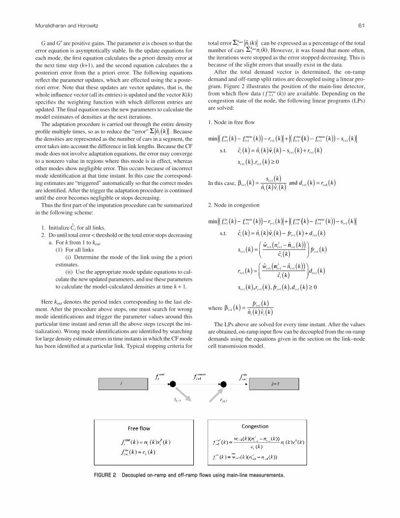
After the total demand vector is determined, the on-rampdemand and off-ramp split ratios are decoupled using a linear pro-gram. Figure 2 illustrates the position of the main-line detector,from which flow data ( f meas

i+1 (k)) are available. Depending on thecongestion state of the node, the following linear programs (LPs)are solved:

1. Node in free flow

In this case,

2. Node in congestion

where

The LPs above are solved for every time instant. After the valuesare obtained, on-ramp input flow can be decoupled from the on-rampdemands using the equations given in the section on the link–nodecell transmission model.

βii

i i

kfr k

n k v k++( ) =

( )( ) ( )1

1

ˆ ˆ

min f k f k r k f ki i i i+ + + +( ) − ( )( ) − ( ) +1 1 1 1in meas out (( ) − ( )( ) − ( )

( ) = ( )+ +f k s k

c k n k

i i

i i

1 1meas

s.t. ˆ ˆ vv k fr k d k

s kw n

i i i

i

i iJ

( ) − ( ) + ( )

( ) =−

+ +

++ +

1 1

11 1

ˆ nn k

c kfr k

r kw

i

ii

i

i

++

++

( )( )( )

⎛

⎝⎜⎞

⎠⎟( )

( ) =

11

11

ˆ

ˆ nn n k

c kd k

s k

iJ

i

ii

i

+ ++

+

− ( )( )( )

⎛

⎝⎜⎞

⎠⎟( )

( )

1 11

1

ˆ

ˆ

,, , ,r k fr k d ki i i+ + +( ) ( ) ( ) ≥1 1 1 0

βii

i ii ik

s k

n k v kd k r+

++ +( ) =

( )( ) ( ) ( ) =1

11ˆ ˆ

and 11 k( )

min f k f k r k f ki i i i+ + + +( ) − ( )( ) − ( ) +1 1 1 1in meas out (( ) − ( )( ) − ( )

( ) = ( )+ +f k s k

c k n k

i i

i i

1 1meas

s.t. ˆ ˆ vv k s k r k

s k r k

i i i

i i

( ) − ( ) + ( )( ) ( ) ≥

+ +

+ +

1 1

1 1 0,

Σ1k

in kend ( )Σ1

kin kend � ( )

FIGURE 2 Decoupled on-ramp and off-ramp flows using main-line measurements.

62 Transportation Research Record 2099

(a) (b)

0

5

10

700

600

500

400

300

200

100

0

Tim

e [h

r]

15

20

30 35 40

PostMile

45 50

PostMile

0

5

10

700

600

500

400

300

200

100

Tim

e [h

r]

15

20

30 35 40 45 50

FIGURE 3 Final density contours obtained after imputation.

(a) (b)

0

5

10

30

45

60

Tim

e [h

r]

15

20

30 35 40

PostMile

45 50

0

5

10

30

45

60

Tim

e [h

r]

15

20

30 35 40

PostMile

45 50

FIGURE 4 Velocity contours (in mph) obtained from I-210E simulation using imputed parameters.

APPLICATION

This section illustrates the application of the imputation algorithmto determine the on-ramp and off-ramp flow measurements in a26-mi-long section of the I-210E freeway in Pasadena. In this case,the freeway was divided into 26 links. Of a total of 30 on-ramps and21 off-ramps, seven on-ramps and five off-ramps had missing datafor the whole day. In addition, two on-ramps were identified to haveincorrect data. Presently incorrect ramp detector data are identifiedwith ad hoc rules—such as flow conservation along the node connect-ing the ramp detector stations/flow conservation along the main line(for the measured data). The imputation procedure was carried out forthese ramps. The fundamental diagram parameters for the links wereobtained from an automated calibration procedure described in Dervi-soglu et al. (5). The final density error in the imputation was reducedto 2.63%. Figure 3 shows that the density estimates have convergedto their true values without appreciable error.

A simulation was performed with the imputed data. For that pur-pose, calibrated fundamental diagram parameters and on-ramp flowsand off-ramp split ratios were specified for the freeway model. Thesimulation was performed using the Matlab implementation of the

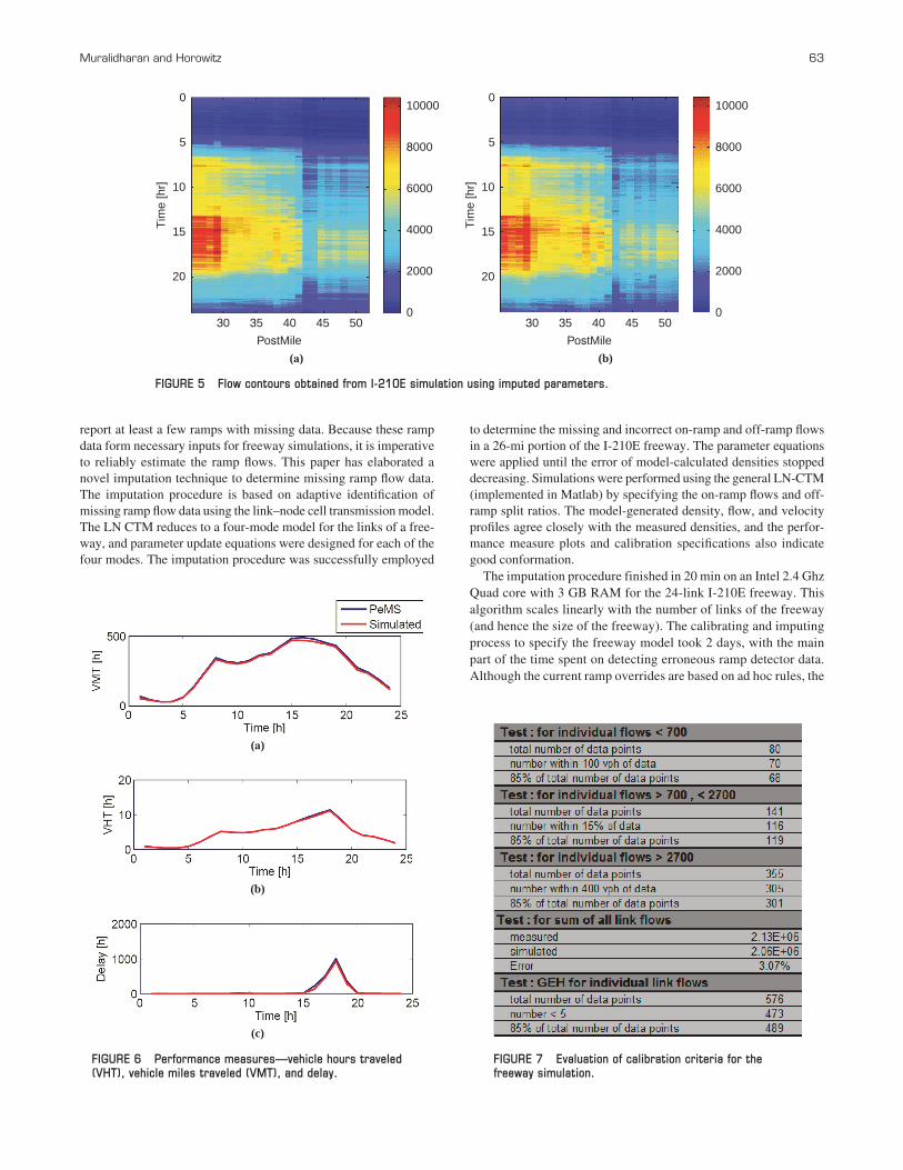
general LN-CTM used in Aurora (11). The simulation computesthe flow, density, and velocity profiles at each link for the giveninputs. Figure 4 shows the simulated and the measured velocity con-tours, and Figure 5 shows flow contours, both of which show goodagreement. The simulated contour plots clearly reproduce the loca-tions of the major bottlenecks. The simulated and measured per-formance measures are compared in Figure 6, and also show goodagreement. The simulated data had 2.63% and 3.58% density andflow errors, respectively. The flow error has been represented as apercentage of the total flow observed on the freeway. Finally, Fig-ure 7 lists the performance of the simulation as compared with thespecifications provided by the Wisconsin Department of Trans-portation (13). The simulation satisfies most of the requirements,while narrowly missing some of the criteria.

CONCLUSION

In California, although data are archived for main-line detectors rou-tinely, ramp detector data are often found to be entirely missing.Only a few freeways provide reliable on-ramp flows, and even these

Muralidharan and Horowitz 63

to determine the missing and incorrect on-ramp and off-ramp flowsin a 26-mi portion of the I-210E freeway. The parameter equationswere applied until the error of model-calculated densities stoppeddecreasing. Simulations were performed using the general LN-CTM(implemented in Matlab) by specifying the on-ramp flows and off-ramp split ratios. The model-generated density, flow, and velocityprofiles agree closely with the measured densities, and the perfor-mance measure plots and calibration specifications also indicategood conformation.

The imputation procedure finished in 20 min on an Intel 2.4 GhzQuad core with 3 GB RAM for the 24-link I-210E freeway. Thisalgorithm scales linearly with the number of links of the freeway(and hence the size of the freeway). The calibrating and imputingprocess to specify the freeway model took 2 days, with the mainpart of the time spent on detecting erroneous ramp detector data.Although the current ramp overrides are based on ad hoc rules, the

(a)

0

5

10

10000

8000

6000

4000

2000

0

Tim

e [h

r]

15

20

30 35 40

PostMile

45 50

(b)

0

5

10

10000

8000

6000

4000

2000

0

Tim

e [h

r]

15

20

30 35 40

PostMile

45 50

FIGURE 5 Flow contours obtained from I-210E simulation using imputed parameters.

(a)

(b)

(c)

FIGURE 6 Performance measures—vehicle hours traveled(VHT), vehicle miles traveled (VMT), and delay.

FIGURE 7 Evaluation of calibration criteria for thefreeway simulation.

report at least a few ramps with missing data. Because these rampdata form necessary inputs for freeway simulations, it is imperativeto reliably estimate the ramp flows. This paper has elaborated anovel imputation technique to determine missing ramp flow data.The imputation procedure is based on adaptive identification ofmissing ramp flow data using the link–node cell transmission model.The LN CTM reduces to a four-mode model for the links of a free-way, and parameter update equations were designed for each of thefour modes. The imputation procedure was successfully employed

authors are working toward a reliable fault detection model todetermine erroneous detector data to complement the imputationalgorithm.

ACKNOWLEDGMENT

Thisworkis supported by the California Department of Transportationthrough the California PATH Program.

REFERENCES

1. California Department of Transportation. Strategic Growth Plan. 2006.www.dot.ca.gov/docs/strategicgrowth.pdf. Accessed March 14, 2009.

2. California Center for Innovative Transportation. Corridor ManagementPlan Demonstration: Final Report. University of California, Berkeley,2006. www.calccit.org/resources/2007PDF/CCITTO3FinalReport-Jan5-07.pdf. Accessed March 14, 2009.

3. PeMS. PeMS website. 2007. pems.eecs.berkeley.edu. Accessed March14, 2009.

4. Daganzo, C. The Cell Transmission Model: A Dynamic Representationof Highway Traffic Consistent with the Hydrodynamic Theory. Trans-portation Research Part B, Vol. 28, No. 4, 1994, pp. 269–287.

5. Dervisoglu, G., G. Gomes, J. Kwon, R. Horowitz, and P. P. Varaiya.Automatic Calibration of the Fundamental Diagram and Empirical Obser-vations on Capacity. Presented at 88th Annual Meeting of the Transporta-tion Research Board, Washington, D.C., 2009.

64 Transportation Research Record 2099

6. Jacobson, L. N., N. L. Nihan, and J. D. Bender. Detecting ErroneousLoop Detector Data in a Freeway Traffic Management System. InTransportation Research Record 1287, TRB, National Research Council,Washington, D.C., 1990, pp. 151–166.

7. Dailey, D. Improved Error Detection for Inductive Loop Sensors.Technical Report WA-RD 3001. Washington State Department ofTransportation, 1993.

8. Chen, C., J. Kwon, J. Rice, A. Skabardonis, and P. Varaiya. DetectingErrors and Imputing Missing Data for Single-Loop Surveillance Sys-tems. In Transportation Research Record: Journal of the TransportationResearch Board, No. 1855, Transportation Research Board of NationalAcademies, Washington, D.C., 2003, pp. 160–167.

9. Messner, W., R. Horowitz, W.-W. Kao, and M. Boals. A New AdaptiveLearning Rule. IEEE Transactions on Automatic Control, Vol. 36, No. 2,1991, pp. 188–197.

10. Horowitz, R., W. Messner, and J. B. Moore. Exponential Convergenceof a Learning Controller for Robot Manipulators. IEEE Transactions onAutomatic Control, Vol. 36, No. 7, 1991, pp. 890–892.

11. Kurzhanskiy, A. Modeling and Software Tools for Freeway OperationalPlanning. PhD thesis. University of California, Berkeley, 2007.

12. Gomes, G., and R. Horowitz. Optimal Freeway Ramp Metering Usingthe Asymmetric Cell Transmission Model. Transportation ResearchPart C, Vol. 14, No. 4, 2006, pp. 244–262.

13. Wisconsin Department of Transportation. Freeway System OperationalAssessment: Paramics Calibration and Validation. Technical report.District 2, Milwaukee, 2002.

The contents of this paper reflect the views of the authors and not necessarilythe official views or policy of the California Department of Transportation.

The Traffic Flow Theory and Characteristics Committee sponsored publication ofthis paper.