Impurity Resistivity of fcc and hcp Fe-Based Alloys ...

ORIGINAL RESEARCHpublished: 29 November 2018doi: 10.3389/feart.2018.00217

Frontiers in Earth Science | www.frontiersin.org 1 November 2018 | Volume 6 | Article 217

Edited by:

Takashi Nakagawa,

University of Hong Kong, Hong Kong

Reviewed by:

Monica Pozzo,

University College London,

United Kingdom

Shin-ichi Takehiro,

Kyoto University, Japan

*Correspondence:

Hitoshi Gomi

[email protected]

Specialty section:

This article was submitted to

Geomagnetism and Paleomagnetism,

a section of the journal

Frontiers in Earth Science

Received: 31 May 2018

Accepted: 07 November 2018

Published: 29 November 2018

Citation:

Gomi H and Yoshino T (2018) Impurity

Resistivity of fcc and hcp Fe-Based

Alloys: Thermal Stratification at the

Top of the Core of Super-Earths.

Front. Earth Sci. 6:217.

doi: 10.3389/feart.2018.00217

Impurity Resistivity of fcc and hcpFe-Based Alloys: ThermalStratification at the Top of the Coreof Super-EarthsHitoshi Gomi* and Takashi Yoshino

Institute for Planetary Materials, Okayama University, Tottori, Japan

It is widely known that the Earth’s Fe dominant core contains a certain amount oflight elements such as H, C, N, O, Si, and S. We report the results of first-principlescalculations on the band structure and the impurity resistivity of substitutionallydisordered hcp and fcc Fe based alloys. The calculation was conducted by usingthe AkaiKKR (machikaneyama) package, which employed the Korringa-Kohn-Rostoker(KKR) method with the atomic sphere approximation (ASA). The local densityapproximation (LDA) was adopted for the exchange-correlation potential. The coherentpotential approximation (CPA) was used to treat substitutional disorder effect. Theimpurity resistivity is calculated from the Kubo-Greenwood formula with the vertexcorrection. In dilute alloys with 1 at. % impurity concentration, calculated impurityresistivities of C, N, O, S are comparable to that of Si. On the other hand, in concentratedalloys up to 30 at. %, Si impurity resistivity is the highest followed by C impurity resistivity.Ni impurity resistivity is the smallest. N, O, and S impurity resistivities lie between Si and Ni.Impurity resistivities of hcp-based alloys show systematically higher values than fcc alloys.We also calculated the electronic specific heat from the density of states (DOS). For pureFe, the results show the deviation from the Sommerfeld value at high temperature, whichis consistent with previous calculation. However, the degree of deviation becomes smallerwith increasing impurity concentration. The violation of the Sommerfeld expansion isone of the possible sources of the violation of the Wiedemann-Franz law, but thepresent results could not resolve the inconsistency between recent electrical resistivityand thermal conductivity measurements. Based on the present thermal conductivitymodel, we calculated the conductive heat flux at the top of terrestrial cores, which iscomparable to the heat flux across the thermal boundary layer at the bottom of themantle. This indicates that the thermal stratification may develop at the top of the liquidcore of super-Earths, and hence, chemical buoyancies associated with the inner coregrowth and/or precipitations are required to generate the global magnetic field throughthe geodynamo.

Keywords: band structure, density of states, electrical resistivity, thermal conductivity, Linde’s rule, KKR-CPA

https://www.frontiersin.org/journals/earth-science

https://www.frontiersin.org/journals/earth-science#editorial-board




https://doi.org/10.3389/feart.2018.00217

http://crossmark.crossref.org/dialog/?doi=10.3389/feart.2018.00217&domain=pdf&date_stamp=2018-11-29


https://www.frontiersin.org

https://www.frontiersin.org/journals/earth-science#articles

https://creativecommons.org/licenses/by/4.0/

mailto:[email protected]

https://doi.org/10.3389/feart.2018.00217

https://www.frontiersin.org/articles/10.3389/feart.2018.00217/full

http://loop.frontiersin.org/people/521528/overview

Gomi and Yoshino Impurity Resistivity of Fe Alloys

INTRODUCTION

Because the electrical current and the heat are mainly transportedby mobile electrons in the metallic core, it is important tounderstand the electron scattering mechanisms in Fe-basedalloys at high pressure and temperature to estimate the thermalconductivity and the electrical resistivity. Gomi et al. (2013)proposed the core resistivity model that the resistivity saturationwas firstly taken into account. Later, many studies (Kiarasi andSecco, 2015; Gomi et al., 2016; Ohta et al., 2016, 2018; Pozzo andAlfè, 2016a,b; Wagle et al., 2018; Xu et al., 2018) investigatedthe resistivity saturation. Because of its universality, we expectthat the resistivity saturation model is applicable to metalliccores of terrestrial planets with various pressure, temperatureand compositions. In order to improve our previous model, weaddress the following two topics in this study.

The first topic of this study is the compositional effect onthe electrical resistivity of cores, namely impurity resistivity.On the one hand, first-principles molecular dynamics (FPMD)studies computed the effects of alloying Si, O, and S (de Kokeret al., 2012; Pozzo et al., 2013, 2014; Wagle et al., 2018). Onthe other hand, high pressure experimental works investigatedthe impurity resistivities of Si, Ni, S and C (Matassov, 1977;Gomi et al., 2013, 2016; Seagle et al., 2013; Gomi and Hirose,2015; Kiarasi and Secco, 2015; Suehiro et al., 2017; Ohta et al.,2018; Zhang et al., 2018). In order to understand the relativeimportance of light elements, Gomi et al. (2013) calculated theimpurity resistivities of C, S, and O from the impurity resistivityof silicon by using the Linde’s rule (Norbury, 1921; Linde, 1932).However, Suehiro et al. (2017) demonstrated the violation ofthe Linde’s rule from measurements on Fe-Si-S ternary alloys.The Linde’s rule is known as a model for impurity resistivity innoble metal hosts, which predicts a parabolic dependence as afunction of valence difference Z between impurity element andthe host metal. The Linde’s rule is valid for impurity elementslocated at the right hand side of the host noble metal in theperiodic table, however, it is strongly violated for magnetictransition metal impurity. Therefore, application to transitionmetal hosts is indeed questionable. Instead of the Linde’s rule,we will show the relative importance of the impurity resistivityof light alloying elements in fcc and hcp Fe by means of theKorringa-Kohn-Rostoker method combined with the coherentpotential approximation (KKR-CPA) (Oshita et al., 2009; Kouand Akai, 2018), which successfully reproduces the impurityresistivities of Si and Ni in hcp Fe (Gomi et al., 2016).

The second topic of this study is the validity of theWidemann-Franz law. The Widemann-Franz law predicts the thermalconductivity from the electrical resistivity as:

k =LT

ρ(1)

where k is the thermal conductivity, L is the Lorenz number,T is the absolute temperature and ρ is the electrical resistivity.The Lorenz number is almost independent of temperatureand common for almost all metals. The Sommerfeld valueLSomm = 1

3π2k2Be2

= 2.445 × 10−8 W�/K2 is widely

used as the Lorenz number, where kB is the Boltzmann’sconstant and e is electronic charge (e.g., Anderson, 1998;Poirier, 2000; see also Appendix of Gomi and Hirose, 2015).However, FPMD studies predict the deviation of the Lorenznumber from the Sommerfeld value (de Koker et al., 2012;Pozzo et al., 2012, 2013, 2014; Pozzo and Alfè, 2016b). Moreimportantly, the experimentally determined Lorenz numberof hcp Fe, which is calculated from recent laser heateddiamond-anvil cell (LHDAC) measurements on the electricalresistivity (Ohta et al., 2016) and the thermal conductivity(Konôpková et al., 2016), exhibit substantially smaller than theSommerfeld value. Even though these LHDAC results may havelarge uncertainty (Dobson, 2016), this fact suggests potentialviolation of the Widemann-Franz law. Gomi and Hirose (2015)pointed out three important approximations, which potentiallyviolate the Wiedemann-Franz law: omitting the additionalcontribution from lattice or ionic conductivity, neglecting theanelastic scattering, and the application of the Sommerfeldexpansion. Additionally, electron-electron scattering may affectthe Lorenz number (Pourovskii et al., 2017). Among them,the violation of the Sommerfeld expansion may cause 2–43% deviation from the Sommerfeld value of the Lorenznumber, if we adopt the calculated electron density of states(DOS) of fcc and hcp Fe reported by Boness et al. (1986).However, this argument is limited to pure Fe. As well as theimpurity resistivity calculation, the KKR-CPA method can easilysimulate the DOS of disordered alloys (Gomi et al., 2016,2018).

This paper is organized as follows. In the section Methods,the first-principles methods were described. The impurityresistivities of various impurities in fcc Au were first calculatedto examine the validity and the physical origin of the violationof the Linde’s rule (section Dilute Alloys). Then, impurityresistivities in fcc and hcp Fe-based alloys were simulatedat high pressure (sections Dilute Alloys and ConcentratedAlloys). Simultaneously, electron DOS were computed. Theelectronic specific heat was then estimated by numericalintegration based on the DOS. The numerically-calculatedspecific heat values were compared with that was obtained bythe Sommerfeld expansion to discuss the possible deviationof the Lorenz number from its Sommerfeld value (sectionElectronic Specific Heat andWiedemann-Franz Law). Combinedwith the present impurity resistivity and the Lorenz number,we revised our thermal conductivity model (Gomi et al.,2016) (section Electrical Resistivity and Thermal Conductivityof the Earth’s Core). Finally, the model was applied to theplanetary cores with various planetary mass from 0.1 to 10times Earth mass (section Heat Flux at the CMB of Super-Earths).

METHODS

We carried out the first-principles electronic band structurecalculation of fcc Au-, hcp and fcc Fe-based alloys. For fcc Aualloys, the lattice parameters are set to a = 7.71 Bohr, whichcorrespond the ambient pressure value. For hcp Fe alloys, the






lattice volumes are set to 19.10, 16.27, and 9.80 Å3. Thesevalues correspond to 40, 120, and 1,000 GPa pressure at ambienttemperature (Dewaele et al., 2006). The axial ratio was set to theideal value (c/a = 1.633). For fcc Fe alloys, we used the sameatomic volumes as for hcp Fe alloys. The Kohn-Sham equationwas solved by means of Korringa-Kohn-Rostoker (KKR) Greenfunction method, which implemented in AkaiKKR package(Akai, 1989). The local density approximation (LDA) wasadapted to exchange-correlation potential (Moruzzi et al., 1978);the specific choice of the exchange-correlation functional maynot significantly affect the resistivity value (see SupplementaryFigure S1 of Gomi et al., 2016). The crystal potential wasapproximated by using the atomic spherical approximation(ASA). The maximum angular momentum quantum numberwas set to l = 3. Relativistic effects are considered in thescalar relativistic approximation. The substitutional chemicaldisorder is described in the coherent potential approximation(CPA). The electrical resistivity is calculated from the Kubo-Greenwood formula with the vertex correction (Butler, 1985;Oshita et al., 2009; Gomi et al., 2016; Kou and Akai, 2018).The hcp Fe-alloys have two independent resistivity componentswith respect to crystallographic orientation; ρ|| and ρ⊥ arethe resistivities calculated parallel and perpendicular to the c-axis, respectively. The resistivities of polycrystalline hcp Fe-alloys are calculated as ρpoly = (2ρ⊥ +ρ||)/3 (Alstad et al.,1961).

DILUTE ALLOYS

Norbury (1921) conducted systematic measurements of impurityresistivity of dilute alloys, and found that the impurityresistivity is enhanced with increasing horizontal distancebetween the positions of impurity element and host metalin the periodic table. Linde (1932) reported that impurityresistivity of noble metal-based alloys is proportional toZ2, where Z is the difference in valence between impurityelement and host metal. This relationship is observed in thenoble metal alloyed with the impurity element located at theright hand side of the noble metal in the periodic table,and is so-called the Linde’s rule. Mott (1936) provided aninterpretation for Linde’s rule, assuming the impurity atomto be a point charge Z × e, where e is the elementaryelectrical charge. This approximation successfully explained theZ2 dependence of the impurity resistivity. However, impurityelements on the left hand side of the noble metal exhibitcomplicated behavior. This is reasonably explained by Friedelmodel with the idea of the virtual bond state (VBS) (Friedel,1956).

Figure 1A shows the impurity resistivities of impurityelements with the atomic numbers from 1 (H) to 18 (Kr) in fccAu host. We tried to simulate both of non-magnetic and localmagnetic disorder (LMD) state for all these impurity elements,and the LMD solution was obtained only for V, Cr, Mn, Fe, Co,and Ni impurity. For these six impurity elements, the impurityresistivity value is largely different between the non-magneticstate and the LMD state, and the LMD results are consistent with

FIGURE 1 | Impurity resistivities of 1st (green cross; H and He), 2nd (bluediamond; Li, Be, B, C, N, O, F and Ne), 3rd (orange triangle; Na, Mg, Al, Si, P,S, Cl, and Ar) and 4th (black square; K, Ca, Sc, Ti, V, Cr, Mn, Fe, Co, Ni, Cu,Zn, Ga, Ge, As, Se, Br and Kr) period elements. (A) fcc Au-alloys at 1 barcompared with literature values (Friedel, 1956). (B) hcp Fe-alloys at 40 GPacompared with previous DAC experiments (Ni: Gomi and Hirose, 2015; Si:Gomi et al., 2016; C: Zhang et al., 2018). (C) fcc Fe-alloys at 40 GPa. Incommon, solid symbols with solid lines are present nonmagnetic calculations,gray square symbols with broken line are obtained from present LMDcalculations and open symbols represent previous experiments.

previous experimental results. The impurity resistivities of theother 12 elements without local magnetic moments show goodagreement with previous experimental results (Friedel, 1956).






For 3rd period impurity elements located at the right handside of Cu in the periodic table, namely Zn, Ga, Ge and As, areknown to follow the Linde’s rule (Norbury, 1921; Linde, 1932),and our first-principles calculations without local magneticmoment well reproduce previous experimental results (Friedel,1956). Our calculations on 13 to 15 group of 2nd and 3rd periodelements, which include the possible candidates of the lightelements alloying with planetary cores (C, N, O, Si, S), also showthe similar trend predicted by the Linde’s rule.

In the Figure 1A, filled squares are present first-principlescalculation without spin-polarization, which show paraboladependence. Open squares indicate present first-principles withlocal magnetic disorder (LMD), which reproduce previousexperimental results (Friedel, 1956). To discuss the Friedelmode, we computed the partial density of states (PDOS) ofimpurity elements in fcc Au (Figure 2). Figure 2A shows thenon-magnetic PDOS of Ti, V, Cr, Mn, Fe, Co, and Ni. Infcc Au, PDOS of these transition impurities have a sharppeak at the vicinity of the Fermi level, which is so-calledvirtual bond state (VBS) (Friedel, 1956; Mertig, 1999). Thepeak position shifts from high energy to low energy withincreasing the atomic number. The impurity resistivities of non-magnetic fcc Au-based alloys exhibit the maximum coincidencewith the VBS peak across the Fermi energy. Experimental andLMD impurity resistivity can also be explained by the peakposition relevant to the Fermi energy. Figure 2B representsthe PDOS of Cr with non-magnetic (solid line) and LMD(broken lines). The impurity resistivity of non-magnetic Cris predicted to be 1.0 × 10−7 �m, which is larger thanthe experimental value of 4.0 × 10−8 �m. In an oppositemanner, non-magnetic Co impurity resistivity is larger thanexperimental and LMD impurity resistivity. The VBS of non-magnetic Co is a little bit shifted to lower energy comparedwith the Fermi energy, but, in LMD state, the VBS split and theup spin peak move to the Fermi level. This causes the strongscattering.

Figure 1B shows the impurity resistivities of hcp Fe-basedalloys at the volume of 19.1 Å3, which corresponds to the pressureof 40 GPa for pure hcp Fe at 300K (Dewaele et al., 2006).Experimentally determined impurity resistivities of Ni, Si, andC are also plotted, which is interpolated between binary alloys(Gomi and Hirose, 2015; Gomi et al., 2016; Zhang et al., 2018)and pure Fe (Gomi et al., 2013) at ambient temperature. Thepresent calculations of impurity resistivities of light elementcandidates (C, N, O, Si, and S) are almost identical and largerthan Ni impurity resistivity. It is well-known that the impurityresistivity of 3d transition metal impurity in 3d transition metalhost is small, in general (Tsiovkin et al., 2005, 2006). Amongthe light element candidates, the impurity resistivity increaseswith increasing atomic number in the same period. Also, inthe same group, the second period atoms show higher impurityresistivity than third period atoms, which is consistent with theexperimental fact that the impurity resistivity of C (Zhang et al.,2018) is higher than that of Si (Gomi et al., 2016). This trendis also observed for fcc Fe-based alloys (Figure 1C). Impurityresistivity of H seems comparable to the other light elements,however, it may be overestimate. In this study, we assumed that

FIGURE 2 | Partial density of states (PDOS) of impurity elements in fcc Au.(A) PDOS of Ti (purple), V (green), Cr (cyan), Mn (orange), Fe (yellow), Co(blue), and Ni (red) without local magnetic moment. (B) PDOS of Cr with(broken lines) and without (solid line) local magnetic moment. (C) PDOS of Cowith (broken line) and without (solid line) local magnetic moment.

the all impurity elements substitute the Fe sites. But H is knownto enter the interstitial sites (Antonov et al., 2002; Fukai, 2006).The partial density of states (PDOS) of interstitial H in hcpand double hexagonal close-packed (dhcp) Fe is located at farbelow the Fermi energy (e.g., Tsumuraya et al., 2012; Gomi et al.,2018). Therefore, Gomi et al. (2018) argued that the impurityresistivity of interstitial hydrogen is negligibly small. This isconsistent with recent DAC experiments on fcc FeHx alloys(Ohta et al., 2018).






CONCENTRATED ALLOYS

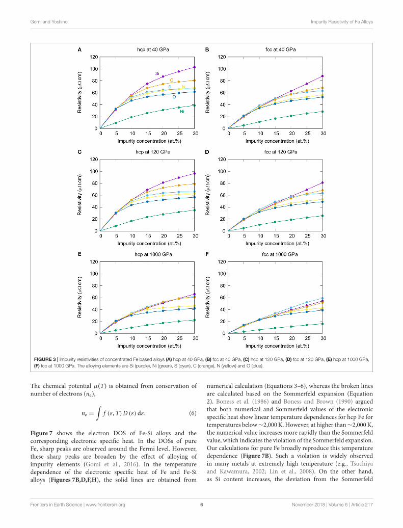
In the previous section, we discussed dilute alloys, however, theEarth’s core should have a large amount of impurity elements(e.g., Hirose et al., 2013). Gomi et al. (2016) reported theresistivity calculation of Fe-Si and Fe-Ni alloys by using the KKR-CPA method, as well as DAC experiments of Fe-Si alloys. Here,we show the systematic survey of impurity resistivity of lightelement candidates (C, N, O, Si, and S) and Ni in Fe-basedhigh concentration alloys at zero Kelvin (Figure 3 and Table 1).Basically, impurity resistivity of light element candidates islarger than Ni, which agree with dilute alloy results. This canqualitatively be understood in terms of the broadening of energydispersion via the uncertainty relationship between energy andtime; 1E1t ≥ h/2, where 1E is the uncertainty in energy, 1tis electron life time, and h is the reduced Planck’s constant(the Dirac’s constant) (Gomi et al., 2016). Figure 4 shows theBloch spectral function along with the path, which connects thehigh symmetry points in the Brillouin zone of the hexagonallattice. If there is no scattering, the Bloch spectral function isequivalent to the band structure of perfectly ordered crystal.Indeed, the broadening features of Fe-Ni alloys are weakerthan that of other Fe-light elements alloys. At 19.10 Å3 (∼40GPa), Si shows the largest impurity resistivity, followed by C,S, and N. The smallest impurity resistivity is obtained from Oimpurity among the light element candidates. Note that thissequential order is completely different from that of dilute alloys(Figure 1).

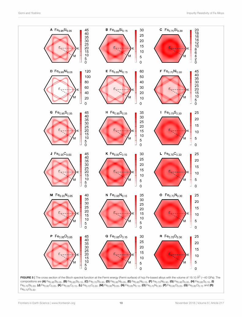
This is potentially explained by the variation of the saturationresistivity due to the chemical composition. The electricalresistivity of transition metals and alloys tends to saturate at highresistivity (Mooij, 1973; Bohnenkamp et al., 2002). This resistivitysaturation is observed when the mean free path of conductionelectrons becomes comparable to the inter-atomic distance; thiscondition is so-called the Mott-Ioffe-Regel criteria (Mott, 1972;Gurvitch, 1981). This condition may be graphically identifiedfrom the cross sections of the Bloch spectral function at the Fermienergy (Figure 5), because the inverse of the mean free path isproportional to the width of the Fermi surface broadening, andthe boundary of the first Brillouin zone is proportional to theinverse of the lattice parameter (Butler and Stocks, 1984; Butler,1985; Banhart et al., 1989; Glasbrenner et al., 2014; Gomi et al.,2016). Gomi et al. (2016) compared the cross section of Fe-Siand Fe-Ni alloys, and argued that the non-linear concentration-resistivity relationship observed in Fe-Ni alloys is explained bythe Nordheim’s rule, whereas that of Fe-Si alloys is due to theresistivity saturation. Interestingly, the broadening feature of S,C, N and O impurity alloys are similar to the Si alloy. Especially,the O alloy’s width seems even larger than that of Si alloy. Thissuggests that the high-concentration Fe-O alloys satisfies theMott-Ioffe-Regel criteria, even though the impurity resistivity issmaller than Fe-Si alloy.

We also calculated the impurity resistivity of Fe-Si-S ternaryalloys (Figure 6). The results are consistent with the DACmeasurements by Suehiro et al. (2017). Figure 6 also impliesthe violation of the Matthiessen’s rule, which is a simple sumrule of resistivity of all the scattering terms. The violation of the

Matthiessen’s rule is already reported by previous calculations(Glasbrenner et al., 2014; Gomi et al., 2016; Drchal et al., 2017).

ELECTRONIC SPECIFIC HEAT ANDWIEDEMANN-FRANZ LAW

Only a few direct thermal conductivity measurements at highpressure and temperature have been reported (Konôpková et al.,2011, 2016; McWilliams et al., 2015). Even though the thermalconductivity can directly be calculated from first-principlescalculations (Sha and Cohen, 2011; de Koker et al., 2012; Pozzoet al., 2012, 2013, 2014; Pozzo and Alfè, 2016b; Pourovskii et al.,2017; Wagle et al., 2018; Xu et al., 2018; Yue and Hu, 2018),the Wiedemann-Franz law has been widely used to estimatethe thermal conductivity of the Earth’s core from the electricalresistivity measurements (Anderson, 1998; Stacey and Anderson,2001; Stacey and Loper, 2007; Deng et al., 2013; Gomi et al., 2013,2016; Seagle et al., 2013; Gomi and Hirose, 2015; Ohta et al.,2016, 2018; Hieu et al., 2017; Suehiro et al., 2017; Pommier, 2018;Silber et al., 2018; Zhang et al., 2018) (see Williams, 2018 for arecent review). The Lorenz number is related to the electronicband structure (Vafayi et al., 2006; Gomi and Hirose, 2015;Secco, 2017). Gomi and Hirose (2015) mentioned that the Lorenznumber may have up to ∼40 % uncertainty, based on the first-principles calculations on the electronic specific heat reportedby Boness et al. (1986). However, this value was calculated onlyfor pure Fe. Therefore, in this section, we investigated how thespecific heat deviates from its Sommerfeld value for Fe-basedalloys.

At around the ambient temperature, the electronic specificheat can be estimated based on the Sommerfeld expansion,

cve (T) =π2

3k2BD(εF)T (2)

where cve is the electronic specific heat, kB is the Boltzmannconstant, εF is the Fermi energy, D(ε) is the DOS, andT is temperature. However, this relation is violated at hightemperatures, as in terrestrial planetary cores (Boness et al., 1986;Boness and Brown, 1990; Tsuchiya and Kawamura, 2002; Linet al., 2008). The exact values can be calculated from numericalintegration with the electronic density of state. Following Bonesset al. (1986), we calculated the electronic specific heat from itsdefinition:

cve (T) =

(

∂ue

∂T

)

v

, (3)

where ue is the internal energy of electrons, which can beobtained from electron density of state D(ε),

ue (T) =

∫

εf (ε,T)D (ε) dε (4)

and f (ε, T) is the Fermi-Dirac distribution function,

f (ε,T) =1

exp{

ǫ−µ(T)kBT

}

+ 1. (5)






FIGURE 3 | Impurity resistivities of concentrated Fe based alloys (A) hcp at 40 GPa, (B) fcc at 40 GPa, (C) hcp at 120 GPa, (D) fcc at 120 GPa, (E) hcp at 1000 GPa,(F) fcc at 1000 GPa. The alloying elements are Si (purple), Ni (green), S (cyan), C (orange), N (yellow) and O (blue).

The chemical potential µ(T) is obtained from conservation ofnumber of electrons (ne),

ne =

∫

f (ε,T)D (ε) dε. (6)

Figure 7 shows the electron DOS of Fe-Si alloys and thecorresponding electronic specific heat. In the DOSs of pureFe, sharp peaks are observed around the Fermi level. However,these sharp peaks are broaden by the effect of alloying ofimpurity elements (Gomi et al., 2016). In the temperaturedependence of the electronic specific heat of Fe and Fe-Sialloys (Figures 7B,D,F,H), the solid lines are obtained from

numerical calculation (Equations 3–6), whereas the broken linesare calculated based on the Sommerfeld expansion (Equation2). Boness et al. (1986) and Boness and Brown (1990) arguedthat both numerical and Sommerfeld values of the electronicspecific heat show linear temperature dependences for hcp Fe fortemperatures below∼2,000K. However, at higher than∼2,000K,the numerical value increases more rapidly than the Sommerfeldvalue, which indicates the violation of the Sommerfeld expansion.Our calculations for pure Fe broadly reproduce this temperaturedependence (Figure 7B). Such a violation is widely observedin many metals at extremely high temperature (e.g., Tsuchiyaand Kawamura, 2002; Lin et al., 2008). On the other hand,as Si content increases, the deviation from the Sommerfeld






expansion becomes small (Figure 7). This trend is also foundin other Fe-light element alloys. Boness et al. (1986) arguedthat the relation between the deviation and the location ofthe Fermi level is within the sharp peaks of the DOS. Inthis sense, in highly concentrated alloys, these sharp peaksare smeared out because of impurity scattering. This is thereason why the deviation from the Sommerfeld expansion isrelatively small in highly concentrated alloys. The Wiedemann-Franz law is based on the fact that the carrier of both of electriccurrent and heat is conduction electrons. The pre-factor oflinear temperature dependence attributed to the result of theSommerfeld expansion, thus, Gomi and Hirose (2015) pointedout the deviation of the Lorenz number from its Sommerfeldvalue.

Figure 8 represents the deviation of the Lorenz numberof Fe alloyed with Ni or light element candidates as functionof temperature. The representative values at V = 16.27Å3 and T = 4,000K or 5,500K are summarized in theTable 2. Broadly speaking, Fe-Si alloys show relativelylarge Lorenz number, whereas the alloying O tend todecrease the Lorenz number. Also, the Lorenz numberdecreases with increasing impurity concentration and/ortemperature. These trends are consistent with previous first-principles molecular dynamics calculation (de Koker et al.,2012).

It is worth mentioning about the relationship between energy-dependent conductivity σ (ε) and the Lorenz number. Thethermal conductivity of metals is represented by using theOnsager’s kinetic coefficient,

Kn =

∫

σ (ε) (ε − µ)n(

−∂f

∂ε

)

dε, (7)

the electrical resistivity can be described as

σ = K0, (8)

and the thermal conductivity is

k =1

e2T

(

K2 −K21

K0

)

(9)

Applying the relaxation time approximation, the energy-dependent conductivity function can be expressed as

σ (ε) =e2

3D (ε) {v (ε)}2 τ (ε) (10)

where D(ε) is the density of states, v(ε) is the group velocityand τ (ε) is the relaxation-time. Pourovskii et al. (2017) focusedon the energy dependence of the relaxation-time of electron-electron scattering. They conducted the dynamical mean-field theory (DMFT) calculations to incorporate the electroncorrelation effects and found that the hcp Fe exhibits a nearlyperfect Fermi liquid (FL) behavior, which strongly decreasethe Lorenz number and hence the thermal conductivity. Xuet al. (2018) also carried out DMFT calculations. Althoughthey did not observe FL behavior at high temperature, the

TABLE 1 | Impurity resistivity of Fe-alloys at zero Kelvin.

χ (at.%) ρhcp,⊥(µ�cm)

ρhcp,||(µ�cm)

ρhcp,poly(µ�cm)

ρfcc(µ�cm)

Fe-Si ALLOYS AT V = 9.55 Å3/ATOM (P∼40 GPa).

5 29.11 37.40 31.87 19.47

10 50.85 67.75 56.49 36.25

15 67.70 89.84 75.08 50.24

20 79.95 101.67 87.19 62.76

25 89.73 107.71 95.73 75.06

30 98.45 111.69 102.86 88.03

Fe-Ni ALLOYS

5 8.38 11.61 9.46 5.26

10 18.04 20.50 18.86 11.27

15 24.84 27.84 25.84 16.75

20 29.55 34.00 31.03 21.25

25 33.34 39.21 35.30 25.32

30 36.36 43.43 38.72 28.45

Fe-S ALLOYS

5 31.49 37.61 33.53 21.31

10 48.34 61.42 52.70 38.72

15 56.38 70.47 61.08 50.62

20 60.74 72.76 64.75 57.37

25 63.28 72.41 66.32 61.25

30 64.78 71.19 66.92 63.47

Fe-C ALLOYS

5 30.86 37.45 33.05 20.13

10 50.75 64.91 55.47 36.18

15 62.30 79.62 68.07 48.49

20 69.36 85.28 74.66 57.64

25 74.22 86.90 78.45 64.05

30 77.70 86.65 80.68 68.38

Fe-N ALLOYS

5 31.19 38.11 33.50 21.49

10 46.24 59.67 50.72 35.11

15 54.00 69.07 59.02 43.64

20 58.82 72.79 63.48 49.27

25 62.23 74.12 66.20 53.29

30 64.92 74.52 68.12 56.45

Fe-O ALLOYS

5 30.32 38.16 32.94 21.61

10 42.43 56.01 46.96 34.20

15 48.33 63.30 53.32 41.58

20 52.20 66.62 57.00 46.41

25 55.22 68.53 59.65 49.97

30 57.61 69.85 61.69 52.65

Fe-Si ALLOYS AT V = 8.14 Å3/ATOM (P ∼ 120 GPA).

5 26.82 34.58 29.41 18.22

10 46.62 62.39 51.88 33.59

15 62.08 82.74 68.97 46.44

20 74.07 94.98 81.04 57.92

25 83.55 101.32 89.47 69.12

30 91.98 105.30 96.42 81.03

(Continued)






TABLE 1 | Continued


ρhcp,||(µ�cm)

ρhcp,poly(µ�cm)

ρfcc(µ�cm)

Fe-Ni ALLOYS

5 7.79 9.39 8.33 4.70

10 16.87 16.27 16.67 10.49

15 22.00 25.76 23.25 14.98

20 26.49 30.66 27.88 18.75

25 30.01 35.26 31.76 22.48

30 32.70 39.17 34.86 25.47

Fe-S ALLOYS

5 28.88 34.75 30.83 19.52

10 46.10 58.91 50.37 36.04

15 54.75 69.09 59.53 49.10

20 59.49 72.01 63.66 57.15

25 62.24 71.80 65.43 61.32

30 63.87 70.34 66.03 63.30

Fe-C ALLOYS

5 28.60 35.28 30.82 18.63

10 47.58 61.48 52.22 33.43

15 59.42 76.96 65.27 45.27

20 66.91 83.75 72.52 54.99

25 71.97 85.86 76.60 62.62

30 75.54 85.79 78.95 68.20

Fe-N ALLOYS

5 29.59 30.56 29.92 19.99

10 44.10 56.67 48.29 33.21

15 51.22 65.48 55.97 41.39

20 55.21 68.22 59.54 46.65

25 57.88 68.77 61.51 50.34

30 59.92 68.56 62.80 53.16

Fe-O ALLOYS

5 28.61 33.23 30.15 20.20

10 39.67 51.43 43.59 31.85

15 44.77 58.07 49.20 38.69

20 48.15 61.04 52.44 43.23

25 50.79 62.67 54.75 46.57

30 53.02 63.83 56.62 49.19

Fe-Si ALLOYS AT V = 4.90 Å3/ATOM (P∼1,000 GPA).

5 17.83 20.32 18.66 12.24

10 30.13 36.60 32.29 22.49

15 39.60 48.54 42.58 31.36

20 47.84 57.28 50.98 39.29

25 55.60 64.51 58.57 46.80

30 63.12 71.51 65.92 54.36

Fe-Ni ALLOYS

5 4.87 5.38 5.04 2.98

10 9.48 10.18 9.71 6.21

15 13.60 14.67 13.95 8.92

20 16.66 18.79 17.37 11.46

25 19.14 22.27 20.19 14.00

30 21.29 25.03 22.53 16.10

(Continued)

TABLE 1 | Continued


ρhcp,||(µ�cm)

ρhcp,poly(µ�cm)

ρfcc(µ�cm)

Fe-S ALLOYS

5 19.03 21.11 19.72 12.88

10 31.78 38.30 33.95 23.85

15 41.40 51.35 44.72 33.72

20 48.72 60.63 52.69 43.18

25 53.94 66.41 58.09 52.23

30 58.19 69.22 61.87 58.84

Fe-C ALLOYS

5 19.11 21.10 19.77 12.43

10 31.05 37.05 33.05 22.27

15 40.35 49.32 43.34 30.34

20 48.49 61.30 52.76 37.55

25 51.74 71.76 58.42 44.55

30 54.73 72.70 60.72 51.64

Fe-N ALLOYS

5 20.48 22.30 21.08 13.31

10 31.37 37.34 33.36 23.45

15 37.51 46.04 40.35 31.00

20 39.96 49.63 43.18 36.42

25 41.96 50.92 44.95 40.18

30 44.01 51.44 46.48 42.79

Fe-O ALLOYS

5 20.15 22.56 20.95 14.03

10 28.10 34.64 30.28 22.95

15 32.20 40.61 35.00 28.80

20 35.03 43.81 37.96 33.03

25 37.44 45.78 40.22 36.26

30 39.58 47.14 42.10 38.77

energy dependence of the relaxation-time reduced the Lorenznumber by 20–45% of the Sommerfeld value. Yue and Hu(2018) calculated the thermal conductivity of hcp Fe based onthe non-equilibrium ab initio molecular dynamics (NEAIMD)simulation, which simultaneously incorporates the electron-phonon and electron-electron scattering. On the other hand,the present study focused on the energy dependence of theDOS, via the electronic specific heat, which also relates to theenergy dependent conductivity as Equation (10). These recenttheoretical assessments on the Lorenz number have been partlymotivated by the inconsistency of experimental results betweenthe electrical resistivity measurement by Ohta et al. (2016) andthe thermal conductivity measurements by Konôpková et al.(2016) (see also Dobson, 2016). The theoretical works are broadlyconsistent with the experimental result of low resistivity (Ohtaet al., 2016), however, failed to reproduce the low thermalconductivity (Konôpková et al., 2016). Pourovskii et al. (2017)reported k = 190 W/m/K for hcp Fe at the inner core boundary(ICB) condition. Xu et al. (2018) suggested k = 97 W/m/Kfor hcp Fe at the CMB. Yue and Hu (2018) obtained k ∼ 190W/m/K for hcp Fe at both of the CMB and ICB. These valuesare significantly higher than k = 33 and 46 W/m/K at the CMB






FIGURE 4 | The band structure of hcp Fe-based alloys with the volume of 19.10 Å3 (∼40 GPa). The Fermi energy is set to be 0 Ry. The compositions are (A)Fe0.95Si0.05, (B) Fe0.85Si0.15, (C) Fe0.70Si0.30, (D) Fe0.95Ni0.05, (E) Fe0.85Ni0.15, (F) Fe0.70Ni0.30, (G) Fe0.95S0.05, (H) Fe0.85S0.15, (I) Fe0.70Si0.30, (J)Fe0.95C0.05, (K) Fe0.85C0.15, (L) Fe0.70C0.30, (M) Fe0.95N0.05, (N) Fe0.85N0.15, (O) Fe0.70N0.30, (P) Fe0.95O0.05, (Q) Fe0.85O0.15 and (R) Fe0.70O0.30.






FIGURE 5 | The cross section of the Bloch spectral function at the Fermi energy (Fermi surface) of hcp Fe-based alloys with the volume of 19.10 Å3 (∼40 GPa). Thecompositions are (A) Fe0.95Si0.05, (B) Fe0.85Si0.15, (C) Fe0.70Si0.30, (D) Fe0.95Ni0.05, (E) Fe0.85Ni0.15, (F) Fe0.70Ni0.30, (G) Fe0.95S0.05, (H) Fe0.85S0.15, (I)Fe0.70Si0.30, (J) Fe0.95C0.05, (K) Fe0.85C0.15, (L) Fe0.70C0.30, (M) Fe0.95N0.05, (N) Fe0.85N0.15, (O) Fe0.70N0.30, (P) Fe0.95O0.05, (Q) Fe0.85O0.15 and (R)Fe0.70O0.30.






FIGURE 6 | Impurity resistivity of hcp Fe100−xSix binary (green) andFe95−xSixS5 ternary (purple) alloys as a function of silicon content at thevolume of 19.10 Å (∼40 GPa) and zero Kelvin. Gray broken line shows thesum of the resistivity of Fe95S5 and Fe100−xSix (the Matthiessen’s rule). Theorange cross represents the resistivity of hcp Fe89.3Si5.7S5.0 alloy measuredat ∼40 GPa and ambient temperature (Suehiro et al., 2017).

and ICB, respectively (Konôpková et al., 2016). This situation isnot altered by considering the effect of alloying on the energydependence of DOS obtained by this study, and the uncertaintiesdue to the deviation from the Sommerfeld value may be smaller

ρph,ideal (V ,T) = B (V)

(

T

2D (V)

)5 ∫ 2D(V)T

0

x5dx

(exp (x) − 1)(1− exp (−x))(14)

than 30% for the Earth’s core (see Table 2). Therefore, weconclude that, even though it is a not good approximation forpure Fe, the Sommerfeld value is a good proxy of the Lorenznumber of the planetary cores.

ELECTRICAL RESISTIVITY AND THERMALCONDUCTIVITY OF THE EARTH’S CORE

In the section Concentrated Alloys, we computed the impurityresistivity of Ni and light element candidates (C, N, O, Si, andS). In the section Electronic Specific Heat and Wiedemann-Franz Law, we computed the electron DOS of Fe-basedalloys to estimate the Lorenz number, which varies withpressure, temperature, impurity species and concentration. Inthis section, we first calculated the total resistivity of theEarth’s core by combining the impurity resistivity and phonon-contributed resistivity following Gomi et al. (2016). Then, weestimated the thermal conductivity via the Wiedemann-Franzlaw (Equation 1) using the present resistivity and the Lorenznumber.

The total electrical resistivity was calculated from the Coteand Meisel (1978) model combined with the present impurityresistivity and the phonon-contributed resistivity modeled byGomi et al. (2013, 2016, 2018).

ρtot(V ,T) =

(

1−ρtot (V ,T)

ρsat (V)

)

ρph,ideal(V ,T)

+ ρimp(V) exp(−2W(V ,T)) (11)

where ρtot(V, T) is the total electrical resistivity, ρsat(V) isthe saturation resistivity, ρph,ideal(V, T) is the “ideal” phonon-contributed resistivity, which neglects the effect of the resistivitysaturation, ρimp(V) is the impurity resistivity, and exp(−2W(V,T)) is the Debye Waller factor, which gives the temperaturedependence of the impurity resistivity. Because the resistivitysaturation phenomena occurs when the mean free path becomescomparable to the inter atomic distance, the saturation resistivitymay scale by V1/3 (Gomi et al., 2013)

ρsat (V) = ρsat (V0)

(

V

V0

)13

(12)

where ρsat(V0) = 1.68 × 10−6 �m is the saturation resistivityof bcc and fcc Fe-based alloys (Bohnenkamp et al., 2002). Thephonon-contributed resistivity of hcp Fe at ambient temperaturewas obtained from previous measurement (Gomi et al., 2013) as

ρ (V , 300 K) = 5.26× 10−9 ×

(

1.24−V

V0

)−3.21

�m (13)

The “ideal” phonon-contributed resistivity can beextrapolated from the ambient temperature resistivity byusing the Bloch-Grüneisen formula,

where B(V) is the material constant, which can be obtained fromEquation (13), and ΘD(V) is the Debye temperature (Dewaeleet al., 2006). Assuming the Debye model, W(V, T) can becalculated as Markowitz (1977)

W(V ,T) =3ℏ2K2T2

2mkB23D

∫

2DT

0

(

1

exp (x) − 1+

1

2

)

xdx (15)

where h is the reduced Planck’s constant (the Dirac’s constant),m is the atomic mass, K(V) ∼ π /a is the electronic wave vectortransfer, where a is the lattice parameter. The impurity resistivityρimp(V) is obtained from the present DFT calculations of hcpFe-based alloys. The resistivity of the solid Fe alloy depends onthe crystal structure (Figures 1, 3). The crystal structure of Fe atthe Earth’s core pressure is known to be hcp (Tateno et al., 2010;Smith et al., 2018). However, its stability field may be influencedby further compression (Stixrude, 2012). Alloying elements alsoaffect the crystal structure: Ni extends the stability field of fccphase (Kuwayama et al., 2008), H stabilizes dhcp structure (Gomiet al., 2018) and Si favors B2 or body-centered cubic (bcc)structure (Tateno et al., 2015; Ozawa et al., 2016). Recent shockcompression experiments on Fe with 15 wt.% Si suggest thatbcc structure is stable at the center of super-Earth with threetimes Earth mass (Wicks et al., 2018). Although the solid phasecrystal structure is important, we simply assumed that the hcp Fe






FIGURE 7 | Density of states (DOS) (A,C,E,G) and corresponding electronic specific heat (B,D,F,H). Green broken lines represent the electronic specific heatobtained from the Sommerfeld expansion.

alloys are good proxy. The spin disorder scattering is potentiallyimportant (Drchal et al., 2017), especially for small planets withhydrogen containing core (Gomi et al., 2018). But in this study,we neglect this effect. It is known that the resistivity change uponmelting is very small for transition metals at 1 bar (e.g., VanZytveld, 1980). Van Zytveld (1980) reported that the resistivityincrease upon melting is ∼8% for Fe. The ratio of resistivitybetween liquid and solid phase at themelting temperature, ρL/ρS,is generally very close to unity for transition metals, but itis also known to be ∼1.5 for alkali metals and ∼2 for noblemetals (Mott, 1934; Cusack and Enderby, 1960; Faber, 1972). Thissystematic trend was also confirmed by Secco and co-workers

at high pressure (Ezenwa and Secco, 2017a,b,c; Ezenwa et al.,2017; Silber et al., 2017, 2018). Mott (1934) considered that theresistivity change uponmelting is related to the entropy of fusion,and semi-empirically formulated as follows:

ρL

ρS= exp

(

2Sm3R

)

(16)

where Sm is the entropy of fusion and R is the gas constant. Thismodel shows good agreement with large resistivity ratio observedin alkali and noble metals, however, it cannot account the smalldegree of the resistivity jump of transition metals. One possible






FIGURE 8 | The deviation of the Lorenz number from the Sommerfeld value predicted by the electronic specific heat of hcp Fe0.95X0.05, Fe0.85X0.15 andFe0.70X0.30, where X is Si (purple), Ni (green), S (cyan), C (orange), N (yellow) and O (blue) at the volume of V = 19.10 Å3 (P ∼ 40 GPa at 300K) (A–C), 16.27 Å3

(P∼120 GPa at 300K) (D–F) and 9.80 Å3 (P∼1,000 GPa at 300K) (G–I). Black broken lines are pure Fe for comparison.

modification of this model is the incorporation of the effectof the resistivity saturation (Mott, 1972); the solid transitionmetals exhibit already large electrical resistivity at the meltingtemperature, which is comparable to the saturation resistivity.As a result the saturation suppresses the resistivity jump uponmelting. The other model was proposed by Wagle and Steinle-Neumann (2018) based on the Ziman approximation (Ziman,1961), which yields the following equation

ρL

ρS=

(

KT,L

KT,S

)−1(

ρdenL

ρdenS

)−2

(17)

where KT ,L and KT ,S are the isothermal bulk modulus, ρdenL and

ρdenS are the density of liquid and solid metal, respectively. This

model can reasonably reproduce the small jump of transitionmetals, as well as the large contrast of simple metals (e.g., Naand Al). However, it systematically underestimates the resistivityratio of closed d-shell metals (Zn and noble metals). These twomodels may be verified by investigating the pressure dependenceof the resistivity ratio. If the former model is correct, the

resistivity ratio may increase with increasing pressure, becausethe resistivity of hcp Fe decreases faster than theV1/3 dependenceof the saturation resistivity (Gomi et al., 2013). On the otherhands, if the latter model is correct, the resistivity ratio maynot significantly change (Wagle and Steinle-Neumann, 2018).The results of high-pressure melting experiments are stillcontroversial. Secco and Schloessin (1989), Silber et al. (2018),and Ezenwa and Secco (2017c) measured the resistivity of Feand Co, respectively. These measurements on transition metalsverified the small degree of the resistivity jump upon meltingeven at high pressure 12 GPa. Deng et al. (2013) also measuredthe resistivity of Fe, but their results seem to have large resistivityenhancement upon melting at the identical pressure. Pommier(2018) reproduced the Deng et al. (2013)’s results at 4.5 GPa.Ohta et al. (2016) carried out the melting experiments in a laser-heated diamond-anvil cell showing∼20% increase upon meltingat 51 GPa. Bi et al. (2002) measured the electrical resistivity ofshock induced melting of Fe with melt fraction of 0.7 at 208 GPa.The resultant resistivity values follow the general trend obtainedin the solid phase region along the Hugoniot, which suggeststhe absence of large resistivity change upon melting. In this






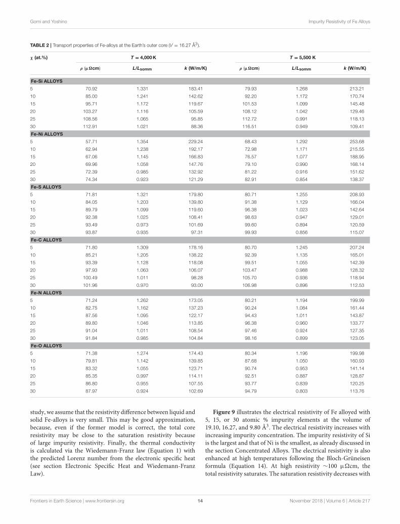
TABLE 2 | Transport properties of Fe-alloys at the Earth’s outer core (V = 16.27 Å3).

χ (at.%) T = 4,000K T = 5,500 K

ρ (µ�cm) L/Lsomm k (W/m/K) ρ (µ�cm) L/Lsomm k (W/m/K)

Fe-Si ALLOYS

5 70.92 1.331 183.41 79.93 1.268 213.21

10 85.00 1.241 142.62 92.20 1.172 170.74

15 95.71 1.172 119.67 101.53 1.099 145.48

20 103.27 1.116 105.59 108.12 1.042 129.46

25 108.56 1.065 95.85 112.72 0.991 118.13

30 112.91 1.021 88.36 116.51 0.949 109.41

Fe-Ni ALLOYS

5 57.71 1.354 229.24 68.43 1.292 253.68

10 62.94 1.238 192.17 72.98 1.171 215.55

15 67.06 1.145 166.83 76.57 1.077 188.95

20 69.96 1.058 147.76 79.10 0.990 168.14

25 72.39 0.985 132.92 81.22 0.916 151.62

30 74.34 0.923 121.29 82.91 0.854 138.37

Fe-S ALLOYS

5 71.81 1.321 179.80 80.71 1.255 208.93

10 84.05 1.203 139.80 91.38 1.129 166.04

15 89.79 1.099 119.60 96.38 1.023 142.64

20 92.38 1.025 108.41 98.63 0.947 129.01

25 93.49 0.973 101.69 99.60 0.894 120.59

30 93.87 0.935 97.31 99.93 0.856 115.07

Fe-C ALLOYS

5 71.80 1.309 178.16 80.70 1.245 207.24

10 85.21 1.205 138.22 92.39 1.135 165.01

15 93.39 1.128 118.08 99.51 1.055 142.39

20 97.93 1.063 106.07 103.47 0.988 128.32

25 100.49 1.011 98.28 105.70 0.936 118.94

30 101.96 0.970 93.00 106.98 0.896 112.53

Fe-N ALLOYS

5 71.24 1.262 173.05 80.21 1.194 199.99

10 82.75 1.162 137.23 90.24 1.084 161.44

15 87.56 1.095 122.17 94.43 1.011 143.87

20 89.80 1.046 113.85 96.38 0.960 133.77

25 91.04 1.011 108.54 97.46 0.924 127.35

30 91.84 0.985 104.84 98.16 0.899 123.05

Fe-O ALLOYS

5 71.38 1.274 174.43 80.34 1.196 199.98

10 79.81 1.142 139.85 87.68 1.050 160.93

15 83.32 1.055 123.71 90.74 0.953 141.14

20 85.35 0.997 114.11 92.51 0.887 128.87

25 86.80 0.955 107.55 93.77 0.839 120.25

30 87.97 0.924 102.69 94.79 0.803 113.76

study, we assume that the resistivity difference between liquid andsolid Fe-alloys is very small. This may be good approximation,because, even if the former model is correct, the total coreresistivity may be close to the saturation resistivity becauseof large impurity resistivity. Finally, the thermal conductivityis calculated via the Wiedemann-Franz law (Equation 1) withthe predicted Lorenz number from the electronic specific heat(see section Electronic Specific Heat and Wiedemann-FranzLaw).

Figure 9 illustrates the electrical resistivity of Fe alloyed with5, 15, or 30 atomic % impurity elements at the volume of19.10, 16.27, and 9.80 Å3. The electrical resistivity increases withincreasing impurity concentration. The impurity resistivity of Siis the largest and that of Ni is the smallest, as already discussed inthe section Concentrated Alloys. The electrical resistivity is alsoenhanced at high temperatures following the Bloch-Grüneisenformula (Equation 14). At high resistivity ∼100 µ�cm, thetotal resistivity saturates. The saturation resistivity decreases with






FIGURE 9 | Electrical resistivity of hcp Fe0.95X0.05, Fe0.85X0.15, and Fe0.70X0.30, where X is Si (purple), Ni (green), S (cyan), C (orange), N (yellow), and O (blue) at thevolume of V = 19.10 Å3 (P∼40 GPa at 300K) (A–C), 16.27 Å3 (P ∼ 120 GPa at 300K) (D–F), and 9.80 Å3 (P ∼ 1,000 GPa at 300K) (G–I). Black broken lines arepure Fe for comparison.

increasing pressure via the Equation (12). Figure 10 representsthe thermal conductivity of Fe alloyed with 5, 15, or 30 atomic% impurity elements at the volume of 19.10, 16.27, and 9.80Å3. The temperature and impurity concentration dependencesof the thermal conductivity are more complicated comparedwith the electrical resistivity. At low temperatures smallerthan ∼5,000K, the thermal conductivities of Fe based alloyshave positive temperature coefficient because of the followingreason. First, it should be noted that the Wiedemann-Franz law(Equation 1) predicts the linear temperature dependence, if theelectrical resistivity and the Lorenz number are independent oftemperature. This condition is nearly satisfied for the electricalresistivity of Fe-light element alloys because, at low temperatures,the impurity resistivity is predominant. Also, as shown inFigure 8, the Lorenz number exhibits positive temperaturecoefficient. Combining these two temperature effects, the thermalconductivity initially increases with increasing temperature.Above 5,000K, the thermal conductivity becomes insensitiveto temperature. The temperature coefficient of the resistivitybecomes small due to the resistivity saturation (Figure 9),whereas the Lorenz number tends to decrease with increasing

temperature (Figure 8). Therefore, the effects of temperatureon the Lorenz number and the linear temperature factor inthe Wiedemann-Franz law are canceled out, which result inthe nearly constant thermal conductivity at high temperature.Table 2 summarized the electrical resistivity, the Lorenz numberand the thermal conductivity of Fe alloys at V = 16.27 Å3 andT = 4,000 or 5,500K, which correspond to the Earth’s outer coreconditions. Considering the compositional effects, our preferredthermal conductivity is higher than∼90 W/m/K.

HEAT FLUX AT THE CMB OFSUPER-EARTHS

The recent developments of astronomical observation can allowto find many terrestrial exoplanets. The exoplanets with themasses of <10 times the Earth’s mass (ME) are so-called super-Earths (e.g., Valencia et al., 2007; Charbonneau et al., 2009).Some of these planets locate within the habitable zone, suggestingthe presence of liquid water at the surface of the planet (e.g.,Anglada-Escudé et al., 2012; Gillon et al., 2017). In term of the






FIGURE 10 | Thermal conductivity of hcp Fe0.95X0.05, Fe0.85X0.15, and Fe0.70X0.30, where X is Si (purple), Ni (green), S (cyan), C (orange), N (yellow), and O (blue) atthe volume of V = 19.10 Å3 (P∼40 GPa at 300K) (A–C), 16.27 Å3 (P∼120 GPa at 300K) (D–F), and 9.80 Å3 (P∼1,000 GPa at 300K) (G–I). Black broken lines arepure Fe for comparison.

surface habitability, the existence of the global magnetic fields isa necessary condition. The planetary magnetic field is generatedvia the geodynamo driven by thermal and/or chemical convectivemotion in the liquid outer core. If super-Earths have thermallydriven geodynamo, the heat flux through the bottom of mantle,qCMB, must be higher than the conductive heat flux along theadiabatic temperature gradient at the top of their core

qs = k

(

∂T

∂r

)

S

= kρdengγ

KST (18)

where k is the thermal conductivity, ρden is the density, g is thegravity, γ is the Grüneisen parameter and KS is the adiabaticbulk modulus. Morard et al. (2011) suggested the absence ofliquid core in the super Earth from the first-principles calculationof melting temperature of Fe. Many studies investigated themantle convection in the super-Earths with varying physicalquantities. The effects of depth increasing mantle viscosity(Tackley et al., 2013), thermal conductivity (Kameyama andYamamoto, 2018) and compressibility (CíŽková et al., 2017)

suppress the mantle convection in the deep portion of the super-Earths. The phase transitions of mantle materials with negativeClapeyron slope also contribute as a stratification of the mantle(Umemoto et al., 2006; Tsuchiya and Tsuchiya, 2011; McWilliamset al., 2012). On the other hand, Stixrude (2014) argued theenergetics of accretion, giant impact and core formation eventsof the super-Earths, and concluded that the mantle convection issufficiently vigorous to sustain the geodynamo. Miyagoshi et al.(2017) demonstrated the occurrence of thermal convection inthe mantle of super-Earth from numerical mantle convectionsimulations with initially hot shallow mantle conditions, which isexpected due to giant impacts. Tachinami et al. (2011) calculatedthe thermal evolution of the cores of super-Earths coupledwith the mixing-length theory for the mantle convective heattransfer, in order to discuss the possibility of the thermallydriven geodynamo. However, they adopted the core thermalconductivity of k = 40 W/m/K, which is one order smaller thanthe present estimate for the 10 Earth mass planet. The purposeof this section is to calculate the conductive heat flux at the topof the liquid core of super-Earths with high thermal conductivityinferred from the previous sections.






To calculate the energy balance in the super-Earths, one-dimensional density and temperature model is required (e.g.,Valencia et al., 2006; Papuc and Davies, 2008; Tachinami et al.,2011). In this study, we read the density profile of super-Earthsfrom Figure 1 of Tachinami et al. (2011). Hence, the planetarymasses of our model are 0.1, 0.2, 0.5, 1, 2, 5, and 10 times to theEarth’s mass (ME). The gravity profile can be calculated from

g(r) = GM(r)

r2(19)

where G = 6.67408 × 10−11 m3/kg/s2 is the gravitationalconstant,M(r) is the inner mass of the radial position r. The massof the inner core Mc is assumed to be 30% of the planetary massMp. The pressure-density relation at the reference temperatureT0 = 300K is given by the Vinet equation of state (EOS):

P(ρden,T0) = 3K0

(

ρden0

ρden

)−2

3

1−

(

ρden0

ρden

)

1

3

exp

3

2

(

K0′ − 1

)

1−

(

ρden0

ρden

)

1

3

(20)

where ρden0 , K0 and K ′

0 are density, bulk modulus and itspressure differentiation at zero pressure, respectively. Theseparameters are given as ρden

0,Fe = 8,300 kg/m3, K0,Fe = 164.8 GPa

and K ′0,Fe = 5.33 for Fe liquid, whereas ρden

0,FeS = 5,330 kg/m3,K0,FeS = 126 GPa and K ′

0,FeS = 4.8 for FeS liquid (see Tachinamiet al., 2011 and references therein). The EOS parameters for theouter core of Fe-FeS liquid mixture are given as function of massfraction of S as

xFeS = xSZFe + ZS

ZS(21)

ρden0,OC =

(

1− xFeS

ρden0,Fe

+xFeS

ρden0,FeS

)−1

(22)

K0,OC =1

ρden0,OC

11− xFeS

ρden0,Fe

1

K0,Fe+

xFeS

ρden0,FeS

1

KFeS

(23)

K′0,OC = −1+ ρden

0,FeK20,OC

(

1− xFeS

ρden0,Fe

1+ K′0,Fe

K20,Fe

+xFeS

ρden0,FeS

1+ K′0,FeS

K20,FeS

)

(24)

where xFe, xFeS are mass fractions of Fe and FeS, ZFe = 55.845and ZS = 32.065 are mass of Fe and S. Following Tachinami et al.(2011), we assumed the bulk S content is set to be x0S = 0.1 andalso assumed that S completely partition into the outer core, themass fraction of S can be calculated as

xS = x0SMc

Mc −Mic(25)

where Mc and Mic are the mass of bulk and inner core,respectively. In this study, we only considered the situation that

Mic = 0.06 Mc, which is close to the present Earth’s value.This leads xS = 0.10638. Our assumption of pure Fe innercore may look unrealistic, however, note that the present heatflux calculation does not refer the chemical composition ofthe inner core. The isothermal bulk modulus at the referencetemperature is obtained by differentiation of the Vinet density-pressure equation of states:

KT

(

ρden,T0

)

=

2K0

1−

(

ρden0

ρden

)

1

3

(

ρden

ρden0

)

2

3(26)

+3

2

(

K′ − 1)

K0

1−

(

ρden0

ρden

)

1

3

(

ρden

ρden0

)

1

3

+ K0

(

ρden

ρden0

)

1

3

exp

3

2

(

K′ − 1)

1−

(

ρden0

ρden

)

1

3

The thermal effect on the equation of states is incorporated asthe thermal corrections by the Mie-Grüneisen equation with theDebye model as:

P(

ρden,T)

= P(

ρden,T0

)

+ 1Pth(ρden,T) (27)

1Pth

(

ρden,T)

=

( γ

V

) (

Eth

(

ρden, T)

− Eth(ρden,T0)

)

(28)

Similarly, the thermal effect on the isothermal bulk modulus isrepresented as follows (Stixrude and Lithgow-Bertelloni, 2005):

KT

(

ρden,T)

= KT

(

ρden,T0

)

+ 1KT(ρden,T) (29)

1KT

(

ρden,T)

=(

γ + 1− q) γ

V

(

Eth

(

ρden,T)

− Eth

(

ρden,T0

))

−γ 2

V

(

TCv

(

ρden,T)

− T0Cv

(

ρden,T0

))

(30)

Eth

(

ρden,T)

= 9nkBT

(

T

2D

)3 ∫ 2DT

0

x3

exp (x) − 1dx (31)

Cv

(

ρden,T)

= 9nkB

(

T

2D

)3 ∫ 2DT

0

x4 exp(x)(

exp (x) − 1)2 dx (32)

where V is the molar volume (1/V = ρden/V0ρden0 ).

KS = KT(1 + 1αγT) (33)

α =γCv

VKT(34)

The Grüneisen parameter can be calculated as follows:

γ = γ0

(

ρden0

ρden

)q

(35)






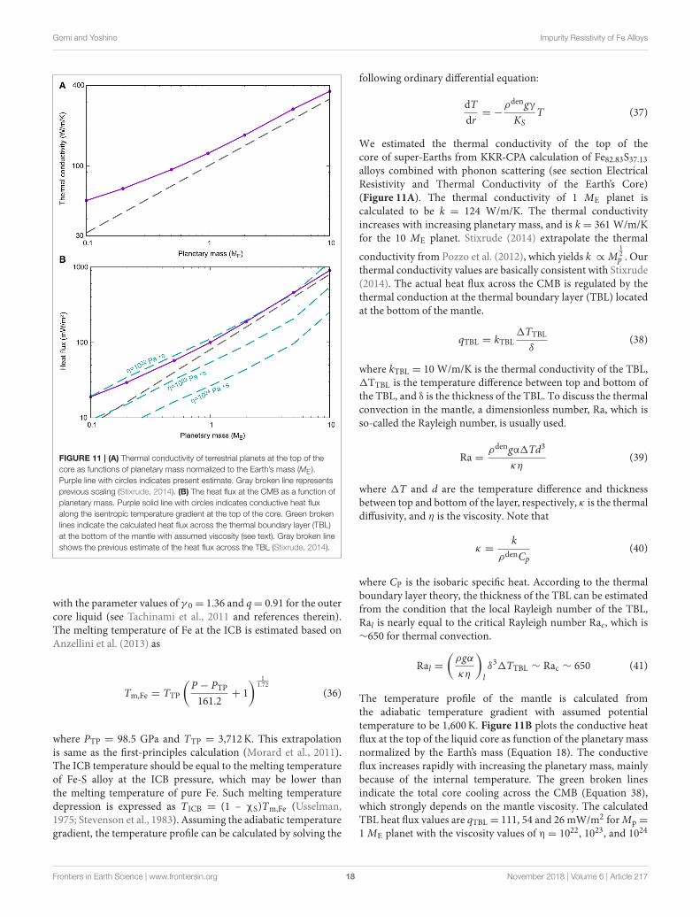
FIGURE 11 | (A) Thermal conductivity of terrestrial planets at the top of thecore as functions of planetary mass normalized to the Earth’s mass (ME).Purple line with circles indicates present estimate. Gray broken line representsprevious scaling (Stixrude, 2014). (B) The heat flux at the CMB as a function ofplanetary mass. Purple solid line with circles indicates conductive heat fluxalong the isentropic temperature gradient at the top of the core. Green brokenlines indicate the calculated heat flux across the thermal boundary layer (TBL)at the bottom of the mantle with assumed viscosity (see text). Gray broken lineshows the previous estimate of the heat flux across the TBL (Stixrude, 2014).

with the parameter values of γ 0 = 1.36 and q= 0.91 for the outercore liquid (see Tachinami et al., 2011 and references therein).The melting temperature of Fe at the ICB is estimated based onAnzellini et al. (2013) as

Tm,Fe = TTP

(

P − PTP

161.2+ 1

)1

1.72

(36)

where PTP = 98.5 GPa and TTP = 3,712K. This extrapolationis same as the first-principles calculation (Morard et al., 2011).The ICB temperature should be equal to the melting temperatureof Fe-S alloy at the ICB pressure, which may be lower thanthe melting temperature of pure Fe. Such melting temperaturedepression is expressed as TICB = (1 – χS)Tm,Fe (Usselman,1975; Stevenson et al., 1983). Assuming the adiabatic temperaturegradient, the temperature profile can be calculated by solving the

following ordinary differential equation:

dT

dr= −

ρdengγ

KST (37)

We estimated the thermal conductivity of the top of thecore of super-Earths from KKR-CPA calculation of Fe82.83S37.13alloys combined with phonon scattering (see section ElectricalResistivity and Thermal Conductivity of the Earth’s Core)(Figure 11A). The thermal conductivity of 1 ME planet iscalculated to be k = 124 W/m/K. The thermal conductivityincreases with increasing planetary mass, and is k = 361 W/m/Kfor the 10 ME planet. Stixrude (2014) extrapolate the thermal

conductivity from Pozzo et al. (2012), which yields k ∝ M12p . Our

thermal conductivity values are basically consistent with Stixrude(2014). The actual heat flux across the CMB is regulated by thethermal conduction at the thermal boundary layer (TBL) locatedat the bottom of the mantle.

qTBL = kTBL1TTBL

δ(38)

where kTBL = 10 W/m/K is the thermal conductivity of the TBL,1TTBL is the temperature difference between top and bottom ofthe TBL, and δ is the thickness of the TBL. To discuss the thermalconvection in the mantle, a dimensionless number, Ra, which isso-called the Rayleigh number, is usually used.

Ra =ρdengα1Td3

κη(39)

where 1T and d are the temperature difference and thicknessbetween top and bottom of the layer, respectively, κ is the thermaldiffusivity, and η is the viscosity. Note that

κ =k

ρdenCp(40)

where CP is the isobaric specific heat. According to the thermalboundary layer theory, the thickness of the TBL can be estimatedfrom the condition that the local Rayleigh number of the TBL,Ral is nearly equal to the critical Rayleigh number Rac, which is∼650 for thermal convection.

Ral =

(

ρgα

κη

)

l

δ31TTBL ∼ Rac ∼ 650 (41)

The temperature profile of the mantle is calculated fromthe adiabatic temperature gradient with assumed potentialtemperature to be 1,600K. Figure 11B plots the conductive heatflux at the top of the liquid core as function of the planetary massnormalized by the Earth’s mass (Equation 18). The conductiveflux increases rapidly with increasing the planetary mass, mainlybecause of the internal temperature. The green broken linesindicate the total core cooling across the CMB (Equation 38),which strongly depends on the mantle viscosity. The calculatedTBL heat flux values are qTBL = 111, 54 and 26 mW/m2 forMp =

1ME planet with the viscosity values of η = 1022, 1023, and 1024






Pa·s, respectively. These values correspond to the Earth’s CMBheat flux, which is ranging from 33 to 99 mW/m2 (5–15 TW)(e.g., Lay et al., 2008). At 1 ME, the core conductive heat flux iscomparable or larger than the thermal boundary layer heat flux.In this case, the liquid core may partly stratify (Labrosse et al.,1997; Lister and Buffett, 1998; Pozzo et al., 2012; Gomi et al.,2013; Labrosse, 2015; Nakagawa, 2017), which is consistent withseismic observation (Tanaka, 2007; Helffrich and Kaneshima,2010). Considering increase of core thermal conductivity withdepth, before the onset of the inner core growth, the fluid coretends to be stratified from the bottom (Gomi et al., 2013).This in turn means that purely thermal buoyancy cannot drivethe convection, if the top of the core is subisentropic. Hence,additional chemical buoyancies are necessary to maintain thegeodynamo. In our Earth, the chemical buoyancy arising fromthe growing inner core contributes large portion of geodynamoefficiency (e.g., Lister and Buffett, 1995; Labrosse, 2015). Recently,MgO or SiO2 precipitation is proposed for another source ofchemical buoyancy (O’rourke and Stevenson, 2016; Hirose et al.,2017). Assuming that the mantle viscosity is independent ofthe planetary mass, the magnitude relation between the coreadiabatic heat flux and the TBL heat flux ofMp > 1ME is similarto that ofMp = 1ME, which suggests that the similar situation ispredicted in the super-Earths: thermally stratified layer at the topof the liquid core and a requirement of chemical buoyancies forgeodynamo.

In this study, we considered only one specific scenariowith many assumptions, however, many scenarios should beconsidered because of large uncertainties of material propertiesother than the thermal conductivity of the core. One ofthe most important uncertainty may be caused by viscosityof the mantle (Tachinami et al., 2011; Tackley et al., 2013).Experimental and theoretical studies suggested that the latticethermal conductivity of the mantle strongly depends on pressure,temperature and phase transitions (Manthilake et al., 2011; Ohtaet al., 2012; Dekura et al., 2013). In addition to the latticethermal conductivity, the radiative conductivity may becomeimportant because it is expected to enhance with temperature,although the value is controversial (Goncharov et al., 2008;Keppler et al., 2008). Since we are interested in the super-Earth located within the habitable zone that have the surfaceliquid water, we assumed that the mantle potential temperaturemay be comparable to that of the Earth T = 1,600K. On theother hand, Stixrude (2014) suggests a higher mantle potentialtemperature due to accretion. Miyagoshi et al. (2017) concludedthat if shallow part of the mantle was hotter than the adiabatictemperature extrapolated from the deeper mantle at the initialstage of mantle convection, such layered structure continuesmore than several billion years. Furthermore, if the temperatureis sufficiently high to melt the mantle material, dynamo processin the magma ocean can also be possible due to high electricalconductivity of melt (McWilliams et al., 2012; Soubiran andMilitzer, 2018). Similarly, the core temperature is also uncertain.We just assumed the inner core radius to determine the coreadiabat, however, Morard et al. (2011) suggested that the coretemperature is too low to melt the metallic core. The internaltemperature should vary with time. Therefore, simulations of

coevolution of thermally coupled mantle and core are needed forthe future work.

SUMMARY

We conducted KKR-CPA-DFT calculations of impurityresistivity of Fe-based light elements (C, N, O, Si, S) or Ni alloys,which is consistent with recent diamond-anvil cell experiments(Gomi and Hirose, 2015; Gomi et al., 2016; Suehiro et al.,2017; Zhang et al., 2018). The results suggest that impurityresistivity of Si is the largest among the light elements candidates,followed by C, S, N, and O (Figure 3). This may be due to thevariation of the saturation resistivity on composition (Figure 5).The impurity resistivity of Ni is smaller than that of five lightelements candidates. The resistivity calculation on Fe-Si-Sternary alloys suggests the violation of the Matthiessen’s rule(Figure 6). We also computed the electronic specific heat of Fealloys, which show the violation of the Sommerfeld expansion(Boness et al., 1986) with low impurity concentration. However,the degree of deviation becomes smaller with increasing impurityconcentration (Figures 7, 8), which suggests that the Sommerfeldvalue of the Lorenz number may be good approximation at theterrestrial cores. The implausibility of geodynamo motion inthe super-Earths has been discussed in terms of the absence ofmantle convection (Tachinami et al., 2011; CíŽková et al., 2017;Kameyama and Yamamoto, 2018). The present study, on theother hand, focused on the thermal conductivity of the core. Wemodeled the thermal conductivity to be higher than∼90W/m/Kfor the Earth’s outer core (Table 2). For the super-Earth with 10ME, the thermal conductivity of the top of the core is estimatedto be 361 W/m/K (Figure 11A), which is one order higher thanthe value of k = 40 W/m/K, which adopted previous thermalevolution calculation (Tachinami et al., 2011) and is consistentwith result from recent scaling calculation (Stixrude, 2014). Theresultant conductive heat flux at the top of the liquid core ofterrestrial planets as function of planetary mass is comparedwith the heat flux across the thermal boundary layer (TBL) at thebottom of mantle (Figure 11B). The present result suggests theabsence of the thermal convection in the core, which predictsthe presence of the thermally stratified layer at the top of thecore of super-Earths, similar to the Earth. In order to sustainthe geodynamo motion in the liquid core, chemical convectionis required, which associates with the inner core growth orprecipitation of MgO and/or SiO2 (O’rourke and Stevenson,2016; Hirose et al., 2017).

AUTHOR CONTRIBUTIONS

HG conducted the calculations. HG and TY wrote themanuscript.

FUNDING

This work was supported by JSPS MEXT/KAKENHI GrantNumber JP15H05827.






ACKNOWLEDGMENTS

We would like to thank Hisazumi Akai for providing theconductivity calculation code implemented in the AkaiKKR

package. The authors also thank to Sonju Kou for fruitfuldiscussion. This work was supported by JSPS MEXT/KAKENHIGrant Number JP15H05827.We are grateful to the two reviewersfor their comments.

REFERENCES

Akai, H. (1989). Fast Korringa-Kohn-Rostoker coherent potentialapproximation and its application to FCC Ni-Fe systems. J Phys. 1, 8045.doi: 10.1088/0953-8984/1/43/006

Alstad, J., Colvin, R., and Legvold, S. (1961). Single-crystal andpolycrystal resistivity relationships for yttrium. Phys. Rev. 123, 418–419.doi: 10.1103/PhysRev.123.418

Anderson, O. L. (1998). The Grüneisen parameter for iron at outer core conditionsand the resulting conductive heat and power in the core. Phys. Earth Planet.

Inter. 109, 179–197. doi: 10.1016/S0031-9201(98)00123-XAnglada-Escudé, G., Arriagada, P., Vogt, S. S., Rivera, E. J., Butler, R. P., Crane,

J. D., et al. (2012). A planetary system around the nearby M dwarf GJ 667Cwith at least one super-Earth in its habitable zone. Astrophys. J. Lett. 751, L16.doi: 10.1088/2041-8205/751/1/L16

Antonov, V. E., Baier, M., Dorner, B., Fedotov, V. K., Grosse, G., Kolesnikov, A.I., et al. (2002). High-pressure hydrides of iron and its alloys. J. Phys. 14, 6427.doi: 10.1088/0953-8984/14/25/311

Anzellini, S., Dewaele, A., Mezouar, M., Loubeyre, P., and Morard, G. (2013).Melting of iron at Earth’s inner core boundary based on fast X-ray diffraction.Science 340, 464–466. doi: 10.1126/science.1233514

Banhart, J., Weinberger, P., and Voitlander, J. (1989). Fermi surface andelectrical resistivity of Cu-Pt alloys: a relativistic calculation. J. Phys. 1, 7013.doi: 10.1088/0953-8984/1/39/012

Bi, Y., Tan, H., and Jing, F. (2002). Electrical conductivity of ironunder shock compression up to 200 GPa. J. Phys. 14, 10849.doi: 10.1088/0953-8984/14/44/389

Bohnenkamp, U., Sandström, R., and Grimvall, G. (2002). Electrical resistivityof steels and face-centered-cubic iron. J. Appl. Phys. 92, 4402–4407.doi: 10.1063/1.1502182

Boness, D. A., and Brown, J. M. (1990). The electronic band structures of iron,sulfur, and oxygen at high pressures and the Earth’s core. J. Geophys. Res. 95,21721–21730. doi: 10.1029/JB095iB13p21721

Boness, D. A., Brown, J. M., and McMahan, A. K. (1986). The electronicthermodynamics of iron under Earth core conditions. Phys. Earth Planet. Inter.42, 227–240. doi: 10.1016/0031-9201(86)90025-7

Butler, W. H. (1985). Theory of electronic transport in random alloys: Korringa-Kohn-Rostoker coherent-potential approximation. Phys. Rev. B 31:3260.doi: 10.1103/PhysRevB.31.3260

Butler, W. H., and Stocks, G. M. (1984). Calculated electrical conductivityand thermopower of silver-palladium alloys. Phys. Rev. B 29, 4217.doi: 10.1103/PhysRevB.29.4217

Charbonneau, D., Berta, Z. K., Irwin, J., Burke, C. J., Nutzman, P., Buchhave, L. A.,et al. (2009). A super-Earth transiting a nearby low-mass star. Nature 462, 891.doi: 10.1038/nature08679

CíŽková, H., van den Berg, A., and Jacobs, M. (2017). Impact of compressibilityon heat transport characteristics of large terrestrial planets. Phys. Earth Planet.

Inter. 268, 65–77. doi: 10.1016/j.pepi.2017.04.007Cote, P. J., and Meisel, L. V. (1978). Origin of saturation effects in electron

transport. Phys. Rev. Lett. 40, 1586–1589. doi: 10.1103/PhysRevLett.40.1586Cusack, N., and Enderby, J. E. (1960). A note on the resistivity of liquid

alkali and noble metals. Proc. Phys. Soc. 75, 395. doi: 10.1088/0370-1328/75/3/310

de Koker, N., Steinle-Neumann, G., and Vlcek, V. (2012). Electrical resistivityand thermal conductivity of liquid Fe alloys at high P and T, andheat flux in Earth’s core. Proc. Natl. Acad. Sci. U.S.A. 109, 4070–4073.doi: 10.1073/pnas.1111841109

Dekura, H., Tsuchiya, T., and Tsuchiya, J. (2013). Ab initio lattice thermalconductivity of MgSiO3 perovskite as found in Earth’s lower mantle. Phys. Rev.Lett. 110:025904. doi: 10.1103/PhysRevLett.110.025904

Deng, L., Seagle, C., Fei, Y., and Shahar, A. (2013). High pressure and temperatureelectrical resistivity of iron and implications for planetary cores. Geophys. Res.Lett. 40, 33–37. doi: 10.1029/2012GL054347

Dewaele, A., Loubeyre, P., Occelli, F., Mezouar, M., Dorogokupets, P. I., andTorrent, M. (2006). Quasihydrostatic equation of state of iron above 2 Mbar.Phys. Rev. Lett. 97:215504. doi: 10.1103/PhysRevLett.97.215504

Dobson, D. (2016). Geophysics: earth’s core problem. Nature 534, 45.doi: 10.1038/534045a

Drchal, V., Kudrnovský, J., Wagenknecht, D., Turek, I., and Khmelevskyi, S.(2017). Transport properties of iron at Earth’s core conditions: the effect of spindisorder. Phys. Rev. B 96:024432. doi: 10.1103/PhysRevB.96.024432

Ezenwa, I. C., and Secco, R. A. (2017a). Constant electrical resistivity of Znalong the melting boundary up to 5 GPa. High Press. Res. 37, 319–333.doi: 10.1080/08957959.2017.1340473

Ezenwa, I. C., and Secco, R. A. (2017b). Electronic transition in solid Nb at highpressure and temperature. J. Appl. Phys. 121, 225903. doi: 10.1063/1.4985548

Ezenwa, I. C., and Secco, R. A. (2017c). Invariant electrical resistivity ofCo along the melting boundary. Earth Planet. Sci. Lett. 474, 120–127.doi: 10.1016/j.epsl.2017.06.032

Ezenwa, I. C., Secco, R. A., Yong, W., Pozzo, M., and Alfè, D. (2017). Electricalresistivity of solid and liquid Cu up to 5 GPa: decrease along the meltingboundary. J. Phys. Chem. Solids 110, 386–393. doi: 10.1016/j.jpcs.2017.06.030

Faber, T. E. (1972). An Introduction to the Theory of Liquid Metals. Cambridge:Cambridge University Press.

Friedel, J. (1956). On some electrical and magnetic properties of metallic solidsolutions. Can. J. Phys. 34, 1190–1211. doi: 10.1139/p56-134

Fukai, Y. (2006).TheMetal-Hydrogen System: Basic Bulk Properties, Vol. 21. Berlin;Heidelberg; New York, NY: Springer Science & Business Media.

Gillon, M., Triaud, A. H., Demory, B. O., Jehin, E., Agol, E., Deck, K. M., et al.(2017). Seven temperate terrestrial planets around the nearby ultracool dwarfstar TRAPPIST-1. Nature 542, 456. doi: 10.1038/nature21360

Glasbrenner, J. K., Pujari, B. S., and Belashchenko, K. D. (2014). Deviations fromMatthiessen’s rule and resistivity saturation effects in Gd and Fe from firstprinciples. Phys. Rev. B 89:174408. doi: 10.1103/PhysRevB.89.174408

Gomi, H., Fei, Y., and Yoshino, T. (2018). The effects of ferromagnetismand interstitial hydrogen on the equation of states of hcp and dhcp FeHx :implications for the Earth’s inner core age. Am. Mineral. 103, 1271–1281.doi: 10.2138/am-2018-6295

Gomi, H., and Hirose, K. (2015). Electrical resistivity and thermal conductivityof hcp Fe–Ni alloys under high pressure: implications for thermalconvection in the Earth’s core. Phys. Earth Planet. Inter. 247, 2–10.doi: 10.1016/j.pepi.2015.04.003

Gomi, H., Hirose, K., Akai, H., and Fei, Y. (2016). Electrical resistivity ofsubstitutionally disordered hcp Fe–Si and Fe–Ni alloys: chemically-inducedresistivity saturation in the Earth’s core. Eart Planet. Sci. Lett. 451, 51–61.doi: 10.1016/j.epsl.2016.07.011

Gomi, H., Ohta, K., Hirose, K., Labrosse, S., Caracas, R., Verstraete, M. J., et al.(2013). The high conductivity of iron and thermal evolution of the Earth’s core.Phys. Earth Planet. Inter. 224, 88–103. doi: 10.1016/j.pepi.2013.07.010

Goncharov, A. F., Haugen, B. D., Struzhkin, V. V., Beck, P., and Jacobsen, S. D.(2008). Radiative conductivity in the Earth’s lower mantle. Nature 456, 231.doi: 10.1038/nature07412

Gurvitch, M. (1981). Ioffe-Regel criterion and resistivity of metals. Phys. Rev. B24:7404. doi: 10.1103/PhysRevB.24.7404

Helffrich, G., and Kaneshima, S. (2010). Outer-core compositionalstratification from observed core wave speed profiles. Nature 468, 807.doi: 10.1038/nature09636

Hieu, H. K., Hai, T. T., Hong, N. T., Sang, N. D., and Tuyen, N. V. (2017). Electricalresistivity and thermodynamic properties of iron under high pressure. J. Electr.Mater. 46, 3702–3706. doi: 10.1007/s11664-017-5411-2


https://doi.org/10.1088/0953-8984/1/43/006

https://doi.org/10.1103/PhysRev.123.418

https://doi.org/10.1016/S0031-9201(98)00123-X

https://doi.org/10.1088/2041-8205/751/1/L16

https://doi.org/10.1088/0953-8984/14/25/311

https://doi.org/10.1126/science.1233514

https://doi.org/10.1088/0953-8984/1/39/012

https://doi.org/10.1088/0953-8984/14/44/389

https://doi.org/10.1063/1.1502182

https://doi.org/10.1029/JB095iB13p21721

https://doi.org/10.1016/0031-9201(86)90025-7

https://doi.org/10.1103/PhysRevB.31.3260


https://doi.org/10.1038/nature08679

https://doi.org/10.1016/j.pepi.2017.04.007

https://doi.org/10.1103/PhysRevLett.40.1586

https://doi.org/10.1088/0370-1328/75/3/310

https://doi.org/10.1073/pnas.1111841109


https://doi.org/10.1029/2012GL054347


https://doi.org/10.1038/534045a


https://doi.org/10.1080/08957959.2017.1340473

https://doi.org/10.1063/1.4985548

https://doi.org/10.1016/j.epsl.2017.06.032

https://doi.org/10.1016/j.jpcs.2017.06.030

https://doi.org/10.1139/p56-134



https://doi.org/10.2138/am-2018-6295







https://doi.org/10.1007/s11664-017-5411-2





Hirose, K., Labrosse, S., and Hernlund, J. (2013). Composition andstate of the core. Annu. Rev. Earth Planet. Sci. 41, 657–691.doi: 10.1146/annurev-earth-050212-124007

Hirose, K., Morard, G., Sinmyo, R., Umemoto, K., Hernlund, J., Helffrich, G., et al.(2017). Crystallization of silicon dioxide and compositional evolution of theEarth’s core. Nature 543, 99. doi: 10.1038/nature21367

Kameyama, M., and Yamamoto, M. (2018). Numerical experiments on thermalconvection of highly compressible fluids with variable viscosity and thermalconductivity: implications for mantle convection of super-Earths. Phys. EarthPlanet. Inter. 274, 23–36. doi: 10.1016/j.pepi.2017.11.001

Keppler, H., Dubrovinsky, L. S., Narygina, O., and Kantor, I. (2008). Opticalabsorption and radiative thermal conductivity of silicate perovskite to 125gigapascals. Science 322, 1529–1532. doi: 10.1126/science.1164609

Kiarasi, S., and Secco, R. A. (2015). Pressure-induced electrical resistivitysaturation of Fe17Si. Phys. Status Solidi (b) 252, 2034–2042.doi: 10.1002/pssb.201552029

Konôpková, Z., Lazor, P., Goncharov, A. F., and Struzhkin, V. V. (2011). Thermalconductivity of hcp iron at high pressure and temperature. High Press. Res. 31,228–236. doi: 10.1080/08957959.2010.545059

Konôpková, Z., McWilliams, R. S., Gómez-Pérez, N., and Goncharov, A. F. (2016).Direct measurement of thermal conductivity in solid iron at planetary coreconditions. Nature 534, 99. doi: 10.1038/nature18009

Kou, S., and Akai, H. (2018). First-principles calculation of transition-metalSeebeck coefficients. Solid State Commun. 276, 1–4. doi: 10.1016/j.ssc.2018.02.018

Kuwayama, Y., Hirose, K., Sata, N., and Ohishi, Y. (2008). Phase relations ofiron and iron-nickel alloys up to 300 GPa: implications for compositionand structure of the Earth’s inner core. Earth Planet. Sci. Lett. 273, 379–385.doi: 10.1016/j.epsl.2008.07.001

Labrosse, S. (2015). Thermal evolution of the core with a high thermalconductivity. Phys. Earth Planet. Inter. 247, 36–55. doi: 10.1016/j.pepi.2015.02.002

Labrosse, S., Poirier, J. P., and LeMouël, J. L. (1997). On cooling of the Earth’s core.Phys. Earth Planet. Inter. 99, 1–17. doi: 10.1016/S0031-9201(96)03207-4

Lay, T., Hernlund, J., and Buffett, B. A. (2008). Core–mantle boundary heat flow.Nat. Geosci. 1, 25. doi: 10.1038/ngeo.2007.44

Lin, Z., Zhigilei, L. V., and Celli, V. (2008). Electron-phonon coupling andelectron heat capacity of metals under conditions of strong electron-phonon nonequilibrium. Phys. Rev. B 77:075133. doi: 10.1103/PhysRevB.77.075133

Linde, J. O. (1932). Elektrische Eigenschaften verdünnter MischkristallegierungenIII. Widerstand von Kupfer-und Goldlegierungen. Gesetzmäßigkeitender Widerstandserhöhungen. Ann. Phys. 407, 219–248.doi: 10.1002/andp.19324070206

Lister, J. R., and Buffett, B. A. (1995). The strength and efficiency of thermal andcompositional convection in the geodynamo. Phys. Earth Planet. Inter. 91,17–30. doi: 10.1016/0031-9201(95)03042-U

Lister, J. R., and Buffett, B. A. (1998). Stratification of the outer coreat the core-mantle boundary. Phys. Earth Planet. Inter. 105, 5–19.doi: 10.1016/S0031-9201(97)00082-4

Manthilake, G. M., de Koker, N., Frost, D. J., andMcCammon, C. A. (2011). Latticethermal conductivity of lower mantle minerals and heat flux from Earth’s core.Proc. Natl. Acad. Sci. U.S.A. 108, 17901–17904. doi: 10.1073/pnas.1110594108

Markowitz, D. (1977). Calculation of electrical resistivity of highly resistivemetallicalloys. Phys. Rev. B 15:3617. doi: 10.1103/PhysRevB.15.3617

Matassov, G. (1977). The Electrical Conductivity of Iron-Silicon Alloys at High

Pressures and the Earth’s Core. Ph.D. thesis, Lawrence Livermore Laboratory,University of California.

McWilliams, R. S., Konôpková, Z., and Goncharov, A. F. (2015). A flashheating method for measuring thermal conductivity at high pressure andtemperature: application to Pt. Phys. Earth Planet. Inter. 247, 17–26.doi: 10.1016/j.pepi.2015.06.002

McWilliams, R. S., Spaulding, D. K., Eggert, J. H., Celliers, P. M., Hicks, D.G., Smith, R. F., et al. (2012). Phase transformations and metallization ofmagnesium oxide at high pressure and temperature. Science 338, 1330–1333.doi: 10.1126/science.1229450

Mertig, I. (1999). Transport properties of dilute alloys. Rep. Prog. Phys. 62, 237.doi: 10.1088/0034-4885/62/2/004

Miyagoshi, T., Kameyama, M., and Ogawa, M. (2017). Extremely long transitionphase of thermal convection in the mantle of massive super-Earths. EarthPlanets Space 69, 46. doi: 10.1186/s40623-017-0630-6

Mooij, J. H. (1973). Electrical conduction in concentrated disordered transitionmetal alloys. Phys. Status Solidi 17, 521–530. doi: 10.1002/pssa.2210170217

Morard, G., Bouchet, J., Valencia, D., Mazevet, S., and Guyot, F. (2011). Themelting curve of iron at extreme pressures: implications for planetary cores.High Energy Density Phys. 7, 141–144. doi: 10.1016/j.hedp.2011.02.001

Moruzzi, V. L., Janak, J. F., and Williams, A. R. (1978). Calculated Electronic

Properties of Metals. New York, NY: Pergamon Press Inc.Mott, N. F. (1934). The resistance of liquid metals. Proc. R. Soc. Lond. A 146,

465–472. doi: 10.1098/rspa.1934.0166Mott, N. F. (1936). “The electrical resistance of dilute solid solutions,” in

Mathematical Proceedings of the Cambridge Philosophical Society, Vol. 32(Cambridge: Cambridge University Press), 281–290.

Mott, N. F. (1972). The electrical resistivity of liquid transition metals. Philos. Mag.

26, 1249–1261. doi: 10.1080/14786437208220339Nakagawa, T. (2017). On the thermo-chemical origin of the stratified region

at the top of the Earth’s core. Phys. Earth Planet. Inter. 276, 172–181.doi: 10.1016/j.pepi.2017.05.011

Norbury, A. L. (1921). The electrical resistivity of dilute metallic solid solutions.Trans. Faraday Soc. 16, 570–596. doi: 10.1039/tf9211600570

Ohta, K., Kuwayama, Y., Hirose, K., Shimizu, K., and Ohishi, Y. (2016).Experimental determination of the electrical resistivity of iron at Earth’s coreconditions. Nature 534, 95. doi: 10.1038/nature17957

Ohta, K., Suehiro, S., Hirose, K., and Ohishi, Y. (2018). Electrical resistivity of fccphase iron hydrides at high pressure and temperatures. Comptes Rendus Geosci.doi: 10.1016/j.crte.2018.05.004. [Epub ahead of print].

Ohta, K., Yagi, T., Taketoshi, N., Hirose, K., Komabayashi, T., Baba, T.,et al. (2012). Lattice thermal conductivity of MgSiO3 perovskite and post-perovskite at the core–mantle boundary. Earth Planet. Sci. Lett. 349, 109–115.doi: 10.1016/j.epsl.2012.06.043

O’rourke, J. G., and Stevenson, D. J. (2016). Powering Earth’s dynamowith magnesium precipitation from the core. Nature 529, 387.doi: 10.1038/nature16495

Oshita, M., Yotsuhashi, S., Adachi, H., and Akai, H. (2009). Seebeck coefficientcalculated by kubo–greenwood formula on the basis of density functionaltheory. J. Phys. Soc. Jpn. 78:024708. doi: 10.1143/JPSJ.78.024708

Ozawa, H., Hirose, K., Yonemitsu, K., and Ohishi, Y. (2016). High-pressure melting experiments on Fe-Si alloys and implications forsilicon as a light element in the core. Earth Planet. Sci. Lett. 456, 47–54.doi: 10.1016/j.epsl.2016.08.042

Papuc, A. M., and Davies, G. F. (2008). The internal activity and thermal evolutionof Earth-like planets. Icarus 195, 447–458. doi: 10.1016/j.icarus.2007.12.016

Poirier, J. P. (2000). Introduction to the Physics of the Earth’s Interior. Cambridge:Cambridge University Press.

Pommier, A. (2018). Influence of sulfur on the electrical resistivity of acrystallizing core in small terrestrial bodies. Earth Planet. Sci. Lett. 496, 37–46.doi: 10.1016/j.epsl.2018.05.032

Pourovskii, L. V., Mravlje, J., Georges, A., Simak, S. I., and Abrikosov, I. A. (2017).Electron–electron scattering and thermal conductivity of ǫfnduc at Earth’s coreconditions. New J. Phys. 19, 073022. doi: 10.1088/1367-2630/aa76c9

Pozzo, M., and Alfè, D. (2016a). Saturation of electrical resistivity of solid iron atEarth’s core conditions. Springerplus 5, 256. doi: 10.1186/s40064-016-1829-x

Pozzo, M., and Alfè, D. (2016b). “Electrical resistivity saturation of solid ironat Earth’s core conditions from density functional theory,” in AGU Abstract

DI13A-2356, AGU Fall Meeting (San Fransisco, CA).Pozzo, M., Davies, C., Gubbins, D., and Alfè, D. (2012). Thermal and

electrical conductivity of iron at Earth’s core conditions. Nature 485, 355.doi: 10.1038/nature11031

Pozzo, M., Davies, C., Gubbins, D., and Alfè, D. (2013). Transport properties forliquid silicon-oxygen-iron mixtures at Earth’s core conditions. Phys. Rev. B87:014110. doi: 10.1103/PhysRevB.87.014110

Pozzo, M., Davies, C., Gubbins, D., and Alfè, D. (2014). Thermal and electricalconductivity of solid iron and iron–silicon mixtures at Earth’s core conditions.Earth Planet. Sci. Lett. 393, 159–164. doi: 10.1016/j.epsl.2014.02.047

Seagle, C. T., Cottrell, E., Fei, Y., Hummer, D. R., and Prakapenka, V. B. (2013).Electrical and thermal transport properties of iron and iron-silicon alloy


https://doi.org/10.1146/annurev-earth-050212-124007




https://doi.org/10.1002/pssb.201552029

https://doi.org/10.1080/08957959.2010.545059


https://doi.org/10.1016/j.ssc.2018.02.018



https://doi.org/10.1016/S0031-9201(96)03207-4

https://doi.org/10.1038/ngeo.2007.44


https://doi.org/10.1002/andp.19324070206

https://doi.org/10.1016/0031-9201(95)03042-U

https://doi.org/10.1016/S0031-9201(97)00082-4





https://doi.org/10.1088/0034-4885/62/2/004

https://doi.org/10.1186/s40623-017-0630-6

https://doi.org/10.1002/pssa.2210170217

https://doi.org/10.1016/j.hedp.2011.02.001

https://doi.org/10.1098/rspa.1934.0166

https://doi.org/10.1080/14786437208220339


https://doi.org/10.1039/tf9211600570


https://doi.org/10.1016/j.crte.2018.05.004



https://doi.org/10.1143/JPSJ.78.024708


https://doi.org/10.1016/j.icarus.2007.12.016


https://doi.org/10.1088/1367-2630/aa76c9

https://doi.org/10.1186/s40064-016-1829-x








at high pressure. Geophys. Res. Lett. 40, 5377–5381. doi: 10.1002/2013GL057930

Secco, R. A. (2017). Thermal conductivity and Seebeck coefficientof Fe and Fe-Si alloys: implications for variable Lorenz number.Phys. Earth Planet. Inter. 265, 23–34. doi: 10.1016/j.pepi.2017.01.005

Secco, R. A., and Schloessin, H. H. (1989). The electrical resistivity of solidand liquid Fe at pressures up to 7 GPa. J. Geophys. Res. 94, 5887–5894.doi: 10.1029/JB094iB05p05887

Sha, X., and Cohen, R. E. (2011). First-principles studies of electrical resistivity ofiron under pressure. J. Phys. 23:075401. doi: 10.1088/0953-8984/23/7/075401

Silber, R. E., Secco, R. A., and Yong, W. (2017). Constant electrical resistivity ofNi along the melting boundary up to 9 GPa. J. Geophys. Res.122, 5064–5081.doi: 10.1002/2017JB014259

Silber, R. E., Secco, R. A., Yong, W., and Littleton, J. A. (2018). Electrical resistivityof liquid Fe to 12 GPa: implications for heat flow in cores of terrestrial bodies.Sci. Rep. 8, 10758. doi: 10.1038/s41598-018-28921-w

Smith, R. F., Fratanduono, D. E., Braun, D. G., Duffy, T. S., Wicks, J. K., Celliers, P.M., et al. (2018). Equation of state of iron under core conditions of large rockyexoplanets. Nat. Astron. 2, 452–458. doi: 10.1038/s41550-018-0437-9

Soubiran, F., and Militzer, B. (2018). Electrical conductivity and magneticdynamos in magma oceans of Super-Earths. Nat. Commun. 9, 3883.doi: 10.1038/s41467-018-06432-6

Stacey, F. D., and Anderson, O. L. (2001). Electrical and thermal conductivities ofFe–Ni–Si alloy under core conditions. Phys. Earth Planet. Inter. 124, 153–162.doi: 10.1016/S0031-9201(01)00186-8

Stacey, F. D., and Loper, D. E. (2007). A revised estimate of the conductivity of ironalloy at high pressure and implications for the core energy balance. Phys. EarthPlanet. Inter. 161, 13–18. doi: 10.1016/j.pepi.2006.12.001

Stevenson, D. J., Spohn, T., and Schubert, G. (1983). Magnetism andthermal evolution of the terrestrial planets. Icarus 54, 466–489.doi: 10.1016/0019-1035(83)90241-5

Stixrude, L. (2012). Structure of Iron to 1 Gbar and 40 000K. Phys. Rev. Lett.108:055505. doi: 10.1103/PhysRevLett.108.055505

Stixrude, L. (2014). Melting in super-earths. Philos. Trans. R. Soc. Lond. A Math.

Phys. Eng. Sci. 372, 20130076. doi: 10.1098/rsta.2013.0076Stixrude, L., and Lithgow-Bertelloni, C. (2005). Thermodynamics of

mantle minerals—I. Physical properties. Geophys. J. Int. 162, 610–632.doi: 10.1111/j.1365-246X.2005.02642.x

Suehiro, S., Ohta, K., Hirose, K., Morard, G., and Ohishi, Y. (2017). Theinfluence of sulfur on the electrical resistivity of hcp iron: implications forthe core conductivity of Mars and Earth. Geophys. Res. Lett. 44, 8254–8259.doi: 10.1002/2017GL074021

Tachinami, C., Senshu, H., and Ida, S. (2011). Thermal evolution and lifetime ofintrinsic magnetic fields of super-Earths in habitable zones.Astrophys. J. 726:70.doi: 10.1088/0004-637X/726/2/70

Tackley, P. J., Ammann, M., Brodholt, J. P., Dobson, D. P., and Valencia, D. (2013).Mantle dynamics in super-Earths: post-perovskite rheology and self-regulationof viscosity. Icarus 225, 50–61. doi: 10.1016/j.icarus.2013.03.013

Tanaka, S. (2007). Possibility of a low P-wave velocity layer in the outermostcore from global SmKS waveforms. Earth Planet. Sci. Lett. 259, 486–499.doi: 10.1016/j.epsl.2007.05.007

Tateno, S., Hirose, K., Ohishi, Y., and Tatsumi, Y. (2010). The structure of iron inEarth’s inner core. Science 330, 359–361. doi: 10.1126/science.1194662

Tateno, S., Kuwayama, Y., Hirose, K., and Ohishi, Y. (2015). The structureof Fe-Si alloy in Earth’s inner core. Earth Planet. Sci. Lett. 418, 11–19.doi: 10.1016/j.epsl.2015.02.008

Tsiovkin, Y. Y., Voloshinskii, A. N., Gapontsev, V. V., and Ustinov, V. V. (2005).Residual electrical resistivity in dilute nonmagnetic alloys of transition metals.Phys. Rev. B 71:184206. doi: 10.1103/PhysRevB.71.184206

Tsiovkin, Y. Y., Voloshinskii, A. N., Gapontsev, V. V., and Ustinov, V. V. (2006).Theory of the residual resistivity of dilute alloys of nonmagnetic 3 d−5 dtransition metals. Low Temp. Phys. 32, 863–867. doi: 10.1063/1.2356843

Tsuchiya, T., and Kawamura, K. (2002). First-principles electronicthermal pressure of metal Au and Pt. Phys. Rev. B 66:094115.doi: 10.1103/PhysRevB.66.094115

Tsuchiya, T., and Tsuchiya, J. (2011). Prediction of a hexagonal SiO2 phase affectingstabilities of MgSiO3 and CaSiO3 at multimegabar pressures. Proc. Natl. Acad.Sci. U.S.A. 108, 1252–1255. doi: 10.1073/pnas.1013594108

Tsumuraya, T., Matsuura, Y., Shishidou, T., and Oguchi, T. (2012). First-principlesstudy on the structural and magnetic properties of iron hydride. J. Phys. Soc.Jpn. 81:064707. doi: 10.1143/JPSJ.81.064707

Umemoto, K., Wentzcovitch, R. M., and Allen, P. B. (2006). Dissociation ofMgSiO3 in the cores of gas giants and terrestrial exoplanets. Science 311,983–986. doi: 10.1126/science.1120865

Usselman, T. M. (1975). Experimental approach to the state of the core; Part I,The liquidus relations of the Fe-rich portion of the Fe-Ni-S system from 30 to100 kb. Am. J. Sci. 275, 278–290. doi: 10.2475/ajs.275.3.278

Vafayi, K., Calandra, M., and Gunnarsson, O. (2006). Electronic thermalconductivity at high temperatures: violation of the Wiedemann-Franz law innarrow-band metals. Phys. Rev. B 74:235116. doi: 10.1103/PhysRevB.74.235116

Valencia, D., O’Connell, R. J., and Saselov, D. (2006). Internal structure of massiveterrestrial planets. Icarus 181, 545–554. doi: 10.1016/j.icarus.2005.11.021

Valencia, D., Sasselov, D. D., and O’Connell, R. J. (2007). Radius andstructure models of the first super-Earth planet. Astrophys. J. 656, 545.doi: 10.1086/509800

Van Zytveld, J. B. (1980). Electrical resistivities of liquid transition metals. Le J.Phys. Colloques 41, C8–C503. doi: 10.1051/jphyscol:19808126

Wagle, F., and Steinle-Neumann, G. (2018). Electrical resistivity discontinuityof iron along the melting curve. Geophys. J. Int. 213, 237–243.doi: 10.1093/gji/ggx526

Wagle, F., Steinle-Neumann, G., and de Koker, N. (2018). Saturation and negativetemperature coefficient of electrical resistivity in liquid iron-sulfur alloysat high densities from first principles calculations. Phys. Rev. B 97:094307.doi: 10.1103/PhysRevB.97.094307

Wicks, J. K., Smith, R. F., Fratanduono, D. E., Coppari, F., Kraus, R. G., Newman,M. G., et al. (2018). Crystal structure and equation of state of Fe-Si alloys atsuper-Earth core conditions. Sci. Adv. 4:eaao5864. doi: 10.1126/sciadv.aao5864

Williams, Q. (2018). The thermal conductivity of Earth’s core: a key geophysicalparameter’s constraints and uncertainties. Annu. Rev. Earth Planet. Sci. 46,47–66. doi: 10.1146/annurev-earth-082517-010154

Xu, J., Zhang, P., Haule, K., Minar, J., Wimmer, S., Ebert, H., et al.(2018). Thermal conductivity and electrical resistivity of solid iron atEarth’s core conditions from first principles. Phys. Rev. Lett. 121:096601.doi: 10.1103/PhysRevLett.121.096601

Yue, S. Y., and Hu, M. (2018). Insight of the thermal conductivity of ε iron atEarth’s core conditions from the newly developed direct ab initiomethodology.arXiv:1808.10860 [Preprint].

Zhang, C., Lin, J. F., Liu, Y., Feng, S., Jin, C., Hou, M., et al. (2018). Electricalresistivity of Fe-C alloy at high pressure: effects of carbon as a light element onthe thermal conductivity of the Earth’s core. J. Geophys. Res. 123, 3564–3577.doi: 10.1029/2017JB015260

Ziman, J. M. (1961). A theory of the electrical properties of liquid metals.I: the monovalent metals. Philos. Mag. 6, 1013–1034. doi: 10.1080/14786436108243361

Conflict of Interest Statement: The authors declare that the research wasconducted in the absence of any commercial or financial relationships that couldbe construed as a potential conflict of interest.

Copyright © 2018 Gomi and Yoshino. This is an open-access article distributed

under the terms of the Creative Commons Attribution License (CC BY). The use,

distribution or reproduction in other forums is permitted, provided the original

author(s) and the copyright owner(s) are credited and that the original publication

in this journal is cited, in accordance with accepted academic practice. No use,

distribution or reproduction is permitted which does not comply with these terms.


https://doi.org/10.1002/2013GL057930


https://doi.org/10.1029/JB094iB05p05887

https://doi.org/10.1088/0953-8984/23/7/075401

https://doi.org/10.1002/2017JB014259

https://doi.org/10.1038/s41598-018-28921-w

https://doi.org/10.1038/s41550-018-0437-9

https://doi.org/10.1038/s41467-018-06432-6

https://doi.org/10.1016/S0031-9201(01)00186-8


https://doi.org/10.1016/0019-1035(83)90241-5


https://doi.org/10.1098/rsta.2013.0076

https://doi.org/10.1111/j.1365-246X.2005.02642.x

https://doi.org/10.1002/2017GL074021

https://doi.org/10.1088/0004-637X/726/2/70






https://doi.org/10.1063/1.2356843



https://doi.org/10.1143/JPSJ.81.064707


https://doi.org/10.2475/ajs.275.3.278



https://doi.org/10.1086/509800

https://doi.org/10.1051/jphyscol:19808126

https://doi.org/10.1093/gji/ggx526


https://doi.org/10.1126/sciadv.aao5864

https://doi.org/10.1146/annurev-earth-082517-010154


https://doi.org/10.1029/2017JB015260

https://doi.org/10.1080/14786436108243361

http://creativecommons.org/licenses/by/4.0/








Impurity Resistivity of fcc and hcp Fe-Based Alloys ...

Documents

Transcript of Impurity Resistivity of fcc and hcp Fe-Based Alloys ...