Impulsive Control of Lagrangian Systems

and Locomotion in Fluids

Alberto Bressan

Department of Mathematics, Penn State University, University Park, Pa. 16802 U.S.A.e-mail: bressan@math.psu.edu

Abstract. Aim of this paper is to provide a survey of the theory of impulsive control of Lagrangiansystems. It is assumed here that an external controller can determine the evolution of the systemby directly prescribing the values of some of the coordinates. We begin by motivating the theorywith a couple of elementary examples. Then we discuss the analytical form taken by the equationsof motion, and their impulsive character. The following sections review various results found inthe literature concerning the continuity of the control-to-trajectory map, the existence of optimalcontrols, and the asymptotic controllability to a reference state. In the last section we indicate afurther application of the theory, to the control of deformable bodies immersed in a fluid.

1 - Introduction

In the control literature, by “impulsive control system” one usually refers to a system governedby a differential equation

d

dtx(t) = f

(t, x(t), u(t)

), (1.1)

but where the state x is also allowed to jump, at a finite set times:

x(ti+) = Φ(ti, x(ti−), αi

).

Here the controller selects the control function u(·), as well as the times ti and the parameters αi

determining the jumps [BL].There is also a quite different framework leading to impulsive control. Namely, consider

a Lagrangian system described by coordinates q = (q1, . . . , qn+m). Assume that, by imposingsuitable mechanical constraints, we can directly assign some of these coordinates as functionsof time, say qi(t) = ui(t) for i = n + 1, . . . , n + m. One can then show that the evolution ofthe remaining free coordinates q1, . . . , qn is determined by a first order system of 2n differentialequations of the form

qi = φi

(t, q(t), p(t), u(t), u(t)

),

pi = ψi

(t, q(t), p(t), u(t), u(t)

),

i = 1, . . . , n , (1.2)

1

where upper dots denote derivatives w.r.t. time. Here p1, . . . , pn are the so-called conjugate mo-ments, i.e. pj = ∂T/∂qj , with T = T (q, q) denoting the kinetic energy of the system. See (3.6) inSection 3 for details.

Notice that the right hand side of (1.2) also contains the time derivative of the control u(·).If this control function is discontinuous, the motion will thus have an impulsive character. It is onthis second type of impulsive systems that we focus our interest, throughout the present paper.

The theory of control of Lagrangian systems by means of of moving constraints was initiatedindependently by Aldo Bressan and by Charles-Michel Marle, around 1980. The memoir [AB1]was motivated by problems of optimal control for the ski or the swing, later studied in [AB2]. In[Ma] one can find a more general geometric approach, also including some mechanical applications.The connections between the two approaches were clarified in [CF].

The mathematical theory for these problems has been concerned with various issues, whichwe briefly review.

1. Form of the equations. The equations (1.2) constitute a system of n+ n equations for thefirst-order time derivatives q1, . . . qn, p1 , . . . , pn. In general, one can show that the right hand sidesof these O.D.E’s are polynomials of degree ≤ 2 w.r.t. the derivatives ui. Renaming the variablesx = (x1, . . . , x2n) = (q1, . . . qn , p1, . . . , pn), this means we have a system of the form

x = f(t, x, u) +m∑

i=1

gi(t, x, u) ui +m∑

i,j=1

hij(t, x, u) uiuj . (1.3)

The explicit dependence of the vector fields f , gi, hij on the variables t and u can be eliminated byintroducing the additional state variables x0 = t and xn+1 = u1 , . . . , xn+m = um , with equations

x0 = 1 , xn+j = uj j = 1, . . . ,m .

This yields an impulsive system of the form

x = f(x) +m∑

i=1

gi(x) ui +m∑

i,j=1

hij(x) uiuj . (1.4)

There are several important cases where all the coefficients hij of the quadratic terms vanishidentically, and the right hand side of (1.4) is an affine function of the components ui, namely

x = f(x) +m∑

i=1

gi(x) ui . (1.5)

Systems of the form (1.5) were called “fit for jumps” in [AB1]. Indeed, as long as the derivativeof the control enters linearly in the equations, solutions can be defined also in connection witha control function having jumps at certain points. On the other hand, if in the system (1.4) weinsert a control having a jump, a product like uiui will formally contain the square of a Dirac deltadistribution. Therefore, if the vector field hii does not vanish, the state of system will instantlyreach infinity. In this case, the model is clearly not well posed.

An analytic characterization of systems “fit for jumps” was first derived in [AB1]. Thisproperty also admits an elegant geometric characterization, in terms of orthogonal geodesic curves.This was first obtained in Theorem 5.1 of [AB1], in the case of scalar controls. For general vector-valued controls, see the analysis in [Ra].

2

Of particular interest is the case where all vector fields gi in (1.5) commute, i.e. their Liebrackets [gi, gj ]

.= (Dgj) gi − (Dgi) gj vanish identically. By a suitable change of coordinates one

can then remove the presence of the derivatives ui from the equations [Su]. The evolution is thusdescribed by a standard (non-impulsive) control system, as in (1.1).

2. Definition of solutions. Assuming that the function u = (u1, . . . , um) is absolutely continu-ous, we could define vi

.= ui and use v = (v1, . . . , vm) as our basic control function. In these new

variables, (1.4) would become a control system in standard form. This approach, however, is notof much interest. Indeed

(i) In most applications, the dynamics of the system and the constraints on the control functionsare naturally formulated using the coordinates themselves as controls, rather then their timederivatives.

(ii) In several optimization problems, the optimal control uopt(·) is a discontinuous function oftime. Restricting the search to absolutely continuous controls would be fruitless.

According to the previous remarks, it is best to study the impulsive system in its original form(1.4). This granted, we now face the issue of how to define solutions for controls which are notLipschitz continuous.

Let the functions f , gi , and hij in (1.4) be smooth, and consider the initial data

x(0) = x . (1.6)

In connection with a C1 control u(·), by standard O.D.E. theory, the Cauchy problem (1.4), (1.6)has a unique solution t 7→ x(t, u). In order to construct a solution corresponding to a more general(possibly discontinuous) control function u(·), it is natural to approximate u by a sequence of C1

control functions uk and take the limit of the corresponding trajectories. The key problem hereis to identify suitable topologies on the space of controls and on the space of trajectories whichrender continuous the control-to-trajectory map: u(·) 7→ x(· , u). Several papers have analyzed thisproblem, first in the context of stochastic differential equations [Su], then for control systems [LS,B1, BR1, BR2, BR3, BR4, M1]. As soon as we know that the convergence uk(·) → u(·) impliesthe convergence of the sequence of trajectories x(· , uk), we can then define the trajectory x(· , u)to be the unique limit

x(· , u) .= lim

k→∞x(·, uk) ,

in a suitable topology.

3. Reduction to a differential inclusion. A related problem is to characterize the L1 closureof the set of all trajectories which correspond to smooth controls. As shown in [BR5], this can bedone in terms of a suitable differential inclusion:

x ∈ F (x) . (1.7)

Trajectories of (1.7) can be interpreted as a kind of “generalized solutions” of the impulsive controlsystem (1.4). Quite often, problems of asymptotic stabilization or of optimal control can be moreconveniently studied by looking directly at the differential inclusion (1.7).

4. Stabilization to a constant state. We say that the impulsive system (1.4) is locallystabilizable at a state x if, given any ε > 0 one can find δ > 0 such that the following holds.

3

Given any initial state x† with |x†−x| ≤ δ, one can find a C1 control u(·) such that the correspondingtrajectory satisfies ∣∣x(t, u) − x

∣∣ ≤ ε for all t ≥ 0 . (1.8)

If a control u(·) can be found such that, in addition to (1.8),

limt→∞

x(t, u) = x , (1.9)

then we say that the system is locally asymptotically stabilizable at x. Notice that here werestrict the attention to C1 controls. This is natural, because the more general trajectories of (1.4)are always defined as limits of solutions corresponding to smooth controls.

Results on the (asymptotic) stabilization of a Lagrangian system, by means of moving con-straints, can be found in [BR5]. The key idea here is to reduce the problem to a stabilizationproblem for a related differential inclusion. In turn, this can be analyzed by well establishedtechniques [Sm].

Quite often, the desired trajectories of the differential inclusion, i.e. those that satisfy (1.8) or(1.9), correspond to limits of highly oscillating control functions. Examples of mechanical systemsthat can be stabilized by vibrating constraints are well known in the literature, see for example[St, Ka1, Ka2, L1, L2]. The present approach provides a different perspective to this stabilizationproblem, in the more general framework of control theory.

5. Optimal control. Optimization problems can be naturally posed, in connection with theimpulsive system (1.4). Indeed, the problem of minimizing the time taken by a skier to reach theend of a trail, studied in [AB2], was one of initial motivations for research on this subject. As shownin [BR2], certain cases can be reduced to an optimization problem for a standard (non-impulsive)control system. Other cases are best studied in terms of a related differential inclusion. Furtherresults on optimal impulsive control can be found in [KP, M2, M3, MR, P].

6. Non-holonomic constraints. There are interesting examples of mechanical systems wherethe time-dependent constraints imposed by the controller are of non-holonomic type. In this case,the equations describing the motion are clear as long as the control is smooth. In connection withdiscontinuous controls, however, the existence of a unique limit of smooth approximations requirescareful analysis. Some results and examples in this direction can be found in [BR6].

7. Locomotion in fluids. A further application of the theory of impulsive Lagrangian systems,which we develop in the present paper, relates to the motion of deformable bodies immersed inan incompressible, irrotational fluid. Mathematical models of fish-like swimming have attractedincreasing attention in recent years [Ch, Ga, KMR, KM, KO, KR1, KR2, Lg, Sa, ST, Wu]. Itis generally assumed that the shape of the body can be assigned as a function of time. To com-pletely determine the swim-like motion, one needs to find the position of the barycenter, and theangular orientation of the body. These are obtained by solving the Newton equations of motionfor the immersed body, coupled with the incompressible Euler or Navier-Stokes equations for thesurrounding fluid.

In most applications, the shape of the body is described by finitely many parameters. In thecase of an irrotational, non-viscous fluid, the Euler equations can be reduced to a finite-dimensionalsystem of O.D.E’s. This model, consisting of body + surrounding fluid, fits nicely within ourframework of impulsively controlled, finite dimensional Lagrangian systems. In addition, we cannow treat a large variety of situations where the overall shape of the body is not entirely prescribed.For example, think of a chain of rigid bodies, where the position of the first one is assigned, andthe others trail at fixed distances, “flapping” in the fluid.

4

A key technical tool in the analysis of impulsive systems is the reparametrization of the graphof the control function t 7→ u(t). Given a function u(·) with bounded variation (BV), one canconsider a Lipschitz continuous curve γ, parametrized as s 7→

(t(s), u(s)

), which contains the

graph of u. Under suitable conditions, the impulsive equations (1.5) reduce to a standard systemof O.D.E’s, in terms of this new variable s. This approach relies on the basic concept of graphcompletion of a BV function, introduced in [BR1]. It is worth mentioning that, beyond thetheory of impulsive control, in [DM1, DM2, LF] this same idea was used also for the definitionof non-conservative products, and non-conservative solutions to hyperbolic systems in one spacedimension.

The outline of the paper is as follows. In Section 2 we review some elementary mechanicalapplications, which motivate the impulsive control model. Section 3 contains a derivation of thebasic equation of motion, as in [AB1], assuming that the controller always implements frictionlessconstraints. Here we also discuss the analytic form of the equations, linear or quadratic w.r.t. thederivatives of the control functions. In Section 4 we explain the geometric conditions that rendera system “fit for jumps”, and the invariant meaning of quadratic terms in the equations of motion.The basic definition of graph completion is introduced in Section 5, where we also examine thecontinuity of the control-to-trajectory map. In Section 6 we derive a differential inclusion whoseset of trajectories describes the closure of all solutions of the control system (1.2). Results onthe asymptotic stabilization of impulsive systems are reviewed in Section 7. Finally, in Section 8we present a new application of the theory, to the motion of deformable bodies immersed in anincompressible, non-viscous fluid.

2 - Some examples

There are two fundamentally different ways to control the dynamics of a mechanical system.On one hand, the controller can apply additional external forces, thus modifying the time evolutionof the system. This leads to a standard control problem, where the time derivative of the statedepends continuously on the control function.

In other situations, also physically realistic, the controller acts on the system by directlyassigning the values of some of the coordinates. The remaining coordinates are then be determinedby solving an impulsive control system, where the derivative of the state depends on the timederivative of the control function. We illustrate these two cases with simple examples.

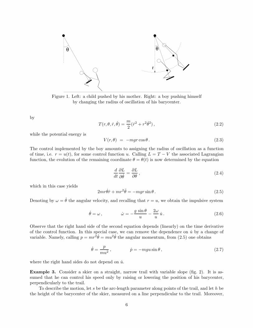
Example 1. Consider a small child riding on a swing, pushed by his mother. His motion is similarto that of a forced pendulum, say of length ℓ and mass m (see fig. 1, left). In addition to the gravityacceleration g, the child is subject to a force F = u(t) exerted by the pushing parent. This forcerepresents a control, and its value can be prescribed at will (within certain bounds) as function oftime. Calling θ the angle with a vertical line, the motion of the swing is described by the equation

mℓθ = −mgℓ sin θ + u(t) . (2.1)

This is a control equation in standard (non-impulsive) form.

Example 2. Next, consider an older boy riding on the same swing. By standing up or kneelingdown, he can change at will the radius of oscillation (see fig. 1, right). We describe this new systemin terms of two variables: the angle θ and the radius of oscillation r. The kinetic energy is given

5

r

θθ

Figure 1. Left: a child pushed by his mother. Right: a boy pushing himselfby changing the radius of oscillation of his barycenter.

by

T (r, θ, r, θ) =m

2(r2 + r2θ2) , (2.2)

while the potential energy isV (r, θ) = −mgr cos θ . (2.3)

The control implemented by the boy amounts to assigning the radius of oscillation as a functionof time, i.e. r = u(t), for some control function u. Calling L = T − V the associated Lagrangianfunction, the evolution of the remaining coordinate θ = θ(t) is now determined by the equation

d

dt

∂L

∂θ=∂L

∂θ, (2.4)

which in this case yields2mrθr +mr2θ = −mgr sin θ . (2.5)

Denoting by ω = θ the angular velocity, and recalling that r = u, we obtain the impulsive system

θ = ω , ω = −g sin θ

u− 2ω

uu . (2.6)

Observe that the right hand side of the second equation depends (linearly) on the time derivativeof the control function. In this special case, we can remove the dependence on u by a change ofvariable. Namely, calling p = mr2θ = mu2θ the angular momentum, from (2.5) one obtains

θ =p

mu2, p = −mgu sin θ , (2.7)

where the right hand sides do not depend on u.

Example 3. Consider a skier on a straight, narrow trail with variable slope (fig. 2). It is as-sumed that he can control his speed only by raising or lowering the position of his barycenter,perpendicularly to the trail.

To describe the motion, let s be the arc-length parameter along points of the trail, and let h bethe height of the barycenter of the skier, measured on a line perpendicular to the trail. Moreover,

6

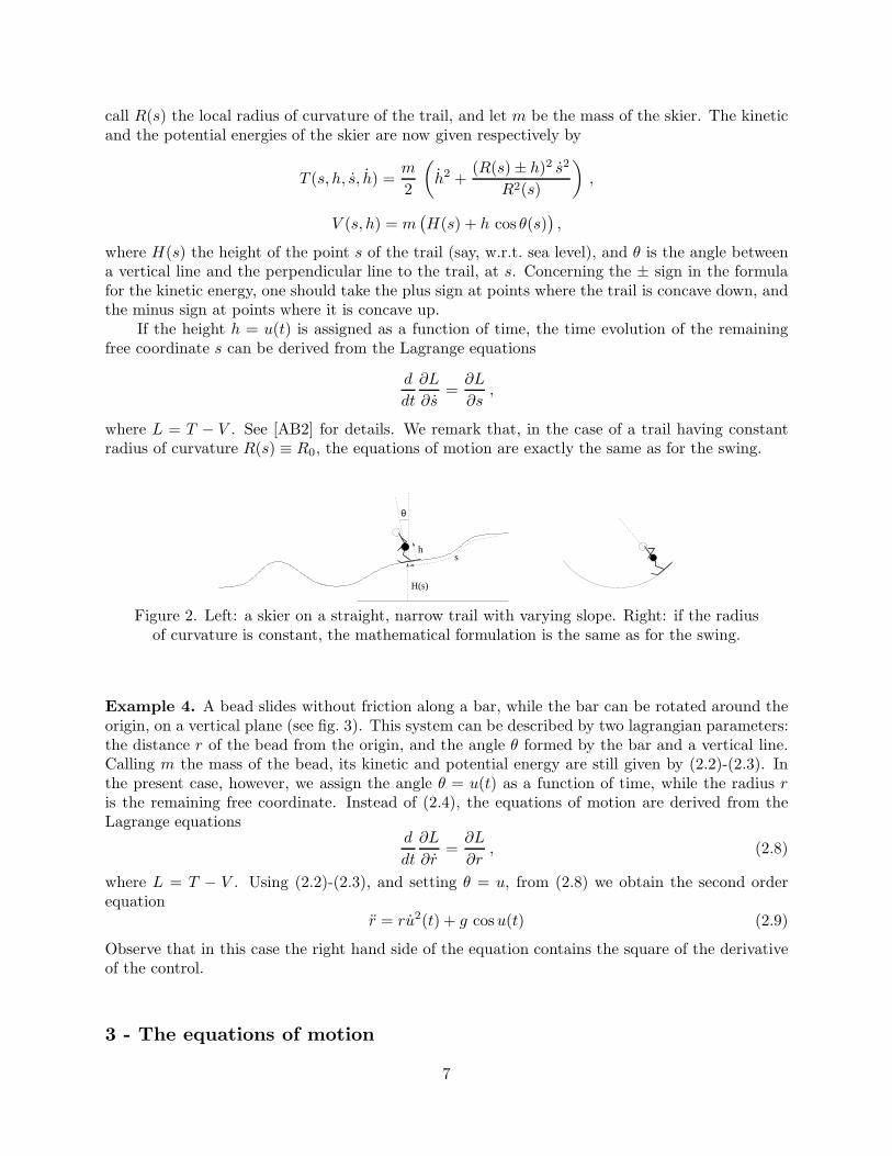
call R(s) the local radius of curvature of the trail, and let m be the mass of the skier. The kineticand the potential energies of the skier are now given respectively by

T (s, h, s, h) =m

2

(h2 +

(R(s) ± h)2 s2

R2(s)

),

V (s, h) = m(H(s) + h cos θ(s)

),

where H(s) the height of the point s of the trail (say, w.r.t. sea level), and θ is the angle betweena vertical line and the perpendicular line to the trail, at s. Concerning the ± sign in the formulafor the kinetic energy, one should take the plus sign at points where the trail is concave down, andthe minus sign at points where it is concave up.

If the height h = u(t) is assigned as a function of time, the time evolution of the remainingfree coordinate s can be derived from the Lagrange equations

d

dt

∂L

∂s=∂L

∂s,

where L = T − V . See [AB2] for details. We remark that, in the case of a trail having constantradius of curvature R(s) ≡ R0, the equations of motion are exactly the same as for the swing.

θ

h

H(s)

s

Figure 2. Left: a skier on a straight, narrow trail with varying slope. Right: if the radiusof curvature is constant, the mathematical formulation is the same as for the swing.

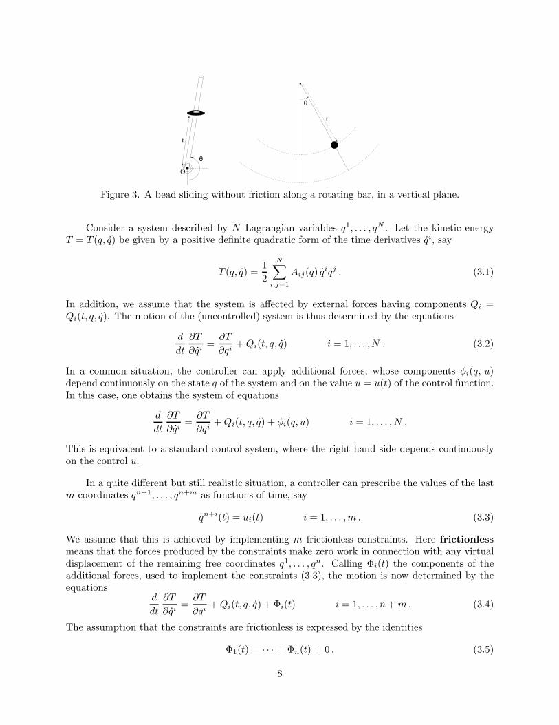
Example 4. A bead slides without friction along a bar, while the bar can be rotated around theorigin, on a vertical plane (see fig. 3). This system can be described by two lagrangian parameters:the distance r of the bead from the origin, and the angle θ formed by the bar and a vertical line.Calling m the mass of the bead, its kinetic and potential energy are still given by (2.2)-(2.3). Inthe present case, however, we assign the angle θ = u(t) as a function of time, while the radius ris the remaining free coordinate. Instead of (2.4), the equations of motion are derived from theLagrange equations

d

dt

∂L

∂r=∂L

∂r, (2.8)

where L = T − V . Using (2.2)-(2.3), and setting θ = u, from (2.8) we obtain the second orderequation

r = ru2(t) + g cosu(t) (2.9)

Observe that in this case the right hand side of the equation contains the square of the derivativeof the control.

3 - The equations of motion

7

θ

O

θ

r

r

Figure 3. A bead sliding without friction along a rotating bar, in a vertical plane.

Consider a system described by N Lagrangian variables q1, . . . , qN . Let the kinetic energyT = T (q, q) be given by a positive definite quadratic form of the time derivatives qi, say

T (q, q) =1

2

N∑

i,j=1

Aij(q) qiqj . (3.1)

In addition, we assume that the system is affected by external forces having components Qi =Qi(t, q, q). The motion of the (uncontrolled) system is thus determined by the equations

d

dt

∂T

∂qi=∂T

∂qi+Qi(t, q, q) i = 1, . . . ,N . (3.2)

In a common situation, the controller can apply additional forces, whose components φi(q, u)depend continuously on the state q of the system and on the value u = u(t) of the control function.In this case, one obtains the system of equations

d

dt

∂T

∂qi=∂T

∂qi+Qi(t, q, q) + φi(q, u) i = 1, . . . ,N .

This is equivalent to a standard control system, where the right hand side depends continuouslyon the control u.

In a quite different but still realistic situation, a controller can prescribe the values of the lastm coordinates qn+1, . . . , qn+m as functions of time, say

qn+i(t) = ui(t) i = 1, . . . ,m . (3.3)

We assume that this is achieved by implementing m frictionless constraints. Here frictionlessmeans that the forces produced by the constraints make zero work in connection with any virtualdisplacement of the remaining free coordinates q1, . . . , qn. Calling Φi(t) the components of theadditional forces, used to implement the constraints (3.3), the motion is now determined by theequations

d

dt

∂T

∂qi=∂T

∂qi+Qi(t, q, q) + Φi(t) i = 1, . . . , n+m. (3.4)

The assumption that the constraints are frictionless is expressed by the identities

Φ1(t) = · · · = Φn(t) = 0 . (3.5)

8

Remarkably, there is no need to compute the remaining components of the forces Φn+1 , . . . ,Φn+m,in order to completely determine the evolution of the system. Indeed, the variables qn+1, . . . , qn+m

are already assigned by (3.3). Of course, their time derivatives

qn+1 = u1(t) , . . . , qn+m = um(t)

are also determined. We now show that the evolution of components q1, . . . , qn can be derivedfrom the first n equations in (3.4), taking (3.5) into account. This is done in two steps.

STEP 1: In connection with the quadratic form (3.1), introduce the conjugate moments

pi = pi(q, q).=

∂T

∂qi=

n+m∑

i=1

Aij(q) qj . (3.6)

Moreover, define the Hamiltonian function

H(q, p) =1

2

n+m∑

i,j=1

Bij(q) pipj , (3.7)

where Bij are the components of the (n+m)× (n+m) inverse matrix B = A−1. In other words,

n+m∑

j=1

BijAjk =

1 if i = k,0 if i 6= k.

(3.8)

STEP 2: Solve the system of Hamiltonian equations for the first n variables

qi =∂H

∂pi(q, p)

pi = −∂H∂qi

(q, p) +Qi(t, q, q)

i = 1, . . . , n . (3.9)

Notice that (3.9) is a system of 2n equations for q1, . . . , qn, p1, . . . , pn, where the right hand sidealso depends on the remaining components qi, pi, i = n+1, . . . , n+m. We can remove this explicitdependence by inserting the values

qn+i = ui(t) , qn+i = ui(t) i = 1, . . . ,m ,

pj = pj(p1, . . . , pn, qn+1, . . . , qn+m) j = n+ 1, . . . , n+m.

(3.10)

In (3.10), to express pj as a linear combinations of p1, . . . , pn, qn+1, . . . , qn+m, we proceed as follows.

Let C = (Cij) be the inverse of the m×m submatrix (Bij)i,j=n+1,...,n+m, so that

n+m∑

i=n+1

CjiBik =

1 if j = k,0 if j 6= k,

j, k ∈ n+ 1, . . . , n+m . (3.11)

Recalling that p = Aq, q = Bp, we multiply by Cji both sides of the identity

qi =n∑

k=1

Bikpk +n+m∑

k=n+1

Bikpk ,

9

then we sum over i = n+ 1, . . . , n+m. By (3.11), this yields

pj =

n+m∑

i=n+1

Cjiqi −

n+m∑

i=n+1

n∑

k=1

CjiBikpk j = n+ 1, . . . , n+m. (3.12)

Inserting in (3.9) the values pn+1, . . . , pn+m given at (3.12), we obtain a closed system of 2nequations for the 2n variables q1, . . . , qn, p1, . . . , pn.

We now take a closer look at the equation of motion derived at (3.9)-(3.10). For simplicity,we temporarily assume that there are no external forces, i.e. Qi(t, q, q) ≡ 0. The extension to thegeneral case is straightforward.

Fix an index i ∈ 1, . . . , n. Inserting the values (3.12) for the last m components in (3.9) andrecalling the definition of the Hamiltonian function at (3.7), we obtain

qi =∂

∂pi

1

2

n+m∑

j,k=1

Bjk(q) pjpk

=n∑

j=1

Bij pj +n+m∑

j=n+1

Bij pj

=n∑

j=1

Bij pj +n+m∑

j=n+1

Bij

(n+m∑

ℓ=n+1

Cjℓ qℓ −

n+m∑

ℓ=n+1

n∑

k=1

CjℓBℓkpk

).

(3.13)

Next, using again (3.7) and (3.12) we compute

pi = − ∂

∂qi

1

2

n+m∑

j,k=1

Bjk(q) pjpk

= −

1

2

n∑

j,k=1

+n∑

j=1

n+m∑

k=n+1

+1

2

n+m∑

j,k=n+1

∂Bjk

∂qipjpk

= −1

2

n∑

j,k=1

∂Bjk

∂qipjpk −

n∑

j=1

n+m∑

k=n+1

∂Bjk

∂qipj

(n+m∑

h=n+1

Ckhqh −

n+m∑

h=n+1

n∑

ℓ=1

CkhBhℓpℓ

)

− 1

2

n+m∑

j,k=n+1

∂Bjk

∂qi

(n+m∑

h=n+1

Cjhqh −

n+m∑

h=n+1

n∑

ℓ=1

CjhBhℓpℓ

)(n+m∑

r=n+1

Ckr qr −

n+m∑

r=n+1

n∑

ℓ=1

CkrBrℓpℓ

).

(3.14)Recalling that qn+i = ui, and that the matrices C(q) =

(Cij(q)

)are invertible, a direct

inspection of the above equations reveals that:

(i) The right hand side of (3.13) is always an affine function of the derivatives u1 , . . . , um .

(ii) The right hand side of (3.14) is an affine function of the derivatives u1 , . . . , um if and only if

∂Bjk(q)

∂qi≡ 0 for all i ∈ 1, . . . , n , j, k ∈ n+ 1, . . . , n+m . (3.15)

10

Following [AB1], systems whose equations of motion are affine w.r.t. the time derivatives ofthe control will be called fit for jumps. In the special case where the derivatives ui do not appearat all in the equations, we say that the system is strongly fit for jumps. From the above analysiswe thus obtain

Theorem 1. The system described by (3.3)–(3.5) is “fit for jumps” if and only if the externalforces Qi are affine functions of the derivatives qj , j = n+ 1, . . . , n+m, and the identities (3.15)hold.

Theorem 2. The system at (3.3)–(3.5) is “strongly fit for jumps” provided that the external forcesQi depend only on the variables t, qi, and moreover the identities (3.15) hold, together with

Bij(q) ≡ 0 i ∈ 1, . . . , n , j ∈ n+ 1, . . . , n+m . (3.16)

4 - Geometric properties of the foliation

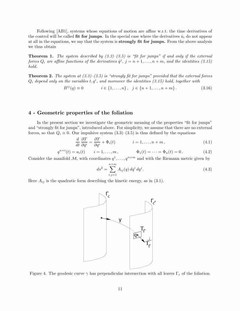
In the present section we investigate the geometric meaning of the properties “fit for jumps”and “strongly fit for jumps”, introduced above. For simplicity, we assume that there are no externalforces, so that Qi ≡ 0. Our impulsive system (3.3)–(3.5) is thus defined by the equations

d

dt

∂T

∂qi=∂T

∂qi+ Φi(t) i = 1, . . . , n+m, (4.1)

qn+i(t) = ui(t) i = 1, . . . ,m , Φ1(t) = · · · = Φn(t) = 0 . (4.2)

Consider the manifold M, with coordinates q1, . . . , qn+m and with the Riemann metric given by

ds2 =n+m∑

i,j=1

Aij(q) dqi dqj . (4.3)

Here Aij is the quadratic form describing the kinetic energy, as in (3.1).

ΓcΓc’

γ

TΓ

TΓ

q

Figure 4. The geodesic curve γ has perpendicular intersection with all leaves Γc of the foliation.

11

By assigning m constant values for the last m coordinates, say c1, . . . , cm, we obtain an n-dimensional submanifold

Γc.=(q1, . . . , qn+m) ; qn+1 = c1, · · · , qn+m = cm

. (4.4)

The union of all these submanifolds constitutes a foliation F of the original manifold M. Theanalysis in [AB1] and [Ra] has shown that the geometric properties of this foliation play a crucialrole in determining the form of the equations of motion (3.9)-(3.10). We summarize here the mainresults. Consider the following two properties:

(P1) If a geodesic curve γ crosses orthogonally one of the leaves Γc of the foliation F , then all ofthe other leaves touched by γ will also be crossed orthogonally.

(P2) The m-dimensional distribution T⊥Γ orthogonal to the leaves of the foliation is involutive.

The first property is illustrated in fig. 4. We now explain the second property. At each pointq ∈ M, the (n + m)-dimensional tangent space TM(q) can be decomposed as a direct sum (seefig. 5)

TM(q) = TΓ(q) ⊕ T⊥Γ (q) . (4.5)

Here TΓ(q) is the n-dimensional space tangent to the leaf of the foliation passing through q, whileT⊥

Γ (q) is its orthogonal complement, w.r.t. the metric (4.3).

γΤ

Γ⊥

Γc

(q , q ) = const.2 3

q = const.1

(q , q ) = const.2 3

ΓΤ⊥

Γ b

cΓ

ΓΤ

Figure 5. The distribution orthogonal to the leaves of the foliation Fcan be integrable (right) or not integrable (left).

The requirement that the distribution T⊥Γ is involutive means that, at least locally, it is

integrable (see fig. 5, right). One can thus find a system of adapted coordinates, which we still call(q1, . . . , qn+m), such that

TΓ(q) = span ∂

∂q1, . . . ,

∂

∂qn

, T⊥

Γ (q) = span ∂

∂qn+1, . . . ,

∂

∂qn+m

. (4.6)

12

Because of (4.6), for each choice of the constants b1, . . . , bn, the submanifold

Γb .=

(q1, . . . , qn+m) ; q1 = b1, · · · , qn = bn

. (4.7)

has a perpendicular crossing with every leaf Γc of the foliation F , defined at (4.4). Notice that thisorthogonality condition implies that, in the adapted coordinates, the symmetric matrix A = (Aij)defining the Riemann metric takes the form

A =

(A1 00 A2

),

where A1 is an n×n matrix, while A2 is an m×m matrix. In this case, the inverse matrix B = A−1

has the form

B = A−1 =

(A−1

1 00 A−1

2

),

hence the identities (3.16) clearly hold.

The main results, relating the form of the impulsive equations (4.1)-(4.2) to the geometricproperties of the foliation F in (4.4), are as follows.

Theorem 3. The impulsive system (4.1)-(4.2) is “fit for jumps” if and only if the foliation Fdefined at (4.4) satisfies the property (P1).

Theorem 4. Assume that the foliation F defined at (4.2) satisfies both properties (P1) and (P2).Then, in the adapted coordinates satisfying (4.6), the system (4.1)-(4.2) is “strongly fit for jumps”.

For a proof we refer to [Ra]. We remark that, in the case where the control is scalar (i.e.m = 1), the orthogonal distribution T⊥

Γ is always involutive. Therefore, if property (P1) is satisfied,one can construct a local system of coordinates satisfying (4.6), and the conclusion of Theorem 4holds.

θ = const.

Γc

θ

γ

r = const.

Γc

γ

θ

q

q

Figure 6. Left: a foliation satisfying the property (P1). Right: a foliation for which (P1) fails.

Theorem 3 is best illustrated by our earlier examples. In Example 2 (boy on a swing), we takethe radius of oscillation as controlled coordinate. The foliation whose leaves are the circumferences

Γc =

(r, θ) ; r = c

13

satisfies the property (P1). Indeed, in this case the geodesics are straight lines. If a straight lineγ crosses any of the circumferences Γc perpendicularly, then it still crosses perpendicularly all theothers (fig. 6, left). Hence the system is fit for jumps.

In Example 4 (bead sliding along a rotating axis), we consider a system with the same kineticenergy. However, we take the angle as a controlled coordinate. The foliation whose leaves are therays through the origin

Γc =

(r, θ) ; θ = c

does not satisfy the property (P1). A geodesic γ can cross one of the leaves perpendicularly ata point q, without crossing perpendicularly the other leaves Γc of the foliation (fig. 6, right). Inaccordance with Theorem 3, this system is not fit for jumps. Indeed, the equation of motion (2.9)contains the square of the time derivative of the control function.

The invariant character of the equations of motion was already pointed out in [Ma]. In otherwords, the motion depends only on the Riemannian metric tensor Aij and on the foliation F itself,not on the particular choice of coordinates which define the foliation.

In particular, recalling (3.14), consider the quadratic mapping Q = (Q1, . . . ,Qn), with

Qi(ξ1, . . . , ξm) = −1

2

n+m∑

j,k=n+1

∂Bj,k

∂qi

(m∑

h=1

Cj,n+hξh

)(m∑

r=1

Ck,n+rξr

), (4.8)

which describes the contribution of the quadratic terms qn+iqn+j = uiuj to the dynamics of thesystem. The intrinsic meaning of this quadratic mapping Q can be illustrated by the followingconstruction (fig. 7, left).

Let M be a Riemannian manifold of dimension n + m, where the metric is defined by thequadratic tensor Aij in (4.3). Consider a foliation F , with leaves Γc, which in a suitable coordinatesystem are described by (4.4). Notice that each leaf has dimension n, while the quotient manifoldM/F has dimension m.

Fix a point q, say on the leaf Γc. Observe that there is a canonical bijection between thetangent space TM/F (Γc) and the space T⊥

Γ (q) of tangent vectors v ∈ T (q) at the point q which areperpendicular to the leaf Γc.

For a given vector v ∈ T⊥Γ (q), construct the geodesic curve γ, which is tangent to v at q. For

a given ε > 0, let qε be the point on the curve γ which has distance ε |v| from q. This point willbe on some other leaf of the foliation, say qε ∈ Γc(ε) .

Next, construct a second geodesic curve γ′, starting from qε, which is perpendicular to the leafΓc(ε) and crosses the original leaf Γc at some point q′ε. For ε sufficiently small, using the implicitfunction theorem one can show that this second curve is unique. The limit

Q(v).= lim

ε→0

q′ε − q

ε2(4.9)

now defines a tangent vector at q. More precisely, the assignment v 7→ Q(v) is a homogeneousquadratic mapping from the space T⊥

Γ (q) of vectors perpendicular to the leaf Γc to the space TΓ(q)of vectors parallel to the leaf. We can extend this mapping to a symmetric bilinear form

T⊥Γ (q) ⊗ T⊥

Γ (q) 7→ TΓ(q)

by setting⟨v , w

⟩ .=

1

4

[Q(v + w) −Q(v −w)

].

14

Τ ⊥Γ

q

’εq

γ

γ’

Γc

Γc(ε)

cΓ

γ

qε

Τ⊥Γ

Figure 7. Left: construction of the quadratic mapping Q : T⊥Γ (q) 7→ Tγ(q).

Right: A curve γ orthogonal to all the hyper-surfaces Γc.

The expression (4.8) corresponds to this quadratic mapping, in a suitable set of coordinates. Fordetails of this construction, we refer to the forthcoming paper [BR5].

Two special cases of this construction are worth mentioning.

(I) If the system is “fit for jumps”, then by the property (P1) the geodesic γ is perpendicular tothe leaf Γc(ε) at the point qε. This implies γ′ = γ and hence q′ε = q for every ε. Hence Q ≡ 0.

(II) Let M = IRn+1 with the Euclidean metric. Assume that m = 1, so that the leaves of thefoliation are n-dimensional hypersurfaces. Then the orthogonal space T⊥

Γ (q) is 1-dimensional.The mapping Q is now defined in terms of the principal curvature of the curves γ orthogonalto the leaves Γc of the foliation (fig. 7, right). This case was studied in detail in [LR].

5 - Continuity of the control-to-trajectory map

Consider the Cauchy problem for the impulsive control system

x = f(t, x, u) +

m∑

i=1

gi(t, x, u) ui +

m∑

i,j=1

hij(t, x, u) uiuj , (5.1)

with initial data

x(0) = x , u(0) = u . (5.2)

Assume that all functions f, gi, hij are smooth. If the control function t 7→ u(t) is C1, then the localexistence and uniqueness of a solution follows from classical O.D.E. theory. A natural questionnow is:

What is the most general class of control functions u(·) for which the corresponding trajectoryof (5.1)-(5.2) is well defined ?

The answer strongly depends on the form of the equations (5.1). For example, if the coefficientshij do not vanish, then the control components ui must be absolutely continuous and have a square

integrable derivative. On the other hand, if gi ≡ 0, hij ≡ 0, then the derivatives of the control

15

function do not enter at all in the equation, and a unique solution can be constructed for anybounded, measurable control u(·).

An interesting case, on which we shall focus the attention, is when the system (3.3)-(3.5) isfit for jumps, but not strongly fit. Renaming coordinates, this leads to a system of the form

x = f(x) +m∑

i=1

gi(x) ui , (5.3)

where the vector fields gi do not commute, i.e. their Lie brackets [gi, gj ] do not vanish identically.In this setting, an appropriate class of control functions, for which a solution of (5.3)-(5.2) can bedefined, appears to be the space BV of functions with bounded variation. However, some caremust be taken. Given a discontinuous control u ∈ BV , if the vector fields gi do not commute, onecan find two sequences of uniformly Lipschitz continuous controls, say u(ν), v(ν), ν ≥ 1, such that

u(ν)(0) = v(ν)(0) = u(0) , ‖u(ν) − u‖L1 → 0 , ‖v(ν) − u‖L1 → 0 ,

but the corresponding trajectories of (5.3)-(5.2) converge to different limits. This will be shown inExample 5. To unique determine a trajectory x(· , u) corresponding to a control u ∈ BV , one alsoneeds to specify the curve along which u is varied, at times of jumps. This leads to the concept of“graph completion”, discussed later in this section.

Example 5. Consider the impulsive system on IR2

(x1, x2) = (1, 0) u1 + (0, x1) u2.= g1(x) u1 + g2(x) u2 , (5.4)

with initial conditions

(x1, x2)(0) = (0, 0) , (u1, u2) = (0, 0) . (5.5)

Observe that in this case the vector fields g1, g2 do not commute. Indeed, their Lie bracket is[g1, g2] = (Dg2) g1 − (Dg1) g2 = (0, 1). Consider the discontinuous control function

(u1, u2)(t) =

(0, 0) if t < 1 ,(1, 1) if t > 1 .

(5.6)

In the L1 norm, we can approximate u by a sequence of Lipschitz continuous control functionsu(ν), defined as

(u(ν)1 , u

(ν)2 )(t) =

(0, 0) if t ∈ [0, 1 − 1/ν] ,(0, 1 + ν(t− 1)) if t ∈ [1 − 1/ν, 1] ,(ν(t− 1), 1) if t ∈ [1, 1 + 1/ν] ,(1, 1) if t ∈ [1 + 1/ν, 2] .

(5.7)

The corresponding Caratheodory solutions of the Cauchy problem (5.4)-(5.5) are computed as

(x1, x2)(t, u(ν)) =

(0, 0) if t ∈ [0, 1] ,(ν(t− 1), 0) if t ∈ [1, 1 + 1/ν] ,(1, 0) if t ∈ [1 + 1/ν, 2] .

(5.8)

16

As ν → ∞, the above sequence of trajectories converges (pointwise and in the L1 norm) to thelimit trajectory

(x1, x2)(t) =

(0, 0) if t ∈ [0, 1] ,(1, 0) if t ∈ ]1, 2] .

(5.9)

Next, consider a second approximating sequence

(v(ν)1 , v

(ν)2 )(t) =

(0, 0) if t ∈ [0, 1] ,(ν(t− 1), ν(t− 1)

)if t ∈ [1, 1 + 1/ν] ,

(1, 1) if t ∈ [1 + 1/ν, 2] .(5.10)

The corresponding solutions are now

(x1, x2)(t, v(ν)) =

(0, 0) if t ∈ [0, 1] ,(ν(t− 1), ν2(t− 1)2/2

)if t ∈ [1, 1 + 1/ν] ,

(1, 1/2) if t ∈ [1 + 1/ν, 2] .(5.11)

As ν → ∞, in this second case the limit trajectory is

(x1, x2)(t) =

(0, 0) if t ∈ [0, 1] ,(1, 1/2) if t ∈ ]1, 2] .

(5.12)

This limit is still well defined, but different from (5.9).

The above example shows that, in the non-commutative case, the limit of the approximatingtrajectories depends not only on the pointwise values of u, but also on the way we approximateu by more regular controls. Observe that in the first case the values of u(ν) change from (0,0) to(0,1), and then to (1,1). In the second case, the values of v(ν) vary from (0,0) directly to (1,1)along a straight line. This suggests that, in the noncommutative case, a unique trajectory can bedetermined only if, at every time τ where u has a jump, we specify along which path the transitionfrom u(τ−) to u(τ+) takes place. The next definition makes this more precise.

Definition 1. A graph-completion of a BV function u : [0, T ] 7→ IRm is a Lipschitz continuouspath γ = (γ0, γ1, . . . , γm) : [0, S] 7→ [0, T ] × IRm such that

(i) γ(0) = (0, u(0)), γ(S) = (T, u(T )),

(ii) γ0(s1) ≤ γ0(s2) for all 0 ≤ s1 < s2 ≤ S,

(iii) for each t ∈ [0, T ] there exists some s such that γ(s) = (t, u(t)).

Notice that the path γ provides a continuous parametrization of the graph of u in the (t, u)space. At a time τ where u has a jump, the curve γ must include an arc joining the left and rightpoints

(τ, u(τ−)

),(τ, u(τ+)

).

Remarks. If the function u itself is Lipschitz continuous, one can construct a graph completionof u simply by taking γ(s) =

(s , u(s)

).

If u is a BV function taking values in an Euclidean space, there is a canonical way to constructa graph completion. Namely:

STEP 1: Bridge each jump of u with a straight segment,

17

u2

1u

τ t

u(t)

γ

Figure 8. A graph completion of a BV function u with two jumps.

STEP 2: Reparametrize the entire curve by arc-length.

In the case where u takes values in a Riemann manifold, one could move from u(τ−) to u(τ+)along a geodesic (assuming that the shortest path connecting the two values is unique). In general,however, the choice of the specific path can only be justified case by case.

Using graph-completions, we can now construct generalized trajectories for impulsive controlsystems with non-commutative vector fields.

Consider again the impulsive Cauchy problem (5.3), (5.2). Let u : [0, T ] 7→ IRm be a controlfunction with bounded variation, and let γ = (γ0, γ1, . . . , γm) be a graph-completion of u. Considerthe related Cauchy problem

d

dsy(s) = f

(y(s)

)γ0(s) +

m∑

i=1

gi

(y(s)

)γi(s) , y(0) = x . (5.13)

Definition 2. Let y(·, γ) be the unique Caratheodory solution of (5.13). Then the (possiblymultivalued) function

t 7→ x(t, γ) = y(s, γ) ; γ0(s) = t

is the generalized trajectory of (5.2)-(5.3) determined by the graph-completion γ of u.

Observe that, by definition, the path γ is absolutely continuous, hence the Caratheodorysolution of (5.13) is well defined.

It can be shown that the trajectory x(·, γ) depends on the path γ itself, but not on the way it

is parametrized. In particular, let γ : [0, S] 7→ [0, T ] × IRm be another graph-completion of u suchthat

γ(s) = γ(φ(s)

)s ∈ [0, S]

for some absolutely continuous, strictly increasing φ : [0, S] 7→ [0, S]. Then the generalizedtrajectories x(·, γ) and x(·, γ) coincide.

Example 5 (continued). For the discontinuous function u in (5.6), consider the graph-completion

18

1u

1 2 t

γ

γ~

0

u

u(t)

2

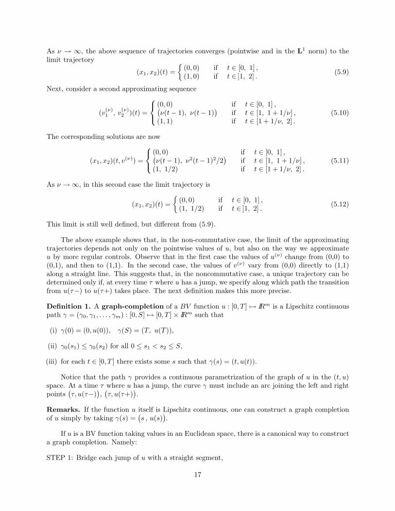
Figure 9. The curves γ and γ provide two different graph-completions of the same function u(·).

γ : [0, 4] 7→ [0, 2] × IR2 defined as (see fig. 9)

γ(s) =

(s, 0, 0) if s ∈ [0, 1] ,(1, 0, s− 1) if s ∈ [1, 2] ,(1, s− 2, 1) if s ∈ [2, 3] ,(s− 3, 1, 1) if s ∈ [3, 4] .

(5.14)

The generalized trajectory t 7→ x(t, γ) is

x(t, γ) =

(0, 0) if t ∈ [0, 1[ ,(1, 0) if t ∈]1, 2] ,

x(1, γ) =(ξ, 0) ; 0 ≤ ξ ≤ 1

.

(5.15)

Observe that the curve γ in this case is precisely the limit of the graphs of the approximatingfunctions u(ν) at (5.7). For all t ∈ [0, 2], t 6= 1, the generalized trajectory coincides with the limitin (5.9). At the time τ = 1 where u has a jump, the generalized trajectory x(1, γ) is multivalued.

A different graph-completion is achieved by bridging the jump at time τ = 1 with one singlestraight segment. This yields the path γ : [0, 3] 7→ [0, 2] × IR2 defined as (see fig. 9)

γ(s) =

(s, 0, 0) if s ∈ [0, 1] ,(1, s− 1, s− 1) if s ∈ [1, 2] ,(s− 1, 1, 1) if s ∈ [2, 3] .

(5.16)

The corresponding (multivalued) trajectory of (5.13) is given by

x(t, γ) =

(0, 0) if t ∈ [0, 1] ,(1, 1/2) if t ∈ [1, 2] ,

x(1, γ) =(ξ, ξ2/2) ; 0 ≤ ξ ≤ 1

.

(5.17)

In this case, the curve γ is the limit of the graphs of the approximating functions v(ν) at (5.10).For all t ∈ [0, 2], t 6= 1, the generalized trajectory coincides with the limit in (5.12), while x(1, γ)is multivalued.

It is important to understand how the trajectory of the system (5.13) depends on the choiceof graph completion. The main results in this direction, proved in [BR1], are as follows.

19

Let γ : [0, S] 7→ IR1+m and γ : [0, S] 7→ IR1+m be any two graph completions of the samecontrol function u ∈ BV . Define their distance as

∆(γ, γ).= inf

φmax

s∈[0,S]

∣∣∣γ(s) − γ(φ(s)

)∣∣∣ , (5.18)

where the infimum is taken over all continuous, strictly increasing, surjective maps φ : [0, S] 7→[0, S] . In addition, we recall that the Hausdorff distance between two compact sets A,B ⊂ IRN is

dH(A,B).= max

maxa∈A

d(a,B) , maxb∈B

d(b,A)

.

The distances of a point from a set are here defined as

d(a,B) = infx∈B

|x− a| , d(b,A) = infx∈A

|x− b| .

We then have

Theorem 5. Let the vector fields f, gi in (5.3) be Lipschitz continuous. Let un : [0, T ] 7→ IRm bea sequence of control functions. For each n ≥ 0, let γn be a graph-completion of un . Assume thatthe total variation of the maps γn remains uniformly bounded, and that

∆(γn , γ0) → 0 as n→ ∞ . (5.19)

Then the graphs of the corresponding (possibly multivalued) trajectories x(· , γn) converge to thegraph of x(· , γ0) in the Hausdorff metric.

For a proof, see [BR1]. The following result, also proved in [BR1], relates the generalizedsolution obtained from a graph completion to the limit of more regular solutions, corresponding tosmooth control functions.

Theorem 6. Let γ : [0, S] 7→ IR1+m be a graph completion of a control u : [0, T ] 7→ IRm. Let(un)n≥1 be a sequence of Lipschitz continuous controls with uniformly bounded total variation,which approximates γ in the following sense: setting γn(s)

.=(s, un(s)

), one has

∆(γ, γn) → 0 as n→ ∞ . (5.20)

Then the generalized solution x(· , γ) of (5.13) corresponding to the graph completion γ satisfies

x(t , γ) = limn→∞

x(t, un) (5.21)

at every time t where x(γ, t) is single valued, hence almost everywhere.

Example 5 (continued). The sequence of controls u(ν) at (5.7) approximates the graph comple-tion γ at (5.14). The corresponding trajectories x(· , u(ν)) converge pointwise to the generalizedtrajectory t 7→ x(t, γ) in (5.15), for every t 6= 1.

On the other hand the sequence of controls v(ν) at (5.10) approximates the graph completion γat (5.16). The corresponding trajectories x(· , v(ν)) converge pointwise to the generalized trajectoryt 7→ x(t, γ) in (5.17), for every t 6= 1.

20

6 - A related differential inclusion

We now consider a general control system where the right hand side is a linear or quadraticfunction of the derivative of the control:

x = f(x) +m∑

i=1

gi(x) ui +m∑

i,j=1

hij(x) uiuj . (6.1)

We always assume that all functions f , gi, and hij = hji are Lipschitz continuous. Given the initialconditions

x(0) = x , u(0) = u , (6.2)

for every smooth control function u : [0, T ] 7→ IRm one obtains a unique solution t 7→ x(t; u) ofthe Cauchy problem (6.1)-(6.2). More generally, since the equation (6.1) is quadratic w.r.t. thederivative u, it is natural to consider as set of admissible controls all the absolutely continuousfunctions u(·) with derivative in L2. For example

U .=u : [0, T ] 7→ IRm ;

∫ T

0

∣∣u(t)∣∣2 dt <∞

. (6.3)

In this connection, a natural problem is to describe the set of all admissible trajectories. Themain goal of the following analysis is to provide a characterization of the closure of this set oftrajectories, in terms of an auxiliary differential inclusion

It will be convenient to work in an extended the state space, and use the variable y =

(x0

x

)∈

IR1+n. For a given y, consider the set

F (y).= co

(1

f(x)

)v20 +

m∑

i=1

(0

gi(x)

)v0vi +

m∑

i,j=1

(0

hij(x)

)vivj ; v0 ≥ 0 ,

m∑

i=0

v2i = 1

.

(6.4)By co(A) we denote here the closed convex hull of a set A ⊂ IR1+n. Notice that the multifunctionF is Lipschitz continuous w.r.t. the Hausdorff metric [AC], and has convex, compact values. For agiven interval [0, S], the set of trajectories of the differential inclusion

y(s) ∈ F (y) , y(0) =

(0x

)(6.5)

is a non-empty, closed, bounded subset of C([0, S] ; IR1+n

). Consider one particular solution, say

s 7→ y(s) =

(x0(s)x(s)

), defined for s ∈ [0, S]. Assume that T

.= x0(S) > 0. Since the map s 7→ x0(s)

is non-decreasing, it admits a generalized inverse

s = s(t) if x0(s) = t . (6.6)

Indeed, for all but countably many times t ∈ [0, T ] there exists a unique value of the parameter ssuch that the identity on the right of (6.6) holds. We can thus define a corresponding trajectory

t 7→ x(t) = x(s(t)

)∈ IRn. (6.7)

21

This map is well defined for almost all times t ∈ [0, T ].

To establish a connection between the original control system (6.1) and the differential inclu-sion (6.5), consider first a smooth control function u : [0, T ] 7→ IRm. Define a reparametrized timevariable by setting

s(t).=

∫ t

0

(1 +

∑

i

u2i (τ)

)1/2

dτ . (6.8)

Notice that the map t 7→ s(t) is strictly increasing. The inverse map s 7→ t(s) is uniformly Lipschitzcontinuous and satisfies

dt

ds=

(1 +

∑

i

u2i (t)

)−1/2

.

Let now x : [0, T ] 7→ IRn be a solution of (6.1) corresponding to the smooth control u(·). We

claim that the map s 7→ y(s).=

(t(s)

x(t(s))

)is a solution to the differential inclusion (6.5). Indeed,

setting

v0(s).=

1(1 +

∑j u

2j

(t(s)

))1/2, vi(s)

.=

ui

(s(t)

)(1 +

∑j u

2j

(t(s)

))1/2i = 1, . . . ,m , (6.9)

one has

d

ds

t(s)

x(s)

=

v20(s)

f(x(s)

)v20(s) +

∑mi=1 gi

(x(s)

)v0(s)vi(s) +

∑mi,j=1 hij

(x(s)

)vi(s)vj(s)

.

Hence (6.5) holds, because by (6.9)m∑

i=0

v2i (s) ≡ 1 .

The following theorem shows that every solution of the differential inclusion (6.5) can beapproximated by smooth solutions of the original control system (6.1). More precisely, one canachieve: (i) convergence of trajectories in the space L1

([0, T ]

), and (ii) pointwise convergence at

the terminal time.

Theorem 7. Let y : [0, S] 7→ IR1+n be a solution to the multivalued Cauchy problem (6.5). Let thefirst component satisfy x0(S) = T > 0. Then there exists a sequence of smooth control functionsu(ν) : [0, T ] 7→ IRm such that the following properties hold.

(i) Define the rescaled time t 7→ sν(t) as in (6.8), call s 7→ tν(s) the inverse map and set xν(s).=

x(tν(s) , u(ν)

). Here t 7→ x(t, u(ν)) is the solution of (6.1)-(6.2) using the control u(ν). Then

one has

u(ν)(0) = u , sν(T ) = S for all ν ≥ 1 . (6.10)

Moreover, the corresponding solutions s 7→(tν(s)xν(s)

)converge to the map s 7→ y(s) uniformly

on [0, S].

22

(ii) Defining the rescaled time t 7→ s(t) as in (6.6) and setting

(t

x(t)

)= y(s(t)), we have

limν→∞

x(T, u(ν)) = x(T ) , limν→∞

∫ T

0

∣∣x(t) − xν(t)∣∣ dt = 0 . (6.11)

Proof. By assumptions, the extended vector fields

f =

(1f

), gi =

(0gi

), hij =

(0hij

)

are Lipschitz continuous. Consider the set of trajectories of the control system on IR1+n

d

dsy(s) = f v2

0 +m∑

i=1

gi v0vi +m∑

i,j=1

hji vivj , y(0) =

(0x

), (6.12)

where the controls vi satisfy the constraints

v0(s) ∈ [0, 1] ,

m∑

i=0

v2i (s) = 1 s ∈ [0, S] .

In the above setting, it is well known that the set of trajectories of (6.12) is dense on the setof solutions of the differential inclusion (6.5). In particular, there exists a sequence of control

functions s 7→ v(ν)(s) =(v(ν)0 , . . . , v

(ν)m

)(s), ν ≥ 1, such that the corresponding solutions s 7→

y(ν)(s) = y(s, v(ν)) of (6.12) converge to y(·) uniformly for s ∈ [0, S]. Notice that this implies

y(ν)0 (S) =

∫ S

0

(v(ν)0 )2(s) ds→ y0(S) = T . (6.13)

We now observe that the “input-output map” v(·) 7→ y(·, v) from controls to trajectoriesis uniformly continuous as a map from L1

([0, S] ; IR1+m

)into C

([0, S] ; IR1+n

). Thanks to the

assumption x0(S) = T > 0, we can slightly modify the controls v(ν) in L1 and replace the sequencev(ν) by a new sequence of smooth control functions w(ν) : [0, S] 7→ IR1+m with the followingproperties:

w(ν)0 (s) > 0 for all s ∈ [0, S] , ν ≥ 1 . (6.14)

∫ S

0

(w

(ν)0 (s)

)2ds = T for all ν ≥ 1 , (6.15)

limν→∞

∫ S

0

∣∣w(ν)(s) − v(ν)(s)∣∣ds = 0 . (6.16)

This implies the uniform convergence

y(·, w(ν)) =

(x0(·, w(ν))x(·, w(ν))

)→ y(·)

23

in C([0, S] ; IR1+n

). In particular, looking at the last n coordinates, we have

limν→∞

∥∥x(·, w(ν)) − x(·)∥∥C([0,S])

= 0 (6.17)

By (6.14), for each ν ≥ 1 the map

s 7→ x0(s, w(ν))

.=

∫ s

0

[w

(ν)0 (ξ)

]2dξ

is strictly increasing. Therefore it has a smooth inverse s = sν(t) We now define the sequence of

smooth control functions u(ν) =(u

(ν)1 , . . . , u

(ν)m

)from [0, T ] into IRm by setting

u(ν)i (t) =

w(ν)i (sν(t))

w(ν)0 (sν(t))

t ∈ [0, T ] . (6.18)

By construction, the corresponding solutions x(· , u(ν)) of (6.1) coincide with the trajectories con-structed above, namely:

x(t, u(ν)) = x(sν(t) , w(ν)

)t ∈ [0, T ] . (6.19)

Because of (6.17), this implies

limν→∞

(sup

s∈[0,S]

∣∣x(tν(s) , u(ν)) − x(s)∣∣)

= 0 . (6.20)

Next, by (6.15) we have tν(S) = T for every ν. Therefore, the first limit in (6.11) is animmediate consequence of (6.20).

To establish the second limit in (6.11), let t(s).= x0(s) be the first coordinate of the map

s 7→ y(s), and denote by t 7→ s(t) its inverse, as in (6.6). For each ν ≥ 1, consider the maps 7→ tν(s) together with its inverse t 7→ sν(t). Notice that each sν is smooth. Moreover we have

∣∣∣∣d

dst(s)

∣∣∣∣ ≤ 1 ,

∣∣∣∣d

dstν(s)

∣∣∣∣ ≤ 1 , (6.21)

limν→∞

∫ T

0

∣∣s(t) − sν(t)∣∣ dt = lim

ν→∞

∫ S

0

∣∣t(s) − tν(s)∣∣ds = 0 . (6.22)

Using (6.19), and then (6.21) to ensure that |dt| ≤ |ds|, we obtain the estimate

∫ T

0

∣∣∣x(s(t)

)− x(t, u(ν))

∣∣∣ dt =

∫ T

0

∣∣∣x(s(t))− x(s(t) , w(ν))

∣∣∣ dt+

∫ T

0

∣∣∣x(s(t) , w(ν)

)− x(sν(t), w(ν)

)∣∣∣ dt

≤∫ S

0

∣∣x(s) − x(s, w(ν))∣∣ ds+ C ·

∫ T

0

∣∣s(t) − sν(t)∣∣ dt .

(6.23)Here the constant C denotes an upper bound for the derivative w.r.t. s, say,

C.= sup

x

∣∣f(x)

∣∣+∑

i

∣∣gi(x)∣∣+∑

ij

∣∣hij(x)∣∣ .

24

By (6.20) and (6.22), the right hand side of (6.23) vanishes as ν → ∞. This completes the proofof the theorem.

For further results on the closure of the set of trajectories of (6.1), we refer to [BR3], [BR4],[BR5]. In particular, for a system which is “fit for jumps”, as in (5.3), one can consider iterated Liebrackets of the vector fields g1, . . . , gm, for example [gi, gj ],

[gj , [gj , gk]

], . . . By a classical result

in geometric control theory [AS], [J], the set of solutions of (5.3) is dense on the set of solutionsfor the more general control system

x = f(x) +∑

α

Gα(x) vα .

As vector fields Gα one can take here any collection of iterated Lie brackets of the fields gi.

7 - Stabilization

Aim of this section is to review various concepts of stability for the quadratic impulsive system(6.1), and relate them to the weak stability of a differential inclusion.

Definition 3. We say that the impulsive system (6.1) is stabilizable at the point x† ∈ IRn

if, for every ε > 0 there exists δ > 0 such that the following holds. For every initial state xwith |x − x†| ≤ δ there exists a C1 control function t 7→ u(t) = (u1, . . . , um)(t) such that thecorresponding trajectory of (6.1)-(6.2) satisfies

|x(t, u) − x†| ≤ ε for all t ≥ 0 . (7.1)

We say that the system (6.1) is asymptotically stabilizable at the point x if a control u(·) canbe found such that, in addition to (7.1), the trajectory satisfies

limt→∞

x(t, u) = x† . (7.2)

Remark. In the above definition we are not putting any constraint on the control functionu : [0,∞[ 7→ IRm. In principle, one may well have |u(t)| → ∞ as t→ ∞. If one wishes to stabilizethe system (6.1) and at the same time keep the control values within a small neighborhood of agiven value u†, it suffices to consider the stabilization problem for an augmented system, addingthe variables xn+1, . . . , xn+m together with the equations

xn+j = uj j = 1, . . . ,m .

Similar stability concepts (see for example [Sm]) can be also defined for a differential inclusion

x ∈ F (x) . (7.3)

Definition 4. The point x† is weakly stable for the differential inclusion (7.3) if, for every ε > 0there exists δ > 0 such that the following holds. For every initial state x with |x − x†| ≤ δ thereexists a trajectory of (7.3) such that

x(0) = x , |x(t) − x†| ≤ ε for all t ≥ 0 . (7.4)

25

Moreover, x† is weakly asymptotically stable if, there exist a trajectory such that, in additionto (7.4), satisfy

limt→∞

x(t) = x† . (7.5)

There is an extensive literature, in the context of O.D.E’s, and of control systems or differentialinclusions, relating the stability of an equilibrium state to the existence of a Lyapunov function.We recall below the basic definition, in a form suitable for our applications. For simplicity, we shallconsider the case x = 0 ∈ IRn, which of course is not restrictive.

Definition 5. A scalar function V defined on a neighborhoodN of the origin is a weak Lyapunovfunction for the differential inclusion (7.3) if the following holds.

(i) V is continuous on N , and continuously differentiable on N \ 0.(ii) V (0) = 0 while V (x) > 0 for all x 6= 0,(iii) For every δ > 0 sufficiently small, the sublevel set x ; V (x) ≤ δ is compact.(iv) At each x 6= 0 one has

infy∈F (x)

∇V (x) · y ≤ 0 . (7.6)

In connection with the multifunction F defined at (6.4) we consider a second multifunctionF♦ obtained by projecting the sets F (y) ⊂ IR1+n into the subspace IRn. More precisely, we set

F♦(x).= co

f(x) v2

0 +

m∑

i=1

gi(x) v0vi +

m∑

i,j=1

hij(x) vivj ; v0 ≥ 0 ,

m∑

i=0

v2i = 1

. (7.7)

Observe that, if the vector fields f, gi , and hij are Lipschitz continuous, then the multifunctionF♦ is Lipschitz continuous with compact, convex values. The next result, proved in [BR5], relatesthe asymptotic stabilization of the impulsive system (6.1) to the stability of a related differentialinclusion.

Theorem 8. The impulsive system (6.1) is asymptotically stabilizable at the origin if and only ifthe origin is weakly asymptotically stable for the differential inclusion

d

dsx(s) ∈ F♦(x(s)) . (7.8)

The following result, also proved in [BR5], deals with the stabilization of the impulsive system(6.1), relying on the existence of a Lyapunov function.

Theorem 9. Assume that the differential inclusion (7.8) admits a Lyapunov function V = V (x)defined on a neighborhood N of the origin. More precisely, referring to the original multifunctionF at (6.4), assume that for every x ∈ N \ 0 there exists v = (v0, v) ∈ F (x) such that

∇V (x) · v ≤ 0 v0 > 0 . (7.9)

Then the quadratic impulsive system (6.1) can be stabilized at the origin.

Example 6. On R2, consider the constant vector fields f = (1, 0), h11 = (0, 1), h22 = (0,−1),g1 = g2 = h12 = h21 = (0, 0). Then, choosing v0 = 0, v1 = v2 = 1/

√2 in (7.7) we see that

26

(0, 0) ∈ F♦(x) for every x ∈ IR2. Hence the condition (7.6) is trivially satisfied by any functionV . However, it is clear that in this case the system (6.1) is not stabilizable at the origin. Thismotivates the stronger assumption (7.9) needed in the above theorem.

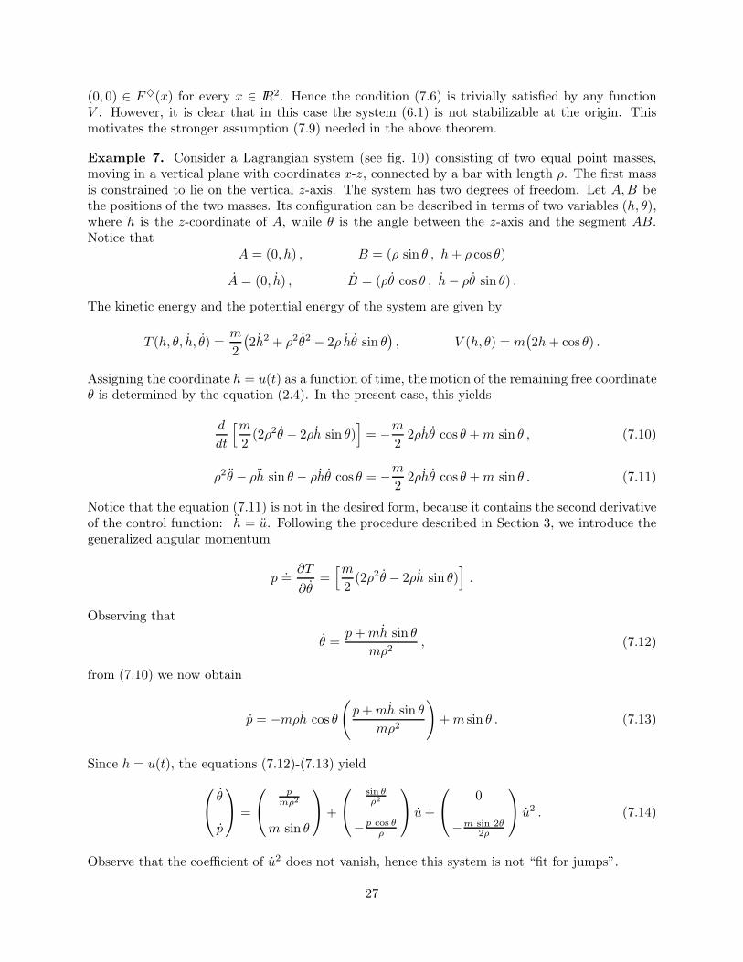
Example 7. Consider a Lagrangian system (see fig. 10) consisting of two equal point masses,moving in a vertical plane with coordinates x-z, connected by a bar with length ρ. The first massis constrained to lie on the vertical z-axis. The system has two degrees of freedom. Let A,B bethe positions of the two masses. Its configuration can be described in terms of two variables (h, θ),where h is the z-coordinate of A, while θ is the angle between the z-axis and the segment AB.Notice that

A = (0, h) , B = (ρ sin θ , h+ ρ cos θ)

A = (0, h) , B = (ρθ cos θ , h− ρθ sin θ) .

The kinetic energy and the potential energy of the system are given by

T (h, θ, h, θ) =m

2

(2h2 + ρ2θ2 − 2ρ hθ sin θ

), V (h, θ) = m

(2h+ cos θ) .

Assigning the coordinate h = u(t) as a function of time, the motion of the remaining free coordinateθ is determined by the equation (2.4). In the present case, this yields

d

dt

[m2

(2ρ2θ − 2ρh sin θ)]

= −m2

2ρhθ cos θ +m sin θ , (7.10)

ρ2θ − ρh sin θ − ρhθ cos θ = −m2

2ρhθ cos θ +m sin θ . (7.11)

Notice that the equation (7.11) is not in the desired form, because it contains the second derivativeof the control function: h = u. Following the procedure described in Section 3, we introduce thegeneralized angular momentum

p.=∂T

∂θ=[m

2(2ρ2θ − 2ρh sin θ)

].

Observing that

θ =p+mh sin θ

mρ2, (7.12)

from (7.10) we now obtain

p = −mρh cos θ

(p+mh sin θ

mρ2

)+m sin θ . (7.13)

Since h = u(t), the equations (7.12)-(7.13) yield

θ

p

=

pmρ2

m sin θ

+

sin θρ2

−p cos θρ

u+

0

−m sin 2θ2ρ

u2 . (7.14)

Observe that the coefficient of u2 does not vanish, hence this system is not “fit for jumps”.

27

Fix any angle θ, with |θ| < π/2. We claim that the above system can be asymptotically stabi-lized at the point (θ, 0). Indeed, according to Theorem 8, it suffices to show that the correspondingdifferential inclusion (7.8) is weakly asymptotically stable at (θ, 0).

Toward this goal, we observe that, by (7.14),

p

mρ2

m sin θ

∈ F♦(θ, p) ,

0

−m sin 2θ2ρ

∈ F♦(θ, p) . (7.15)

Therefore, since F♦ is convex, the set of trajectories of the differential inclusion (7.8) contains theset of all trajectories of the control system

d

ds

θ

p

=

p

mρ2

m sin θ

w(s) +

0

−m sin 2θ2ρ

(1 − w(s)), (7.16)

where the scalar control function s 7→ w(s) enters linearly. It now remains to check that (θ, 0) is anasymptotically stable equilibrium point for the system (7.16), provided that |θ| < π/2 . We workout details, assuming θ 6= 0.

w0.=

cos θ

ρ+ cos θ,

so that

w0 −cos θ

ρ(1 − w0) = 0 .

Notice that 0 < w0 < 1. In terms of the new control variable ω.= w − w0, the system (7.16) can

be rewritten as

d

ds

θ

p

=

pw0

mρ2

m(w0 − cos θ

ρ (1 − w0))

sin θ

+

pmρ2

m(1 + cos θ

ρ

)sin θ

ω(s) . (7.17)

where the control ω(s) now takes values in the interval [−w0 , 1 − w0]. Linearizing (7.17) at thepoint (θ, 0) we obtain the linear control system with constant coefficients

d

ds

θ − θ

p

=

0 w0

mρ2

m (1 − w0) sin2 θ 0

θ − θ

p

+

0

m(1 + cos θ

ρ

)sin θ

ω(s) . (7.18)

For |θ| < π/2, θ 6= 0, the linearized system (7.18) is completely controllable, hence (7.17) is locallyasymptotically stabilizable at the origin, as claimed. In the special case θ = 0, the proof thatthe two-dimensional system (7.16) is locally asymptotically controllable at the origin is somewhatmore lengthy. For a detailed analysis of planar control systems we refer to [BP].

28

θ

h

B

ρ

A

z

0 xFigure 10. This system can be stabilized at any angle θ < π/2, vibrating the point A up and down.

8 - Swim-like motion of bodies immersed in a fluid

In this section, we describe a further application of the theory of impulsive Lagrangian systems.Consider a body whose shape depends on a finite number of parameters q1, . . . , qN and is immersedin a homogeneous incompressible, non-viscous fluid.

To fix the ideas, let Ω ⊂ IRd be a reference configuration of the body. We assume that Ωis a bounded, open set with smooth boundary. The case where Ω consists of several connectedcomponents (modelling several bodies swimming in the same environment) is also of interest. Foreach given value q = (q1, . . . , qN ) of the Lagrangian parameters, let ξ 7→ ϕq(ξ) be a volumepreserving diffeomorphism. Assigning the coordinates q = q(t) as functions of time, the imageϕq(t)(Ω) thus describes the region of space occupied by the body at time t. Let

T (q, q) =N∑

i,j=1

Aij(q)qiqj (8.1)

describe the kinetic energy of the body. For simplicity, we assume that the surrounding fluid hasunit density. Calling v = v(x) its velocity at the point x, the kinetic energy of the surroundingfluid is given by

K =

∫

IRd\ϕq(Ω)

∣∣v(x)∣∣2

2dx . (8.2)

Ωqϕ (Ω)

ξ

ϕ (ξ)(ξ)n

qq

Figure 11. The reference configuration of the body, and the region occupied after a deformation.

29

For n + m = N , we assume that the last m Lagrangian coordinates qn+1, . . . , qn+m can beprescribed by a controller, as functions of time. As in (3.3), these assignments will be implementedby means of frictionless constraints. Assuming that no other forces are present, we wish to derivea system of equations describing the motion of the remaining n coordinates and of the surroundingfluid. Calling v = v(t, x) the fluid velocity, if the only active forces are due to the scalar pressurep, the motion is governed by the Euler equation for non-viscous, incompressible fluids:

vt + v · ∇v = −∇p , (8.3)

supplemented by the incompressibility condition

div v ≡ 0 . (8.4)

In addition, we need a boundary condition along ∂(ϕq(Ω)

)= ϕq(∂Ω), namely

⟨v(ϕq(ξ)

)−

n∑

i=1

∂

∂qϕq(ξ) · qi , nq(ξ)

⟩= 0 . (8.5)

Here nq(ξ) denotes the unit outer normal to the set ϕq(Ω) at the point ϕq(ξ).To find the evolution of the coordinates q1, . . . , qn, we observe that

d

dt

∂T

∂qi=∂T

∂qi+ Fi , (8.6)

where T is the kinetic energy of the body and Fi are the components of the external pressureforces, acting on the boundary of ϕq(Ω). To determine these forces, we observe that, in connectionwith a small displacement of the qi coordinate, the work done by the pressure forces is

δW = −δqi ·∫

∂Ω

⟨nq(ξ) ,

∂ϕq

∂qi(ξ)

⟩p(ϕq(ξ)

)Jq(ξ) dσ . (8.7)

Notice that the above integral is computed along the surface of the reference configuration. Thefactor Jq(ξ) gives the ratio between the area of an infinitesimal portion of the surface ϕq(∂Ω) andthe corresponding portion in the reference configuration ∂Ω. According to (8.6) and (8.7), theequation of motion for the first n coordinates is derived from

d

dt

∂T

∂qi=∂T

∂qi−∫

∂Ω

⟨nq(ξ) ,

∂ϕq

∂qi(ξ)

⟩p(ϕq(ξ)

)Jq(ξ) dσ . (8.8)

We now show that, in the case of irrotational flow, the coupled system of equations (8.3)–(8.5)and (8.8) can be reduced to a finite dimensional impulsive Lagrangian system. In particular, thetechniques discussed earlier in this paper can be applied to this situation as well.

To fix the ideas, we consider the two-dimensional case, assuming that the body has oneconnected component, and that the initial velocity of the fluid is irrotational with zero circulationaround the body. Since the flow is inviscid, this implies that vorticity and circulation will vanishidentically at all times.

For any given values of q = (q1, . . . , qN ), and q = (q1, . . . , qN ), consider the unique irrotationalvelocity field v = v(q,q) : IR2 \ ϕq(Ω) 7→ IR2 that satisfies the boundary conditions (8.5) and has

30

zero circulation around the body. It is well known [MP] that this velocity field can be computedby setting v = ∇ψ and solving the Neumann problem in the exterior domain

∆ψ = 0 x ∈ IR2 \ ϕq(Ω) , (8.9)

n · ∇ψ =N∑

i=1

n · ∂ϕq

∂qiqi x ∈ ∂ϕq(Ω) , (8.10)

∣∣ψ(x)∣∣→ 0 as |x| → ∞ . (8.11)

Call

T v(q, q).=

∫

IR2\ϕq(Ω)

∣∣v2(x)∣∣

2dx (8.12)

the kinetic energy of the fluid. Notice that this is entirely determined by q, q. For given valuesof q1, . . . , qN , the solution v(·) of the Neumann problem (8.9)–(8.11) depends linearly on theboundary conditions (8.10), hence it is a linear functional of the time derivatives qi, . . . , qN . Thekinetic energy in (8.12) is thus a quadratic function of these variables, say

T v(q, q).=

N∑

i,j=1

A′ij(q) q

iqj . (8.13)

Summing (8.1) with (8.13), we can now consider the total kinetic energy of the body and of thefluid:

T (q, q).= T (body) + T (fluid) =

N∑

i,j=1

Aij(q) qiqj +

N∑

i,j=1

A′ij(q) q

iqj . (8.14)

This achieves the desired reduction to a finite dimensional system.If the lastm coordinates are directly assigned as functions of time, say qn+1 = u1(t) , . . . , q

n+m =um(t) , the motion of the remaining n free coordinates q1, . . . , qn can be determined as in Section 3.

The only difference is that now we use T (q, q) as the total kinetic energy of the system.

References

[AM] R. Abraham and J. E. Marsden, Foundations of Mechanics. Benjamin/Cummings PublishingCo., Reading, Mass., 1978.

[AS] A. A. Agrachev and Y. L. Sachkov, Control Theory form the Geometric Viewpoint, Springer-Verlag, 2004.

[AC] J. P. Aubin and A. Cellina, Differential Inclusions. Springer-Verlag, Berlin, 1984.

[Ba] G. Barles, Deterministic impulse control problems. SIAM J. Control Optim. 23 (1985),419–432.

[BL] A. Bensoussan and J. L. Lions, Impulse Control and Quasivariational Inequalities. Heyden &Son, Philadelphia, 1984.

31

[BP] U. Boscain and B. Piccoli, Optimal Syntheses for Control Systems on 2-D Manifolds, SpringerSMAI series, Vol. 43, Heidelberg, 2004.

[B1] A. Bressan, On differential systems with impulsive controls, Rend. Semin. Mat. Univ. Padova78 (1987), 227-236.

[BR1] A. Bressan and F. Rampazzo, On differential systems with vector-valued impulsive controls,Boll. Un. Mat. Ital. 2-B (1988), 641-656.

[BR2] A. Bressan and F. Rampazzo, Impulsive control systems with commutative vector fields. J.Optim. Theory Appl. 71 (1991), 67–83.

[BR3] A. Bressan and F. Rampazzo, On differential systems with quadratic impulses and their ap-plications to Lagrangian mechanics. SIAM J. Control Optim. 31 (1993), 1205-1220.

[BR4] A. Bressan and F. Rampazzo, Impulsive control systems without commutativity assumptions.J. Optim. Theory Appl. 81 (1994), 435–457.

[BR5] A. Bressan and F. Rampazzo, Stabilization of Lagrangian systems by moving constraints, toappear.

[BR6] A. Bressan and F. Rampazzo, Impulsive control of Lagrangian systems with non-holonomicconstrains, to appear.

[AB1] Aldo Bressan, Hyper-impulsive motions and controllizable coordinates for Lagrangean systemsAtti Accad. Naz. Lincei, Memorie, Serie VIII, Vol. XIX (1990), 197–246.

[AB2] Aldo Bressan, On some control problems concerning the ski or swing, Atti Accad. Naz. Lincei,Memorie, Serie IX, Vol. I, (1991), 147-196.

[CF] F. Cardin and M. Favretti, Hyper-impulsive motion on manifolds. Dynam. Contin. DiscreteImpuls. Systems 4 (1998), 1–21.

[CWB] J. Carling, T. Williams, and G. Bowtell, Self-propelled anguilliform swimming: simultaneoussolutions of the two-dimensional Navier-Stokes equations and Newton’s laws of motion, J.Experimental Biology 201 (1998), 3143-3166.

[Ch] S. Childress, Mechanics of Swimming and Flying. Cambridge University Press, 1981.

[CM] A. J. Chorin and J. E. Marsden, A Mathematical Introduction to Fluid Mechanics. Springer-Verlag, New York, 1979.

[DM1] G. Dal Maso and F. Rampazzo, On systems of ordinary differential equations with measuresas controls. Differential Integral Equat. 4 (1991), 739–765.

[DM2] G. Dal Maso, P. LeFloch, and F. Murat, Definition and weak stability of nonconservativeproducts. J. Math. Pures Appl. (9) 74 (1995), 483–548.

[Ga] G. P. Galdi, On the motion of a rigid body in a viscous fluid: a mathematical analysis withapplications, in Handbook of Mathematical Fluid Dynamics, Vol.1, North-Holland, Amsterdam2002, pp.653-791.

32

[KMR] E. Kanso, J. E. Marsden, C. W. Rowley, and J. B. Melli-Huber, Locomotion of articulatedbodies in a perfect fluid. J. Nonlinear Sci. 15 (2005), 255–289.

[Ka1] P. L. Kapitsa, Dynamic stability of a pendulum when its point of suspension vibrates, Collectedworks by P. L. Kapitsa Vol. II, pp. 714-725. Pergamon Press, London, 1965.

[Ka2] P. L. Kapitsa, Pendulum with a vibrating suspension, Collected works by P. L. Kapitsa Vol.II, pp. 726-737. Pergamon Press, London, 1965.

[KM] S. D. Kelly and R. Murray, Modelling efficient pisciform swimming for control, Intern. J.Robust Nonlinear Control 201 (1998), 3143-3166.

[KO] V. V. Kozlov and D. A. Onishchenko, Motion of a body with undeformable shell and variablemass geometry in an unbounded perfect fluid, J. Dynam. Diff. Equat. 15 (2003), 553-570.

[KR1] V. V. Kozlov and S. M. Ramodanov, On the motion of a variable body in an ideal fluid, J.Appl. Math. Mech. 65 (2001), 579–587.

[KR2] V. V. Kozlov and S. M. Ramodanov, On the motion of a body with rigid shell and variablemass geometry in a perfect fluid, Doklady Physics 47 (2002), 132-135.

[KP] J. Kulkarni and B. Piccoli, Pumping a swing by standing and squatting: do children pumptime optimally? IEEE Control Systems Magazine 25 (2005), 8–56.

[J] V. Jurdjevic, Geometric Control Theory, Cambridge University Press, 1997.

[LF] P. LeFloch. Hyperbolic systems of conservation laws. The theory of classical and nonclassicalshock waves. Lectures in Mathematics ETH Zrich. Birkhuser, Basel, 2002.

[L1] M. Levi, Geometry and physics of averaging with applications, Physica D 132 (1999), 150-164.

[L2] M. Levi, Geometry of vibrational stabilization and some applications, Int. J. Bifurc. Chaos15 (2005), 2747-2756.

[LR] M. Levi and Q. Ren, Geodesics on vibrating surfaces and curvature of the normal family,Nonlinearity 18 (2005), 2737-2743.

[Lg] J. Lighthill, Mathematical biofluiddynamics, Society for Industrial and Applied Mathematics,Philadelphia, 1975.

[LS] W. S. Liu and H. J. Sussmann, Limits of highly oscillatory controls and the approximationof general paths by admissible trajectories, in Proc. 30-th IEEE Conference on Decision andControl, IEEE Publications, New York, 1991, pp. 437–442.

[Ma] C. Marle, Geometrie des systemes mecaniques a liaisons actives, in Symplectic Geometry andMathematical Physics, 260–287, P. Donato, C. Duval, J. Elhadad, and G. M. Tuynman Eds.,Birkhauser, Boston, 1991.

[MP] C. Marchioro and M. Pulvirenti, Mathematical Theory of Incompressible Nonviscous Fluids.Springer-Verlag, New York, 1994.

33

[M1] B. M. Miller, The generalized solutions of ordinary differential equations in the impulse controlproblems. J. Math. Systems Estim. Control 4 (1994).

[M2] B. M. Miller, Generalized solutions in nonlinear optimization problems with impulse controls.I. The problem of the existence of solutions. Automat. Remote Control 56 (1995), 505–516.

[M3] B. M. Miller, Generalized solutions in nonlinear optimization problems with impulse controls.II. Representation of solutions by means of differential equations with a measure. Automat.Remote Control 56 (1995), 657–669.

[MR] M. Motta and F. Rampazzo, Dynamic programming for nonlinear systems driven by ordinaryand impulsive controls. SIAM J. Control Optim. 34 (1996), 199–225.

[NS] H. Nijmeijer and A. van der Schaft, Nonlinear dynamical control systems, Springer-Verlag,New York, 1990.

[P] B. Piccoli, Time-optimal control problems for the swing and the ski, International Journal ofControl 62 (1995), 1409–1429.

[Ra] F. Rampazzo, On the Riemannian structure of a Lagrangean system and the problem of addingtime-dependent coordinates as controls European J. Mechanics A/Solids 10 (1991), 405-431.

[Re1] B. L. Reinhart, Foliated manifolds with bundle-like metrics. Annals of Math. 69 (1959),119-132.

[Re2] B. L. Reinhart, Differential geometry of foliations. The fundamental integrability problem.Springer-Verlag, Berlin, 1983.

[Sa] P. G. Saffman, The self-propulsion of a deformable body in a perfect fluid, J. Fluid Mech. 28(1967), 385-389.

[Sm] G. V. Smirnov, Introduction to the theory of differential inclusions, American MathematicalSociety, Graduate studies in mathematics, vol. 41 (2002).

[ST] J. San Martin, J. F. Scheid, T. Takahashi, and M. Tucsnak, An initial and boundary valueproblem modeling fish-like swimming, Arch. Rational Mech. Anal., to appear.

[St] A. Stephenson, On a new type of dynamical stability, Manchester Memoirs 52, (1908) 1-10.

[Su] H. J. Sussmann, On the gap between deterministic and stochastic ordinary differential equa-tions, Ann. Prob. 6 (1978), 17-41.

[Wu] T. Y. Wu, Mathematical biofluiddynamics and mechanophysiology of fish locomotion, Math.Methods Appl. Sci. 24 (2001), 1541-1564.

34