Improving Volumetric Sweep Efficiency in Enhanced Oil ...

Application of Fracturing Technology in Improving Volumetric Sweep Efficiency in Enhanced Oil Recovery Techniques

by

Elias Pirayesh, B.Sc.

A Thesis

In

PETROLEUM ENGINEERING

Submitted to the Graduate Faculty Of Texas Tech University in

Partial Fulfillment of the Requirements for

the Degree of

MASTER OF SCIENCE

Approved

Mohamed Soliman Chair of Committee

Habib Menouar

Shameem Siddiqui

Peggy Gordon Miller

Dean of the Graduate School

May, 2012

IN

PETROLEUM ENGINEERING

Texas Tech University, Elias Pirayesh, May 2012

ii

ACKNOWLEDGMENTS

This research would not have been accomplished without the help and support of

many people. I wish to express my sincere appreciation to my supervisor, Dr. Mohamed

Soliman who was profusely supportive and provided me with his insightful help and

guidance throughout my studies. Genuine gratitude is also to the members of the

supervisory committee, Dr. Shameem Siddiqui and Dr. Habib Menouar without whose

assistance, this work would not have been as fine as it is.

I would like to direct thanks to Halliburton Services for providing me with their

simulator Quiklook ©.

I would like to express my love and gratefulness to my beloved family; for their

understanding and endless love, through the duration of my studies.


iii

TABLE OF CONTENTS

ACKNOWLEDGMENTS ............................................................................................ II

ABSTRACT ................................................................................................................. V

LIST OF TABLES ...................................................................................................... VI

TABLE OF FIGURES ............................................................................................... VII

I. INTRODUCTION ..................................................................................................... 1

1.1. Statement of the Problem ............................................................................................. 6

1.2. Objective of the Project ............................................................................................... 7

II. METHODS............................................................................................................... 9

2.1. First case: Edge Water Drive Reservoir ..................................................................... 10

2.2. Second Case: Line Drive Water Flooding Pattern ..................................................... 12

2.3. Third Case: Five Spot Water Flooding Pattern .......................................................... 14

2.4. Optimization .............................................................................................................. 14

2.4.1. Barrier-fracture Length ................................................................... 14 2.4.2. Barrier-fracture Location ................................................................ 16 2.4.3. Number of Barrier-fracture ............................................................. 17 2.4.4. Mobility Ratio ................................................................................. 19 2.4.5. Schedule of Barrier-Fracturing ....................................................... 19

2.5. Relative Permeability Modifier Filled Barriers ......................................................... 19

III. RESULTS ............................................................................................................. 22

3.1. First Case: Edge-water Drive ..................................................................................... 22

3.2. Second Case – Line Drive Water Flooding Pattern ................................................... 24

3.3. Third Case – Five Spot Water Flooding Pattern ........................................................ 27

3.4. Optimization Results .................................................................................................. 30

3.4.1. Barrier-Fracture Length .................................................................. 30 3.4.2. Barrier-Fracture Location ............................................................... 32 3.4.3. Number of Barrier-fractures ........................................................... 35 3.4.4. Effect of Mobility Ratio .................................................................. 39 3.4.5. Effect of Barrier-Fracturing Time ................................................... 43

3.5. Relative Permeability Modifier Barrier ..................................................................... 47

IV. CONCLUSIONS AND RECOMMENDATIONS ............................................... 49

4.1. Conclusions ................................................................................................................ 49

4.2. Recommendations ...................................................................................................... 50


iv

REFERENCES ........................................................................................................... 51

A. SENSITIVITY ANALYSIS: EFFECT OF GRIDDING ON SIMULATION

RESULTS ............................................................................................................. 53


v

ABSTRACT

The industry has developed methods to improve sweep efficiency during

Enhanced Oil Recovery processes. These methods include the use of certain

injection/production patterns, drilling horizontal and deviated wells, use of special

chemicals as well as inflow control devices (ICDs). The purpose of the first two methods

is to create an even movement of injection fluid across the reservoir. Special chemicals

have been used to divert the injected fluid to eliminate channeling and to improve sweep

efficiency. Inflow control devices have been used to delay water or gas breakthrough,

making possible a more efficient drainage of the reservoir while maximizing production

and recovery.

The technique presented in this work creates a mechanical barrier to flow by

introducing a fracture to the formation at a strategic location. This fracture is then filled

with a conformance fluid which eventually becomes impermeable to fluid flow. The

effects of various design parameters on the performance of barrier-fractures have been

investigated and the results are presented. These design parameters include barrier-

fracture length & location, number of barrier-fractures, mobility ratio and barrier creation

time. It is illustrated that the breakthrough time and potential productivity of producing

wells increase as a result of enhancing the volumetric sweep efficiency of hydrocarbons.

A second technique introduced in this work is creating a chemical barrier to flow

by injecting relative permeability modifying agents into created cracks in reservoir rock.

Injection of relative permeability modifying agents (RPM) into rock reduces the rock’s

water relative permeability to a fraction of its original value. An investigation of the fluid

flow aspects of RPM barriers revealed that in terms of improving recovery the

performance of these chemical barriers is weak and have a strong tendency to rely on

RPM properties. Therefore, they may not be suitable candidates for in-depth flow profile

modification.


vi

LIST OF TABLES

2. 1 Edge water synthetic case data ................................................................... 11

2. 2 Line drive reservoir boundaries .................................................................. 13

2. 3 Line drive synthetic case data ..................................................................... 13


vii

TABLE OF FIGURES

2.1 Edge water drive reservoir grid ............................................................... 10

2. 2 Edge water drive reservoir map ............................................................... 10

2. 3 Edge water drive reservoir map with a barrier-fracture ........................... 11

2. 4 Line drive reservoir map .......................................................................... 12

2. 5 Line drive reservoir layers ....................................................................... 13

2. 6 Five spot reservoir map............................................................................ 14

2. 7 Barrier-fracture length equal to 25% of reservoir length ......................... 15



2. 10 Barrier-fracture placed at the first quarter of the reservoir ...................... 16

2. 11 Barrier-fracture placed at the center of the reservoir ............................... 17

2. 12 Barrier-fracture placed at the third quarter of the reservoir ..................... 17

2. 13 A reservoir with two barrier-fractures ..................................................... 18

2. 14 A reservoir with three barrier-fractures ................................................... 18

2. 15 A reservoir with four barrier-fractures ..................................................... 18

2.16 Reservoir rock relative permeability curves. (a) Before RPM treatment (b)

After RPM treatment................................................................................................. 20

2.17 Barrier created by injection of RPM agents into a fracture ...................... 21

3. 1 Water breakthrough into the horizontal well with no barrier-fracture ....... 22

3. 2 Water breakthrough into the horizontal well in the presence of a barrier-

fracture ...................................................................................................................... 23

3. 3 Oil production in the presence and absence of a barrier-fracture .............. 23

3. 4 Water production in the presence and absence of a barrier-fracture ......... 24

3. 5 Water saturation distribution in the absence of a barrier-fracture ............. 25

3. 6 Water saturation distribution in the presence of a barrier-fracture ............ 25

3. 7 Cross sectional water saturation distribution in the presence of a barrier-

fracture ...................................................................................................................... 26

3. 8 Oil production in the presence and absence of a barrier-fracture .............. 26


viii

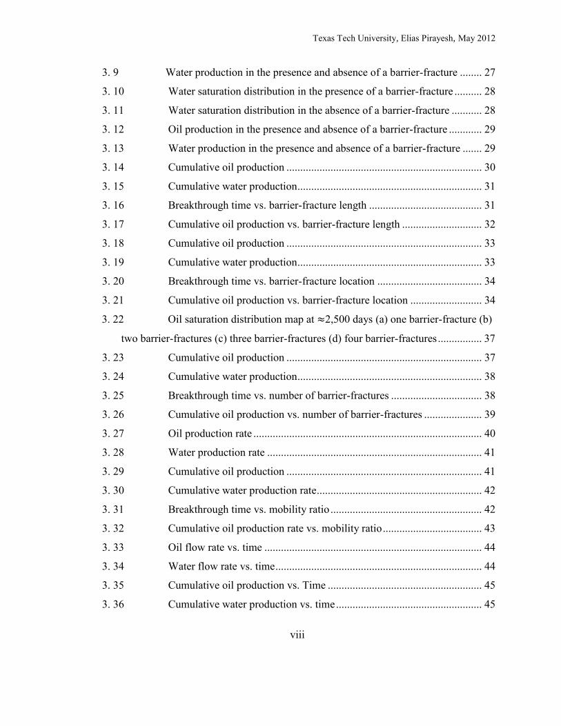
3. 9 Water production in the presence and absence of a barrier-fracture ........ 27

3. 10 Water saturation distribution in the presence of a barrier-fracture .......... 28

3. 11 Water saturation distribution in the absence of a barrier-fracture ........... 28

3. 12 Oil production in the presence and absence of a barrier-fracture ............ 29

3. 13 Water production in the presence and absence of a barrier-fracture ....... 29

3. 14 Cumulative oil production ....................................................................... 30

3. 15 Cumulative water production ................................................................... 31

3. 16 Breakthrough time vs. barrier-fracture length ......................................... 31

3. 17 Cumulative oil production vs. barrier-fracture length ............................. 32



3. 20 Breakthrough time vs. barrier-fracture location ...................................... 34

3. 21 Cumulative oil production vs. barrier-fracture location .......................... 34

3. 22 Oil saturation distribution map at 2,500 days (a) one barrier-fracture (b)

two barrier-fractures (c) three barrier-fractures (d) four barrier-fractures ................ 37



3. 25 Breakthrough time vs. number of barrier-fractures ................................. 38

3. 26 Cumulative oil production vs. number of barrier-fractures ..................... 39

3. 27 Oil production rate ................................................................................... 40

3. 28 Water production rate .............................................................................. 41


3. 30 Cumulative water production rate ............................................................ 42

3. 31 Breakthrough time vs. mobility ratio ....................................................... 42

3. 32 Cumulative oil production rate vs. mobility ratio .................................... 43

3. 33 Oil flow rate vs. time ............................................................................... 44

3. 34 Water flow rate vs. time ........................................................................... 44

3. 35 Cumulative oil production vs. Time ........................................................ 45

3. 36 Cumulative water production vs. time ..................................................... 45


ix

3. 37 Breakthrough time vs. barrier-fracturing time ......................................... 46

3. 38 Cumulative oil production vs. Barrier-fracturing time ............................ 46

3. 39 Cumulative oil production vs. RPM properties ....................................... 47

3.40 Water saturation distribution maps at 1500 days (a) RPM barrier (b)

Barrier-fracture ......................................................................................................... 48

A. 1 Cumulative oil production at 6,000 days vs. number of grid blocks ........ 53


1

CHAPTER I

INTRODUCTION

Excessive water production has been a problem in oil industry for many years.

The two main problems excessive water production causes are wastage of energy for

producing an unwanted fluid and also wastage of oil production potential. To solve this

problem, many research projects have been concentrated on developing conformance

control systems (Dalrymple, Creel et al. 1998). In oil producing wells, unwanted fluid

production conversely impacts the productive life of the well. Produced water treatment

costs have become a major concern for many producers. The control of unwanted fluid

production will allow extraction of more hydrocarbons and consequently increase

profitability (Azari and Soliman 1996).

Conformance control refers to any solution designed for enhancing

injection/production profile of a well. While satisfying environmental regulations,

conformance treatments improve recovery as wells as wellbore integrity. Conformance

treatments involve mechanical or chemical approaches to control the unwanted water or

gas production. These treatments are performed on the producing well, the injection well

or both of them. The treatments may involve minimizing or eliminating the unwanted

fluid production (Azari and Soliman 1996). The first approach, mechanical control, may

involve use of packers or inflow control devices. The second approach, chemical control,

can be divided into several broad groups. The first one involves the injection of a sealant

that is injected into the reservoir to fully stop unwanted fluid flow. The other chemical

approach involves injection of Relative Permeability Modifying (RPM) polymers to

significantly reduce the permeability to water while keeping the relative permeability to

oil fairly intact. Different chemical conformance control methodologies are designed to

reach different effects in the reservoir. An important goal, in most chemical treatments, is

to reduce water relative permeability in the reservoir.

Conformance treatments involve approaches to control the unwanted gas

production as well as unwanted water production. An example of this type is a work done


2

in Prudhoe Bay Field of Alaska. Sanders et al. (1994) showed that cross-linked gels can

be used to shut-off unwanted gas production in a more economical manner compared to

cement squeezes. They also found that gel treatments can successfully block fluid

production from channels behind casing and from several zones with different

permeabilities.

Conformance treatments designed for heterogeneous reservoirs include a wide

variety of methodologies. Among all the existing methodologies, crosslinked-polymers

have gained wide acceptance by the operators; however, there are several critical

problems and limitations related to this technology which include being environmentally

hazardous, limited penetration depth, precipitation and degradation under harsh reservoir

conditions, loss of injectivity, loss of viscosity caused by shear degradation and difficulty

in controlling in-situ gelation rates (Llave 1994). In heterogeneous reservoirs, volumetric

sweep efficiency is highly affected by variations in permeability. The overall efficiency

of an enhanced oil recovery (EOR) process is a function of volumetric sweep efficiency

and microscopic sweep efficiency. An improvement in either one of these two factors can

translate into substantial improvement of economics of an EOR project (Llave 1994).

Llave et al. (1994) evaluated the possibility of using surfactant/alcohol technology

as an in-depth profile modification tool. In-depth modification of flow profile has the

potential of improving volumetric sweep in highly permeable reservoir zones. In-field

application of their proposed methodology resulted in improvements in

injection/production conditions. Some of these improvements include increased oil

production, reduced water production, improved injection profile and delay of water-

breakthrough.

A commonly employed mechanism by conformance control methods is flow

profile modification. Flow profile modification helps improve efficiency by delaying

water/gas breakthrough and improving sweep efficiency. Historical data confirms

effectiveness of profile modification in sandstone and limestone reservoirs (Liu 1995).


3

Profile modification can be accomplished in a variety of different ways. An example of a

profile modification methodology is as follows.

For chemical profile modification, 1980’s was a transition period from purely

experimental method to a routine procedure. Different chemicals including different

categories of gels were in North American heterogeneous reservoirs for profile

modification. These exercises involved selective injection of the polymer into the water-

thief zones. The polymer, after gelation, diverted injected water flow to the unswept oil-

bearing zones. A number of research projects have focused on the general theories behind

chemical profile modification technology, as well as the features and benefits of different

chemicals. (Avery, Burkholder et al. 1986).

One chemical system may work for an entire field, however chemical profile

modification treatments must be designed for each individual well. In designing such

treatments, all available data is used, as to attain the highest rate of success, the designs

must be as comprehensive as possible (Avery, Gruenenfelder et al. 1987).

A profile modification optimization method should be capable of determining

many parameters, including selection of wells and target layers, chemical agents and

injection parameters. Liu et al (2000) introduced a method to optimize the design of

conformance treatments based on profile modification, in which Fuzzy mathematics and

a table of commonly-used 40 chemical formulas provided the basis for the selection of

candidate wells and chemical agents, respectively. In most cases, production analysis

after treatment showed that the waterflood efficiency is improved, and that the model

predictions match well with the actual production data.

Profile modification based conformance control treatments are fairly flexible in

terms of application schedule and treatment combination. For example, over more than

five decades, China oil fields have experienced a series of three stages which include: 1)

mechanical water plugging 2) chemical water plugging and 3) comprehensive treatment

for profile modification in injector and water control in producer of blocks in oil fields.

According to Liu (1995), “Application of water control and profile modification in more


4

than 20,000 well treatments in oil fields from 1979 to 1993 shows that significant

economic and technical benefits as wells as good production results, such as, the increase

of recoverable reserves and oil production and decrease of water production and so on

have been achieved.”

RPMs were first introduced in the late 1970s and were primarily used for water

conformance. Applications were for water fingering, water coning, early water

breakthrough, and communications with water via high perm streaks. A major benefit of

using RPMs was that they are a non-plugging agent, which reduced the permeability to

water and had little or no effect on the permeability to hydrocarbons. They also were

unaffected by multivalent cations, oxygen, or acids (Weaver 1978). However, the nature

of the polymer used to make the initial RPM fluid allowed only a limited application. The

permeability range in which the RPM fluid would work was 10 md to 750 md, the

polymer itself was shear sensitive, and the upper temperature limit was 250°F.

The chemistry of the initial RPMs has been modified by using different polymers

several times since their introduction to the industry. This has allowed several changes

regarding the application and use of RPMs. In the mid-1990s, RPMs were introduced as a

pre-pad fluid in hydraulic stimulation treatments in areas where breaking into nearby

water zones commonly occurred. The results of this application significantly reduced

post-water production after hydraulic stimulation treatment, and allowed operators to

treat and produce previously bypassed formations (Brocco, Dalrymple et al. 2000; Fry,

Everett et al. 2006; Ortega, Peano et al. 2006).

The current RPMs in use, which were introduced to the industry in 2002, are a

fourth-generation polymer and have a broader permeability range. They are not affected

by shear, have an upper temperature range of 325°F. They have greatly extended the

applications where RPM fluids can be used. Fluids that contain the RPM material have

unique properties that allow them to help minimize water production (Nieves, Fernandez

et al. 2002).


5

Once the RPM material is injected into the formation, it rapidly adheres to the

rock surface, hence limiting the ability of water to flow through the formation. While

leaving little or no impact on oil flow, the RPM material restricts the flow area for water-

based fluids substantially. Because this material begins to work immediately, it not only

helps reduce the flow of water being produced, it also helps reduce the amount of a

water-based fluid entering the formation. Therefore, the RPM fluid not only is a self-

diverting fluid, but it also works as a fluid-loss additive that could result in longer

fracture lengths (Garcia, Soriano et al. 2008).

The problem of excessive water production from oil and gas reservoirs can

sometimes be addressed from the injector or producer. It can also be addressed by re-

completing the well or by delaying with cement or polymer gel treatments. However, for

these methods to become feasible the watered-out layer has to be identified and isolated,

which is not always possible. Examples of this include micro-layered formations and

gravel-packed completed wells. The use of RPM agents is an attractive option in these

cases.

Conformance fracturing, a combination of hydraulic fracturing and water control,

has proven as an effective conformance control technique. Hydraulic fracturing has

become the technology of choice for increasing well productivity. Hydraulic fracturing

owes its wide acceptance to the development of the new class of lightweight proppants.

Because of the reduced settling tendency of the proppants, it has become possible to

create more uniform fractures that provide a far better contact with the formation

compared to the past. The chemistry of relative permeability modifiers has also

undergone a lot of change; the most notable result of which is elongated life of water

control treatments using RPMs(Melo and Aboud 2008).

Melo et al (2008) conducted over 100 conformance fracturing operations in Brazil

to date, using conventional as well as lightweight proppants, and relative permeability

modifiers, to meet the different targets they were deployed for. They made a summary of


6

these treatments (design, logistics, materials, equipment), with obtained results (oil and

water production over time), showing the improvements made over time.

Dalrymple et al (1998) discuss field results from conformance fracturing

treatment. The purpose of their treatment was to inject the relative permeability

modifying agent into the fracture while stimulating the reservoir. The RPMs leaked off

into the fracture helped alleviate water production problem. The after-treatment

production data shows a more than 60% increase in oil production, about 60% reduction

in water production and about 120% increase in gas production. It is noteworthy that

previous fracturing treatments had failed in the same field, due to damaging scale and a

subsequent decline in total fluid production.

1.1. Statement of the Problem

A commonly applied enhanced oil recovery solution for recovery improvement is

water-flooding. This mechanism has proven effective in maintaining bottomhole pressure

of many reservoirs around the world. Globally, it has become a common practice to have

injection wells when developing new fields.

The major problem associated with water-flooding projects is the early water-

breakthrough, the main causes of which are high-permeability layers and unfavorable

mobility ratios. Water breakthrough is the main determinant of the productive life of the

reservoir, meaning that after breakthrough, there is a low chance for extracting

hydrocarbons from unswept portions of the reservoir. Also the operational costs will

increase dramatically due to high producing water-oil ratio caused by early breakthrough.

Water-breakthrough solutions usually involve two steps. First, diagnosing the mechanism

to determine the cause and second, applying remediation techniques. The diagnosis can

be performed by production logging, drilling monitor wells, cement evaluation.

Remediation techniques include an extensive number of methodologies, e.g. injecting

sealants, cement and relative permeability modifiers, side-tracking and finally

abandonment. Water-breakthrough treatments sometimes involve changing the flow


7

profile chemically or mechanically. Using cement, different polymers and inflow control

devices are examples of chemical of flow profile modification methodologies.

Water breakthrough treatments can be costly in some cases. Since they are

commonly applied to the near wellbore area of the producer, they are effective only for

reducing water encroachment temporarily. Also, depending on the distance between the

injection and producing wells and productivity of the reservoir, it might take a very long

time to evaluate the performance of these techniques.

1.2. Objective of the Project

The purpose of this project is to investigate the application of barrier-fracturing

using simulation. Barrier-fracturing is a novel idea to modify flow profile and divert the

displacing fluid by placing a fracture with essentially zero permeability deep into the

reservoir. There are many ways to create a zero permeability fracture, examples of which

include injection of cement or a conformance fluid into the fracture. A conformance fluid

can be initially injected as a low viscosity fluid, maybe as low as 0.5 cp., and after

gelation, can reach up 500,000 cp., which eventually become impermeable to any kind of

fluid flow.

Three basic simulation models were created. These include an edge water drive

reservoir, and two other reservoirs which have two different flooding patterns, a line

drive and a five spot pattern. The effects of different design parameters on the

performance of a barrier-fracture were analyzed. These design parameters are listed

below:

1. Barrier-fracture length

2. Barrier-fracture location

3. The number of barrier-fractures

4. Mobility ratio

5. Barrier-fracturing time


8

To achieve our objectives, this report has been divided into four chapters.

Following chapter I, which is an introduction to the problem, the proposed solution

method and the details of the created simulation models will be discussed in Chapter

II. Simulation results and the interpretation of them are provided in Chapter III.

Finally, the conclusions and recommendations for future work are stated in chapter

IV.


9

CHAPTER II

METHODS

As explained in the chapter I, simulation was used as a tool to investigate the

feasibility of achieving recovery improvements by applying the proposed idea. For

optimization purposes, again simulation was used for analyzing the effect of different

design parameters on the performance of a barrier-fracture. All of the simulation runs in

this work were performed by Halliburton commercial simulation software Quiklook ©

version 4.5.232.817.

Three synthetic cases were created. The idea is that the methodology proposed in

this work, could result in some substantial improvements in recovery of the synthetic

cases. The three simulated cases include the following:

1. An edge water drive reservoir

2. A line drive water flooding pattern

3. A five spot water flooding pattern

The reason for selecting these cases is because they represent the most common

problems and the most popular injection/production patterns in use, in oil industry.

The first case simulates the common problem of excessive water production from an

aquifer, caused by water-coning. The next two cases represent reservoirs with two

common injection/production water-flooding patterns in conjunction with a bottom drive

aquifer.

As simulation was used as the analysis tool in this work, there was a need for a

sensitivity analysis on the effect of number of grid blocks. The analysis is presented in

Appendix A.


10

2.1. First case: Edge Water Drive Reservoir

One of the major problems in reservoirs with strong edge water drive is water

coning. Water coning can cause can cause an early water breakthrough, which ends the

productive life of a reservoir. In order to illustrate this problem, a synthetic case of a

reservoir with an edge water drive was created (Figures 2.1 and 2.2). Simulation runs

were performed, and then a fracture was introduced into the model, as is shown in Figure

2.3. Table 2.1 provides data that has been used to create the model.

Figure 2.1. Edge water drive reservoir grid

Figure 2. 2. Edge water drive reservoir map


11

Figure 2. 3. Edge water drive reservoir map with a barrier-fracture

Boundary Status North No-flow South No-flow East No-flow West Aquifer Top No-flow Bottom No-flow

Reservoir fluid type Black Oil Depth to the top of the formation

4002 ft. Rock compressibility 3.00E-06

1/psi Rock reference pressure 6345 psi Depth of water-oil contact 4800 ft. Bubble point pressure 4275 psi Gas specific gravity 0.60 Oil specific gravity 0.89 Water specific gravity 1.00 Irreducible water saturation 0.37 Residual Oil Saturation 0.10 Critical gas saturation 0.05

Table 2. 1. Edge water synthetic case data


12

2.2. Second Case: Line Drive Water Flooding Pattern

In the second case, a reservoir with a line drive flooding pattern with two wells,

an injector and a producer, was simulated. A third well was drilled and a fracture was

placed in the middle of the reservoir. The fracture was then filled up with a conformance

fluid which is capable of forming a gel impermeable to flow of both oil and water. A map

of the reservoir with a fracture in the middle and a vertical profile of the reservoir are

provided in Figures 2.3 and 2.4, respectively.

Figure 2. 4. Line drive reservoir map


13

Figure 2. 5. Line drive reservoir layers

Table 2. 2. Line drive reservoir boundaries

Boundary Status North No-flow South No-flow East No-flow West Aquifer Top No-flow Bottom No-flow

Table 2. 3. Line drive Synthetic case data

Reservoir fluid type Black oil Gas specific gravity 0.60 Depth to the top of the formation

4002 ft. Oil specific gravity 0.89 Rock compressibility 3.00e-06 1/psi Water specific gravity 1.00 Rock reference pressure 6345 psi Irreducible water saturation 0.37 Depth of water-oil contact 4800 ft. Residual oil saturation 0.10 Bubble point pressure 4275 psi Critical gas saturation 0.05


14

2.3. Third Case: Five Spot Water Flooding Pattern

The third case is a reservoir with a quarter of a five spot injection/production

pattern. Like the previous case, there are three wells in the reservoir which include an

injection, a production and a barrier-fractured well. For symmetry purposes, the fracture

was placed in the center of the reservoir. The reservoir map is shown in Figure 5. This

model is the same as the introduced in section 2.2, except for the well locations.

Figure 2. 6. Five spot reservoir map

2.4. Optimization

Later in the results section, it will be shown that the creation of a barrier-fracture

can increase recovery by as much as 10% or even more. In addition to the basic cases, in

order to optimize barrier-fracture design, a number of models with different barrier-

fracture designs were created and simulated. These runs are concentrated on several basic

design factors, which could have the greatest impact on the performance of a barrier-

fracture. These design parameters include barrier-fracture length & location, the number

of barrier-fractures, mobility ratio and schedule of barrier-fracturing.

2.4.1. Barrier-fracture Length

To investigate the effect of barrier-fracture length on the performance of flooding,

several cases with different lengths were created. The reservoir model properties used are

the same as the five spot pattern reservoir in case 3, except for the barrier-fracture length.


15

Different barrier-fracture lengths ranging from 5% to 95% of the reservoir length were

created and introduced into the model. Figures 2.7 to 2.9 show some of these designs.

Figure 2. 7. Barrier-fracture length equal to 25% of reservoir length



16


2.4.2. Barrier-fracture Location

To investigate the effect of barrier-fracture location, several reservoir models with a same

barrier-fracture, placed at different locations were created. To thoroughly investigate the

effect of barrier-fracture location, fractures were placed at 1/4, 1/3, 1/2, 2/3 and 3/4 of the

reservoir length away from the producer and illustrated in figures.

Figure 2. 10. Barrier-fracture placed at the first quarter of the reservoir


17

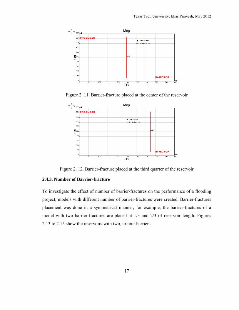
Figure 2. 11. Barrier-fracture placed at the center of the reservoir

Figure 2. 12. Barrier-fracture placed at the third quarter of the reservoir

2.4.3. Number of Barrier-fracture

To investigate the effect of number of barrier-fractures on the performance of a flooding

project, models with different number of barrier-fractures were created. Barrier-fractures

placement was done in a symmetrical manner, for example, the barrier-fractures of a

model with two barrier-fractures are placed at 1/3 and 2/3 of reservoir length. Figures

2.13 to 2.15 show the reservoirs with two, to four barriers.


18

Figure 2. 13. A reservoir with two barrier-fractures

Figure 2. 14. A reservoir with three barrier-fractures

Figure 2. 15. A reservoir with four barrier-fractures


19

2.4.4. Mobility Ratio

In any water-flooding project, mobility ratio is a key determinant of the resulting

recovery of the project. This is because breakthrough time strongly depends on mobility

ratio. In order to analyze the effect of mobility ratio on the performance of a barrier-

fracture, several five-spot pattern reservoirs with different fluid systems were analyzed.

The mobility ratios of these cases range from 0.5 to 10, with 0.5 being a highly favorable

mobility ratio and 10 being a highly unfavorable one.

2.4.5. Schedule of Barrier-Fracturing

The time during the life of a flooding project when the barrier-fracture is created can

affect the performance of a barrier-fracturing project. A barrier-fracture can be created at

any time during a flooding project e.g. before or after water breakthrough. To investigate

the effect that timing has on performance, several models with different barrier-fracturing

times ranging from 0 to 6,000 days were created and simulated. This analysis is important

because in practice, operators have little tendency to start conformance treatments before

breakthrough happens. However the best results are likely to be obtained when the

proposed treatment is applied at the beginning of a flooding project.

2.5. Relative Permeability Modifier Filled Barriers

A selective barrier to flow can be created by injecting a relative permeability

modifying agent (RPM) into a crack created in the reservoir rock. This crack can be a

conventional hydraulic fracture that has not been filled with proppant. Injection of

relative permeability modifying agents into the crack will reduce water relative

permeability to a fraction of its original value while leaving the oil relative permeability

intact. Different relative permeability modifying agents tend to have different effects on

rocks. The range of water relative permeability reduction by injection of relative

permeability modifiers is wide. While leaving oil relative permeability fairly intact, some

RPM agents can cause a 90% reduction in water relative permeability of rocks. This

reduction of water relative permeability will reduce water flow through the treated zone.


20

The effect of relative permeability modifying agents on the relative permeability curves

of a typical rock and a diagram of a barrier created using RPM agents are shown in

Figures 2.16 and 2.17, respectively.

(a)

(b)

Figure 2.16. Reservoir rock relative permeability curves. (a) Before RPM treatment (b) After RPM treatment


21

Figure 2.17. Barrier created by injection of RPM agents into a fracture

Effectiveness of RPM barriers in improving recovery from oil reservoirs was investigated by creating several simulation models. These models are only different in the amount of rock water relative permeability reduction caused as a result of injecting of RPM agents into cracks. The three cases created included RPM barriers with water relative permeabilities ranging from 10% to 75% of the original water relative permeability of reservoir rock.


22

CHAPTER III

RESULTS

The results of the simulations for barrier-fracturing efficiency fall under three

categories as the following:

First case: Edge-water drive reservoir

Second case: A reservoir with a line-drive water-flooding pattern

Third case: A reservoir with a five-spot water-flooding pattern

3.1. First Case: Edge-water Drive

Figures 3.1 and 3.2 show the water saturation distribution in the presence and

absence of a barrier-fracture at 911 days and 914 days, respectively. The comparison of

the saturation profiles in the presence and absence of a barrier-fracture in Figures 3.1 and

3.2 clearly shows the improvement in sweep efficiency by creating the barrier-fracture.

The increase in oil production and decrease in water production are depicted in Figures

3.3 and 4.3. The numerical simulation indicates that the cumulative oil production will

increase by 213,000 STB (5.35%) and decrease in water production will be about the

same amount, 213,000 bbl (6.41%).

Figure 3. 1. Water breakthrough into the horizontal well with no barrier-fracture


23

Figure 3. 2. Water breakthrough into the horizontal well in the presence of a barrier-fracture

Figure 3. 3. Oil production in the presence and absence of a barrier-fracture

0

0.5

1

1.5

2

2.5

3

3.5

4

4.5

0 500 1000 1500 2000 2500 3000 3500 4000

Time, days

To

tal

Oil

Pro

du

cti

on

, M

illi

on

ST

B

With a barrier

Without a barrier


24

Figure 3. 4. Water production in the presence and absence of a barrier-fracture

3.2. Second Case – Line Drive Water Flooding Pattern

Figures 3.5 and 3.6 show the saturation distribution in the presence and absence

of a barrier-fracture. These two figures demonstrate the improved displacement profile

resulting from the creation of the barrier-fracture. Figure 3.7 shows a vertical water

saturation profile in the reservoir. This figure shows how existence of a barrier-fracture

has completely stopped passage of fluids through the fracture. Figures 3.8 and 3.9

illustrate the increase in oil production and decline in water production. The two figures

also indicate that optimization of the fracture position and dimension may be very

important in the design process.

0.00E+00

5.00E-01

1.00E+00

1.50E+00

2.00E+00

2.50E+00

3.00E+00

3.50E+00

0 500 1000 1500 2000 2500 3000 3500 4000

Time, days

To

tal

Wa

ter

Pro

du

cti

on

, M

illi

on

BB

L

With a barrier

Without a barrier


25

Figure 3. 5. Water saturation distribution in the absence of a barrier-fracture

Figure 3. 6. Water saturation distribution in the presence of a barrier-fracture


26

Figure 3. 7. Cross sectional water saturation distribution in the presence of a barrier-fracture



27


3.3. Third Case – Five Spot Water Flooding Pattern

As is illustrated in Figures 3.10 and 3.11, sweep efficiency improves by creating

the barrier-fracture. This is due to the delay in breakthrough caused by the existence of

the barrier-fracture. The increase in oil production and decrease in water production are

shown in Figures 3.12 and 3.13.


28

Figure 3. 10. Water saturation distribution in the presence of a barrier-fracture

Figure 3. 11. Water saturation distribution in the absence of a barrier-fracture


29




30

3.4. Optimization Results

3.4.1. Barrier-Fracture Length

Results of using different barrier-fracture sizes are shown in the following figures.

The cumulative oil and water production are shown in Figures 3.14 and 3.15,

respectively. For this case, the longest fracture produces the best results, i.e. more oil and

less water. Figure 3.16 provides a better relationship between barrier-fracture length and

breakthrough time which is the time when producer oil production rate drop below the

determined production constraint. As expected, the longest barrier-fracture results in the

longest breakthrough time. Figure 3.17 provides a similar relation between recoveries at

6,000 days with different barrier-fracture lengths. Most naturally, the longest fracture

gives the highest recovery among all other fracture lengths.

Figure 3. 14. Cumulative oil production


31

Figure 3. 15. Cumulative water production

Figure 3. 16. Breakthrough time vs. barrier-fracture length


32

Figure 3. 17. Cumulative oil production vs. barrier-fracture length

3.4.2. Barrier-Fracture Location

The results of placing barrier-fractures in different locations in the reservoir are shown in

the following figures. Cumulative oil and water production are shown in Figures 3.18 and

3.19, respectively. These two figures indicate that the barrier-fracture located at the

center of the reservoir would produce the highest amount of oil and the least amount of

water. Figure 3.20 shows how breakthrough time changes as a function of barrier-

fracture location. The barrier-fracture located at 220 ft. away from the producer shows

the longest breakthrough time. Figure 3.21 provides a similar relation between recoveries

at 6,000 days with different barrier-fracture location. Unlike breakthrough time, the

barrier-fracture located at the center of the reservoir gives the highest oil production all

others.

Based on the figures provided, performance of a barrier-fracture is not very sensitive to

barrier-fracture location after all.


33




34

Figure 3. 20. Breakthrough time vs. barrier-fracture location

Figure 3. 21. Cumulative oil production vs. barrier-fracture location


35

3.4.3. Number of Barrier-fractures

Oil saturation distribution maps of all cases at 2,500 days 20 days is shown in Figures

3.22 to 3. Cumulative oil and water production are shown in Figures 3.22 and 3.23,

respectively. A reservoir with four barrier-fractures has produced less water and more oil

over the production period. Figure 3.24 shows breakthrough time changes vs. number of

barrier-fractures. A single barrier-fracture yields the longest breakthrough time. Figure

3.25, provides a similar relationship between recovery and the number of barrier-

fractures. As expected, the design that includes four barrier-fractures results in the highest

recovery.

According to the results of this analysis, a direct relationship between breakthrough time

and the final recovery does not exist with regard to the number of fractures. It is

interesting to see that the improvement in recovery changes only slightly as the number

of barriers is increased from 3 to 4. In a real application, it might not suffice to pay off

the investment made on adding the fourth fracture.

(a)


36

(b)

(c)


37

(d)

Figure 3. 22. Oil saturation distribution map at 2,500 days (a) one barrier-fracture (b) two barrier-fractures (c) three barrier-fractures (d) four barrier-fractures



38


Figure 3. 25. Breakthrough time vs. number of barrier-fractures


39

Figure 3. 26. Cumulative oil production vs. number of barrier-fractures

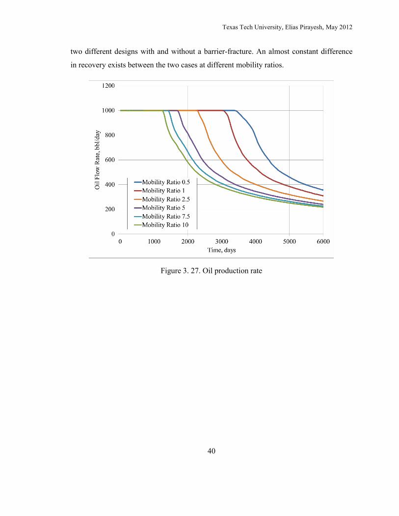
3.4.4. Effect of Mobility Ratio

Results of using different mobility ratios are shown in the following figures. Figures 3.26

and 3.27 show changes in oil and water production rate with time, respectively. Like all

other flooding schemes, cases with lower mobility ratios are expected to produce more

favorable results than those with higher ones. As expected, the case with a mobility ratio

of 0.5 shows a much longer sustained oil flow rate compared to others. It has also

maintained a lower water production rate for the entire production time period. Based on

the figures shown here, it can be concluded that the performance of a barrier-fracturing

project is highly dependent on mobility ratio.

Cumulative production figures (Figures 3.28 and 3.29) confirm the previously obtained

results. Figure 3.30 shows how breakthrough time changes as a function of mobility ratio.

The mobility ratio of 0.5 shows the longest breakthrough time. Figure 3.31 provides a

similar relationship between recovery and mobility ratio. In addition to showing the

effect of mobility ratio, Figures 3.30 and 3.31 can also be interpreted as a comparison of


40

two different designs with and without a barrier-fracture. An almost constant difference

in recovery exists between the two cases at different mobility ratios.

Figure 3. 27. Oil production rate


41

Figure 3. 28. Water production rate



42

Figure 3. 30. Cumulative water production rate

Figure 3. 31. Breakthrough time vs. mobility ratio


43

Figure 3. 32. Cumulative oil production rate vs. mobility ratio

3.4.5. Effect of Barrier-Fracturing Time

Creating a barrier-fracture at different times during the life of a flooding project results in

different production behaviors. Oil and water flow rate vs. time plots are shown in

Figures 3.32, 3.33, 3.34 and 3.35, respectively. Among all the investigated cases, the case

where a barrier-fracture was created at the beginning of the project maintains a higher oil

flow rate and less water flow rate for most of the flooding project. Figures 3.36 and 3.37.

provide a relationship between barrier-fracturing time with breakthrough time and

cumulative oil production at 6,000 days.


44

Figure 3. 33. Oil flow rate vs. time

Figure 3. 34. Water flow rate vs. time


45

Figure 3. 35. Cumulative oil production vs. Time

Figure 3. 36. Cumulative water production vs. time


46

Figure 3. 37. Breakthrough time vs. barrier-fracturing time

Figure 3. 38. Cumulative oil production vs. Barrier-fracturing time


47

3.5. Relative Permeability Modifier Barrier

Based on cumulative oil production results presented in Figure 3.39, RPM barriers have the potential of improving recovery in a water-flooding project; however the amount of improvement in recovery is only marginal. The amount of improvement in recovery also depends on the effectiveness of RPM agents in reducing water relative permeability in rock.

The highest improvement in recovery as a result of creating a RPM barrier is 0.35% where water relative permeability in the barrier was reduced to 10% of its original value. This amount of improvement in recovery is fairly small, especially compared to the improvement achieved by creating a barrier-fracture.

Figure 3. 39. Cumulative oil production vs. RPM properties

The small improvement in recovery achieved by RPM barriers can be explained by analyzing hydrocarbon sweep profiles. In contrast to barrier-fractures, RPM barriers are not effective in changing the sweep patterns in the reservoir. As such RPM barriers cannot change the water paths in the reservoir. Consequently they have very little effect


48

on improving recovery. A comparison between the sweep patterns in the presence of a RPM barrier and a barrier-fracture is presented in Figure 3.40.

(a)

(b) Figure 3.40. Water saturation distribution maps at 1500 days (a) RPM barrier (b)

Barrier-fracture


49

CHAPTER IV

CONCLUSIONS AND RECOMMENDATIONS

The purpose of this project was to investigate the application of barrier-fracturing

using simulation. Barrier-fracturing is a novel idea to modify flow profile and divert the

displacing fluid by placing a fracture with essentially zero permeability deep into the

reservoir.

This research provides three basic simulation models. These include an edge

water drive reservoir, and two other reservoirs which have two different flooding

patterns: a line drive and a five spot pattern. The effects of different design parameters on

the performance of a barrier-fracture were analyzed.

4.1. Conclusions

Based on the saturation distribution maps of reservoirs with and without a barrier-

fracture, a barrier-fracture has the ability to modify flow profile and divert the

displacing fluid.

Barrier-fractures can help improve recovery by delaying water-breakthrough and

improving the volumetric sweep efficiency of a water-flooding project.

Oil production increased and water production decreased as a result of

introducing a barrier-fracture into a reservoir which was under water-flooding.

Barrier-fracture performance can be improved by optimizing design parameters

such as: fracture length, location, number of barrier-fractures, schedule of barrier-

fracturing, and the mobility ratio.

Models with longer barrier-fractures show better performance than those with

shorter barrier-fractures.

The optimum location to place a barrier-fracture is the middle of the distance

between the producer and the injector. Similarly, when there is more than one

barrier-fracture, a symmetrical design with equal fracture spacing is likely to give

the best results.


50

The higher the frequency of barrier-fractures, the higher the performance of

barrier-fracturing. For more than three fractures, the improvement in recovery will

be small, making the economic justification of adding a fracture difficult.

Models with low mobility ratios tend to produce better results than those with

higher mobility ratios, i.e. they show longer breakthrough times, larger

cumulative oil production and less cumulative water production.

Simulation results show that the earlier the barrier-fracture is created, the higher

the recovery will be.

The application of barrier-fracturing is not limited to a specific reservoir type or

completion. It may be applied to a wide variety of conditions such as edge water

drive and various patterns of injection.

RPM-barriers can be created by injecting relative permeability modifying agents

into created cracks in reservoir rock. RPM-barriers are not effective in changing

water flow profile in the reservoir. Consequently, they do not contribute to

recovering more oil from reservoir in a flooding project.

4.2. Recommendations

Streamline simulation provides a convenient tool to investigate enhanced oil

recovery schemes, as it offers a more understandable visualization tool and a

shorter run time. Therefore, it is strongly recommended to use this type of

simulation for comparison of results with those obtained in this work.

Barrier-fracturing needs to be tested with many more types of reservoirs and more

enhanced oil recovery processes such as CO2 injection schemes.

Experimental work can help get more insight into the idea of barrier-fracturing.

For instance, micro-model experiments may provide an easy and reliable tool to

visualize the process.

After experimental investigations, field testing can be the next step in evaluating

the idea of barrier-fracturing.


51

REFERENCES

Avery, M. R., L. A. Burkholder, et al. (1986). Use of Crosslinked Xanthan Gels in Actual Profile Modification Field Projects. International Meeting on Petroleum Engineering. Beijing, China, 1986 Copyright 1986, Society of Petroleum Engineers.

Avery, M. R., M. A. Gruenenfelder, et al. (1987). Design Factors and Their Influence on Profile Modification Treatments for Waterfloods. Middle East Oil Show. Bahrain, 1987 Copyright 1987, Society of Petroleum Engineers.

Azari, M. and M. Soliman (1996). Review of Reservoir Engineering Aspects of Conformance Control Technology. Permian Basin Oil and Gas Recovery Conference. Midland, Texas, 1996,. Society of Petroleum Engineers Inc.

Brocco, C., E. D. Dalrymple, et al. (2000). Relative Permeability Modifier Preflush Fracture-Stimulation Technique Results in Successful Completion of Previously Bypassed Intervals. SPE/DOE Improved Oil Recovery Symposium. Tulsa, Oklahoma, Copyright 2000, Society of Petroleum Engineers Inc.

Dalrymple, E. D., P. Creel, et al. (1998). Results of Using a Relative-Permeability Modifier with a Fracture-Stimulation Treatment. SPE Annual Technical Conference and Exhibition. New Orleans, Louisiana, 1998 Copyright 1998, Society of Petroleum Engineers Inc.

Fry, L. E., D. M. Everett, et al. (2006). Successful Application of Relative-Permeability Modifiers To Control Water Production in Rose Run Fracturing. SPE Eastern Regional Meeting. Canton, Ohio, USA, Society of Petroleum Engineers.

Garcia, B., J. E. Soriano, et al. (2008). Novel Acid-Diversion Technique Increases Production in the Cantarell Field, Offshore Mexico. SPE International Symposium and Exhibition on Formation Damage Control. Lafayette, Louisiana, USA, Society of Petroleum Engineers.

Liu, X.-E. (1995). Development and Application of the Water Control and Profile Modification Technology in China Oil Fields. International Meeting on Petroleum Engineering. Beijing, China, 1995 Copyright 1995, Society of Petroleum Engineers, Inc.

Llave, F. M. (1994). Field Application of Surfactant-Alcohol Blends for Conformance Control. SPE Annual Technical Conference and Exhibition. New Orleans, Louisiana, Society of Petroleum Engineers.

Melo, R. C. B. D. and R. S. Aboud (2008). Over 100 Conformance Fracturing Operations in Brazil: Results and Improvements. Europec/EAGE Conference and Exhibition. Rome, Italy, Society of Petroleum Engineers.


52

Nieves, G., J. Fernandez, et al. (2002). Field Application of Relative Permeability Modifier in Venezuela. SPE/DOE Improved Oil Recovery Symposium. Tulsa, Oklahoma, Copyright 2002, Society of Petroleum Engineers Inc.

Ortega, A. T., J. R. Peano, et al. (2006). Conformance While Fracturing: Technology Used To Reduce Water Production in North Mexico. First International Oil Conference and Exhibition in Mexico. Cancun, Mexico, Society of Petroleum Engineers.

Weaver, J. D. (1978). A New Water-Oil Ratio Improvement Material. SPE Annual Fall Technical Conference and Exhibition. Houston, Texas, 1978 Copyright 1978, American Institute of Mining, Metallurgical, and Petroleum Engineers, Inc.


53

APPENDIX A

SENSITIVITY ANALYSIS: EFFECT OF GRIDDING ON SIMULATION

RESULTS

Using simulation as the analysis tool in this work necessitates a sensitivity analysis to ensure that the reported results are not affected by the number of grid blocks used in simulation models. In this study, the most commonly used simulation model is the case of a reservoir with a five spot flooding pattern. The reservoir grid is a 42 41 13 system. Cumulative oil production at 6,000 days vs. total number of grids is shown in Figure A.1.

Figure A. 1. Cumulative oil production at 6,000 days vs. number of grid blocks

The plot shows that increasing the number of grid blocks from 16,380 (36 35 13) to 123,578 (98 97 13) will cause a difference of 0.6% in cumulative oil production at 6,000 days. This shows that the simulation results are relatively insensitive to the number of grid blocks and any grid system between 36 35 13 and 98 97 13 can be an optimal gridding candidate.


54

VITA

Permanent Address:

Bob L. Herd Department of Petroleum Engineering Texas Tech University, Lubbock TX 79409

Email Address:

[email protected]

Education:

M.Sc., Petroleum Engineering

Texas Tech University

Lubbock TX 79409 B.Sc., Petroleum Engineering

Sharif University of Technology

Tehran, Iran

mailto:[email protected]

Improving Volumetric Sweep Efficiency in Enhanced Oil ...

Documents

Transcript of Improving Volumetric Sweep Efficiency in Enhanced Oil ...