Self-Improving Reactive Agents Based On Reinforcement Learning, Planning and Teaching

IMPROVING THE SURVIVABILITY OF AGENTS IN A FIRST-
PERSON SHOOTER URBAN COMBAT SIMULATION BY
INCORPORATING MILITARY SKILLS
By,
Ashish C. Singh
A thesis submitted in partial fulfillment of
the requirements for the degree of
MASTER OF SCIENCE IN COMPUTER SCIENCE
WASHINGTON STATE UNIVERSITY
School of Electrical Engineering and Computer Science
DECEMBER 2007

ii
To the Faculty of Washington State University:
The members of the Committee appointed to examine the thesis of
ASHISH C. SINGH find it satisfactory and recommend that it be accepted.
___________________________________
Chair
___________________________________
___________________________________

iii
ACKNOWLEDGEMENT
I would like to thank my advisor, Dr. Holder, for his guidance and support. I would also like to
thank Dr. Cook and Mr. Hagemeister for their valuable advice while serving on the committee.
And I would like to thank Nikhil Ketkar and my family for their valuable guidance.

iv
IMPROVING THE SURVIVABILITY OF AGENTS IN A FIRST-PERSON SHOOTER
URBAN COMBAT SIMULATION BY INCORPORATING MILITARY SKILLS
Abstract
by Ashish Singh, M.S.
Washington State University
December 2007
Chair: Dr. Lawrence Holder
The exhibition of intelligence while selecting paths in a combat setting should be based
upon the right balance of the risk involved and the traversal time. In this work we propose an
algorithm that finds strategic paths inside an urban combat game map with a set of enemies. The
strategic path calculation is based upon the hit probability calculated for each enemy’s weapons
and the risk vs. time preference. Ultimately, the strategic path calculation minimizes both time
and risk as per mission objectives. The strategic path planning concept can be applied to both
Real Time Strategy (RTS) and First Person Shooter (FPS) games.
We propose evaluating a map at two levels of abstraction: Area level and Grid level. Area
level strategic path computation can be done at run-time, because Areas are far less in count
compared to Waypoints. When the agent reaches the computed Area, the strategic path is
computed over the Grid Points of that Area. Thus, the calculation of the hit probability can take
into account the real-time movements of the enemies as the agent traverses the Grid Points of an
Area.
Secondly, in addition to the computational savings of calculating strategic paths at the
Area level, rather than the Grid level (or using Waypoints), there is also the issue of not knowing
visibility details within an Area until the agent arrives at that Area, especially in urban combat
settings. Thus the agent exhibits intelligence (in strategic path computation) in a more realistic
way.

v
We performed out-game and in-game experiments on our proposed model of strategic
path computation and found that the computed strategic paths based upon a high risk vs. time
preference are significantly safer.

vi
TABLE OF CONTENTS
Page
ACKNOWLEDGEMENTS .................................................................................................iii
ABSTRACT ......................................................................................................................... iv
LIST OF TABLES ............................................................................................................... vi
LIST OF FIGURES ............................................................................................................ vii
CHAPTER
1. INTRODUCTION ................................................................................................. 1
2. RELATED WORK ................................................................................................ 3
3. THE TESTBED ENVIRONMENT ....................................................................... 7
4. VISIBILITY AND 3D VOLUME SEARCH ALGORITHM ............................. 14
5. STRATEGIC PATH PLANNING AT AREA LEVEL ....................................... 20
6. GRID PATH PLANNING AT GRID LEVEL .................................................... 32
7. EXPERIMENTATION AND VALIDATION .................................................... 39
8. OTHER APPLICATIONS OF STRATEGIC PATH PLANNING .................... 52
9. CONCLUSION AND FUTURE WORK ............................................................ 58
BIBLIOGRAPHY ............................................................................................................... 62
APPENDIX

vii
LIST OF FIGURES
Page
1. Quake3 Arena ........................................................................................................... 2
2. The UCT HUD .......................................................................................................... 8
3. Top view of the Reykjavik map ................................................................................ 9
4. Formalizing into set of Areas and Gateways .......................................................... 10
5. The agent’s interface ............................................................................................... 11
6. Double use of polygonal areas ................................................................................ 15
7. A portion of the map converted to a graph ............................................................. 22
8. Strategic Distance is a trade-off between Risk and Time ....................................... 24
9. In Strategic path computation tactical distance from a more dangerous enemy is
maximized ............................................................................................................... 25
10. Hit probability based upon range modeled for three weapons ............................... 26
11. Checkpoint distribution along a pair of areas. ........................................................ 28
12. For path traced the checkpoint count can be less .................................................... 30
13. The strategic path at Area level for Area-105 ......................................................... 31
14. The strategic path at Grid level for Area-105 ......................................................... 37
15. Strategic Path completely avoided the enemy ........................................................ 47
16. Plots of variations in Avg. Output Hit Probabilities with different weapons ......... 48
17. Plots of Hit Probabilities for one enemy situation with RISK_VS_TIME = 10 ..... 49
18. HP variation between Meta-Weight computation and Path’s risk evaluation for 1m
checkpoint ............................................................................................................... 51
19. HP variation between Meta-Weight computation and Path’s risk evaluation for 0.5
checkpoint ............................................................................................................... 52
20. Avg. distance of shortest paths, strategic paths over Area and Grid level .............. 53
viii
21. In-Game trial experiment results for RiskVsTime=5 ............................................. 54
22. In-Game trial experiment results for RiskVsTime=10 ........................................... 56
23. The average hit probability for the in-game trials .................................................. 57
24. The average time of successful walks on strategic and grid paths ......................... 59
25. Strafing and shooting .............................................................................................. 60
26. Safely reached experiment count analysis of agent with shooting skills ................ 61
27. Safely reached average time analysis of agent with shooting skills ....................... 62
28. Safely reached experiment count analysis of agent without shooting skills ........... 63
29. Safely reached average time analysis of agent without shooting skills .................. 64
30. Strafe, aim, shoot and take cover ............................................................................ 65
31. Basic Strategic tactics ............................................................................................. 68
32. Shoot and Scoot tactics ........................................................................................... 69
33. Ambush MOUT strategy......................................................................................... 71

ix
LIST OF TABLES
Page
1. Algorithm: LOS algorithm ...................................................................................... 18
2. Algorithm: 3D volume search algorithm ................................................................ 19
3. Algorithm: Strategic Path Planning at Area level Algorithm ................................. 34
4. Algorithm: Grid Point computation on the Gateways ............................................ 38
5. Algorithm: Grid Point computation inside an Area ................................................ 40
6. Algorithm: Basic Strategic tactics .......................................................................... 68
7. Algorithm: Shoot and Scoot MOUT tactics: .......................................................... 69
8. Algorithm: Ambush MOUT tactics ........................................................................ 72

1
CHAPTER ONE
INTRODUCTION
In a combat scenario where there are enemies, the shortest path towards the goal is not
always the best path, especially when it is well guarded. Thus, if an agent follows an unknown
path that has been considered as the best path and in this path an enemy spots the agent and
shoots him, the goal remains unachieved. Instead depending upon the mission objective if the
agent can afford to take a safer path that takes advantage of areas hidden from the enemy to
provide cover, then the agent can achieve the goal and maintain good health. This type of path
planning is useful for Military Operations on Urban Terrain (MOUT) tactics. We have developed
a strategic path planning algorithm that is based upon in-depth risk evaluations along all the
possible paths that can lead to the goal. For that we use the Hit probability for calculating the risk
involved on a path. The risk calculation takes into account all the enemies.
We also propose a 3D volume organization technique which we call the Heuristic Search
Space (HSS) technique (discussed in a later chapter). For the visibility calculation we propose a
Brush Collision Detection algorithm (discussed in [14] and that has been used with Binary Space
Partition (BSP) trees in Quake3 [18]) to be used with our HSS technique. We implement and test
the strategic path computational model using these techniques in the context of a MOUT
scenario within the Quake3 first-person shooter computer and video game.
Quake 3 Arena is a multiplayer FPS game released on December 2, 1999 [24]. The game
was developed by id Software. In Quake3, a player collects points (called frags) by killing other
players. Quake3 Arena features Deathmatch, Team Deathmatch, Capture the flag, and
tournament, in which players test their skills against each other in one-on-one battles and an
elimination ladder [24]. See Figure 1 for a snapshot from the game. On August 19, 2005, id

2
Software released the complete source code for Quake III Arena under the GNU General Public
License [24].
Figure 1: Quake3 Arena
We performed an empirical analysis of our strategic path computational model based on
our MOUT modification of the Quake3 game. In our experiments we defined 50 random
experiment sets. Each experiment set has a defined RiskVsTime factor, agent’s start location,
agent’s goal location and enemy’s location. For each of 50 experiments we evaluated all three
paths, Shortest Path, Strategic Path at Area level and Strategic Path at Grid level, using both out-
game and in-game trials.
In out-game trials we used the real world weapon details [5] to compute the hit
probability (HP) across the traced path between the start and the goal location.

3
We used the Urban Combat Testbed (UCT) for our in-game trials. The UCT is an Urban
Environment based modification of Quake3. The agent program interacts with the UCT using
shared memory access. Here, the hit probability for each experiment is computed by computing
the average hit probability over 10 runs.
On experimentation, we found the paths generated by the strategic path computation were
safer (the difference between the risks was statistically significant) with a trade-off of longer
distance to walk. In out-game trials, we found the Strategic path Grid level performed
consistently better than the Strategic path at Area level by further reducing the distance of walk.
In chapter 2, we have compared our work with the research work done in this field.
Chapter 3 discusses our Testbed environment and addresses how an agent interacts with the
Testbed environment. In chapter 4, visibility algorithms have been discussed. Chapter 5
describes the conceptual definition of risk that we address in our work. It also discusses our
algorithm for strategic path computation at Area level. Chapter 6 discusses our algorithm for
strategic path computation at Grid level and explains how the strategic path computation at Grid
level is connected to strategic path computation at Area level. Chapter 7 discusses our out-game
and in-game trial setup. Chapter 8 contains our experimental results. Chapter 9 discusses MOUT
strategies and tactics that can be implemented using this work. And chapter 10 contains the
conclusion and also addresses the possible enhancements and the significance of this work to
Real Time Strategy (RTS) games.

4
CHAPTER TWO
RELATED WORK
2.0 Overview
This chapter discusses how the simple path planning problems are related to the strategic
path computation. This chapter also discusses previous work done in this field, compares our
work and discusses our contribution.
2.1 The Shortest Path
Path planning and collision prevention for single and multiple players has been
extensively studied [6]. But strategic path planning is a relatively new area of study. Shortest
path planning can be done on waypoints by applying the A* algorithm [10]. But this approach
neglects the strategic importance of waypoints.
2.2 Previous work
Various strategies and tactics for Military Operations on Urban Terrain (MOUT) depend
upon the visibility among waypoints. In this direction by using the BitStrings technique [1] used
by Liden for strategic path planning to exhibit a potential for MOUT tactics like flanking [1].
BitStrings decreases computation and storage requirements for visibility computation at run-
time. In the BitStrings technique a bit represents visibility information between two waypoints.
Each waypoint maintains a Bit String that contains visibility information of all the waypoints
from that waypoint (in form of true or false). Therefore computation about the visibility from an
enemy’s waypoint does not need to be computed at run-time.

5
In their work risk has not been studied in detail. Risk is defined by the ability of an enemy to kill
the agent. It makes the following assumptions.
(I) A far distant enemy has been considered equally risky compared to short distant enemy.
(II) A variation in fire power of an enemy has not been considered. For example Sniper and
Sub-Machine Gun have not been considered separately.
(III) BitStrings can only be used for a fixed set of waypoints. In real 3D environments, the
visibility complexity increases and the set of fixed waypoints cannot address strategic
importance of visibility accurately.
2.3 Our contribution
We extend this work to find a strategic path with the help of weight and path matrices
and also prioritize these paths on the basis of a risk vs. time factor. Instead of using a large
number of waypoints we have abstracted it to a smaller number of polyhedron areas [3] and
inside these areas we calculate visibility by using a checkpoint approach discussed in chapter 5.
We also present an efficient Line of Sight (LOS) algorithm that can be significantly optimized by
using the Heuristic Space Search technique. We also conducted various tests on a realistic
MOUT based environment with the real visibility computational challenges.
Our work features,
(I) We compute the risk from the realistic hit probabilities [5] computed for all the
enemies based upon the distance from the enemies. Thus, our risk calculation
addresses all the components of risks (type of weapon and its lethality).
(II) First, the strategic path is computed over the set of Areas (an abstraction of walk-
able areas). They are far less in count compared to Waypoints. Thus the risk

6
computation can be done at run-time and it takes into account all the dynamic
changes.
(III) Secondly, while walking over the selected Areas the strategic path is computed at
Grid level (the Grid level, a higher level of detail). This computation gives the
within-area Grid Points to walk through after reaching a selected area. Thus, the
calculation of the hit probability can take into account the real-time movements of
the enemies as the agent traverses the Grid Points of an Area.
(IV) Thus, by doing the strategic path computation at two levels the computational
burden gets linearly distributed. As Grid level can go into a more detail than the
fixed set of Waypoints and therefore it covers more strategically significant
locations.
(V) Secondly, in addition to the computational savings of calculating strategic paths at
the Area level, rather than the Grid level (or using Waypoints), there is also the
issue of not knowing visibility details within an Area until the agent arrives at that
Area, especially in urban combat settings. Thus the agent exhibits intelligence (in
strategic path computation) in a more realistic way.
(VI) The Areas can be computed automatically (in Quake3 they are similar in concept
to clusters separated by cluster portals [19]) and further Grid points are also
automatically computed. And on the other hand optimal distribution of Waypoints
does require intervention of level designers [19].

7
CHAPTER THREE
THE TESTBED ENVIRONMENT
3.0 Overview
This chapter discusses our Testbed environment. And later in this chapter agent’s
percepts have been discussed. They are categorized into Static and Dynamic percepts. And later
types of actions the agent can perform have been discussed.
3.1 Urban Combat Testbed
Our experiments were performed on the Urban Combat Testbed (UCT) [3]. UCT is a
modification of the Quake3 [18,19] first person shooter game.
The agent program interacts with the UCT using a shared memory interface exchanging
percepts and actions. The shared memory is used to read and write percepts and actions with
lower communication latency and lower computational burden on the game engine. Figure 2
contains a snapshot of UCT’s heads-up display (HUD).

8
Figure 2: The UCT HUD
The Reykjavik map (figure 3) is a model of an urban area. It contains four small building
structures connected by streets. It also contains other urban features like garage, walls, pallets, a
bus-stop, street-lights, trees, crates. Areas inside this map vary in latitude. The size of the map is
3376 x 2976 x 640 inches (85.75 x 75.59 x 16.25 meters).

9
Figure 3: Top view of the Reykjavik map [20]

10
3.2 Areas and Gateways [3][21]
Figure 4: Formalizing into set of Areas and Gateways
The walkable surfaces in the map have been defined as Areas. In Quake3 Areas are
similar to clusters concept and the gateways are similar to cluster portal concept [19]. These
areas are 3D boxes made up of convex polygons (6 or more). Areas have been constructed from
the 3D brushes used to define a map in Quake3. Figure 4 shows the areas computed for the map
in figure 3. All walkable areas are connected using gateways. Gateways also contain information
about the type of action required to cross the gateway from one area to another area (actions like
Jump, Walk, Fall, etc.).

11
3.2.1 Area and Object Construction [3][21]
All the 3D volumes are classified into positive and negative spaces. A 3D volume like a
wooden-box where an agent cannot walk-in is called as a positive space (called Objects) and on
the other hand an open surface like a ground area where an agent can stand or walk-in has been
classified as a negative space (called Areas). A building by itself is an Object but inside it also
contains floors where an agent can stand, these floors are Areas. Using Quake 3 map editor
(GTKradiant [22]) one has to manually box all the 3D volumes as positive and negative spaces.
And by using the Sarge application [3,21] 3D coordinates and normals of planes boxing all the
3D volumes are computed and recorded into an XML file.
3.2.2 Gateway Construction [3][21]
An Area can be traversed to its neighboring Area by actions like walk, jump, fall or none
between the connections (openings) of the two Areas that will be a polygonal surface (called
Gateway). Using the Sarge application the connection between every two Areas is computed and
recorded into the same XML file.
3.3 The Agent’s interface
Figure 5: The agent’s interface
The percepts are of two types: dynamic and static. As shown in figure 5, the agent
retrieves the Static Percepts from a Static Spatial Perception Service (SSPS) XML file. And it

12
receives Dynamic Percepts from the UCT and after processing the percepts it sends its Actions
back. This communication is done through the shared memory interface (as shared memory has a
very low latency).
3.3.1 The Dynamic Percepts
The dynamic percepts include information about current location (X, Y, Z coordinate
form), yaw, pitch, roll, health, weapons and ammunitions, in other words these percepts are
meant to change with the game play. The dynamic percepts consist of 33 different percepts
related to the player, 11 different percepts about entities which include opponents if they are
present and all the different dynamic objects, and 4 different percepts about weapons.
3.3.2 The Static Percepts
The static percepts contain the map information. The static percepts are the information
about the static entities in the map like walls, areas, objects etc. The static map information is
passed to the agent using an XML description [3][21]. The XML file contains plane coordinates,
normals and a unique ID for all the Areas and Objects. It also contains connectivity information
about those Areas called Gateways and type of action required to traverse from one Area to
another neighbor Area.
3.3.3 The Actions
The agent program can choose from 29 different actions that can be sent to the game. The
actions are of very primitive form (WALK_FORWARD, TURN_RIGHT, TURN_LEFT,
WALK_BACKWARD, RELOAD, FIRE, STRAFE_LEFT, STRAFE_RIGHT etc). These

13
actions are categorized into four categories and written into the assigned shared memory. The
agent program can write together a set of four actions. These four actions can be performed
together. The UCT reads these actions and executes accordingly. Thus, an agent can perform
multiple actions together, e.g., Strafe and Shoot (the agent can move to a safe location while
shooting). Similarly, it can Turn and Walk together making its path smoother.
14
CHAPTER FOUR
VISIBILITY AND 3D VOLUME SEARCH ALGORITHM
4.0 Overview
An Area at a higher height can block visibility between two of its neighboring Areas at
lower heights. Therefore, Areas and Objects both must be considered for visibility computation.
This chapter discusses how the information about an Area retrieved from a SSPS XML file is
used for both visibility and location reasoning (for retrieving Area connectivity). We used
Heuristic Search Space (HSS) technique to get to a small set of probable 3D volumes that could
obstruct the visibility between two points. Then we applied Quake3’s brush collision technique
to determine whether the two points are really blocked by a 3D volume out of all the probable
3D volumes (algorithm 4).
And similarly for searching the 3D volume for a given XYZ point, HSS reduces the
number of 3D volumes to search to a very small list of probable 3D volumes (algorithm 5).
15
4.1 Visibility between Areas
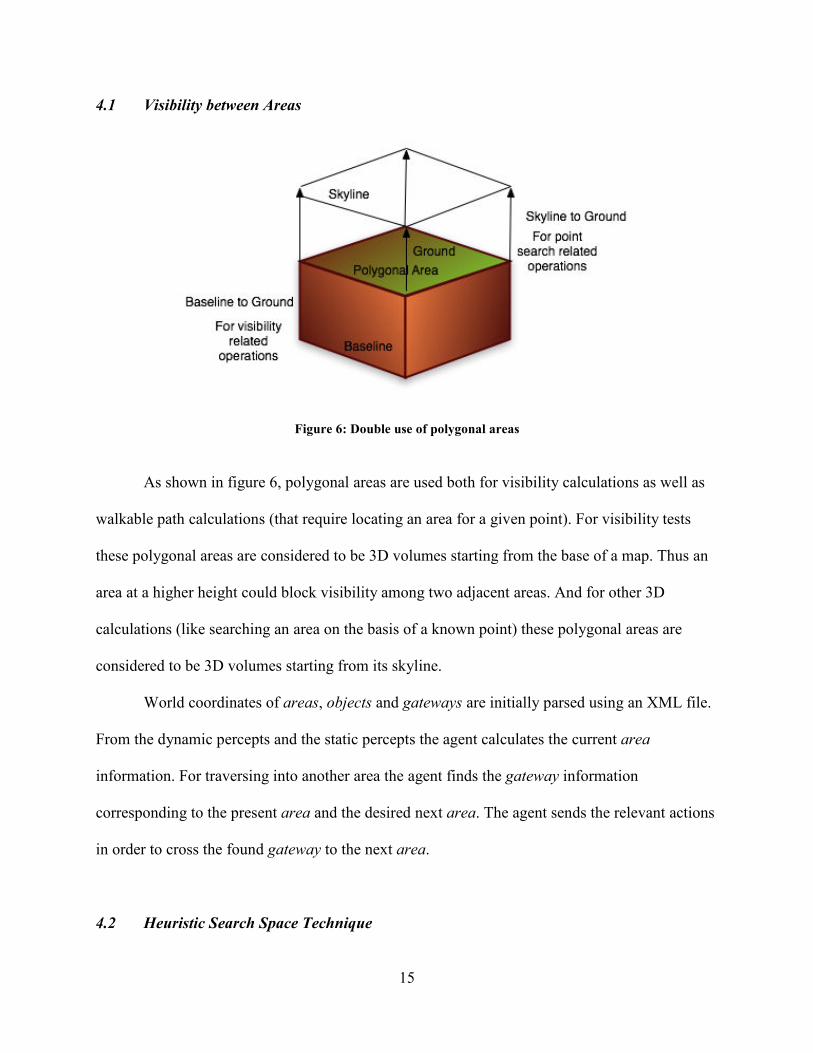
Figure 6: Double use of polygonal areas
As shown in figure 6, polygonal areas are used both for visibility calculations as well as
walkable path calculations (that require locating an area for a given point). For visibility tests
these polygonal areas are considered to be 3D volumes starting from the base of a map. Thus an
area at a higher height could block visibility among two adjacent areas. And for other 3D
calculations (like searching an area on the basis of a known point) these polygonal areas are
considered to be 3D volumes starting from its skyline.
World coordinates of areas, objects and gateways are initially parsed using an XML file.
From the dynamic percepts and the static percepts the agent calculates the current area
information. For traversing into another area the agent finds the gateway information
corresponding to the present area and the desired next area. The agent sends the relevant actions
in order to cross the found gateway to the next area.
4.2 Heuristic Search Space Technique

16
With the help of this technique, we can limit the number of visibility tests to a very small
number of visibility tests and this count is independent of the total 3D volumes. And also this
technique efficiently finds the list of probable 3D volumes occupying a given XYZ location by
searching through the 3D volumes associated with that HSS element instead of the total count of
3D volumes.
4.3 Indexing 3D Volumes
In this technique we index the complete 3D map to a small 3D array. Each element in that
array points to a list of 3D volumes (Areas and Objects) in the corresponding 3D space of the
map. For example when HSS edge length is 100 each 3D space of 100x100x100 will be
associated with one element of the Heuristic Search space (HSS), and it will store the list of
Areas and Objects occupying (may or may not completely) that 3D space. Thus, areas and
objects that could exist inside that 3D space of the map will be addressed by a very small 3D
array. For example a 3D map of size 4000x4000x1000 in the Heuristic Search Space can be
efficiently indexed into a 3D array of size 40x40x10.
To efficiently calculate the set of HSS elements that will store a 3D volume, we just need
to find two extreme points (xmin, ymin,, zmin) and (xmax, ymax,, zmax) of that 3D volume and step
through all the points inside this space in multiples of HSS edge length. These computed points
are listed accordingly with appropriate HSS elements.
4.4 Visibility Test
17
For the visibility test between two points we search between these points for any 3D
volume that could block the visibility. Thus, if a line segment joining these two points gets
intersected by a 3D volume then it will be considered as a visibility blockage (refer Algorithm 1)
We transform the visibility problem in the original map to a visibility problem in HSS.
Since HSS uses a more abstract and a more simple representation of the original map, it produces
a list of probable 3D volumes that could block the visibility between the points of the original
map. For example, in HSS a line segment between points {(1200, 1200, 40), (3000, 2000, 100)}
will be indexed as {(12, 12, 0), (30, 20, 1)}. Thus, in HSS all the 3D objects that are associated
with the line joining these points will be computed for visibility tests. This technique minimizes
the potential 3D objects for visibility tests.
The Binary Search Partition (BSP) technique in the Quake3 engine keeps record of all the
3D brushes even when smaller brushes have no strategic significance. The BSP technique can be
applied directly to SSPS 3D volumes. Whereas, the HSS technique meant for SSPS 3D volumes
will directly reach the potential candidates in a constant time (independent of the total count of
3D volumes inside the map, but it varies with the map’s dimensions). On the other hand the BSP
technique searches through the root node to the potential set of brushes (polyhedral volumes) by
comparing log(n) partition planes where n is total partition planes. For cases where two points
are separated by a small distance the HSS technique will perform better than the BSP technique
because BSP will go through log(n) partition planes and on the other hand HSS will list 3D
volumes that are associated with the HSS elements along the line joining the two points.
But, the HSS technique cannot be a better choice for all the cases. For cases where a 3D
map is poorly indexed the HSS technique will produce a large list of probable 3D volumes. Thus,

18
it will increase the number of visibility tests before reaching the correct 3D volumes for decisive
visibility tests.
Algorithm 1: LOS algorithm
INPUT: Two points, the static percepts and indexed HSS.
OUTPUT: Result of blockage in visibility as true or false.
SYNOPSIS: This algorithm checks visibility between two locations
for strategic path planning. The given two points are mapped to
HSS and the appropriate two HSS locations. And among these two
HSS locations a line is drawn. And all the visited HSS elements are
searched for their associated 3D volumes. These 3D volumes and
the given two locations are the reduced test-cases for the brush
collision algorithm [14] (of Quake3 engine) and on any successful
blockage return true else continue with other listed 3D volumes.
ALGORITHM:
1: Locate HSS element for both the points.
2: Construct a line segment between above two HSS elements
in HSS. And obtain all the HSS elements on that line.
2: For each 3D volume associated with the above HSS elements.
Perform step 3.
3: Input two points and a 3D volume [14].
3.1: Locate sides of the two points for each face of the
3D volume.
3.2: If both the points are outside of any of the face.
Then reject this 3D volume else continue with
other sides.
3.3: If both the points are inside of any of the face.
Then continue to step 3.4.
19
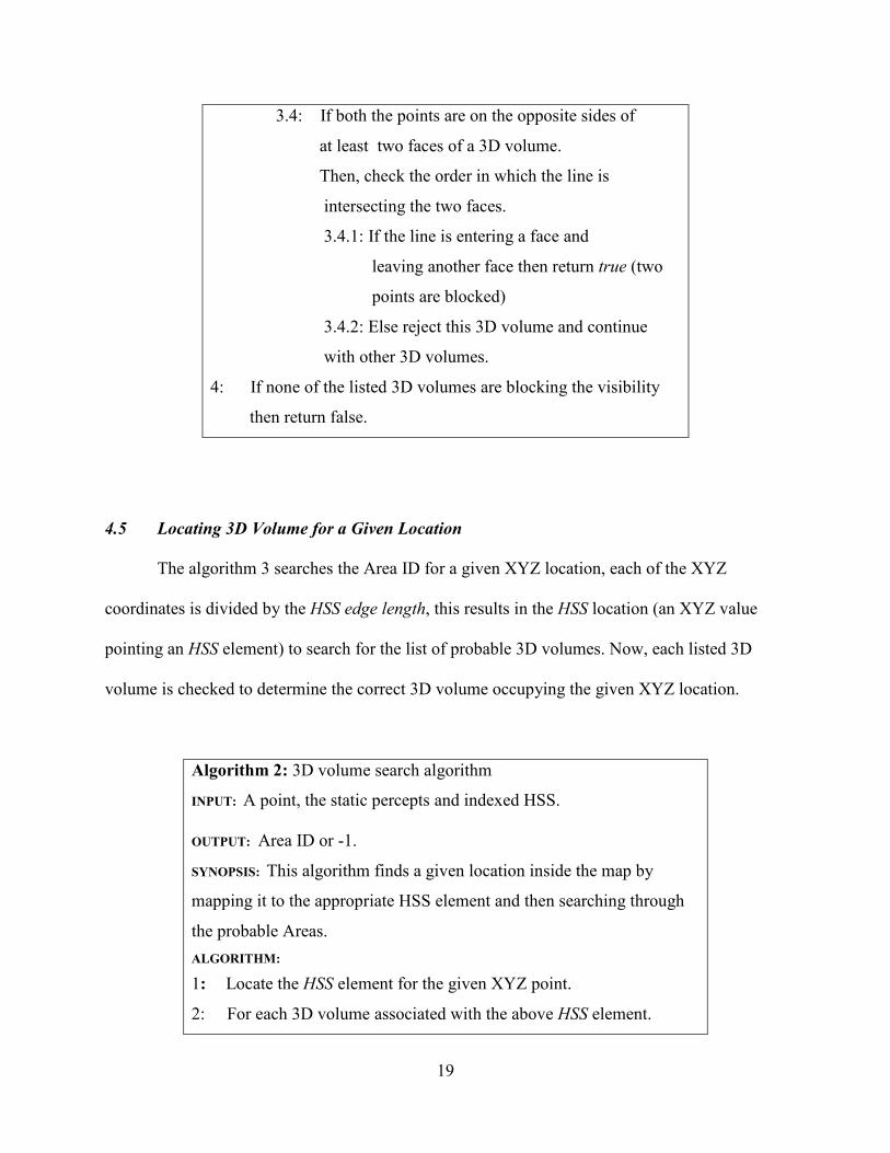
3.4: If both the points are on the opposite sides of
at least two faces of a 3D volume.
Then, check the order in which the line is
intersecting the two faces.
3.4.1: If the line is entering a face and
leaving another face then return true (two
points are blocked)
3.4.2: Else reject this 3D volume and continue
with other 3D volumes.
4: If none of the listed 3D volumes are blocking the visibility
then return false.
4.5 Locating 3D Volume for a Given Location
The algorithm 3 searches the Area ID for a given XYZ location, each of the XYZ
coordinates is divided by the HSS edge length, this results in the HSS location (an XYZ value
pointing an HSS element) to search for the list of probable 3D volumes. Now, each listed 3D
volume is checked to determine the correct 3D volume occupying the given XYZ location.
Algorithm 2: 3D volume search algorithm
INPUT: A point, the static percepts and indexed HSS.
OUTPUT: Area ID or -1.
SYNOPSIS: This algorithm finds a given location inside the map by
mapping it to the appropriate HSS element and then searching through
the probable Areas.
ALGORITHM:
1: Locate the HSS element for the given XYZ point.
2: For each 3D volume associated with the above HSS element.
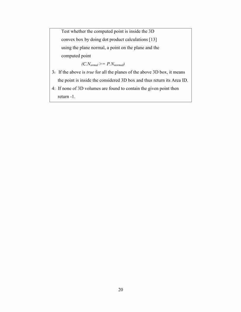
20
Test whether the computed point is inside the 3D
convex box by doing dot product calculations [13]
using the plane normal, a point on the plane and the
computed point
(C.Normal >= P.Nnormal)
3: If the above is true for all the planes of the above 3D box, it means
the point is inside the considered 3D box and thus return its Area ID.
4: If none of 3D volumes are found to contain the given point then
return -1.
21
CHAPTER FIVE
STRATEGIC PATH PLANNING AT AREA LEVEL
5.1 Overview
This chapter discusses the conceptual definition of risk that we address in our work. It
also discusses our Testbed environment and describes our algorithms.
5.2 Definition of Risk
A path that takes the agent to areas closer and visible to an enemy is a risky path. Risk is
defined as the ability to shoot the player in terms of Hit Probability (HP). Each weapon has a
different hit accuracy, rate of fire and hit ratio per bullet fired. We used weapon details [5] to
obtain a hit probability based upon distances from a set of enemies. Each weapon has a different
Hit Probability and the distance between the agent and the enemy is almost inversely
proportional to the hit probability. The enemy’s ability to shoot the agent depends upon three
factors:
(I) The agent’s visibility from the enemy’s location.
(II) The distance from the enemy.
(III) The lethality of the enemy’s weapon.
A strategic path is a trade-off between the time of traversal and the risk along the path. Not
all the areas along all the possible paths are completely covered (no risk along the path because
none of the enemies can see it). Therefore the risk evaluation must carefully consider all of the
three components of risks.
22
5.3 Formalizing Areas and their Connectivity as a Graph
Areas and their connectivity can be formalized as vertices and edges of a graph. Thus,
finding a path among areas becomes a problem of finding a path in a graph. The connectivity
between areas resembles connections between vertices. The Euclidean distances between areas
become weights on the edges (in our case we measured the distance between the area centers
going through the gateway center when “walk” is the action of the gateway between areas).
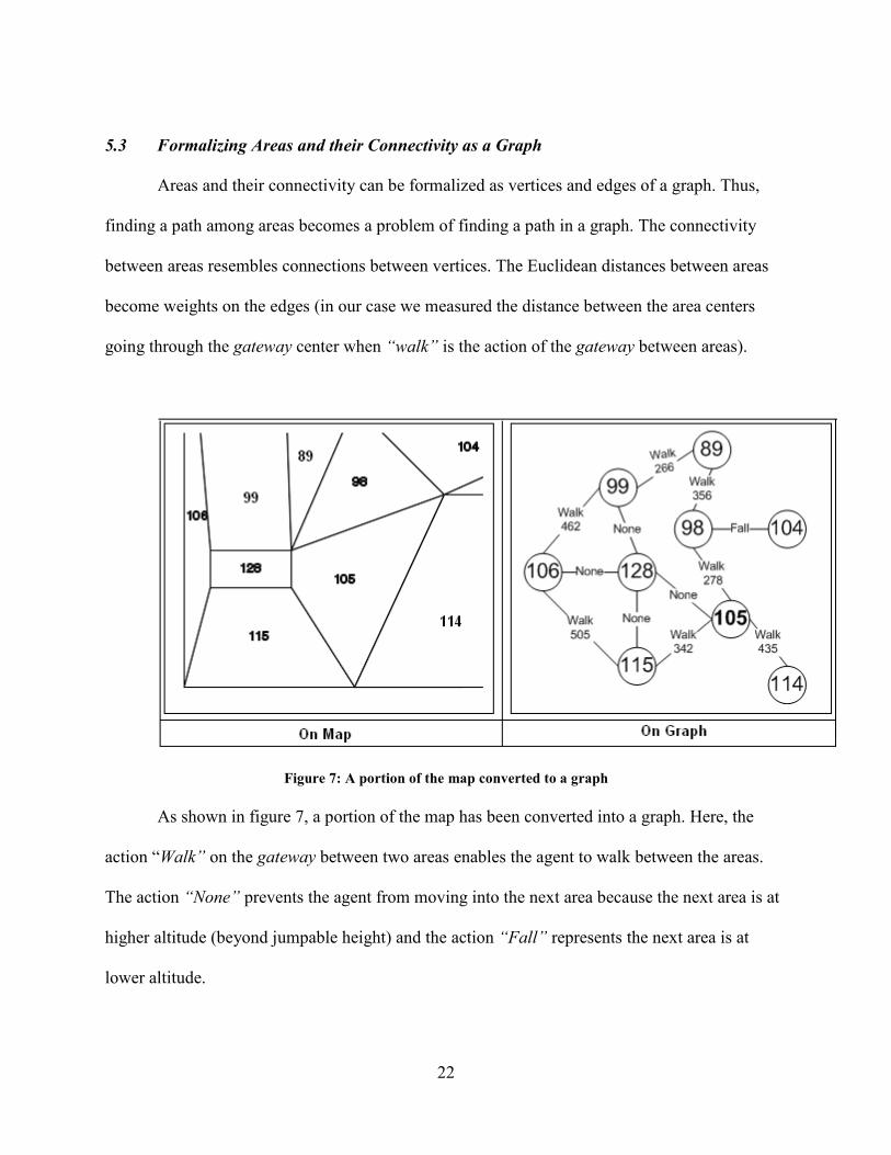
Figure 7: A portion of the map converted to a graph
As shown in figure 7, a portion of the map has been converted into a graph. Here, the
action “Walk” on the gateway between two areas enables the agent to walk between the areas.
The action “None” prevents the agent from moving into the next area because the next area is at
higher altitude (beyond jumpable height) and the action “Fall” represents the next area is at
lower altitude.
23
In our strategic path calculation we modify these weights to incorporate risk, and then use
the same shortest path algorithm to find a strategic path.
5.4 Strategic Path Calculation
Our strategic path calculations have been done by modifying the weights in the weight
matrix of the connectivity graph and then using the Dijkstra's algorithm to compute the shortest
paths. Each weight initially represents the Euclidean Distance between the area centers and it is
penalized for being exposed to an enemy. For this process we compute Meta-Weight for each
Weight.
The Meta-Weight is computed by computing the Hit Probability and the RiskVsTime
factor. The RiskVsTime is determined by the priority to safety for the agent in terms of mission
objectives. The Hit Probability is computed over the path connecting two area centers and that is
done by using checkpoint technique.

24
Figure 8: Strategic Distance is a trade-off between Risk and Time
In figure 8, the strategic path to the goal area is influenced by various factors like the fire
power of enemy’s weapon and priority given to survival over the time as per mission objectives.
A smaller RiskVsTime value (the smallest value is 0) means the safety has no priority. And
similarly a high RiskVsTime value means safety has a high priority and therefore any exposure to
enemies will be minimized. Thus, the strategic distance from an enemy will vary for an exposed
area.

25
Figure 9: In Strategic path computation tactical distance from a more dangerous enemy is maximized
Due to Hit Probability computation the tactical distances between a more and a less
dangerous enemy is computed fairly. In figure 9, the strategic distance between an enemy and
the agent depends on how dangerous the enemy is. For example an enemy with a sniper rifle is
considered more dangerous than an enemy with an assault rifle.
5.5 Abstraction of map into Areas
All the walkable surfaces have been converted into a small set of large convex polygonal
areas. There are a total of 227 areas out of which 169 areas are walkable (interconnected). And
also there are 43 different objects (buildings, garage, walls, pallets, bus-stop, street-lights, trees,
crates). Thus, for a small set of areas the graph representation and further application of shortest
path algorithm is computationally feasible. For complicated maps the concept of abstraction can
be further applied to a higher level. For example, we can define Zones, which are made up of
Areas and at a more detailed level we will have Grids. For example, in a map that contains

26
multiple buildings, to simplify details buildings can be considered as Zones and Floors can be
considered as Areas and further rooms can be considered as Grids.
5.6 Hit Probability (HP) Calculation
From a start area to a goal area there can be many paths. A path is defined by a set of
walkable polygonal areas. These areas can be visible to enemies. The risk factor of a path is
determined by calculating the total hit probability for all the areas along that path.
Figure 10: Hit probability based upon range modeled for three weapons.
The hit probabilities have been calculated from the realistic weapons data obtained from
[5]. As shown in figure 10, we considered 3 types of weapons: assault rifle (AK 47), sniper rifle
(SKS-84M) and sub-machine gun (MP5).
The realistic data gives a rough conversion of distances to static hit probability for
various weapons computed for a standing soldier. We convert the given static hit probability to
dynamic hit probability by considering it to be 0.25 (called DynamicRatio) times the static hit
27
probability. When the agent will be be moving, it will be harder to hit him, thus use a fraction of
the static hit probability to estimate the effects of the dynamics of the situation. If we don’t
consider DynamicRatio then it will be an unfair risk evaluation of a moving agent and also it will
lead to situations where many exposed paths will be considered equally risky because the total
hit probability over a path will consistently touch a high value (approx. 1.0) due to computational
limitation of floating point preciseness. Thus, the strategic path planning will fail to distinguish
between a less exposed and an over exposed path.
5.7 Checkpoints
A point on a path where the HP is computed has been defined as a checkpoint. In order to
calculate the hit probability associated with a path made of a set of points, the checkpoints are
linearly distributed along the path at a fixed Euclidean distance (called checkpoint length) and
finally the end point gets included (if the distance between the last checkpoint and the end point
was lesser than the checkpoint length). In the following equation HPtotal represents the total hit
probability over the given path and HPi represents the hit probability for a checkpoint. The total
hit probability is computed as:
HPtotal = HP1 + HP2.(1-HP1) + …HPn.(1-HPn-1).(1-HPn-2)…(1-HP1)
Where HP1, HP2 … HPn are the HPs of the checkpoints P1, P2 … Pn linearly distributed
along the path separated by checkpoint length. Here for instance (1-HP1) means probability of
not getting a hit on checkpoint P1 and HP2.(1-HP1) means the probability of only being hit on the
28
checkpoint P2. Similarly, HPn.(1-HPn-1).(1-HPn-2)…(1-HP1) represents the probability of only
taking a hit on the checkpoint HPn (after surviving hits over the previous checkpoints). Here we
focus only on the first hit, thus the probability of taking a hit only on a checkpoint is computed
from the product of probability of not getting hit over all the previous checkpoints and
probability of getting hit on that checkpoint. Thus, the total hit probability HPtotal represents
probability of getting a hit over all the checkpoints.
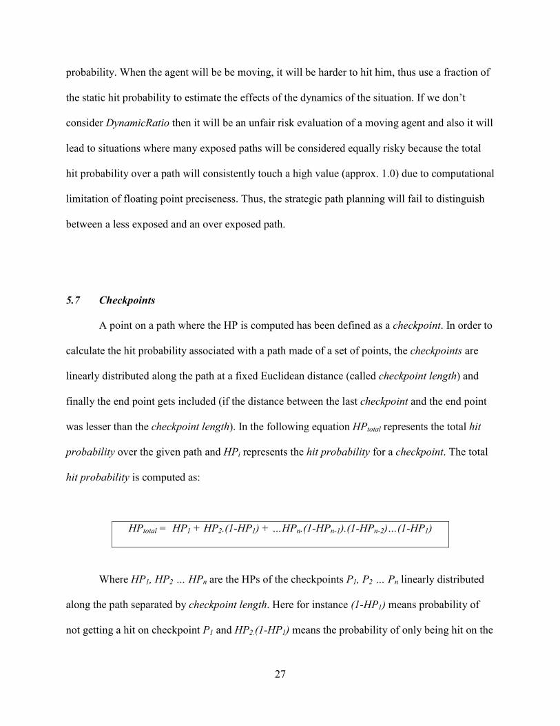
5.7.1 Checkpoints for Meta-weight computation
Figure 11: Checkpoint distribution along a pair of areas.
For the strategic path computation, each pair of neighboring areas is computed for the
risk. Here, the risk is the total hit probability along the checkpoints. As shown in figure 11 along
the thick dark line, the first checkpoint is allocated to the center of the start area, and the rest of

29
the checkpoints are distributed linearly (e.g. 1 meter checkpoint length) along the path to the
center of the stop area including the center of the stop area. This path goes through the
connecting gateway of the two neighboring areas. The hit probability (HP) over this path is used
for Meta-Weight computation. As shown in the figure 11 by the thick black marks.
5.7.2 Checkpoints for Risk Evaluation of a traced path
The path’s safety is computed using the hit probability over the path. And it is evaluated
by applying the checkpoint technique on the path. The shortest and strategic paths at Area level
are shown in figure 11 by the thin line (they are connected between the gateway centers). A
traced path is represented by a set of points. The start and the goal point are allocated a
checkpoint each and the checkpoints are linearly distributed at a fixed length (checkpoint length
1m) and the total hit probability is computed over these checkpoints using the checkpoint
technique as explained in section 5.7.
5.7.3 Comparison between Checkpoint techniques applied for Meta-Weight computation and
Risk Evaluation of a traced path

30
Figure 12: For paths traced the checkpoint count can be less
As shown in figure 12, It can be observed that the number of checkpoints computed
during meta-weight computation for the same path will always be more (or equal) than the
number of checkpoints computed in evaluating the risk on the path traced, because in the case of
the meta-weight calculation the checkpoint distribution is restarted for each pair of areas. And
when the checkpoint length is reduced, the correspondence between the total hit probability
across the area centers of the chosen Areas and the total hit probability across the computed
strategic path increases.
5.8 Visibility Constraints

31
Figure 13: The strategic path at Area level for Area-105
The strategic path computation at the Area level does not consider visibility information
within Areas at a great detail. In figure 13, Area-105 is considered on the basis of checkpoints
over the line segment joining its center and the Gateway point. Here, we constrain the visibility
considerations for the sake of reasoning that nobody can accurately predict the visibility
information within an Area at a very high degree without reaching it. Thus, it adds to efficiency
in the path calculations when an Area is considered at this abstraction, rather than reasoning
about all the points within an Area.
32
5.9 Risk vs. Time Preference Factor
Risk is attributed to the probability of being hit. In order to succeed on a mission the
agent must maintain a minimum health and minimize any health damage. This can be done by
taking a route that keeps the agent hidden from most of the threats on the map. But not all the
paths are threat free.
As per mission objectives the agent may want to reach a goal location as soon as
possible. For that the agent must take the shortest route towards the goal. But the shortest route
may contain threats. Thus, the agent must make a trade-off in selecting a path that can minimize
risks and time. Depending upon the mission objectives the preference for the shortest route
compared to preference for safety may vary. Thus, in order to maintain a good balance between
the safest path and the shortest path the agent must define its risk vs. time preference factor. A
high value will prioritize safety and a low value will prioritize time of traversal. For a higher the
RiskVsTime factor the strategic path computation would tend towards more safety thereby
decreasing the Output Hit Probability over the computed strategic path with a trade-off of a
longer route to the goal.
It can also be seen when RiskVsTime factor is 0 or when there is no enemy the strategic
path becomes the shortest path.
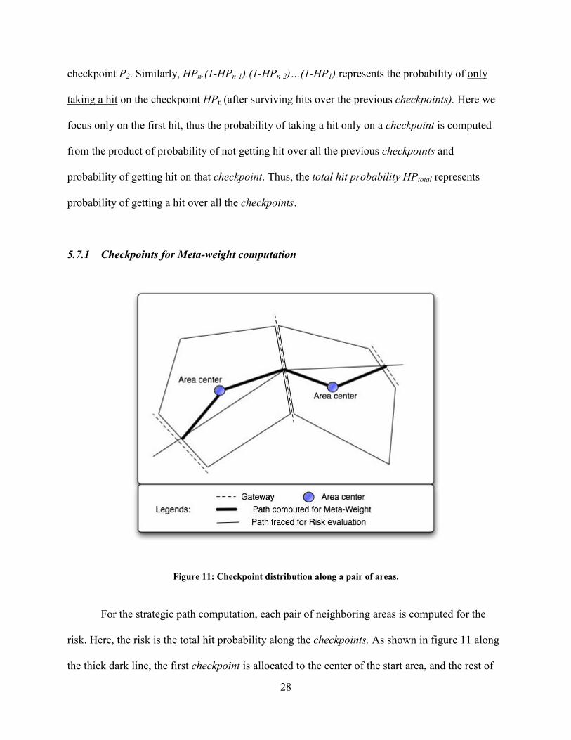
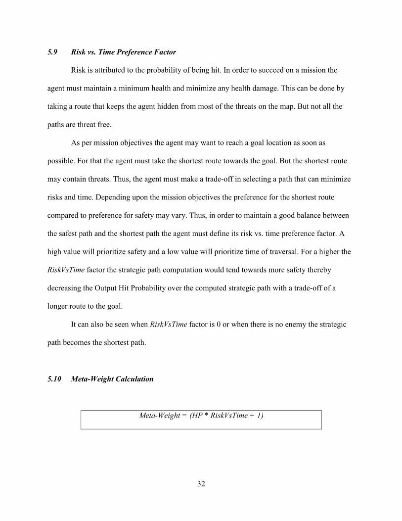
5.10 Meta-Weight Calculation
Meta-Weight = (HP * RiskVsTime + 1)

33
After determining the risk vs. time preference and the hit probability on the connecting
distance across the neighboring areas, we can compute a meta-weight. This meta-weight
represents a penalizing factor meant to symbolize the extra cost for being exposed to enemies.
In the formula an exposed area with the hit probability = 1 will be penalized linearly by
the RiskVsTime factor. So, the RiskVsTime = 1 factor will double the cost of traversal over that
area, whereas the RiskVsTime = 0 factor will keep the cost of traversal over that area unaffected,
thus any exposure will not affect any decision making.
5.11 Modification to the existing Weights
Weight = Meta-Weight * Euclidean Distance
The Euclidean distance is the distance between the centers of the areas passing through
the connecting gateway. Thus, all the weights are penalized for being exposed to the enemies.
5.12 Use of Shortest Path Algorithm
These meta-weights are multiplied to the Euclidean distances between the connected
areas. The computed weights are stored in an adjacency matrix. We use Dijkstra's single-pair-
shortest-path algorithm, because the computational complexity of the algorithm is O(n2).
Strategic path planning can also be done by using the Floyd-Warshall algorithm which
has the computation cost of O(n3). The main benefit for using the Floyd-Warshall algorithm is
that for further path planning the re-computation of the strategic path will not be required for
other pairs of areas as long as the enemy stays in the same location.

34
5.13 Strategic Path Calculation
The Shortest-Path algorithm is run on the above discussed computed weight and path
matrices. For each pair of areas we retrieve path information. The obtained path is the strategic
path, it balances the risk and the time as per mission requirements.
The algorithm 3 computes the strategic path at Area level. For each pair of areas it
computes the hit probability over the path joining their area centers through the gateway center
of their connecting gateway by using the checkpoint technique meant for computing Meta-
Weights (refer section 5.7.1). And then based upon the RiskVsTime determined by the preference
for the safety and then from the hit probability and RiskVsTime factor compute the Meta-Weight.
Then compute the product of the Meta-Weight and the Euclidean distance as the weight of an
edge. Compute all weights of the edges and use the shortest path algorithm to compute the
strategic path.
Algorithm 3: Strategic Path Planning at Area level Algorithm
INPUT: The static and the dynamic percepts.
OUTPUT: A set of Areas.
SYNOPSIS: Compute HP for each area pair and compute the Meta-Weight.
And for each edge take the product of Meta-Weight and the Euclidean
distance between their area centers (going through their gateway center).
The shortest path on this modified graph is the strategic path.
ALGORITHM:
1: Compute the HP from linearly distributed
checkpoints across each pair of the areas.
35
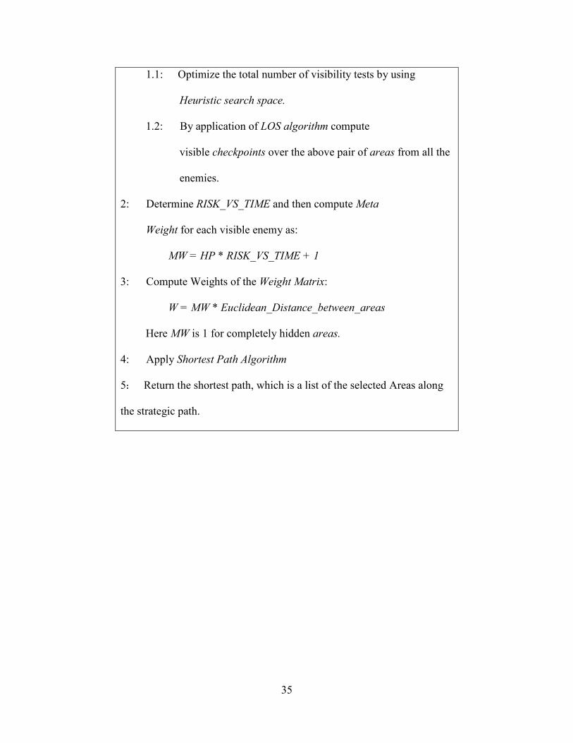
1.1: Optimize the total number of visibility tests by using
Heuristic search space.
1.2: By application of LOS algorithm compute
visible checkpoints over the above pair of areas from all the
enemies.
2: Determine RISK_VS_TIME and then compute Meta
Weight for each visible enemy as:
MW = HP * RISK_VS_TIME + 1
3: Compute Weights of the Weight Matrix:
W = MW * Euclidean_Distance_between_areas
Here MW is 1 for completely hidden areas.
4: Apply Shortest Path Algorithm
5: Return the shortest path, which is a list of the selected Areas along
the strategic path.

36
CHAPTER SIX
STRATEGIC PATH COMPUTATION AT GRID LEVEL
6.0 Overview
After the strategic path at the Area level is computed, the strategic path at the Grid level
(higher level of detail) is computed for each selected Area while traversing the selected Areas
computed by the strategic path at Area level. As shown in figure 12 a selected Area is further
divided using a grid formation (a rectangle of grid unit length). Here a bigger grid unit length
means more detail and more computational cost. This computation gives the within-area Grid
Points to walk through for each selected area. Thus, it takes into consideration any enemy
movement. A selected area is sub-divided using a Grid Formation, and a strategic path is
computed over the grid points. This technique is applied over all the chosen areas and it gives the
strategic path at Grid level.
37
Figure 14: The strategic path at Grid level for Area-105
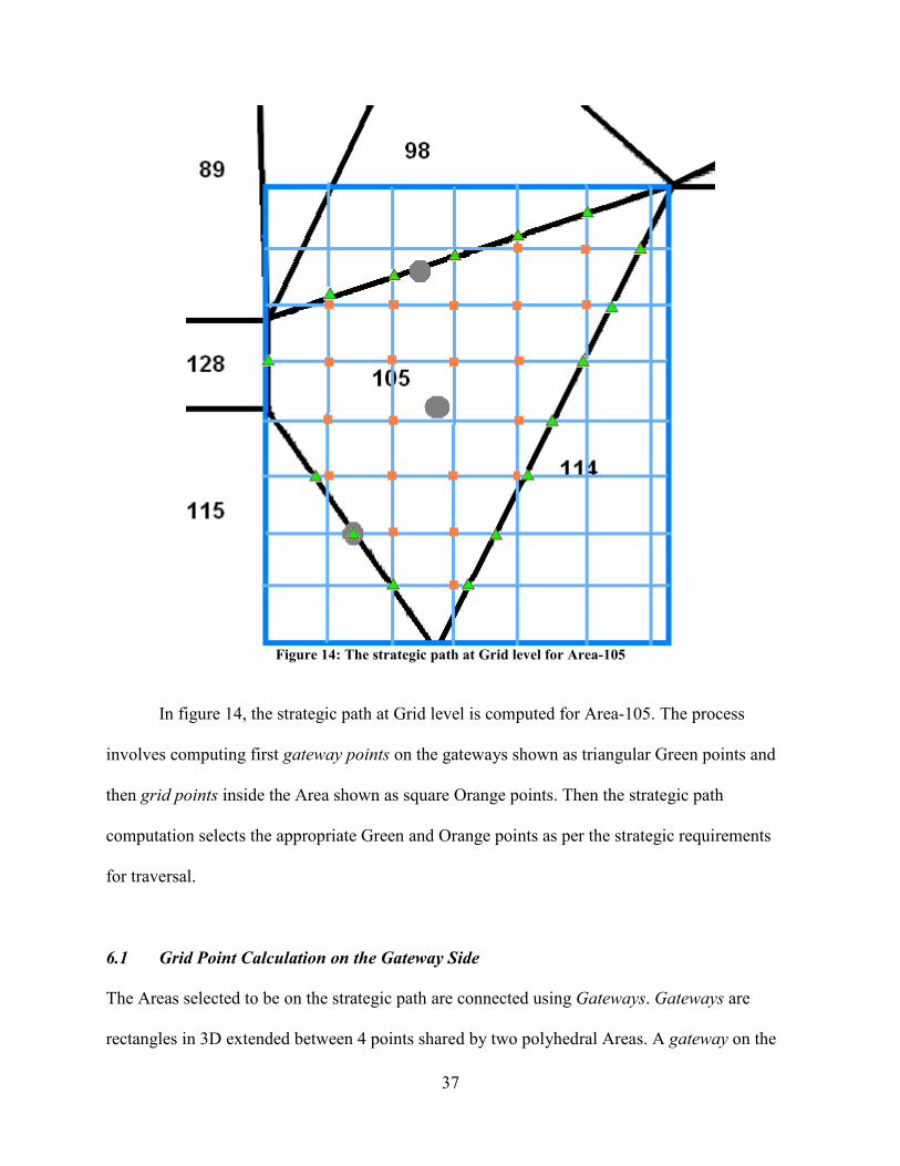
In figure 14, the strategic path at Grid level is computed for Area-105. The process
involves computing first gateway points on the gateways shown as triangular Green points and
then grid points inside the Area shown as square Orange points. Then the strategic path
computation selects the appropriate Green and Orange points as per the strategic requirements
for traversal.
6.1 Grid Point Calculation on the Gateway Side
The Areas selected to be on the strategic path are connected using Gateways. Gateways are
rectangles in 3D extended between 4 points shared by two polyhedral Areas. A gateway on the
38
Gateway side is computed using the below discussed algorithm. The selected Gateway Points on
the Gateway sides define the start and the end points of the strategic path at the Grid level for the
selected Area.
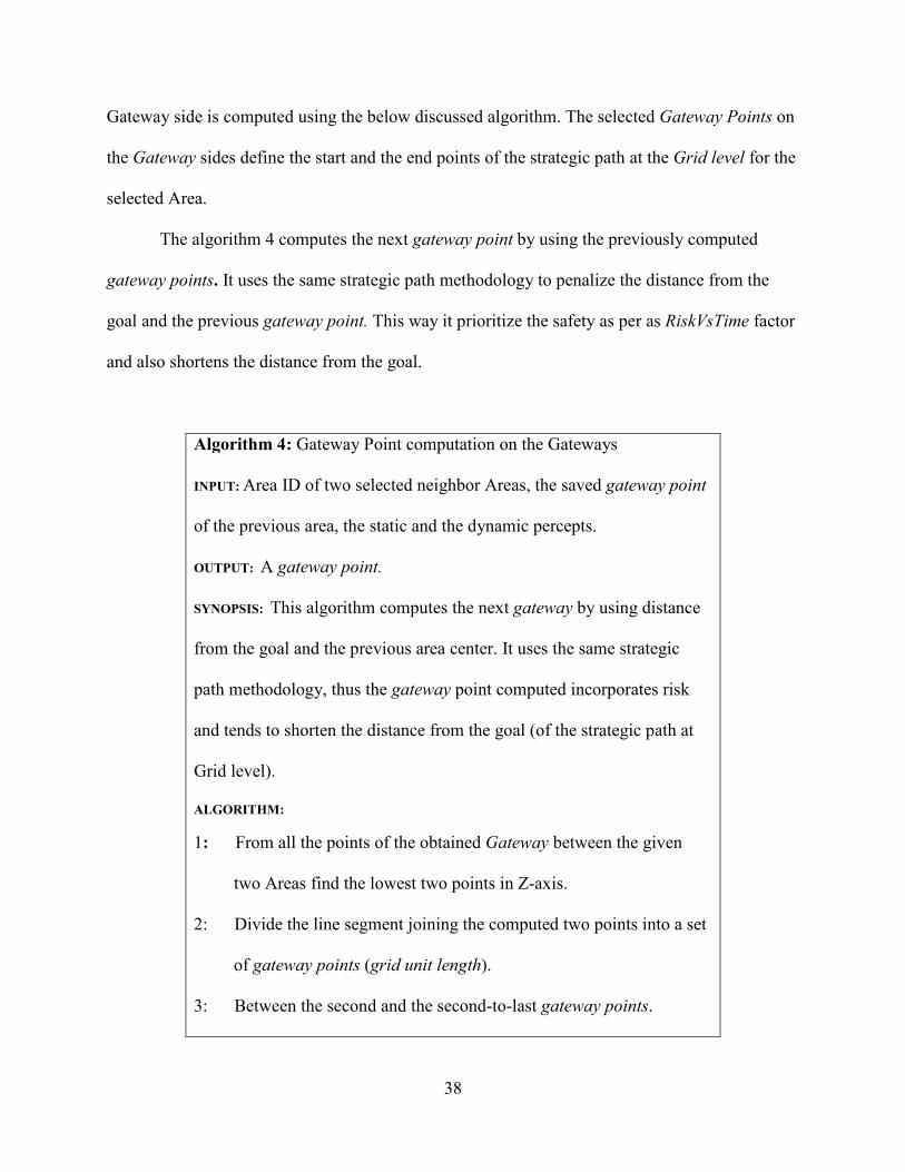
The algorithm 4 computes the next gateway point by using the previously computed
gateway points. It uses the same strategic path methodology to penalize the distance from the
goal and the previous gateway point. This way it prioritize the safety as per as RiskVsTime factor
and also shortens the distance from the goal.
Algorithm 4: Gateway Point computation on the Gateways
INPUT: Area ID of two selected neighbor Areas, the saved gateway point
of the previous area, the static and the dynamic percepts.
OUTPUT: A gateway point.
SYNOPSIS: This algorithm computes the next gateway by using distance
from the goal and the previous area center. It uses the same strategic
path methodology, thus the gateway point computed incorporates risk
and tends to shorten the distance from the goal (of the strategic path at
Grid level).
ALGORITHM:
1: From all the points of the obtained Gateway between the given
two Areas find the lowest two points in Z-axis.
2: Divide the line segment joining the computed two points into a set
of gateway points (grid unit length).
3: Between the second and the second-to-last gateway points.

39
Compute for each gateway point
MW = HP * RISK_VS_TIME + 1
Weight = MW * (EDgoal + EDprev-gateway_point)
Where HP is the hit probability of the gateway point.
Where EDgoal is the Euclidean distance from the goal.
Where EDprev-gateway_point is the Euclidean distance from the
selected gateway point of the previous Gateway between
the previous pair of two Areas on the same path.
4: Find the gateway point with the least weight among all the
gateway points considered above and return the coordinates of the
selected gateway point.
6.2 Grid Point Calculation inside the Selected Area
The strategic path at the Grid level produces a set of grid points that an agent can walk
over to traverse an area. These points are expected to meet strategic requirements of the agent.
From the above discussed algorithm a grid point is computed on the next gateway. Now, in
between the current point and the next gateway point over the bounded Area, a set of grid points
are computed by using the algorithm discussed below. This computation is done only when the
agent reaches the selected Area. Thus, the strategic path computation over the Area level gets a
list of selected Areas, and later while walking over these selected Areas, in accordance with the
enemy’s dynamic behavior, appropriate grid points are computed. As shown in algorithm 5.

40
The algorithm 5 computes the grid points inside an area. It takes two gateway points
(computed using algorithm 4) and it does the risk analysis inside an area at a great detail with
respect to any enemy’s current location and generates the strategic path at Grid level.
Algorithm 5: Grid Point computation inside an Area
INPUT: An Area and the two gateway points, the static and the dynamic
percepts.
OUTPUT: A list of grid points.
SYNOPSIS: This algorithm computes the strategic path at Grid level by
using the computed gateway points and the complete risk information for
all the grid points (by applying grid formation on the area). Then using the
same strategic path methodology of penalizing the exposed edges, it
generates the modified graph and by applying the shortest path algorithm a
set of grid points are generated to represent the strategic path at Grid level.
ALGORITHM:
1: Find the ground face (the lowest Z-axis) and then find
(Xmin , Ymin, Zmin) and (Xmax, Ymax, Zmax) of that face. And also find
which normal’s component (X or Y-axis) varies the most with Z-axis.
2: Store the sequence information of all the valid grid points that exists
inside the given Area by stepping through the computed
(Xmin , Ymin, Zmin) and (Xmax, Ymax, Zmax) in an optimized way inside a
2D integer array by:
2.1: Inside a rectangle formed by (Xmin , Ymin) and (Xmax, Ymax)

41
2.2: For Ymiddle between Ymin to Ymax iterate
2.3: Search for Xstart by iterating between Xmin to Xmax
Such that (Xstart, Ymiddle) is inside the Area.
2.4: Search for Xend by iterating between Xmax to Xmin
Such that (Xend, Ymiddle) is inside the Area.
2.5: For Xmiddle between Xstart to Xend
2.6 Store (Xmiddle , Ymiddle) as a valid grid point.
3: Formulate a graph where grid points are the vertices and their
connection among their neighbors are the edges. Each grid point is
connected with 8 neighbors (the nearest vertical, horizontal and
diagonal neighbors). The connection between two grid points is
computed as
MWGrid = HPGrid * RISK_VS_TIME + 1
WeightAB = EDAB * MWGrid
Where HPGrid is the hit probability across the two grid points.
Computed as HPGrid = HPA + HPB * (1 – HPA) where A and B
are the two grid points.
4: Associate the two end points to the grid point graph.
4.1: Find the closest grid point from each of the end points.
4.2: Add both the end points to the grid point graph as another
two vertices connected with the grid points computed
from step 4.1 with weights computed using step 3.
5: Now use Shortest Path algorithm (Dijkstra's algorithm) to find

42
the least-weight path between the two end points.
6: Along with the connected grid points, the two gateway points
are also connected with WeightGateways as its weight.
MWGateways = HPGateways * RISK_VS_TIME + 1
WeightGateways = EDGateways * MWGateways
Where HPGateways is the hit probability across the two selected
gateway points computed using checkpoint technique with
checkpoint length as the grid unit length.
Where EDGateways is the Euclidian Distance between the two
selected gateway points computed using checkpoint technique.
7: Compute grid point coordinates of the selected grid points on
the least cost path using slope information computed using
step 1 and cache the processed path information with respect to
the current enemy location for optimal future use.
The alternative connection between the two gateway points apart from the connection
over the selected grid points addresses two important cases. For the case, when there is no grid
point allocated to the Area and also for the case, when the Area is completely unexposed to any
of the enemies. The direct connection between the gateway points guaranties the shortest route
fairly computed with the alternative route through the selected grid points.
6.3 Risk calculation over the complete strategic path at Grid level

43
In the case of the strategic path calculation at Grid level. The path is tracked over the
selected grid points and gateway points computed for the chosen Areas computed by the
strategic path at Area level. This path can be evaluated for risk by using checkpoint technique
between the start and the end point through the selected grid points and gateway points.
44
CHAPTER SEVEN
EXPERIMENTATION AND VALIDATION
7.0 Overview
This chapter discusses our experiments and their results of out-game and in-game trials.
Section 7.1 discusses our experimental setups. Section 7.2 discusses one of the experiments with
the plots of the chosen strategic paths. Section 7.3 discusses variations in hit probability for
different weapons for out-game trials. Section 7.4 discusses an experiment with 50 runs of
different start area, end area and an enemy area with RiskVsTime = 10 and checkpoint length = 1
m for out-game trials. Section 7.5 addresses the hit probability variation between the Meta-
Weight computation and the traced path evaluation of the checkpoint technique. Section 7.6
discusses how the distances of the traced paths vary with RiskVsTime factor for the out-game
trials. Sections 7.7 to 7.9 discuss our in-game trial results. Section 7.10 discusses the in-game
trial results of the agent with shooting skills. Section 7.11 addresses some underlying
assumptions and discusses some observations.
7.1 Out-Game and In-Game experimental setup
We performed the Out-Game trials using the realistic weapon details [5]. By using the
checkpoint technique (refer section 5.7.2), we computed the hit probability of the generated
strategic paths. The In-Game trials were done on the UCT (a modification of Quake3). We ran
10 experiments and we took the average. For example in an experiment where the agent got hit 4
times and successfully reached without getting a hit 6 times had the hit probability of 0.4. We
performed the in-game trials to test the accuracy of the out-game computation.

45
7.1.1 Out-Game Trial Setup
Using the realistic weapon details [5], we used the checkpoint technique to evaluate the
risk factor involved to traverse the computed path. We modelled the three types of weapons (an
assault rifle, a sub-machine gun and a sniper rifle) and based upon the target distance, a hit
probability is computed. This computation is done over the set of checkpoints. In this process the
checkpoint distribution starts from the start location and ends at the goal location and between
these two points these checkpoints are linearly distributed using the checkpoint length.
7.1.2 In-Game Trial Setup
A scenario with a start location, a goal location and an enemy location were defined as an
experiment set. We ran 50 such experiments for the shortest path, the strategic path at Area level
and the strategic path at Grid level. And for each experiment we ran the same trial 10 times and
we computed the average HP for each of the three paths. The UCT is a modification of Quake3.
It does contain an implementation of realistic physics calculation up to a certain degree. Thus,
the gunshots were expected to have some realistic variations analogous to the real world. For the
above experiments we controlled an enemy bot and programmed it to shoot the agent. We
programmed the agent to walk between the start and the goal location along the computed
strategic path (using the shared memory access between the agent and the game).
Along the path of traversal the enemy bot tried to aim and shoot the agent, and for that
the enemy bot was given a very large count of ammunition (virtually infinite). We considered a
hit as a failure and moving from the start location to the goal location without getting any hit as a
success.

46
The in-game trials were based on the available shooting mechanism of the Quake3 game
engine (its simulated physics and its implementation of real world variations). The enemy bot
was controlled using the same shared memory mechanism (as of agent). Thus, the shooting
accuracy suffered many implementation level constraints like the yaw (bot’s angle on horizontal
plane) alignment where the bot is turned left/right until it reaches a desired threshold. The
weapon model we used to compute the Meta-Weights (the assault rifle) was different than the
existing shooting mechanism of the Quake3 game engine and therefore any variation among
them has a direct impact on the above in-game trials. The impact is subjective to how
consistently and accurately it matches the real-world weapon models, if the Quake3 engine
exhibits a poor range for a long range weapon then the strategic paths will meaninglessly take
longer distances and for other-way round situations the computed strategic paths will be more
risky than the computed risk values.
7.2 Experimental Results
47
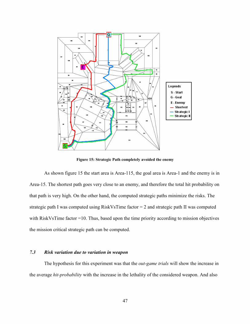
Figure 15: Strategic Path completely avoided the enemy
As shown figure 15 the start area is Area-115, the goal area is Area-1 and the enemy is in
Area-15. The shortest path goes very close to an enemy, and therefore the total hit probability on
that path is very high. On the other hand, the computed strategic paths minimize the risks. The
strategic path I was computed using RiskVsTime factor = 2 and strategic path II was computed
with RiskVsTime factor =10. Thus, based upon the time priority according to mission objectives
the mission critical strategic path can be computed.
7.3 Risk variation due to variation in weapon
The hypothesis for this experiment was that the out-game trials will show the increase in
the average hit-probability with the increase in the lethality of the considered weapon. And also

48
the out-game trials will show the increase in the average hit-probability for all the three
considered weapons with the increase in the count of enemies.
Figure 16: Plots of variations in Avg. Output Hit Probabilities with different weapons
The figure 16 shows the average output hit probabilities due to different weapons. As
discussed in chapter 5.6, the Assault Rifle has the lowest lethality in terms of hit accuracy. Thus,
the average output hit probability computed is less than the other two considered weapons. For
the case of two enemies, a significant portion of the map becomes risky, resulting in a higher
average output hit probability. And we can also see the grid paths were consistently safer than
strategic paths and shortest paths for all types of weapons.
The hypothesis for this experiment was confirmed. We found with the increase in the
lethality of the considered weapon the average hit probability increased. And also found that
with the increase in the number of enemy count the average hit probability increased. The
hypothesis for this experiment tested the accuracy of the out-game trial.
49
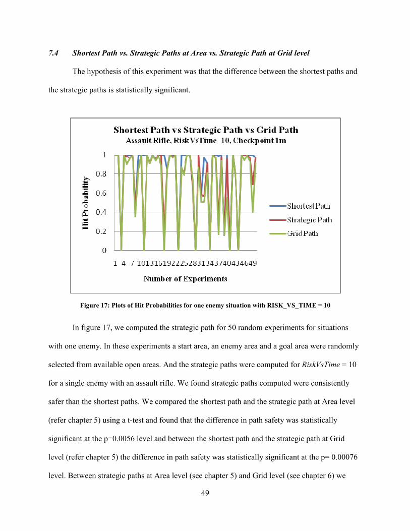
7.4 Shortest Path vs. Strategic Paths at Area vs. Strategic Path at Grid level
The hypothesis of this experiment was that the difference between the shortest paths and
the strategic paths is statistically significant.
Figure 17: Plots of Hit Probabilities for one enemy situation with RISK_VS_TIME = 10
In figure 17, we computed the strategic path for 50 random experiments for situations
with one enemy. In these experiments a start area, an enemy area and a goal area were randomly
selected from available open areas. And the strategic paths were computed for RiskVsTime = 10
for a single enemy with an assault rifle. We found strategic paths computed were consistently
safer than the shortest paths. We compared the shortest path and the strategic path at Area level
(refer chapter 5) using a t-test and found that the difference in path safety was statistically
significant at the p=0.0056 level and between the shortest path and the strategic path at Grid
level (refer chapter 5) the difference in path safety was statistically significant at the p= 0.00076
level. Between strategic paths at Area level (see chapter 5) and Grid level (see chapter 6) we
50
found the difference in path safety was statistically significant at the p=0.00085 level. This
confirms the claim when seen in abstraction an Area gives a rough estimation about its safety
and when that Area is reached and when the Grid Path is computed for that Area then it can be
consistently traversed with same or lesser risk.
We can expect anomalies where the shortest path can be evaluated as less costly (i.e.,
safer) than the strategic paths. This is because for Meta-Weight computation, more checkpoints
are distributed along the Areas and when the strategic path is obtained along the same set of
Areas it contains lesser checkpoints. During safety evaluation if a portion of a computed strategic
path is exposed and on the other hand if the shortest path gets lesser checkpoints exposed due to
variation in checkpoint distribution along the exposed areas then this could result into a situation
where a strategic path could get evaluated to have a higher hit probability compared to the
shortest path.
The hypothesis for this experiment was confirmed. We also found the difference between
the strategic path at Area level and the strategic path at Grid level was also statistically
significant.
7.5 HP variation between Meta-Weight computation and Path traced evaluation
The hypothesis of this experiment was with the increase of the RiskVsTime factor the
generated strategic paths will become safer and also with the decrease in the checkpoint length
the difference between hit probabilities computed by the checkpoint technique for Meta-Weight
computation and risk evaluation of the traced path will decrease.
The checkpoint technique computes the Hit Probability between the Area centers of each
of the neighboring Areas for Meta-Weight computation. Both the Area centers get one

51
checkpoint each and checkpoints are linearly distributed along the path joining the two Area
centers through the gateway center. The number of checkpoints distributed using this technique
is always more than the number of checkpoints distributed across the start and the goal point for
the strategic paths.
Figure 18: HP variation between Meta-Weight computation and Path’s risk evaluation for 1m checkpoint
In figure 18, the relation between Meta-Weight HP and computed Paths has been plotted
with respect to RiskVsTime factor. As RiskVsTime factor increases the hit probability (HP)
decreases and thereby the computed path becomes safer. And it can be seen that Grid Paths are
consistently safer compared to other paths. The RiskVsTime factor has no-effect on the shortest
path.

52
Figure 19: HP variation between Meta-Weight computation and Path’s risk evaluation for 0.5 checkpoint
In figures 18 and 19, when checkpoints are of smaller lengths the difference between HP
for Meta-Weight and Path’s risk evaluation significantly reduces and they tend to approach
higher values compared to shorter checkpoint lengths.
The hypothesis of this experiment was confirmed. We found with the increase of
RiskVsTime factor the generated strategic paths were safer and also with the decrease in the
checkpoint length the difference between the hit probabilities computed by the checkpoint
technique for Meta-Weights and risk evaluation of the traced path decreased. And we also found
the overall hit probabilities for all the traced paths and for the Meta-Weight computation
increased with the decrease in the checkpoint length.
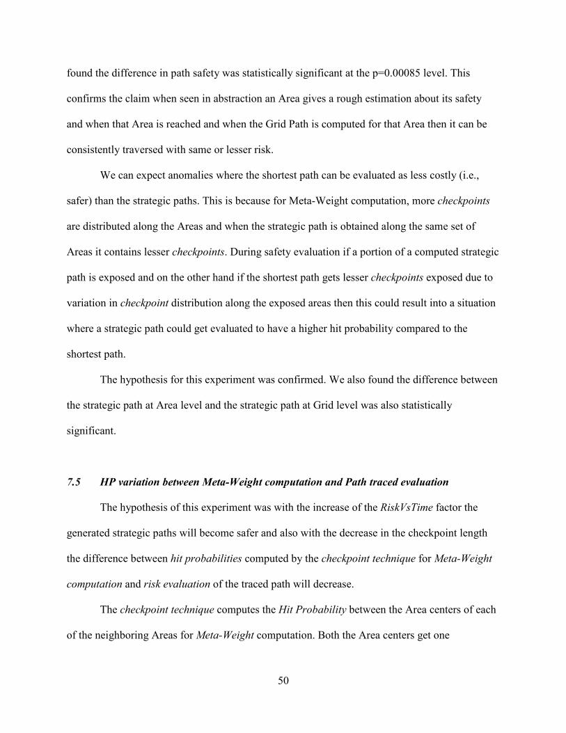
7.6 Distance variation between shortest, strategic paths at Area and Grid level
53
The hypothesis of this experiment was with the increase in the RiskVsTime factor the
distance of traversal will increase.
Figure 20: Avg. distance of shortest paths, strategic paths over Area and Grid level
In figure 20, for out-game trials as the RiskVsTime factor increases the strategic paths
become safer at a cost of longer distances. The strategic path computation selects the shortest
penalized path and in this process it tends to minimize both the risk and the distance of traversal.
In the case of the strategic path at Area level the distance is the shortest distance between the
gateway points lying at the centers of Gateways. And in the case of the strategic path at Grid
level, these gateway points tend toward the goal Area and strive to remain smooth over the
irregular Areas (using a similar A* technique). As a result the distance is further minimized.
54
The hypothesis of this experiment was confirmed. We also found the strategic path at
Grid level was shorter than the strategic path at Area level.
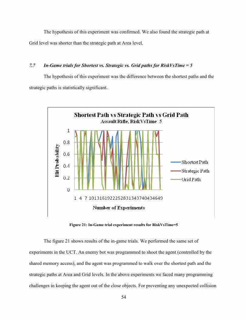
7.7 In-Game trials for Shortest vs. Strategic vs. Grid paths for RiskVsTime = 5
The hypothesis of this experiment was the difference between the shortest paths and the
strategic paths is statistically significant.
Figure 21: In-Game trial experiment results for RiskVsTime=5
The figure 21 shows results of the in-game trials. We performed the same set of
experiments in the UCT. An enemy bot was programmed to shoot the agent (controlled by the
shared memory access), and the agent was programmed to walk over the shortest path and the
strategic paths at Area and Grid levels. In the above experiments we faced many programming
challenges in keeping the agent out of the close objects. For preventing any unexpected collision

55
with close objects we used the HSS technique to determine the set of objects associated with the
HSS element representing the current Area, and we programmed the agent to walk along the
close objects and walls by maintaining a small distance. We found that there were very few
random occasions (1 in 500) when the agent or the enemy bot got stuck and could not recover.
We marked those experiments as undecided.
For RiskVsTime = 5, we ran the same set of 50 experiments and compared the shortest
path and the strategic path at Area level (refer chapter 5) using a t-test and found that the
difference in path safety was statistically significant at the p= 0.0024 level for the in-game trials.
Between the shortest path and the strategic path at Grid level (refer chapter 5) the difference in
path safety was statistically significant at the p= 0.0013 level for the in-game trials. Between
strategic paths at Area level (see chapter 5) and Grid level (see chapter 6) we found the
difference in path safety was not statistically significant at the p= 0.119 level for the in-game
trials.
The hypothesis of this experiment was confirmed. We also found the difference between
the strategic path at Grid level and the strategic path at Area level was also statistically
significant.
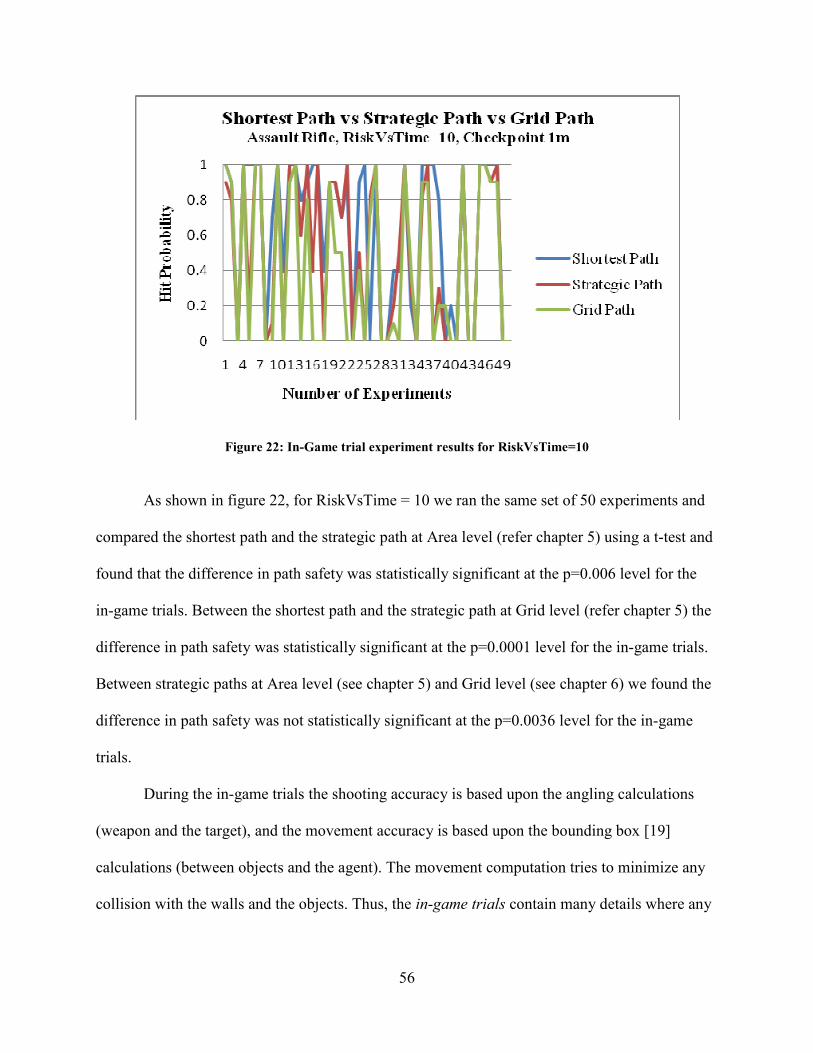
7.8 In-Game trials for Shortest vs. Strategic vs. Grid paths for RiskVsTime = 10
The hypothesis of this experiment was the difference between the shortest paths and the
strategic paths is statistically significant.
56
Figure 22: In-Game trial experiment results for RiskVsTime=10
As shown in figure 22, for RiskVsTime = 10 we ran the same set of 50 experiments and
compared the shortest path and the strategic path at Area level (refer chapter 5) using a t-test and
found that the difference in path safety was statistically significant at the p=0.006 level for the
in-game trials. Between the shortest path and the strategic path at Grid level (refer chapter 5) the
difference in path safety was statistically significant at the p=0.0001 level for the in-game trials.
Between strategic paths at Area level (see chapter 5) and Grid level (see chapter 6) we found the
difference in path safety was not statistically significant at the p=0.0036 level for the in-game
trials.
During the in-game trials the shooting accuracy is based upon the angling calculations
(weapon and the target), and the movement accuracy is based upon the bounding box [19]
calculations (between objects and the agent). The movement computation tries to minimize any
collision with the walls and the objects. Thus, the in-game trials contain many details where any
57
technical inaccuracy could have a negative impact on the results. On the other hand for the case
of out-game trials these game details are abstracted and do not adversely affect the analysis.
The hypothesis of this experiment was confirmed. We also found the difference between
the strategic path at Grid level and the strategic path at Area level was also statistically
significant. The importance of the in-game trials was to check the accuracy of the strategic path
computation model and we found the model was consistent with the in-game trials.
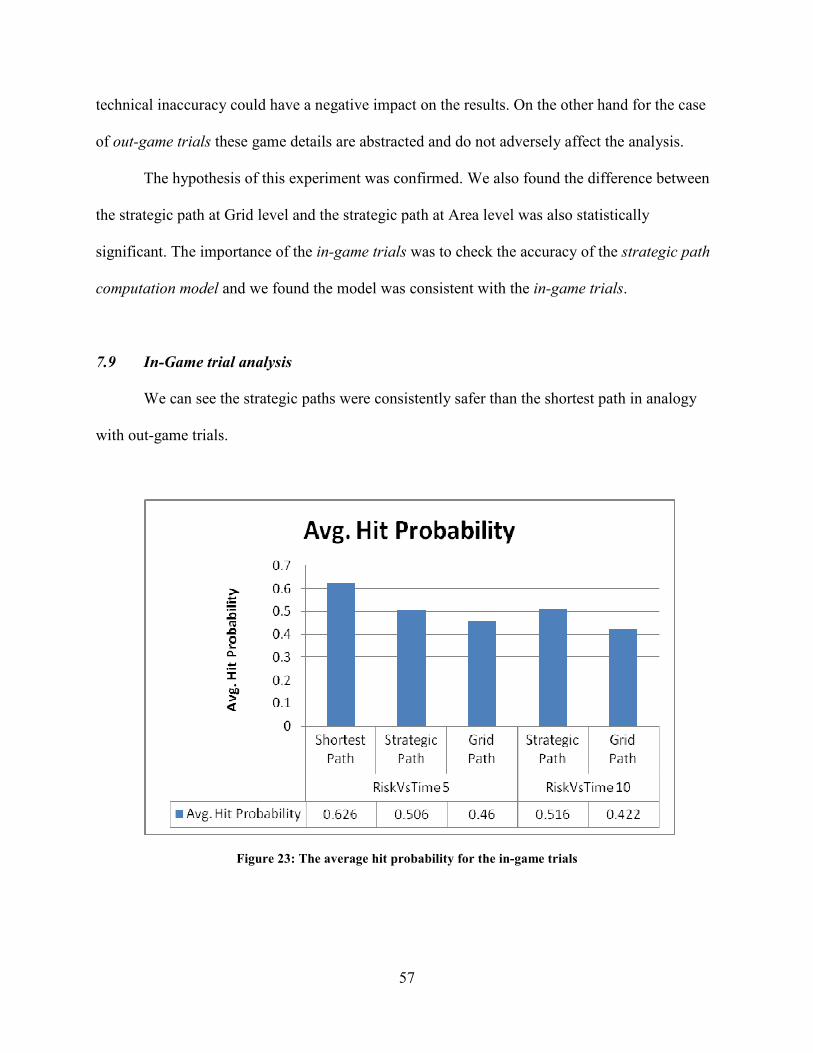
7.9 In-Game trial analysis
We can see the strategic paths were consistently safer than the shortest path in analogy
with out-game trials.
Figure 23: The average hit probability for the in-game trials

58
We can see in figure 23 that the Strategic Path at Grid level had the lowest hit probability
for both the RiskVsTime factors. We also see when RiskVsTime factor increased from 5 to 10 the
hit probability for Strategic Path at Grid level decreased from 0.46 to 0.422 in analogy to out-
game trials. The average hit probability for Strategic Path at Area level increased when
RiskVsTime increased from 5 to 10. We further analysed the above experiments and we learned
that there were 6 cases where the paths (a set of Areas) suggested by RiskVsTime 10 was
different from the paths suggested by RiskVsTime 5 and in these paths we found the path
computed by RiskVsTime 10 were safer. The left 44 paths were the same for both RiskVsTime
factors and we found the paths computed by RiskVsTime 10 suffered more hits compared to
paths suggested by RiskVsTime 5. The Quake3 engine tries to follow the real-world variation
through their projectile and simulated physics implementation and in above situation we can see
for the same 44 runs the agent suffered a little variation as per their variation implementation.
We also see even though the Grid paths were consistently of shorter length than the
Strategic paths (refer figure 19), we found that on the Grid paths the agent spent more time than
the corresponding longer Strategic paths (as shown in figure 23). In figure 23, failed paths
(where the agent could not reach the goal area) have been considered to take 0 seconds.

59
Figure 24: Avg. Time of Successful walks of Strategic and Grid Paths
In the Grid paths the agent tries to get closer to the walls to minimize exposure and
maximize the distance from the enemy, but the technique we applied to prevent the agent from
hitting the wall required the agent to change its movement angle continuously in order to avoid
getting stuck. While the agent turns, it has the lowest or almost no speed and therefore it walks
along the walls with a very slow speed (because of intermittent turns) and on many occasions
this results in more time to traverse (as shown in figure 24).
7.10 In-Game Trials of Agent with shooting skills
The hypothesis of this experiment was the agent with shooting skills on the strategic path
will perform better than the agent on the shortest path.
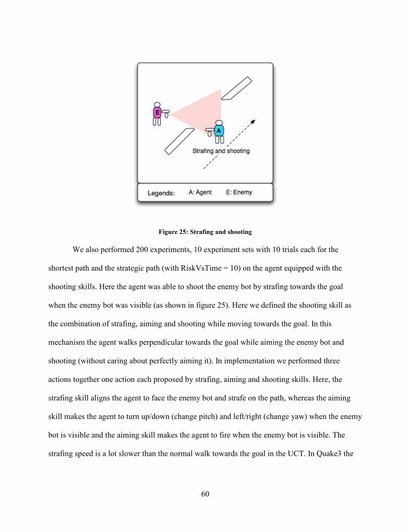
60
Figure 25: Strafing and shooting
We also performed 200 experiments, 10 experiment sets with 10 trials each for the
shortest path and the strategic path (with RiskVsTime = 10) on the agent equipped with the
shooting skills. Here the agent was able to shoot the enemy bot by strafing towards the goal
when the enemy bot was visible (as shown in figure 25). Here we defined the shooting skill as
the combination of strafing, aiming and shooting while moving towards the goal. In this
mechanism the agent walks perpendicular towards the goal while aiming the enemy bot and
shooting (without caring about perfectly aiming it). In implementation we performed three
actions together one action each proposed by strafing, aiming and shooting skills. Here, the
strafing skill aligns the agent to face the enemy bot and strafe on the path, whereas the aiming
skill makes the agent to turn up/down (change pitch) and left/right (change yaw) when the enemy
bot is visible and the aiming skill makes the agent to fire when the enemy bot is visible. The
strafing speed is a lot slower than the normal walk towards the goal in the UCT. In Quake3 the

61
yaw defines the aiming angle.When the agent strafes or moves, the yaw changes and the aiming
is affected.
The enemy bot was programmed to aim and shoot the agent. On a successfully killing of
the enemy bot the agent was programmed to switch to the shortest path to the goal area.
7.10.1 Agent with shooting skills
Figure 26: Safely reached experiment count analysis of agent with shooting skills
The strategic paths (Area level) were computed with RiskVsTime = 10. As shown in
figure 25, on 23 occasions the agent safely reached the goal area while traversing the shortest
path compared to 33 occasions while traversing the strategic path.
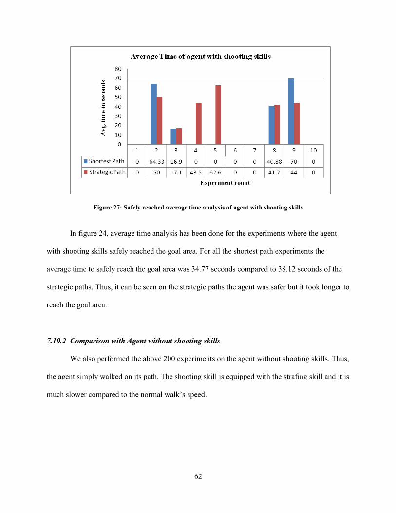
62
Figure 27: Safely reached average time analysis of agent with shooting skills
In figure 24, average time analysis has been done for the experiments where the agent
with shooting skills safely reached the goal area. For all the shortest path experiments the
average time to safely reach the goal area was 34.77 seconds compared to 38.12 seconds of the
strategic paths. Thus, it can be seen on the strategic paths the agent was safer but it took longer to
reach the goal area.
7.10.2 Comparison with Agent without shooting skills
We also performed the above 200 experiments on the agent without shooting skills. Thus,
the agent simply walked on its path. The shooting skill is equipped with the strafing skill and it is
much slower compared to the normal walk’s speed.
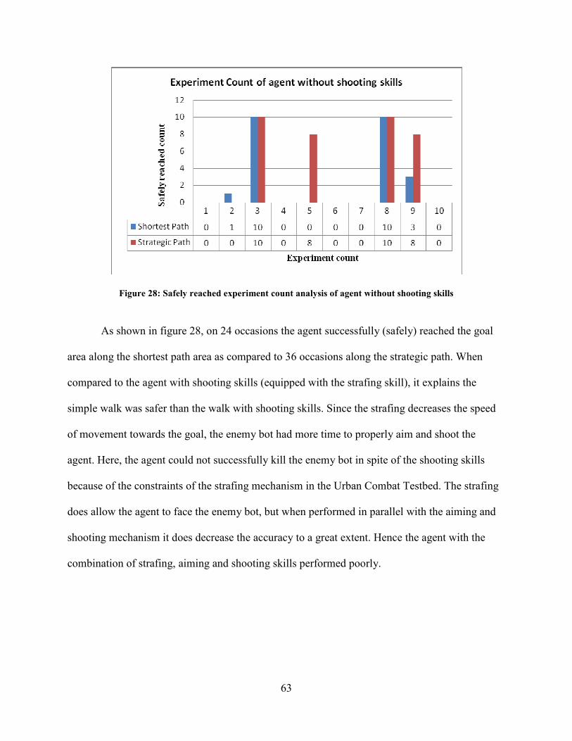
63
Figure 28: Safely reached experiment count analysis of agent without shooting skills
As shown in figure 28, on 24 occasions the agent successfully (safely) reached the goal
area along the shortest path area as compared to 36 occasions along the strategic path. When
compared to the agent with shooting skills (equipped with the strafing skill), it explains the
simple walk was safer than the walk with shooting skills. Since the strafing decreases the speed
of movement towards the goal, the enemy bot had more time to properly aim and shoot the
agent. Here, the agent could not successfully kill the enemy bot in spite of the shooting skills
because of the constraints of the strafing mechanism in the Urban Combat Testbed. The strafing
does allow the agent to face the enemy bot, but when performed in parallel with the aiming and
shooting mechanism it does decrease the accuracy to a great extent. Hence the agent with the
combination of strafing, aiming and shooting skills performed poorly.

64
Figure 29: Safely reached average time analysis of agent without shooting skills
In the figure 29, average time analysis has been done for the experiments where the agent
without shooting skills safely reached the goal area. For all the shortest path experiments the
average time to safely reach the goal area was 26.2 seconds compared to 35.69 seconds of the
strategic paths. Thus, it can be seen on the strategic paths the agent was safer but it took longer to
reach the goal area. And when compared to the agent with the shooting skills we can see the
slow speed of strafing caused more failures.
Since there is no separate aiming mechanism other than the yaw itself, any movement
towards the right direction (strafing or forward walk towards the goal) requires the yaw to
change and it affects the Aiming and the Shooting accuracy. Due to the limitations of no separate
Aiming angle the two parallel actions Strafing and Aiming interfere with each other and decrease
the shooting accuracy of the agent.
In above experiments, we have considered a stationary enemy bot. When the agent shoots
the enemy bot it stays in the same location. Here, we can model the enemy bot to move to a safe

65
location when the agent bot fires a few rounds. Thus, the enemy bot will get a short interval to
shoot the agent, and if it misses, then it will take cover and stop shooting. For above experiments
this modeling will improve the hit probability of the agent.
Figure 30: Strafe, aim, shoot and take cover.
As shown in the figure 30, we can also consider the agent to be stationary for a while and
just perform aiming and shooting operations for a short interval and then take cover by strafing
back to the previous location if the path towards the goal can be traced without getting a hit.
The hypothesis of this experiment was confirmed. And we also found the agent couldn’t
improve its performance with the shooting skills because of the limitations of the Quake3 engine
(it uses yaw for both movement and aiming).
7.11 Observation
In this chapter we performed many out-game and in-game trials. We computed the
variance between the in-game and out-game trials (hit probabilities for the traced paths) with
66
RiskVsTime 10 and Assault Rifle for the strategic path at Area level and it was found 0.17761
and for the strategic path at Grid level it was found 0.1896. The variances between the in-game
and the out-game trials for the strategic paths are good considering the gap of real-world weapon
performance and Quake3’s implementation of a similar weapon (similar but not the same). The
out-game trials were based upon the realistic risk evaluation computed from available weapon
details and it was free from the implementation details of the Quake3 game engine. We
performed out-game trials with variation in RiskVsTime factor from 0 to 30. We observed that
the computed strategic paths (Area and Grid levels) for a high RiskVsTime factor were
consistently safer. We found the strategic paths at Grid level were safest among the three paths.
And we also observed the Grid paths were of shorter lengths, but in in-game trials it took more
time to trace these paths compared to the Strategic paths. We also analyzed the effect of variation
in checkpoint length and observed for a shorter checkpoint length the hit probability computed
for Meta-Weights was closer to the paths’ evaluated hit probability. We performed experiments
on the agent with shooting skills and observed the limitation that using the same yaw for aiming
and movement caused the agent to perform poorly with the strafing/shooting skills.
67
CHAPTER EIGHT
OTHER APPLICATIONS OF STRATEGIC PATH PLANNING
8.0 Overview
This chapter discusses about the use of strategic path planning. The above strategic path
computation can also be used for implementing various for Military Operations on Urban Terrain
(MOUT) strategies and tactics. Flanking [4, 13] can be done by constructing a strategic path that
minimizes exposure to other enemies while targeting a specific enemy. Ambush [4] can also be
used by an agent by moving early to an area without being seen and waiting in anticipation of an
enemy. Later this chapter discusses about possible further improvements in the strategic path
planning and its implementation requirements. And this chapter also discusses how it can be
used with Real Time Strategy (RTS) games.
8.1 Basic Strategic Tactics
In the basic strategic tactics (as shown in figure 31) the agent just targets a specific
enemy without getting exposed to the other enemies.
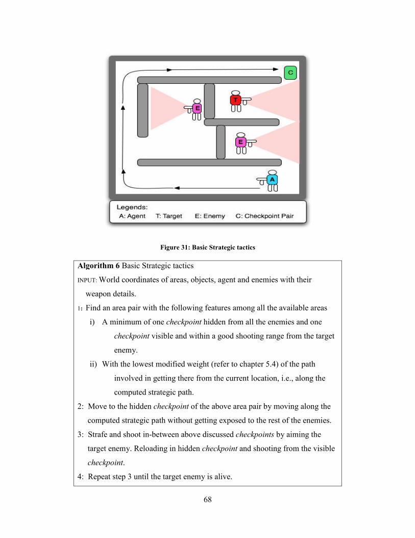
68
Figure 31: Basic Strategic tactics
Algorithm 6 Basic Strategic tactics
INPUT: World coordinates of areas, objects, agent and enemies with their
weapon details.
1: Find an area pair with the following features among all the available areas
i) A minimum of one checkpoint hidden from all the enemies and one
checkpoint visible and within a good shooting range from the target
enemy.
ii) With the lowest modified weight (refer to chapter 5.4) of the path
involved in getting there from the current location, i.e., along the
computed strategic path.
2: Move to the hidden checkpoint of the above area pair by moving along the
computed strategic path without getting exposed to the rest of the enemies.
3: Strafe and shoot in-between above discussed checkpoints by aiming the
target enemy. Reloading in hidden checkpoint and shooting from the visible
checkpoint.
4: Repeat step 3 until the target enemy is alive.

69
8.2 Shoot and Scoot
In Shoot and Scoot MOUT tactics (as shown in figure 32) the agent varies its shooting
location from one point to another point without getting noted by other enemies. In this process
the agent goes on changing the shooting location to prevent losses due to any heavy retaliation.
Figure 32: Shoot and Scoot tactics
Algorithm 7 Shoot and Scoot MOUT tactics
INPUT: World coordinates of areas, objects, agent and enemies with their weapon
details.
1: Find an area pair with following features among all the available areas
i) A minimum of one checkpoint hidden from all the enemies and one
checkpoint visible and within a good shooting range from the target
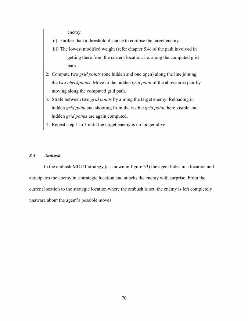
70
enemy.
ii) Farther than a threshold distance to confuse the target enemy.
iii) The lowest modified weight (refer chapter 5.4) of the path involved in
getting there from the current location, i.e. along the computed grid
path.
2: Compute two grid points (one hidden and one open) along the line joining
the two checkpoints. Move to the hidden grid point of the above area pair by
moving along the computed grid path.
3: Strafe between two grid points by aiming the target enemy. Reloading in
hidden grid point and shooting from the visible grid point, here visible and
hidden grid points are again computed.
4: Repeat step 1 to 3 until the target enemy is no longer alive.
8.3 Ambush
In the ambush MOUT strategy (as shown in figure 33) the agent hides in a location and
anticipates the enemy in a strategic location and attacks the enemy with surprise. From the
current location to the strategic location where the ambush is set, the enemy is left completely
unaware about the agent’s possible moves.

71
Figure 33: Ambush MOUT strategy

72
Algorithm 8 Ambush MOUT tactics
INPUT: World coordinates of areas, objects, agent and enemies with their weapon
details.
1: Find the strategic area (an area with no nearby cover)
where the target enemy is anticipated.
i) It can be an area on a path towards power-ups or something important to
the target enemy.
ii) If the target enemy is returning from a locked area and this area exists on
one and only one path.
iii) This strategic area should also fulfill (2).
2: The agent should be able to reallocate to an area pair (as discussed below)
within the walkable range from the agent’s current location. This area pair
should have
i) A minimum of one checkpoint hidden from all the enemies and one
checkpoint visible and within a good shooting range from the target
strategic area.
ii) The lowest weight (refer chapter 5.4) involved in getting there from the
current location, i.e. along the computed strategic path. (To prevent
any harm from other enemies).
III) And it should be completely hidden from all the areas the enemy is
expected to move along to reach the above discussed strategic area.
3: The agent should move to the hidden checkpoint by moving along a computed
grid path (with a very high value of RiskVsTime) and wait until the
enemy appears in the strategic area.
4: Strafe and shoot in-between dynamic grid points computed for above
discussed checkpoints by aiming the target enemy. Reloading in a hidden grid
point and shooting from the visible grid point.
5: Repeat step 4 until the target enemy is alive.
73
CHAPTER NINE
CONCLUSION AND FUTURE WORK
9.0 Overview
This chapter discusses about our conclusions and addresses how the concept of
abstraction and concept of detailed dynamic visibility calculation at run-time for realistic risk
calculation could be used to for both efficiency and more accurate risk analysis of a path. It also
addresses issues related with using A* technique. It also discusses the applicability of our
proposed strategic path computation algorithm in a more generalized for other computer science
related fields and real world problems. And later this chapter discusses about the future work.
9.1 Conclusion
We studied three important components of risk on a path of traversal. It is not just an
issue of exposure, but the distance from the enemies and their lethality also determine the real
risk. A strategic path calculation must penalize paths by considering all three components of risk
and making a proper trade-off between risk vs. time. We also studied how strategic path at Area
level does the risk evaluation of an Area at an abstraction and in turn that adds to efficiency in
computation. Therefore, the dynamic visibility calculation for areas is feasible at run-time and
more accurate since it is based on the enemy's exact location. This also makes it possible to
consider dynamic objects.
When the agent reaches the computed Area, the strategic path is computed over the Grid
Points of that Area. Thus, the calculation of the hit probability can take into account the real-time
movements of the enemies as the agent traverses the Grid Points of an Area.
74
By doing computation at two levels the strategic path computation is linearly distributed
over the complete traversal process and therefore it does not become computationally intensive.
Secondly, in addition to the computational savings of calculating strategic paths at the
Area level, rather than the Grid level (or using Waypoints), there is also the issue of not knowing
visibility details within an Area until the agent arrives at that Area, especially in urban combat
settings. Thus the agent exhibits intelligence (in strategic path computation) in a more realistic
way.
The strategic path planning at Area level can be further abstracted to a more abstract
concept called Zones (discussed in chapter 5.5) for more complicated maps. Thus the strategic
path planning will perform at three levels of abstractions.
9.2 MOUT tactics and strategies
The MOUT strategies and tactics as discussed in chapter 9 can be implemented by using
the strategic path planning technique. As the core philosophy of MOUT strategies and tactics is
to maximize the damage to adversaries and minimize the return damage. And therefore, by using
the strategic path planning technique the agent can minimize the risk or self damage in traversing
the areas.
9.3 A generalized algorithm for problems in other fields
The strategic path planning in a more generalized form can be used in other fields where
we need to plan a path with respect to undesired (or hostile) elements. For example in the field of
computer networks for a problem of wiring an area with cable wires and where we need to

75
prevent noise induced by certain noise producing elements, then it would need to maximize a
minimum distance from these disturbing elements depending upon their noise producing
capabilities. Thus, the wiring must be done in analogy to strategic path planning at Grid level.
9.4 Real world problems
In Military operations, a soldier can communicate with a satellite and acquire in
abstraction the area information (abstract information about architectural structures, stairs,
pathways etc.). And using military sensors [23] it can detect enemies’ exact locations. Thus, a
soldier can make use of devices that do strategic path computation to perform safe and
strategically more efficient military operations.
9.5 Further optimization of strategic path planning at Area level
The strategic path planning can be further improved in terms of efficiency by using a
hybrid approach to the BitStrings technique for strategic path planning at Area level. So, we will
need to modify the BitStrings to contain distance values and also adapt to dynamic visibility. The
dynamic visibility test will require testing any changes in visibility between area centers and
checkpoints across area centers for all the dynamic entities at run-time using the HSS technique
(indexing done only for dynamic entities). Thus, the total number of visibility tests will reduce
for strategic path at Area level computation. But by using the above technique we would
compromise with visibility accuracy, because we would assume the enemy is standing exactly at
its Area center. On the other hand, this technique will not significantly improve the strategic path
at Grid level computation, because Grid points are in large quantity.

76
9.6 Automated Area and Object construction
Using the Area Awareness System (AAS) technique [19], the construction of Areas,
Objects and Gateways can be automated. Thus, the manual boxing of 3D volumes using map
editors will not be required.
9.7 Significance for Real Time Strategy games
In RTS games the number of dynamic entities is significantly greater than in the FPS
games. In RTS games players can build walls and defend these walls using turrets. Thus the area
connectivity cannot be pre-computed. In RTS games areas analysis will be done on the basis of
self-damage and damage-to-cause (destructing walls) to cross an area to another neighboring
area. This computation of cost must be abstracted for each area; here areas could be of fixed size
and shape. A graph can be formalized where the vertices are the areas and the edges are the cost
to cross the area. Thus, to reach an enemy’s base a rough estimation of the required unit military
strength can be computed. And the strategic path planning algorithm can be applied for the
computation of the best affordable path. This computation will make it possible to guess roughly
the amount of resources and military units required to win the game.
9.8 Next step of Research
The next step of the current research would be to further minimize the gap between the
real world and the UCT simulation. Thus, the UCT could be used to analyze the risk in executing
a set of complicated moves that can involve strategic and tactical moves for computing the risk
and the effectiveness in a more complicated environment.

77
REFERENCES
1. L. Liden. Using Nodes to Develop Strategies For Combat with Multiple Enemies. AAAI
Spring Symposium, pages 59- 63, 2001.
2. Arno Kamphuis, Michiel Rook, Mark H. Overmars. Tactical Path Finding in Urban
Environments. First International Workshop on Crowd Simulation (V-CROWDS 05)
(2005)
3. G. Michael Youngblood, Billy Nolen, Michael Ross, Lawrence B. Holder: Building Test
Beds for AI with the Q3 Mod Base. AIIDE 2006: 153-154
4. GlobalSecurity.org. Army field manuals.
http://www.globalsecurity.org/military/library/policy/army/fm/, 2005.
5. www.Ick.Bz. Ghost Recon tactical information.
http://www.ick.bz/pdfs/GR2_weapons-2005-03-25_1019.pdf
6. Arno Kamphuis, Mark H. Overmars.
Motion Planning for Coherent Groups of Entities
IEEE International Conference on Robotics and Automation (2004) pages 3815-3822
7. Computer Graphics: Priciples and Practice
Foley et al. Addison-Wesley Publishing
ISBN: 0-201-12110-7
8. Clipping: Liang-Barsky Line Clipping
http://www.siggraph.org/education/materials/HyperGraph/scanline/clipping/cliplb.htm
9. The Liang-Barsky line clipping algorithm in a nutshell!
http://www.skytopia.com/project/articles/compsci/clipping.html
78
10. S. Russell and P. Norvig, Artificial Intelligence: A Modern Approach. Prentice Hall,
1994.
11. John Burkardt. Finds the point on a line segment nearest a point in 3D.
http://orion.math.iastate.edu/burkardt/c_src/geometryc/geometryc.html
12. John E. Laird. It knows what you're going to do: adding anticipation to a Quakebot.
Proceedings of the Fifth International Conference on Autonomous Agents, 385-392,
2001.
13. Point-Normal form of a line and a plane
http://www.cs.unc.edu/~hoff/techrep/pntnorm.html
14. Brush collision detection
http://www.devmaster.net/articles/quake3collision/
15. BSP tree
http://www.devmaster.net/articles/bsp-trees/
16. Applying Perceptually Driven Cognitive Mapping to Virtual Urban Environments.
Proceedings of the Fourteenth Annual Conference on Innovative Applications of
Artificial Intelligence, Edmonton, Alberta, Canada, July 30-31. AAAI Press: Palo Alto,
CA.
17. Robert W. Floyd. Algorithm 245 (SHORTEST PATH). Communications of the
Association for Computing Machinery, 5(6):345, 1962.
18. Quake III
http://www.idsoftware.com/games/quake/quake3-arena/
19. Jean Paul van Waveren. The Quake III Arena Bot

79
Master of Science thesis, Delft University of Technology, June 2001
http://www.kbs.twi.tudelft.nl/Publications/MSc/2001-VanWaveren-MSc.html
20. B. Kondeti, M. Nallacharu, G. M. Youngblood and L. Holder, "Interfacing the
D'Artagnan Cognitive Architecture to the Urban Terror First-Person Shooter Game,"
Proceedings of the International Joint Conference on Artificial Intelligence Workshop on
Reasoning, Representation and Learning in Computer Games, August 2005
21. Sarge project
http://igottabelieve.com/projects/sarge/index.html
22. GtkRadiant, Quake 3 map editor
www.qeradiant.com/
23. Sensors for military operations
www.qeradiant.com/
24. Wikipedia article on Quake 3
http://en.wikipedia.org/wiki/Quake_III_Arena