Improving the efficiency of deep convolutional …IMPROVING THE EFFICIENCY OF DEEP CONVOLUTIONAL...
171
Improving the efficiency of deep convolutional networks Citation for published version (APA): Peemen, M. C. J. (2017). Improving the efficiency of deep convolutional networks. Eindhoven: Technische Universiteit Eindhoven. Document status and date: Published: 12/10/2017 Document Version: Publisher’s PDF, also known as Version of Record (includes final page, issue and volume numbers) Please check the document version of this publication: • A submitted manuscript is the version of the article upon submission and before peer-review. There can be important differences between the submitted version and the official published version of record. People interested in the research are advised to contact the author for the final version of the publication, or visit the DOI to the publisher's website. • The final author version and the galley proof are versions of the publication after peer review. • The final published version features the final layout of the paper including the volume, issue and page numbers. Link to publication General rights Copyright and moral rights for the publications made accessible in the public portal are retained by the authors and/or other copyright owners and it is a condition of accessing publications that users recognise and abide by the legal requirements associated with these rights. • Users may download and print one copy of any publication from the public portal for the purpose of private study or research. • You may not further distribute the material or use it for any profit-making activity or commercial gain • You may freely distribute the URL identifying the publication in the public portal. If the publication is distributed under the terms of Article 25fa of the Dutch Copyright Act, indicated by the “Taverne” license above, please follow below link for the End User Agreement: www.tue.nl/taverne Take down policy If you believe that this document breaches copyright please contact us at: [email protected] providing details and we will investigate your claim. Download date: 23. Feb. 2020
Transcript of Improving the efficiency of deep convolutional …IMPROVING THE EFFICIENCY OF DEEP CONVOLUTIONAL...

Improving the efficiency of deep convolutional networks
Citation for published version (APA):Peemen, M. C. J. (2017). Improving the efficiency of deep convolutional networks. Eindhoven: TechnischeUniversiteit Eindhoven.
Document status and date:Published: 12/10/2017
Document Version:Publisher’s PDF, also known as Version of Record (includes final page, issue and volume numbers)
Please check the document version of this publication:
• A submitted manuscript is the version of the article upon submission and before peer-review. There can beimportant differences between the submitted version and the official published version of record. Peopleinterested in the research are advised to contact the author for the final version of the publication, or visit theDOI to the publisher's website.• The final author version and the galley proof are versions of the publication after peer review.• The final published version features the final layout of the paper including the volume, issue and pagenumbers.Link to publication
General rightsCopyright and moral rights for the publications made accessible in the public portal are retained by the authors and/or other copyright ownersand it is a condition of accessing publications that users recognise and abide by the legal requirements associated with these rights.
• Users may download and print one copy of any publication from the public portal for the purpose of private study or research. • You may not further distribute the material or use it for any profit-making activity or commercial gain • You may freely distribute the URL identifying the publication in the public portal.
If the publication is distributed under the terms of Article 25fa of the Dutch Copyright Act, indicated by the “Taverne” license above, pleasefollow below link for the End User Agreement:
www.tue.nl/taverne
Take down policyIf you believe that this document breaches copyright please contact us at:
providing details and we will investigate your claim.
Download date: 23. Feb. 2020

IMPROVING THE EFFICIENCY OF
DEEP CONVOLUTIONAL NETWORKS
PROEFSCHRIFT
ter verkrijging van de graad van doctor aan de Technische Universiteit Eindhoven, op gezag van de
rector magnificus prof.dr.ir. F.P.T Baaijens, voor een commissie aangewezen door het College voor
Promoties, in het openbaar te verdedigen op donderdag 12 oktober 2017 om 16:00 uur
door
Maurice Cornelis Johannes Peemen
geboren te Rijsbergen

Dit proefschrift is goedgekeurd door de promotoren en de samenstelling van de promotiecommissie is als volgt:
voorzitter: prof.dr.ir. A.B. Smolders
promotor: prof.dr. H. Corporaal
copromotor: dr.ir. B. Mesman
leden: dr. C.G.M. Snoek (University of Amsterdam)
prof.dr. L. Benini (ETH Zürich)
prof.dr.ir. P.H.N. de With
prof.dr.ir C.H. van Berkel
adviseur: dr. O. Temam (Google Mountain View)
Het onderzoek dat in dit proefschrift wordt beschreven is uitgevoerd in
overeenstemming met de TU/e Gedragscode Wetenschapsbeoefening.

IMPROVING THE EFFICIENCY OF
DEEP CONVOLUTIONAL NETWORKS
Maurice Peemen

Doctorate committee:
prof.dr. H. Corporaal TU Eindhoven, promotor
dr.ir. B. Mesman TU Eindhoven, copromotor
prof.dr.ir. A.B. Smolders TU Eindhoven, chairman
dr. C.G.M. Snoek University of Amsterdam
prof.dr.ir. L. Benini ETH Zürich
dr. O. Temam Google Mountain View
prof.dr.ir C.H. van Berkel TU Eindhoven
prof.dr.ir. P.H.N. de With TU Eindhoven
This work was supported by the Ministry of Economic Affairs of the Netherlands as part of the EVA project PID-07121.
This work was carried out in the ASCI graduate school. ASCI dissertation series number 375
© Maurice Peemen 2017. All rights are reserved. Reproduction in whole or in part is prohibited without the written consent of the copyright owner.
Computer chip cover image is illustrative/courtesy of wall.alphacoders.com
Printed by Ipskamp printing – The Netherlands
A catalogue record is available from the Eindhoven University of Technology Library. ISBN: 978-90-386-4361-8

v
SUMMARY
IMPROVING THE EFFICIENCY OF DEEP CONVOLUTIONAL NETWORKS
Throughout the past decade, Deep Learning and Convolutional Networks (ConvNets) have dramatically improved the state-of-the-art in object detection, speech recognition, and many other pattern recognition domains. These break-throughs are achieved by stacking simple modules that for each network-level transform the input into a more abstract representation (e.g. from pixels to edges, to corners, and to faces). These modules are trained to amplify aspects that are important for the classification, and suppress irrelevant variations.
The recent success of these deep learning models motivates researchers to further improve their accuracy by increasing model size and depth. Conse-quently the computational and data transfer workloads have grown tremen-dously. For beating accuracy records using huge compute clusters this is not yet a big issue; e.g. the introduction of GP-GPU computing improved the raw com-pute power of these server systems tremendously. However, for consumer appli-cations in the mobile or wearable domain these impressive ConvNets are not used. Their execution requires far too much compute power and energy. For ex-ample, running a relatively shallow ConvNet for Speed Sign detection on a pop-ular embedded platform (containing an ARM Cortex-A9) results in a HD frame rate of 0.43 fps; this is far below acceptable performance. The introduction of a multi-core increases performance, however in the optimistic scenario of linear scaling 47 cores are required to achieve 20 fps. The power consumption of this ARM core is almost 1 Watt; for 20 fps this scales to 47 Watt, which would deplete your battery in minutes, even worse are the thermal effects that are comparable to those of a hot light bulb.
To address above issues, this thesis investigates methodologies that substan-tially improve the energy-efficiency of deep convolutional networks. First a high-level algorithm modification is proposed that significantly reduces the compu-tational burden while maintaining the superior accuracy of the algorithm. This technique combines the large workload of Convolutional and Subsample layers
vi ABSTRACT
into more efficient Feature Extraction layers. Real benchmarks show a 65-83% computational reduction, without reducing accuracy.
Second, this thesis addresses the huge data transfer requirements by ad-vanced code transformations. Inter-tile reuse optimization is proposed to reduce external data movement up to 52% compared to the best case using traditional tiling.
Third, to further improve the energy efficiency of the embedded compute platform this thesis proposes the Neuro Vector Engine (NVE) template; a new ultra-low power accelerator framework for ConvNets. Comparison of an NVE instantiation versus an SIMD optimized ARM Cortex-A9 shows a performance increase of 20 times, but more importantly is the energy reduction of 100 times.
Finally, this thesis addresses the programming efficiency of dedicated accel-erators. We present CONVE an optimizing VLIW compiler that makes the NVE the first ConvNet accelerator with full VLIW compiler support. In several cases this compiler beats the manual expert programmer. The above contributions of this thesis significantly improve the efficiency and programmability of deep Con-volutional Networks; it thereby enables their applicability to the mobile and wearable use cases.
vii
CONTENTS
1. Introduction 1 1.1 Neural networks for classification .......................................................... 3
1.1.1 Modeling a neuron ............................................................................... 3 1.1.2 Pattern classification ........................................................................... 6 1.1.3 Multilayer perceptron’s ....................................................................... 7 1.1.4 Generalization issues ........................................................................... 9
1.2 Deep networks for computer vision ...................................................... 10 1.2.1 Building prior information in neural net architectures ................... 11 1.2.2 Feature hierarchies ............................................................................. 13
1.3 Trends in deep neural network development ...................................... 14 1.3.1 Model capacity .................................................................................... 15 1.3.2 Computational work ........................................................................... 17 1.3.3 Memory transfers ................................................................................ 21 1.3.4 Platform programmability ................................................................ 23
1.4 Problem statement ................................................................................. 24 1.5 Contributions .......................................................................................... 25 1.6 Thesis outline.......................................................................................... 26
2. Deep Convolutional Networks 27 2.1 Introduction ............................................................................................ 27 2.2 Challenges of visual data processing .................................................... 28 2.3 Parameter sharing .................................................................................. 30
2.3.1 Convolution layers ............................................................................. 32 2.3.2 Pooling layers ..................................................................................... 33 2.3.3 Neuron layers ..................................................................................... 34 2.3.4 Normalization layers ......................................................................... 34
2.4 Constructing a convolutional network ................................................ 35 2.4.1 Coding neuron layers ......................................................................... 36
2.5 Deeper networks .................................................................................... 37 2.6 Conclusions ............................................................................................. 38
3. Benchmark Applications 40 3.1 Introduction ............................................................................................ 40 3.2 Object detection with a convolutional net ........................................... 41

viii CONTENTS
3.2.1 Patch classification ............................................................................ 42 3.2.2 Frame based detection ...................................................................... 43
3.3 Dataset construction .............................................................................. 45 3.4 Training a convolutional net for machine vision ................................ 46
3.4.1 Preprocessing of training data .......................................................... 47 3.4.2 Training loop and recipe ................................................................... 47 3.4.3 Network design .................................................................................. 48 3.4.4 Iterative bootstrapping ...................................................................... 50
3.5 Throughput evaluation ........................................................................... 51 3.6 Related work ........................................................................................... 53
3.6.1 Region based convolutional networks ............................................. 53 3.6.2 Single shot detectors.......................................................................... 54
3.7 Conclusions and discussion .................................................................. 55
4. Algorithmic Optimizations 57 4.1 Introduction ............................................................................................ 57 4.2 Feature extraction layers ....................................................................... 58
4.2.1 Convolution layers ............................................................................. 59 4.2.2 Pooling layers ..................................................................................... 59
4.3 Algorithm optimization ......................................................................... 60 4.3.1 Merge convolution and pooling ....................................................... 60 4.3.2 Training with error back-propagation ............................................. 62
4.4 Evaluate recognition performance ....................................................... 65 4.5 Experimental mapping .......................................................................... 66 4.6 Related work ........................................................................................... 68 4.7 Conclusion .............................................................................................. 69
5. Inter-Tile Reuse Optimization 71 5.1 Introduction ............................................................................................. 71 5.2 Related work ........................................................................................... 74 5.3 Motivation: scheduling for data locality .............................................. 75 5.4 Modelling the scheduling space ........................................................... 76
5.4.1 Modelling intra-tile reuse ................................................................. 77 5.4.2 Adding inter-tile reuse to the model ............................................... 77
5.5 Scheduling space exploration ............................................................... 80 5.6 Implementation demonstrator ............................................................. 82 5.7 Evaluation methodology ........................................................................ 84
5.7.1 Benchmark applications .................................................................... 84 5.7.2 Platform and tools ............................................................................. 86
5.8 Experimental results .............................................................................. 86 5.8.1 Data transfer volume for inter-tile schedules ................................. 86 5.8.2 Quality of results ................................................................................ 88 5.8.3 Energy consumption ........................................................................... 91
5.9 Conclusions ............................................................................................. 93

ix CONTENTS
6. NVE: a Flexible Accelerator 94 6.1 Introduction ............................................................................................ 94 6.2 Related work ........................................................................................... 96 6.3 Sources of inefficiency in general purpose CPUs ................................ 99 6.4 The Neuro Vector Engine (NVE) architecture ................................... 101
6.4.1 Vector data path ................................................................................ 101 6.4.2 Memory system ................................................................................. 103 6.4.3 Control and programming ............................................................... 105
6.5 Experimental evaluation ....................................................................... 106 6.5.1 Benchmark setup .............................................................................. 107 6.5.2 Accelerator characteristics ............................................................... 108 6.5.3 Comparison against other ASIC accelerators .................................. 111
6.6 NVE instantiation and customization .................................................. 112 6.6.1 Limitations and future directions .................................................... 115
6.7 Conclusions ............................................................................................ 116
7. Accelerator Code Generation 117 7.1 Introduction ............................................................................................ 117 7.2 Background and related work .............................................................. 119 7.3 ConvNets in a domain specific language ............................................. 121 7.4 Automatic code generation flow .......................................................... 122
7.4.1 Task graph construction................................................................... 123 7.4.2 Instruction scheduling ..................................................................... 125 7.4.3 Scratchpad memory allocation ........................................................ 129 7.4.4 Generalization towards VLIW architecture ................................... 130
7.5 Advanced code optimizations ............................................................... 131 7.5.1 Coefficient layout optimizations ...................................................... 131 7.5.2 Modulo scheduling ............................................................................ 131 7.5.3 Feature map combining ................................................................... 132
7.6 Experimental evaluation ....................................................................... 134 7.6.1 Experimental setup ........................................................................... 134 7.6.2 Performance metrics ......................................................................... 135 7.6.3 Performance analysis ........................................................................ 135
7.7 Conclusions ............................................................................................ 137
8. Conclusions and Future Work 139 8.1 Conclusions ............................................................................................ 139 8.2 Future work .............................................................................................141 Refereed papers covered in this thesis ............................................................ 156 Other (co-)authored papers ............................................................................. 157
Acknowledgements 158
About the author 160

x CONTENTS
1
1.
INTRODUCTION
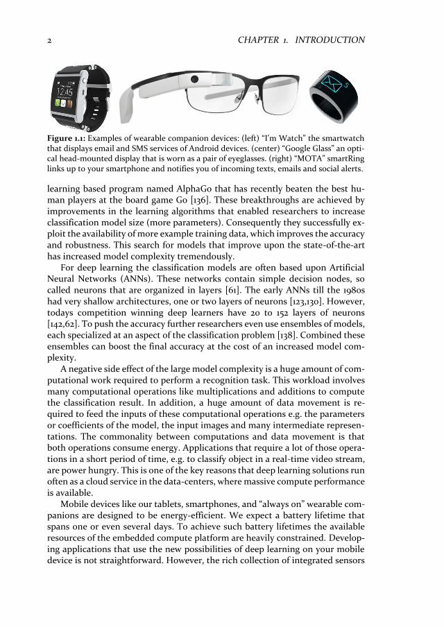
Nowadays digital technology is interwoven into many aspects of our daily lives. For example, think of the omnipresence of personal devices such as smartphones, tablet computers, digital cameras, and televisions that guide our decisions and instantly connect us to the internet. From another perspective es-timate your daily usage of services such as e-mail, online encyclopedias, on-line shopping, and digital music. More and more we are accessing services through our smartphones; this is reflected by the number of mobile smartphone sub-scriptions that globally grew by 18% in 2016 to reach 3.9 billion1. This trend will extend from smartphone to smart devices, a class of wearable companion devices that integrates digital services deeply into our daily life. Figure 1.1 depicts a few examples devices such as, smartwatches, smart glasses [140], and in the extreme a smart ring.
The new challenge is to make these so called “smart devices” really smart. Checking e-mail or posting photos on social media are just the first features. The real smart features use integrated sensors like cameras to identify objects in im-ages. Or with a microphone instead of a camera that directly transcribes speech into text. Such features are already successfully used in data-centers (providing cloud services for Google and Facebook) to handle image search queries. Cur-rently, these tasks are solved by Machine Learning techniques that extract and recognize patterns from huge loads of raw data. Increasingly, these recognition applications make use of a class of techniques called Deep Learning.
Probably you have heard or read about deep learning; it is a lot in the news since big companies like Google, Facebook, and Microsoft are acquiring start-ups with expertise in this field. In the last few years, deep learning made major advances e.g., it has beaten many records in image recognition [79,30,49], and speech recognition [66,127]. Most striking is the fact that in some cases these techniques achieved superhuman (better than human) accuracy in solving diffi-cult pattern recognition problems [30,25]. A well know example is the deep
1 Source: Ericsson Mobility Report Nov 2016.
CHAPTER
2 CHAPTER 1. INTRODUCTION
learning based program named AlphaGo that has recently beaten the best hu-man players at the board game Go [136]. These breakthroughs are achieved by improvements in the learning algorithms that enabled researchers to increase classification model size (more parameters). Consequently they successfully ex-ploit the availability of more example training data, which improves the accuracy and robustness. This search for models that improve upon the state-of-the-art has increased model complexity tremendously.
For deep learning the classification models are often based upon Artificial Neural Networks (ANNs). These networks contain simple decision nodes, so called neurons that are organized in layers [61]. The early ANNs till the 1980s had very shallow architectures, one or two layers of neurons [123,130]. However, todays competition winning deep learners have 20 to 152 layers of neurons [142,62]. To push the accuracy further researchers even use ensembles of models, each specialized at an aspect of the classification problem [138]. Combined these ensembles can boost the final accuracy at the cost of an increased model com-plexity.
A negative side effect of the large model complexity is a huge amount of com-putational work required to perform a recognition task. This workload involves many computational operations like multiplications and additions to compute the classification result. In addition, a huge amount of data movement is re-quired to feed the inputs of these computational operations e.g. the parameters or coefficients of the model, the input images and many intermediate represen-tations. The commonality between computations and data movement is that both operations consume energy. Applications that require a lot of those opera-tions in a short period of time, e.g. to classify object in a real-time video stream, are power hungry. This is one of the key reasons that deep learning solutions run often as a cloud service in the data-centers, where massive compute performance is available.
Mobile devices like our tablets, smartphones, and “always on” wearable com-panions are designed to be energy-efficient. We expect a battery lifetime that spans one or even several days. To achieve such battery lifetimes the available resources of the embedded compute platform are heavily constrained. Develop-ing applications that use the new possibilities of deep learning on your mobile device is not straightforward. However, the rich collection of integrated sensors
Figure 1.1: Examples of wearable companion devices: (left) “I’m Watch” the smartwatch that displays email and SMS services of Android devices. (center) “Google Glass” an opti-cal head-mounted display that is worn as a pair of eyeglasses. (right) “MOTA” smartRing links up to your smartphone and notifies you of incoming texts, emails and social alerts.

1.1. NEURAL NETWORKS FOR CLASSIFICATION 3
in mobile and wearable devices make them the best target for state-of-the-art classifier applications. To bridge the compute energy gap between deep learning algorithm requirements and the capabilities of modern embedded platforms the energy efficiency must be improved. The goal of this thesis is therefore to sub-stantially improve the efficiency of deep convolutional networks. These convolu-tional nets are specialized in visual data processing and recently very popular in machine learning. This chapter will introduce Neural networks (Section 1.1), and explain their evolution into Deep Convolutional Networks (Section 1.2). Next, the trends in Deep Learning research are outlined (Section 1.3), and the problem statement is discussed in detail (Section 1.4). Finally, the main contributions and chapter outline are presented in Section 1.5 and Section 1.6 respectively.
1.1 Neural networks for classification
Most work on artificial neural networks has been motivated by the observation that the human brain computes in an entirely different way than digital comput-ers do. Instead of performing complex tasks sequentially, the brain solves com-plex problems in a distributed and highly parallel approach with simple unreliable operations performed by units known as neurons. Although its pro-cessing is very different the brain is very successful, and reliable in processing complex tasks. Consider for example vision, the brain can process the visual in-formation of the environment around us in a split second. It extracts the context of a scene, warns you for threatening situations, and directly remembers the faces of the people involved. This task requires distinguishing foreground from background, recognizing objects presented in a wide range of orientations, and accurately interpreting spatial cues. The human brain performs such tasks with great ease and compared to modern compute platforms it requires a very modest power budget.
This section will introduce the basic processing elements of neural networks, their interconnections, and their ability to classify patterns. These aspects are addressed without focusing on their capability to learn by adapting their param-eters. Training is one of the key features of neural nets, which will be further discussed in Chapter 3 and 4.
1.1.1 Modeling a neuron
The fundamental processing elements in neural networks are their neurons. The block diagram in Figure 1.2 illustrates the model of a neuron. It forms the basic element for a large family of neural networks that is studied in the further chap-ters of this thesis. A simple form of this model is already developed in 1943 by the pioneering work of McCulloch and Pitts [94]. There are basically three ele-ments in this neuron model:

4 CHAPTER 1. INTRODUCTION
1. A set of connecting input links xj or synapses, each characterized by a weight or strength wj. The weights model the synaptic efficiency of bio-logical connections, unlike the synapses in the human brain the weights of an artificial neuron cover a range that includes negative as well as positive values.
2. A summing junction or adder for summing the input signals, weighted by the respective synaptic strengths.
3. An activation function for limiting the range of the output signal to some finite value. In addition, this function can add non-linear behavior to neural networks.
The artificial neuron of Figure 1.2 also includes a bias value, denoted by b. Depending on whether the bias is positive or negative it can increase or lower the net input of the activation function. The neuron model can be mathemati-cally described by using a simple pair of equations:
𝑝𝑖 = 𝑏𝑖 +∑𝑤𝑖𝑗 𝑥𝑗
𝐾−1
𝑗=0
(1.1)
𝑦𝑖 = φ(𝑝𝑖) (1.2)
The neuron potential pi is computed by the weighted sum of the inputs xj; wi0, wi1, …, wiK-1, are the respective synaptic weights of neuron i. The activation po-tential has an external offset bias bi. Note that the bias also could be encoded as one of the weights, e.g. wi0 = bi, and x0 = 1. The activation function φ() transforms the neuron potential into an output value. Different activation functions are dis-cussed below.
Assume that the artificial neuron model is used as digit detector e.g., for the number one as displayed on the left side of Figure 1.2. In this scenario the poten-tial should be high if the number one is applied, for all other patterns it should be low. This is achieved when inputs connected to black pixels have positive weights (excitatory inputs) and other positions negative weights (inhibitory in-puts). This ensures that for digits with a significant amount of overlap, e.g. the
Figure 1.2: A basic nonlinear model of a neuron with an example input pattern.
∑=p
w0
w1
w2
x0
x1
x2
xK-1
Bias
b
Synaptic weigths
Summing junction
φ(p)
Output
y0-1
0 0
0 0
0 1
0 0
0 0
0 0
1 0
1 0
1 0
1 0
0
0
0
0
0
0 1
0 0
1 1
0 0
0
0
Activation function
Example input vector
wK-1
Perceptron
1.1. NEURAL NETWORKS FOR CLASSIFICATION 5
number two, the inhibitory inputs mitigate the overlapping positions resulting in a reduced potential.
Types of activation functions
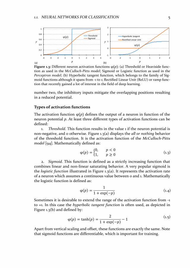
The activation function φ(p) defines the output of a neuron in function of the neuron potential p. At least three different types of activation functions can be defined:
1. Threshold. This function results in the value 1 if the neuron potential is non-negative, and 0 otherwise. Figure 1.3(a) displays the all or nothing behavior of the threshold function. It is the activation function of the McCulloch-Pitts model [94]. Mathematically defined as:
φ(𝑝) = {0, 𝑝 < 01, 𝑝 ≥ 0
(1.3)
2. Sigmoid. This function is defined as a strictly increasing function that combines linear and non-linear saturating behavior. A very popular sigmoid is the logistic function illustrated in Figure 1.3(a). It represents the activation rate of a neuron which assumes a continuous value between 0 and 1. Mathematically the logistic function is defined as:
φ(𝑝) =1
1 + exp(−𝑝) (1.4)
Sometimes it is desirable to extend the range of the activation function from -1 to +1. In this case the hyperbolic tangent function is often used, as depicted in Figure 1.3(b) and defined by:
φ(𝑝) = tanh(𝑝) =2
1 + exp(−𝑝)− 1
(1.5)
Apart from vertical scaling and offset, these functions are exactly the same. Note that sigmoid functions are differentiable, which is important for training.
0
0.2
0.4
0.6
0.8
1
-4 -3 -2 -1 0 1 2 3 4
y
p
ThresholdSigmoid
φ(p)
(a)
-1
0
1
2
3
-3 -2 -1 0 1 2 3
y
p
Hyperbolic tangent
Rectified Linear Unit
φ(p)
(b)
Figure 1.3: Different neuron activation functions φ(p): (a) Threshold or Heaviside func-tion as used in the McCulloch-Pitts model; Sigmoid or Logistic function as used in the Perceptron model; (b) Hyperbolic tangent function, which belongs to the family of Sig-moid functions although it spans from -1 to 1; Rectified Linear Unit (ReLU) or ramp func-tion that recently gained a lot of interest in the field of deep learning.
6 CHAPTER 1. INTRODUCTION
3. Rectifier. A neuron model that employs a rectifier function is also called a Rectified Linear Unit (ReLU). This function is, as of 2015 the most popular acti-vation function for deep neural networks, it performs very well for deeper net-works [79]. Figure 1.3(b) shows the ReLU activation function that is defined as:
φ(𝑝) = max (0, 𝑝) (1.6)
A ReLUs is not fully differentiable, p below and on 0 have slope 0, above gives 1.
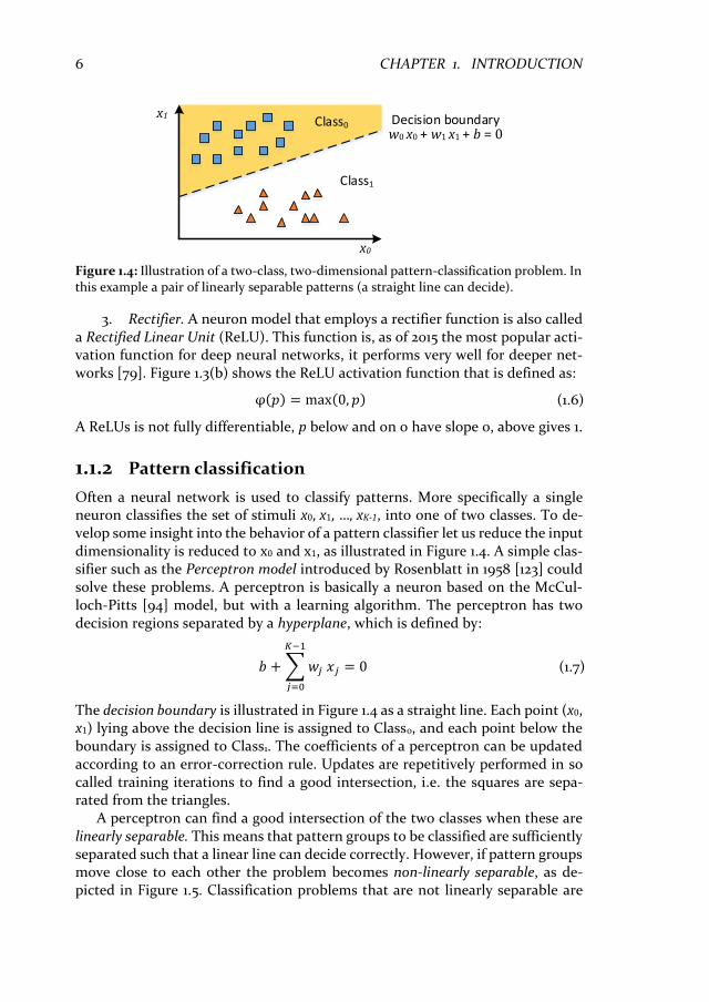
1.1.2 Pattern classification
Often a neural network is used to classify patterns. More specifically a single neuron classifies the set of stimuli x0, x1, …, xK-1, into one of two classes. To de-velop some insight into the behavior of a pattern classifier let us reduce the input dimensionality is reduced to x0 and x1, as illustrated in Figure 1.4. A simple clas-sifier such as the Perceptron model introduced by Rosenblatt in 1958 [123] could solve these problems. A perceptron is basically a neuron based on the McCul-loch-Pitts [94] model, but with a learning algorithm. The perceptron has two decision regions separated by a hyperplane, which is defined by:
𝑏 +∑𝑤𝑗 𝑥𝑗
𝐾−1
𝑗=0
= 0 (1.7)
The decision boundary is illustrated in Figure 1.4 as a straight line. Each point (x0, x1) lying above the decision line is assigned to Class0, and each point below the boundary is assigned to Class1. The coefficients of a perceptron can be updated according to an error-correction rule. Updates are repetitively performed in so called training iterations to find a good intersection, i.e. the squares are sepa-rated from the triangles.
A perceptron can find a good intersection of the two classes when these are linearly separable. This means that pattern groups to be classified are sufficiently separated such that a linear line can decide correctly. However, if pattern groups move close to each other the problem becomes non-linearly separable, as de-picted in Figure 1.5. Classification problems that are not linearly separable are
Figure 1.4: Illustration of a two-class, two-dimensional pattern-classification problem. In this example a pair of linearly separable patterns (a straight line can decide).
x0
x1Class0
Class1
Decision boundaryw0 x0 + w1 x1 + b = 0

1.1. NEURAL NETWORKS FOR CLASSIFICATION 7
beyond the capability of a single neuron or perceptron. This is a severe limitation of the perceptron model that prevents it from making more complex classifica-tions; e.g., it cannot even solve a binary parity problem like a simple XOR func-tion. This made that artificial neurons fell in despair from the 1960s till the mid-1980s.
In finalizing the introduction of artificial neurons or the perceptron we con-clude that the model is an elegant approach to classify linearly separable pat-terns. However for more complicated patterns like non-linearly separable ones this model is too restricted. Although these limitations perceptron’s have proven to be very useful for the development of machine learning. In fact they are now-adays still used as internal building block for the successful deep learning tech-niques. The next section will show how to extend the learning and classification capabilities of perceptron’s.
1.1.3 Multilayer perceptron’s
To be able to classify more difficult not linearly separable problems a two-step approach is required. Firstly, the input signals should be transformed into a new representation into so called features. This new representation should separate the classes further apart from each other, which makes it easier to separate the classes. Secondly, a new classifier should use the new representation as input to solve the classification problem. An analogy of this two-step approach is to com-pare it to how you read a sentence. You do not care about each individual char-acter. Firstly, these characters are classified into words. Secondly, you parse the words into a sentence with his own meaning. If you would lose the ability to recognize words, it would become much more difficult to understand the con-tent of a sentence.
Learning representations is exactly what a multilayer perceptron performs. As depicted in Figure 1.6, the multilayer network has a hidden layer (neuron h0, h1, h2) between input and output. The hidden neurons act as feature detectors; they perform a non-linear transformation on the inputs. During the learning process these hidden neurons discover the features that characterize the training data. The formation of this extra feature space distinguishes the multilayer perceptron from a single perceptron. The illustrated multilayer perceptron in Figure 1.6 re-veals that the network is a directed graph, where each layer is fully connected to
Figure 1.5: Illustration of a two-dimensional pair of non-linearly separable patterns. x0
x1Class0
Class1
Non-linear decision boundary
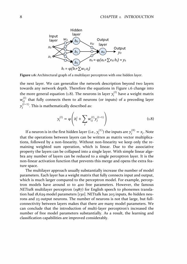
8 CHAPTER 1. INTRODUCTION
the next layer. We can generalize the network description beyond two layers towards any network depth. Therefore the equations in Figure 1.6 change into
the more general equation (1.8). The neurons in layer 𝑦𝑖(𝑙)
have a weight matrix
𝑤𝑖𝑗(𝑙)
that fully connects them to all neurons (or inputs) of a preceding layer
𝑦𝑗(𝑙−1)
. This is mathematically described as:
𝑦𝑖(𝑙)= φ(𝑏𝑖
𝑙 +∑𝑤𝑖𝑗(𝑙)𝑦𝑗(𝑙−1)
𝑗
) (1.8)
If a neuron is in the first hidden layer (i.e., 𝑦𝑖(1)
) the inputs are 𝑦𝑗(0)= 𝑥𝑗 . Note
that the operations between layers can be written as matrix vector multiplica-tions, followed by a non-linearity. Without non-linearity we keep only the re-maining weighted sum operation, which is linear. Due to the associative property the layers can be collapsed into a single layer. With simple linear alge-bra any number of layers can be reduced to a single perceptron layer. It is the non-linear activation function that prevents this merge and opens the extra fea-ture space.
The multilayer approach usually substantially increase the number of model parameters. Each layer has a weight matrix that fully connects input and output, which is much larger compared to the perceptron model. For example, percep-tron models have around 10 to 400 free parameters. However, the famous NETtalk multilayer perceptron (1987) for English speech to phonemes transla-tion had 18,629 model parameters [130]. NETtalk has 203 inputs, 80 hidden neu-rons and 23 output neurons. The number of neurons is not that large, but full-connectivity between layers makes that there are many model parameters. We can conclude that the introduction of multi-layer perceptron’s increased the number of free model parameters substantially. As a result, the learning and classification capabilities are improved considerably.
Figure 1.6: Architectural graph of a multilayer perceptron with one hidden layer.
h0
h1
h2
x0
x1
Hidden layer
Outputy0n0
Outputlayer
hi = φ(bi+∑wij xj)
nk = φ(ak+∑vkl hl) = yk
Input layer wij
vkl

1.1. NEURAL NETWORKS FOR CLASSIFICATION 9
1.1.4 Generalization issues
One of the key properties of (multilayer) perceptron’s is the ability to train them with a labelled dataset. This is called Supervised Learning or learning with a teacher. It requires a set of input examples with corresponding output labels. The learning algorithm iterates over these samples and corrects the errors on the outputs by adjusting the weights in the network. An efficient algorithm for train-ing is error-backpropagation. It adjusts the weights by using the gradient infor-mation of errors. Computing the error gradients is done efficiently by propagating back the errors through the networks. Chapter 2 presents more de-tails regarding this learning process.
Since the mid-1980s the back-propagation algorithm caused revived interest into artificial neural networks [125]. Many researchers where using neural net-works for pattern classification problems; non-linearly separable problems seemed no problem for multilayer perceptron’s. They used many training exam-ples and hoped that the designed neural net would generalize well. A network generalizes well if the input-output mapping is correct or nearly correct for test data that is not used for training the network. Generalization represents how the network would perform in a real-world environment where it is continually ex-posed to new data.
A neural network that is designed to generalize well will produce a correct input-output mapping even when input samples are slightly different from the ones used for training. Generalization is mainly influenced by three factors:
1. The size of the training set and how representative it is for the problem. 2. The architecture of the neural network, or training method (regulariza-
tion methods can reduce overfitting). 3. The complexity of the problem at hand.
Figure 1.7: Examples of classifier decision spaces and generalization: (a) Under fitting, a linear classifier cannot distinguish the two classes correctly, it has not enough parame-ters; (b) A small multilayer perceptron. Not all training samples are classified correctly. However, it shows good generalization, most new samples are expected to be classified correctly; (c) Over fitting, classifier is too complex. It fits “noise” in the training data. All training samples are classified correctly, but new samples will probably introduce errors.
x0
x1
Class0
Class1
x0
x1
Class0
Class1
x0
Class0
Class1x1
Under fitting Good generalization Over fitting
(a) (b) (c)

10 CHAPTER 1. INTRODUCTION
Figure 1.7 illustrates how these three aspects influence generalization. Under fit-ting is depicted in Figure 1.7(a), the classifier is too simplistic (too rigid), it can-not capture salient patterns in the data. Although it makes errors on the training data, for the common case it will not perform much worse on new test data. The distribution of triangles suggest that new triangles probably will appear in the top right (yellow) part of the decision space. Although the model suffers from under fitting, we conclude that it generalizes reasonably. Figure 1.7(b) illustrates a classifier that has a good fit on the data. Not all samples in the training set are classified correctly, but it is likely that the two errors are outliers that will not appear again. Over fitting is demonstrated in Figure 1.7(c), the classifier is too complex (too flexible). It clearly fits on the “noise” in the training data. All train-ing patterns are classified correctly, but this includes patterns that will not re-appear. If this complex classifier is used in a real-world environment with new samples it will probably make many errors.
Especially for shallow networks with many parameters, it is difficult obtain a good generalization. So called shallow networks have one or few, but large hid-den layers. To find single transformations of the inputs into classifications by using many parameters is difficult. With less parameters the network is forced to make abstractions of the problem, which often helps generalization. The gen-eralization issues show that more difficult problems are not automatically solved by increasing the number of neurons in the hidden layer. Simply increasing the number of neurons (adding model complexity) is not directly the solution to solve more difficult problems.
1.2 Deep networks for computer vision
One of the more complex pattern classification problems is visual object recog-nition. Tasks that humans solve relatively simply can be very challenging for al-gorithms. Think of detecting a familiar face, reading road signs, or interpretation of hand written characters. Figure 1.8, illustrates that such images are con-structed by pixels with a corresponding intensity value. In a digital system these
86 90 79 83 77 68
85 222
58 88
232 240 199 92
63 57 240 79
68 71 63 211 74 85
91 87
195 46
197 65 58 46
64 55 35 38
Figure 1.8: Examples of visual object recognition tasks: Detecting a familiar face; reading a speed sign; Interpret hand written characters. Easy tasks for humans, however for a computer it is an array of pixel values. It results in a high-dimensional input vector. Would you recognize the number 7 in the example matrix on the right hand side?

1.2. DEEP NETWORKS FOR COMPUTER VISION 11
images are arrays of pixel intensity values. It is quite hard for us humans to ex-tract the number 7 from the array by only looking at the numeric values in the array. Especially if you take into account that all pixel values will change when external light conditions alter. This subsection briefly discuss the techniques used to improve neural net architectures to perform well on visual data. Enforc-ing architecture constraints as shown in Section 1.2.1 is a successful technique to improve generalization for image recognition tasks. These architectural con-straints resulted in networks that stack feature hierarchies, see 1.2.2. It is the ba-sis of the successful Convolutional Networks (ConvNets). More information on this topic will be given in Chapter 2.
1.2.1 Building prior information in neural net architectures
When a neural network is used as face detector it should learn to separate a face from background. E.g., an input patch of 20x20 pixels can be used as input (input retina), which should be classified as face or background. The high dimension-ality of the input vector (400 input values) makes it very challenging to train a multilayer perceptron correctly with a good generalization. A very successful ap-proach to cope with the difficulties of high dimensional input data is: Incorpo-rate prior knowledge about the problem into the model parameters. This reduces the flexibility of the classifier (prevent over fitting). In addition, it forces the re-maining parameters to learn only useful correlations in the training data.
20 by 20 pixels
Input vector
Receptive fields
Hidden layer
Output layer
Figure 1.9: Example of Rowely’s constrained multilayer perceptron. Prior knowledge is embedded in the network e.g., receptive fields specialized at detecting eyes, or mouth shapes. Weight freedom is limited to enforce important features and prevent overfitting.

12 CHAPTER 1. INTRODUCTION
Receptive fields
Figure 1.9 depicts a good example of a network architecture that reduces con-nectivity and incorporates prior knowledge for face detection [124]. Instead of fully connecting the high dimensional input to all neurons in the hidden layer; the hidden layer has three types of specialized receptive fields. Receptive fields are input regions that are connected to a neuron, e.g. the red 10x10 input boxes in Figure 1.9 show a limitation on the connected inputs. Each of these types is chosen to enforce hidden neurons to detect local features that are important for face detection. In particular, square shaped receptive fields might detect features such as individual eyes, the nose, or corners of the mouth. Stripe shaped recep-tive fields can detect mouths or a pair of eyes. The constrained network archi-tecture reduces the number of free model parameters to 1,453 compared to 10,427 for a fully connected hidden layer. At the time of introduction (1998) this con-strained network architecture significantly improved upon the state-of-the-art for face detection.
Weight sharing
A second additional measure that is used to build prior information into neural networks is weight-sharing. Weight sharing constrains the parameter freedom by enforcing the same weights for multiple neurons. This is better demonstrated by the partially connected network depicted in Figure 1.10. The top four inputs belong to the receptive field of hidden neuron 1, and so on for the other hidden neurons in the network. To satisfy the weight-sharing constraint, the same set of synaptic weights is used for each neuron in the hidden layer of the network. The potential of neuron i is mathematically expressed as:
𝑝𝑖 = 𝑏 +∑𝑥𝑖+𝑘𝑤𝑘
𝐾−1
𝑘=0
(1.9)
The weights wk are used on shifted input positions similar to a convolutional sum. Compared to receptive fields, weight sharing reduces the number of free
x1
x2
x3
x4
x5
x6
x7
y1
y2
Hidden layerOutput layer
Input layer
Figure 1.10: Illustration of weight sharing combined with receptive fields. All four hidden neurons share the same set of weights for their four synaptic inputs.

1.2. DEEP NETWORKS FOR COMPUTER VISION 13
parameters even further. The hidden layer is forced to learn only the most im-portant local features. An additional side effect of sharing with a convolutional sum is translation/position invariance. The concept of weight sharing with re-ceptive fields can be easily extended to 2d input images. Especially for vision tasks position invariance of features can be important. Think of edge detection algorithms, it does not matter where the edges occur to classify them as edges. Local position invariant features like edges are important clues for the classifi-cation of an object. In ConvNets a combination of both reducing connectiv-ity/receptive fields and weight sharing is used. Chapter 2 will elaborate more on this topic and give a detailed motivation why local features are important for vision tasks.
1.2.2 Feature hierarchies
One of the problems with two layer perceptron networks is that the hidden neu-rons interact with each other globally. For complicated problems this interaction makes it difficult to improve the classifier for certain input patterns without worsening it for others. With multiple hidden layers, the process of learning the best features becomes more manageable. Classical model based image recogni-tion pipelines apply the same partition of classification into several stacked steps. These models separate a recognition task into feature extraction and clas-sification, as illustrated by Figure 1.11.
1. Feature extraction can involve multiple successive steps such as pre-pro-cessing and extraction of features. This step makes it easier to classify the data, and increases the likelihood of correct classification by removal of irrelevant var-iations. For example, illumination normalization, and translating to edges or gradients which are not much affected by the illumination. Examples of ad-vanced model based feature extractors are: SIFT [91]; SURF [4]; and HOG [38].
2. Classification is performed on the feature vector that is carefully de-signed to reduce the amount of data, and amplify only important aspects of the recognition task. The classification task can be performed by a simple classifier model, e.g., a Perceptron, k-Nearest Neighbour (k-NN), or a Support Vector Ma-chine (SVM).
The very successful idea of solving classification problems in a hierarchical approach is also applied to neural networks. These can also exploit the property that many signals in nature are composed of hierarchies, in which higher-level features are obtained by composing lower-level ones. In images, local combina-tions of edges form motifs that are arranged into parts, and parts form objects.
Invariant feature extractor
Classification model
Input pattern X
Feature vector
Y
Outputs
Figure 1.11: Block diagram of a classical two step object recognition system.

14 CHAPTER 1. INTRODUCTION
In speech and text similar hierarchies can be observed: from sounds to phones, phonemes, syllables, words and sentences. These hierarchal part-whole relation-ships apply to almost every object recognition task.
Section 1.2.1 shows how prior information is embedded into a network archi-tecture. By stacking layers crafted to detect features from the corresponding hi-erarchical level, one obtains a classifier that is much easier to train, and has greatly improved generalization properties. Each hidden layer can perform a non-linear transformation of the previous layer, so a deep network (multiple hid-den layers) can compute more complex features of the input. In the case of vision tasks deeper networks learn part-whole decompositions as described above. For instance, the first layer groups pixels together to detect edges. A second layer might group together the edges to detect longer contours. Even deeper layers can group together these contours and detect parts of objects. Learning such deep feature hierarchies by training many stacked layers is what the term Deep Learning refers to.
1.3 Trends in deep neural network development
The depth increase of classifiers by stacking many layers is a key differentiator from the earlier shallow models. It resulted in remarkable improvements in clas-sifier accuracy. For example, new deep networks are breaking records in image recognition [79,30,49], and speech recognition [66,127]. In addition, they are very successful in other domains e.g. drug discovery, as demonstrated by the winning entry in the Kaggle2 competition to predict useful drug candidates for pharma company Merck [93]. Nowadays on many tasks deep networks achieve near-human accuracy levels e.g., Face detection [143]. In extreme cases these deep nets deliver superhuman accuracy, as demonstrated by [25,63].
The recently introduced machine learning models that challenge human ac-curacy levels have a long history. From the simple models of the 1940s they evolved into the powerful classifiers of today. This evolution is not only reflected by their accuracy scores or the difficulty of the problems they solve. The detec-tion scores are a result of many model parameters and huge amounts of training data used to tune these parameters. This section takes a closer look at the his-torical trends in deep neural network development. Throughout this section, a set of 30 popular neural network publications is used as historical data3, each representative for the state-of-the-art at their year of publication.
2 The Merck Molecular Activity Challenge on www.kaggle.com 3 Neural network articles used for trend analysis: [13,24-31,51,59,63,64,74,77-82,88,111,112,114,115,121,
122,127,128,132] [88,114,121,77,78,13,115,79,80,51] [127,112,81,63,64,111,26,27,28,29] [24,30,82,74,25,31,122,132,128,59]

1.3. TRENDS IN DEEP NEURAL NETWORK DEVELOPMENT 15
1.3.1 Model capacity
In Figure 1.12, the model size of classifier networks published during the last 70 years is illustrated. Model size is given as the number of trainable model param-eters, i.e. the number of weights. In addition, the computational workload de-fined as the number of Multiply Accumulate operations required for a single classification is plotted. This data shows an important observation:
Both model size and computational workload have grown immensely over time, especially since 2008 there was an acceleration of the already impressive growth rate. The model growth is reflected by an increasing complexity of the classification tasks solved by neural networks. The old perceptron’s of the 1950s learned linearly separable patterns like simple lines and planes [123]. However competition winners of today’s ImageNet summarize the content of a million images, they recognize 1000 different classes of complex objects such as ham-mers, or bikes, ants, etcetera [126]. The huge complexity of these tasks is repre-sented by the data set size, which has grown tremendously. To absorb this enormous amount of training data the number of model parameters in neural networks exploded. The dotted exponential trend lines in Figure 1.12 reveal the immense growth of model parameters and computational work. Let’s have a closer look at the breakthroughs that enabled the exponential growth rate in model capacity.
The first single layer networks of the 1940s to 1950s had up to 400 model parameters. During the 1980s the error back-propagation algorithm helped to
Figure 1.12: Historical data on 30 neural networks3 showing the explosive scaling for the number of model parameters, and involved computational workload. Multiply Accumu-late (Macc) are the used measure for computational workload.
10
100
1000
10000
100000
1000000
10000000
100000000
1E+09
1E+10
1E+11
1940 1950 1960 1970 1980 1990 2000 2010 2020
Year of introduction
Model parameters
Compute Workload [Macc]
Expon. (Model parameters)
Expon. (Compute Workload [Macc])

16 CHAPTER 1. INTRODUCTION
train larger multi-layer networks like NETtalk with 18.000 parameters [130]. Around 2000 techniques as receptive fields and weight sharing evaluated into the Convolutional Networks of Yann LeCun [84]. The Convolutional nets pushed the number of model parameters over 90.000 while maintaining excellent gen-eralization [85]. In addition, Convolutional Nets increased the depth of classifier models from two layer models to 4-7 layers. Figure 1.13, illustrates the network depth increase caused by the introduction of Convolutional Networks. From 2006 onwards weight regularization techniques enabled regular non weight sharing networks to scale in depth to 4-7 layers [67,68]. These nets, so called Deep Belief Networks (DBN), increased the model size to almost 4 million pa-rameters.
Around 2008 the availability Graphics Processing Units (GPUs) for general purpose computing improved the computational abilities of machine learning scientists. The use of GPUs resulted in huge networks; e.g., DBNs with 100 mil-lion parameters are successfully trained [118]. In addition to GPUs, the introduc-tion of huge data sets in 2012 like the 1 million images of the ImageNet competition in 2012 [126] pushed the state-of-the-art Convolutional Networks to 60 million parameters divided over 11 layers [79]. This 60 million parameter net-work named “AlexNet” won the competition by a large margin over other ap-proaches. Due to the success of AlexNet many research groups now contribute to the development of large classifier models. Nowadays the largest Convolu-tional Nets such as VGG have 280 million parameters [138]. In the extreme, huge DBNs with 11 billion parameters are trained by GPU clusters [32]. These examples
Figure 1.13: Depth increase of neural networks over the last 70 years on a linear scale. Note that recently introduced residual networks have a depth of 152 layers [58] and be-yond.
0
5
10
15
20
25
30
1940 1950 1960 1970 1980 1990 2000 2010 2020
Net
wo
rk d
epth
N la
yers
Year of introduction
Network Layers

1.3. TRENDS IN DEEP NEURAL NETWORK DEVELOPMENT 17
demonstrate the tremendous growth in classifier model size over time, and it is not expected that this growth will stop any soon.
1.3.2 Computational work
The computational requirements of deep neural nets have grown even faster than the number of model parameters. This claim is supported by the exponen-tial trend lines in Figure 1.12. For the early neural networks computational work-load scaled with the number of trainable model parameters. For example, each layer of neurons was fully connected, it required as many multiply accumulate operations as the number of weights in the network. However, the introduction of weight sharing since 1990 made that weights are reused for multiple compute operations. As a result, the number of compute operations grew even faster than the number of model parameters.
The role of computing platforms
To train increasingly larger nets with the impressive pace as presented in Figure 1.12 the machine learning community is driven by huge developments in compu-ting platforms. Very important are the developments that enabled transistor scaling; e.g. Moore’s Law [96] is a fundamental driver of computing over the past 40 years. In more detail, chip manufacturing facilities have been able to develop every 18 months new technology generations that double the number of transis-tors on a single chip. However, more transistors does not give any benefits by itself. It is the computer architecture industry that utilizes these transistors in new microprocessor designs. Computer architecture (in particular the ISA, In-struction Set Architecture of a processor) provides the abstractions that make these transistors accessible to compilers, programming languages, application developers, and machine learners.
Computer architecture harvested the exponentially increasing number of transistors to deliver an almost similar rate of performance improvement for mi-croprocessors. The huge performance increase helped machine learners to build and train large neural networks. Nevertheless there are fundamental challenges associated with the development of new process technologies and integrating an exponential increasing number of transistors on a chip. One of the main chal-lenges when doubling the number of transistors is powering them without melt-ing the chip. During the last 15 years power consumption has become a huge problem in the field of computer architecture.
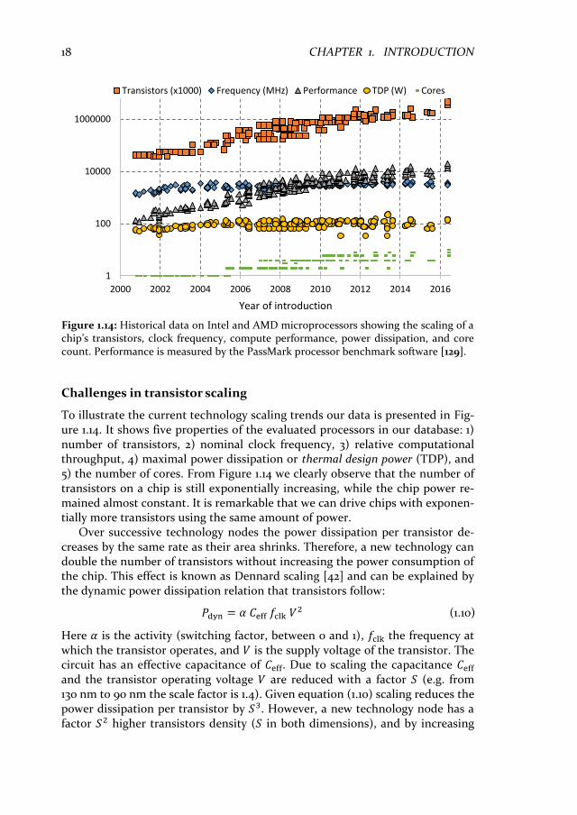
To quantify the power problem and look into possible directions for the com-ing decade we analyzed recent trends for desktop grade microprocessors. In this study data from 218 Intel and AMD processors is used by combining data from Intel’s ARK database [72], which is extended with information from Wikipedia [149,148]. In addition, the relative computational throughput is added, which is measured by the PassMark processor benchmark software [139].
18 CHAPTER 1. INTRODUCTION
Challenges in transistor scaling
To illustrate the current technology scaling trends our data is presented in Fig-ure 1.14. It shows five properties of the evaluated processors in our database: 1) number of transistors, 2) nominal clock frequency, 3) relative computational throughput, 4) maximal power dissipation or thermal design power (TDP), and 5) the number of cores. From Figure 1.14 we clearly observe that the number of transistors on a chip is still exponentially increasing, while the chip power re-mained almost constant. It is remarkable that we can drive chips with exponen-tially more transistors using the same amount of power.
Over successive technology nodes the power dissipation per transistor de-creases by the same rate as their area shrinks. Therefore, a new technology can double the number of transistors without increasing the power consumption of the chip. This effect is known as Dennard scaling [42] and can be explained by the dynamic power dissipation relation that transistors follow:
𝑃dyn = 𝛼 𝐶eff 𝑓clk 𝑉2 (1.10)
Here 𝛼 is the activity (switching factor, between 0 and 1), 𝑓clk the frequency at which the transistor operates, and 𝑉 is the supply voltage of the transistor. The circuit has an effective capacitance of 𝐶eff. Due to scaling the capacitance 𝐶eff and the transistor operating voltage 𝑉 are reduced with a factor 𝑆 (e.g. from 130 nm to 90 nm the scale factor is 1.4). Given equation (1.10) scaling reduces the power dissipation per transistor by 𝑆3. However, a new technology node has a factor 𝑆2 higher transistors density (𝑆 in both dimensions), and by increasing
Figure 1.14: Historical data on Intel and AMD microprocessors showing the scaling of a chip’s transistors, clock frequency, compute performance, power dissipation, and core count. Performance is measured by the PassMark processor benchmark software [129].
1
100
10000
1000000
2000 2002 2004 2006 2008 2010 2012 2014 2016
Year of introduction
Transistors (x1000) Frequency (MHz) Performance TDP (W) Cores

1.3. TRENDS IN DEEP NEURAL NETWORK DEVELOPMENT 19
𝑓clk.by a factor 𝑆 the chip power remains constant. Note that the potential per-formance of the new technology went up by a factor 𝑆3 (faster and more transi-tors).
The bad news is that since 2005, at the 90 nm node, the rate of supply voltage scaling dramatically slowed down due to limits in threshold voltage scaling. As a result Dennard scaling stopped from that point onwards [42]. The number of transistors on a chip continued to grow with the historical rate, while the power per transistor is not decreasing at the same rate. This quickly results in power dissipation issues, especially since 100 Watt per chip/die is about the limit if no excessive cooling is applied. For embedded devices these limits are even lower e.g., 10 Watt for Tablets, 1 Watt for Smartphones, and 0.1 Watt for wearables.
Computer architecture challenges
The first step to prevent excessive power consumption is to stop increasing the clock frequency 𝑓clk. Figure 1.14 shows that since 2005 clock frequency stopped increasing and it leveled around 3.5 GHz. To maintain improvements in compu-tational throughput and utilize the extra transistors of new technology nodes multicore architectures are introduced. Instead of more complex and faster sin-gle-cores, multiple simpler and lower frequency cores are integrated on a die. By exploiting parallelism in the applications multicore processors try to overcome the trends in transistor level scaling [134].
If we study equation (1.10) more closely we observe a factor 𝑆2 power increase because Dennard scaling stopped. Not increasing the clock frequency reduces this problem to a factor 𝑆 power increase. This reveals another challenge for the near future; it might not be possible to turn on and utilize all the transistors that scaling provides due to power limitations. In addition, it is often very difficult to exploit enough application parallelism to utilize all cores in a multicore archi-tecture. This second utilization problem automatically reduces the number of transistors that are turned on. Both problems make that in current technology nodes a growing portion of transistors is underutilized. A popular term for these chip portions that are underutilized is ‘dark silicon’.
The implications of this growing portion of dark silicon pose great challenges for computer architecture. As a result it will become more difficult to increase computational performance over time. A recent exhaustive and comprehensive quantitative study by Esmaeilzadeh et al. [48] estimated the impact of dark sili-con on the performance of processors. Under optimistic assumptions they pre-dict that performance will increase by 7.9x over a period of ten years, resulting in a 23-fold gap w.r.t. the historic doubled performance per generation. If their predictions are correct the microprocessor performance increase per generation will dramatically slow down. As a result, this process will slow down develop-ments in the application domains that benefit from the historic performance in-crease. Among these applications the huge and deep neural networks will face this problem. However, the work of Esmaeilzadeh et al. is a prediction, with our new dataset we can quantify the accuracy of their prediction.

20 CHAPTER 1. INTRODUCTION
The dark silicon performance prediction of Esmaeilzadeh et al. [48] covers 10 years from the 45nm node in 2008 to the 8nm node in 2018. Our dataset spans the 180nm node in 2000 till the 14nm node in 2016. Therefore, the gap between historic performance doubling for every node and the real world implications of power constraints must be visible in our data. To visualize this trend the Pass-Mark performance of processors is summarized per technology node. Figure 1.15 presents these statistics as a minimum, maximum, and mean performance ver-sus ideal performance scaling of the mean (doubling every generation). Tech-nology generations up to 32 nm in 2010 where able to achieve the target of doubling performance per generation. The relative performance difference with the mean is plotted as a factor above the ideal scaling bar. However, since the 32 nm node in 2010 new generations where unable to keep up with the ideal tar-get. As of today, the difference is already 2.3 x. Note that this is a substantial gap; it is more than the performance doubling of one technology generation. Still it is not as dramatic as Esmailzadeh et al. predicted. For instance in the unlikely scenario that there will be no performance increase for the coming two technol-ogy nodes the gap would be 9.1 x, which is less than the predicted 23-fold gap.
Although the performance gap is not as large as Esmailzadeh et al. predicted also we conclude that there is a large compute performance problem that most likely will not be solved by technology scaling. Studying literature and analysis of our recent data reveals that this compute performance problem is real and non-negligible. The causes of this problem seems to be chip power, and core underutilization due to limited application parallelism. Since deep neural net-works contain massive amounts of parallelism the key challenge is power. Espe-cially, since the class of always on embedded devices is very interesting. Currently deep neural nets run mostly on lab PCs equipped with power hungry
Figure 1.15: PassMark performance of processors summarized per technology node ver-sus ideal scaling or performance doubling per technology node.
1.0x
1.1x
0.8x
0.9x
0.9x
1.0x
1.6x
2.3x
100
1000
10000
100000
180 nm 130 nm 90 nm 65 nm 45 nm 32 nm 22 nm 14 nm
Per
form
ance
Pas
sMar
k Sc
ore
Technology node
Minimum Maximum Mean Ideal Scaling

1.3. TRENDS IN DEEP NEURAL NETWORK DEVELOPMENT 21
GPUs. When the target platform changes from these 100 Watt desktop proces-sors to 0.1 Watt always on embedded devices it is evident that power dissipation and compute performance is the key challenge.
1.3.3 Memory transfers
In the previous section we analyzed computational workload. We looked into the computations requirements for large scale deep neural nets, and studied trends in compute platforms and transistor scaling that for a long time provided an exceptional performance increases. In this section we address a more specific part that is involved in the computational work, namely memory transfers.
In the computer architecture community it is well-known that memory bandwidth is a bottleneck that often limits application performance. Over time communication throughput of dynamic memory technology (DRAM) does not improve with the same rate as microprocessor performance [151,10]. Figure 1.16 illustrates that this trend is also visible in our microprocessor dataset. The rela-tive PassMark performance score contains an offset such that it starts at the bandwidth level of the first Pentium 4 processors. This illustration clearly shows the difference in the two exponential trend lines. In addition to the memory bot-tleneck the datasets for applications continues to grow. This same trend is ob-served for deep neural network applications (see Section 1.3.1). For example, an image stream of images must be processed and therefore the huge set of model parameters must be transferred into the microprocessor. Without enough com-munication bandwidth this processing becomes memory bandwidth limited.
The positive part of this story is that most applications contain data-reuse, i.e. the same data element is often used for multiple compute operations. This motivates specialized memory hierarchies that exploit locality, e.g. small fast caches on-die that utilize reuse, and large high-density off-chip DRAM to hold
Figure 1.16: Historical data on Intel and AMD processors showing the peak DRAM band-width versus microprocessor performance scaling.
1
10
100
1000
2000 2002 2004 2006 2008 2010 2012 2014 2016
Year of introduction
peak memory bandwidth (GB/s)performanceExpon. (peak memory bandwidth (GB/s))Expon. (performance)
22 CHAPTER 1. INTRODUCTION
the huge datasets of modern applications. Given an application with enough data reuse these sophisticated memory hierarchies can reduce off-chip commu-nication substantially.
Energy of data movement
In addition to the memory bandwidth problems there is another communication bottleneck that limits performance. Again this bottleneck is power related, in-deed data movement consumes a lot of power. Especially since transistors scaled down and improved their energy efficiency. However, on-chip wires, off-chip transceiver pins, and off-chip memory interface lanes do not scale well. As a re-sult the energy cost of moving data within a chip and over a network can easily dominate the cost of computation, and therefore limit the gains from shrinking transistors.
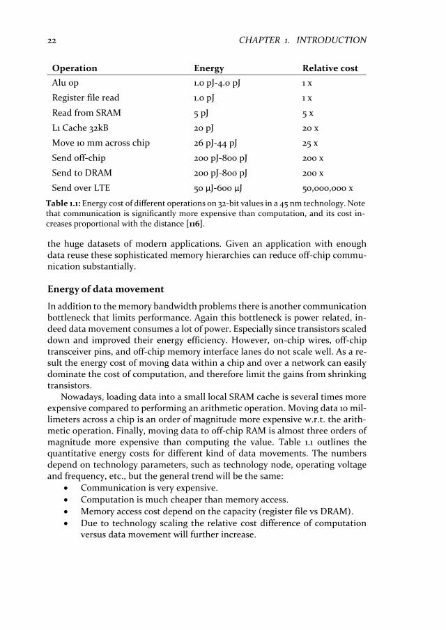
Nowadays, loading data into a small local SRAM cache is several times more expensive compared to performing an arithmetic operation. Moving data 10 mil-limeters across a chip is an order of magnitude more expensive w.r.t. the arith-metic operation. Finally, moving data to off-chip RAM is almost three orders of magnitude more expensive than computing the value. Table 1.1 outlines the quantitative energy costs for different kind of data movements. The numbers depend on technology parameters, such as technology node, operating voltage and frequency, etc., but the general trend will be the same:
• Communication is very expensive.
• Computation is much cheaper than memory access.
• Memory access cost depend on the capacity (register file vs DRAM).
• Due to technology scaling the relative cost difference of computation versus data movement will further increase.
Table 1.1: Energy cost of different operations on 32-bit values in a 45 nm technology. Note that communication is significantly more expensive than computation, and its cost in-creases proportional with the distance [116].
Operation Energy Relative cost
Alu op 1.0 pJ-4.0 pJ 1 x
Register file read 1.0 pJ 1 x
Read from SRAM 5 pJ 5 x
L1 Cache 32kB 20 pJ 20 x
Move 10 mm across chip 26 pJ-44 pJ 25 x
Send off-chip 200 pJ-800 pJ 200 x
Send to DRAM 200 pJ-800 pJ 200 x
Send over LTE 50 μJ-600 μJ 50,000,000 x

1.3. TRENDS IN DEEP NEURAL NETWORK DEVELOPMENT 23
1.3.4 Platform programmability
In the previous sections we studied the trends in transistor scaling and discussed the growing problem of data movement. Both trends show that future platforms are very much power limited, and it seems that faster systems are only possible if their energy efficiency can be improved. This also holds for the ultra-low power scenario where energy efficiency is key.
It is well know that these sources of inefficiency are often caused by the flex-ibility of general-purpose processors. Hameed et al. [58] demonstrate that a ded-icated accelerator can be 500 times more energy-efficient than a general purpose multiprocessor. The main differences are in the customized local memory data structures and the programming model. Both significantly reduce the applica-tion flexibility, and they improve energy efficiency. This extreme example of en-ergy-efficiency improvement motivates a shift to more heterogeneous compute platforms. In the domain of Smartphones we clearly see this trend, e.g. platforms like Samsung’s Exynos filled multiple dedicated accelerator cores (see Figure 1.17) are no exception. This results in heterogeneous systems with large cores to provide compute power when necessary, and small efficient cores for normal mode.
Although specialized cores can improve energy-efficiency they pose a major challenge for programmers. Currently, there are already significant programma-bility issues with normal multicore processors and GPUs. On a set of throughput computing benchmarks it is shown that natively written C/C++ code that is par-allelism unaware is on average 24x (up to 53x) slower than the best-optimized code on a recent 6-core Intel Core i7 [129]. Note that this is for a general purpose processor that is designed to be flexible. In a heterogeneous context this slow-down is much bigger. Getting the best multicore performance requires the use of concepts such as parallel threads and vector instructions. In addition, making
Figure 1.17: Die photo of Samsung’s Exynos Octa SoC. It contains a big and a small ARM quad core CPU, a GPU, and multiple accelerators for video, audio, and image processing.
24 CHAPTER 1. INTRODUCTION
effective use of the memory hierarchy requires is very challenging code transfor-mations.
Due to the dark silicon energy problems future heterogeneous platforms will have multiple cores and accelerators, each with their ISA (Instruction Set Archi-tecture, x86 or ARM), different type of parallelism (threads, vectors), a shared or their own memory space, a custom memory hierarchy. This will result in an even more challenging programming environment where much more programming effort will be required to optimize applications. We conclude that the increased complexity of heterogeneous platforms in the near future will increase the per-formance gap between native and optimized code.
1.4 Problem statement
In the previous sections the trends in deep neural network development were discussed. It seems that the size (in number of model parameters) is key for their recent success in many application domains. Continuing the existing exponen-tial trend of larger and deeper networks will likely result in even more advanced applications, and record breaking accuracy on complicated classification prob-lems. Pushing the deep neural network processing forward is one interesting di-rection. However, the usage of existing and future deep learning technologies in our daily life could be a game changer. It would give our personal companion devices the intelligence to help us with many complicated decisions.
The problematic part that prevents us from running deep neural nets on the class of embedded or always on portable devices is their huge computational workload. The embedded platforms of today simply do not have the processing capabilities to run such applications in real-time. For example, running a rela-tively shallow ConvNet for Speed Sign detection on a popular embedded plat-form (containing an ARM cortex-A9) results in a frame rate of 0.43 fps, which is far below acceptable. After studying the trends in microprocessor development we can conclude that it is not likely that the large performance gap will be closed any soon by new and more powerful embedded platforms.
As of today almost all compute platforms are power constrained, from the large super computers to the wearable system domain. The computational trends that are outlined in the previous section reveal that there are multiple problems that will slow down progress in compute performance for the coming years. Important issues are:
• The failure of Dennard scaling since 2005, disabled a large part of the en-ergy-efficiency advantage of new and smaller transistor technology gener-ations [42];
• The memory bottleneck and the increasing portion of energy that’s con-sumed by data movement in current compute platforms;
• The huge programmability issues that become even worse since computer architects try to cope with the energy problem by moving towards more specialized heterogeneous architectures.

1.5. CONTRIBUTIONS 25
For the application domain of deep neural networks the current compute prob-lems can stop or at least slow down further embedded use of deep learning. Even more problematic is the fact that these compute problems reduce the applica-bility of this state-of-the-art technology. To make that step from benchmarks towards real products and life changing solutions substantial improvements are required.
The goal of this thesis is to substantially improve the efficiency of deep con-volutional networks. This improvement should enable the final technological step that moves the applicability of deep convolutional networks from offline only (cloud based) scenarios to the real-time portable and even wearable use-cases.
Efficiency is defined by three quantitative properties: 1. The number of compute operations that are required (Compute); 2. The number of necessary external memory transfers (Data Movement); 3. The amount of utilization that a normal programmer achieves when
mapping different network workloads (Flexibility). In the end all three efficiency properties influence the energy-efficiency.
1.5 Contributions
This thesis focusses on addressing the efficiency problems when running Deep Neural Network applications. In this work the problems are addressed on mul-tiple fronts that span opportunities on the algorithmic side all the way down to the platform side. Our efforts to improve efficiency are published in [103,108,104,102,109,107]. Although the main focus is on Deep Convolutional Net-works it is important to realize that many of the contributions are applicable to other applications, in particular the image processing and vision aplications. The main contributions of this these can be summarized as:
1. An algorithmic modification to the feature extraction layers of Convo-lutional Networks. The modification merges the convolution and sub-sampling layers of these networks [103]. This layer merging reduces the computational and data transfer workloads of Convolutional Networks.
2. A new method for data locality optimization named inter-tile reuse op-timization [104]. This method is developed to exploit the knowledge that for many accelerators workloads with a static schedule the future data content is known. This is directly applicable to Convolutional networks and increases the amount of utilized data reuse by a significant amount upon the state-of-the-art.
3. The Neuro Vector Engine (NVE) a flexible and programmable accelera-tor architecture for Convolutional Networks [109]. This is an ultra-low power accelerator that is designed for flexibility such that many differ-ent Convolutional Network workloads run close to full utilization.
4. An optimizing compiler framework for the NVE accelerator template. From abstract and simple network specification the compiler generates

26 CHAPTER 1. INTRODUCTION
close to optimal code (fully utilizing the NVE data path). Important to note is that the NVE is the first Deep Learning accelerator with an opti-mizing VLIW compiler [107]. This directly increases the applicability and ease of use in future SoC’s.
This work shows that optimizations in multiple domains can drastically im-prove the energy-efficiency of deep convolutional networks. This is demon-strated by using the first two contributions for mapping on the NVE design. Combined the presented contributions address the challenges posed in our problem statement. As a result these contributions enables future mobile and wearable platforms to run Convolutional Network applications.
1.6 Thesis outline
After this motivational introduction chapter this thesis will continue with ex-plaining background of deep convolutional networks in Chapter 2. This chapter provides the necessary background information to understand the later contri-butions.
In Chapter 3 our two baseline applications are defined. These are two differ-ent convolutional networks that will be used throughout the thesis: 1) Speed Sign Detection and Classification [105]; 2) A face detection network based upon [53]. Both applications are trained and their conversion to a video processing appli-cation is discussed. For both applications we will give the naïve C based mapping results.
Our main contributions are presented in the Chapters 4 to 7. In Chapter 4 we start with the merging of feature extraction layers [103]. We show theoretical gains of this optimization and we evaluate and verify these gains with a CPU and a GPU mapping. Chapter 5 describes our inter-tile reuse optimization method-ology [104]. We evaluate the effectiveness of inter-tile reuse optimization on var-ious accelerator workloads, to show the broad applicability of our technique. Our evaluation metrics are external memory transvers, FPGA resource costs and FPGA execution time, all based upon accelerator architecture templates that can be used with high-level synthesis tools [108]. Chapter 6 introduces the template for the Neuro Vector Engine (NVE) [109]. Our optimizing VLIW compiler [107] is presented and evaluated in Chapter 7.
Finally, in Chapter 8 we conclude the thesis and summarize possible direc-tions for future work. This thesis does not contain a separate related work chap-ter. The relevant related work is discussed per chapter.
27
2.
DEEP CONVOLUTIONAL NETWORKS
During the last decade Deep Convolutional Networks (ConvNets) have rig-orously changed the domains of computer vision and pattern recognition. Many of these results are achieved because these nets are able to combine domain knowledge of the problem and machine learning from huge amounts of data. In this background chapter the different concepts and their motivations for the structure of ConvNets are discussed. This shows the differences and similarities with classical neural networks. ConvNets benefit from simple operators that are applied many times on input to build feature hierarchies. Different layer types such as convolution or pooling layers are discussed with their motivations. By stacking these layer module deep classification machines are constructed that can give impressive clas-sification result.
2.1 Introduction
As illustrated in the previous chapter, neural networks where used successfully for simple pattern recognition problems. Later, researchers realized that these algorithms and networks where too simplistic to solve more complicated and real-world pattern recognition problems. Section 1.1 concludes with the general-ization issues of so called ‘shallow’ neural network models. Adding more free parameters to a two layers neural network does not solve this issue, but it makes the generalization problem even worse.
In Section 1.2 we briefly touched the topic of deep networks that stack many layers to improve the classification accuracy and prevent overfitting. We have shown that it is not only the depth of these nets but especially the structural constraints that make that these deeper nets are so successful. Building prior information in neural networks is key to achieve a good generalization. Tech-niques such as receptive fields and weight sharing are the basis for modern deep
CHAPTER

28 CHAPTER 2. CONVOLUTIONAL NETWORKS
Convolutional Networks (ConvNets). It enabled the construction of complicated feature extraction hierarchies that gave a tremendous boost to machine vision.
This background chapter should give the reader a clear understanding of the structure in ConvNets. Outlining how neural networks evolved into these deep classification machines? That information is required to understand the later optimization Chapters 4, 5, 6, and 7. In these later chapters we propose methods to reduce the increasing network complexity. This to ensure that these powerful classifier models can be implemented on resources constrained mobile devices. Which should give intelligent features to or next generation of companion de-vices. The task of training deep convolutional networks is covered in Chapter 3, where we develop our benchmark applications. The details of gradient propaga-tion for learning is covered in more detail in Chapter 4, where this matter is needed to evaluate our layer merging operations.
In this chapter an introduction into visual data processing is given in Section 2.2. In Section 2.3 we cover the motivations that resulted into convolution oper-ations to process visual data. From the need for parameter reduction by convo-lutions we go over the different types of layers in a ConvNet. The methods to construct powerful classifiers out of the different layer modules are discussed in Section 2.4. In Section 2.5, recent advances are discussed that enabled the use of even deeper networks resulting in a depth of 152 layers. Section 2.6 end this chap-ter with a summary and conclusions from this ConvNet background chapter.
2.2 Challenges of visual data processing
In Chapter 1.2 we briefly discussed the intriguing challenges of visual object recognition. Humans solve it without much effort, but for computer algorithms it is a very challenging task. In this section we discuss the properties of visual data and analyze how visual data is different from feature vectors. With feature vectors we refer to a set of features like the ones used to classify a person’s health, e.g., “age”, “nationality”, “weight”, “length”, “blood pressure”, “respiratory rate”, “heart rate”, “oxygen saturation”, and “gender”.
One of the first observations that sets visual data apart from feature vectors is the huge dimensionality. As illustrated by Figure 2.1, a road scene image for speed sign recognition easily contains 2.76 Million input variables. This involves three channels RGB of a 72op HD video frame. If this problem is reduced to sin-gle sign detection the frame size could be reduced to a 32 x 32 pixel grayscale patch; see Figure 2.2. Still the patch contains 1,024 input variables. A simple two-layer neural network with 1,024 hidden neurons and one output neuron has 1 Million parameters. This is a huge number of network parameters, especially compared with networks that classify on feature vectors. For example the health classification network has an input vector of 9 values. With 9 hidden neurons and one output neuron the network has 100 parameters. This is a difference of four orders of magnitude compared with a simple speed sign detector. It clearly illustrates the huge dimensionality challenges involved in visual images.

2.2. CHALLENGES OF VISUAL DATA PROCESSING 29
On the other hand visual data mainly contains inputs that are locally corre-lated. If we shift an image by a few pixels the image contents is still very similar. However, the input vector changed a lot. This effect is demonstrated in Figure 2.2 where changes like shift, scaling, or rotation do not change the local correla-tion between variables. In all cases a speed sign has large regions of white pixels. This is very different for feature based vector representations. Table 2.1 demon-strates that an element shift in the health classification vector would result in a vector that does not make any sense, i.e. there is no local correlation between elements.
Age Nation-
ality Weight Length
Blood pressure
Resp. rate
Heart rate
Gender
33 Dutch 80 1.88 120 13 60 Male Male 33 Dutch 80 1.88 120 13 60
Table 2.1: A small shift in the feature vector of the health classification problem would result in a very strange input vector. However, for images a one element offset is very common.
We conclude that image data is very high dimensional, which poses chal-lenges such as overfitting on the data. Furthermore, we conclude that the indi-vidual elements of image data can be very different after a subtle change in the image. For example a shift or illumination change will often modify all individual elements. Therefore image data requires a different approach. It requires a focus on the local correlations. Absolute pixel values alone do not describe the infor-mation in an image, it are the local patterns that best describe the image content.
Input dimensionality: 720 x 1,280 x 3 = 2,764,800
Figure 2.1: A720 x 1,280 RGB road scene image for speed sign recognition has a huge input dimensionality of 2.76 Million input variables.
shift x, y scale rotate
local correlation of variables
gray 32x32 = 1,024 val.
Figure 2.2: Visual data has a huge dimensionality even a grayscale 32x32 pixel speed sign image consists of 1,024 variables. Small visual changes like a shift, scale, or rotate have a big impact on all variables. However, there is local structure between variables that re-mains similar after a visual change. For example the regions of neighbouring white pixels do exist in all versions of the speed sign images.
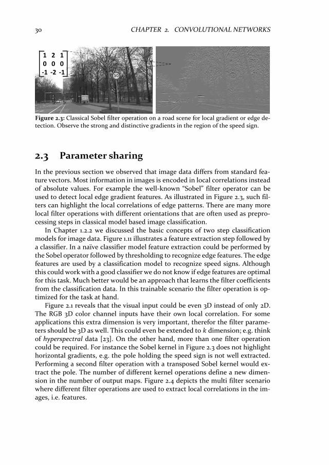
30 CHAPTER 2. CONVOLUTIONAL NETWORKS
2.3 Parameter sharing
In the previous section we observed that image data differs from standard fea-ture vectors. Most information in images is encoded in local correlations instead of absolute values. For example the well-known “Sobel” filter operator can be used to detect local edge gradient features. As illustrated in Figure 2.3, such fil-ters can highlight the local correlations of edge patterns. There are many more local filter operations with different orientations that are often used as prepro-cessing steps in classical model based image classification.
In Chapter 1.2.2 we discussed the basic concepts of two step classification models for image data. Figure 1.11 illustrates a feature extraction step followed by a classifier. In a naïve classifier model feature extraction could be performed by the Sobel operator followed by thresholding to recognize edge features. The edge features are used by a classification model to recognize speed signs. Although this could work with a good classifier we do not know if edge features are optimal for this task. Much better would be an approach that learns the filter coefficients from the classification data. In this trainable scenario the filter operation is op-timized for the task at hand.
Figure 2.1 reveals that the visual input could be even 3D instead of only 2D. The RGB 3D color channel inputs have their own local correlation. For some applications this extra dimension is very important, therefor the filter parame-ters should be 3D as well. This could even be extended to 𝑘 dimension; e.g. think of hyperspectral data [23]. On the other hand, more than one filter operation could be required. For instance the Sobel kernel in Figure 2.3 does not highlight horizontal gradients, e.g. the pole holding the speed sign is not well extracted. Performing a second filter operation with a transposed Sobel kernel would ex-tract the pole. The number of different kernel operations define a new dimen-sion in the number of output maps. Figure 2.4 depicts the multi filter scenario where different filter operations are used to extract local correlations in the im-ages, i.e. features.
1 2 10 0 0-1 -2 -1
Figure 2.3: Classical Sobel filter operation on a road scene for local gradient or edge de-tection. Observe the strong and distinctive gradients in the region of the speed sign.

2.3. PARAMETER SHARING 31
Detecting local correlations can be parameter efficient. For example, the 6 extraction filters in Figure 2.4 require only 450 parameters. If we apply this op-eration on 3 color channels of 32 x 32 pixel speed signs it would result in 6 output maps of 28 x 28 values. The reduced number of output resolution is caused since the filter is applied only to the valid part of the image.
A fully connected neural network with the same number of outputs would require a massive amount of parameters. In this case 28 x 28 x 6 hidden neurons, each having 32 x 32 x 3 inputs (fully connected), resulting into 14.5 million pa-rameters. In chapter 1.2.1 the concept of receptive fields for neurons was ex-plained. Using a 5 x 5 x 3 receptive fields for each hidden layer neuron the parameter set is reduced to 353 thousand parameters. Both neural net imple-mentations use way too many parameters for the speed sign classification prob-lem. It would give two major problems:
1. The model would suffer from overfitting on the problem. Using many training examples and regularization techniques [69] could help reduc-ing the overfitting.
2. The computational workload involved when evaluating such a model is huge.
For image data it seems that weight sharing by using convolutions is much more efficient compared to fully connected layers; even receptive fields use too many parameters to be efficient.
5
5
3
RGB 3 Channels
Convolution
1 result channel per filter
6 output channels
=
Figure 2.4: Multiple filter operations applied to an RGB input patch. Filter operations are performed by convolution with a set of filter coefficients. These coefficients are tuned to extract the important local correlations in the image data, e.g. gradient detection for dif-ferent orientations.
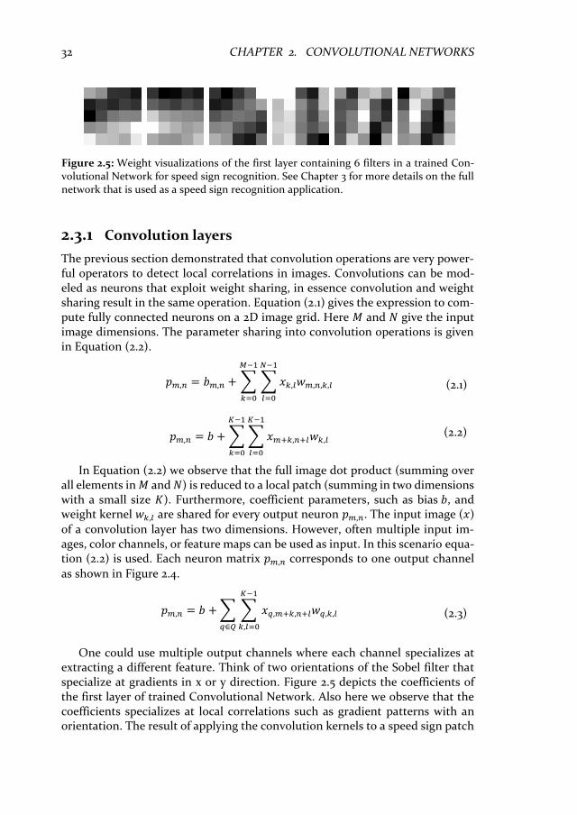
32 CHAPTER 2. CONVOLUTIONAL NETWORKS
2.3.1 Convolution layers
The previous section demonstrated that convolution operations are very power-ful operators to detect local correlations in images. Convolutions can be mod-eled as neurons that exploit weight sharing, in essence convolution and weight sharing result in the same operation. Equation (2.1) gives the expression to com-pute fully connected neurons on a 2D image grid. Here 𝑀 and 𝑁 give the input image dimensions. The parameter sharing into convolution operations is given in Equation (2.2).
𝑝𝑚,𝑛 = 𝑏𝑚,𝑛 + ∑ ∑𝑥𝑘,𝑙𝑤𝑚,𝑛,𝑘,𝑙
𝑁−1
𝑙=0
𝑀−1
𝑘=0
(2.1)
𝑝𝑚,𝑛 = 𝑏 +∑∑𝑥𝑚+𝑘,𝑛+𝑙𝑤𝑘,𝑙
𝐾−1
𝑙=0
𝐾−1
𝑘=0
(2.2)
In Equation (2.2) we observe that the full image dot product (summing over all elements in 𝑀 and 𝑁) is reduced to a local patch (summing in two dimensions with a small size 𝐾). Furthermore, coefficient parameters, such as bias 𝑏, and weight kernel 𝑤𝑘,𝑙 are shared for every output neuron 𝑝𝑚,𝑛. The input image (𝑥)
of a convolution layer has two dimensions. However, often multiple input im-ages, color channels, or feature maps can be used as input. In this scenario equa-tion (2.2) is used. Each neuron matrix 𝑝𝑚,𝑛 corresponds to one output channel
as shown in Figure 2.4.
𝑝𝑚,𝑛 = 𝑏 +∑ ∑ 𝑥𝑞,𝑚+𝑘,𝑛+𝑙𝑤𝑞,𝑘,𝑙
𝐾−1
𝑘,𝑙=0𝑞∈𝑄
(2.3)
One could use multiple output channels where each channel specializes at extracting a different feature. Think of two orientations of the Sobel filter that specialize at gradients in x or y direction. Figure 2.5 depicts the coefficients of the first layer of trained Convolutional Network. Also here we observe that the coefficients specializes at local correlations such as gradient patterns with an orientation. The result of applying the convolution kernels to a speed sign patch
Figure 2.5: Weight visualizations of the first layer containing 6 filters in a trained Con-volutional Network for speed sign recognition. See Chapter 3 for more details on the full network that is used as a speed sign recognition application.

2.3. PARAMETER SHARING 33
is given in Figure 2.6b. The descriptive local gradients are highlighted in the 6 feature maps.
2.3.2 Pooling layers
Convolution layers often use multiple kernels to extract different features. The example illustrated by Figure 2.4 generates 6 feature maps of 28x28 neurons re-sulting in 4704 values. The three channel 32x32 pixel input consisted of 3072 values, so the convolution layer significantly increased the amount of data. For efficient classification only descriptive features are required, so probably not all features are required.
Pooling layers are used to aggregate multiple feature values into a single value, see Figure 2.6a. This reduces the resolution in feature maps, but it should preserve important features. Figure 2.6b illustrates the data reduction achieved by a pooling layer. Another desirable effect of feature pooling is invariance to small transformations. A feature grid that shifts a position will still propagate into the pooling result.
In general there are two popular pooling strategies: 1) Average pooling is very similar to the operation in a convolution layer. The main difference is that a single weight is used instead of a kernel. Furthermore, a stride is used to achieve the data reduction. Equation (2.4) gives the operation for average pooling. A scale coefficient 𝑤 and a bias 𝑏 are the trainable values in this layer.
input
convolution layer pooling
layer
a00 a01
a10 a11
c20 c21
c30 c31
d22 d23
d32 d33
b02 b03
b12 b13
a b
c d
pooling reduction
a) b)
Figure 2.6: a) Pooling operation aggregates multiple values into a single value. b) First layers of the speed sign recognition net illustrating data reduction and feature selection by pooling.

34 CHAPTER 2. CONVOLUTIONAL NETWORKS
𝑝𝑚,𝑛 = 𝑏 + 𝑤 ∑ 𝑥𝑚𝑆+𝑘,𝑛𝑆+𝑙
𝑆−1
𝑘,𝑙=0
(2.4)
2) Max pooling selects the local maximum from a window by using the max () operator as given in equation (2.5). Max pooling does not involve any trainable parameter. It differs from average pooling that has a weight and bias.
𝑝𝑚,𝑛 = max0≤𝑘<𝑆,0≤𝑙<𝑆
(𝑥𝑚𝑆+𝑘,𝑛𝑆+𝑙) (2.5)
Both pooling functions use a scale factor 𝑆 as a reduction parameter. This parameter defines the distance between neighboring windows. In the presented examples the pooling windows do not overlap, but pooling with overlap is also a valid option.
2.3.3 Neuron layers
For completeness we give the definition of classical neuron layers. There is no parameter sharing in neuron layers, every neuron has his own set of weights. The neuron layer operation on an image was given in Equation (2.1). Similar as for convolution layers the neuron layer operation can be extended to multiple input feature maps. Note that not all neuron layers are fully connected to all input feature maps. To keep all notations the same one could define a neuron layer with convolution operations. These convolutions have only a single output point so it is not a shifting window over the image, but a single position. In case the input of a neuron layer is a neuron layer we could use a 1x1 kernel for convolu-tion. Further details regarding neuron layers is given in chapter 1.
2.3.4 Normalization layers
Some networks use fixed normalization structures in a few layers. These normal-izations enforce group behavior like sparsity or they normalize the mean and variance in a feature map. Local response normalization is one of these normali-zation structures. It implements competition between neurons at the same lo-cation, but in different feature maps. Popular competition winning networks like the ImageNet winner from 2012 use local response normalization to improve the generalization [79]. Local response normalization is performed by the operation in equation (2.6). The input activities 𝑥𝑞,𝑚𝑛 for neighboring feature map posi-
tions 𝑞 are used to normalize each neuron output 𝑝𝑟,𝑚,𝑛. The constants 𝑘, 𝑛, 𝛼,
and 𝛽 are hyper-parameters that must be tuned carefully.
𝑝𝑟,𝑚,𝑛 = 𝑥𝑟,𝑚,𝑛 (𝑘 + 𝛼 ∑ (𝑥𝑞,𝑚,𝑛)2
min(𝑁−1,𝑟+𝑛/2)
𝑞=max(0,𝑟−𝑛 2⁄ )
)
𝛽
⁄ (2.6)

2.4. CONSTRUCTING A CONVOLUTIONAL NETWORK 35
Recently, Batch Normalization [73] is introduced which replaced local response normalization. Batch normalization improves the training process of a network by adding normalization layers that normalize small sets of training examples (mini-batches).
We mention these two normalization layer types for completeness. Although some of our proposed optimization methods are applicable to both techniques we do not further evaluate them in this thesis.
2.4 Constructing a convolutional network
In the previous section we demonstrated that local correlations in image data can be extracted by convolution layers. In addition to feature extraction a pool-ing operation can be used to select only important features. However, these two operations alone do not make a classifier. For this we should stack layer opera-tions together and compute towards a classification label. Each of the presented layer types can be used as compute modules that perform a transformation on the intermediate data.
For instance, classification of a grayscale speed sign patch could use multiple convolutional layers. Each convolutional layer can use a non-linear activation function. In chapter 1 we discussed several activation functions. After each acti-vation function a pooling step with or without another activation can be used to reduce the data. After a few cascades of this convolution, activation, and pooling structure the image is converted into a feature vector. Depending on the size of the input patch and the different kernel parameters this can be few cascades or many, like 5 or even more. Figure 2.7 depicts a ConvNet that reduces the 32x32 grayscale patch to a 16x5x5 value feature vector. In this case a relatively small patch is converted. When the classified objects are larger often much deeper networks are used. For example, the VGG [138] ImageNet 2014 submission uses 16 convolution and 5 pooling layers to convert 224x224 patches into a feature vector of 512x7x7. The convolution layers use small 3x3 kernels that can still de-scribe left/right, up/down, or center gradients. The inputs of convolution layers
inputconvolution
layer 1activation function 1
pooling layer 1
convolution layer 2
activation function 2
pooling layer 2
neuron layer 5
neuron layer 6
Feature Extraction Classification
1 map 32x32 6 maps 28x28 6 maps 28x286 maps 14x14 16 maps 10x10 16 maps 10x10 16 maps 5x5
80 neurons 1x1
8 neurons 1x1
Figure 2.7: Convolutional network architecture for speed sign recognition. Stacking sev-eral convolution, activation, and pooling combinations to obtain a feature vector. Con-tinue processing with a few neuron layers to converge to a classification label.
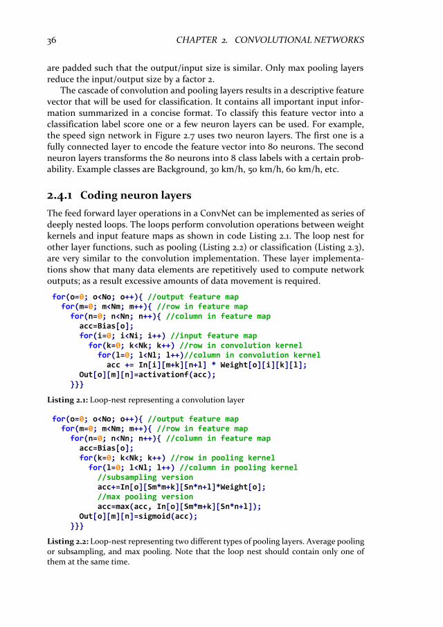
36 CHAPTER 2. CONVOLUTIONAL NETWORKS
are padded such that the output/input size is similar. Only max pooling layers reduce the input/output size by a factor 2.
The cascade of convolution and pooling layers results in a descriptive feature vector that will be used for classification. It contains all important input infor-mation summarized in a concise format. To classify this feature vector into a classification label score one or a few neuron layers can be used. For example, the speed sign network in Figure 2.7 uses two neuron layers. The first one is a fully connected layer to encode the feature vector into 80 neurons. The second neuron layers transforms the 80 neurons into 8 class labels with a certain prob-ability. Example classes are Background, 30 km/h, 50 km/h, 60 km/h, etc.
2.4.1 Coding neuron layers
The feed forward layer operations in a ConvNet can be implemented as series of deeply nested loops. The loops perform convolution operations between weight kernels and input feature maps as shown in code Listing 2.1. The loop nest for other layer functions, such as pooling (Listing 2.2) or classification (Listing 2.3), are very similar to the convolution implementation. These layer implementa-tions show that many data elements are repetitively used to compute network outputs; as a result excessive amounts of data movement is required.
for(o=0; o<No; o++){ //output feature map for(m=0; m<Nm; m++){ //row in feature map for(n=0; n<Nn; n++){ //column in feature map acc=Bias[o]; for(i=0; i<Ni; i++) //input feature map for(k=0; k<Nk; k++) //row in convolution kernel for(l=0; l<Nl; l++)//column in convolution kernel acc += In[i][m+k][n+l] * Weight[o][i][k][l]; Out[o][m][n]=activationf(acc); }}}
Listing 2.1: Loop-nest representing a convolution layer
for(o=0; o<No; o++){ //output feature map for(m=0; m<Nm; m++){ //row in feature map for(n=0; n<Nn; n++){ //column in feature map acc=Bias[o]; for(k=0; k<Nk; k++) //row in pooling kernel for(l=0; l<Nl; l++) //column in pooling kernel //subsampling version acc+=In[o][Sm*m+k][Sn*n+l]*Weight[o]; //max pooling version acc=max(acc, In[o][Sm*m+k][Sn*n+l]); Out[o][m][n]=sigmoid(acc); }}}
Listing 2.2: Loop-nest representing two different types of pooling layers. Average pooling or subsampling, and max pooling. Note that the loop nest should contain only one of them at the same time.

2.5. DEEPER NETWORKS 37
for(o=0; o<No; o++){ //output feature map for(m=0; m<Nm; m++){ //row in feature map for(n=0; n<Nn; n++){ //column in feature map acc=Bias[o]; for(i=0; i<Ni; i++) //input feature map acc+=in[i][m][n]*weight[o][i]; out[o][m][n]=sigmoid(acc); }}}
Listing 2.3: Loop-nest representing a neuron based classification layer.
2.5 Deeper networks
The early multilayer perceptron’s often used two layers, one hidden layer and one output layer. These ‘shallow’ classifiers did not generalize well when trained on raw pixel values. Often these classifiers required good feature extractors that reduce the high dimensional pixel space into feature representations. The intro-duction of Convolutional Networks [84] provided a framework where feature extraction could be combined with classification in a single end-to-end trainable model. By enforcing structural constraints into the first layers of a network these ConvNets where able to use 5 to 8 layers of non-linear transformations effi-ciently. Each layer extracts a set of features starting with simple gradients to-wards more complicated shapes that are built on top of preceding layer features. Due to a larger number of layers these nets can implement complicated func-tions of its inputs.
Training a network with a depth beyond 8 layers is rather challenging. This is mainly caused by the gradient based training algorithms. Error gradients are used to update coefficients to a new state that performs better on the cost func-tion. In chapter 3 we provide more information on error gradient based optimi-
zation procedures. For now error gradients are defined as 𝜕𝐸
𝜕𝑊, where 𝐸 is a loss
function on the produced labels by the network in function of 𝑊 holding the network weights. The gradients are efficiently computed by the chain rule that requires propagation from network output back to the inputs. Propagating the error gradients from the output cost function back towards the input layers is the difficult part. Sigmoid or hyperbolic tangent activation functions have the problem that they decrease error gradients. The introduction of Rectified Linear Units (ReLUs) improved the training of deep networks a lot [56]. Examples are the networks from 2012 to 2014 that won the ImageNet competition [79,138]. These nets benefit from efficient gradient propagation. The ReLU activation is described by max(0, 𝑥), where 𝑥 is the input signal. Since ReLUs do not decrease gradients it enables training of much deeper networks. In addition, the ReLU activation gives sparsity to the neuron feature encodings in the network due to the zero part. For example, VGG [138] uses ReLU activations and demonstrates up to 21 layers with a total of 280 Million parameters. Such very deep nets stack many feature representations resulting in very advanced classifiers.

38 CHAPTER 2. CONVOLUTIONAL NETWORKS
Recently, researchers successfully trained substantially deeper networks. To propagate the subtle details of a classification problem through more than 20 layers a different approach was required. Instead of learning transformations from 𝑥 to 𝑓(𝑥) they learn only the deltas on 𝑥 and reuse the original 𝑥 to perform the transformation. This is achieved by using Residual blocks that learn the func-tion ℎ(𝑥) = 𝑓(𝑥) + 𝑥. Figure 2.8 shows the structure of residual blocks. Learning only the differences from the input signals of layers enables a huge network depth of 152 layers [63].
This extreme depth has further improved the network complexity. Maybe not directly in the number of free parameters. Some of the deeper nets have fewer trainable parameters. However data movement and data dependencies between results make the computational requirements more challenging. In addition, the parallelism in these deeper networks has become more complicated. Data de-pendencies over layers make that it is more difficult to exploit all parallelism.
2.6 Conclusions
This chapter has discussed the current developments in the field of deep learn-ing that resulted in more powerful networks. By understanding the structure in your data it became possible to embed this knowledge into the classifier archi-tecture. This resulted into parameter sharing by means of convolution layers. Or in the extreme case learning only the deltas upon the input format to increase network depth. All these techniques enabled the use of larger networks, larger in number of free parameters, and deeper in number of layers. As a result the computational challenges when implementing such a network have become much more difficult.
In Chapter 1 we demonstrated that the complexity growth of ConvNets was historically accelerated by the developments in computing platforms. However, a similar pace in compute performance increase for the coming years is not ex-pected. Power limitations are nowadays slowing down the performance growth for each new technology generation. Therefore the remainder of this thesis will
X convolution layer
ReLUlayer
convolution layer
+
f(X)
X
f(X)+X
Figure 2.8: A schematic overview of a Residual learning building block. Multiple blocks can be cascaded, and each block can have a varying depth for network f(X).

2.6. CONCLUSIONS 39
focus on efficiency improvements. We will research and apply high-level algo-rithm modifications and low-level data movement strategies that exploit data reuse. Furthermore this thesis will show a custom accelerator architecture in-cluding advanced optimizing compilers to simplify the mapping.

40
3.
BENCHMARK APPLICATIONS
In the next chapters several methods will be introduced to improve the ef-fectiveness of Deep Convolutional Networks. We need benchmark applica-tions to quantify these improvements. Compute workload models may help to increase the understanding of trade-offs that are made. In addition, real applications on different platforms are used to verify our models. In this chapter we introduce two real-world vision applications for the purpose of benchmarking. A Speed sign recognition application for autonomous driv-ing purposes, and a face detection application for surveillance. For both ap-plications we explain the data collection and training procedure to obtain an accurate and robust ConvNet. Additionally, the conversion from a patch classification network to a video detection application is outlined. Finally we evaluate the performance of our applications on a CPU and a massively parallel GPU platform. Parts of this chapter are based on work presented in the 8th International Automotive Congress 2011 [103]
3.1 Introduction
This thesis proposes multiple contributions that improve the efficiency of deep convolutional networks, so it also requires evaluation. Each contribution can be evaluated by a performance or efficiency model. For example such a model could evaluate the achieved workload reduction. A good model can increase our un-derstanding of the trade-offs that arise when applying optimizations. On the other hand, these models and optimizations should be verified with real data or in our case real-world applications. This ensures that the performance models are correct and it further increases the understanding of the problem. In some cases a real experiment will show unexpected side effects that are very valuable. This holds especially for the machine learning domain where many side effects can occur, e.g. properties such as overtraining and bad generalization can give
CHAPTER
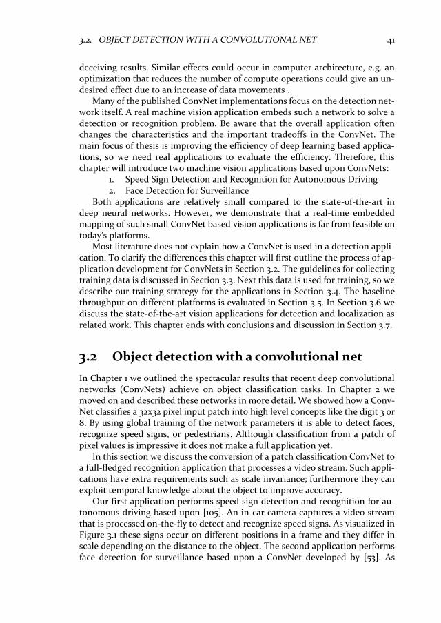
3.2. OBJECT DETECTION WITH A CONVOLUTIONAL NET 41
deceiving results. Similar effects could occur in computer architecture, e.g. an optimization that reduces the number of compute operations could give an un-desired effect due to an increase of data movements .
Many of the published ConvNet implementations focus on the detection net-work itself. A real machine vision application embeds such a network to solve a detection or recognition problem. Be aware that the overall application often changes the characteristics and the important tradeoffs in the ConvNet. The main focus of thesis is improving the efficiency of deep learning based applica-tions, so we need real applications to evaluate the efficiency. Therefore, this chapter will introduce two machine vision applications based upon ConvNets:
1. Speed Sign Detection and Recognition for Autonomous Driving 2. Face Detection for Surveillance
Both applications are relatively small compared to the state-of-the-art in deep neural networks. However, we demonstrate that a real-time embedded mapping of such small ConvNet based vision applications is far from feasible on today’s platforms.
Most literature does not explain how a ConvNet is used in a detection appli-cation. To clarify the differences this chapter will first outline the process of ap-plication development for ConvNets in Section 3.2. The guidelines for collecting training data is discussed in Section 3.3. Next this data is used for training, so we describe our training strategy for the applications in Section 3.4. The baseline throughput on different platforms is evaluated in Section 3.5. In Section 3.6 we discuss the state-of-the-art vision applications for detection and localization as related work. This chapter ends with conclusions and discussion in Section 3.7.
3.2 Object detection with a convolutional net
In Chapter 1 we outlined the spectacular results that recent deep convolutional networks (ConvNets) achieve on object classification tasks. In Chapter 2 we moved on and described these networks in more detail. We showed how a Conv-Net classifies a 32x32 pixel input patch into high level concepts like the digit 3 or 8. By using global training of the network parameters it is able to detect faces, recognize speed signs, or pedestrians. Although classification from a patch of pixel values is impressive it does not make a full application yet.
In this section we discuss the conversion of a patch classification ConvNet to a full-fledged recognition application that processes a video stream. Such appli-cations have extra requirements such as scale invariance; furthermore they can exploit temporal knowledge about the object to improve accuracy.
Our first application performs speed sign detection and recognition for au-tonomous driving based upon [105]. An in-car camera captures a video stream that is processed on-the-fly to detect and recognize speed signs. As visualized in Figure 3.1 these signs occur on different positions in a frame and they differ in scale depending on the distance to the object. The second application performs face detection for surveillance based upon a ConvNet developed by [53]. As
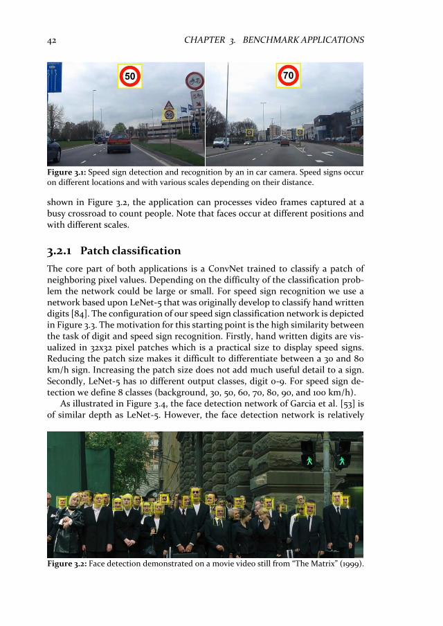
42 CHAPTER 3. BENCHMARK APPLICATIONS
shown in Figure 3.2, the application can processes video frames captured at a busy crossroad to count people. Note that faces occur at different positions and with different scales.
3.2.1 Patch classification
The core part of both applications is a ConvNet trained to classify a patch of neighboring pixel values. Depending on the difficulty of the classification prob-lem the network could be large or small. For speed sign recognition we use a network based upon LeNet-5 that was originally develop to classify hand written digits [84]. The configuration of our speed sign classification network is depicted in Figure 3.3. The motivation for this starting point is the high similarity between the task of digit and speed sign recognition. Firstly, hand written digits are vis-ualized in 32x32 pixel patches which is a practical size to display speed signs. Reducing the patch size makes it difficult to differentiate between a 30 and 80 km/h sign. Increasing the patch size does not add much useful detail to a sign. Secondly, LeNet-5 has 10 different output classes, digit 0-9. For speed sign de-tection we define 8 classes (background, 30, 50, 60, 70, 80, 90, and 100 km/h).
As illustrated in Figure 3.4, the face detection network of Garcia et al. [53] is of similar depth as LeNet-5. However, the face detection network is relatively
Figure 3.1: Speed sign detection and recognition by an in car camera. Speed signs occur on different locations and with various scales depending on their distance.
Figure 3.2: Face detection demonstrated on a movie video still from “The Matrix” (1999).

3.2. OBJECT DETECTION WITH A CONVOLUTIONAL NET 43
sparse; the model has only 947 trainable parameters. Compared to the 50,356 parameters used for speed sign recognition the face detection model is very small. This difference is explained by the complexity of the task. Face detection is a two class problem (background, and face), so the reduced number of model parameters makes sense.
3.2.2 Frame based detection
A patch classifier is not directly useful as video application. Often the classifier is used as sliding window to test for an object at each location and scale in a video frame [147,39]. A naive sliding window search strategy quickly becomes computationally expensive, especially if high resolution frames are used. There-fore advanced search algorithms are developed that search by a smart schedule at the cost of increased control complexity [35]. Many of the complex search patterns introduce data dependencies that reduce the available parallelism.
ConvNets can use an interesting alternative approach to search a full frame. The convolution operator can be performed on any patch size, so the patch is
input36 x 32
feature maps4@32 x 28
5x5convolution
2x2pooling
feature maps4@16 x 14
feature maps14@14 x 12
feature maps14@7 x 6
3x3convolution
2x2pooling
7x6convolution
C1 P1
C2 P2 n1
neurons14
n2
output1
Face
1x1convolution
Figure 3.4: Sparse ConvNet architecture for face detection.
input32 x 32
feature maps6@28 x 28
5x5convolution 2x2
pooling
feature maps6@14 x 14
feature maps16@10 x 10 feature maps
16@5 x 5
5x5convolution
2x2pooling
fullyconnected
or 1x1 convolution
C1P1
C2
P2 n1
n2
sign30 km/h
90 km/h100 km/h
outputs8
5x5convolution
neurons120
Figure 3.3: Dense ConvNet architecture for speed sign recognition.
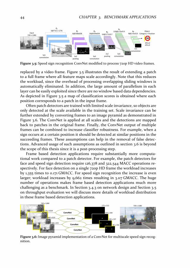
44 CHAPTER 3. BENCHMARK APPLICATIONS
replaced by a video frame. Figure 3.5 illustrates the result of extending a patch to a full frame where all feature maps scale accordingly. Note that this reduces the workload, since the overhead of processing overlapping sliding windows is automatically eliminated. In addition, the large amount of parallelism in each layer can be easily exploited since there are no window based data dependencies. As depicted in Figure 3.5 a map of classification scores is obtained where each position corresponds to a patch in the input frame.
Often patch detectors are trained with limited scale invariance, so objects are only detected at the scale available in the training set. Scale invariance can be further extended by converting frames to an image pyramid as demonstrated in Figure 3.6. The ConvNet is applied at all scales and the detections are mapped back to patches in the original frame. Finally, the ConvNet output of multiple frames can be combined to increase classifier robustness. For example, when a sign occurs at a certain position it should be detected at similar positions in the succeeding frames. These assumptions can help in the removal of false detec-tions. Advanced usage of such assumptions as outlined in section 3.6 is beyond the scope of this thesis since it is a post-processing step.
Frame based detection applications require substantially more computa-tional work compared to a patch detector. For example, the patch detectors for face and speed sign detection require 126,378 and 322,544 MACC operations re-spectively. For face detection on a single 720p HD frame the workload increases by 1,355 times to 0.171 GMACC. For speed sign recognition the increase is even larger; workload increases by 9,662 times resulting in 3.117 GMACC. The huge number of operations makes frame based detection applications much more challenging as a benchmark. In Section 3.4.3 on network design and Section 3.5 on throughput evaluation we will discuss more details of workload distribution in these frame based detection applications.
720 x 1280
720 x 1280
576 x 1024
460 x 819
368 x 655
173 x 313
135 x 249
108 x 197
85 x 156
ConvNet
ConvNet
ConvNet
ConvNet
Figure 3.6: Image pyramid implementation of a ConvNet for multiscale speed sign recog-nition.
input720 x 1280
P1
6@358x638P2
16@177x317
n1
120@173x313 n2
8@173x313Object
Category + Position
5x5 convolution
2x2 pooling
5x5 convolution
1x1 convolution
at(x,y)at(x,y)
C1
6@716 x 1276 C2
16@354x634
2x2 pooling5x5
convolution
Figure 3.5: Speed sign recognition ConvNet modified to process 720p HD video frames.

3.3. DATASET CONSTRUCTION 45
3.3 Dataset construction
A very important element in the development of robust and accurate ConvNet applications is the dataset used for training. Each layer relies on patterns in the data, e.g., to extract the best features that increase class separation for robust classification. As a result, the dataset should be representative for the classifica-tion problem, e.g. for face detection normal faces must be included but also faces with a moustache or sunglasses. This is not specific for ConvNets, other works have shown that large datasets with a good variety of examples result in classifi-ers with excellent generalization and accuracy [99]. In this section dataset col-lection for our benchmark applications is outlined. We mainly show the procedure for our speed sign recognition network; to reduce redundancy we summarize only the differences for face recognition. Note that most of these techniques can be found in other works, so we discuss them for sake of repro-ducibility of our experiments.
Construction of the dataset for speed sign recognition is done by gathering real-world examples. One part is collected by using the Google image search en-gine for speed signs in the Netherlands. The other part consist of images that are obtained with Google Street View. In addition, the training set is increased with a representative data set that was published [98]. Finally the used data set con-tained 713 images of speed signs, which are cropped to show the full sign with a small background border. A subset of the training images is depicted in Figure 3.7. Training with these real-world examples creates invariance for natural vari-ations such as, light conditions, small scale differences, and perspective.
Traffic sign images alone are not sufficient to train a classifier; additionally good set of background images is required. This background training class pre-vents false detections and is therefore very important. Example images from our background class are shown in Figure 3.8. One part of our background class con-tains random image patches that are collected from road scene images. A second part contains traffic sign images that look very similar to the speed sign classes.
30 km/h 50 km/h 60 km/h 70 km/h 80 km/h 90 km/h 100 km/h
Figure 3.7: Example images from the collected traffic sign dataset.
Background images hard to suppress Random background image patches
Figure 3.8: Example images from the speed sign background class.

46 CHAPTER 3. BENCHMARK APPLICATIONS
To test the generalization of the classifier a small part (1/7) of the training set is excluded and later used for testing. An overview of the dataset organization is depicted in Table 3.1. Collecting a speed sign dataset of this size is time consum-ing but necessary to obtain a robust benchmark application. To our knowledge little effort is done to publicize real-world speed sign image databases. Also the fact that speed signs differ from country to country makes it valuable to publicize our dataset1. Additionally our public data set increases the reproducibility of the experiments described in this thesis.
The face detector is trained with the popular and public available Labeled Faces in the Wild (LFW) dataset [71]. The set of 13,458 face images from the web is split into 9,992 training and 3,466 testing images. All images contain align-ment and scale coordinates such that it can be automatically cropped to match the ConvNet patch.
3.4 Training a convolutional net for machine vision
In Chapter 2 we introduced the well know error back-propagation algorithm [125]. This algorithm combined with Stochastic Gradient Descent (SGD), is often used for large-scale learning problems due its high computational efficiency [11]. SGD computes the error gradient for each network parameter and performs small updates in the negative direction of the error to converge to a minimum error. The usage of SGD on a large training set often involves a long script with many problem specific settings to obtain a well-trained network. In this section we outline the procedure that is used for training of our benchmark applications. As in the previous section we mainly discuss the speed sign recognition applica-tion. The differences with face detection are summarized at the end.
1 Our speed sign dataset is publicly available at http://parse.ele.tue.nl/research/speedsign/
Table 3.1: Dataset configuration with the desired output coding for each different class.
Class Output label # Patterns
Training Testing Total
Background 0 0000000 2489 415 2904 30 km/h max 1 1000000 77 13 90 50 km/h max 1 0100000 120 20 140 60 km/h max 1 0010000 62 10 72 70 km/h max 1 0001000 129 21 150 80 km/h max 1 0000100 75 13 88 90 km/h max 1 0000010 79 13 92 100 km/h max 1 0000001 69 12 81
3100 517 3617

3.4. TRAINING A CONVOLUTIONAL NET FOR MACHINE VISION 47
3.4.1 Preprocessing of training data
Before the training procedure is started the data set is prepared. Since both ap-plications use a single input patch the datasets are converted to grey scale im-ages. Although color gives extra information we did not use it because color representations are not very consistent between day and night conditions.
Inspired by the good results for handwritten digit recognition in [137] we ar-tificially increase our data set by applying small modifications to each training sample. Adding such small deformations results in better invariance to the ap-plied distortion, which improves the robustness of the detector. The following distortions are used to expand the training set:
• Light intensity scaling with clipping by a factor [0.8 0.9 1.0 1.1 1.2].
• Shift in x and y position [-2 -1 0 +1 +2] pixel positions.
• Scaling of the images [0.93 1 1.05], the resulting patch is cropped or padded to the original size.
• Face detection patches are flipped over the x axis. The deformations are performed by a function, 𝒙 ← 𝑔(𝒙) that converts patches.
3.4.2 Training loop and recipe
For training a custom MatLab implementation of SGD is used. It is well known that SGD performs very well on large-scale learning problems [5,12]. Problems for which the computing time is the bottleneck are considered large-scale learn-ing. Usually these algorithms are time bound due to the very large number of training iterations. In addition, to being effective SGD is relatively simple which improves the reproducibility our benchmarks.
Although SGD is relatively simple there are many variants and modifications of the algorithm. Additionally, SGD requires multiple hyper-parameters such as, learning rate 𝜂, and epoch size. The training methodology that is used for our benchmarks is outlined in the pseudo description given in Algorithm 3.1. Local gradients diverge over network parameters when computing back from the net-work output to the input. Therefore each layer has a dedicated learning rate 𝜂𝑙 such that layers further from the output use a larger update this equalizes the learning speed over all layers.
The first step in training is parameter initialization. For our benchmarks all coefficients are initialized to small random values taken from the interval
𝜃𝜖 (−1
8,1
8). Advanced training methods sometimes use unsupervised pre-train-
ing to initialize the network parameters [47]. However, the introduction of Rec-tified Linear Units ReLU replaced the need for pre-training in deep networks. We do not discuss pre-training since advanced training methods are beyond the scope of this thesis. After parameter initialization the training loop is entered; every iteration performs one epoch of training succeeded by a test loop to meas-ure generalization. Generalization score 𝐸gen and a predefined number of epochs
is used as stopping criteria. During training a sample is deformed as outlined in
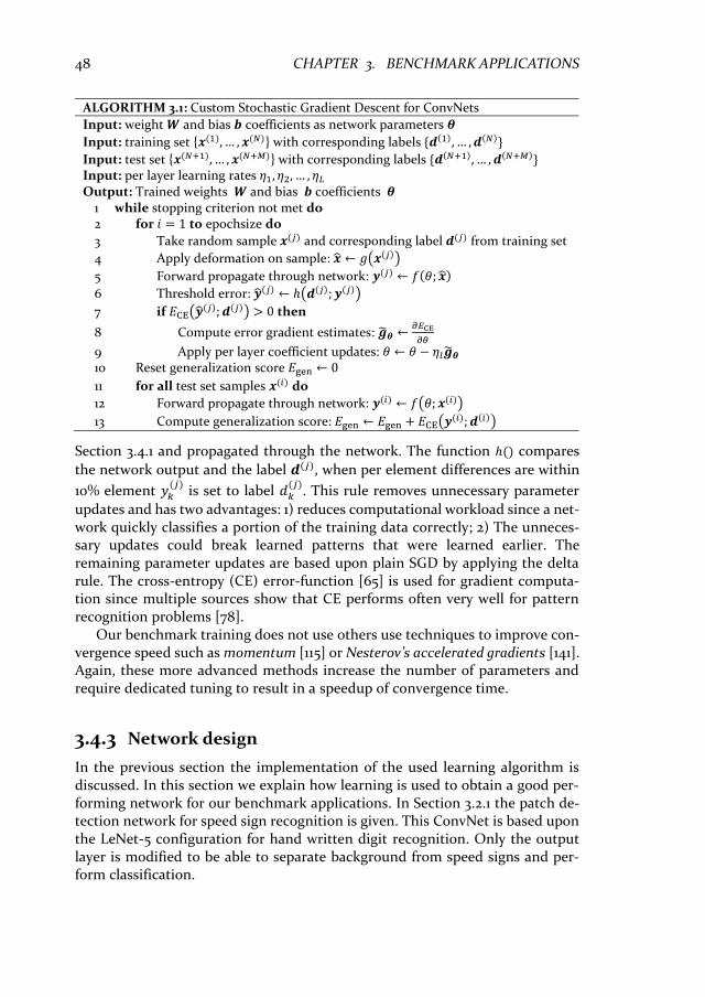
48 CHAPTER 3. BENCHMARK APPLICATIONS
Section 3.4.1 and propagated through the network. The function ℎ() compares
the network output and the label 𝒅(𝑗), when per element differences are within
10% element 𝑦𝑘(𝑗)
is set to label 𝑑𝑘(𝑗)
. This rule removes unnecessary parameter
updates and has two advantages: 1) reduces computational workload since a net-work quickly classifies a portion of the training data correctly; 2) The unneces-sary updates could break learned patterns that were learned earlier. The remaining parameter updates are based upon plain SGD by applying the delta rule. The cross-entropy (CE) error-function [65] is used for gradient computa-tion since multiple sources show that CE performs often very well for pattern recognition problems [78].
Our benchmark training does not use others use techniques to improve con-vergence speed such as momentum [115] or Nesterov’s accelerated gradients [141]. Again, these more advanced methods increase the number of parameters and require dedicated tuning to result in a speedup of convergence time.
3.4.3 Network design
In the previous section the implementation of the used learning algorithm is discussed. In this section we explain how learning is used to obtain a good per-forming network for our benchmark applications. In Section 3.2.1 the patch de-tection network for speed sign recognition is given. This ConvNet is based upon the LeNet-5 configuration for hand written digit recognition. Only the output layer is modified to be able to separate background from speed signs and per-form classification.
ALGORITHM 3.1: Custom Stochastic Gradient Descent for ConvNets
Input: weight 𝑾 and bias 𝒃 coefficients as network parameters 𝜽
Input: training set {𝒙(1), … , 𝒙(𝑁)} with corresponding labels {𝒅(1), … , 𝒅(𝑁)}
Input: test set {𝒙(𝑁+1), … , 𝒙(𝑁+𝑀)} with corresponding labels {𝒅(𝑁+1), … , 𝒅(𝑁+𝑀)} Input: per layer learning rates 𝜂1, 𝜂2, … , 𝜂𝐿 Output: Trained weights 𝑾 and bias 𝒃 coefficients 𝜽
1 while stopping criterion not met do 2 for 𝑖 = 1 to epochsize do
3 Take random sample 𝒙(𝑗) and corresponding label 𝒅(𝑗) from training set
4 Apply deformation on sample: �̂� ← 𝑔(𝒙(𝑗))
5 Forward propagate through network: 𝒚(𝑗) ← 𝑓(𝜃; �̂�)
6 Threshold error: �̂�(𝑗) ← ℎ(𝒅(𝑗); 𝒚(𝑗))
7 if 𝐸CE(�̂�(𝑗); 𝒅(𝑗)) > 0 then
8 Compute error gradient estimates: �̃�𝜽 ←𝜕𝐸CE
𝜕𝜃
9 Apply per layer coefficient updates: 𝜃 ← 𝜃 − 𝜂𝑙�̃�𝜽 10 Reset generalization score 𝐸gen ← 0
11 for all test set samples 𝒙(𝑖) do
12 Forward propagate through network: 𝒚(𝑖) ← 𝑓(𝜃; 𝒙(𝑖))
13 Compute generalization score: 𝐸gen ← 𝐸gen + 𝐸CE(𝒚(𝑖); 𝒅(𝑖))

3.4. TRAINING A CONVOLUTIONAL NET FOR MACHINE VISION 49
In Section 3.2.2 is shown that the video detection application requires 3.117 GMACC operations to evaluate a single 720p video frame, which is a lot. A more detailed analysis reveals that 83% of the workload is required in the first neuron layer n1. Since the overall workload is dominated by layer n1 it makes sense to investigate if it really needs this huge number of parameters. To reduce the computational workload three different configurations of layer n1 are evalu-ated:
1. The original LeNet-5 with 120 neurons in layer n1 is trained as a reference. 2. Layer n1 is reduced to 80 fully connected neurons. 3. n1 contains 40 neurons that are connected to feature map 1 to 8 and an-
other 40 to feature map 9 to 16. Figure 3.9 shows a detailed workload breakdown for the three ConvNet config-urations.
The training progress for the three network configurations is illustrated in Figure 3.10. A magnification of the results during the last 100 epochs shows that network 1 and 3 give the best generalization accuracy. It seems that the 80 neu-rons of network configuration 2 have a somewhat reduced accuracy on the test set. However, by enforcing specific connections in configuration number 3 the generalization performance improves. A reason for the improved performance
0
0.5
1
1.5
2
2.5
3
3.5
C1 S1 C2 S2 N1 N2 total
Wo
rklo
ad [
GM
AC
C]
Layer
n3 120 neuron n3 80 neuron n3 2 sets 40 neurons
Figure 3.9: Workload distribution over layers of the speed sign detection application.
0.00%
5.00%
10.00%
15.00%
20.00%
25.00%
10
110
210
310
410
510
610
710
810
910
1010
1110
1210
1310
1410
1510
1610
1710
1810
1910
Mis
clas
sifi
cati
on
s
Training Epoch
Train net1
Test net1
Train net2
Test net2
Train net3
Test net3
0.00%
0.50%
1.00%
1.50%
2.00%
2.50%
3.00%
1900 1910 1920 1930 1940 1950 1960 1970 1980 1990 2000
Mis
clas
sifi
cati
on
s
Training Epoch
Train net1
Test net1
Train net2
Test net2
Train net3
Test net3
a) b)
Figure 3.10: Per training epoch classification score for speed sign network configuration 1-3. a) Gives the accuracy over 2000 training epochs. b) Highlights the final accuracy.

50 CHAPTER 3. BENCHMARK APPLICATIONS
could be that dedicated connections enforce features to occur at restricted parts in the network. Fully connected layers have too much freedom to guide features.
The parameter reduction in layer n1 reduced the single frame workload to 1.384 GMACCs while demonstrating similar generalization performance. Alt-hough the workload in layer n1 is reduced it still represents 63% of the total workload. For benchmarking purposes in the later chapters layer n1 is kept in this dense configuration, likely the number of parameters could be further re-duced.
The face detection network based upon the work of Garcia [53] is with 947 parameters is very sparse. The computational workload of 0.171 GMACCs per frame shows that the network is clearly developed with frame based detection in mind. For this thesis the face detector is not further altered, the relatively low number of parameters makes it an excellent sparse example for further bench-marking versus the dense speed sign recognition network.
3.4.4 Iterative bootstrapping
During the first real-world tests with our trained ConvNet benchmark applica-tions al large number of false detections are measured. The main reason for the large amount of false detections is that the background class has almost infinite variety of patterns, which is impossible to include in the training set. To effi-ciently train the application to suppress background patterns an iterative boot-strapping procedure similar to the one in [53] is used. The basic idea behind the algorithm is to add only patterns to the training set which resulted in false de-tections. This forces the network to learn from his previous errors.
To automate the bootstrapping procedure 292 road scene images without speed signs are collected. First the recognition algorithm is executed on the new dataset with a high detection threshold. This step selects detections with a con-fidence value above 0.9. The resulting patterns are image patches for which the classifier is very sensitive. These examples are added to the training set and train-ing is continued for 200 epochs. Next these steps are repeated with a decreased acceptance threshold. After 6 bootstrapping iterations is concluded that the number of false detections above a threshold of 0.5 is acceptable. The results of the individual bootstrap iterations are outlined in Table 3.2.
Table 3.2: Overview of the rejection score after each bootstrapping iteration.
bootstrap iteration
false detections @ 0.5
selection threshold
detections selected
Training set size
1 12595 0.9 361 3461 2 232 0.8 18 3479 3 419 0.7 85 3564 4 18 0.6 7 3571 5 103 0.5 103 3674 6 3 0.4 15 3689 7 1 0.3 19
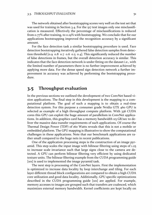
3.5. THROUGHPUT EVALUATION 51
The network obtained after bootstrapping scores very well on the test set that was used for training in Section 3.4. For the 517 test images only one misclassifi-cation is measured. Effectively the percentage of misclassifications is reduced from 0.77% after training, to 0.19% with bootstrapping. We conclude that for our applications bootstrapping improved the recognition accuracy by a significant amount.
For the face detection task a similar bootstrapping procedure is used. Face detection bootstrapping iteratively gathered false detection samples from detec-tion threshold [0.9 0.8 0.7 0.6 0.5 0.4]. This significantly reduced the number of false detections in frames, but the overall detection accuracy is similar. This indicates that the face detection network is under fitting on the dataset i.e., with the limited number of parameters there is no further improvement achieved by applying more data. For the dense speed sign detection network a further im-provement in accuracy was achieved by performing the bootstrapping proce-dure.
3.5 Throughput evaluation
In the previous sections we outlined the development of two ConvNet based vi-sion applications. The final step in this development is the mapping to a com-putational platform. The goal of such a mapping is to obtain a real-time detection system. For this purpose a consumer grade Nvidia GTX 460 GPU is selected as example of a high throughput compute platform. With 336 CUDA cores this GPU can exploit the huge amount of parallelism in ConvNet applica-tions. In addition, this graphics card has a memory bandwidth 115 GB/sec to de-liver the massive data transfer requirements of such applications. Of course the Thermal Design Power (TDP) of 160 Watts reveals that this is not a mobile or embedded platform. The GPU mapping is illustrative to show the computational challenges in these applications. Note that our benchmark applications are ra-ther small compared to the huge nets in recent publications.
One of the application processing steps is the construction of an image pyr-amid. This step scales the input image with bilinear filtering using steps of 1.25 to increase scale invariance such that large signs close to the camera are de-tected. A GPU can perform bilinear filtering very efficient by using dedicated texture units. The bilinear filtering example from the CUDA programming guide [101] is used to implemented the image pyramid task.
The next step is processing of the ConvNet layers. First the implementation is optimized to increase data locality by loop interchange and tiling. For each layer different thread block configurations are compared to obtain a high CUDA core utilization and good data locality. Additionally, GPU specific optimizations described in the CUDA programming guide [101] are applied. For example, memory accesses to images are grouped such that transfers are coalesced, which maximizes external memory bandwidth. Kernel coefficients are kept locally on
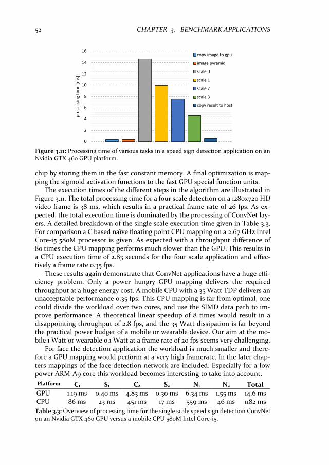
52 CHAPTER 3. BENCHMARK APPLICATIONS
chip by storing them in the fast constant memory. A final optimization is map-ping the sigmoid activation functions to the fast GPU special function units.
The execution times of the different steps in the algorithm are illustrated in Figure 3.11. The total processing time for a four scale detection on a 1280x720 HD video frame is 38 ms, which results in a practical frame rate of 26 fps. As ex-pected, the total execution time is dominated by the processing of ConvNet lay-ers. A detailed breakdown of the single scale execution time given in Table 3.3. For comparison a C based naïve floating point CPU mapping on a 2.67 GHz Intel Core-i5 580M processor is given. As expected with a throughput difference of 80 times the CPU mapping performs much slower than the GPU. This results in a CPU execution time of 2.83 seconds for the four scale application and effec-tively a frame rate 0.35 fps.
These results again demonstrate that ConvNet applications have a huge effi-ciency problem. Only a power hungry GPU mapping delivers the required throughput at a huge energy cost. A mobile CPU with a 35 Watt TDP delivers an unacceptable performance 0.35 fps. This CPU mapping is far from optimal, one could divide the workload over two cores, and use the SIMD data path to im-prove performance. A theoretical linear speedup of 8 times would result in a disappointing throughput of 2.8 fps, and the 35 Watt dissipation is far beyond the practical power budget of a mobile or wearable device. Our aim at the mo-bile 1 Watt or wearable 0.1 Watt at a frame rate of 20 fps seems very challenging.
For face the detection application the workload is much smaller and there-fore a GPU mapping would perform at a very high framerate. In the later chap-ters mappings of the face detection network are included. Especially for a low power ARM-A9 core this workload becomes interesting to take into account.
Table 3.3: Overview of processing time for the single scale speed sign detection ConvNet on an Nvidia GTX 460 GPU versus a mobile CPU 580M Intel Core-i5.
Platform C1 S1 C2 S2 N1 N2 Total
GPU 1.19 ms 0.40 ms 4.83 ms 0.30 ms 6.34 ms 1.55 ms 14.6 ms CPU 86 ms 23 ms 451 ms 17 ms 559 ms 46 ms 1182 ms
0
2
4
6
8
10
12
14
16
pro
cess
ing
tim
e [m
s]
copy image to gpu
image pyramid
scale 0
scale 1
scale 2
scale 3
copy result to host
Figure 3.11: Processing time of various tasks in a speed sign detection application on an Nvidia GTX 460 GPU platform.

3.6. RELATED WORK 53
3.6 Related work
This section will focus on other real-world vision applications that use a ConvNet for object detection and localization. Recently the computer vision community embraced ConvNets which is improving the state-of-the-art. It would have been great to use one of the recently proposed vision pipelines as a benchmark appli-cation. However, the mapping effort of these new applications would involve a substantial amount of work. We will see in this section that the main compute workload in these applications is not any different from our smaller benchmarks.
3.6.1 Region based convolutional networks
Our benchmark applications are designed for scenarios with were one type of object is localized in a frame. For example, the face detector generalizes such that many different types of faces (with glasses, facial hear, skin color, etc.) are detected. The speed sign recognizer detects a relatively small set of signs that all look very similar. Recently introduced vision applications have increased the complexity of detection and localization scenarios substantially. A very influen-tial paper (cited over 3400 times) on the use of ConvNets for object detection is the work on Region based ConvNets [55]. The region based ConvNets split the recognition task into a region proposal step and a classification step. Instead of searching the whole frame a selective search method [144] is used to obtain boxes or so called region proposals are selected based on texture, color, and intensity of neighboring pixels. These region proposals are suggestions for objects that are passed to a powerful classifier such as one of the ImageNet winners [79,142,138,62]. For each region proposal the following steps are performed:
1. Warp the content to a size fitted for the ConvNet patch size. 2. Compute the ConvNet layers up to the last classification layer. 3. Use a SVM classifier to identify the object. 4. Use a bounding box regressor to refine the proposal region.
The region based ConvNets successfully apply a large ConvNet as feature ex-tractor in a classical compute vision pipeline. Although the approach works re-ally well, it is computationally very demanding. About 2000 regions are generated per image that each require a forward pass through a large network. Furthermore, the training is demanding since three models are trained: A Conv-Net to generate image features; the classifier that predicts the class, the regres-sion model to refine the bounding boxes. To overcome the computational issues Fast Region ConvNets are introduced [54]. Instead of generating region pro-posals from the image, the feature map activations in a ConvNet layer are warped as proposals. The huge advantage is that the feedforward run is performed only once per image. The network input patch size is stretched to match the image size, which is far more efficient than evaluating all those proposal patches. In essence this approach is similar to our benchmarks where we also scale the net-work to use the full frame. However in this work they use the ConvNet features

54 CHAPTER 3. BENCHMARK APPLICATIONS
on which they perform Region of Interest (RoI) pooling. These features are warped into the proposal box that is the classification layer input. The final part of the model uses the RoI feature vector to perform classification with a SoftMax layer and a regressor for the bounding box refinement. The huge advantage is that this structure results in a single network model.
Fast region ConvNets provide a 25 times speedup over the original algorithm, but there is still a performance bottleneck. In a follow-up work so called Faster Region Proposal ConvNets [122] are introduced. These remove the selective search step. A new region proposal network is inserted after the last convolu-tional layer. It uses the raw feature maps to decide if there is an objects and pro-pose a box location. From that point onwards the same pipeline is used as for the fast region ConvNets. The faster region proposal ConvNets have increased throughput by 10 times over the fast region proposal networks. As a result this work is able to test images in about 0.2 seconds per frame. Note that this is a GPU accelerated throughput 0f 5 fps, performed by an NVIDIA Tesla K45 that consumes about 235 Watt of power under load conditions. Unless the huge effi-ciency improvements that are recently demonstrated it seems that region pro-posal ConvNets are computationally still way too demanding for real-time applications on embedded devices. However, we should mention here that re-gion proposal ConvNets are more accurate and much more general purpose in classification compared to our benchmarks.
3.6.2 Single shot detectors
A more efficient approach to object detection are the recently introduced Single Shot Detectors. These perform object detection as a single regression problem, directly from pixels to bounding box coordinates and class probabilities. A key
Figure 3.12: The output of a single shot detector like the YOLO model. The image is rep-resented as an S x S grid, each cell is encoded as a vector that contains class probabilities and the confidence for different bounding boxes. Image source: [86].

3.7. CONCLUSIONS AND DISCUSSION 55
system that adopts this approach is named You Only Look Once (YOLO) [121]. They train a single network to segment an image into a low resolution grid, see Figure 3.12. Each cell in the grid contains a vector with the probability to be one of the 20 object classes, and two bounding boxes definitions (xpos, ypos, width, height, confidence). To filter out the final box positions a Non-Maxima Suppres-sion algorithm is used as a post-processing step. The base YOLO model requires input images of 448x448 pixels and performs the detections in real-time at 45 frames per second. This is almost a 10 times increase compared to the Faster Region Proposal ConvNets. Note that the YOLO model uses less object classes and it is constrained in the box positioning and sizing accuracy. The 45 fps throughput is achieved on a NVIDIA Titan X GPU that consumes about 250 Watts of power under load.
Very recently, the concepts of the single shot YOLO approach are further improved as described in the Single Shot MultiBox Detector (SSD) work [89]. To improve the detection accuracy SSD uses feature maps of different scales, and they explicitly separate predictions by aspect ratio. For training they use ad-vanced data augmentation techniques, like hard negative mining which is essen-tially similar to iterative bootstrapping see section 3.4.4. The sampling of training examples is performed under special conditions to improve detection accuracy, e.g. object boxes with less overlap or the wrong aspect rations. The SSD on a 300x300 pixel image is with 46 fps slightly faster than the 448x448 pixel YOLO approach. Both use a NVIDIA Titan X GPU. The main improvement of the SSD is the substantially better accuracy which is on-par with the much slower region proposal methods.
The compute workload in Single Shot Detector is very similar to the workload in our benchmark applications. The techniques proposed in this thesis can bring further efficiency improvements to enable the use of ConvNet based object de-tection on power constrained embedded devices. This to replace the 250Watt power hungry GPU by a low power (≤ 1 Watt) embedded device.
3.7 Conclusions and discussion
In this chapter we demonstrate how a ConvNet based vision application is de-veloped. We have shown the large computational differences between a single patch classification ConvNet and a multiscale video detection application that embeds a ConvNet. Furthermore, the importance of training data collection is emphasized. A good training and validation set is essential in the development of vision applications that performs well in a real-world environment. Addition-ally, the dataset should be used in a network training procedure to obtain a set of network parameters that solves the recognition problem. Training a ConvNet is a very demanding task, but often this is a one-time effort that can be done in a lab. Although this thesis focuses on inference and not on the training task, we

56 CHAPTER 3. BENCHMARK APPLICATIONS
show that during training the network structure should be adapted to substan-tially improve the efficiency for the inference workload. For example our speed sign detection workload can be reduced by a factor 2.3 without loss of quality.
Our application development efforts resulted in two ConvNet applications that are used through the next chapters of this thesis. One is a Speed Sign Detec-tion application for driver assistance or autonomous driving. The other applica-tion performs Face Detection for surveillance. Both video applications are very representative examples of deep learning based machine vision applications that will be deployed in the very near future as replacements of classical model based object recognition systems. The more advanced state-of-the-art detection and localization works often use a different training approach, but except for the post processing the inference mode is very similar to our benchmark networks. At this point we conclude that for a wide range of ConvNet structures our applica-tions are quite representative. The face detection workload is a very sparse ex-ample where the speed sign network contains a quite dense workload.
By mapping the Speed Sign detection ConvNet to an NVidia Graphics Pro-cessing Unit (GPU) we demonstrated that our workload is very suitable for par-allel compute platforms. Furthermore this mapping demonstrates that real-time detection tasks by ConvNet based vision applications is possible. However the 160 Watt power consumption for this GPU is far above the mobile energy budget. Another mapping to a mobile CPU shows a disappointing 0.35 fps throughput, and also this platform consumes a factor 35 more power than allowed. These mapping reveal the huge compute efficiency problem in ConvNet application workloads.
To harvest the huge advantages of deep learning based applications for our mobile devices the efficiency problems must be solved. The remainder of this thesis will focus on reducing the workload and improving the compute efficiency of these applications. If we could bring the deep learning techniques to our em-bedded platforms it will open a whole domain of new application opportunities. Firstly, the deep learning base applications have shown to outperform classical approaches in classification quality, for some problems superhuman perfor-mance is demonstrated. Secondly, application features can be added by a simple coefficient file update. Or our applications can automatically learn from errors made in a real-wold environment. These possibilities will greatly improve the quality of the next generation of machine vision applications.

57
4.
ALGORITHMIC OPTIMIZATIONS
The huge computational requirements of Convolutional Networks (Conv-Nets) often reduce their applicability to offline detection tasks. To ease these requirements we propose a high-level algorithmic modification appli-cable to the first layers of a ConvNet. These first layers are responsible for feature extraction by alternating Convolution and Pooling layers. This first part is often very complicated with multiple layers that often contain over 100,000 interconnected computational nodes. The proposed modification reduces computational complexity; real benchmarks show 65 - 83% reduc-tion, with equal recognition accuracy. Often such modifications can intro-duce severe implications to the available parallelism. Therefore, the modified CNN algorithm is implemented and evaluated on a GPU platform to demonstrate the suitability of the proposed modification for massively parallel platforms. Our benchmark implementation achieves a speedup of 2.5 times w.r.t. the original algorithm. This chapter is based on work presented in ACIVS 2011 [103]
4.1 Introduction
Although Deep Convolutional Networks (ConvNets) achieve the best accuracy on many vision or classification tasks they are rarely used in mobile or embedded applications. In the earlier chapters we motivated that the huge computational challenges in (ConvNets) often prevent their usage in embedded systems. Often there exist a less accurate, but computationally cheaper algorithm. In these sce-narios a classical model based solution is often used that trades functionality, accuracy, and robustness to obtain a simpler algorithm. Our main goal is to im-prove the efficiency of ConvNets, such that this class of algorithms with all their desirable properties can be used in mobile applications. In this first optimization chapter we focus on reducing the computational complexity without sacrificing on accuracy or quality.
CHAPTER

58 CHAPTER 4. ALGORITHMIC OPTIMIZATION
ConvNets have many levels of possible improvements e.g., Algorithmic, Til-ing and Memory, Platform Architecture, and Technology. Here we focus on al-gorithmic changes, these are more abstract and can have a huge impact on the performance. A successful example is the 3-D RS motion estimator [41] that im-proved the expensive full-search block matchers into smart efficient recursive matchers. This algorithmic optimization is very radical and almost a different algorithm. However, in essence it still matches the surrounding blocks to find a best candidate for the motion vector.
In our work a modified feature extraction stage for ConvNets is proposed that reduces the computational workload and the number of data transfers. Figure 4.1 illustrates the feature extraction part that we optimize. Note that our optimi-zation does not apply to the classification stage. The optimization can be directly applied on a trained networks. However, it is also possible to train a ConvNet structure with this modification, so we derived the required training rules. The network accuracy after training is evaluated with two real world benchmarks. To verify the theoretical performance claims, an Intel CPU and an NVIDIA CUDA-enabled Graphics Processing Unit (GPU) mapping is performed to demonstrate the achieved performance improvement.
The remainder of this chapter is organized as follows. Section 4.2 contains a recap of the ConvNet model to explain the proposed optimization. Then section 4.3 describes the algorithmic optimization and new training rules are derived. Next, section 4.4 evaluates the recognition accuracy of the optimization. Section 4.5 describes our mapping of the feature extractors and the speedup of our mod-ification is evaluated. Related work and Conclusion are presented in Section 4.6 and 4.7 respectively.
4.2 Feature extraction layers
To explain the proposed algorithmic modifications, we provide a short recap the feature extraction part of a ConvNet. More details on the algorithm are discussed in Chapter 2.
input32 x 32
feature maps28 x 28
5x5convolution
2x2pooling
feature maps14 x 14
feature maps10 x 10
feature maps5 x 5
5x5convolution 2x2
poolingfully
connected
C1 P1 C2 P2 n1 n2
output
feature extraction classification
01
89
Figure 4.1: An example CNN architecture used for a handwritten digit recognition task.

4.2. FEATURE EXTRACTION LAYERS 59
Although ConvNets have different configurations with many or a few layers they often have a similar structure to the network depicted in Figure 4.1. Their first layers function as trainable feature extractor, and the second part imple-ments a classifier. These first layers have constraints like receptive fields and weight sharing to extract position invariant features from two-dimensional shapes. Many networks contain two different successive layer types to extract these features: Convolution Layers, and Pooling Layers.
4.2.1 Convolution layers
In Figure 4.1 layers C1 and C2 are convolution layers. They take inputs from a local receptive field, and all neighboring neurons share the same set of weights. Basi-cally it is a similar operation as a convolution by a small weight kernel. The 2d or 3d operation in a convolution layer that generates a single feature map is de-fined as:
𝑐[𝑚, 𝑛] = 𝜑(𝑝) = 𝜑(𝑏 +∑ ∑ 𝑤𝑞[𝑘, 𝑙] 𝑥𝑞[𝑚 + 𝑘, 𝑛 + 𝑙]
𝐾−1
𝑘,𝑙=0𝑞∈𝑄
) (4.1)
Here 𝑏 is the bias, 𝑤 the shared weight kernel, and 𝑥 is an input feature map that is transformed into output feature map 𝑐. The outer sum over 𝑞 is optional, in layer C2 it is used to sum the contributions of multiple input feature maps. Dif-ferent activation function 𝜑 can be used, in chapter 1 we discussed several op-tions.
4.2.2 Pooling layers
As depicted in Figure 4.1 most convolution layers are succeeded by a pooling layer (P1 and P2) to reduce the number of detected features. There are two pop-ular pooling functions that reduce the number of features.
1) Subsampling summarizes a window of features by local averaging with a trainable coefficient and a bias offset. The subsampling operation is defined as:
𝑦[𝑚, 𝑛] = 𝜑(𝑝) = 𝜑 (𝑎 + 𝑣 ∑ 𝑥[𝑚𝑆 + 𝑘, 𝑛𝑆 + 𝑙]
𝑆−1
𝑘,𝑙=0
) (4.2)
Here 𝑣 and 𝑎 are trainable parameter for scaling and bias offset respectively. 2) Max pooling, selects the local maximum from a window.
𝑦[𝑚, 𝑛] = 𝜑(𝑝) = 𝜑 ( max0≤𝑘<𝑆,0≤𝑙<𝑆
(𝑥[𝑚𝑆 + 𝑘, 𝑛𝑆 + 𝑙])) (4.3)
Both function use scale factor 𝑆 as reduction parameter. These reduction param-eters define the distance between neighboring windows. Note that a window can have overlap.

60 CHAPTER 4. ALGORITHMIC OPTIMIZATION
4.3 Algorithm optimization
In the previous section the feature extraction layers of a ConvNet are outlined. Depending on the network configuration these first layers will be responsible for a significant up to a large portion of the computational workload. The optimiza-tion proposed in this section focuses on reducing the workload in these first lay-ers by merging the operation of convolution and pooling into a single operation. Depending on the network configuration there are two scenarios when our op-timization is applied be applied:
1) A trained ConvNet can be directly converted into an optimized net if there is a linear function from the convolution layer inputs to the pooling layer. For example, conversion is possible when the convolution layer does not use an ac-tivation function and the pooling function performs subsampling.
2) A ConvNet must be retrained after conversion to the optimized network. This is necessary when a non-linear activation function is used in the convolu-tion layer, or when the subsampling layer uses max-pooling.
4.3.1 Merge convolution and pooling
The merge operation of convolution and pooling layers can be derived from de-pendency analysis. Figure 4.2 illustrates the data dependencies between both layers; it also shows how a single operation could bypass the convolution result. In the scenario of direct merging a new operator is obtained by substitution of the convolution operation (4.1) into the subsample expression (4.2). This substi-tution of operations is outlined in equation (4.4). The new enlarged kernel �̃� is constructed from all coefficients that are multiplied by each input 𝑥. The new
bias �̃� is the convolution layer bias 𝑏 multiplied by 𝑣 and summed with the sub-sample bias 𝑎.
inputX
poolingY
convolutionC
S2·K2
kernel
(K+S-1)2
kernel
S2
kernel
Figure 4.2: Dependency analysis for a 2d-convoluiton kernel of size 𝑲 = 𝟑 and pooling layer where 𝑺 = 𝟐. The dependencies from the input to convolution layer are given in red these results are consumed by the pooling layer. The merged solution directly consumes the inputs to generate the pooling result.
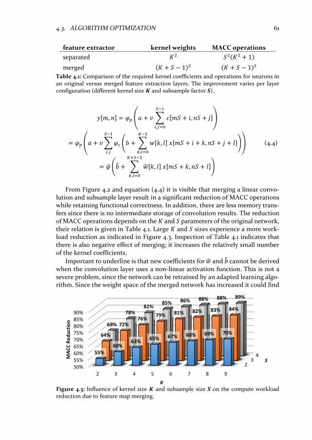
4.3. ALGORITHM OPTIMIZATION 61
From Figure 4.2 and equation (4.4) it is visible that merging a linear convo-lution and subsample layer result in a significant reduction of MACC operations while retaining functional correctness. In addition, there are less memory trans-fers since there is no intermediate storage of convolution results. The reduction of MACC operations depends on the 𝐾 and 𝑆 parameters of the original network, their relation is given in Table 4.1. Large 𝐾 and 𝑆 sizes experience a more work-load reduction as indicated in Figure 4.3. Inspection of Table 4.1 indicates that there is also negative effect of merging; it increases the relatively small number of the kernel coefficients.
Important to underline is that new coefficients for �̃� and �̃� cannot be derived when the convolution layer uses a non-linear activation function. This is not a severe problem, since the network can be retrained by an adapted learning algo-rithm. Since the weight space of the merged network has increased it could find
feature extractor kernel weights MACC operations
separated 𝐾2 𝑆2(𝐾2 + 1)
merged (𝐾 + 𝑆 − 1)2 (𝐾 + 𝑆 − 1)2
𝑦[𝑚, 𝑛] = 𝜑𝑝 (𝑎 + 𝑣 ∑ 𝑐[𝑚𝑆 + 𝑖, 𝑛𝑆 + 𝑗]
𝑆−1
𝑖,𝑗=0
)
= 𝜑𝑝 (𝑎 + 𝑣∑𝜑𝑐 (𝑏 + ∑ 𝑤[𝑘, 𝑙] 𝑥[𝑚𝑆 + 𝑖 + 𝑘, 𝑛𝑆 + 𝑗 + 𝑙]
𝐾−1
𝑘,𝑙=0
)
𝑆−1
𝑖,𝑗
) (4.4)
= �̃� (�̃� + ∑ �̃�[𝑘, 𝑙] 𝑥[𝑚𝑆 + 𝑘, 𝑛𝑆 + 𝑙]
𝐾+𝑆−2
𝑘,𝑙=0
)
Table 4.1: Comparison of the required kernel coefficients and operations for neurons in an original versus merged feature extraction layers. The improvement varies per layer configuration (different kernel size 𝑲 and subsample factor 𝑺).
23
4
50%55%60%65%70%75%80%85%90%
2 3 4 5 6 7 8 9
55%60%
63%65% 67% 68% 69% 70%64%
72%76%
79% 81% 82% 83% 84%
69%
78%82%
85% 86% 88% 88% 89%
S
MA
CC
Re
du
ctio
n
KFigure 4.3: Influence of kernel size 𝑲 and subsample size 𝑺 on the compute workload reduction due to feature map merging.
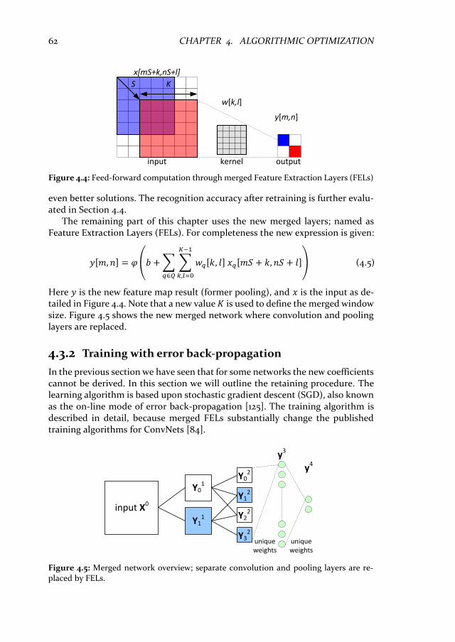
62 CHAPTER 4. ALGORITHMIC OPTIMIZATION
even better solutions. The recognition accuracy after retraining is further evalu-ated in Section 4.4.
The remaining part of this chapter uses the new merged layers; named as Feature Extraction Layers (FELs). For completeness the new expression is given:
𝑦[𝑚, 𝑛] = 𝜑(𝑏 +∑ ∑ 𝑤𝑞[𝑘, 𝑙] 𝑥𝑞[𝑚𝑆 + 𝑘, 𝑛𝑆 + 𝑙]
𝐾−1
𝑘,𝑙=0𝑞∈𝑄
) (4.5)
Here 𝑦 is the new feature map result (former pooling), and 𝑥 is the input as de-tailed in Figure 4.4. Note that a new value 𝐾 is used to define the merged window size. Figure 4.5 shows the new merged network where convolution and pooling layers are replaced.
4.3.2 Training with error back-propagation
In the previous section we have seen that for some networks the new coefficients cannot be derived. In this section we will outline the retaining procedure. The learning algorithm is based upon stochastic gradient descent (SGD), also known as the on-line mode of error back-propagation [125]. The training algorithm is described in detail, because merged FELs substantially change the published training algorithms for ConvNets [84].
x[mS+k,nS+l]
y[m,n]
S K
w[k,l]
input kernel output
Figure 4.4: Feed-forward computation through merged Feature Extraction Layers (FELs)
input X0
Y01
Y11
Y02
Y12
Y22
Y32
y3
y4
unique weights
unique weights
Figure 4.5: Merged network overview; separate convolution and pooling layers are re-placed by FELs.

4.3. ALGORITHM OPTIMIZATION 63
In chapter 2 the Stochastic Gradient Descent (SGD) algorithm is introduced. Here we explain the modifications that are necessary to apply SGD on ConvNets with merged FELs. The basic idea does not change; again partial derivatives of the error in function of the weights are computed for a given input pattern. These derivatives are used to reduce the error by small weight updates in the negative direction of the derivative. For clarity this procedure is split in three parts; feed-forward processing, partial derivative computation, and weight up-dates. During the outline of the algorithm we use the notation given in Figure 4.4 to describe signals in different layers.
Feed-forward processing
Before training all coefficients are initialized to a small random value. First a pattern from the training set is processed in feed-forward by the merged Conv-Net, using equation (4.5) for the FELs and a regular multi-layer perceptron (1.8) for the classification part. Next, the network outputs are compared with the de-sired output in an error-function. In this case we used the cross-entropy error function [64] as given in equation (4.6). Here 𝑁 is the set output neurons, 𝑑𝑛 the target labels, and 𝑦𝑛 the output neuron values.
𝐸CE = − ∑ 𝑑𝑛 log(𝑦𝑛) + (1 − 𝑑𝑛) log(1 − 𝑦𝑛)
∀𝑛∈𝑁
(4.6)
Compute partial derivatives
The previous expressions us 𝑥 for layer inputs and 𝑦 for outputs. The back prop-
agation of derivatives over layers requires more variables, so we use 𝑦𝜆 to specify from which relative layer we obtain inputs. We start computing local gradients from the output of the network towards the input. This is done by applying the chain rule on the cross-entropy error function, which results in:
𝜕𝐸CE
𝜕𝑤𝑛𝜆[𝑘]
=𝜕𝐸CE
𝜕𝑦𝑛𝜆 𝜕𝑦𝑛
𝜆
𝜕𝑝𝑛𝜆 𝜕𝑝𝑛
𝜆
𝜕𝑤𝑛𝜆[𝑘]
=𝑦𝑛𝜆 − 𝑑𝑛
𝑦𝑛𝜆(1 − 𝑦𝑛
𝜆) 𝜑′(𝑝𝑛
𝜆) 𝑦𝑘𝜆−1 (4.7)
= (𝑦𝑛𝜆 − 𝑑𝑛) 𝑦𝑘
𝜆−1
= 𝛿𝑛𝜆 𝑦𝑘
𝜆−1
Important for the simplification is:
𝜑′(𝑥) = 𝜑(𝑥)(1 − 𝜑(𝑥)) = 𝑦𝑛(1 − 𝑦𝑛) (4.8)
𝛿 =𝜕𝐸CE𝜕𝑦
𝜕𝑦
𝜕𝑝 (4.9)
Efficient computation of partial derivatives for the non-output neuron layers can be done by reusing the local gradients 𝛿 of the output layer.
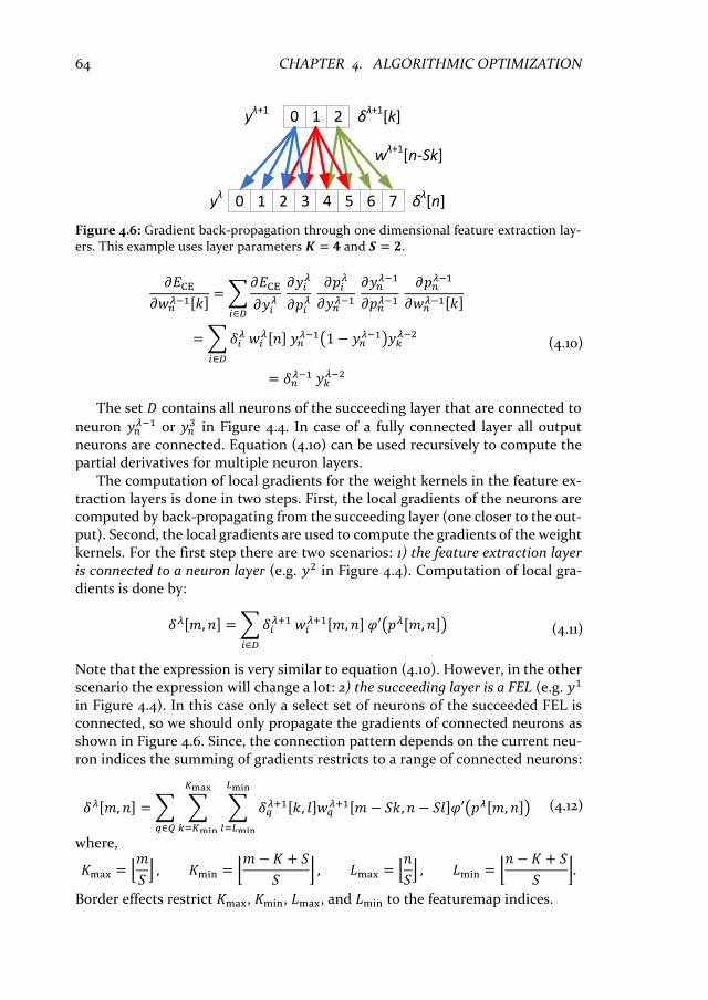
64 CHAPTER 4. ALGORITHMIC OPTIMIZATION
𝜕𝐸CE
𝜕𝑤𝑛𝜆−1[𝑘]
=∑𝜕𝐸CE
𝜕𝑦𝑖𝜆 𝜕𝑦𝑖
𝜆
𝜕𝑝𝑖𝜆 𝜕𝑝𝑖
𝜆
𝜕𝑦𝑛𝜆−1
𝑖∈𝐷
𝜕𝑦𝑛𝜆−1
𝜕𝑝𝑛𝜆−1
𝜕𝑝𝑛
𝜆−1
𝜕𝑤𝑛𝜆−1[𝑘]
=∑𝛿𝑖𝜆 𝑤𝑖
𝜆[𝑛] 𝑦𝑛𝜆−1(1 − 𝑦𝑛
𝜆−1)𝑦𝑘𝜆−2
𝑖∈𝐷
(4.10)
= 𝛿𝑛𝜆−1 𝑦𝑘
𝜆−2
The set 𝐷 contains all neurons of the succeeding layer that are connected to
neuron 𝑦𝑛𝜆−1 or 𝑦𝑛
3 in Figure 4.4. In case of a fully connected layer all output neurons are connected. Equation (4.10) can be used recursively to compute the partial derivatives for multiple neuron layers.
The computation of local gradients for the weight kernels in the feature ex-traction layers is done in two steps. First, the local gradients of the neurons are computed by back-propagating from the succeeding layer (one closer to the out-put). Second, the local gradients are used to compute the gradients of the weight kernels. For the first step there are two scenarios: 1) the feature extraction layer is connected to a neuron layer (e.g. 𝑦2 in Figure 4.4). Computation of local gra-dients is done by:
𝛿𝜆[𝑚, 𝑛] = ∑𝛿𝑖𝜆+1 𝑤𝑖
𝜆+1[𝑚, 𝑛] 𝜑′(𝑝𝜆[𝑚, 𝑛])
𝑖∈𝐷
(4.11)
Note that the expression is very similar to equation (4.10). However, in the other scenario the expression will change a lot: 2) the succeeding layer is a FEL (e.g. 𝑦1 in Figure 4.4). In this case only a select set of neurons of the succeeded FEL is connected, so we should only propagate the gradients of connected neurons as shown in Figure 4.6. Since, the connection pattern depends on the current neu-ron indices the summing of gradients restricts to a range of connected neurons:
𝛿𝜆[𝑚, 𝑛] = ∑ ∑ ∑ 𝛿𝑞𝜆+1[𝑘, 𝑙]𝑤𝑞
𝜆+1[𝑚 − 𝑆𝑘, 𝑛 − 𝑆𝑙]𝜑′(𝑝𝜆[𝑚, 𝑛])
𝐿min
𝑙=𝐿min
𝐾max
𝑘=𝐾min𝑞∈𝑄
(4.12)
where,
𝐾max = ⌊𝑚
𝑆⌋ , 𝐾min = ⌊
𝑚 − 𝐾 + 𝑆
𝑆⌋ , 𝐿max = ⌊
𝑛
𝑆⌋ , 𝐿min = ⌊
𝑛 − 𝐾 + 𝑆
𝑆⌋.
Border effects restrict 𝐾max, 𝐾min, 𝐿max, and 𝐿min to the featuremap indices.
δλ[n] 0 1 2 3 4 5
0 1
6 7
2
wλ+1[n-Sk]
δλ+1[k]
yλ
yλ+1
Figure 4.6: Gradient back-propagation through one dimensional feature extraction lay-ers. This example uses layer parameters 𝑲 = 𝟒 and 𝑺 = 𝟐.

4.4. EVALUATE RECOGNITION PERFORMANCE 65
In the second step, the local neuron gradients are used to compute the gra-dients of FEL coefficients. Since, the bias is connected to all feature map neurons we obtain its gradient by summing over the local gradients:
𝜕𝐸CE𝜕𝑏
= ∑ 𝛿[𝑚, 𝑛 ]0≤ 𝑚 < 𝑀0≤𝑛<𝑁
(4.13)
The gradients for the kernel coefficients are obtained by:
𝜕𝐸CE
𝜕𝑤𝜆[𝑘, 𝑙]= ∑ 𝛿𝜆[𝑚, 𝑛] 𝑦𝜆−1[𝑚𝑆 + 𝑘, 𝑛𝑆 + 𝑙]
0≤ 𝑚 < 𝑀0≤𝑛<𝑁
(4.14)
Update network coefficients
The standard delta rule for SGD is used for updating to keep training simple and reproducible with 𝜂 as single tuning parameter. This well-known coefficient up-date function uses the computed gradients to push the weights to a better solu-tion.
𝑊new = 𝑊old − 𝜂𝜕𝐸CE𝜕𝑊old
(4.15)
In the update function (4.15) 𝑊 refers to all weigths 𝑤 and bias 𝑏 values in the network.
4.4 Evaluate recognition performance
In the previous section we introduced merging of convolution and pooling layers to reduce computational workload. If a ConvNet uses max-pooling or the con-volution layer has a non-linear activation function the network must be retained to obtain a new coefficient set. In this section we evaluate the recognition accu-racy after merging and retraining. Obviously, in case direct computation of the weights is possible there is no difference in accuracy.
To evaluate the recognition performance we use two well-known data sets with known network configurations, which increases reproducibility. The first evaluation is done on the MNIST handwritten digit dataset [84]. MNIST consists of 70.000 samples, each containing a 28x28 pixel digit as shown in Figure 4.7a. We use the LeNet-5 ConvNet to compare separated versus merged accuracy [84]. The second dataset is the small-NORB object classification dataset [85]. NORB consist of 48,600 stereoscopic image pairs, each 96x96 pixels as shown in Figure 4.7b. This set contains 50 different objects from different angles, distributed over 5 classes. For evaluation we use the LeNet-7 network, which is substantially larger compared to LeNet5. For training we used our MATLAB implementation of both networks and our implementation of the SGD training algorithm. As in the benchmark papers we used the original dataset division: MNIST 60,000 for
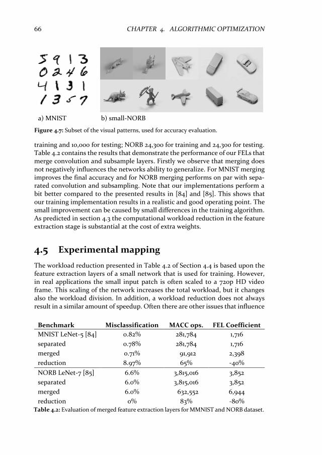
66 CHAPTER 4. ALGORITHMIC OPTIMIZATION
training and 10,000 for testing; NORB 24,300 for training and 24,300 for testing. Table 4.2 contains the results that demonstrate the performance of our FELs that merge convolution and subsample layers. Firstly we observe that merging does not negatively influences the networks ability to generalize. For MNIST merging improves the final accuracy and for NORB merging performs on par with sepa-rated convolution and subsampling. Note that our implementations perform a bit better compared to the presented results in [84] and [85]. This shows that our training implementation results in a realistic and good operating point. The small improvement can be caused by small differences in the training algorithm. As predicted in section 4.3 the computational workload reduction in the feature extraction stage is substantial at the cost of extra weights.
4.5 Experimental mapping
The workload reduction presented in Table 4.2 of Section 4.4 is based upon the feature extraction layers of a small network that is used for training. However, in real applications the small input patch is often scaled to a 720p HD video frame. This scaling of the network increases the total workload, but it changes also the workload division. In addition, a workload reduction does not always result in a similar amount of speedup. Often there are other issues that influence
Table 4.2: Evaluation of merged feature extraction layers for MMNIST and NORB dataset.
Benchmark Misclassification MACC ops. FEL Coefficient
MNIST LeNet-5 [84] 0.82% 281,784 1,716
separated 0.78% 281,784 1,716
merged 0.71% 91,912 2,398
reduction 8.97% 65% -40%
NORB LeNet-7 [85] 6.6% 3,815,016 3,852
separated 6.0% 3,815,016 3,852
merged 6.0% 632,552 6,944
reduction 0% 83% -80%
a) MNIST b) small-NORB
Figure 4.7: Subset of the visual patterns, used for accuracy evaluation.

4.5. EXPERIMENTAL MAPPING 67
the speedup e.g., the memory behavior (cache misses), or the utilized parallel-ism. To quantify the real speedup we mapped our speed sign recognition appli-cation with merged FELs to a CPU and a GPU. These mapping results are compared to the results we presented in Chapter 3 to obtain a quantitative meas-ure of speedup.
First a single core C implementation is developed for a 2.66 GHz Intel Core-i5 M580 processor. This mapping is optimized for data locality by loop inter-changes. The code is compiled with MS Visual Studio 2010 where the compiler flags are set to optimize for execution speed.
Secondly, a massively parallel implementation is developed for an NVIDIA GTX460 GPU platform. Feature extraction layers contain a lot of parallelism, so a good speedup is expected. For fair comparison of the feature extraction layers we tuned the code to utilize the GPU thread parallelism and to improve data locality (loop interchanges and tiling). In addition, GPU specific optimizations described in the CUDA programming guide [101] are applied. For example, memory accesses to the images and feature-maps are grouped to enforce fast coalesced memory accesses. The kernel coefficients are stored in fast constant memory. As final optimization the non-linear sigmoid activation function is evaluated fast using the special function units on the GPU. To enable this last optimization specific intrinsics from the programming guide are used:
__fdividef(1,1+__expf(-x));
The execution times for the CPU and GPU mappings are presented in Table 4.3. The speed sign application uses window size 𝐾 = 5 and subsample factor 𝑆 = 2, so according to Figure 4.3 there should be a workload reduction of 65%. This workload reduction is very much in line with the 2.84 times speedup that is demonstrated on the CPU platform. For the sequential case we demonstrated an effective speedup similar to the workload reduction. However for the parallel platform this is not entirely true. Although the speedup of 2.48 times is consid-ered as quite good, it is 13% less than the theoretical improvement. A parallel mapping of merged layers has more complicated access patterns and it utilizes less data reuse; both make that the theoretical speedup is not achieved. Still it is important to underline that our merged feature extractors improve the real GPU implementation by 2.48 times, which is a substantial speedup.
Table 4.3: Speed sign recognition application execution time comparison of separated versus merged feature extraction stage.
configuration CPU GPU speedup
separate conv. & sub. 577 ms 6.72 ms 86 x
merged FELs 203 ms 2.71 ms 75 x
speedup 2.84 x 2.48 x
68 CHAPTER 4. ALGORITHMIC OPTIMIZATION
4.6 Related work
Improving the throughput of ConvNets is not a new field of research. In the last decade many works proposed dedicated hardware implementations and accel-erators for ConvNets [16,51]. These implementations often reduce execution time by the use of hand crafted systolic implementations of the convolution opera-tion, which heavily reduces the flexibility. For example, a 3x3 convolution per-formed by a systolic 10x10 array results in a utilization of only 9% of the multipliers.
Improving the throughput by algorithmic optimization is often much more flexible and it can be applied to multiple platforms. For example, a related accel-eration approach was presented in [137], where the authors give a reduced type of ConvNet. Instead of averaging with subsampling by using equation (4.2) they only compute one of the convolution results in an 𝑆2 window. Similar to our approach this reduces computational complexity, however the number of net-work parameters is not increased. The paper does not report on any quality loss, but this could occur if one only reduces the number of operations. Furthermore, the work in [137] differs because there is no analysis published that shows how kernel size 𝐾 and pooling factor 𝑆 influence the reduction of computational complexity. Finally, there are no performance measurements on parallel plat-forms such as a GPU.
Nowadays it is evident that the excessive workload of ConvNets poses huge challenges for computing platforms. As a result multiple recent works on algo-rithmic optimization are published. For example, the well-known Strassen algo-rithm for efficient matrix multiplication is used to reduce the multiplication workload in ConvNets [36]. To enable this optimization series of input images is buffered (a batch). This creates an opportunity to rewrite a ConvNet as a Con-volutional Matrix Multiplication for which many optimized mappings are exist from the linear algebra domain. Although the theoretical workload reduction of 65% is substantial, the average measured runtime reduction of 17% is minimal. The main cause of this gap is because the technique trades multiplications for additions. This tradeoff could also result in more memory accesses due to the partial results that must be computed, and they must buffer a series of input frames. Instead of mobile accelerators, datacenters could be an excellent domain to apply the Convolutional Matrix Multiplication. However, their technique is not evaluated on a parallel platform, so for parallel scalability further research is required.
A similar but more refined optimization uses Winograd’s algorithm for min-imal filtering [81]. Their minimal filtering is able to reduce the multiplications without creating excessive overhead. CPU mappings demonstrate a 2.58 times speedup, and GPU mappings give a 2.26x speedup compared to direct imple-mentation. This complicated technique is highly tuned for 3x3 filter sizes, which give a very efficient Winograd transform. For larger kernel sizes such as 5x5 the

4.7. CONCLUSION 69
transform costs increase quickly and will overwhelm any savings in the number of multiplications.
Another high-level optimization approach performs convolutions in the fre-quency domain [145]. In frequency domain convolutions are point wise multipli-cations and therefor much cheaper compared to spatial domain. However, for small convolution kernels and small batch sizes the transformation costs destroy the savings in the number of multiplications. A combination of the Winograd and Frequency transform would probably give very competitive results.
A closely related work [75] also exploits the redundancies in representations that occur in ConvNet layers. They approximate the 2d convolution filters as combinations of a rank-1 filter basis (separable filters). Direct training a network on their rank-1 filter banks does not give good results. As a result, their approach requires an additional optimization on a trained network to find the optimal filter approximations. They report 2.4 times speedup without loss of accuracy. Their method also allows more accuracy loss e.g., at 1% accuracy loss they show 4x speedup.
Very recent work demonstrated that the weights in a deep ConvNet can be reduced to 1 bit (representing +1, or -1) with a scale factor 𝛼 per kernel [120]. In essence this convolution approximation is similar to the rank-1 filters of [75] but theirs is reduced even further. This so called Binary Weight Network must be trained with a custom implementation of SGD, and is able to achieve on-par performance with AlexNet [79]. However, on other large networks [142] a rela-tively large accuracy penalty of 5-10% is reported. The authors of [120] reduce the precision further by XNOR networks that additionally enforces the inputs of convolutions to 1 bit values (+1, or -1). XNOR nets use a trained scale matrix 𝛽𝑖,𝑗
for all outputs, and the 𝛼 scale per weight kernel. The XNOR approximates con-volutions with less parameters than the Binary Weight Network. As a result, the accuracy penalty on AlexNet [79] is 5-10%, and for GoogLenet [142] it does not converge anymore. Both Binary Weight Networks and XNOR exploit the param-eter redundancy in ConvNets to the extreme. As a result both substantially re-duce the memory footprint. Although throughput measurements for real network are not given we do expect a significant speedup due the this approxi-mation.
4.7 Conclusion
In this chapter a high-level algorithm modification is proposed to reduce the computational workload of the trainable feature extractors in a ConvNet. We demonstrated that the learning abilities of the modified algorithm did not de-crease; this is verified with real-world benchmarks. Our benchmarks show that the proposed modifications result in a MACC operation reduction of 65-83% for the required number of MACC operations in feature extraction layers.
To measure the actual application speedup due to workload reduction; our road sign classification application from Chapter 3 is used. This application is

70 CHAPTER 4. ALGORITHMIC OPTIMIZATION
mapped to a CPU and GPU platform. The speedup on CPU is a factor 2.7 where GPU implementation gains a factor 2.5, compared to the original convolution and subsample feature extractor. These speedups demonstrate that our modifi-cation is suitable for parallel implementation.
The modifications proposed in this chapter reduce the huge performance gap between the requirements of current ConvNets and the capabilities of todays embedded platforms. Although the factor 2.5-2.7 is not enough to close the per-formance gap it is a significant improvement that can be combined with other optimizations. In the next chapters we continue with different optimizations that use incorporate this layer merging technique.

71
5.
INTER-TILE REUSE OPTIMIZATION
Dedicated hardware acceleration of Convolutional Networks (ConvNets) can give a huge efficiency improvement over general purpose CPUs. A com-plex scaling problem that remains is the data transfer bottleneck. To scale-up performance accelerators require huge amounts of data, and often they are limited by interconnect resources. In addition, the energy spend by the accelerator is dominated by the transfer of data, either in the form of memory references or data movement over the interconnect. In this chapter we drastically reduce accelerator communication by exploration of compu-tation reordering and local scratchpad memory usage. Consequently, we present a new analytical methodology to optimize nested loops for inter-tile data reuse with loop transformations like interchange and tiling. We focus on embedded accelerators that can be used in a multi-accelerator System on Chip (SoC), so performance, area, and energy are key in this exploration. 1) We demonstrate that our methodology reduces external memory com-munication up to 2.1 times compared to the best case of intra-tile optimiza-tion. This is done on our Speed Sign ConvNet and two common embedded image/video processing workloads (demosaicing and block matching). 2) We demonstrate that our small accelerators (1-3% FPGA resources) can boost a simple Microblaze soft-core to the performance level of a high-end Intel-i7 processor. This chapter is based on work presented in ICCD 2013 [108] and DATE 2015 [104]
5.1 Introduction
For many algorithms the compute efficiency is improved orders of magnitude by using specialized hardware accelerators instead of general purpose processor cores [58]. Designers of embedded compute platforms embrace customization
CHAPTER

72 CHAPTER 5. INTER-TILE REUSE OPTIMIZATION
to realize the best possible performance within a low power envelope [114]. This trend has successfully brought complex tasks e.g., HD video playback to Smartphones, and in the extreme to wearable devices such as Smartwatches or Glasses. For this class of dedicated accelerators the compute primitives are cus-tomized for the compute workload. If we for example, consider FPGAs there is plenty of hardware for parallel compute units.
By specializing the compute operators a more complex scaling problem is introduced. Providing these parallel compute units with the required high-speed data streams is a major challenge. This is particularly difficult if the system is equipped with multiple parallel accelerator cores, see Figure 5.1. Especially in the computer vision and image processing domain the data transfer requirements are challenging, since high resolution frames or images that must be processed do not fit in on-chip memories. Therefore, frames are stored in external memory which has limited transfer throughput, and requires much more energy per ac-cess compared to on-chip memories. As a result most compute platforms spend the majority of energy consumption on data movement and computation is al-most for free.
Deep Convolutional Network (ConvNet) applications have this similar data transfer problem. There is sufficient parallelism to execute hundreds of opera-tions in parallel. However supplying the data streams is very challenging and it dissipates a lot of energy. For example, our speed sign detection application from Chapter 3 requires 3.5 billion memory accesses in a single layer. Without an on-chip buffers all accesses will communicate through slow and costly external memory. These involved data elements are often required several times for the computation, so there is reuse of data elements. Therefore, elements can be tem-porally stored into on-chip caches or buffers such that a huge number of external transfers can be overcome by efficient local reuse of data. Varying the on-chip memory size is in essence trading chip area versus external memory bandwidth. E.g. 4 MB on-chip memory can already reduce the external accesses in a dense speed sign detection layer from 3.5 billion to 5.4 million, which is a substantial reduction of external communication.
We estimated the data transfer energy for varying on-chip memory sizes with a memory tracing tool [6], additionally we performed energy estimation for ex-ternal [17] and on-chip [97] accesses. From the result, as depicted in Figure 5.2,
Host ProcessorExternal RAM
Accelerator 2
Accelerator 3
Accelerator 1 Local
Buffer
Data path
acc* +
acc* +
Figure 5.1: A host processor with multiple accelerator to achieve high compute efficiency by heterogeneity. Data transfer is reduced by local buffers that exploit data reuse.

5.1. INTRODUCTION 73
we conclude that increasing accelerator utilization with a lot of external memory bandwidth is bad for energy. This huge external bandwidth scenario is used by GPU platforms, and it explains why GPUs consume a lot of power. Although on-chip memories can help increase accelerator utilization, along with the size, the energy consumption per access also increases. In other words, large on-chip memories do not solve the energy problem. The large cache scenario is used by general purpose CPUs, and also this causes efficiency problems.
Careful analysis of Figure 5.2 reveals that the sweet spot for energy efficiency lies somewhere in the middle i.e., small local buffers reduce external accesses and don’t add a large energy penalty. In this chapter we propose a methodology to maximize data reuse in small local buffers. It is well-known that advanced code transformations such as interchange and tiling can increase data locality. However, obtaining the best set of transformations is often intractable due to the huge design space. We propose combinations of tiling and interchange that result into efficient tile-strips. In contrast to others, our method optimizes the inter-tile reuse which open more reuse opportunities, and is perfectly suited for accelerator controlled local memories. We make the following new contribu-tions:
• Development of analytical data transfer models that take inter-tile reuse into account. (Section 5.4)
• Pruning of the search space to enable quick design space exploration for the best schedules, given a buffer size. (Section 5.5)
• Demonstrator by using our technique to equip a simple processor with high performance accelerators. (Section 5.6)
• Evaluation on ConvNet workload and two other common embedded ap-plications, and show that huge speedups can be achieved with a modest amount of buffer size. (Section 5.7 and 5.8)
0.0001
0.001
0.01
0.1
1
10
100
Ener
gy f
or
Dat
a Tr
ansf
er [
J]
On-Chip Cache Size [Words]
DRAM Cache Total
Figure 5.2: Data transfer energy for external DRAM and On-Chip cache ac-cesses.

74 CHAPTER 5. INTER-TILE REUSE OPTIMIZATION
First we present related work in Section 5.2. Next continue with a motivating example in of iteration reordering in Section 5.3. After the main contributions this chapter will end with conclusions in Section 5.9.
5.2 Related work
The scheduling of loop iterations for data locality is studied for decades for dec-ades [150]. A milestone in this field is the Data Transfer and Storage Exploration (DTSE) methodology [14]. For embedded processors DTSE uses loop fusion and interchange to improve access regularity and locality. More recent works rely on a Polyhedral description [8] of the loop iterations on which automatic transfor-mations are applied that enhance performance. State-of-the-art approaches for x86 CPU code that are used in production compilers are, Pluto [9], and POCC [111]. These works select transformations for communication-minimized paral-lelization and locality, in some sense this looks very similar to inter-tile data re-use optimization. However, their approach is opposite to ours we maximize communication between tiles, and convert that into reuse. Their approach is similar to intra-tile reuse optimization i.e., maximize reuse within a tile and min-imize communication over tiles, which is good for parallelization and locality. In Section 0 (intra-tile opt.), we compare with such scheduling approaches and show significant data transfer reductions.
Exploiting data overlap of successive tiles is introduced only very recently [1], here it is used after optimization to remove redundant transfers. In Section 0 we compare to this strategy (inter-tile reuse) and show that it is important to in-clude inter-tile reuse into the tile size selection process. Their follow-up work [40] parameterizes the tile size selection, so time consuming empirical search methods with the system in the loop can be used to find good parameter config-urations.
The tile size selection problem is not solved, with analytical bounds and em-pirical search methods it is possible to find good performing tile parameters for CPU caches [133]. This work is extended with multi-level caches, conflict misses, and vectorization [95]. We focus on low-power accelerators that rely on more area and power efficient scratchpad memories. For compile-time known access patterns [74] shows that efficient data placement for reuse is more efficient than cache, but in contrast to us they consider the iteration order fixed.
The Halide compiler [117] also focuses on static image processing and com-puter vision applications, but for x86 and GPUs. In their work Interval Analysis is used for optimization with a stochastic auto tuner that takes up to 2 days to converge to good solutions. In [90] the data reuse optimization problem for FPGA hardware is solved by efficient geometric programming. To use geometric programming a simplified data reuse model is used. In contrast to our method, important properties such as overlap between successive tiles is neglected.
Recently a new tool is developed that optimizes HLS input descriptions for parallelism and locality [112]. This method uses the polyhedral framework for

5.3. MOTIVATION: SCHEDULING FOR DATA LOCALITY 75
transformations and uses a HLS tool such as Vivado HLS (former AutoESL) to estimate the quality of result. The downside of this approach is its long iteration time; e.g. testing 100 design points can take up to five hours. Secondly, the pol-yhedral framework generates x86 optimized code with complicated loop bounds resulting in many extra divisions, and min/max operations. In [156] the authors remove some of the x86 artefacts in the generated output code with a HLS friendly code generator, but the fundamental problem of complex bounds re-mains.
5.3 Motivation: scheduling for data locality
For hardware controlled local memories, such as caches, the reuse distance [44] is a good metric to predict if a value can be reused given a certain cache size. Reuse distance is defined as: the number of distinctive data elements accessed between two consecutive uses of the same element. A modification in the iteration order of a loop nest can change the reuse distance of the enclosed array accesses. Hence, data transfer requirements can be changed by reordering loop nest iter-ations. Important transformations that are used for this purpose are loop inter-change and tiling.
The effect of transformations is demonstrated on an educational example of matrix multiplication, the corresponding loop nest is given in Listing 5.1 For sim-plicity the result matrix C is already initialized to zero, and the sizes of loop bounds is set to: Bi=500, Bj=400, and Bk=300. The inner loop iterates over k, so
0
50
100
150
200
2^2 2^3 2^4 2^5 2^6 2^7 2^8 2^9 2^10 2^11
Exte
rnal
mem
ory
acc
esse
s [N
x10
6]
Reuse distance or scratchpad memory size [elements]
original ijk interchange jki tiling Tj4
tiling Tj16 tiling Ti16 Tj16 tiling Ti16 Tj16 Tk16
Figure 5.3: Data transfer histogram for the matrix multiplication kernel given in List-ing 5.1. Loop transformations such as interchange and tiling have a huge impact on the external data transfer.

76 CHAPTER 5. INTER-TILE REUSE OPTIMIZATION
each iteration one element of C is reused. After Bk iterations a row of A is reused. We used Suggestions for Locality Optimizations (SLO) [6], a reuse profiling tool, to visualize the remaining data transfers. Remaining transfers are defined as the total number of memory accesses minus the reuses of data elements. Figure 5.3 shows these remaining transfers for different local buffer sizes. With a very small buffer (22 elements) only accesses to C are reused, the elements of A are reused when the buffer increases to 210 elements.
for(i=0; i<Bi; i++){ for(j=0; j<Bj; j++){ for(k=0; k<Bk; k++){ C[i][j] += A[i][k] * B[k][j]; } } }
Listing 5.1: Nested loop code description of a matrix multiplication kernel as a running example.
By loop interchange, loop i can be positioned as inner loop, so reuse of B is exploited. However, Figure 5.3 shows that an interchange does not improve but worsens the total amount of data reuse, since it removed the reuse in array A and C. One could better perform tiling of loop j with factor Tj=4, as a result the reuse distance of A is reduced to 24 entries. Tiling can also be performed in other di-rections and with different factors. Listing~2 demonstrates tiling in all three di-mensions. Further experiments with different tile factors on multiple loops, reveal that obtaining the best configuration for a buffer size is a very intricate problem. Even worse is the huge difference in data transfers for different config-urations, i.e. the design space is very chaotic. For example, loop tiling with Ti=16 and Tj=16 gives excellent results for a buffer size of 29, but for 28 it is one of the worst schedules. If the designer could find the best schedules a huge reduction in the number of communications could be achieved, at the cost of a modest amount of buffer area.
for(ii=0; ii<Bi; ii+=Ti){ for(jj=0; jj<Bj; jj+=Tj){ for(kk=0; kk<Bk; kk+=Tk){ for(i=ii; i<ii+Ti; i++){ for(j=jj; j<jj+Tj; j++){ for(k=kk; k<kk+Tk; k++){ C[i][j] += A[i][k] * B[k][j]; } } } } } }
Listing 5.2: Loop tiling to transfer parts of loop i, j, and k to the inner loop.
5.4 Modelling the scheduling space
To obtain the best tiling and interchange transformations for a loop nest we for-mulate an optimization problem. This starts with the derivation of a cost func-tion that represents the number of external transfers. In addition, a bounding function is used to limit the required buffer size.

5.4. MODELLING THE SCHEDULING SPACE 77
5.4.1 Modelling intra-tile reuse
For the cost function we assume that a loop nest is split into two parts; an inner part (zero or more loops) for execution on the accelerator, and an outer part that runs on a host processor. The outer part facilitates the data transfer between the external memory and the accelerator. The inner part uses this data to perform computations, which results in partial or finished output results that are trans-ferred back to the host. Our cost function represents the number of transfers to and from accelerator. For the loop nest in Listing 5.2 the cost function is given below:
𝑁tiles(datatransfer
tile⁄ ) = ⌈𝐵𝑖𝑇𝑖⌉ ⌈𝐵𝑗
𝑇𝑗⌉ ⌈𝐵𝑘𝑇𝑘⌉ (2𝑇𝑖𝑇𝑗 + 𝑇𝑖𝑇𝑘 + 𝑇𝑘𝑇𝑗) (5.1)
The first part of equation (5.1) models the number of tiles by dividing the do-main of each loop by the corresponding tile factor. By ceiling the number of tiles the required padding values for tile factors that are no divisor of the bound are automatically taken into account. This ensures that our cost function favors tile factors that result in minimal padding of tiles, since padding values are counted as extra transfers. Alternatively, we could implement another check on the inner loop containing an expensive MIN/MAX operator to handle the border tiles dif-ferently. In this case no padding is required at the cost of more complex tile op-erator control. General purpose x86 optimization frameworks like Pluto [9] and POCC [111] use the later strategy since. However, we use padding of tiles since it results in more regular accelerator code, which is good for throughput and en-ergy.
The second part of equation (5.1) represents the data transfers per tile. De-pending on the loop body it contains multiple terms that count the unique array references for reading/writing that dependents on the tile size. The term 2𝑇𝑖𝑇𝑗
models reads and writes to array C. Array A is only read in code Listing 5.2, so the communication volume is modeled by 𝑇𝑖𝑇𝑘 . Accesses to array B are very sim-ilar to array A, only the loop iterators that access elements are different 𝑇𝑘𝑇𝑗.
Tile factors should fit in a local buffer, otherwise the reuse cannot be utilized. Valid tile factors are obtained by using a buffer requirement model as a con-straint. The buffer requirement is modeled as the number of distinct array ele-ments accessed in an inner tile. For Listing 5.2 this results in expression (5.2). The selected tile factors with their array indices select the data volume of the inner tile.
𝑇𝑖𝑇𝑗 + 𝑇𝑖𝑇𝑘 + 𝑇𝑘𝑇𝑗 ≤ [Buffer size] (5.2)
5.4.2 Adding inter-tile reuse to the model
For simple accelerators that overwrite all buffer content after processing a tile, the intra-tile reuse model described in Section 5.4.1 is correct. However, much

78 CHAPTER 5. INTER-TILE REUSE OPTIMIZATION
more reuse can be utilized if the inter-tile reuse is taken into account. For inter-tile we should exploit knowledge about the contents of the next tile. This in-creases complexity, since the first tile (prolog) of a series must perform initiali-zation. The successive tiles (steady-state) should only load new data content and store this over old unnecessary data, exploiting the data overlap. Furthermore, dependencies are created between successive tiles that reduce inter-tile parallel-ism. Nevertheless, inter-tile reuse can substantially reduce data transfer, which is a key issue affecting the performance of many applications.
Figure 5.4a depicts an example that visualizes data transfer for matrix multi-plication. Optimizing for intra-tile reuse with a buffer size constraint of 32 ele-ments result in tile factors Ti=3, Tj=3, Tk=3. Without inter-tile reuse the host would send 27 values (3x3 patch of A, B, and C), and receive 9 values (3x3 patch of C) for every tile. However, if data overlap of successive tiles is exploited, only 18 values (3x3 patch of A and B) are transferred in the steady-state tiles. As de-picted in Figure 5.4b the data of C can be reused. Hence, data transfer for all steady-state tiles is reduced by a factor two.
The cost function of Section 5.4.1 does not take inter-tile reuse into account, so tile factors and loop interchanges are suboptimal regarding data transfer. The key observation that opens opportunities to find even better schedules is that tiling of the inner control loop does not influence inter-tile reuse. For example,
Tile iteration kkData transfer intra-tile = (27 load + 9 store) / 27 iterations = 1.33 access/iter.
Tile iteration kk+TkData transfer with inter-tile = 18 load / 27 iterations = 0.67 access/iter.
C[][]
C[][] A[][] B[][]
A[][] B[][]
0 1 2 3 4 5 j
i
0
1
2
3
4
5
i
0
1
2
3
4
5
0
1
2
3
4
5
k
k j0 1 2 3 4 5 0 1 2 3 4 5
0
1
2
3
0
1
2
3
0
1
2
3
0 1 2 3 4 5 0 1 2 3 4 5 0 1 2 3 4 5j j
kii
Buffer size requirement = 27
ka)
b)
Tile iteration kk+TkData transfer with inter-tile = 6 load / 9 iterations = 0.67 access/iter.
C[][] A[][] B[][]
0
1
2
3
0
1
2
3
0
1
2
3
0 1 2 3 4 5 0 1 2 3 4 5 0 1 2 3 4 5j j
kii
Buffer size requirement = 15
kc)
Buffer size requirement = 27
Load and Store
Load
Reuse
Tile data volume
Figure 5.4: Data access pattern for matrix multiplication based on code Listing 5.2. a) Demonstrates the data transfer for intra-tile reuse in which all accessed elements must be transferred. b) Demonstrates the 2x data transfer reduction when inter-tile reuse is exploited. All elements of C can be reused over successive tiles, which saves a load and a store communication. c) Reducing the tile size in the dimension of loop k results in equal communication with a smaller buffer capacity constraint.

5.4. MODELLING THE SCHEDULING SPACE 79
if Tk=1 as in Figure 5.4c the number of accesses per compute iteration does not change, but the memory footprint reduces. As a result, not tiling the inner con-trol loop opens opportunities in other dimensions to increase reuse. To include the effects of inter-tile reuse our transfer model in expression (5.1) can be used. However, the full range of the inner control loop should be modeled as a single tile or a tile strip. In a tile strip the transfers of the prolog, steady-state, and epilog are all included. Equation (5.3) shows the updated tile strip data transfer model with kk as inner control loop. Note that for each inner control loop (e.g., ii, jj, and kk) there is a different tile strip model.
𝑁tiles(datatransfer
tile⁄ ) = ⌈𝐵𝑖𝑇𝑖⌉ ⌈𝐵𝑗
𝑇𝑗⌉ ⌈𝐵𝑘𝐵𝑘⌉ (2𝑇𝑖𝑇𝑗 + 𝑇𝑖𝐵𝑘 + 𝐵𝑘𝑇𝑗)
(5.3)
= ⌈𝐵𝑖𝑇𝑖⌉ ⌈𝐵𝑗
𝑇𝑗⌉ (2𝑇𝑖𝑇𝑗 + 𝑇𝑖𝐵𝑘 + 𝐵𝑘𝑇𝑗)
Equation (5.3) can be derived from the intra-tile data transfer expression (5.1) by subtracting the inter-tile reuses in a strip. Inter-tile reuses of C occur between the first load and the final store in a sequence of small tiles of control loop kk. As a result, the reuses should be subtracted as demonstrated in expression (5.4).
⌈𝐵𝑖𝑇𝑖⌉ ⌈𝐵𝑗
𝑇𝑗⌉ ⌈𝐵𝑘𝑇𝑘⌉ (2𝑇𝑖𝑇𝑗 + 𝑇𝑖𝑇𝑘 + 𝑇𝑘𝑇𝑗) − ⌈
𝐵𝑖𝑇𝑖⌉ ⌈𝐵𝑗
𝑇𝑗⌉ (⌈
𝐵𝑘𝑇𝑘⌉ − 1) 2𝑇𝑖𝑇𝑗
= ⌈𝐵𝑖𝑇𝑖⌉ ⌈𝐵𝑗
𝑇𝑗⌉ ⌈𝐵𝑘𝑇𝑘⌉ (𝑇𝑖𝑇𝑘 + 𝑇𝑘𝑇𝑗) + ⌈
𝐵𝑖𝑇𝑖⌉ ⌈𝐵𝑗
𝑇𝑗⌉ 2𝑇𝑖𝑇𝑗 (5.4)
= ⌈𝐵𝑖𝑇𝑖⌉ ⌈𝐵𝑗
𝑇𝑗⌉ (2𝑇𝑖𝑇𝑗 + ⌈
𝐵𝑘𝑇𝑘⌉ 𝑇𝑖𝑇𝑘 + ⌈
𝐵𝑘𝑇𝑘⌉ 𝑇𝑘𝑇𝑗)
When 𝐵𝑘 is a multiple of 𝑇𝑘 equation (5.4) is can be simplified into (5.3), which shows that the size of 𝑇𝑘 does not influence the communication volume. How-ever, to create space in the buffer size constraint of equation (5.2) 𝑇𝑘 should be minimized, so 𝑇𝑖 , and 𝑇𝑗 can be maximized. In other words, one dimension of
the loop nest gets all reuse for free. A different inner control loop for the tile stip influences the amount of data
overlap between successive tiles. In the example of Listing 5.2 the inner control loop is kk. Hence, C[i][j] is reused and the send and receive transfers for array C are minimized. By loop interchange jj becomes the inner control loop, and instead send transfers for array A are minimized. The corresponding model is given in equation (5.5). For complete evaluation of the solution space each pos-sible inner control direction is modeled separately.
⌈𝐵𝑖𝑇𝑖⌉ ⌈𝐵𝑘𝑇𝑘⌉ (2𝑇𝑖𝐵𝑗 + 𝑇𝑖𝑇𝑘 + 𝑇𝑘𝐵𝑗) (5.5)

80 CHAPTER 5. INTER-TILE REUSE OPTIMIZATION
With inter-tile data reuse models it is possible to obtain schedules that re-quire less accelerator communication. In Figure 5.5a the best schedule for matrix multiplication with a buffer size constraint of 32 elements is visualized. The in-ner control loop is kk, and the tile factors are Ti=5, Tj=4, and Tk=1. Similar to Figure 5.4a it outlines the communication requirement for only intra-tile reuse. As expected, considering intra-tile reuse the new schedule performs much worse. However, if we compare the data transfer requirement with inter-tile re-use a reduction of 1.48 times per compute iteration is achieved over the schedule of Figure 5.4c. As demonstrated by this matrix multiplication example, the ef-fects of inter-tile reuse must be taken into account when optimizing the iteration order. If not, a sub-optimal solution will be obtained.
5.5 Scheduling space exploration
When considering valid transformations such as loop interchange and tiling on deep nested loops the scheduling space can be huge, as shown in Section 5.3. We use the models proposed in Section 5.4 to obtain the best schedules, and this will take only seconds instead of hours or days as reported by other search meth-ods [112,117]. This target is achieved by using analytical models that can be eval-uated quickly. Additionally, inter-tile reuse optimization prunes the search space by evaluating tile strips instead of all combinations of tile factors. Our scheduling approach is outlined by a simple 1D-convolution kernel, see Listing 5.3. This code example demonstrates the modeling of convolution access patterns as required for array reference X[i+j]. Basically convolutional nets have the same inner op-erator where X[i+j] is an input featuremap, H[j] the weights, and Out[i] the
Tile itereration kkData transfer intra-tile = (29 load + 20 store) / 20 iterations = 2.45 access/iter.
Tile iteration kk+TkData transfer with inter-tile = 9 load / 20 iterations = 0.45 access/iter.
C[][]
C[][] A[][] B[][]
A[][] B[][]
0 1 2 3 4 5 j
i
0
1
2
3
4
i
0
1
2
3
4
0
1
2
3
4
k
k j0 1 2 3 4 5 0 1 2 3 4 5
0
1
2
3
0
1
2
3
0
1
2
3
0 1 2 3 4 5 0 1 2 3 4 5 0 1 2 3 4 5j j
kii
Buffer size requirement = 29
4 4 4
ka)
b)Buffer size requirement = 29
Load and Store
Load
Reuse
Tile data volume
Figure 5.5: Inter-tile optimized data access patterns for matrix multiply. a) The data com-munication volume of intra-tile is larger compared to the schedules of Figure 5.4a. b) Communication volume for inter-tile reuse is less than in Figure 5.4b. With a buffer size constraint of 32 elements inter-tile reuse optimization with tile factor Tk=1 utilizes the most data reuse.

5.5. SCHEDULING SPACE EXPLORATION 81
neuron results. Extending this example to the 2-d access patterns in a ConvNet is straightforward. The loop bounds in the example nesting are Bi=50 and Bj=100.
for(i=0; i<Bi; i++){ for(j=0; j<Bj; j++){ Out[i] += X[i+j] * H[j]; } }
Listing 5.3: Nested loop code example for 1d-convolution.
For intra-tile optimization different tiling factors should be explored e.g., combinations of Ti for loop i, and Tj for loop j that fit the constraints. The search space for this problem is depicted in Figure 5.6. However, for inter-tile optimization the search space is much smaller. One loop e.g. ii is selected as inner control loop and for the other loop j, tile sizes are evaluated. In addition, this is evaluated for the other option with jj as control loop. Effectively one dimension of the search space is removed. The corresponding cost functions are given in equation (5.6), and the buffer size constraint is given in equation (5.7).
Cost =
{
⌈𝐵𝑖𝑇𝑖⌉ (2𝑇𝑖 + (𝑇𝑖 + 𝐵𝑗 − 1) + 𝐵𝑗), 𝑇𝑗 = 1
⌈𝐵𝑗
𝑇𝑗⌉ (2𝐵𝑖 + (𝐵𝑖 + 𝑇𝑗 − 1) + 𝑇𝑗), 𝑇𝑖 = 1
(5.6)
𝑇𝑖 + (𝑇𝑖 + 𝑇𝑗 − 1) + 𝑇𝑗 ≤ [Buffer size] (5.7)
Ti
Tj1 2 3 4 5 6 7 8 9 10 11 12 13 14 15
1
2
3
4
5
6
7
8
9
10
11
12
13
14
15
buffer size ≤ 8
buffer size ≤ 16
buffer size ≤ 32
best config. ≤ 8
best config. ≤ 16
best config. ≤ 32
inter tile config.
intra tile config.
Figure 5.6: Design space for tiling configurations on the convolution code in Listing 5.3. Each axis represents a possible tile factor as parameter. For inter-tile reuse optimization one of the tile factors is fixed to one, which prunes the space. Two options remain Ti=1 or Tj=1 the other free parameter is optimized. The best configuration given a buffer size, is not always located on the border as shown for a buffer constraint of 32 elements.

82 CHAPTER 5. INTER-TILE REUSE OPTIMIZATION
The search for the best configuration is performed by a bounded search through the valid solution space. Since the buffer size requirement function is monotonic, the bounds on the valid solution space can be efficiently set with the guarantee that optimal solutions are obtained. This search method is visualized in Figure 5.6. Important to note is the short search time that is required to obtain the best schedules for very deep nested loops. On a standard laptop the search space for an 8-level deep loop nest for motion estimation is explored in 4.2 sec-onds, with a buffer size constraint of 1024 elements.
5.6 Implementation demonstrator
An optimized schedule should be converted to host processor code and an HLS accelerator description according to the steps outlined in Figure 5.7. The re-quired conversions are described by our educational matrix multiplication ex-ample for a buffer size constraint of 32 entries. The optimal schedule derived from Listing 5.2 and inter-tile reuse optimization has tiling parameters Ti=5, Tj=4, and the inner control loop is kk. The resulting data access pattern is de-picted in Figure 5.5b.
The host processor code executes the outer control loops, and performs data transfer of tiles between host and accelerator, see Figure 5.8 for a graphical illus-tration of the communication. Basically, the outer control loops of Listing 5.2 are used. Furthermore, the prolog and epilog parts are inserted, which transfer input data and output results, respectively. Finally, the inner control loop is inserted, which transfers the steady-state data chunks. In Listing 5.4, a description of the host code is given. Note that the Send and Receive functions facilitate FIFO based communication. For the connection between the host and accelerator we use the Fast Simplex Links (FSLs) from Xilinx.
construct access
functions
extract reuse
directions
fast scheduling DSE
port inter-tile control code
to µB
tile strip compute
code to HLS
deriveaccess/
iteration cost function
derive tile buffer size constraint
application description
Figure 5.7: Design space exploration flow for inter-tile optimized accelerator develop-ment.

5.6. IMPLEMENTATION DEMONSTRATOR 83
for(ii=0; ii<Bi; ii+=Ti){ for(jj=0; jj<Bj; jj+=Tj){ //prolog part nothing to send for(k=0; k<Bk; k++){ //steady state Send(A[ii:ii+Ti-1][k]); Send(B[k][jj:jj+Tj-1]); } //epilog part receive results Receive(C[ii:ii+Ti-1][jj:jj+Tj-1]); } }
Listing 5.4: Host processor code that corresponds to the matrix multiply example in List-ing 5.2. This code performs data transfer by executing the outer control loops.
The accelerator code performs the content of the tiles, which is the main compute workload. It has no notion of the position in the program; it just repeats execution of streams with overlapping tiles. Furthermore, it describes the load/store policy in the local buffers. The prolog and epilog parts are specified, and in addition the steady state inner control loop is inserted. This last part con-tains a data transfer and a compute part. If required, the compute part can be parallelized by adding HLS specific pragmas for pipelining or unrolling [154]. Listing 5.5 shows the accelerator code:
Init(C[0:Ti-1][0:Tj-1]); //prolog for (k=0; k<Bk; k++){ //steady state Receive(A[0:Ti-1]); Receive(B[0:Tj-1]); for(i=0; i<Ti; i++){ for(j=0; j<Tj; j++){ C[i][j]+=A[i]*B[j]; } } } Send(C[0:Ti-1][0:Tj-1]); //epilog return results
Listing 5.5: Accelerator code, which computes on incoming data by executing inner loops of the matrix multiply example
prolog initialize tile
weights
next prolog
epilog send last results
Accelerator
DDR
inter-tile steady state send small input tiles
results from steady state
tiles e.g., neuron vals.
input FSL output FSL
Figure 5.8: Schematic overview of the pipelined communication stream to an accelerator.

84 CHAPTER 5. INTER-TILE REUSE OPTIMIZATION
5.7 Evaluation methodology
To evaluate the effectiveness of inter-tile reuse optimization for dedicated accel-erators, we study a representative set of real-world applications. Our study will first look at the number of data transfers for different memory sizes. For this our analytical modeling framework is used to compute the number of external ac-celerator communications.
To analyze the effect of communication reduction real mappings of the ap-plications are done. Firstly on fixed platforms to set a baseline execution time score. Secondly, these mappings are performed for dedicated accelerators con-nected to an embedded MicroBlaze core to demonstrate the impressive perfor-mance of inter-tile optimized accelerators.
5.7.1 Benchmark applications
Our first focus is the workload in Convolutional Networks (ConvNets). However, the inter-tile optimization method is much broader applicable, so we include a few applications from the image and video processing domain with extensive data transfer requirements. As outlined these applications should contain loops nests that can be written as static affine loops, and these should represent the major compute workload. A short overview of the applications is given below and in addition their sources are made available on the web5.
Convolutional network
ConvNets should be used for state-of-the-art object detection and recognition, e.g. face detection in photo cameras [53], and speed sign recognition in portable navigation devices [105]. To comply with the restricting power budgets in em-bedded devices fixed function accelerators are an interesting target that could give enough compute throughput. In our evaluation we use the dense speed sign recognition application that’s introduced in Chapter 3. More specifically, we use the optimized version with merged feature extraction layers, see Chapter 4. For our benchmarks the application used on a 720p HD video stream.
Demosaicing
Camera processing pipelines typically require a demosaicing step, since the red, green, and blue (RGB) channels of the sensor are laid out in a Bayer [3] pattern. A demosaicing algorithm interpolates the two missing color values, at each pixel position. However, interpolation is difficult because the color channels have an inadequate sampling resolution, which causes color artifacts. We use a 5x5 posi-tion adaptive interpolation kernel based upon the Malvar-He-Cutler [92]
5 Benchmark sources can be downloaded from: http://parse.ele.tue.nl/research/locality/

5.7. EVALUATION METHODOLOGY 85
method. Furthermore, an 8 Mpixel input image is used for realistic data transfer figures.
for (y=0; y<By; y++){ for (x=0; x<Bx; x++){ for (c=0; c<Bc; c++){ for (k=0; k<Bk; k++){ for (l=0; l<Bl; l++){ Out [y][x][c] += In[y+k][x+l] * W[y&1][x&1][c][k][l]; } } } } }
Listing 5.6: Pseudo description of the Malvar method for demosaicing.
Motion estimation
An important step in video coding is Motion Estimation; since it significantly improves compression, though substantially increasing complexity. In modern coding standards, such as H.264, the Integer Motion Estimation (IME) step rep-resents 78% of the compute workload, and 78% of the memory accesses [19]. We use a full-search block matching kernel with a window of 32x32 that searches in a previous and future reference frame for the best matching block, using the Sum of Absolute Differences (SAD) cost function. Furthermore, there are four HD 720p frames between two reference frames that must be encoded by motion vec-tors. As outlined in Listing 5.7 the algorithm can be described by a very deep loop nest, with reuse opportunities in all dimensions.
for (f=0; f<Bf; f++){ // encoded frame nr. for (by=0; by< Bby; by++){ // macro block for (bx=0; bx< Bbx; bx++){ min = 65535; for (r=0; r<Br; r++){ // reference frame for (sy=0; sy< Bsy; sy++){ // search window for (sx=0; sx< Bsx; sx++){ diff = 0; for (y=0; y<By; y++){ // block difference for (x=0; x<Bx; x++){ diff += abs(in[f][by,y][bx,x] - ref[r][by,sy,y][bx,sx,x]); } } if (diff<min){ // update best match min = diff; vec = (ref<<15)|((sy<<8)|sx); } } } } idx[f][by][bx] = vec; } } }
Listing 5.7: Pseudo description of Integer Motion Estimation (IME) for a video coding application.
86 CHAPTER 5. INTER-TILE REUSE OPTIMIZATION
5.7.2 Platform and tools
As a baseline reference for evaluation fixed-point implementations of the appli-cations are mapped to three different platforms:
• Intel Core-i7 960 CPU at 3.2GHz
• Arm-A9 CPU at 667MHz, Xilinx Zynq SoC
• MicroBlaze soft core configured for performance, at 200MHz In addition, our methodology is used to develop hardware accelerators that in-crease the performance of the MicroBlaze host processor. The designs are syn-thesized for the Xilinx ML605 board, which has one Virtex-6 FPGA (xc6vlx240t-1ffg1156). For development we use the Xilinx Vivado 2012.3 tools, including Vi-vado HLS (AutoESL), which is used to create accelerators. The clock frequency of our FPGA designs is set to 200 MHz.
5.8 Experimental results
To quantify the effectiveness of inter-tile reuse optimization the number of data transfers for the three benchmark applications computed. For each application the cost functions and buffer size requirements are derived. With these descrip-tions the scheduling space exploration is performed for different buffer size con-straints, as outlined in Section 5.5.
5.8.1 Data transfer volume for inter-tile schedules
Figure 5.9 shows the data transfer requirements for the original iteration order-ing versus three other optimization strategies. Data transfer is specified as a fac-tor with respect to the theoretical minimum, i.e. communicating each input and final output only once. This can always be achieved with an infinite buffer size. The communication volume is plotted for the required buffer size, which pref-erably is as small as possible.
Intra-tile optimization shows the result for accelerators that reset all buffer contents after each tile, which is outlined in section 5.4.1. This optimization tar-get does not enforce any ordering between tiles which is good for parallelism; as a result it sometimes gives worse results compared to the original iteration or-der. If we exploit the available inter-tile reuse for schedules optimized for intra-tile reuse the communication volume is significantly reduced. Finally, the sched-ule dimensions are optimized for inter-tile reuse, which for all benchmarks re-sults in the smallest communication volume.
Important to note, are the huge data transfer reductions. E.g. in the motion estimation benchmark the best schedule can reduce data transfer up to 50x com-pared to the original. Furthermore, we demonstrate that a relatively small local buffer of 1024 elements can substantially reduce data transfer. For motion esti-mation and object recognition the remaining number of transfers is within one order of magnitude of the minimum. However, for demosaicing the minimum is
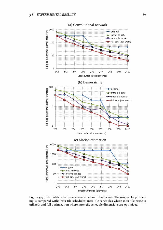
5.8. EXPERIMENTAL RESULTS 87
(a) Convolutional network
(b) Demosaicing
(c) Motion estimation
Figure 5.9: External data transfers versus accelerator buffer size. The original loop order-ing is compared with: intra-tile schedules; intra-tile schedules where inter-tile reuse is utilized; and full optimization where inter-tile schedule dimensions are optimized.
1
10
100
1000
2^2 2^3 2^4 2^5 2^6 2^7 2^8 2^9 2^10
x ti
mes
min
imu
m e
xte
rnal
tra
nsf
ers
Local buffer size [elements]
original
intra-tile opt.
inter-tile reuse
full-opt. (our work)
1
10
100
2^2 2^3 2^4 2^5 2^6 2^7 2^8 2^9 2^10
x ti
me
s m
inim
um
ext
ern
al t
ran
sfer
s
Local buffer size [elements]
original
intra-tile opt.
inter-tile reuse
full-opt. (our work)
1
10
100
1000
10000
2^2 2^3 2^4 2^5 2^6 2^7 2^8 2^9 2^10
x ti
mes
min
imu
m e
xte
rnal
tra
nsf
ers
Local buffer size [elements]
originalintra-tile opt.inter-tile reusefull-opt. (our work)

88 CHAPTER 5. INTER-TILE REUSE OPTIMIZATION
already reached with a buffer of 512 elements. A designer should stop increasing buffer size after this point, because the amount of data transfer stays constant and it only increases the area footprint.
5.8.2 Quality of results
As demonstrated, there is a trade-off between buffer size and communication requirements for hardware accelerators. In addition, the amount of compute re-sources influence the communication requirements. For HLS descriptions this is achieved by unrolling parts of algorithm code. As a result, the data path is replicated to utilize available parallelism, which requires more data to feed the extra compute resources. Figure 5.10 presents execution time measurements for different accelerator configurations. Accelerators with a small buffer (e.g. 32 el-ements like a register file) are bandwidth limited, so throughput will not scale with extra compute resources.
The quality of implemented accelerator schedules is evaluated by comparing execution time with resource usage. For FPGAs, resource usage is defined as: MAX(%DSPs, %BRAMs, %LUTs, %flip-flops). In Figure 5.11 the execution time versus resource usage is visualized by plotting the design points of figure Figure 5.10. In addition, the area-delay product is used to define the efficiency of differ-ent implementations. For each benchmark the best area-delay product is extrap-olated and plotted as a dotted line in the comparison.
The results for the ConvNet and Demosaicing application behave intuitive. Designs that are balanced score close to the dotted line, while designs severely limited by either compute or buffer resources occur further from this line. As predicted in Figure 5.9 for Demosaicing increasing the buffer size beyond 512 entries does not improve the design any further. However, for Motion Estima-tion a few results behave counter intuitive, e.g. increasing parallelism in small data buffer designs can reduce the resource usage. Vivado HLS is a production tool, and therefore a small change in the input description can trigger different optimizations. Due to unrolling with a factor two the number of required LUTs in the 32 and 64 entry designs are reduced, which reduces overall resource usage and the area delay product.
Finally, the best accelerators are compared with other platforms, as shown in Table 5.1. These accelerators do not have a dedicated DMA controller, which se-verely constraints the available communication bandwidth. However our inter-tile accelerators can increase the original MicroBlaze performance by 16 to 82 times, at the cost of a very small increase of overall resource usage. Hence simple embedded processors can perform on par with a high-end general purpose pro-cessor. Dedicated DMA can be added, but it will only shift the result of Figure 5.11.
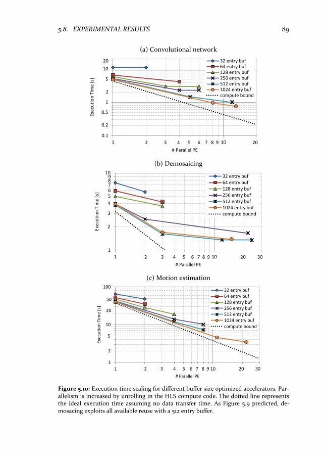
5.8. EXPERIMENTAL RESULTS 89
(a) Convolutional network
(b) Demosaicing
(c) Motion estimation
Figure 5.10: Execution time scaling for different buffer size optimized accelerators. Par-allelism is increased by unrolling in the HLS compute code. The dotted line represents the ideal execution time assuming no data transfer time. As Figure 5.9 predicted, de-mosacing exploits all available reuse with a 512 entry buffer.
0.1
1
10
1 10
Exe
cuti
on
Tim
e [s
]
# Parallel PE
32 entry buf64 entry buf128 entry buf256 entry buf512 entry buf1024 entry bufcompute bound
2 3 4 5 6 7 8 9 20
5
0.5
0.2
2
20
1
10
1 10
Exe
cuti
on
Tim
e [s
]
# Parallel PE
32 entry buf64 entry buf128 entry buf256 entry buf512 entry buf1024 entry bufcompute bound
2 3 4 5 6 7 8 9 20 30
98765
4
3
2
1
10
100
1 10
Exe
cuti
on
Tim
e [s
]
# Parallel PE
32 entry buf64 entry buf128 entry buf256 entry buf512 entry buf1024 entry bufcompute bound
2 3 4 5 6 7 8 9 20 30
5
50
20
2

90 CHAPTER 5. INTER-TILE REUSE OPTIMIZATION
(a) Convolutional network
(b) Demosaicing
(c) Motion estimation
Figure 5.11: FPGA resource utilization for accelerator mappings with an inter-tile itera-tion order. The best area delay product is selected as most efficient solution and extrap-olated by the dotted line.
0.1
1
10
0.1% 1.0%
Exe
cuti
on
Tim
e [s
]
FPGA Resources Used
32 entry buf64 entry buf128 entry buf256 entry buf512 entry buf1024 entry bufarea delay prod.
0.2% 0.5% 2.0% 5.0%
0.2
0.5
2
5
20
1
10
0.1% 1.0%
Exe
cuti
on
Tim
e [s
]
FPGA Resources Used
32 entry buf64 entry buf128 entry buf256 entry buf512 entry buf1024 entry bufarea delay prod.
98765
4
3
2
0.5% 5.0%0.2% 2.0%
1
10
100
0.1% 1.0%
Exe
cuti
on
Tim
e [s
]
FPGA Resources Used
32 entry buf64 entry buf128 entry buf265 entry buf512 entry buf1024 entry bufarea delay prod.
0.2% 0.5% 2.0%
2
5
20
50

5.8. EXPERIMENTAL RESULTS 91
Platform Demosaic [s] Block Match [s] ConvNet [s]
Intel-i7 0.54 8.12 0.63 Arm-A9 5.75 72.32 5.92 MicroBlaze 22.10 283.96 19.05 Accelerator 1.36 3.45 0.75
Table 5.1: Execution time comparison for multiple platforms.
5.8.3 Energy consumption
In the previous section throughput and resource utilization are evaluated. An-other key parameter for embedded systems is energy efficiency. Energy con-sumption is evaluated by FPGA bit toggling simulations for the real applications. To measure bit toggling during application runtime the Xilinx ISIM simulator is used. This simulator performs a behavioural simulation of the MicroBlaze core including connected peripherals like the Memory Interface Controller (MIC), or dedicated accelerators. Due to the excessive simulation time of such large sys-tems only 1 ms of the real workload (the initialization part is not recorded) is recorded in a Switching Activity Interchange Format (SAIF) file.
The Xilinx XPower tools combine the SAIF file with the placed and routed design to estimate the FPGA power usage. For a complete power figure we in-cluded the activity of the external DDR3 memory module. This is performed by recording the output of the Xilinx soft-core memory controller, and feed the memory command sequence to a DDR3 memory energy estimator [17].
The estimated system power consumption during 1 ms of effective workload is extrapolated to the run time of each complete application. Figure 5.12 presents the energy consumption to run each complete application for the different map-pings. These figures demonstrate that even the very small accelerators with 32 buffer entries can substantially improve energy efficiency, factors of 2.5 up to 5.8 better efficiency are shown. However, if data transfer is reduced aggressively by using the best area delay product mappings energy efficiency increases by 18 to 82 times compared to the MicroBlaze mapping.
The huge energy efficiency improvement is mainly caused by execution time reduction, since dynamic power usage changes only by a small amount. The ex-act power figures are outlined in Table 5.2, which reveals that the major portion of power consumption is static. This is mainly due to large design area used for the Memory Interface Controller and the MicroBlaze core, see Figure 5.13. These results indicate that the addition of the relatively small accelerators does not increase power usage significantly. In addition, though the use of efficient data reuse in local buffers the data movement does not increase. The relatively small accelerators and optimized data reuse schedules do not increase power usage, but they reduce execution time tremendously which gives a boost to energy ef-ficiency. Although energy efficiency improved a lot, the energy per effective op-eration is still 1 to 7 nJ depending on the application data reuse. For smartphone or wearable scenarios this is a good step forward, but not enough. These use cases require one or two orders of magnitude efficiency improvement.
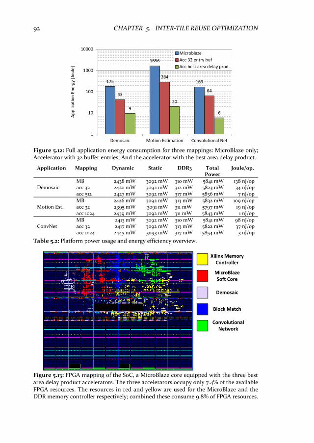
92 CHAPTER 5. INTER-TILE REUSE OPTIMIZATION
Figure 5.12: Full application energy consumption for three mappings: MicroBlaze only; Accelerator with 32 buffer entries; And the accelerator with the best area delay product.
Application Mapping Dynamic Static DDR3 Total Power
Joule/op.
Demosaic MB 2438 mW 3092 mW 310 mW 5841 mW 138 nJ/op acc 32 2420 mW 3092 mW 312 mW 5823 mW 34 nJ/op acc 512 2427 mW 3092 mW 317 mW 5836 mW 7 nJ/op
Motion Est. MB 2426 mW 3092 mW 313 mW 5832 mW 109 nJ/op acc 32 2395 mW 3091 mW 311 mW 5797 mW 19 nJ/op acc 1024 2439 mW 3092 mW 311 mW 5843 mW 1 nJ/op
ConvNet MB 2413 mW 3092 mW 310 mW 5841 mW 98 nJ/op acc 32 2417 mW 3092 mW 313 mW 5822 mW 37 nJ/op acc 1024 2445 mW 3093 mW 317 mW 5854 mW 3 nJ/op
Table 5.2: Platform power usage and energy efficiency overview.
Figure 5.13: FPGA mapping of the SoC, a MicroBlaze core equipped with the three best area delay product accelerators. The three accelerators occupy only 7.4% of the available FPGA resources. The resources in red and yellow are used for the MicroBlaze and the DDR memory controller respectively; combined these consume 9.8% of FPGA resources.
175
1656
169
43
284
64
9
20
6
1
10
100
1000
10000
Demosaic Motion Estimation Convolutional Net
Ap
plic
atio
n E
ner
gy [
Jou
le]
Microblaze
Acc 32 entry buf
Acc best area delay prod.
Xilinx Memory Controller
MicroBlaze Soft Core
Demosaic
Block Match
Convolutional Network

5.9. CONCLUSIONS 93
5.9 Conclusions
In this Chapter we presented our new inter-tile reuse optimization strategy for nested loop accelerators. This optimization strategy searches the best combina-tion of loop interchange and tiling with optimal tile sizes. We demonstrated that maximizing efficiency for local buffers in FPGA based accelerators gives a sub-stantial performance improvement. These improvements are enabled by effi-ciently exploiting local buffering with data access optimizations for nested loops. Our optimizations manage to limit buffering requirements while achieving a sig-nificant reduction of external data transfer. The main improvement is achieved by optimizing for inter-tile reuse. Although the design space can be huge and chaotic for deeply nested loops, we show that the best configuration of transfor-mations can be found with a model-based approach. Our focus on inter-tile re-use effectively prunes the search space of configurations, and limits the effort of exploration to mere seconds. The fruits of our optimizations are verified with the Xilinx Vivado HLS tools, and we observe a significant reduction in the effort of designing efficient dedicated accelerators. With our approach the number of required design iterations is minimized, by directly computing the best candi-dates before time consuming synthesis. As a result, the mapping process of static image or video processing applications to dedicated hardware accelerators is much better manageable.
94
6.
NVE: A FLEXIBLE ACCELERATOR
As outlined in the earlier chapters Convolutional Networks (ConvNets) en-able record breaking classification performance for many daily tasks. How-ever the associated demands on computation and data transfer prohibit straightforward adoption by energy constrained wearable consumer plat-forms. The computational burden can be overcome by dedicated hardware accelerators, but it is the sheer amount of data transfer, and level of utili-zation that largely determines the energy-efficiency of such implementa-tions. This chapter presents the Neuro Vector Engine (NVE) a SIMD accelerator template for ConvNet based vision applications, targeting the consumer market, in particular the ultra-low power wearable devices. The NVE is very flexible due to the use of a VLIW ISA, which comes at the cost of instruction fetch overhead. We demonstrate that this overhead is insig-nificant when the flexibility enables advanced data locality optimizations from the previous chapters. In addition, our flexibility ensures an excellent hardware utilization for different ConvNet vision applications. By co-opti-mizing accelerator architecture and applying the inter-tile reuse optimiza-tion methodology, 30 Gops is achieved within a power envelope of 54 mW and only 0.26 mm2 silicon footprint in TSMC 40 nm technology. These per-formance numbers enable high-end visual object recognition by portable and even wearable devices. This chapter is based on work presented at DATE 2016 [109].
6.1 Introduction
Although Convolutional Networks (ConvNets) achieve superior results for ma-chine vision, they lack an attribute crucial for mobile and wearable applications, and that is energy-efficiency. The rather large computational workload and data intensity has motivated optimized implementations on CPUs [18], GPUs [28] and FPGAs [108,155]. All these implementations do not fit the very constrained (less
CHAPTER

6.1. INTRODUCTION 95
than 1 Watt) mobile power budget. In Chapter 5 we demonstrated with dedi-cated FPGA accelerators that it is very challenging to reach the sub 1 Watt target while achieving sufficient compute performance. Although FPGAs have the flex-ibility to reprogram the data path their operators simply consume too much en-ergy compared to their ASIC counterparts. On the other hand, instruction based CPUs or GPUs spend way too much energy on non-compute related control structures, e.g. instruction fetch, decode, pipeline management, program se-quencing, etc.
The computer architecture community is well aware of the trend towards heterogeneous computing where architecture specialization is used to achieve high performance at low energy [58]. A few research groups use the customiza-tion paradigm to design highly specialized hardware accelerators that could en-able excellent machine vision for mobile devices [16,50,20]. The main challenge in accelerator design is to reconcile architecture specialization and flexibility. Especially, the right level of flexibility is key for the energy-efficiency of an ac-celerator. ConvNets have many parameters such as the layers, feature maps, and kernels, which are different for every task. Hence the architecture should sup-port different parameters efficiently, and on the other hand data storage struc-tures should be tuned to the data-flow and data-locality requirements. Earlier works focused on this last aspect by focusing on efficiently implementing the compute primitives. However, by adding more flexibility we demonstrate an ad-ditional efficiency improvement that is counter intuitive, but crucial for real-world ConvNet vision applications.
In this chapter we present the Neuro Vector Engine (NVE), an ultra-efficient accelerator template for ConvNet based vision applications. The design builds on efficient SIMD operations that focus on data reuse opportunities by employ-ing a local scratchpad buffer. The VLIW ISA enables a very high utilization; real-world benchmarks demonstrate an excellent silicon area efficiency (perfor-mance/area = 115 Gops/mm2). In addition, the VLIW ISA enables advanced data locality optimizations that increase energy efficiency tremendously (perfor-mance/power = 559 Gops/W). Our main contributions are:
• A new ultra-low power accelerator template for ConvNets.
• The first extremely flexible ConvNet accelerator with full VLIW com-piler support.
• Extensive evaluation of the architectural design involving data move-ment analysis due to the inter-tile data locality optimization.
• Detailed comparison with a low-power ARM-A9 core and an embedded NVIDIA TK1 GPU.
First, Section 6.2 gives an overview of related work. Next in Section 6.3 the inefficiencies of general purpose CPUs are analyzed. In Section 6.4 these ineffi-ciencies are addressed by the NVE architecture. Section 6.5 presents an in depth evaluation of the NVE architecture. Section 6.6 will evaluate different instances of the template and will discuss limitations and future work. The chapter is fi-nalized with conclusions in Section 6.7.

96 CHAPTER 6. NVE: A FLEXIBLE ACCELERATOR
6.2 Related work
The energy constraints on mobile and embedded devices, forces researchers to find solutions that improve efficiency. In this search others have proposed cus-tom accelerator architectures of ConvNets for FPGA or ASIC. In this section we will investigate popular architectures that are proposed in the literature. We will show that most of the work is too specific, i.e. when different networks must be supported the efficiency drops substantially.
Many works focus on a computational operator that implements the filtering part in a ConvNet. Filtering represents 90% of the computational workload, so it is an important part. A systolic implementation seems a natural fit since these structures are very efficient at filtering. Two popular works propose the use of a systolic implementation of a 2D convolution operation [16,50]. Figure 6.1 illus-trates the architectural concept of a systolic array for 2D convolution. In this structure the weight coefficient registers w11-wkk are programmed by a host pro-cessor. Next, image lines are streamed in and the outputs are streamed out for a complete output image. No instructions are required only input and output streams and almost all resources are dedicated to the computation.
Although systolic implementations are computationally efficient they have limited flexibility. For example, running the benchmark networks from Chap-
Image row m+1
Image row m
Image row m+K
*
W1K
+
*
W1K-1
+
*
W11
+
*
W2K
+
*
W2K-1
+
*
W21
+
*
WKK
+
*
WKK-1
+
*
WK1
+
+
+
+
OUT
Load from off-chip DRAM
KFIFOsline memories
K2+K DSP units chained
B1
Figure 6.1: Architecture of a systolic 2d convolution operation [119]. The systolic struc-ture has a peak throughput of one KxK dot product per cycle. For K=7 this results in 49 MACC operations per cycle. For a single 2d convolution all data reuse is exploited.
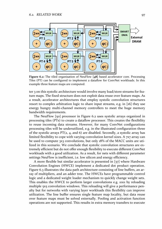
6.2. RELATED WORK 97
ter 3 on this systolic architecture would involve many load/store streams for fea-ture maps. The fixed structure does not exploit data reuse over feature maps. As a result, accelerator architectures that employ systolic convolution structures resort to complex arbitration logic to share input streams, e.g. in [16] they use energy hungry multi-channel memory controllers to meet the huge memory bandwidth requirements.
The NeuFlow [50] processor in Figure 6.2 uses systolic arrays organized in processing tiles (PTs) to create a dataflow processor. This creates the flexibility to reuse incoming data streams. However, for many ConvNet configurations processing tiles will be underutilized, e.g. in the illustrated configuration three of the systolic arrays PT(2, 4, and 6) are disabled. Secondly, a systolic array has limited flexibility to cope with varying convolution kernel sizes. A 7x7 array can be used to compute 3x3 convolutions, but only 18% of the MACC units are uti-lized in this scenario. We conclude that systolic convolution structures are ex-tremely efficient but do not offer enough flexibility to execute different ConvNet workloads with a good utilization. As a result, for nets with different parameter settings NeuFlow is inefficient, i.e. low silicon and energy efficiency.
A more flexible but similar accelerator is presented in [37] where Hardware Convolution Engines (HWCE) implement a dedicated dot product operation. Figure 6.3 illustrates the data path architecture consisting of line buffers, an ar-ray of multipliers, and an adder tree. The HWCEs have programmable control logic and a dedicated weight loader mechanism to quickly change weight sets. This enables the HWCE to perform larger convolutions e.g. 11x11 by reloading multiple 5x5 convolution windows. This reloading will give a performance pen-alty but for networks with varying layer workloads this flexibility can improve utilization. The line buffer ensures single feature map locality, but data reuse over feature maps must be solved externally. Pooling and activation function operations are not supported. This results in extra memory transfers to execute
Figure 6.2: The tiled organisation of NeuFlow [48] based accelerator core. Processing Tiles (PT) can be configured to implement a dataflow for ConvNet workloads. In this example three feature maps are computed.
PT 1
MUX
+ φ( )
PT 2
MUX
+ φ( )
PT 3
MUX
+ φ( )
PT 4
MUX∑wx
+ φ( )
PT 5
MUX
+ φ( )
MUX
+ φ( )
∑wx∑wx
∑wx∑wx
∑wx
PT 6
SMART
DMAExternal DRAM

98 CHAPTER 6. NVE: A FLEXIBLE ACCELERATOR
these steps in software. The HWCEs are integrated in a multi-core RISC cluster, so moving the missing parts to software is possible but it reduces energy effi-ciency.
Another important work is DianNao [20], a high-throughput standalone pipelined accelerator core. Similar to the other accelerators DianNao imple-ments a dot product operator, see the pipelined datapath in Figure 6.4. The im-plemented dot product operator is more configurable compared to other works. The first stage is a multiplier stage, followed by a reduction stage that configures adder trees or implements max pooling operators. The last stage performs acti-vation function interpolation. Multiple multipliers are used to exploit the paral-lelism over many input feature maps. The rationale is that convolution windows have 5x5 sizes where the number of input maps in large networks can run into hundreds. Utilizing parallelism only over input feature maps and not over win-dow operations makes that the input vector is 1d instead of 2d. By repeating the 1d operation for multiple input window positions a convolution window is con-structed.
Compared to earlier works DianNao focusses much more on data locality in the reuse buffers. They use separate buffers for synaptic weights (SB), input maps (NBin) and output maps (NBout). These buffers hold vectors with the data ele-ments. The vectors do not exploit reuse over different convolution kernel posi-tons, so unique weights are send out into the data path causing many loads from the SB memory. DianNao focusses on very large networks with many feature maps. However, the face detection workload from Chapter 3 reveals that vision applications can have ConvNets with only few input feature maps per layer. This severely limits the parallelism that can be used by the DianNao accelerator re-sulting in underutilization.
All these architectures implement a dedicated dot product operator, some in a streaming pipeline others as a configurable operator. For all these accelerators we observe significant flexibility issues. If the network operators are tuned to the
Line Buffer
*0 *24 *0 *24
W 25 px (16bit)
Xin
ADDER TREE
ADDER TREE
Yin
1 packet(32bit)
1 packet(32bit)
25 px (16bit)
25 px (16bit)25 px (16bit)
1 px (16bit)1 px (16bit) 1 packet
(32bit)
Figure 6.3: Hardware Convolution Engine (HWCE) unit, used as accelerator for Con-vNets in [36].

6.3. SOURCES OF INEFFICIENCY IN GENERAL PURPOSE CPUS 99
accelerator data path a good efficiency level can be achieved. However a Con-vNet with different parameters results in a substantial reduction of efficiency. The goal of the Neuro Vector Engine is to deliver a constant and high efficiency level on different ConvNets. To achieve a more constant and high efficiency level more control flexibility is necessary. This is a challenging goal, because often this control flexibility results in a reduced efficiency.
6.3 Sources of inefficiency in general purpose CPUs
In the previous section we showed the utilization problem for very dedicated accelerator cores. When multiple networks with varying parameters are used the efficiency often drops substantially. To increase accelerator flexibility we study the properties of general purpose CPUs but we try to minimize their excessive inefficiency’s.
It is well known in the domain of computer architecture that general-purpose processors spend most energy on instruction control. This definitely holds for advanced out-of-order superscalar designs that consume a lot of energy in the instruction reorder part. The energy consumption of a much simpler RISC pro-cessors is also dominated by instruction overheads such as instruction fetch, de-code, pipeline management, program sequencing, etc. This energy consumption distribution is extensively studied in [113,58]. Figure 6.5 illustrates the energy distribution for a simple RISC (45 nm @ 0.9V technology) ADD instruction, which consumes about 70 pJ of energy. A load/store type of instruction would use the data cache and increases instruction energy to 95 pJ. The energy dissipa-
+*
*
*
*
+
+
+
+
+
φ
φ
NFU-1 NFU-2 NFU-3
NBin
SB
NBout
Me
mo
ry Inte
rface
Control Processor (CP)
Figure 6.4: The pipelined data path of the DianNao accelerator core [19]. Separate mem-ories load vectors for

100 CHAPTER 6. NVE: A FLEXIBLE ACCELERATOR
tion in a functional unit to add two 32-bit numbers is only 0.5 pJ. This huge dif-ference in energy consumption demonstrates that the useful fraction of energy
in an ADD operation is only 1
140. In practice it is even worse, because such oper-
ations are often done in loops that require overhead instructions for loads and branching. Overhead instructions further reduce the useful energy fraction to 1
850. This example clarifies why custom accelerators can be 100 times more effi-
cient than general purpose CPUs, they simply don’t need all those instructions. To use the flexibility of instruction programmed accelerators, but with a
much better energy efficiency the overhead should be drastically reduced. 1. Many useful operations should be performed per instruction. This can be
achieved by the Single Instruction Multiple Data (SIMD) paradigm. E.g., a 16 element vector ADD could increase the amount of useful work per in-
struction from 1
140 to
1
10, see Figure 6.6.
2. The ratio of useful instructions should be high, so overhead instructions should be minimized. This involves minimizing the number of load/store operations (locality), and replacing them by more efficient vector load/stores. An instruction pattern as depicted in Figure 6.6 improves the
loop efficiency from 1
850 to
1
18. Note that control instructions like the branch
are replaced by a hardware loop counter. Switching to vector instructions and increasing register level data reuse im-proves the energy efficiency almost by 50 times. This does not result in the same efficiency levels as presented by dedicated accelerators, but it will give a much higher degree of flexibility. In addition, other optimizations like loop transfor-mations, fixed point precision exploration, should be applied to further increase the efficiency. Motivated by this example of processor architecture modifica-tions towards a flexible and efficient accelerator we developed the Neuro Vector Engine (NVE). An accelerator template based upon energy efficient processors. The NVE is positioned between the design points of high efficiency custom ac-celerators and general purpose processors. This to combine the best of both worlds, high efficiency, good utilization and a high degree of flexibility.
LD
LD
ADD
ST
BR
D-cache access
I-cache access
Register access
Control ALU
25 pJ
25 pJ
25 pJ
25 pJ
25 pJ
25 pJ
25 pJ
25 pJ
4 pJ
4 pJ
4 pJ
4 pJ
4 pJ
32-bit ADD ≈ 0.5 pJ
Overhead instructions
Overhead instructions
Figure 6.5: Instruction energy breakdown for a typical addition loop executed by a 45 nm RISC core at 0.9V [54,107]. Note the very small portion of energy spend on the actual addition. This is an example of the large inefficiencies in general purpose CPUs.

6.4. THE NEURO VECTOR ENGINE (NVE) ARCHITECTURE 101
6.4 The Neuro Vector Engine (NVE) architecture
In this section our flexible NVE accelerator template is outlined. As the name suggests all operations are done on vectors to achieve a good efficiency. A bal-ance between efficiency and flexibility is created with a VLIW based processor template that is equipped with vector operations tuned for ConvNets. Figure 6.7 illustrates the 6 issue slot VLIW template. A VLIW organization gives flexibility to program the accelerator for different ConvNet workloads. Secondly this tem-plate supports the advanced access patterns required for inter-tile data reuse optimization, see Chapter 5. Here we focus on a single instance of the template, but custom modifications can be easily performed. We will comment on possible modifications at the end of this section.
6.4.1 Vector data path
Often systolic or dedicated convolution operators are used in custom accelera-tors (see Section 6.2). The NVE uses a different and more flexible iterative oper-ation for the computation of convolutions. The main compute operation is a vector Multiply Accumulate (MACC), i.e. �⃗� ← �⃗� + �⃗� × 𝑤. It modifies an array of accumulator values �⃗� where each value represents a neighbouring neuron. By sequentially repeating this operation over all inputs of a 2D or 3D convolution window the reduction operation is performed. For varying kernel sizes a MACC resource is well utilized. Other accelerators use dedicated adder trees for the reduction [20,37] which has the disadvantage that reconfiguring for other kernel sizes is costly. The usage of accumulation registers in the NVE makes it relatively simple to implement other operations like the MAX operation used in max pool-ing layers.
SIMD OP 25 pJ 8 pJ
25 pJ 8 pJSIMD OP
SIMD OP 25 pJ 8 pJ
25 pJ 8 pJSIMD OP
50 pJ 8 pJ25 pJ
50 pJ 8 pJ25 pJ
SIMD LD
SIMD ST
D-cache access I-cacheVect.
Register Control 16 lane SIMD ALU
Figure 6.6: Instruction energy breakdown for a simple SIMD processor. Vector loads and register accesses consume more energy than scalar ones. However, reduction of overhead instructions and a substantial increase of useful work improves efficiency by 50 times compared to the scalar version.
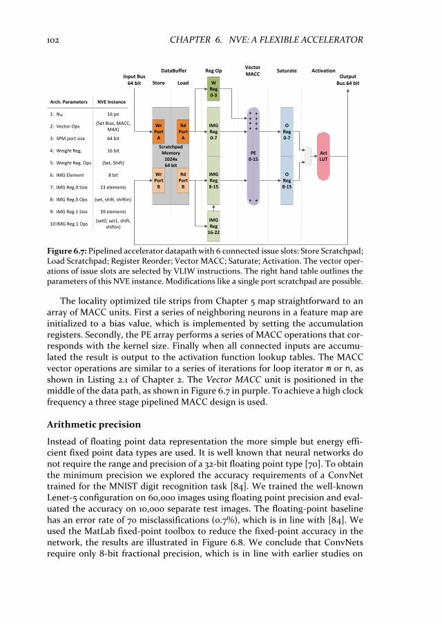
102 CHAPTER 6. NVE: A FLEXIBLE ACCELERATOR
The locality optimized tile strips from Chapter 5 map straightforward to an array of MACC units. First a series of neighboring neurons in a feature map are initialized to a bias value, which is implemented by setting the accumulation registers. Secondly, the PE array performs a series of MACC operations that cor-responds with the kernel size. Finally when all connected inputs are accumu-lated the result is output to the activation function lookup tables. The MACC vector operations are similar to a series of iterations for loop iterator m or n, as shown in Listing 2.1 of Chapter 2. The Vector MACC unit is positioned in the middle of the data path, as shown in Figure 6.7 in purple. To achieve a high clock frequency a three stage pipelined MACC design is used.
Arithmetic precision
Instead of floating point data representation the more simple but energy effi-cient fixed point data types are used. It is well known that neural networks do not require the range and precision of a 32-bit floating point type [70]. To obtain the minimum precision we explored the accuracy requirements of a ConvNet trained for the MNIST digit recognition task [84]. We trained the well-known Lenet-5 configuration on 60,000 images using floating point precision and eval-uated the accuracy on 10,000 separate test images. The floating-point baseline has an error rate of 70 misclassifications (0.7%), which is in line with [84]. We used the MatLab fixed-point toolbox to reduce the fixed-point accuracy in the network, the results are illustrated in Figure 6.8. We conclude that ConvNets require only 8-bit fractional precision, which is in line with earlier studies on
VectorMACC
IMGReg0-7
IMGReg8-15
IMG Reg
16-22
W Reg0-3
Reg Op
ScratchpadMemory
1024x64 bit
RdPort
A
RdPort
B
WrPort
A
LoadStore
OReg0-7
OReg8-15
Saturate ActivationDataBuffer
PE 0-15
+*+*+*+*
+*
Act LUT
WrPort
B
Input Bus 64 bit
Output Bus 64 bit
Arch. Parameters NVE Instance
1: NPE 16 pe
2: Vector Ops{Set Bias, MACC,
MAX}
7: IMG Reg.0 Size
8: IMG Reg.0 Ops
23 elements
{set, shift, shiftin}
3: SPM port size
5: Weight Reg. Ops {Set, Shift}
64 bit
4: Weight Reg. 16 bit
6: IMG Element 8 bit
9: IMG Reg.1 Size
10:IMG Reg.1 Ops
39 elements
{set0, set1, shift, shiftin}
Figure 6.7: Pipelined accelerator datapath with 6 connected issue slots: Store Scratchpad; Load Scratchpad; Register Reorder; Vector MACC; Saturate; Activation. The vector oper-ations of issue slots are selected by VLIW instructions. The right hand table outlines the parameters of this NVE instance. Modifications like a single port scratchpad are possible.

6.4. THE NEURO VECTOR ENGINE (NVE) ARCHITECTURE 103
classical neural nets. Table I, gives the exact configuration of the data types that are used in the NVE accelerator design. The MACC PE array has a 16-bit (weight) and 8-bit (neuron) input that are used by a truncated multiplication. The accu-mulation register is extended to 9 integer bits with a hardware check to prevent overflow. Before activation function lookup the accumulation value is saturated to the 10-bit potential format given in Table 6.1. The Activation Function is im-plemented at the end of the pipeline with a look-up memory of 1024 entries of 8-bit, see Figure 6.7. As a result it is possible to implement any activation func-tion efficiently by reloading the activation LUT.
6.4.2 Memory system
To exploit the inter-tile reuse opportunities that are proposed in Chapter 5 a programmable and flexible memory system is implemented. There is no need for expensive caches, because the access functions in ConvNets are static and pred-icable. Hence, we use an efficient scratch pad memory and vector reorder regis-ters to exploit data reuse. Separating the accessing of values over two different data structures gives a huge complexity reduction. A 2D register file or scratch pad with reordering functionalities would be complex. Therefore 1D reordering is performed in L0 (registers), and the orthogonal 1D reordering by reloading in L1 (scratchpad).
L0: Vector reorder registers
To feed the vector MACC unit with weight coefficients and input values dedi-cated vector reorder registers are used. These registers are located in the Reg Op
Table 6.1: Fixed-point data word configurations for the NVE instantiation.
Data type Word size Fixed point format
Weights 16 bit SIIIIIII.FFFFFFFF
In/Act 8 bit .FFFFFFFF
Potential 10 bit SIII.FFFFFF
Figure 6.8: ConvNet fixed point accuracy exploration for varying fractional precision.
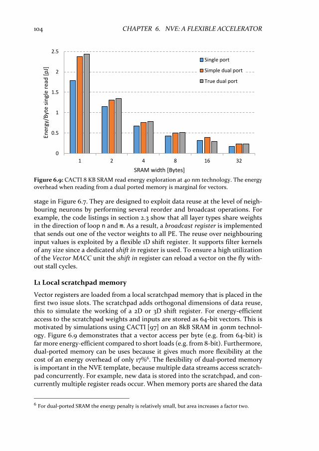
104 CHAPTER 6. NVE: A FLEXIBLE ACCELERATOR
stage in Figure 6.7. They are designed to exploit data reuse at the level of neigh-bouring neurons by performing several reorder and broadcast operations. For example, the code listings in section 2.3 show that all layer types share weights in the direction of loop n and m. As a result, a broadcast register is implemented that sends out one of the vector weights to all PE. The reuse over neighbouring input values is exploited by a flexible 1D shift register. It supports filter kernels of any size since a dedicated shift in register is used. To ensure a high utilization of the Vector MACC unit the shift in register can reload a vector on the fly with-out stall cycles.
L1 Local scratchpad memory
Vector registers are loaded from a local scratchpad memory that is placed in the first two issue slots. The scratchpad adds orthogonal dimensions of data reuse, this to simulate the working of a 2D or 3D shift register. For energy-efficient access to the scratchpad weights and inputs are stored as 64-bit vectors. This is motivated by simulations using CACTI [97] on an 8kB SRAM in 40nm technol-ogy. Figure 6.9 demonstrates that a vector access per byte (e.g. from 64-bit) is far more energy-efficient compared to short loads (e.g. from 8-bit). Furthermore, dual-ported memory can be uses because it gives much more flexibility at the cost of an energy overhead of only 17%6. The flexibility of dual-ported memory is important in the NVE template, because multiple data streams access scratch-pad concurrently. For example, new data is stored into the scratchpad, and con-currently multiple register reads occur. When memory ports are shared the data
6 For dual-ported SRAM the energy penalty is relatively small, but area increases a factor two.
0
0.5
1
1.5
2
2.5
1 2 4 8 16 32
Ener
gy/B
yte
sin
gle
read
[p
J]
SRAM width [Bytes]
Single port
Simple dual port
True dual port
Figure 6.9: CACTI 8 KB SRAM read energy exploration at 40 nm technology. The energy overhead when reading from a dual ported memory is marginal for vectors.

6.4. THE NEURO VECTOR ENGINE (NVE) ARCHITECTURE 105
path should stall more often, which reduces hardware utilization. One could use multiple separate memories e.g., for weights, inputs, and temporal results. How-ever it is very difficult to effectively utilize the capacity and throughput of these memories. Each layer has different requirement w.r.t. the ratio of weights and inputs, so with a single shared flexible buffer we can utilize buffer capacity and throughput over different workloads.
6.4.3 Control and programming
The NVE architecture exist of 6 successive issue slots; each performs a different functionality. The control of issue slots is distributed over one Very Long In-struction Word (VLIW). Using instructions improves flexibility substantially at the cost of instruction fetch overhead. Each issue slot is very specific so the in-struction width can be small (54-bit). To minimize the overhead we use three techniques:
1. An energy-efficient on-chip loop buffer that holds 512 instructions. 2. Modulo software pipelining [80] to efficiently fold instructions together. 3. Modulo address generators to remove many instructions.
In addition, all issue slot operations of the NVE are performed on vectors, which increases the amount of useful work per instruction, see Section 6.3.
Software pipelining
A high data path utilization with a small code size is achieved by software pipe-lining operations of successive issue slots. The basic idea is to translate the re-petitive operations in a tile strip to a steady-state description. Many iterations of the steady-state are repeated to execute a complete tile strip, which improves instruction reuse. As an educational example the steady-state program of 16 con-current rows of 3x3 convolution is given in Figure 6.10. Note that our techniques push a lot of work from each instruction. Each steady-state (10 instructions) pro-cess 16 dot products (144 MACC operations) this excludes, load/stores, vector
st [s(i+2) word0]
ld [s(i+2) word0]
MEM B
ld [s(i+0) word1] shift
WREG
set [b w0 w1 -]
shift
macc rw,ri
VMACC
set rw
macc rw,ri
macc rw,ri
macc rw,ri
shift
set [w5 w6 w7 w8]
set [w2 w3 w4 -]
ld [s(i+1) word1]
ld [s(i+0) word2]
shift
shift
macc rw,ri
macc rw,ri
macc rw,ri
shift
ld [s(i+2) word1]
MEM A WB Sgm
act [s(i-1) word0]
act [s(i-1) word1]
ld [s(i+2) word2]
shift
ld [s(i+1) word2]
1
2
3
4
5
6
7
8
9
10
Cycle
ld [b w0 w1 -]
ld [s(i+0) word0]
st [s(i+2) word1]
ld [w2 w3 w4 -]
ld [s(i+1) word0]
st [s(i+2) word2]
ld [w5 w6 w7 w8]
shift
IREG
set r0,r1
set r2 shift
shift
shift
set r2 shift
set r0,r1
set r2 shift
set r0,r1
macc rw,ri
macc rw,ri
Figure 6.10: VLIW assembly description of a steady-state program for 3x3 convolution in a feature map. Note that control is distributed over the different NVE issue-slots. Image load/stores of the scratchpad use modulo addressing over steady-state iterations to max-imize the storage efficiency (i.e. old data is immediately overwritten by new).
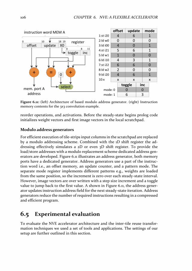
106 CHAPTER 6. NVE: A FLEXIBLE ACCELERATOR
reorder operations, and activations. Before the steady-state begins prolog code initializes weight vectors and first image vectors in the local scratchpad.
Modulo address generators
For efficient execution of tile-strips input columns in the scratchpad are replaced by a modulo addressing scheme. Combined with the 1D shift register the ad-dressing effectively simulates a 2D or even 3D shift register. To provide the load/store addresses with a modulo replacement scheme dedicated address gen-erators are developed. Figure 6.11 illustrates an address generator, both memory ports have a dedicated generator. Address generators use a part of the instruc-tion word i.e., an offset memory, an update counter, and a pattern mode. The separate mode register implements different patterns e.g., weights are loaded from the same position, so the increment is zero over each steady-state interval. However, image vectors are over written with a step size increment and a toggle value to jump back to the first value. A shown in Figure 6.11, the address gener-ator updates instruction address field for the next steady-state iteration. Address generators reduce the number of required instructions resulting in a compressed and efficient program.
6.5 Experimental evaluation
To evaluate the NVE accelerator architecture and the inter-tile reuse transfor-mation techniques we used a set of tools and applications. The settings of our setup are further outlined in this section.
Figure 6.11: (left) Architecture of based modulo address generator. (right) Instruction memory contents for the 3x3 convolution example.
updateoffset
= +
selectmem. port A address
0+
toggle inc
X00 1810 19
0 8 11
modeupdateoffset164000104165
1:st i20
2:ld w0
3:ld i00
4:st i21
0015:ld w1
1346:ld i10
0667:st i22
0028:ld w2
9:ld i20 16410:x xxx
inctoggle0036
mode: 0
mode: 1
register
instruction word MEM A

6.5. EXPERIMENTAL EVALUATION 107
6.5.1 Benchmark setup
To NVE architecture is evaluated with the two Convolutional Network recogni-tion applications introduced in Chapter 3. These applications are the Face de-tection network [53], and Speed sign detection [105]. In addition, the educational example of 3x3 convolution is used for evaluation. All applications run on a HD720p video stream and for best performance we use the optimized imple-mentations with merged convolution and subsample layers as described in Chapter 4. The two real-world applications contain a mix of different layers with varying kernel sizes, dense and sparse connectivity, as detailed in Table 6.2.
Baseline commercial platform mappings
As baseline to compare the NVE an ARM Cortex-A9 core is selected. Due to its good energy efficiency and performance it is a popular embedded platform in many Smartphones. In addition, we compare with an Nvidia Embedded GPU the Jetson TK1 with 192 Cuda cores [100]. The NVE is positioned as flexible IP core for the next generation of smart compute platforms, so the ARM A9 and Nvidia TK1 are direct competitors.
For fair comparison it is important that both ConvNet vision applications are optimized. For the ARM-A9, we used all compiler optimizations of GCC 4.7, which made the C implementation of speed sign detection 13.4x faster with an energy efficiency increase of 13.3x. In addition, usage of SIMD NEON intrinsics resulted in an extra speedup of 2.7x with an energy efficiency increase of 1.8x.
For the TK1 mapping we used a CUDA optimized mapping, e.g., we use the constant memory for coefficients, exploit tiling and memory access coalescing. For the ARM core we use a GEM5 [7] and McPAT [88] simulator setup. The model assumes a 4-issue superscalar core with 800MHz clock, 32kB instruction and 64kB data cache with an associativity of 2, and a line size of 64 bytes. McPAT is configured for low power operating mode in 40nm technology. The Jetson TK1 measurements are done on the NVidia development board.
Face Detection [53] No Ni Nm Nn Nk Nl S Layer 1 4 1 638 358 6 6 2 Layer 2 14 2 317 177 4 4 2 Layer 3 14 1 312 172 6 6 1 Layer 4 1 14 312 172 1 1 1
Speed Sign [105] No Ni Nm Nn Nk Nl S Layer 1 6 1 638 358 6 6 2 Layer 2 16 3 317 177 6 6 2 Layer 3 80 40 313 173 5 5 1 Layer 4 8 80 312 172 1 1 1
Table 6.2: Convolutional Network application parameters.

108 CHAPTER 6. NVE: A FLEXIBLE ACCELERATOR
NVE instantiation
For evaluation of the NVE architecture a 16 MACC PE data path with all control is designed in VHDL. The required memories in the design are configured as follows:
• 8 kB dual-port scratchpad with 64-bit entries
• 8 activation function LUT memories of 1 kB each
• a 54-bit wide 512 entry instruction buffer Although we target ASIC technology the functional correctness of the design is verified by FPGA mapping. For estimation of ASIC properties the design is syn-thesized with Cadence Encounter RTL Compiler from a 40 nm TSMC low power library. The SRAM memories are simulated with CACTI [97] for a similar 40nm low power library. The target clock frequency of 1 GHz is achieved by pipelining of the stages in the data path. It is important to enable retiming, since it reduced area by 32% and power consumption by 41%.
For accelerator mapping an optimizing compiler [107] is used. This compiler reads a JSON ConvNet descriptions that is automatically converted into opti-mized software pipelined VLIW programs. These programs are automatically converted into VHDL test benches that are simulated on the post-synthesis re-sult for energy estimation. An extensive review of this compiler is given in Chap-ter 7.
6.5.2 Accelerator characteristics
The total area footprint of the accelerator is 0.26 mm2, which makes it a very small design, e.g., the McPAT ARM core requires 14 mm2. The area breakdown of the different components in the synthesized accelerator is given in Table 6.3. From the results is observed that (71%) of the area is spend on the on-chip SRAM. Given the fact that the complete architecture aims at minimizing external com-munication by reusing data or instructions in local buffers this is in line with our expectation.
The power results are obtained by post-synthesis simulation of tile strips from the vision applications implemented as steady-state programs similar to the 3x3 convolution code in Figure 6.10. Table 6.3 presents the average power breakdown of the simulations. The major energy portion is consumed by the
Module Area [mm2] (%) Power [mW] (%) Accelerator 0.259 54.1
Logic 0.076 (29%) 43.3 (80%) Scratchpad 0.112 (43%) 5.9 (11%) Act. LUT 0.045 (17%) 1.5 (3%) Instr. Buf. 0.026 (10%) 3.4 (6%)
Table 6.3: Breakdown of synthesized area and power during simulation at 40 nm.
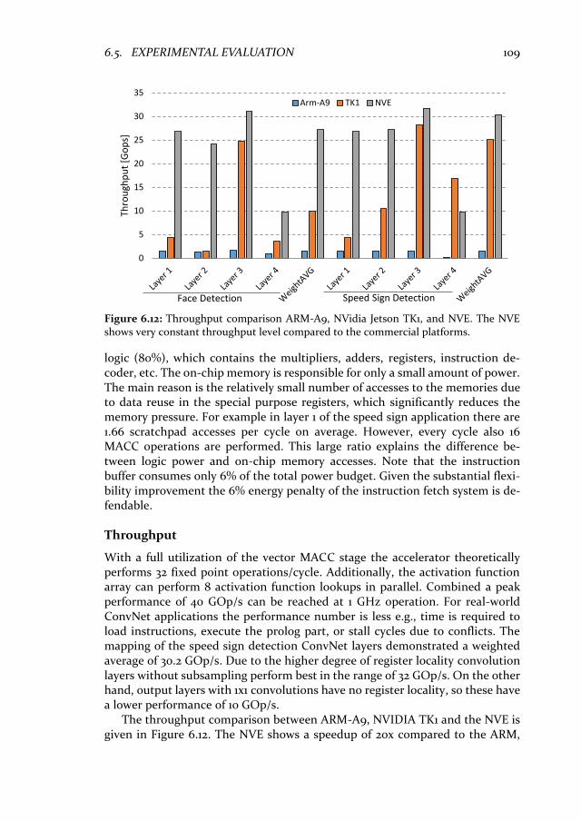
6.5. EXPERIMENTAL EVALUATION 109
logic (80%), which contains the multipliers, adders, registers, instruction de-coder, etc. The on-chip memory is responsible for only a small amount of power. The main reason is the relatively small number of accesses to the memories due to data reuse in the special purpose registers, which significantly reduces the memory pressure. For example in layer 1 of the speed sign application there are 1.66 scratchpad accesses per cycle on average. However, every cycle also 16 MACC operations are performed. This large ratio explains the difference be-tween logic power and on-chip memory accesses. Note that the instruction buffer consumes only 6% of the total power budget. Given the substantial flexi-bility improvement the 6% energy penalty of the instruction fetch system is de-fendable.
Throughput
With a full utilization of the vector MACC stage the accelerator theoretically performs 32 fixed point operations/cycle. Additionally, the activation function array can perform 8 activation function lookups in parallel. Combined a peak performance of 40 GOp/s can be reached at 1 GHz operation. For real-world ConvNet applications the performance number is less e.g., time is required to load instructions, execute the prolog part, or stall cycles due to conflicts. The mapping of the speed sign detection ConvNet layers demonstrated a weighted average of 30.2 GOp/s. Due to the higher degree of register locality convolution layers without subsampling perform best in the range of 32 GOp/s. On the other hand, output layers with 1x1 convolutions have no register locality, so these have a lower performance of 10 GOp/s.
The throughput comparison between ARM-A9, NVIDIA TK1 and the NVE is given in Figure 6.12. The NVE shows a speedup of 20x compared to the ARM,
0
5
10
15
20
25
30
35
Thro
ugh
pu
t [G
op
s]
Arm-A9 TK1 NVE
Face Detection Speed Sign Detection
Figure 6.12: Throughput comparison ARM-A9, NVidia Jetson TK1, and NVE. The NVE shows very constant throughput level compared to the commercial platforms.
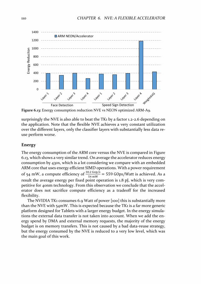
110 CHAPTER 6. NVE: A FLEXIBLE ACCELERATOR
surprisingly the NVE is also able to beat the TK1 by a factor 1.2-2.6 depending on the application. Note that the flexible NVE achieves a very constant utilization over the different layers, only the classifier layers with substantially less data re-use perform worse.
Energy
The energy consumption of the ARM core versus the NVE is compared in Figure 6.13, which shows a very similar trend. On average the accelerator reduces energy consumption by 430x, which is a lot considering we compare with an embedded ARM core that uses energy efficient SIMD operations. With a power requirement
of 54 mW, a compute efficiency of 30.2 Gop/s
54 mW= 559 GOps/Watt is achieved. As a
result the average energy per fixed point operation is 1.8 pJ, which is very com-petitive for 40nm technology. From this observation we conclude that the accel-erator does not sacrifice compute efficiency as a tradeoff for the increased flexibility.
The NVIDIA TK1 consumes 6.9 Watt of power [100] this is substantially more than the NVE with 54mW. This is expected because the TK1 is a far more generic platform designed for Tablets with a larger energy budget. In the energy simula-tions the external data transfer is not taken into account. When we add the en-ergy spend by DMA and external memory requests, the majority of the energy budget is on memory transfers. This is not caused by a bad data-reuse strategy, but the energy consumed by the NVE is reduced to a very low level, which was the main goal of this work.
0
200
400
600
800
1000
1200
1400En
ergy
Red
uci
ton
ARM NEON/Accelerator
Face Detection Speed Sign Detection
Figure 6.13: Energy consumption reduction NVE vs NEON optimized ARM-A9.

6.5. EXPERIMENTAL EVALUATION 111
6.5.3 Comparison against other ASIC accelerators
Researchers and computer architects nowadays recognize that the major im-provements in cost-energy-performance should come from domain specific hardware. This trend caused the introduction of many very new dedicated ASIC accelerators for ConvNet workloads. In Table 6.4 a number of ASIC based Conv-Net accelerators is compared to our default NVE configuration. We tried to ob-tain all accelerator characteristics, such as clock frequencies, technology node, and core voltages. Our proposed NVE accelerator has with only 16 MACC units less computational resources than the other comparison targets. For example, in the extreme there is a Tensor Processing Unit (TPU) [77] with 64k Multiply and Add units. The smallest accelerators are represented by Origami [15] and ShiDi-anNao [46], with 196 and 64 multipliers respectively.
The listed accelerators employ different techniques for parallelizing compu-tations. The NVE and ShiDianNao perform convolution in time and thereby maps computational resources to different output neurons. This makes utiliza-tion of the MACC units invariant to convolution window size. The other accel-erators such as DianNao and Origami, perform convolutions in space, so mapping computational resources to different pixels on the receptive fields of a neuron. Mapping convolutions in space makes the computational efficiency de-pendent on window size and negatively impacts utilization when the network parameters do not match the hardware.
The accelerator presented in [132] avoids most multiplications by performing lookups in a Q-table that contains pre-computed multiplication results. It uses a custom instruction set based controller that configures finite state machines on lower lever convolution cores. The chip presented in [43] contains multiple
Accelerator mW V Tech. MHz Gops Gops/ W
On-Chip Mem.
Con-trol
mm2 Gops/mm2
NeuFlow [110] 600 1.0 45 SOI 400 294 490 75 kB Data-flow
12.5 23.5
Origami [15] 93 0.8 umc 65 189 55 803 43 kB Config 1.31 42
NVE [109] 54 - TSMC 40
1000 30 559 20 kB VLIW 0.26 115
DianNao [20] 485 - TSMC 65
980 452 931 44 kB FSM 3.02 149.7
ShiDianNao [46]
320 - TSMC 65
1000 128* 400 288 kB FSM 4.86 26.3
Desoli et al. [43]
51 0.58 28 FD-SOI
200 78 1277 6 MB Config 34 2.29
Shin et al. [132]
35 0.77 65 1P8M 50 73 2100** 290 kB FSM 16 4.5
TPU [77] 40,000 - 28 nm 700 46,000 1150 28 MB CISC <331 >139
* Only gives theoretical peak performance, as opposed to actual measurements on a real network. ** Q-table lookup of precomputed multiplication results.
Table 6.4: Dedicated ASIC accelerator overview for ConvNets.

112 CHAPTER 6. NVE: A FLEXIBLE ACCELERATOR
DSP cores for general vision processing, a big on-chip memory, and a co-proces-sor subsystem with multiple convolution accelerators. The paper only lists power consumption for the co-processor, excluding on-chip memory. Control of the accelerator is handled through a set of configuration registers that configure a stream switch, allowing the reuse of data streams (similar to [16,110]).
The Tensor Processing Unit (TPU) [77] is a huge accelerator designed for server applications. The reported performance and power consumption are sev-eral orders of magnitude larger compared to the other designs, but still it is very efficient and makes good use of data reuse in the large on-chip memory. The control of a TPU is handled by complex high-level instructions that take multiple cycles to complete.
A computational throughput comparison of the accelerators shows that the NVE achieves 30 Gops, which is a relatively a low throughput. Note that the throughput numbers in Table 6.4 are the measured numbers that are given in the papers. The only exception is ShiDianNao [46] that only reports peak perfor-mance. Due to the large architectural differences it would be very interesting to simulate our real-world vision benchmarks on these architectures. Big accelera-tors such as a TPU are only well utilized if the workload fits their architecture. For instance the 256x256 Multiply Add array of a TPU would be completely un-derutilized when we map the Speed sign or Face detection workload. Underuti-lization effects would also occur for DianNao and Origami, because they use fixed convolution window sizes. Underutilization would substantially reduce the efficiency numbers of the other accelerator that are given in Table 6.4.
The NVE can perform layer merging technique as proposed in Chapter 4. For networks that support merging this results in a higher effective throughput. Our benchmark results in Figure 6.12 demonstrate that the NVE achieves a high uti-lization degree for different layers and convolution window configurations. One of the reasons is the VLIW based control model that also enables the use of op-timizing compilers. Important to note is that the NVE is by far the smallest de-sign and upon the three best designs regarding power consumption. These aspects make the NVE an excellent addition for ultra-low power systems on chip.
6.6 NVE instantiation and customization
During the evaluation a very flexible NVE instance is used. However the NVE is an accelerator template i.e., it is possible to modify the architecture at design time to specialize for different workloads. In this section an overview of some important configurations is given and the consequences of these modifications are discussed.
As demonstrated in Section 6.5.2 the largest component in silicon area (43%) is the local scratchpad memory. On the total energy budget the scratchpad con-sumes (11%). Different buffer configurations could reduce silicon area or energy consumption. For a quick exploration we evaluate 3 alternative memory config-urations:
6.6. NVE INSTANTIATION AND CUSTOMIZATION 113
1. Single port scratchpad, one load/store port 64-bit. 2. Simple dual port scratchpad, one load and one store port 64-bit. 3. Single port scratchpad, one load/store port 128-bit.
These configurations are compared against true dual port memory configuration (two load/store ports 64-bit wide) that maximizes flexibility. The 3x3 convolu-tion example from Figure 6.10 is used to evaluate the properties. The new sched-ules are given in Figure 6.14, Figure 6.15, and Figure 6.16.
The single port 64-bit wide memory (see Figure 6.14) has a clear memory bandwidth problem. The memory port is fully utilized and the vector MACC stage is stalling quite often. On the other hand, this single 64-bit ported memory has a significantly smaller silicon footprint, see Table 6.6. At the cost of a throughput reduction the NVE instantiation would shrink to 0.194 mm2, which is the smallest design. Because it is a single port design one of the AGUs can be removed, which reduces the power consumption. Table 6.5 shows that the single port memory consumes less power than others, but the energy efficiency is re-duced due to the low utilization of the vector MACC stage. A simple dual port configuration increases memory bandwidth. Although loads and stores can be performed concurrently the schedule in Figure 6.15 reveals that the load bandwidth is a performance bottleneck. Table 6.5 shows that the simple dual port memory is relatively large and has a lower energy efficiency. A further increase of scratchpad bandwidth is achieved by using a 128-bit wide single port memory. This configuration uses less silicon area w.r.t. the true dual port memory, and it offers similar data load bandwidth at a small flexibility penalty. According to Figure 6.9 single port loads of 128-bit require less energy per byte than any of the other configuration. However, the wide memory port loads re-quire more unnecessary data since the shift-in vector always contains 16 values that are fully utilized for convolutions with kernel windows of 16 elements. From the schedule in Figure 6.16 we conclude that throughput can be similar to the true dual ported configuration. However, the external input port should send more data into the accelerator due to the vector size inefficiency. The overview Table 6.5 shows that there is an energy efficiency advantage for the wide vector memory, over all other configurations. If we would take external memory energy into account this gain over the other configurations could be removed.

114 CHAPTER 6. NVE: A FLEXIBLE ACCELERATOR
Figure 6.14: Assembly schedule for a single port 64-bit wide scratchpad. Note that the VMACC stage is underutilized due to a bandwidth bottleneck with the scratchpad.
Figure 6.15: Assembly schedule for a simple dual port 64-bit wide scratchpad. The dedi-cated load port is a still a performance bottleneck for the VMACC issue slot.
Figure 6.16: Assembly schedule for a single port 128-bit wide scratchpad. The VMAC issue slot can be fully utilized since there is enough memory bandwidth to the scratchpad.
1
2
3
4
5
6
7
8
9
10
Cycle
11
12
13
14
15
st [s(i+2) word0]
ld [s(i+2) word0]
MEM port A
ld [b w0 w1 - ]
ld [s(i+0) word0]
st [s(i+2) word1]
ld [w2 w3 w4 -]
ld [s(i+1) word0]
st [s(i+2) word2]
ld [w5 w6 w7 w8]
ld [s(i+0) word1]
ld [s(i+0) word2]
ld [s(i+1) word1]
ld [s(i+1) word2]
ld [s(i+2) word1]
ld [s(i+2) word2]
shift
Weight REG
set [b w0 w1 -]
shift
shift
set [w5 w6 w7 w8]
set [w2 w3 w4 -]
shift
shift
shift
shift
shift
Image REG
set r0
set r2 shift
shift
shift
set r2 shift
set r0
set r2 shift
set r1
set r1
set r1
set r0
macc rw,ri
VMACC
set rw
macc rw,ri
macc rw,ri
macc rw,ri
macc rw,ri
macc rw,ri
macc rw,ri
macc rw,ri
macc rw,ri
act [s(i-1) word0]
act [s(i-1) word1]
VACT
1
2
3
4
5
6
7
8
9
10
Cycle
11
12
13
st [s(i+2) word0]
ld [s(i+2) word0]
MEM port Ald [b w0 w1 w2]
ld [s(i+0) word0]st [s(i+2) word1]
ld [w3 w4 w5 -]
ld [s(i+1) word0]
st [s(i+2) word2]
ld [w6 w7 w8 -]
ld [s(i+0) word1]
ld [s(i+0) word2]
ld [s(i+1) word1]
ld [s(i+1) word2]
ld [s(i+2) word1]
ld [s(i+2) word2]
Weight REG Image REG VMACC VACTMEM port B
shift
set [b w0 w1 -]
shift
shift
set [w5 w6 w7 w8]
set [w2 w3 w4 -]
shift
shift
shift
shift
shift
set r0
set r2 shift
shift
shift
set r2 shift
set r0
set r2 shift
set r1
set r1
set r1
set r0
macc rw,ri
set rw
macc rw,ri
macc rw,ri
macc rw,ri
macc rw,ri
macc rw,ri
macc rw,ri
macc rw,ri
macc rw,ri
act [s(i-1) word0]
act [s(i-1) word1]
1
2
3
4
5
6
7
8
9
10
Cyclest [s(i+2) word0]
ld [s(i+2) word0]
MEM port A
ld [b w0 - w4]
ld [s(i+0) word0]
st [s(i+2) word1]
ld [s(i+1) word0]
ld [w6 w7 w8 -]
ld [s(i+0) word1]
ld [s(i+1) word1]
ld [s(i+2) word1]
Weight REG Image REG VMACC VACTMEM port B
set [b w0 - w4]
shift
shift
set [w5 w6 w7 w8]
shift
shift
shift
shift
set r0
set r1, shift
shift
shift
set r0
set r1, shift
set r1, shift
set r0
macc rw,ri
set rw
macc rw,ri
macc rw,ri
macc rw,ri
macc rw,ri
macc rw,ri
macc rw,ri
macc rw,ri
macc rw,ri
act [s(i-1) word0]
act [s(i-1) word1]
shift
shift
shift

6.6. NVE INSTANTIATION AND CUSTOMIZATION 115
6.6.1 Limitations and future directions
As show by the short scratchpad memory exploration different trade-offs are possible in NVE configurations. Depending on the application set one could se-lect the perfect NVE instantiation at design time. A similar exploration could be done for the size of the vector MACC array. The 16 processing elements that are selected for this chapter are very well utilized for different workloads. Due to aggressive pipelining a clock speed of 1 Ghz is achieved that gives 32 Gop/s peak convolution performance. For some applications this is not enough, and one could evaluate larger vector arrays of 32, 64, or 128 MACC units. Note that the utilization of the vector MACC units will quickly decrease due to border effects. The NVE template really focusses at the ultra-low power domain below 100mW which will limits the wide vector scalability. Probably a multi-processor config-uration of NVE instances would give more flexibility and better scaling.
The current true dual ported implementation with 16 PEs achieves 13 fps real-time performance on the speed sign detection application. Wide vector imple-mentations or multi NVE accelerator configurations can certainly further im-prove on this performance. In addition, further work on the DMA engines is required. The NVE benefits a lot from streaming data that is well prepared for the architecture, e.g. packed coefficient vectors, or columns of feature map data. In [153] we developed a custom shuffling unit that can reorder and send the data vectors efficiently to the NVE accelerator. These Reordering Units are placed be-tween the memory interface controller and the NVE FIFO streams, as depicted in Figure 6.17. With larger memory structures these Reorder Engines could be used to exploit more data reuse over successive tile strips.
Table 6.5: NVE benchmark characteristics for the different scratchpad memory configu-rations while running the 3x3 convolution application.
Scratchpad config. Area [mm2] (%) Power [mW] (%) single port 64 bit 0.047 24% 3.445 6.7% simple dual port 64 bit 0.088 37% 4.397 8.6% single port 128 bit 0.070 32% 5.147 9.6% true dual port 64 bit 0.112 43% 5.926 10.9%
Scratchpad Config. Throughput Area NVE Power Gop/Watt pJ/Op single port 64 bit 21.3 Gop/s 0.194 mm2 45.3 mW 470 2.12 simple dual port 64 bit 24.5 Gop/s 0.235 mm2 50.6 mW 484 2.06 single port 128 bit 31.9 Gop/s 0.217 mm2 51.4 mW 621 1.61 true dual port 64 bit 31.9 Gop/s 0.259 mm2 54.1 mW 589 1.70
Table 6.6: Area and power consumption overview for different scratchpad configura-tions. All memories sizes are configured to have 8 Kbyte.

116 CHAPTER 6. NVE: A FLEXIBLE ACCELERATOR
6.7 Conclusions
Customized hardware acceleration for visual object classification has signifi-cantly improved the computational efficiency of Convolutional Networks (Conv-Nets). The current works are very specialized, which is often suboptimal for var-ying network configurations. We have presented a new SIMD architecture tem-plate for hardware-acceleration, the Neuro Vector Engine (NVE). In addition we demonstrated mapping and optimizations for inter-tile reuse to exploit the data locality optimizations from Chapter 5.
A VLIW-type of controller allows for sufficient flexibility to encode many ConvNet based machine vision applications. Synthesis on a low power 40 nm CMOS technology library resulted in a pipelined circuit that operates at 1 GHz, yielding an effective performance of 30.2 GOp/s on real benchmarks (20x faster w.r.t. a SIMD optimized ARM-A9). Considering the power budget of only 54 mW, this accelerator is suitable for embedment in the next-generation mobile devices and bring smart features like real-time visual object classification and speech recognition to our cherished portable companions.
Figure 6.17: Inter connection overview for a SoC equipped with an NVE instance.
DDR Memory
Memory Interface Controller
Host ProcessorARM core,MicroBlaze
Data Reorder Engine
Data Reorder Engine
NVE instance
FIFO streams
AXI4
AXI4Lite
Interrupt control
DDR IFOff-chip
On-chip
117
7.
ACCELERATOR CODE GENERATION
This chapter presents a compiler flow to map Deep Convolutional Networks (ConvNets) to highly specialized VLIW accelerator cores targeting the ul-tra-low power embedded market. Earlier works focused on energy efficient accelerators for this class of algorithms, but none of them provides a com-plete and practical programming model or a compiler. Due to the large pa-rameter set of ConvNets it is important that the user can abstract from the accelerator architecture and does not have to rely on an error prone and ad-hoc assembly programming model. By using automatic advanced code op-timization techniques such as data layout modification, modulo scheduling for software pipelining, and schedule combining for locality, we demon-strate that our compiler can produce highly optimized accelerator code. We evaluated our compiler on complex real-world vision applications with dif-ferent network layer configurations. The average throughput of our com-piler mapped applications is on-par with manual mappings by architecture experts that required multiple days of tuning. By combining multiple task schedules in ConvNet layers our compiler is able to reduce data transfers which is important for energy. More importantly our compiler solution re-duces the huge manual workload to efficiently map ConvNets to energy-efficient accelerator cores for the next-generation of mobile and wearable devices. This chapter is based on work presented at SCOPES 2015 [107].
7.1 Introduction
In Chapter 4, 5, and 6 we have shown that Convolutional Networks (ConvNets) have multiple computational challenges. Firstly, the computational workload in the number of operations is very high, which is addressed in Chapter 4 by con-volution and subsample merging. Secondly, the required data movement is a
CHAPTER

118 CHAPTER 7. ACCELERATOR CODE GENERATION
performance bottleneck and it consumes a lot of energy. The inter-tile reuse op-timization strategy from Chapter 5 reduces off-chip data transport a lot. Finally, we addressed the inefficiencies in general purpose computer architectures and existing accelerators in Chapter 6 by presenting the Neuro Vector Engine (NVE), a VLIW based accelerator that relies on vector operations.
Our community is well aware of the fact that architecture specialization is often required to achieve the best performance at low energy [113]. Other re-search groups also exploited the customization paradigm to design highly spe-cialized, and thus highly efficient cores that enable excellent machine vision for mobile devices [16,50,20,37,46]. These cores achieve most of their efficiency gains by tuning data storage structures to the dataflow and data-locality require-ments of the algorithm. The main challenge in accelerator design is to improve efficiency by architecture specialization, but maintain the flexibility. Especially, this flexibility is key for adoption of a new core. ConvNets have many parameters such as the number and type of layers, feature maps, and kernels, which are dif-ferent for every task. Hence the architecture should support different parameter combinations efficiently and it should have a programming model. A program-ming model can be an Instruction Set Architecture (ISA), or a configurable state machine. The NVE architecture is designed to be flexible in multiple ways: 1. A NVE is customizable such that it can be tuned at design time to match the user needs; 2. It achieves high data path utilization for many ConvNet workloads, so it is workload flexible; 3. It has the flexibility of being fully programmable; by loading an instruction sequence it can execute a different ConvNet.
Most earlier works focus on efficiently implementing compute primitives, but none provides a flexible architecture template. Additionally, these published architectures do not have a practical programming model or a compiler. They voluntarily ignore programming for simplicity [16], or they refer to an ad-hoc and therefore impractical assembly program [20,37], or a restrictive state ma-chine [46]. Only the Neuflow work [50] has a compiler model, but for this in-stance the architecture is very dedicated to a single network operator size.
In this chapter we present CONVE: a COmpiler for Neuro Vector Engines. To the best of our knowledge this is the first ConvNet compiler for a flexible accel-erator template such as, the Neuro Vector Engine [109] see Chapter 6. The auto-matic CONVE flow replaces the complicated and error prone task of manual assembly writing by a network specification in our Design Specific Language (DSL). This DSL is compiled into optimized VLIW assembly programs. This in-creases another degree of efficiency which is the mapping efficiency, i.e. the time and energy required to obtain an efficient mapping. Often the quality of gener-ated code is far lower than manually tuned code. However the performance on our compiled benchmark applications is slightly better than code optimized for days by architecture experts. The main contributions of this chapter are:
• Building a flexible VLIW compilation flow from a high level .json net-work description to assembly output.

7.2. BACKGROUND AND RELATED WORK 119
• A new bottom-up list scheduling approach that can be adapted for dif-ferent accelerator instantiations.
• New optimization steps: o Data layout modification to resolve resource conflicts; o Automatic modulo software pipelining to increase utilization; o Schedule combining to maximize performance and increase
data locality.
• An in-depth evaluation against manual written assembly code that’s written by architecture experts by using real-world ConvNet vision ap-plications.
This chapter is organized as follows: Section 7.2 gives an overview of related work in the field of compilers for accelerators and ConvNets. Section 7.3 introduces our Domain Specific Language (DSL) to specify network configurations for CONVE. Section 7.4 presents the CONVE code generation flow, and Section 7.5 discusses the advanced code optimization steps. In Section 7.6 we present an in-depth evaluation of the compiler results. Finally, Section 7.7 ends this chapter with conclusions.
7.2 Background and related work
Dedicated application accelerators are commonly used to process the dedicated workloads of different application domains. For example, our smartphones, dig-ital (video) cameras, and tablets all capture and process high-resolution images or video with a power constrained compute platform. Performing the compli-cated real-time processing tasks on high rate pixel streams require fixed function accelerators. Often these accelerators have limited flexibility, so no support for different coding standards or data processing steps. Much more flexibility is achieved with software defined solutions, such as a Digital Signal Processor (DSP), and Image Signal Processor (ISP), or techniques to enable Software De-fined Radios. In these cases programmable solutions are used which are more flexible and able to perform multiple tasks (better silicon efficiency). In addition, flexible cores can implement new functionalities or support new standards with a simple firmware update.
The NVE is a similar flexible signal processor specialized at ConvNet work-loads. The NVE template uses concepts from Very Long Instruction Word (VLIW) [52] based processors. The VLIW approach is popular among commer-cial DSPs e.g., the Tensilica Xtensa [57], or Silicon Hive [135] processor, or the more recent Qualcomm Hexagon [33] DSP; al are used in high end smartphones. A VLIW puts the complex scheduling responsibility for instruction level paral-lelism into a compiler and thereby avoids costly and power-hungry dynamic-scheduling hardware. By moving the complicated scheduling to a compiler the processor can be rather simple while it is able to achieve high performance. However, compiling efficient code for a general purpose VLIW core is challeng-

120 CHAPTER 7. ACCELERATOR CODE GENERATION
ing. The compilation challenges make that it is difficult to map applications ef-ficiently; as a result the programmer has to optimize his code manually or accept a bad hardware utilization. In conclusion, VLIW cores require a good optimizing compiler, otherwise the programmer must spend a tremendous effort in map-ping applications.
The CONVE compiler focusses on ConvNets, so the input programs have a regular structure. By narrowing the group of target applications compilation and optimization becomes more specific. As a result, more effort is spend in compi-lation routines that produce code that achieve close to peak performance on the NVE template without manual tuning.
Next to the general purpose VLIW base accelerator DSP cores there are many fixed function cores focussing on ConvNets. However most of them are less flex-ible compared the NVE template. These works mainly focus on the convolution operations, but programmability or efficient code generation are out of the scope or simply neglected. Some exceptions do exist, for instance the NeuFlow [50] dataflow architecture which uses a software API called LuaFlow. Their flow con-verts descriptions, using Torch [34] into dataflow programs. In Torch ConvNets are specified layer-by-layer, each with parameters such as kernel size, subsample factor, number of inputs, and number of outputs for each layer. However, Torch lacks the freedom to assign a custom feature map connectivity. Only several con-nection types are allowed, e.g. fully connected, one-to-one, or random. For our vision benchmarks this would be too restrictive and forcing us to make many extra connections with coefficient values set to zero. In addition, the operators are specified as systolic array streams, which are underutilized if multiple vary-ing kernel sizes are used.
Another recent fixed function accelerator program flow is used in the ShiDi-anNao [46] work. ConvNets are described as a Hierarchical Finite State Machine (FSM), see Figure 7.1. Two hierarchical FSM levels are used where the first de-scribes the high-level flow through the network and the second controls low-
S6 S7
S1
S2S3
S4
S5S0
matrix others
conv.
pooling
classifier
ALU
square
s10 s11
s12s13
s14
s15
idle init
h-modev-mode
fill
finish
start
load
one row
next window
next row
finish
First-Level States Second-Level States
Figure 7.1: Hierarchical control finite state machine of the ShiDianNao accelerator.

7.3. CONVNETS IN A DOMAIN SPECIFIC LANGUAGE 121
level details, e.g., the operation patterns of convolution or pooling. This ap-proach replaces the use of instructions by FSM parameters, but these are less flexible and limited by the number of FSM states. For the FSM there is no high-level language, so programmers must create their own low-level FSM parameters to express each new network. Note that while the ShiDianNao accelerator has worked out an energy efficient control mechanism other key works still neglect this very important part. For example, the very recent and detailed Eyeriss pub-lications [22,21] do not discuss their control architecture or input code genera-tion. These papers present an in-depth study on data movement patterns and compute workload. For some reason the control architecture is left out and also input code generation is not covered. We argue that control and input code are key parts to improve the efficiency of an accelerator core. Therefore we discuss the details of building an application specific compiler. Firstly, the challenge that must be overcome is to generate code that achieves high accelerator utilization. Secondly, the mapping process needs to be simplified for applications on accel-erators or improving the programmer’s productivity, which is also an efficiency.
7.3 ConvNets in a domain specific language
As shown in the previous section many related ConvNet accelerators do not dis-cuss their method of programming network parameters into their design. On the opposite there are also general purpose accelerator cores that use the C lan-guage with advanced compilers. These cores often struggle with the wide range of input programs for which always valid machine code should be generated. The CONVE framework takes a more abstract approach by relying on a Domain Specific Language (DSL) for ConvNets.
Our DSL is based upon the network description format fort he popular soft-ware library Caffe [76]. Caffe is used to train Deep ConvNets with consumer hardware like GPUs. It brings the complicated training algorithms that are used for Deep Learning to the mass public. Their input description is based on .json, an open-standard format that uses human-readable text to define data objects. By default their language assumes full connectivity between feature maps, but the connectivity can be split with “group” parameters. These “group” parameters do not support the specification of custom layer-to-layer connectivity, which is important for workload reduction. Therefor we modified the CONVE input lan-guage such that users are able to express custom networks with sparse feature map connectivity. Furthermore, our CONVE input format is restrictive to Conv-Net workloads such that unsupported program flows are prevented. This makes it much simpler to generate correct code from our DSL input.
Caffe trained networks can be easily mapped to our platform, since both de-scription languages are very similar. The main difference is the flexibility to use connectivity patterns that are supported by the NVE. These sparse maps are key for efficient processing, since it substantially reduces the workload. Listing 7.1 gives an example description for the first and second layer of the face detection

122 CHAPTER 7. ACCELERATOR CODE GENERATION
benchmark. First an application (name) is specified and then the network (lay-ers). Each layer has a descriptor which lists parameters such as output size (output.size), activation function (output.act), output mapping (out-put.map), kernel size (kernel.size), pooling size (kernel.pool.size), and pooling kernel type (kernel.pool.type).
7.4 Automatic code generation flow
This section presents our automatic code generation flow in detail. As illustrated by Figure 7.2 the flow starts with a high-level ConvNet input description (Section 7.3). This description is converted into a separate task graph for each output fea-ture map (Section 7.4.1). The taskgraph can be optimized by coefficient repack-ing (Section 7.5.1) The instruction scheduling step constructs a schedule for every graph (Section 7.4.2). Further optimization steps are performed: e.g. mod-ulo scheduling to increase utilization (Section 7.5.2); and combine feature map schedules to improve locality (Section 7.5.3). Physical buffer space is assigned for
{ "name": "Face Detector", "layers": [{ "output": {"size": [638,358],"act": "sigm", "map": [ [0,1,2,3] ] }, "kernel": {"size": [6,6],"pool": {"size": [2,2],"type": "avg"}} }, { "output": {"size": [317,177], "act": "sigm", "map": [ [0,1,8,11,13], [2,3,8,9,12], [4,5,9,10,11], [6,7,10,12,13] ] }, "kernel": {"size": [4,4],"pool": {"size": [2,2],"type": "avg"}} }] }
Listing 7.1: JSON Convolutional network description of first and second layer of the face detection benchmark workload.
Task Graph Generation
Instruction Scheduling
Buffer Allocation
.json ConvNet
VLIW program
Assembling
Coefficient Packing
Schedule Combining
Modulo Scheduling
Added optimization
steps
Normal flow
Figure 7.2: The CONVE automatic NVE code generation flow.

7.4. AUTOMATIC CODE GENERATION FLOW 123
the schedules (Section 7.4.3), and finally these are converted into executable bi-naries for the VLIW instruction memory.
7.4.1 Task graph construction
The first step of the VLIW code generation is to represent the network layers as task graph or a Direct Acyclic Graph (DAG). These graphs are constructed by tracing back through the computation sequence for neuron outputs. This is per-formed by our graph constructor that creates a DAG from the .json input de-scription. The graph is constructed by applying the structure rules of a ConvNet. The details of construction are discussed by an educational example of a 3x3 fil-ter application.
Convolution outputs of 3x3 kernels require 9 MACC and one set bias initial-ization. In addition, these operations require coefficients, e.g., one bias, and 9 weight values that are broadcasted to the MACC vector unit, recall Figure 6.7. The weight register loads a word of four 16-bit coefficients (full capacity). The first entry is broadcasted directly after the load and the others by shift opera-tions. As a result, three weight register set, and 7 shift operations are instan-tiated. The corresponding image data must be loaded in the image registers.
sh rw
setsh
ri
macc
set ri
ld
set b
set rw
ld
st
st
macc
set b
1
1
set ri
set rw
macc
set b
1
1
1
sh rw
1
1
1
sh rw
1
sh rw
setsh
ri
set ri
set rw
macc
set b
1
1
1
1
1
sh rw
1
0
00
sh rw
setsh
ri
set ri
set rw
macc
set b
1
1
1
1
1
sh rw
1
0
00
2 2
2
2
connectanti-dependencies
connectread & write operations
connectregister-mac dependencies
connectregister dependencies
define computations
ld
st
2
2
Figure 7.3: Direct Acyclic Graph (DAG) construction for computation of an output fea-ture map.

124 CHAPTER 7. ACCELERATOR CODE GENERATION
Depending on the number of MACCs, pooling stride, and kernel shape a se-quence of image register operations is selected. For 3x3 convolution the se-quence is: set, set shift, and shift which is repeated for each column. The register set operations require loads from the scratchpad memory e.g., for weights three loads from port A. A register set on the image register re-quires two loads (port A and B) to fill position 0-15. The image register set and shift operation require a single load from port B, which fills the shift-in regis-ter. The small example requires 9 scratchpad loads for image data per group of 16 neurons. In case of a pooling factor a different set of image registers is used that require four loads to fill the larger image vector.
Operations in a task graph or Direct Acyclic Graph (DAG) must be connected with their dependencies, e.g., a set bias occurs before the first MACC operation so a dependence is connected, see Figure 7.3 (top-left). MACC operations require data from registers, so dependence arrows from register operations are con-nected (topmiddle). Successive register shift operations are connected, since they depend on the previous value (top-right); Anti-dependencies from MACCs to the registers are added as depicted in Figure 7.3 (bottom-left). These anti-dependencies ensure that the weights and pixels are not overwritten before the associated MACC operation takes place. Finally, dependencies between reg-ister set operations and scratchpad load operations are connected (bottom-right). A load has a dependency to a preceding store operations. All depend-encies have a distance parameter representing the minimum latency between adjacent vertices. A simplified task graph construction pseudo description is given in Algorithm 8.1.
ALGORITHM 8.1: Direct Acyclic Graph (DAG) construction for an output feature map input: kernel size 𝑘𝑥 and 𝑘𝑦, subsample 𝑝𝑥 and 𝑝𝑦, number of inputs 𝑝
output: graph 𝐺(𝑣, 𝑒) 1 graph 𝐺; 2 vertex 𝑣; 3 𝑣 ←set bias; //initialize neurons 4 insert_vertex(𝑣, 𝐺); 5 for 𝑖 < 𝑘𝑥 ∗ 𝑘𝑦 do
6 𝑣 ←MACC; //process neuron inputs 7 insert_vertex(𝑣, 𝐺); 8 end 9 create dependencies between set bias and first MACC vertices in 𝐺; 10 for 𝑖 < 2 do 11 𝑣 ← activation; //two acts per vector for this NVE instance 12 insert_vertex(𝑣, 𝐺); 13 insert_dep(𝑣setbias, 𝑣, 𝐺); 14 end 15 for 𝑖 < 𝑛 ∗ 𝑘𝑥 ∗ 𝑘𝑦 do
16 if 𝑖%𝑘𝑦 = 0 then
17 𝑣 ← set ri; //each ky a set register 18 else if 𝑖%𝑘𝑦 = 1 then
19 𝑣 ← set shift ri; //load the shift-in register

7.4. AUTOMATIC CODE GENERATION FLOW 125
20 else if then 21 𝑣 ← shift ri; //shift the image registers 22 insert_vertex(𝑣, 𝐺); 23 end 24 create dependencies between set ri and following shift ri vertices in 𝐺; 25 create dependencies between shift ri and following shift ri vertices in 𝐺; 26 create dependencies between MACC and adjacent ri vertices in 𝐺; 27 create dependencies between ri operations with adjacent MACC in 𝐺; 28 PackCoefficients() ; //see section 7.5.1 29 foreach set ri/rw in 𝐺 do 30 𝑣 ← ld ri/rw; //load operation from local scratchpad 31 insert_vertex(𝑣, 𝐺) 32 𝑣 ← st ri/rw; //store operation into local scratchpad
33 insert_vertex(𝑣, 𝐺); 34 end 35 foreach ld ri/rw in 𝐺 do 36 insert_dep(𝑣ld, 𝑣set, 𝐺); //connect load and set registers 37 end 38 foreach st ri/rw in 𝐺 do 39 insert_dep(𝑣st, 𝑣ld, 𝐺); //connect store and load operations 40 end
7.4.2 Instruction scheduling
A task graph alone cannot be executed by our accelerator. It is an intermediate representation for the operations with their dependency constraints. This graph must be converted into operations that are timed in the VLIW slots. Algo-rithm 8.2 describes our custom list scheduling procedure that works bottom up through the graph. At the bottom there exist a single root where at top multiple start vertices should be evaluated. Breadth First Search (BFS) is used to visit and schedule vertices with a complexity of 𝑂(𝑉 + 𝐸). For example, BFS starts by add-ing the bottom vertex (𝑥) of task graph (𝐺) to a queue (𝑄) then all parents of (𝑥) are visited one-by-one. During a visit, a time slot (𝑡) is assigned to the visited parent vertices (𝑤), these time slots are based on the time slots of child vertices (𝑣) and distance (𝑑).
In Figure 7.4 the scheduling procedure is demonstrated on the 3x3 filter ex-ample. First, time slot 0 is assigned to the bottom vertex. By applying BFS time slots are assigned bottom-up to the parent nodes based upon the dependence distances. The required resources are claimed, however in some cases these are already occupied which causes a delay slot in the schedule. For example, a bit further in the graph a MACC operation is assigned to slot (-5). The connected parent nodes (see dashed nodes in Figure 7.4) require a set weight (set rw) and a set image register (set ri) operation. The scratchpad memory port con-straints allow only one of the two set register operations at a time. As a result, the first visited (set rw) is assigned to slot -6. In the set register resource table slot -6 is claimed, see Figure 7.5. When the other parent node is visited a conflict
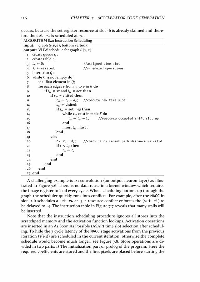
126 CHAPTER 7. ACCELERATOR CODE GENERATION
occurs, because the set register resource at slot -6 is already claimed and there-fore the set ri is scheduled at -7.
ALGORITHM 8.2: Instruction Scheduling input: graph 𝐺(𝑣, 𝑒), bottom vertex 𝑥 output: VLIW schedule for graph 𝐺(𝑣, 𝑒)
1 create queue 𝑄; 2 create table 𝑇; 3 𝑡𝑥 ← 0; //assigned time slot 4 𝑠𝑥 ← visited; //scheduled operations 5 insert 𝑥 to 𝑄; 6 while 𝑄 is not empty do; 7 𝑣 ← first element in 𝑄; 8 foreach edges 𝑒 from 𝑤 to 𝑣 in 𝐺 do 9 if 𝑖𝑤 ≠ st and 𝑖𝑤 ≠ act then 10 if 𝑠𝑤 ≠ visited then 11 𝑡𝑤 ← 𝑡𝑣 − 𝑑𝑒; //compute new time slot 12 𝑠𝑤 ← visited; 13 if 𝑖𝑤 = set reg then 14 while 𝑡𝑤 exist in table 𝑇 do 15 𝑡𝑤 ← 𝑡𝑤 − 1; //resource occupied shift slot up 16 end 17 insert 𝑡𝑤 into 𝑇; 18 end 19 else 20 𝑡 ← 𝑡𝑣 − 𝑑𝑒; //check if different path distance is valid
21 if 𝑡 < 𝑡𝑤 then 22 𝑡𝑤 ← 𝑡; 23 end 24 end 25 end 26 end 27 end
A challenging example is 1x1 convolution (an output neuron layer) as illus-trated in Figure 7.6. There is no data reuse in a kernel window which requires the image register to load every cycle. When scheduling bottom-up through the graph the scheduler quickly runs into conflicts. For example, after the MACC in slot -2 it schedules a set rw at -3, a resource conflict enforces the (set ri) to be delayed to -4. The instruction table in Figure 7.7 reveals that many stalls will be inserted.
Note that the instruction scheduling procedure ignores all stores into the scratchpad memory and the activation function lookups. Activation operations are inserted in an As Soon As Possible (ASAP) time slot selection after schedul-ing. To hide the 3 cycle latency of the MACC stage activations from the previous iteration (s(i-1)) are scheduled in the current iteration, otherwise the complete schedule would become much longer, see Figure 7.8. Store operations are di-vided in two parts: 1) The initialization part or prolog of the program. Here the required coefficients are stored and the first pixels are placed before starting the
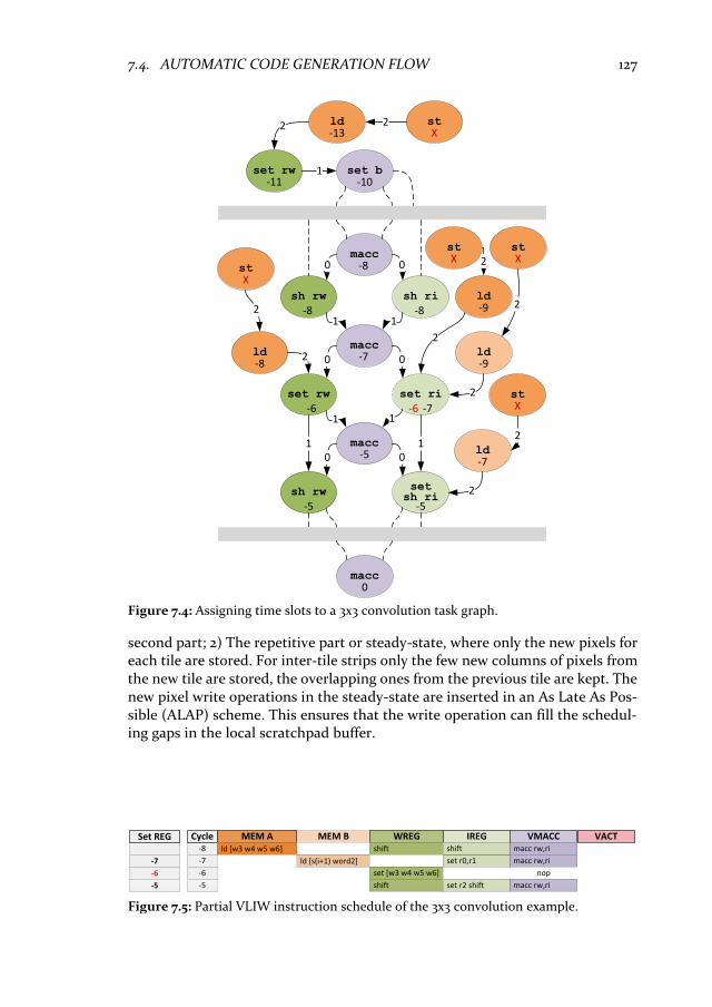
7.4. AUTOMATIC CODE GENERATION FLOW 127
second part; 2) The repetitive part or steady-state, where only the new pixels for each tile are stored. For inter-tile strips only the few new columns of pixels from the new tile are stored, the overlapping ones from the previous tile are kept. The new pixel write operations in the steady-state are inserted in an As Late As Pos-sible (ALAP) scheme. This ensures that the write operation can fill the schedul-ing gaps in the local scratchpad buffer.
sh rw sh ri
sh rwsetsh ri
macc
macc
macc
set rw set ri
0 0
11
00
11
1 100
ld
ld
ld
2
2
2
-5-5
-5
-6 -6 -7
-8-7
-9
-9
-8
-8
-8
macc0
set bset rw 1
ld2
st
2
st
2st
2
st2
X
X X
X
-10-11
-13
ld
2
-7
st
2
X
Figure 7.4: Assigning time slots to a 3x3 convolution task graph.
MEM B
ld [s(i+1) word2]
set [w3 w4 w5 w6]
WREG
shift macc rw,ri
VMACCmacc rw,ri
macc rw,ri
MEM A VACTshift-8
-7
-6
-5
Cycle IREG
set r0,r1
shift
set r2 shift
nop
ld [w3 w4 w5 w6]
-7
-6
-5
Set REG
Figure 7.5: Partial VLIW instruction schedule of the 3x3 convolution example.
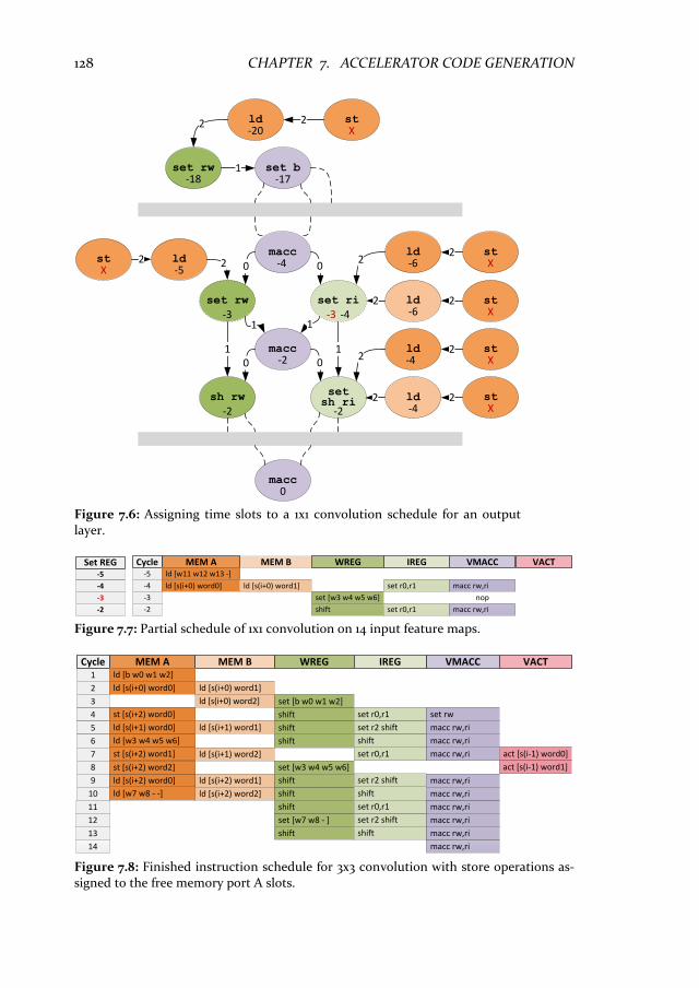
128 CHAPTER 7. ACCELERATOR CODE GENERATION
Figure 7.8: Finished instruction schedule for 3x3 convolution with store operations as-signed to the free memory port A slots.
sh rwsetsh ri
macc
macc
set rw set ri
00
11
1 100
ldld
ld
2
2
2
-2-2
-2
-3 -3 -4
-5-4 -6
-6
macc0
set bset rw 1
ld2
st 2st2
st2
st2
XX
X
X
-17-18
-20
ld2-4
st2X
ld-42
st2X
MEM B
ld [s(i+0) word1]
set [w3 w4 w5 w6]
WREG
shift macc rw,ri
VMACC
macc rw,ri
MEM A VACT-5
-4
-3
-2
Cycle IREG
set r0,r1
set r0,r1
nop
ld [w11 w12 w13 -]-5
-4
-3
-2
Set REG
ld [s(i+0) word0]
st [s(i+2) word0]
ld [s(i+2) word0]
MEM B
ld [s(i+0) word1]
shift
WREG
set [b w0 w1 w2]
shift
macc rw,ri
VMACC
set rw
macc rw,ri
macc rw,ri
macc rw,ri
shift
set [w7 w8 - ]
set [w3 w4 w5 w6]
ld [s(i+1) word1]
ld [s(i+0) word2]
shift
shift
macc rw,ri
macc rw,ri
macc rw,rishift
ld [s(i+2) word1]
MEM A VACT
act [s(i-1) word0]
act [s(i-1) word1]
ld [s(i+2) word2]
shift
ld [s(i+1) word2]
1
2
3
4
5
6
7
8
9
10
Cycleld [b w0 w1 w2]
ld [s(i+0) word0]
st [s(i+2) word1]
ld [w3 w4 w5 w6]
ld [s(i+1) word0]
st [s(i+2) word2]
ld [w7 w8 - -]
shift
IREG
set r0,r1
set r2 shift
shift
shift
set r2 shift
set r0,r1
set r2 shift
set r0,r1
macc rw,ri
macc rw,ri
11
12
13
14
Figure 7.6: Assigning time slots to a 1x1 convolution schedule for an output layer.
Figure 7.7: Partial schedule of 1x1 convolution on 14 input feature maps.
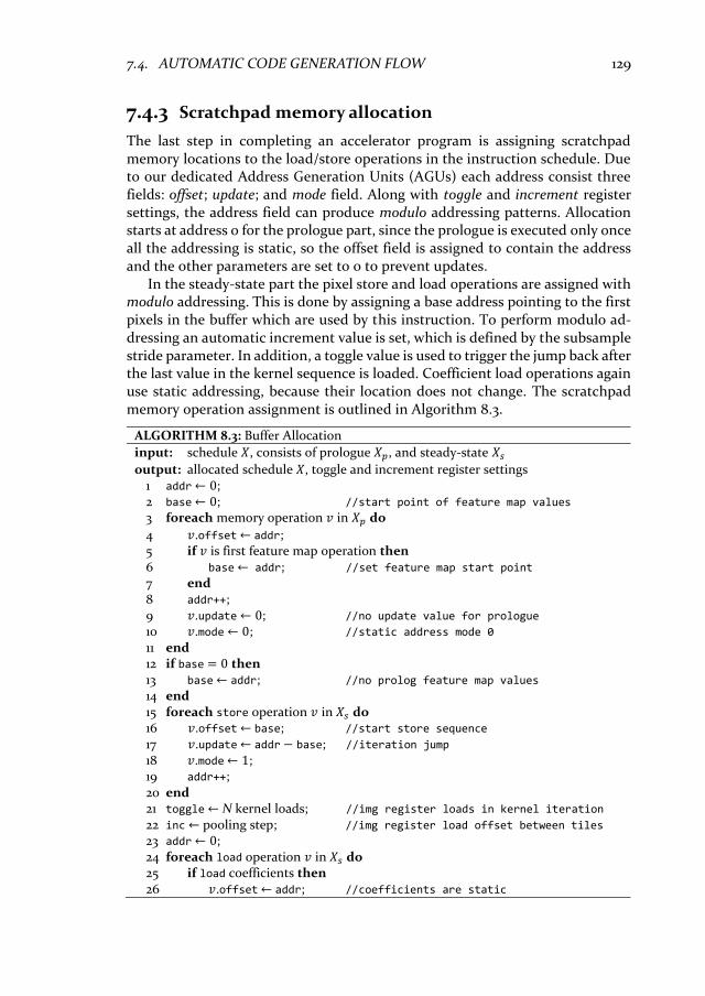
7.4. AUTOMATIC CODE GENERATION FLOW 129
7.4.3 Scratchpad memory allocation
The last step in completing an accelerator program is assigning scratchpad memory locations to the load/store operations in the instruction schedule. Due to our dedicated Address Generation Units (AGUs) each address consist three fields: offset; update; and mode field. Along with toggle and increment register settings, the address field can produce modulo addressing patterns. Allocation starts at address 0 for the prologue part, since the prologue is executed only once all the addressing is static, so the offset field is assigned to contain the address and the other parameters are set to 0 to prevent updates.
In the steady-state part the pixel store and load operations are assigned with modulo addressing. This is done by assigning a base address pointing to the first pixels in the buffer which are used by this instruction. To perform modulo ad-dressing an automatic increment value is set, which is defined by the subsample stride parameter. In addition, a toggle value is used to trigger the jump back after the last value in the kernel sequence is loaded. Coefficient load operations again use static addressing, because their location does not change. The scratchpad memory operation assignment is outlined in Algorithm 8.3.
ALGORITHM 8.3: Buffer Allocation input: schedule 𝑋, consists of prologue 𝑋𝑝, and steady-state 𝑋𝑠
output: allocated schedule 𝑋, toggle and increment register settings 1 addr ← 0; 2 base ← 0; //start point of feature map values 3 foreach memory operation 𝑣 in 𝑋𝑝 do
4 𝑣.offset ← addr; 5 if 𝑣 is first feature map operation then 6 base ← addr; //set feature map start point 7 end 8 addr++; 9 𝑣.update ← 0; //no update value for prologue
10 𝑣.mode ← 0; //static address mode 0 11 end 12 if base = 0 then 13 base ← addr; //no prolog feature map values 14 end 15 foreach store operation 𝑣 in 𝑋𝑠 do 16 𝑣.offset ← base; //start store sequence 17 𝑣.update ← addr − base; //iteration jump 18 𝑣.mode ← 1; 19 addr++; 20 end 21 toggle ← N kernel loads; //img register loads in kernel iteration 22 inc ← pooling step; //img register load offset between tiles 23 addr ← 0; 24 foreach load operation 𝑣 in 𝑋𝑠 do 25 if load coefficients then 26 𝑣.offset ← addr; //coefficients are static
130 CHAPTER 7. ACCELERATOR CODE GENERATION
27 𝑣.update ← 0; //no updating of addresses 28 𝑣.mode ← 0; 29 addr++; 30 end 31 end 32 addr ← 0; 33 foreach load operation 𝑣 in 𝑋𝑠 do 34 if load feature map then 35 𝑣.offset ← base; //start load sequence 36 𝑣.update ← addr; 37 𝑣.mode ← 1; 38 addr++; 39 end 40 end
7.4.4 Generalization towards VLIW architecture
The CONVE compiler framework is designed with flexibility in mind. In case the instantiation of an NVE core changes (see parameters in Figure 6.7) small mod-ifications to the task graph construction procedure are required. These tech-niques are well-known from VLIW processor design e.g. Tensilica Xtensa [57] or the Silicon Hive [135] tools. For example, when instructions are added or re-moved the operators in the task graph should be changed accordingly based upon the new set of operations. Additionally, the dependencies among vertices can change based upon modifications in the processing pipeline. Instruction scheduling is adapted mainly in the resource conflict resolution scheme. For ex-ample, the use of a single port scratchpad memory changes the resource alloca-tion table.
The memory address allocation is rather specific due to the use of AGUs. In case the AGUs are removed addresses would be static which removes the huge advantages of inter-tile reuse patterns. Note that dedicated Caches could largely solve these issues at the cost of an area and energy penalty. Finally the transla-tion of a new instruction scheme into executable binaries is straight forward but it must comply with the VLIW slots of the architecture.
From this point onwards different architecture variants can be explored. Consider a case where the NVE instance has more scratchpad memory ports, e.g. a dedicated port assigned to each set register operation this to remove conflict nop operations. Another example would be doubling the size of the vector MACC unit, which will result in more image register operations in case the vector memory size of 8 byte is kept. All these alternatives could be explored in future work to find good performance/area/energy configurations.
7.5. ADVANCED CODE OPTIMIZATIONS 131
7.5 Advanced code optimizations
Compiling high-level program descriptions into correct assembly programs is essential for any accelerator. Without such tools mapping of complicated tasks would become almost impossible. Another aspect is the code quality, ideally it performs similar to a manual mapping. However, often an automatic compiler path generates low-quality code, reducing the energy and performance ad-vantages of dedicated architectures like the NVE. In this section we focus on advanced code optimizations to generate code that performs on-par with an ex-pert programmer.
Careful analysis of manual (Figure 6.10) and default compiler (Figure 7.8) generated schedules reveals that the later one reduces throughput by 1.4 times. Generated instruction schedules contain more NOP gaps due to resource con-flicts and idle time between steady-state iterations. Furthermore, there is no data locality optimization for shared inputs over output feature maps. The following optimizations sections will improve performance by addressing these three missing optimization steps.
7.5.1 Coefficient layout optimizations
Register load port sharing is one of the architecture constraints that sometimes inserts NOP gaps since the set register of a weight and image register cannot execute in the same cycle. The default compiler resolves such resource conflicts by delaying one of the operations, which causes a NOP in the VMACC slot. This is illustrated in the task graph of Figure 7.4 and the instruction schedule of Figure 7.5. An expert programmer resolves such conflicts by off-line altering coefficient layout of scratchpad vectors. As a result, a weight set and shift operation can be interchanged which often avoids the conflict and the inserted NOP. Our compiler uses a similar coefficient packing procedure in the task graph generation step that reduces the number of weights in a vector before a conflict occurs. This procedure imitates the manual optimization strategy. Note that this procedure does not always solve the conflicts, sometimes the upper load port is over-uti-lized. For example, in the 1x1 convolution benchmark there is no image register reuse and therefore every cycle a set register operation is requested. Without insertion of stalls there are simply no free slots to load the weight register (see Figure 7.6 and Figure 7.7). In these cases our compiler accepts the penalty and packs the weight vectors with the maximum number of weights.
7.5.2 Modulo scheduling
Modulo scheduling is implemented by measuring the Resource Minimum Initia-tion Interval (ResMII), which is defined by the issue slot that requires the longest sequence of execution cycles. The ResMII is used to wrap the schedule and con-
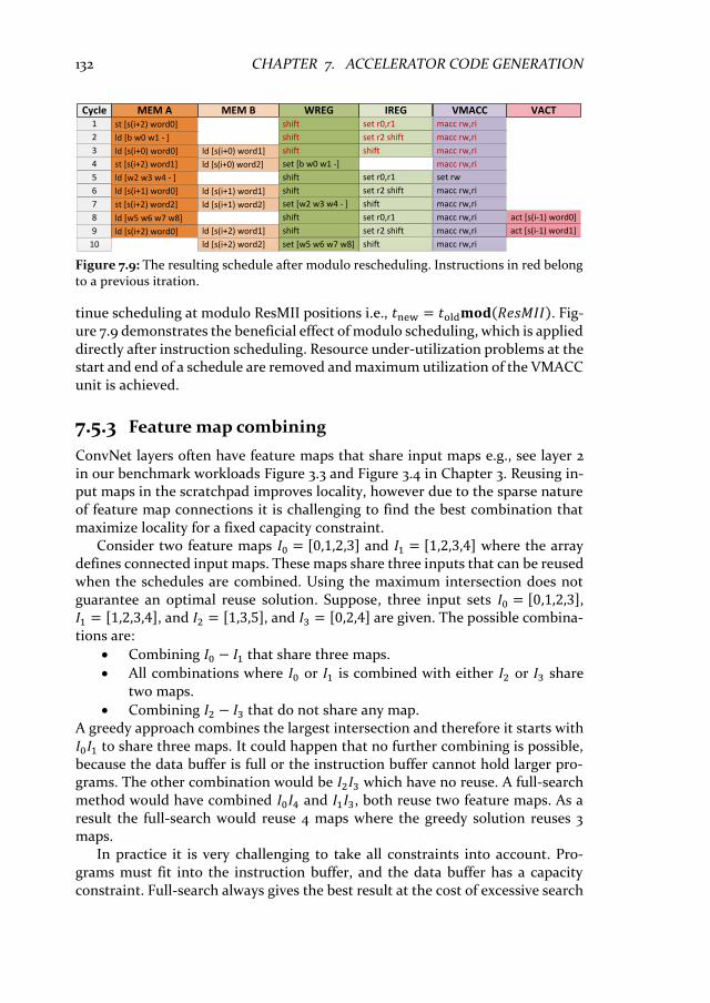
132 CHAPTER 7. ACCELERATOR CODE GENERATION
tinue scheduling at modulo ResMII positions i.e., 𝑡new = 𝑡old𝐦𝐨𝐝(𝑅𝑒𝑠𝑀𝐼𝐼). Fig-ure 7.9 demonstrates the beneficial effect of modulo scheduling, which is applied directly after instruction scheduling. Resource under-utilization problems at the start and end of a schedule are removed and maximum utilization of the VMACC unit is achieved.
7.5.3 Feature map combining
ConvNet layers often have feature maps that share input maps e.g., see layer 2 in our benchmark workloads Figure 3.3 and Figure 3.4 in Chapter 3. Reusing in-put maps in the scratchpad improves locality, however due to the sparse nature of feature map connections it is challenging to find the best combination that maximize locality for a fixed capacity constraint.
Consider two feature maps 𝐼0 = [0,1,2,3] and 𝐼1 = [1,2,3,4] where the array defines connected input maps. These maps share three inputs that can be reused when the schedules are combined. Using the maximum intersection does not guarantee an optimal reuse solution. Suppose, three input sets 𝐼0 = [0,1,2,3], 𝐼1 = [1,2,3,4], and 𝐼2 = [1,3,5], and 𝐼3 = [0,2,4] are given. The possible combina-tions are:
• Combining 𝐼0 − 𝐼1 that share three maps.
• All combinations where 𝐼0 or 𝐼1 is combined with either 𝐼2 or 𝐼3 share two maps.
• Combining 𝐼2 − 𝐼3 that do not share any map. A greedy approach combines the largest intersection and therefore it starts with 𝐼0𝐼1 to share three maps. It could happen that no further combining is possible, because the data buffer is full or the instruction buffer cannot hold larger pro-grams. The other combination would be 𝐼2𝐼3 which have no reuse. A full-search method would have combined 𝐼0𝐼4 and 𝐼1𝐼3, both reuse two feature maps. As a result the full-search would reuse 4 maps where the greedy solution reuses 3 maps.
In practice it is very challenging to take all constraints into account. Pro-grams must fit into the instruction buffer, and the data buffer has a capacity constraint. Full-search always gives the best result at the cost of excessive search
st [s(i+2) word0]
ld [s(i+2) word0]
MEM B
ld [s(i+0) word1]
shift
WREG
set [b w0 w1 -]
shift
macc rw,ri
VMACC
set rw
macc rw,ri
macc rw,ri
macc rw,ri
shift
set [w5 w6 w7 w8]
set [w2 w3 w4 - ]
ld [s(i+1) word1]
ld [s(i+0) word2]
shift
shift
macc rw,ri
macc rw,ri
macc rw,ri
shift
ld [s(i+2) word1]
MEM A VACT
act [s(i-1) word0]
act [s(i-1) word1]
ld [s(i+2) word2]
shift
ld [s(i+1) word2]
1
2
3
4
5
6
7
8
9
10
Cycle
ld [b w0 w1 - ]
ld [s(i+0) word0]
st [s(i+2) word1]
ld [w2 w3 w4 - ]
ld [s(i+1) word0]
st [s(i+2) word2]
ld [w5 w6 w7 w8]
shift
IREG
set r0,r1
set r2 shift
shift
shift
set r2 shift
set r0,r1
set r2 shift
set r0,r1
macc rw,ri
macc rw,ri
Figure 7.9: The resulting schedule after modulo rescheduling. Instructions in red belong to a previous itration.

7.5. ADVANCED CODE OPTIMIZATIONS 133
time for large layers. As a trade-off we implemented greedy feature map com-bining. For many layers our greedy scheduling finds a solution close to the opti-mum and is already much better than not combining at all.
Algorithm 8.4 lists our combining procedure, where 𝐿 holds individual schedules and 𝑅 a list of combined programs. First, it searches for the program with the largest number of input featuremaps. The selected featuremap is com-bined with another map that gives: 1) Minimizes the difference 𝛼 of input maps; 2) Obtain the largest intersection 𝛽. This repeats until the scratchpad buffer or the instruction buffer is filled and the program 𝑓 can be stored as a valid sched-ule. Next, the procedure repeats for the remaining featuremaps until all maps are stored. Featuremap combining is performed before modulo scheduling, since the modulo operation merges a program across iterations, which makes it diffi-cult to insert another featuremap. Combining featuremaps and afterwards per-forming modulo scheduling is much simpler and gives benefit of both optimizations. Note that modulo scheduling is tested after every new combina-tion to validate the instruction memory capacity constraint.
ALGORITHM 8.4: Feature Map Fusion input: list of individual feature map schedules 𝐿 output: list of combined schedules 𝑅.
1 𝑓 ← first schedule in 𝐿; 2 foreach schedule 𝑣 in list 𝐿 do 3 if 𝑠𝑣 > 𝑠𝑓 then
4 𝑓 ← 𝑣; 5 end 6 end 7 remove 𝑓 from 𝐿; 8 𝑔 ← 𝑓; //take featuremap with the most input maps 9 while 𝐿 is not empty do 10 𝛼 ← ∞; //non overlapping input featuremaps 11 𝛽 ← 0; //overlapping input featuremaps 12 foreach schedule 𝑣 in list 𝐿 do
13 if |𝐼𝑓 △ 𝐼𝑣| < 𝛼 then; //symmetric difference should be small
14 𝛼 ← |𝐼𝑓 △ 𝐼𝑣|; //featuremaps without reuse are minimized
15 𝛽 ← |𝐼𝑓 ∩ 𝐼𝑣|;
16 𝑐 ← 𝑣;
17 else if |𝐼𝑓 △ 𝐼𝑣| = 𝛼
18 if |𝐼𝑓 ∩ 𝐼𝑣| > 𝛽 then //more reuse is preferred
19 𝛼 ← |𝐼𝑓 △ 𝐼𝑣|;
20 𝛽 ← |𝐼𝑓 ∩ 𝐼𝑣|;
21 𝑐 ← 𝑣; 22 end 23 end 24 end 25 𝑔 ← combination of 𝑔 and 𝑐; 26 ℎ ← 𝑔; 27 modulo scheduling ℎ;
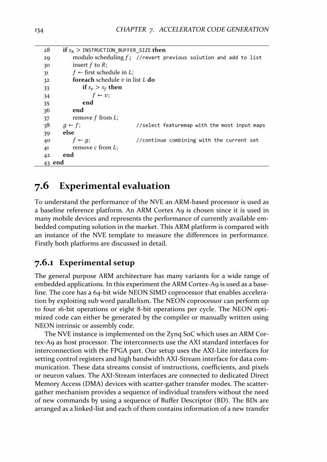
134 CHAPTER 7. ACCELERATOR CODE GENERATION
28 if 𝑠ℎ > INSTRUCTION_BUFFER_SIZE then 29 modulo scheduling 𝑓; //revert previous solution and add to list 30 insert 𝑓 to 𝑅; 31 𝑓 ← first schedule in 𝐿; 32 foreach schedule 𝑣 in list 𝐿 do 33 if 𝑠𝑣 > 𝑠𝑓 then
34 𝑓 ← 𝑣; 35 end 36 end 37 remove 𝑓 from 𝐿; 38 𝑔 ← 𝑓; //select featuremap with the most input maps 39 else 40 𝑓 ← 𝑔; //continue combining with the current set 41 remove 𝑐 from 𝐿; 42 end 43 end
7.6 Experimental evaluation
To understand the performance of the NVE an ARM-based processor is used as a baseline reference platform. An ARM Cortex A9 is chosen since it is used in many mobile devices and represents the performance of currently available em-bedded computing solution in the market. This ARM platform is compared with an instance of the NVE template to measure the differences in performance. Firstly both platforms are discussed in detail.
7.6.1 Experimental setup
The general purpose ARM architecture has many variants for a wide range of embedded applications. In this experiment the ARM Cortex-A9 is used as a base-line. The core has a 64-bit wide NEON SIMD coprocessor that enables accelera-tion by exploiting sub word parallelism. The NEON coprocessor can perform up to four 16-bit operations or eight 8-bit operations per cycle. The NEON opti-mized code can either be generated by the compiler or manually written using NEON intrinsic or assembly code.
The NVE instance is implemented on the Zynq SoC which uses an ARM Cor-tex-A9 as host processor. The interconnects use the AXI standard interfaces for interconnection with the FPGA part. Our setup uses the AXI-Lite interfaces for setting control registers and high bandwidth AXI-Stream interface for data com-munication. These data streams consist of instructions, coefficients, and pixels or neuron values. The AXI-Stream interfaces are connected to dedicated Direct Memory Access (DMA) devices with scatter-gather transfer modes. The scatter-gather mechanism provides a sequence of individual transfers without the need of new commands by using a sequence of Buffer Descriptor (BD). The BDs are arranged as a linked-list and each of them contains information of a new transfer

7.6. EXPERIMENTAL EVALUATION 135
such as starting address, size, and pointer to the next BD. The ARM core places the BDs in memory after which it initiates the execution sequence. Then the DMAs automatically fill the instruction memory, and continue with pixel pro-cessing. Our code correctness is verified by executing generated programs for our face detection and speed sign detection workloads (see Chapter 3).
7.6.2 Performance metrics
Our definition of code quality is the number of computations (effective MACCs) per VLIW instruction. This represents only effective workload, but note that there are many load/store ops., and data reorder ops. that are neglected by this definition. Low quality code has a low MACC unit utilization due to NOP slots in the pipeline or loop overhead (additional prolog/epilog code to start and finish a loop). Additionally, the amount of external data transfer is important. Firstly, it can stall the pipeline if DMAs cannot keep up with the accelerator, and sec-ondly it is often bad for energy consumption.
7.6.3 Performance analysis
CONVE generated code quality is evaluated by comparison against manual cod-ing by architecture experts. These experts spent days to write and optimize a complete ConvNet assembly program which is generated in a few seconds by our compiler. Figure 7.10 summarizes the performance on our benchmarks for dif-ferent optimization flows. For example, the first graph gives the performance of manual mapping, compared to the second (CONVE without optimization) the
0
2
4
6
8
10
12
14
16
L1 L2 L3 L4 L1 L2 L3 L4
Face Detection Speed Sign Detection 3x3
MA
CC
/ in
stru
ctio
n
Manual Automatic Automatic + Coeff. Packing Automatic + Coeff. Packing + Modulo Sched. Automatic + Coeff. Packing + Modulo Sched. + Combining
Figure 7.10: HW utilization comparison of manually written programs versus multiple performance settings of the automatically generated programs.

136 CHAPTER 7. ACCELERATOR CODE GENERATION
manual mapping achieves a 7 up to 28% better MACC unit utilization. This in-dicates that the default CONVE flow is already quite competitive to a fine-tuned manual mapping.
The set of bars on the left hand side shows performance on the educational example of a 3x3 convolution. Both steady-state schedules with 10 instructions manual and 14 automatic is relatively short, therefore the relative performance difference is large. In a dense workload like layer 3 of our speed sign application the difference is relatively small. Both steady-state schedules contain over 200 instructions. This example shows that workloads will behave different and it is not always obvious why code under-performs. For very long schedules the effect of missing modulo scheduling is relatively small, since the borders of a schedule represent a minor portion. On the other hand, for short schedules like in our 3x3 convolution this effect is very dominant.
The first optimization performs resource conflict resolving through coeffi-cient layout optimization, which reduces the number of NOP slots. On average coefficient repacking improves performance by 2%. For layer 3 of the speed sign detection workload the schedule compresses enough to beat the manual expert. This is an example where the schedule was too complicated for our manual ex-pert programmer, hence he could not find all optimizations. For some short schedules like 3x3 convolution the removal of NOP slots does not reduce the schedule length, which is due to the necessary stores in the scratchpad memory.
The second optimization reduces under-utilization between iterations of the schedule by modulo scheduling. Modulo scheduling on average gives an addi-tional performance improvement of 7%. With modulo scheduling most bench-mark layers perform very close to the manual implementation. For the very dense ConvNet layers like layer 3 the performance is very important since they represent the major part of application workload. It is clear that for these dense layers the performance is close to the accelerator peak performance of 16 MACCs per instruction. For the other layers the performance lacks behind, which is of-ten caused due to communication bandwidth limitations on the local scratchpad ports. Layer 1 and 2 of both applications contain a 2x2 pooling which increases the data volume for 16 parallel convolution results. In layer 4 there is even less register reuse due to 1x1 convolution operations. Both configurations stress the scratchpad memory bandwidth.
The final optimization under evaluation is featuremap combining which in-creases data locality. For some layers the number of scratchpad store operations are reduced which gives a performance increase, see Figure 7.10. More important is the data communication reduction with external memory. Figure 7.11, reveals that featuremap combining is sometimes needed to perform on-par with the manual experts. Due to our efficient inter-tile execution patterns data-reuse in convolution windows and over input featuremaps is already very well utilized. Mostly the sparsely connected layers such as layer 1 and 2 benefit from this op-timization. Note the large communication reductions on the logarithmic scale. In very dense layers the instruction loop buffer with only 512 entries prevents

7.7. CONCLUSIONS 137
combining feature maps. To enable combining for these layers a larger instruc-tion buffer and a larger scratchpad memory are required.
Combining all optimizations improves MACC unit utilization up to 16.5%. However for some layers like output layer 4 of the benchmarks CONVE gener-ated schedules perform 20% worse than the manual code. In this case the man-ual programmer uses half vectors (8 MACC operations), which is not yet available in CONVE. For the evaluated NVE instance the half vectors reduce load pressure from scratchpad port A. Remember that layer 4 is only a small portion of the total workload. The performance of the complete benchmark applications (all layers) is better for the CONVE generated code. In conclusion for very specific workloads (layer 4) the manual programmer is the better one, but for large com-plicated workloads CONVE performs better, see layer 3. In addition, our fea-turemap combining step improves data locality at the cost of more complicated schedules. A manual programmer faces a huge challenge when he has to imple-ment such combinations. It is simply difficult to overlook the huge set of sched-ule combinations and match those with the many platform constraints.
7.7 Conclusions
Dedicated hardware accelerators for Convolutional Networks (ConvNets) have substantially improved the computational efficiency of this challenging algo-rithm. One of the remaining bottlenecks for broad usage of such accelerators is the large complexity involved when programming such accelerators. For many of the proposed accelerators this problem is simply ignored, as a result these
1
10
100
1000
L1 L2 L3 L4 L1 L2 L3 L4
Face Detection Speed Sign Detection 3x3
Dat
a Tr
ansf
ers
(10
3w
ord
s o
f 6
4 b
it)
Manual Automatic Automatic + Coeff. Packing Automatic + Coeff. Packing + Modulo Sched. Automatic + Coeff. Packing + Modulo Sched. + Combining
Figure 7.11: Data transfer comparison of manually written programs versus different con-figurations of automatically generated programs.
138 CHAPTER 7. ACCELERATOR CODE GENERATION
accelerators are often not used in embedded platforms due to their huge map-ping complexity.
We demonstrated with our new COmpiler for Neuro Vector Engines (CONVE) that optimized accelerator code for VLIW based vector accelerators can be generated from high-level .JSON ConvNet descriptions. This technique is very generic and straight forward such that it can be applied to different in-stances of the NVE template. By using advanced code optimization with Modulo Scheduling and data layout optimization CONVE generates codes that achieves hardware utilization levels on-par with code manually optimized by architecture experts. Due to techniques like inter-tile optimization and feature-map combin-ing our generated code has better data locality, which reduces the challenging data transfer requirements.
The introduction of the CONVE flow enables users to abstract from the NVE accelerator architecture and only specify a ConvNet and choose an instance of the NVE Template. This abstraction reduces the programming workload for ConvNet vision application development from days to minutes. The removal of this last productivity bottleneck enables the adoption of ConvNets in the next-generation mobile and wearable devices. This step will bring 'intelligent' features like real-time machine vision and speech translation to our portable compan-ions.

139
8.
CONCLUSIONS AND FUTURE WORK
This chapter concludes the thesis. It is subdivided in two main sections. The first summarizes the conclusions of the individual chapters and reflects how these address the issues identified in the problem statement of Chap-ter 1. The second section presents some open issues that still remain to be solved, as well as, ideas that are not fully worked out and remain as future work.
8.1 Conclusions
Deep Learning and Convolutional Networks (ConvNets) have become increas-ingly popular as pattern recognition methods to solve complicated problems in many different domains. These machine learning techniques have set many new accuracy records and have shown super human performance on various tasks. However, for consumer applications in the mobile or wearable domain these im-pressive classifier models are not often used. The huge number of model param-eters and the challenging compute workload make it difficult to use these nets on an ultra-low power platform. The general purpose CPUs and GPUs do not fit the power requirements and embedded processors do not deliver the required performance. The use of these techniques in embedded platforms is key to de-velop save autonomous driving solutions. Or it should give drones the intelli-gence to automatically navigate and deliver packages that are ordered remotely. In continuously operating or so called “always on” wearable companion devices, it could help us in daily tasks. For these reasons industry and academia have started to investigate different techniques to improve the energy efficiency of ConvNets. This has led to various results on high-level optimizations, dedicated function accelerators, and compilation frameworks for deployment.
The problem statement (Chapter 1.4) defines the number of required com-pute operations as one of the key quantitative properties that influences the en-ergy efficiency. Chapter 4 of this thesis addresses the huge computational
CHAPTER

140 CHAPTER 8. CONCLUSIONS AND FUTURE WORK
workload in ConvNets by an algorithmic transformation that merges Convolu-tion and Averaging Pooling layers. Our technique can be used on trained net-works with average pooling layers without sacrificing accuracy. On the other hand it can also be used to train new nets with merged layers, which enables approximation and replacement of nets having max pooling layers. Real bench-mark applications demonstrate 65% to 83% workload reduction, without reduc-ing accuracy. The impact of MACC workload reduction on compute performance is measured with a CPU and GPU platform mapping. Compared to the original convolution and subsample part the CPU mapping is 2.7 times faster where the GPU mapping improves 2.5 times. An efficiency improvement of 2.5-2.7 times is a first step towards mapping on power constrained platforms. The important part is that this optimization can be combined with other optimiza-tions to achieve a much more aggressive efficiency improvement.
Another important other efficiency problems is data movement. The thesis problem statement defines the number of external memory transfers as a quan-titative metric for data movement efficiency. Nowadays, data movement is re-sponsible for a large portion of the consumed energy in compute platforms. Inter-tile data reuse optimization is a new tiling or blocking technique that con-siderably improves data reuse in nested loop accelerators. Before this work ac-celerators could exploit the data overlap between successive tiles, but not automatically shape the tiles to maximize this overlap. With real benchmarks we show that optimizing the tile shape for inter-tile reuse can further reduce external memory accesses up to 52% compared to an already aggressively opti-mized schedule. To exploit maximum inter-tile overlap we developed an analyt-ical data reuse model that quickly gives the number of external accesses and the required buffer size to fit this schedule into a local scratchpad. With our model-based search approach we obtain the best schedules in mere seconds. These best schedules are evaluated with real FPGA mappings done by the Xilinx Vivado HLS tools. This resulted in a locality optimized design workflow that eases the map-ping of ConvNets to dedicated hardware accelerators.
Dedicated function accelerators in FPGAs are a flexible alternative for CPUs and GPUs. To improve the energy-efficiency even further we propose the Neuro Vector Engine (NVE), a flexible accelerator template for ASIC implementation. The NVE performs extremely efficient SIMD operations on vector words. In ad-dition, it has flexible VLIW-type control such that it can use layer merging and inter-tile reuse optimizations. This combines the optimizations from earlier chapters into an efficient accelerator template. Synthesis of a good performing instance of the template with a 40nm low power TSMC library demonstrated that the NVE is a very small design, requiring only 0.259 mm2. On our real world speed sign recognition benchmark and face detection application our 1 Ghz in-stance achieves 30.2 GOp/s. This is 20 times faster than our NEON optimized mappings on an ARM-A9 Core. In addition, it is benchmarked against CUDA optimized mappings for an NVIDIA TK1 embedded GPU. Depending on the layer configurations the NVE is 1.2 to 2.6 times faster than the GPU. Considering the ultra-low power consumption of NVE (only 54 mW), this is a very impressive
8.2. FUTURE WORK 141
result. Especially the high degree of flexibility makes that our NVE has a high utilization which is important for efficiency. Many other accelerators are too dedicated to the convolution operation. As a result, they require more data movement, or have a low utilization during several stages of the algorithm; both reduce energy efficiency substantially.
This thesis has shown that dedicated accelerators can bridge the energy effi-ciency gap for ConvNets. However, the programmability of many accelerators can be improved a lot from both an architectural and a compiler perspective. The thesis problem statement defines the utilization level that a normal pro-grammer can achieve when mapping different network workloads as a quantita-tive metric for flexibility, which again results into efficiency. Our work proposes a flexible VLIW instruction format for the NVE to obtain a very programmable architecture. In addition, the compiler part opens opportunities to improve ap-plication portability and designer productivity by abstracting away from target specific assembly languages. Our COmpiler for Neuro Vector Engines (CONVE) addresses the portability and productivity problems. By using an abstract .JSON network description the programmer does not have to think of architectural de-tails. Also the application fine tuning is handled by the CONVE framework. Ad-vanced code optimizations such as, modulo scheduling, and feature map combining ensure that an expert level of optimization is achieved automatically.
Although this thesis focused on a broad range of techniques to improve the computational efficiency of ConvNets, it is also applicable to a much broader application domain. Other image/video processing pipelines, such as Motion Es-timation for video coding can benefit from the proposed contributions. Algo-rithms that require several Linear Algebra operations can be made much more efficient with the contributions of this thesis. In Chapter 5 we presented detailed evaluations of the effect of inter-tile reuse optimization for such applications. In addition the NVE is basically a vector processor that can accelerate these and many other workloads for the embedded domain. This also holds for the quickly developing field of Deep Learning. New network architectures that contain for instance residual nodes or recurrent nodes can benefit a lot from the ideas on inter-tile reuse and the NVE with the CONVE framework.
8.2 Future work
This thesis is written in a time where Deep Learning based algorithms became very popular. Nowadays many research groups are studying the efficiency prob-lems in deep learning. Keeping up with the state-of-the-art was one of the major challenges for this work. This section will discuss limitations of this work with regard to new deep learning techniques. In addition, to a changing field with new contributions we encountered several opportunities for improvement of the various efficiency optimization techniques. Some of these opportunities deserve to be mentioned as possible extensions of the presented work.

142 CHAPTER 8. CONCLUSIONS AND FUTURE WORK
Network compression for further computational workload reduction: Very re-cent works on workload reduction have further reduced the computational re-quirements [60,120]. For instance they perform advanced network pruning techniques that remove unnecessary parts in deep networks. This often reduces the required computational workload, but it makes networks less regular. Our layer merging technique and fixed point accuracy exploration from Chapter 4 had a similar goal. However, our early work from 2011 did not go as far as these new solutions. Still our work is very valuable next to other works. For example the Deep Compression work [60] focuses on reducing the weight set. The huge amount of intermediate neuron data per layer should still be communicated to larger memories. Their work could be further improved by merging layers like we did. This will reduce the intermediate data communication significantly. An-other aspect is the regularity of the networks. Our reduction maintains a regular network structure where these newer techniques create very irregular and sparse structures. For these compute workloads it is difficult to achieve a high utiliza-tion. Future work into more advanced architectures is necessary to cope effi-ciently with very irregular compute workloads. Alternatively, we need different network compression techniques that enforce regular network structure to ex-ploit existing computer architecture techniques such, as sub word parallelism by SIMD, and spatial locality by wide cache lines.
Aggressive data locality optimization by layer fusion and re-computation: Our work on inter-tile reuse optimization (Chapter 5) is an important technique to improve the data locality for deep ConvNets. However, we did not address the depth of the networks. Inter-tile optimizations are performed on single or a merged layer. New recent works exploit the data reuse over successive layers [2]. The difficulty in fusing layers is the growing set of data dependencies per layer. Before fusing two layers a portion of the fist layer must be computed, next this portion is consumed by the second layer. This producer consumer relation and the fact that a larger portion from an early layer is required to compute a small portion of a later layer make it difficult to implement fusion efficiently. Also the work in [2] is challenged with these dependencies. They use sliding window tiles that contain a few fused layers. For these fused tiles a lot of local buffer space is required to meet the inter layer dependencies. We developed an early technique to fuse layers as addition to the inter-tile work. It is quite easy to interleave suc-cessive tile strips from succeeding layers. Our new method does even take re-computation of intermediate results into account to reduce the number of de-pendency constraints. As a result, an additional external traffic reduction of 1.5 to 2 times is demonstrated upon the best schedules of our inter-tile work. This work is presented on the NeuroArch workshop at ISCA 2014 [102]. At the time of writing this thesis we are working out the mathematical details of this improved data locality optimization technique.
Improving the NVE template: During our work on the NVE accelerator tem-plate we identified opportunities for further improvement. The NVE aims at the ultra-low power embedded SoC domain. Therefore, the energy efficiency is very

8.2. FUTURE WORK 143
high at an effective compute throughput (in multiply and accumulate opera-tions) in the range of 30 Gop/s. A silicon efficiency of 115 Gops/mm2 and an en-ergy efficiency of 559 Gops/W is demonstrated. Note that in addition to the 30 Gop/s of effective neuron operations a substantial amount of data re-order and address computation is performed by the dedicated function units. Scaling up the effective performance beyond 300 Gop/s is rather difficult. Wider vector pro-cessing gives a performance increase but, it reduces the vector MACC unit utili-zation and thereby the energy efficiency. To increase performance further a multiprocessor configuration should be developed. Since data sharing between processing nodes is key the multiprocessor design should have a flexible com-munication structure.
Memory reordering units for the NVE: The NVE benefits from excellent data locality in the computations due to inter-tile reuse optimization. This works very well if incoming and outgoing data streams are controlled by flexible Direct Memory Access (DMA) controllers. In a report [152] we show the first efforts towards flexible DMA devices. These can offer high bandwidth and flexibility. Further improvements on dedicated DMAs and the memory subsystem are im-portant for accelerator developments.
More efficient ConvNet operations: As demonstrated in this thesis the com-putational workload in a ConvNet is dominated by MACC operations. To im-prove the efficiency at the operator level we could further improve these MACC operations. In a short study we looked into Carry Save Multiply Accumulates. It requires that the accumulator uses numbers in its carry save format. This signif-icantly reduces the complexity of multiplications and the accumulations. Only after the last accumulation the independent sum and carry part should be com-bined with a more costly conventional adder. This technique could be further developed and used as a compute element in the NVE template to increase effi-ciency.
Compute architecture for irregular ConvNets: With the introduction of XNOR-net [120] and network compression techniques [60] their workload has become irregular. These new techniques have e.g. introduced the requirement to perform sparse matrix operations efficiently. However, from a compute per-spective this opens new challenges for computational efficiency. The work in [59] is one of the first accelerator architectures that focusses on the irregular operations for compressed networks. These new works design advanced circuits to perform network operators very efficiently. However, these irregular work-loads require a well-tuned ISA to achieve flexibility and efficiency. Maybe the ISA is even more important since the program control becomes more compli-cated. In addition, good compilers such as our CONVE framework are key to achieve good hardware utilization on such sparse network accelerators. Future work in these domains are important to further increase ConvNet efficiency.

144
BIBLIOGRAPHY
[1] C. Alias, A. Darte, and A. Plesco, "Optimizing Remote Accesses for Offloaded Kernels: Applications to high-level synthesis for fpga," in Proceedings of the Conference on Design, Automation and Test in Europe (DATE '13), 2013, pp. 575-580.
[2] M. Alwani, H. Chen, M. Ferdman, and P. Milder, "Fused-Layer CNN accelerators," in 49th Annual IEEE/ACM International Symposium on Microarchitecture (MICRO), 2016, pp. 1-12.
[3] B. Bayer, "Color imaging array," US Patent 3,971,065, 1976.
[4] H. Bay, T. Tuytelaars, and L. van Gool, "Surf: Speeded up robust features," in Computer vision - ECCV, 2006, pp. 404-417.
[5] Y. Bengio, "Practical recommendations for gradient-based training of deep architectures," in Neural Networks: Tricks of the Trade, K.-R. Müller, G. Montavon, and G.B. Orr, Eds.: Springer, 2013, ch. 19.
[6] K. Beyls and E.H. D'Hollander, "Refactoring for data locality," Computer, vol. 42, no. 2, pp. 62-71, 2009.
[7] N. Binkert et al., "The gem5 simulator," SIGARCH Computer Architecture News, vol. 39, no. 2, pp. 1-7, 2011.
[8] U. Bondhugula et al., "Automatic Transformations for Communication-minimized Parallelization and Locality Optimization in the Polyhedral Model," in Proceedings of the Joint European Conferences on Theory and Practice of Software 17th International Conference on Compiler Construction , 2008, pp. 132-146.
[9] U. Bondhugula, A. Hartono, J. Ramanujam, and P. Sadayappan, "A practical and fully automatic polyhedral program optimization system," in Proceedings of the 29th ACM SIGPLAN Conference on Programming Language Design and Implementation (PLDI), 2008, pp. 101-113.
[10] S. Borkar and A.A. Chien, "The future of microprocessors," Communications of the ACM, vol. 54, no. 5, pp. 67-77, 2011.
[11] L. Bottou, "Large-scale machine learning with stochastic gradient descent," in In Proceedings of COMPSTAT, 2010, pp. 177-186.
145
[12] L. Bottou, "Stochastic gradient descent tricks," in Neural Networks: Tricks of the Trade.: Springer, 2012, ch. 18, pp. 421-436.
[13] L. Bottou et al., "Comparison of classifier methods: a case study in handwritten digit recognition," in Proceedings of the 12th International Conference on Pattern Recognition and Neural Network, 1994, pp. 77-82.
[14] F. Catthoor et al., Data access and storgage management for embedded programmable processors.: Springer Science & Business Media, 2013.
[15] L. Cavigelli et al., "Origami: A convolutional network accelerator," in 25th edition of the ACM/IEEE Great Lakes Symposium on VLSI (GLS-VLSI), 2015, pp. 199-204.
[16] Srimat Chakradhar, Murugan Sankaradas, Venkata Jakkula, and Srihari Cadambi, "A dynamically configurable coprocessor for convolutional neural networks," in Proceedings of the 37th annual international Symposium on Computer Architecture, 2010.
[17] K. Chandrasekar, B. Akesson, and K. Goossens, "Improved Power Modeling of DDR SDRAMs," in Euromicro Conference on Digital System Design (DSD), 2011, pp. 99-108.
[18] K. Chellapilla, S. Puri, and P. Simard, "High performance convolutional neural networks for document processing," in 10th International Workshop on Frontiers in Handwriting Recognition, 2006.
[19] T.-C. Chen et al., "Analysis and architecture desing of an hdtv 720p 30 frames/s h264/avc encoder," IEEE Transactions on Circuits and Systems for Video Technology, pp. 16:673-688, 2006.
[20] T. Chen et al., "DianNao: a small-footprint high-throughput accelerator for ubiquitous machine-learning," in Proceedings of the 19th international conference on Architectural support for programming languages and operating systems, 2014, pp. 269--284.
[21] Y. Chen, J. Emer, and V. Sze, "Eyeriss: A Spatial Architecture for Energy-efficient Dataflow for Convolutional Neural Networks," in Proceedings of the 43rd International Symposium on Computer Architecture (ISCA), Seoul, Republic of Korea, 2016, pp. 367-379.
[22] Y. Chen, T. Krishna, J. Emer, and V. Sze, "Eyeriss: An energy-efficient reconfigurable accelerator for deep convolutional neural networks," in IEEE International Solid-State Circuits Conference (ISSCC), 2016, pp. 262-263.
[23] Y. Chen, Z. Lin, X. Zhao, G. Wang, and Y. Gu, "Deep Learning-Based Classification of Hyperspectral Data," IEEE Journal of Sleceted Topics in Applied Earth Observations and Remote Sensing, vol. 7, no. 6, pp. 2094-2107, June 2014.
[24] W. Chen, J.T. Wilson, S. Tyree, K.Q. Weinberger, and Y. Chen, "Compressing neural networks with the hashing trick," in Proceedings of

146 BIBLIOGRAPHY
the 32nd International Conference on Machine Learning, 2015, pp. 2285-2294.
[25] D. Ciresan, A. Giusti, L.M. Gambardella, and J. Schmidhuber, "Deep Neural Networks Segment Neuronal Membranes in Electron Microscopy Images," Advances in Neural Information Processing Systems 25, pp. 2843-2851, 2012.
[26] D.C. Ciresan, A. Giusti, L.M. Gambardella, and J. Schmidhuber, "Mitosis detection in breast cancer histology images with deep neural networks," in Medical Image Computing and Computer-Assisted Intervention-MICCAI, 2013, pp. 411-418.
[27] D.C. Ciresan, U. Meier, L.M. Gambardella, and J. Schmidhuber, "Deep, big, simple neural nets for handwritten digit recognition," Neural Computation, vol. 22, no. 12, pp. 3207-3220, 2010.
[28] D.C. Ciresan, U. Meier, J. Masci, J.M. Gambardella, and J. Schmidhuber, "Flexible, high performance convolutional neural networks for image classification," in IJCAI Proceedings-International Joint Conference on Aritficial Intelligence, 2011, pp. 1237-1242.
[29] D.C. Ciresan, U. Meier, J. Masci, and J. Schmidhuber, "A committee of neural networks for traffic sign classification," in IJCNN International Conference on Neural Networks, 2011, pp. 1918-1921.
[30] D. Cireşan, U. Meier, J. Masci, and J. Schmidhuber, "Multi-column deep neural network for traffic sign classification," Neural Networks, vol. 32, pp. 333-338, 2012.
[31] D.C. Ciresan, U. Meier, and J. Schmidhuber, "Multi-column deep neural networks for image classification," in IEEE Conference on Computer Vision and Pattern Recognition (CVPR), 2012, pp. 3642-3649.
[32] A. Coates, B. Huval, T. Wang, D.J. Wu, and A.Y. Ng, "Deep learning with COTS HPC systems," in Proceedings of the 30th international conference on machine learning, 2013, pp. 1337-1345.
[33] L. Codrescu et al., "Hexagon DSP: an Architecture Optimized for Mobile Multimedia and Communications," IEEE Micro, vol. 34, no. 2, pp. 34-43, March 2014.
[34] R. Collobert, K. Kavukcuoglu, and C. Farabet, "Torch7: A matlab-like environment for machine learning," in BigLearn, NIPS Workshop, 2011.
[35] F. Comaschi, S. Stuijk, T. Basten, and H. Corporaal, "RASW: a run-time adaptive sliding window to improve viola-jones object detection," in Proceedings of 7th International Conference on Distributed Smart Cameras ICDSC, 2013, pp. 1-6.
[36] J. Cong and B. Xiao, "Minimizing computation in convolutional neural networks," in International Conference on Aritficial Neural Networks, 2014, pp. 281-290.

147
[37] F. Conti and L. Benini, "A Ultra-Low-Energy Convolution Engine for Fast Brain-Inspired Vision in Multicore Clusters," in Proceedings of the Desing, Automation & Test in Europe Conference & Exhibition, 2015, pp. 683-688.
[38] N. Dalal and B. Triggs, "Histograms of oriented gradients for human detection," in IEEE Computer Society Conference on Computer Vision and Pattern Recognition CVPR, 2005, pp. 886-893.
[39] N. Dalal and B. Triggs, "Histograms of Oriented Gradients for Human Detection," in Proceedings of the IEEE Computer Society Conference on Computer Vision and Pattern Recogniton CVPR, 2005, pp. 886-893.
[40] A. Darte and A. Isoard, "Parametric Tiling with Inter-Tile Data Reuse," in In 4th International Workshop on Polyhedral Compilation Techniques (IMPACT'14), 2014.
[41] G. De Haan, P.W. Biezen, H. Huijgen, and O.A. Ojo, "True-motion estimation with 3-D recursive search block matching," IEEE Transactions on Crircuits and Systems for Video Technology, vol. 3, no. 5, pp. 368-379, 1993.
[42] R.H. Dennard, J. Cai, and A. Kumar, "A perspective on today's scaling challenges and possible future directions," Solid-State Electronics, vol. 51, no. 4, pp. 518-525, 2007.
[43] G. Desoli et al., "A 2.9 Tops/w deep convolutional neural network soc in fd-soi 28nm for intelligent embedded systems," in IEEE International Solid-State Circuits Conference, 2017, pp. 238-239.
[44] C. Ding and Y. Zhong, "Predicting Whole-program Locality Through Reuse Distance Analysis," in PLDI '03, 2003, pp. 245-257.
[45] C. Ding and Y. Zhong, "Reuse Distance Analysis," University of Rochester, 2001.
[46] Z. Du et al., "ShiDianNao: Shifting vision processing closer to the sensor," in Proceedings of the 42nd Annual International Symposium on Computer Architecture ISCA, Portland, Oregon, 2015, pp. 92-104.
[47] D. Erhan et al., "Why does unsupervised pre-training help deep learing?," Journal of Machine Learning Research, pp. 625-660, 2010.
[48] H. Esmaeilzadeh, E. Blem, R. St. Amant, K Sankaralingam, and D Burger, "Dark Silicon and the End of Multicore Scaling," in 38th Annual International Symposium onComputer Architecture (ISCA), 2011, pp. 365-376.
[49] C. Farabet, C. Couprie, L. Najman, and Y. LeCun, "Learning hierarchical features for scene labeling," Pattern Analysis and Machine Intelligence, IEEE Transactions on, vol. 35, pp. 1915-1929, 2013.
[50] C. Farabet et al., "Neuflow: A runtime reconfigurable dataflow processor for vision," in IEEE Computer Society Conference on Computer Vision and Pattern Recognition Workshops (CVPRW), 2011, pp. 109-116.
148 BIBLIOGRAPHY
[51] C. Farabet, C. Poulet, J. Han, and Y. LeCun, "An FPGA-based processor for convolutional networks," in International Conference on Field Programmable Logic and Applications FPL , 2009, pp. 32-37.
[52] J.A. Fisher, P. Faraboschi, and C. Young, Embedded Computing: A VLIW Approach to Architecture, Compilers and Tools.: Morgan Kaufmann, 2012.
[53] C Garcia and M Delakis, "Convolutional face finder: a neural architecture for fast and robust face detection," IEEE Transaction on Pattern Analysis and Machine Intelligence, vol. 26, pp. 1408-1423, 2004.
[54] R. Girshick, "Fast R-CNN," in Proceedings of the IEEE International Conference on Computer Vision (ICCV), 2015.
[55] R. Girshick, J. Donahue, T. Darrell, and J. Malik, "Rich feature hierarchies for accurate object detection and semantic segmentation," in Proceedings of the IEEE conference on computer vision and pattern recognition, 2014, pp. 580-587.
[56] X. Glorot, A. Bordes, and Y. Bengio, "Deep Sparse Rectifier Neural Networks," in 14th International Conference on Artificial Intelligence and Statistics, 2011, pp. 315-323.
[57] R.E. Gonzales, "Xtensa: a configurable and extensible processor," in IEEE Micro, 2000, pp. 60-70.
[58] R. Hameed et al., "Understanding sources of inefficiency in general-purpose chips," ACM SIGARCH Computer Architecture News, vol. 38, no. 3, pp. 37-47, 2010.
[59] S. Han et al., "EIE: Efficient Inference Engine on Compressed Deep Neural Networks," in Proceedings of the 43rd International Symposium on Computer Architecture (ISCA), 2016, pp. 243-254.
[60] S. Han, H. Mao, and W.J. Dally, "Deep Compression: Compressing Deep Neural Networks with Pruning, Trained Quantization and Huffman Coding," in International Conference on Learning Representations (ICLR), 2016.
[61] S.O. Haykin, Neural Networks and Learning Machines, 3rd ed.: Prentice Hall, 2008.
[62] K. He, X. Zhang, S. Ren, and J. Sun, "Deep Residual Learning for Image Recognition," arXiv preprint arXiv: 1512.03385, 2015.
[63] K. He, X. Zhang, S. Ren, and J. Sun, "Delving deep into rectifiers: Surpassing human-level performance on ImageNet classification," in The IEEE International Conference on Computer Vision (ICCV), 2015, pp. 1026-1034.
[64] G.E. Hinton, "Connectionist learing procedures," Artificial intelligence, vol. 40, no. 1, pp. 185-234, 1989.
[65] G.E. Hinton, "Connectionist learning procedures," Artificial intelligence, vol. 40, no. 1, pp. 185-234, 1989.

149
[66] G. Hinton et al., "Deep Neural Networks for Acoustic Modeling in Speech Recognition: The Shared Views of Four Research Groups," Signal Processing Magazine, IEEE, vol. 29, pp. 82-97, 2012.
[67] G.E. Hinton, S. Osindero, and Y.W. Teh, "A fast learning algorithm for deep belief nets," Neural computation, vol. 18, no. 7, pp. 1527-1554, 2006.
[68] G.E. Hinton and R.R. Salakhutdinov, "Reducing the dimensionality of data with neural networks," Science, vol. 313, no. 5786, pp. 504-507, 2006.
[69] G.E. Hinton, N. Srivastava, A. Krizhevsky, I. Sutskever, and R. Salakhutdinov, "Improving neural networks by preventing co-adaptation of feature detectors," Technical Report, arXiv: 1207.0580 2012.
[70] J.L. Holi and J.N. Hwang, "Finite precision error analysis of neural network hardware implementations," IEEE Transactions on Computers, vol. 42, no. 3, pp. 281-290, 1993.
[71] G. Huang, M. Mattar, H. Lee, and E.G. Learned-Miller, "Learning to align from scratch," In Advances in Neural Information Processing Systems, pp. 764-772, 2012.
[72] Intel. ARK Processor Database. [Online]. http://ark.intel.com/
[73] S. Ioffe and C. Szegedy, "Batch normalization: Accelerating deep network training by reducing internal covariate shift," in ICML, 2015.
[74] I. Issenin, E. Brockmeyer, M. Miranda, and N. Dutt, "DRDU: A Data Reuse Analysis Technique for Efficient Scratch-pad Memory Management," ACM Trans. Des. Autom. Electron. Syst., vol. 12, no. 2, 2007.
[75] M. Jaderberg, A. Vedaldi, and A. Zisserman, "Speeding up convolutional neural networks with low rank expansions," arXiv preprint, arXiv:1405.3866 2014.
[76] Y. Jia et al., "Caffe: Convolutional Architecture for Fast Feature Embedding," in Proceedings of the 22nd ACM International Conference on Multimedia, Orlando, Florida, USA, 2014, pp. 675-678.
[77] N.P. Jouppi et al., "In-datacenter performance analysis of a tensor processing unit," in Proceedings of the 44th Annual International Symposium on Computer Architecture (ISCA), 2017, pp. 1-12.
[78] D. Kline and V. Berardi, "Revisting squared-error and cross-entropy functions for training neural networks classifiers," Neural Computing & Applications, vol. 14, no. 4, pp. 310-318, 2005.
[79] A. Krizhevsky, S. Ilya, and G.E. Hinton, "ImageNet Classification with Deep Convolutional Neural Networks 25," Advances in Neural Information Processing Systems, pp. 1097-1105, 2012.
[80] M. Lam, "Software pipelining: an effective scheduling technique for VLIW machines," in Proceedings of the ACM SIGPLAN conference on Programming language design and implementation (PLDI), 1988, pp. 318-328.
150 BIBLIOGRAPHY
[81] A. Lavin and S. Gray, "Fast algorithms for convolutional neural networks," arXiv preprint, preprint arXiv: 1509.09308, 2015.
[82] Y. LeCun et al., "Backpropagation Applied to Handwritten Zip Code Recogonition," Neural Computation, vol. 1, no. 4, pp. 541-551, 1989.
[83] Y. LeCun et al., "Handwritten Digit Recognition with a Back-propagation Network," Advances in Neural Information Processing Systems NIPS 2, pp. 396-404, 1990.
[84] Y. Lecun, L. Bottou, Y. Bengio, and P. Haffner, "Gradient-based learning applied to document recognition," Proceedings of the IEEE, vol. 86, no. 11, pp. 2278-2324, Nov 1998.
[85] Y. LeCun, F.J. Huang, and L. Bottou, "Learning methods for generic object recognition with invaricance to pose and lighting," in Proceedings of the Computer Society Converencde on Computer Vision and Pattern Recognition CVPR, 2004, pp. 97-104.
[86] Y. LeCun, U. Muller, J. Ben, E. Cosatto, and B. Flepp, "Off-road obstacle avoidance through end-to-end learning," Advances in Neural Information Processing Systems, pp. 739-746, 2005.
[87] Q.V. Le et al., "Building high-level features using large scale unsupervised learing," in IEEE International Conference on Acoustics, Speech and Signal Processing (ICASSP), 2013, pp. 8595-8598.
[88] S. Li et al., "Mcpat: An integrated power, area, and timing modeling framework for multicore and manycore architectures," in Proccedings of the 42nd Annual IEEE/ACM International Symposium on Microarchitecture, 2009, pp. 469-480.
[89] W. Liu et al., "SSD: Single Shot MultiBox Detector," in European conference on computer vision (ECCV), 2016.
[90] Q. Liu, G.A. Constantinides, K. Masselos, and P.Y.K. Cheung, "Combining Data Reuse With Data-Level Parallelization for FPGA-Targeted Hardware Compilation: A Geometric Programming Framework," in IEEE Transactions on Computer-Aided Design of Integrated Circuits and Systems, vol. 28, no. 3, pp. 305-315, 2009.
[91] D.G. Lowe, "Object recognition from local scale-invariant features," in Proceedings of the 7th IEEE International Coference on Computer Vision, 1999, pp. 1150-157.
[92] R. Malvar, L. He, and R. Cutler, "High-Quality Linear Interpolation for Demosaicing of Bayer-Patterned Color Images," in IEEE International Conference of Acoustic, Speech and Signal Processing, 2004.
[93] J. Ma, R.P. Sheridan, A. Liaw, G.E. Dahl, and V. Svetnik, "Deep Neural Nets as a Method for Quantitative Structure−Activity Relationships," Journal of Chemical Information and Modeling, vol. 55, no. 2, pp. 263-274, 2015.

151
[94] W.S. McCulloch and W. Pitts, "A logical calculus of the ideas immanent in nervous activity," Bulletin of Mathematical Biophysics, vol. 5, pp. 115-133, 1943.
[95] S. Mehta, G. Beeraka, and P.-C. Yew, "Tile size selection revisited," ACM Trans. Archit. Code Optim., vol. 10, no. 4, pp. 35:1-35:27, 2013.
[96] G.E. Moore, "Cramming more components onto integrated circuits.," Electronics, vol. 38, no. 8, April 1965.
[97] N. Muralimanohar, R. Balasubramonian, and N. Jouppi, "Optimizing NUCA Organizations and Wiring Alternatives for Large Caches with CACTI 6.0," in 40th Annual IEEE/ACM International Symposium on Microarchitecture (MICRO), 2007, pp. 3-14.
[98] Y.-Y. Nguwi and S.-Y. Cho, "Emergent self-organizing feature map for recognizing road sign images," Neural Computing and Applicaitons, vol. 19, no. 4, pp. 601-615, 2010.
[99] D. Nistér and H. Stewénius, "Scalable recognition with a vocabulary tree," in IEEE Computer Society Conference on Computer Vision and Pattern Recognition CVPR, 2006, pp. 2161-2168.
[100] "NVIDIA Jetson TK1 Development Kit, Bringing GPU accelerated computing to Embedded Systems," Technical Brief 2014.
[101] Nvidia, "NVIDIA CUDA C Programming Guide 3.2," NVIDIA Corporation, 2010.
[102] M. Peemen, B. Mesman, and H. Corporaal, "A Data-Reuse Aware Accelerator for Large-Scale Convolutional Networks," in Workshop on Neuromorphic Architectures (NeuroArch), 2014.
[103] M. Peemen, B. Mesman, and H. Corporaal, "Efficiency Optimization of Trainable Feature Extractors for a Consumer Platform," in Advanced Concepts for Intelligent Vision Systems, 2011, pp. 293-304.
[104] M. Peemen, B. Mesman, and H. Corporaal, "Inter-tile reuse optimization applied to bandwidth constrained embedded accelerators," in Desing Automation and Test in Europe (DATE), Grenoble, France, 2015.
[105] M. Peemen, B. Mesman, and H. Corporaal, "Speed sign detection and recognition by convolutional neural networks," in 8th International Automotive Congress, Eindhoven, 2011.
[106] M. Peemen, W. Pramadi, B. Mesman, and H. Corporaal, "VLIW code generation for a convolutional network accelerator," in In proceedings of the 18th International Workshop on Software and Compilers for Embedded Systems, 2015, pp. 117-120.
[107] M. Peemen, W. Pramadi, B. Mesman, and H. Corporaal, "VLIW Code Generation for a Convolutional Network Accelerator," in Proceedings of the 18th International Workshop on Software and Compilers for Embedded Systems (SCOPES), 2015, pp. 117-120.

152 BIBLIOGRAPHY
[108] M. Peemen, A.A.A. Setio, B. Mesman, and H. Corporaal, "Memory-centric accelerator design for convolutional neural networks," in Computer Design (ICCD), IEEE 31st International Conference on, Ashville, 2013.
[109] M. Peemen et al., "The neuro vector engine: flexibility to improve convolutional net efficiency for wearable vision," in Design, Automation & Test in Europe Conference & Exhibition (DATE), Dresden, 2016, pp. 1604-1609.
[110] P.H. Pham et al., "Neuflow: Dataflow vision processing system-on-a-chip," in IEEE 55th International Midwest Symposium on Circuits and Systems, 2012, pp. 1044-1047.
[111] L.-N. Pouchet et al., "Loop Transformations: Convexity, Pruning and Optimization," in Proceedings of the 38th Annual ACM SIGPLAN-SIGACT Symposium on Principles of Programming Languages, 2011, pp. 549-562.
[112] L.-N. Pouchet, P. Zhang, P. Sadayappan, and J. Cong, "Polyhedral-based Data Reuse Optimization for Configurable Computing," in Proceedings of the ACM/SIGDA International Symposium on Field Programmable Gate Arrays, 2013, pp. 29-38.
[113] W. Qadeer et al., "Convolution Engine: Balancing Efficiency and Flexibility in Specialized Computing," Communications ACM, vol. 58, no. 4, pp. 85-93, March 2015.
[114] W. Qadeer et al., "Convolution Engine: Balancing Efficiency and Flexibility in Specialized Computing," in Proceedings of the 40th Annual International Symposium on Computer Architecture, 2013, pp. 24-35.
[115] N. Qian, "On the momentum term in gradient descent learning algorithms," Neural Networks, vol. 12, no. 1, pp. 145-151, 1999.
[116] J. Ragan-Kelley, Decoupling algorithms from the organization of computation for high performance image processing.: Ph.D. Dissertation. Massachusetts Institute of Technology., 2014.
[117] J. Ragan-Kelley et al., "Halide: a language and compiler for optimizing parallelims, locality, and recomputation," in Proceedings of the 34th ACM SIGPLAN Conference on Programming Language Design and Implementation (PLDI), 2013, pp. 519-530.
[118] R. Raina, A. Madhavan, and A.Y. Ng, "Large-scale Deep Unsupervised Learning Using Graphics Processors," in Proceedings of the 26th Annual International Conference on Machine Learning, 2009, pp. 873-880.
[119] M. Ranzato, C. Poultney, S. Chopra, and Y. LeCun, "Efficient learning of sparse representations with an energy-based model," Advances in Neural Information Processing Systems 19, pp. 1137-1144, 2006.
[120] M. Rastegari, V. Ordonez, J. Redmon, and A. Farhadi, "XNOR-Net: ImageNet Classification Using Binary Convolutional Neural Networks," arXiv preprint, arXiv:1603.05279 2016.

153
[121] J. Redmon, S. Divvala, R. Girshick, and A. Farhadi, "You Only Look Once: Unified, Real-Time Object Detection," in The IEEE Conference on Computer Vision and Pattern Recognition (CVPR), 2016.
[122] S. Ren, K. He, R. Girshick, and J. Sun, "Faster R-CNN: Towards real-time object detection with region proposal networks. ," in Advances in neural information processing systems., 2015.
[123] F. Rosenblatt, "The Perceptron: A probalistic model for information storage and organization in the brain," Psychological Review, vol. 65, pp. 386-408, 1958.
[124] H. Rowley, S. Baluja, and T. Kanade, "Neural network-based face detection," IEEE Transactions on Pattern Analysis and Machine Intelligence, vol. 20, pp. 22-38, 1998.
[125] D.E. Rumelhart and J.L. McClelland, Parallel Distributed Processing: Explorations in the Microstructure of Cognition, 1st ed. Cambridge, MA: MIT Press, 1986.
[126] O. Russakovsky et al., "ImageNet Large Scale Visual Recognition Challenge," International Journal of Computer Vision, vol. 115, no. 3, pp. 211-252, 2015.
[127] T.N. Sainath, A.-R. Mohamed, B. Kingsbury, and B. Ramabhadran, "Deep convolutional neural networks for LVCSR," in Acoustics, Speech and Signal Processing (ICASSP), 2013 IEEE International Conference on, 2013, pp. 8614-8618.
[128] M. Sankaradas et al., "A Massively Parallel Coprocessor for Convolutional Neural Networks," in IEEE International Conferenc on Application -specific Systems, Architectures and Processors, 2009, pp. 53-60.
[129] N. Satish et al., "Can Traditional Programming Bridge the Ninja Performance Gap for Parallel Computing Applications?," in In ISCA 39, 2011, pp. 440-451.
[130] T.J. Sejnowski and C.R. Rosenberg, "Parallel networks that learn to pronounce English text," Complex Systems, vol. 1, pp. 145-168, 1987.
[131] P. Sermanet et al., "Overfeat: Integrated recognition, localization and detection using convolutional networks," in International Conference on Learning Representations (ICLR), 2013.
[132] D. Shin, J. Lee, J. Lee, and H.J. Yoo, "DNPU: an 8.1TOPS/W reconfigurable CNN-RNN processor for general-purpose deep neural networks," in IEEE International Solid-State Circuits Conference, 2017, pp. 240-241.
[133] J. Shirako et al., "Analytical bounds for optimal tile size selection," in in Proceedings of the 21st International Conference on Compiler Construction, 2012, pp. 101-121.
154 BIBLIOGRAPHY
[134] R. Shiveley. (2008) Performance scaling in the multi-core era. [Online]. http://software.intel.com/en-us/articles/performance-scaling-in-the-multi-core-era
[135] Silicon Hive, "Silicon Hive Technology Primer," Phillips Electronics NV, The Netherlands, 2003.
[136] D. Silver et al., "Mastering the game of Go with deep neural networks and tree search," Nature, vol. 529, pp. 484-489, January 2016.
[137] P.Y. Simard, D. Steinkraus, and J.C. Platt, "Best Practices for Convolutional Neural Networks Applied to Visual Document Analysis," Proceedings of the Seventh International Conference on Document Analysis and Recognition, vol. 2, pp. 958-962, 2003.
[138] K. Simonyan and A. Zisserman, "Very Deep Convolutional Networks for Large-Scale Image Recognition," in International Conference on Learning Representations (ICLR), 2015.
[139] PassMark Software. CPU Benchmark Charts. [Online]. http://www.cpubenchmark.net
[140] T. Starner, "Project Glass: An Extension of the Self," Pervasive Computing, IEEE, vol. 12, pp. 14-16, 2013.
[141] I. Sutskever, J. Martens, G.E. Dahl, and G.E. Hinton, "On the importance of initialization and momentum in deep learning," in International Conference on Machine Learning (ICML), 2013, pp. 1139-1147.
[142] C. Szegedy et al., "Going Deeper With Convolutions," in The IEEE Conference on Computer Vision and Pattern Recognition (CVPR), 2015, pp. 1-9.
[143] Y. Taigman, M. Yang, M. Ranzato, and L. Wolf, "DeepFace: Closing the Gap to Human-Level Performance in Face Verification," in IEEE Conference on Computer Vision and Pattern Recognition (CVPR), 2014, pp. 1701-1708.
[144] J. Uijlings, K. van de Sande, T. Gevers, and A. Smeulders, "Selective search for object recognition," in IJCV, 2013.
[145] N Vasilache, J. Johnson, M. Mathieu, S. Chintala, and Y. LeCun, "Fast convolutional nets with fbfft: A GPU performance evaluation," in International Conference on Learning Representations, 2014.
[146] A. Vasilyev, "CNN optimizations for embedded systems and FFT," Stanford, Thesis 2015.
[147] P. Viola and M. Jones, "Rapid object detection using a boosted cascade of simple features," in Proceedings of the IEEE Computer Society Conference on Computer Vision and Pettern Recognition CVPR, 2001, pp. 511-518.
[148] Wikipedia. List of AMD Microprocessors. [Online]. https://en.wikipedia.org/wiki/List_of_AMD_microprocessors/

155
[149] Wikipedia. List of Intel Microprocessors. [Online]. http://wikipedia.org/wiki/List_of_Intel_microprocessors/
[150] M.E. Wolf and M.S. Lam, "A data locality optimizing algorithm," in Proceedings of the ACM SIGPLAN Conference on Programming Language Design and Implementation (PLDI), 1991, pp. 30-44.
[151] W.A. Wulf and S.A. McKee, "Hitting the memory wall: implications of the obvious," ACM SIGARCH computer architecture news, vol. 23, no. 1, pp. 20-24, 1995.
[152] R.Z. Xie, "A flexible memory shuffling unit for image processing accelerators," Eindhoven University of Technology, Msc Thesis 2013.
[153] R.Z. Xie, M. Peemen, and H. Corporaal, "A flexible memory shuffling unit for image processing accelerators," Eindhoven University of Technolgy, Master graduation report 2013.
[154] Xilinx, "Vivado Desing Suite User Guide, High-Level Synthesis," UG902 2014.
[155] C. Zhang et al., "Optimizing FPGA-based Accelerator Design for Deep Convolutional Neural Networks," in Proceedings of the ACM/Sigda International Symposium on Field-Programmable Gate Arrays, 2015, pp. 161-170.
[156] W. Zuo et al., "Improving Polyhedral Code Generation for High-level Synthesis," in Proceedings of the Ninth IEEE/ACM/IFIP International Conference on Hardware/Software Codesign and System Synthesis, 2013, pp. 15:1-15:10.

156
LIST OF PUBLICATIONS
Refereed papers covered in this thesis
[1] M. Peemen, B. Mesman, and H. Corporaal, "Inter-Tile Reuse Optimization Applied to Bandwidth Constrained Embedded Accelerators," in DATE: Design Automation and Test in Europe, pp. 169-174, 2015.
[2] M. Peemen, A.A.A. Setio, B. Mesman, and H. Corporaal, "Memory-Centric Accelerator Design for Convolutional Neural Networks," in ICCD: International Conference on Computer Design, pp. 13-19, IEEE, 2013.
[3] M. Peemen, B. Mesman, and H. Corporaal, "Efficiency Optimization of Trainable Feature Extractors for a Consumer Platform," in ACIVS: Advanced Concepts for Intelligent Vision Systems, pp. 293-304, LNCS, 2011.
[4] M. Peemen, B. Mesman, and H. Corporaal, "Speed Sign Detection and Recognition by Convolutional Neural Networks," in International Automotive Congress, pp. 162-170, 2011.
[5] M. Peemen, W. Pramadi, B. Mesman, and H. Corporaal, "VLIW Code Generation for a Convolutional Network Accelerator," in SCOPES: International Workshop on Software and Compilers for Embedded Systems, 2015.
[6] M. Peemen, B. Mesman, and H. Corporaal, "A Data-Reuse Aware Accelerator for Large-Scale Convolutional Networks," in NeuroArch Workshop at ISCA, 2014.
[7] M. Peemen, B. Mesman, R. Shi, S. Lal, B. Juurlink and H. Corporaal, "The Neuro Vector Engine: Flexibility to Improve Convolutional Network Efficiency for Wearable Vision," in DATE: Design Automation and Test in Europe 2016.

157
Other (co-)authored papers
[8] S. Tabik, M. Peemen, N. Guil, and H. Corporaal, "Demystifying the 16x16 thread-block for stencils on the GPU," Concurrency and Computation: Practice and Experience, Design Automation and Test in Europe, 2015.
[9] S. Tabik, M. Peemen, L.F. Romero, and E. Zapata, "Iterative Multiple 3d-stencil pipeline on GPUs," International Journal of High Performance Computing Applications, Under review.
[10] R. Shi, Z. Xu, Z. Sun, M. Peemen, A. Li, H. Corporaal, and D. Wu, "A Locality Aware Convolutional Neural Networks Accelerator," in Euromicro DSD: Conference on Digital System Design, IEEE, 2015.
[11] T. Geng, L. Waeijen, M. Peemen, H. Corporaal, Y. He, “MacSim: A MAC-Enabled High-Performance Low-Power SIMD architecture” in Euromicro DSD: Conference on Digital System Design, IEEE, 2016
[12] Y. He, M. Peemen, L. Waeijen, E. Diken, M. Fiumara, G. Rauwerda, H. Corporaal, T. Geng, “A configurable SIMD architecture with explicit datapath for intelligent learning,” in International Conference on Embedded Computer Systems: Architectures, Modeling and Simulation (SAMOS), IEEE, 2016
158
ACKNOWLEDGEMENTS
This thesis is the result after an intense period of hard work that could only be completed with the support of many people around me. A key person in this is my promotor Henk Corporaal who always provided guidance, inspiration, crea-tive ideas, and the encouragement to continue and finish my research. Together with my copromotor Bart Mesman you invited me to join the Electronic Systems (ES) Group and created the opportunity to work on Convolutional Networks, which at that time (2010) was a new and risky topic. I really appreciated the su-pervision style that encouraged independent work, greatly stimulating creativ-ity. I also thank Ralph Otten, who was my second promotor during my research period in the ES group. It is very sad that Ralph passed away last year, the result of this thesis benefited considerably from his feedback and advice.
I thank Cees Snoek, Luca Benini, Olivier Temam, Kees van Berkel, and Peter de With for being part of my Doctoral Committee, and for their time and effort in reviewing the manuscript. I also like to thank the different industrial collabo-ration partners that provided several interesting real-world problems, which im-proved the applicability of my Ph.D. research. For instance the collaboration with TomTom initiated the development of my speed sign detector as part of the SPITS project. The company Assembléon introduced me to challenging recogni-tion problems in the EVA project. With RECORE Systems we worked on wide SIMD architectures for deep learning in the RECA project. I really appreciated these industrial collaborations.
The many collaboration in the ES group also contributed greatly to the work in this thesis. Being a member of the PARsE research team helped to get good feedback on my research ideas and improved my understanding. The synergy between the members and different topics in the team accelerated research by quickly shaping raw ideas into methodologies and experiments. I thank Zhenyu, Yifan, Dongrui, Cedric, Gert-Jan, Shakith, Roel, Erkan, Ang, Luc and Mark for their feedback and advice during the biweekly PARsE meetings. Especially the support from Gert-Jan, who was my office friend during my research period at the TU/e, helped me a lot. I thank him for the practical help on so many topics and the good reviews of my papers. I also thank him for the time that we spent traveling. On conferences like ICCD in Asheville, NC, USA, and the summer school in Fiuggi, Italy, it was always great to have you around.

159
Many thanks to everyone at the ES group, you all made my work at the TU/e a success. I value the work, support, and care of the group leaders Ralph Otten and Twan Basten, the project manager Jan van Dalfsen, and the secretaries Marja, Rian, and Margot. I thank Kees Goossens for the experience of being teaching assistant in your system design courses, it was fun and an excellent ex-perience. Also many thanks to the people who joined our (non)scientific discus-sions at the coffee table: Marc, Sander, Luc, Raymond, Marcel, Martijn, Sven, Andrew, Joost, and all the others.
One of the best experiences of my Ph.D. work are the many Master student projects that I supervised together with Henk. The projects of Roy, Rui Zhou, Peter, Arnoud, Wisnu, and Gaurav contributed to the content in this thesis. It was great to have you on board, your contributions really made this a team ef-fort. I also express my gratitude for the good collaborative work with Siham Ta-bik from Málaga, Spain. Our work on GPU thread-block scheduling did not directly end up in this thesis, but it did result in efficient GPU mappings for the NVE comparisons.
A big word of thanks goes to the Dutch railway operator “Nederlandse Spoor-wegen (NS)”. Every day I commuted from Breda to Eindhoven by train. For some reason this environment had a very creative effect on my thinking. For example, my first data access patterns that resulted into the inter-tile reuse methodology have been created during sketching and thinking while traveling home. On the other hand, I probably also lost a few good ideas while I was freezing on a cold train station and had to wait forever due to train breakdowns.
I thank my family and friends for being supportive, and creating the neces-sary distraction that was needed for creativity. Dad and mom, you always helped me in any possible way to develop into the person that wrote this thesis. You both showed me that anything is possible with the right mindset, thank you. Finally, this thesis would never have been finished without the support and en-couragement of my beautiful wife Marie-Louise. You’ve let me trade quality time for work time, managed tasks at home such that I could focus on research, and kept life in balance. You also gave me our beautiful son Mika that brings joy and new inspiration. This thesis is dedicated to both of you.
Maurice Peemen September 2017
160
ABOUT THE AUTHOR
M.C.J. (Maurice) Peemen was born in Rijsbergen, the Netherlands, on August 26, 1983. He received a B.Eng. degree in Electrical Engineering from Fontys University of applied sciences in 2007. His Bachelor’s graduation project was at CNSE in Albany, New York, USA on a EUV lithography mask flatness metrology tool.
In 2010 he obtained his M.Sc. degree in Electrical En-gineering with the predicate ‘cum laude’ from Eindhoven University of Technology. The focus of his Master’s thesis was the mapping of Convolutional Networks to FPGAs. After graduating Maurice worked as a researcher in the Electronic Systems group at Eindhoven University of Technology until 2011, and then started as a Ph.D. student in the same group. His research interests include deep learning, loop transformations, and accelerator architectures.
In 2015 he left the ES group to start as Research Scientist at Thermo Fisher Scientific (formerly FEI Company) to work on high-performance microscopy workflow solutions.
![Deep Convolutional Neural Networks [Lecture Notes]](https://static.fdocuments.net/doc/165x107/62c350dd3f819417833a3f0f/deep-convolutional-neural-networks-lecture-notes.jpg)