Improving the convergence rate of the Petrov-Galerkin ... · international journal for numerical...

INTERNATIONAL JOURNAL FOR NUMERICAL METHODS IN ENGINEERING, VOL. 34, 543-568

IMPROVING THE CONVERGENCE RATE OF

1992)

THE PETROV-GALERKIN TECHNIQUES FOR THE SOLUTION

OF TRANSONIC AND SUPERSONIC FLOWS

C. E. BAUMANN,' M. A. STORTI,* AND S. R. IDELSOHN'

Computational Mechanics Laboratory of INTEC (Universidad Nacional del Litoral and CONICET), Guemes 3450-3000 Santa Fe-Argentina

SUMMARY

This paper report progress on a technique to accelerate the convergence to steady solutions when the streamline-upwind/Petrov-Galerkin (SUPG) technique is used. Both the description of a SUPG formulation and the documentation of the development of a code for the finite element solution of transonic and supersonic flows are reported. The aim of this work is to present a formulation to be able to treat domains of any configuration and to use the appropriate physical boundary conditions, which are the major stumbling blocks of the finite difference schemes, together with an appropriate convergence rate to the steady solution.

The implemented code has the following features: the Hughes' SUPG-type formulation with an oscilla- tion-free shock-capturing operator, adaptive refinement, explicit integration with local time-step and hourglassing control. An automatic scheme for dealing with slip boundary conditions and a boundary- augmented lumped mass matrix for speeding up convergence.

It is shown that the velocities at which the error is absorbed in and ejected from the domain (that is damping and group velocities respectively) are strongly affected by the time step used, and that damping gives an 0 (N') algorithm contrasting with the O( N ) one given by absorption at the boundaries. Nonethe- less, the absorbing effect is very low when very different eigenvalues are present, such as in the transonic case, because the stability condition imposes a too slow group velocity for the smaller eigenvalues. To overcome this drawback we present a new mass matrix that provides us with a scheme having the highest group velocity attainable in all the components.

In Section 1 we will describe briefly the theoretical background of the SUPG formulation. In Section 2 it is described how the foregoing formulation was used in the finite element code and which are the appropriate boundary conditions to be used. Finally in Section 3 we will show some results obtained with this code.

1. SUPG FORMULATION

We begin by analysing the formulations for the one-dimensional compressible Euler equations and the bidimensional scalar advective equation. Afterwards it is explained what was used for dealing with the multidimensional compressible Euler equations.

I . I . One-dimensional compressible Euler equations

as follows:

The compressible Euler equations constitute a first-order hyperbolic system that can be written

U,f + F,x + G = 0

*Graduate Research Assistant 'Professor and Scientific Researcher

0029-598 1/92/060543-26s 1 3.00 0 1992 by John Wiley & Sons, Ltd.

Received 30 August 1990 Revised 28 February 1991

544 C. E. BAUMANN. M. A. STORTI AND S . R. IDELSOHN

where the vector F is referred to as the flux vector and G is a source term. This vector equation stands for the conservation of mass, momentum and energy in the flow field. Using the Jacobian matrix A = BF/BU, we can also write

U,f + AU,, + G = 0 (1)

In what follows, we will consider a system of equations like system (1) without the source term. Using Taylor's theorem we can write

At2 U"+' = U" + U"At + Uytt + o(At2)

and the substitution of equation (1) in the above equation leads to

( 2 ) At2

2! U"" = U" ~ AU"At + A2UYx, - + o(At2)

where it was assumed a constant advection matrix. Because only the steady state is of our concern, we can neglect the terms of higher order of the series (see Reference 1 for further details).

The Jacobian matrix A can be diagonalized (see Reference 2); therefore we can write

A = SAS-'

and, making the change of variables V = S- 'U, we transform equation (2), obtaining

At2 V"" = V" - AVy,At + A2V,xx- 2 ! (3)

which is a system of uncoupled scalar equations. If equation (3) were to converge to a steady state we would have the problem solved. Now it is

important to emphasize that the temporal integration is only a way to reach the steady state, and that this procedure can be regarded as a relaxation process. At this stage we can make a spatial discretization of equation (3) with linear finite elements, which yield central differences in space, and investigate the behaviour of the resulting scheme. For an assemblage of elements of uniform length we get

A At2 A2

2h 2 h VT+' = Vj. - At -(V;+, - V'! ) + -7 (V!+1 - 2Vj. + VJ- 1) (4)

The stability of this scheme can be assessed using the von Neumann analysis, based on Fourier analysis. The Fourier decomposition of the continuous solution is (summation on I is assumed)

V" = H"(kl)eikl"

and that of the discretized case is

Vj. = Hn(k,) eikl jh (5)

Here, i is the imaginary unit used to represent the sinusoidal functions with wave numbers k l , and H"(k,) is the amplitude of the particular wave component k , . Substitution of equation (5) in equation (4) and the use of C = (At/h)A gives

V:+' = G(C)V?

PETROV-GALERKIN TECHNIQUES 545

where C is a diagonal matrix in which the diagonal elements are the Courant-Friedrich-Lewy- numbers (CFLNs) of the eigenmodes. The latter equation gives the evolution of each Fourier component (interpreted either as a part of the solution or as a perturbation error).

The norm condition

IIG(C)lI d 1

is sufficient for the stability. Because G(C) is a symmetric (diagonal) matrix, if we use the norm

I j / I 2 , it follows that

and the norm condition is satisfied if

P(G(C)) = I1 G(C) /I2

Jp iJ d 1 V i

in which pi represents the eigenvalues of the amplification matrix G(C). The analysis of the diagonal entries of G(C) gives

( p J < l * C ? d I v i

As a result, we can conclude that

if Ci > 1 the iterates blow up, Ci = 1 Ci < 1

exact nodal values are obtained, spurious oscillations develop, as will shortly become clear.

A foregone conclusion is that the only stable way of treating the system of equation (4) is to integrate it with a time-step based on the greatest eigenvalue, but obviously in that case spurious oscillations will appear in those eigenmodes integrated with a CFLN < 1. It is thus because the

steady state is reached when the sequence

L

v;+l = V" - - [(VJ+ 1 - VJ- 1) - C(VJ+ 1 - 2VJ + v;- I ) ] J 2

converges, but to reach convergence the term within the square brackets must vanish, i.e.

v;+l - v;pl = C(VJ+, - 2VJ + vJ-l)

Now, considering the case in which the CFLN tends to zero, we can see the source of the oscillations because ( - l ) j is a solution for the uniform mesh.

To avoid this drawback, we can think of a scheme in which the Ci is substituted for sgn(li) in

every componential within the square brackets of equation (6). Introducing this modification in the original equation, we obtain the new difference equation

Replacing Vj by S- Uj and premultiplying by S, we obtain the final formulation

At At

2h '+' 2h U?" = U? - --(U'! - U?-1) + -/AI(UJ+l - 2U7 + LJ7-l) (7)

The finite element discretization both in space and time of the previous formulation is the

The boundary I' of the domain R is assumed to be decomposed as follows: following.

r = rui U rJi, 0 = rui n rfi, ( i = i , 2 , 3 )

546 C. E. BAUMANN, M. A. STORTI A N D S. R . IDELSOHN

Here, Tu, refers to that part of the boundary on which a Dirichlet-type boundary condition (b.c.) is

specified for the ith component of the primitive variables (i.e. p, U , p) , and Tf, to that part on which no b.c. is specified for the ith component. There exists another b.c. which is imposed on the slip part of T, but it does not make sense in the one-dimensional case.

Let V' and S' denote the finite-dimensional subsets of H' (a) satisfying the followng conditions:

N i ( x ) i O only when X E (rinflow with Mach > 1) N ' E V'

and

where Ni is the typical finite element weighting function, U i the ith component of the trial solutions in conservation variables, and the function zii(x) the Dirichlet b.c. for the ith component of the primitive variables.

We assume that both subsets consist of the typical CO finite element interpolation functions, and that the so-called group approximation of the flux vector F is employed so that its components are also piecewise bilinear functions (for bilinear form functions) determined by their values

at element nodes. This finite approximation leads to

u ~ ( ~ ~ , ~ ~ , ~ ~ ) E s ~ ui(x)~ i i i (x) vxEr,,

nurnnp numnp

U = 1 NJUj, F = NjFj j = 1 j= 1

where numnp denotes the total number of nodes in the discretization, Nj = diag(N(, N i , N : )

are the global piecewise bilinear basis functions and Uj, Fj are the values of U, F at node j . We have now all the elements to give the space-time finite element formulation equivalent to

the difference equation (7) when forward Euler differencing is used for representing the time derivative term. The formulation is the following:

It is important to recognize in this formulation a weighted residual method, that is, consistency is insured. Also this formulation is conservative; it is thus because in every point of $2

Nod Elm Nod Elm

N j = 1, and therefore 1 N ( x = 0 j= 1 j = 1

then

Nod Elm Nod Elm 1. ( Nj + NI, ( 5) sgn A ) AU,, dR = Nj AU,, dfl j = 1 j= 1 1.

and integrating by parts the right-hand side, we get

Nod Elm Nod Elm

NjAU,dT= j= 1

Therefore, the formulation is conservative (this proof, with some modifications, holds for the multidimensional case).

1.2. Two-dimensional scalar linear advective equation

The governing differential equation can be written as follows:

aiu,i = 0


where U is the unknown scalar field and ai is the ith component of the flow velocity. Equation (8)

together with the appropriate boundary conditions defined a well posed physical problem (see References 3 and 4 for a comprehensive description).

The residual formulation, however, has to take into account the nature of the physical process. In the advective process, the value of the scalar field downstream is that one resulting from the verification of the advective equation upstream. The foregoing statement is not unlike the following: the value of the scalar field in a nodal point of the discretized problem has to be that one which minimizes the residue R = aiu,i upstream from that nodal point in a given weighted form.

Let V and S denote the finite-dimensional subsets of H'(R) satisfying the following conditions:

N ~ E v N+)=o v x E r , (r, = rinflow)

and

U e s U(X)=:(x) v x E r ,

where N j are the typical finite element weighting functions, and U the trial solutions. We assume that both subsets consist of the typical CO finite element interpolation functions. The weighted residual formulation is the following:

IQ Nj(x, y) R(x - Ax, y - Ay) dQ = 0 V N ~ E V (9)

with

where h represents the length of the element side, and z is a characteristic time that is a function of the element size and of the flow velocity.

Using a truncated Taylor expansion, we obtain the following approximation to equation (9):

jQ "(x, y ) ( ~ ( x , v ) - R,xiAxi)dR = 0

Integrating by parts, we obtain

NjRAxinidT = 0 s roucftow

(N'R + NlXiRAxi) dR -

and without considering the contour integral, we have the final formulation

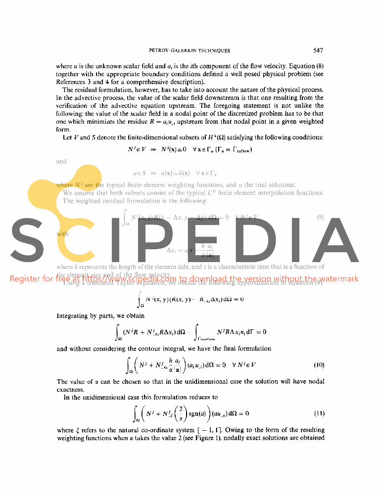
The value of a can be chosen so that in the unidimensional case the solution will have nodal exactness.

In the unidimensional case this formulation reduces to

jn (N' + (:) sgn(a)) (au,,)dQ = 0

where 5 refers to the natural co-ordinate system [ - 1, 11. Owing to the form of the resulting weighting functions when a takes the value 2 (see Figure l), nodally exact solutions are obtained

548 C. E. BAUMANN, M. A. STORTI AND S. R. IDELSOHN

Figure 1. Weighting functions

Figure 2. Sketches of the form functions: (a) node i - 1; (b) node i; (c) node i + 1; (d) compund weighting function for the node i - 1; (e) compound weighting function for the node i + 1

no matter how much different in length the elements may be. Therefore the optimal value of CI to

be used in equation (10) is 2. With the insight gained in the one-dimensional case, we can see that, for the two-dimensional

case, the following formulation,

at. axj bi = a j - , Jbl = (bibi)’/’

in which r i refers to the ith natural co-ordinate, will give nodally exact solutions for those flows parallel to the mesh directions, no matter how much different the sides of the elements may be. In any other situation, the approximation will be much better than the one of equation (10).

When adaptive refinement is used, neither equation (10) nor equation (12) is optimal for the irregular nodes if in the assemblage process the contribution of an irregular node is one-half for each one of its neighbours (as is advocated in Reference 5). When there are irregular nodes in the one-dimensional case, nodal exactness is obtained if the following weighting functions are used for all those elements that share an irregular node:

kj = ( ~ j + 2 ~ ! , sgnfa)) ( j = 1,2)

In Figures 2(a), 2(b) and 2(c) we have the sketches of the form functions for the nodes i - 1 and i + 1 respectively, where the node i is irregular. In Figures 2(d) and 2(e) are represented the compound weighting functions of the nodes i - 1 and i + 1 after the normal assemblage process, that is, one-half of the ith weighting function for each one of its neighbours.


With regard to these modified form functions, we can see that by using their counterpart in the two-dimensional case (only for the irregular node and its two neighbours) a good improvement is obtained.

1.3. Multidimensional compressible Euler equations

A Petrov-Galerkin formulation will be presented and it will be shown how it reduces exactly to the already known formulations of both the scalar case and the case of systems, in the bidimensional and one-dimensional cases respectively. Considering

and

it follows that B. A.- atj

axi J I

Let V' and S' denote the finite-dimensional subsets of H'(R) satisfying the following conditions,

Nie V' * Ni(x)&0 only when xE(rinflow with Mach > 1)

and

u j ( u l , u2, u3, U 4 ) € s i - uj(x)eiqx) m r U i

where Ni is the typical finite element weighting function, U i the ith component of the trial solutions in conservation variables and the function Gi(x) the Dirichlet b.c. for the ith Component of the primitive variables.

We assume that both subsets consist of the typical CO finite element interpolation functions. The proposed Petrov-Galerkin formulation is the following (without the contour terms, see

Reference 6):

(NJ + NI,JBg(BTB)-1'2)(AjU,i)dR = 0 VNie V i (13)

where

Nj = diag(N{, N i , N:, N : )

and

1.4. VeriJications

1. One-dimensional symmetric advective systems. The Euler equations of Gas Dynamics do not constitute a symmetric system when they are

written in terms of conservation variables. For many physical systems of equations, however, a change of variables exists so that they can be written in symmetric form, see References 7-9.

550 C. E. BAUMANN, M. A. STORTI A N D S. R. IDELSOHN

In this code, the entropy variables (as the variables resulting from the symmetrizing change of variables are referred to) were used only at the element subroutine level, whereas primitive variables were used at global levels.

From the condition of symmetry,

A = At = @A#-' =

then

Using

we obtain the already known formulation, i.e.

h l n ( N ' + N!,-(sgnA))(AU,,)dSt=O 2 V N ~ E Y '

2. Bidimensional scalar case.

Using

(B'B)-'/' = (bibi)-'/' = 1bI-l

we obtain once more the formulation sought, i.e.

j Q ( N j + N!61b l lb l - ' ) (a iu , i )dR = 0 V N ~ E V

Note. Considering a two-dimensional system that could be simultaneously diagonalized, we can see that each equation of the decoupled system is a two-dimensional scalar advective equation. Therefore, we can apply the latter verification to each component, and thus we have verified once more the comprehensiveness of this formulation.

1.5. Shock capturing concept

I s.1. Bidimensional scalar advective equation. The SUPG formulation for the bidimensional scalar advective equation was written as follows:

In ( N j + N ! s l b l l b ) - ' ) ( a i u , i ) d R = 0 V N ~ E V

The one-dimensional case has the bidimensional characteristic Vru 11 b, but in the bidimensional case we have b = bll + bl , and only by Vcu = 0. It follows that the foregoing formulation can be written in the following way:

In [Njb'V,u + (V,Nj)'b, - 1 b/, V c u + (V,Nj) 'b l l

Ibl


The third term is not the optimal value because the one-dimensional analogy calls for the value

A way of adding only the necessary artificial diffusivity is to introduce the so-called shock capturing term

After the introduction of the above term, the final formulation is the following:

VN'E V

A comprehensive description of the shock capturing concept for the linear scalar advection-diffusion equation and the multidimensional advective-diffusive systems can be found in References 4 and 10 respectively.

1 s.2. Multidimensional first-order systems of hyperbolic equations. As was done for the scalar case, the Jacobian matrices are split in the following way:

Ai = Aill + Ail ( i = 1 , . . . , nsd)

so that

and

It follows that Al l is an operator of rank 1 that acts only in the direction of the gradient. We can define the operator All as follows,

and, following the development in natural co-ordinates, we define

from which the shock capturing part of the formulation is the following:

r

where


Because BiIBII has rank 1, its negative square root is defined in its non-degenerate subspace, namely

(BjlBll)-1'2 = JLJ- ' 4 #

where I I and 4 are the result of the following eigenproblem:

(BIIBII - 1'1) 4 = 0

Substituting

in the eigenproblem, we get

( A . v u ( ~ ~ I ~ ( A - v u ) ' - n 2 r ) + = o

The solution to this eigenproblem is

4 = A-VU and. ,Iz = ( f i ( 2 ( A - V U ( 2

It follows that

and now, the shock capturing part of the formulation is

Again, as was done for the two-dimensional scalar case, we must subtract from the above expression a quantity equal to the contribution of the plain SUPG in the direction of VU.

From equation (13), the contribution of the plain SUPG is

where

(A - VU)'(BB')-1'2(A * VU)

(A.VUI2 a =

Therefore, the final expression for the shock capturing operator is the following:

2. DISCRETIZED EQUATIONS

In this section we give a description of some important aspects concerning the implementation and use of the method we are dealing with.


2.1. Weighted residual formulation for the compressible Euler equations

The Euler equations can be written in conservation form as follows:

where

UiUi e = & + -

2

Here, e is the total energy and E is the internal energy per unit mass. In order to complete the system we must specify an equation of state p = p ( p , E). Any equation

of this kind may be used, but the equation of a perfect gas is currently used for transonic and supersonic calculations, i.e.

P = (Y - 1)PE

where y is the ratio of specific heats.

it follows that (see Reference 2) The flux vector F j ( U ) is a homogeneous function of degree one in the conservative variables U;

Fj(U) = AjU

and

Fj, j = A j U , j

Let n = ( n l , n2) be the outward unit normal vector on the boundaries and let Fj be split in the following way:

Later we will make reference to

554 C. E. BAUMANN, M. A. STORTI AND S . R. IDELSOHN

Consider a discretization of Q into element subdomains Qe, e = 1, . . . , nel, where nel is the number of elements. We assume

nsl nei

a = ( ) @ , e = l e = 1

Also let re be the whole boundary of element e, r the boundary of R and rint the following set:

rin, = U re - r (::: ) The boundary of the domain Q is assumed to be decomposed as follows:

r = rui U rfi U rslip, 0 = rui n rfi

where Tu, refers to that part of the boundary on which a Dirichlet-type b.c. is specified for the ith component of the primitive variables (i.e. p , u l , U’, p) , Tf , to that part on which no b.c. is specified for the ith component, and rslip to that part on which the natural b.c. F;’) = 0 is specified.

The only natural b.c. is Fi’) = 0 on rslip, because on the inflow/outflow part of the boundary only Dirichlet b.c. are specified for a number of primitive variables (i.e. p , ul , U’, p ) according to the nature of the boundary (inflow/outflow) and to the Mach number. This point will be explained later in this section.

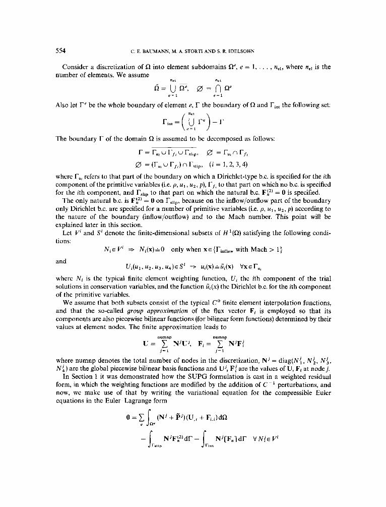
Let V’ and S’ denote the finite-dimensional subsets of H’(f2) satisfying the following conditions:

Nie V’ Ni(x)=O only when X E {rinflow with Mach > l}

and

where Ni is the typical finite element weighting function, Ui the ith component of the trial solutions in conservation variables, and the function Gi(x) the Dirichlet b.c. for the ith component of the primitive variables.

We assume that both subsets consist of the typical CO finite element interpolation functions, and that the so-called group approximation of the flux vector Fi is employed so that its components are also piecewise bilinear functions (for bilinear form functions) determined by their values at element nodes. The finite approximation leads to

ui (u l , U’, u 3 , u 4 ) E s i - ui(x)=qx) v x E r u i

numno numnn

U = E’ ~ j u j , F~ = 1’ N ~ F ; j = 1 j= 1

where numnp denotes the total number of nodes in the discretization, NJ = diag(Ni, N i , N : , N $ ) are the global piecewise bilinear basis functions and Uj, Fi are the values of U, Fi at node j .

In Section 1 it was demonstrated how the SUPG formulation is cast in a weighted residual

form, in which the weighting functions are modified by the addition of C perturbations, and now, we make use of that by writing the variational equation for the compressible Euler equations in the Euler-Lagrange form

0 = 1 J (Nj + ?)(U,, + Fi,’)dQ e Re


in which N j = diag(N{, N i , N < , N i ) , and the Euler-Lagrange equations are the following:

U,, + Fj,j = 0 on R governing equation

Fi2' = 0 on Tslip null flux condition

[F,] = 0 on Tint continuity condition

In the latest equation, the square brackets represents the jump of F, across the interelement boundary. In fact, this equation is automatically verified because F, has CO continuity. Integrat- ing by parts, we obtain the weak form of the weighted residual equation

0 = c pJ(U,, + Fi.JdR + 1 (NjU,, - NliFi)dR e e

r r

Using the following splitting,

we can write

0 = 1 J (Nj + Pj)U,,dR + C J (PjFi,' - NliFi)dR

+ s N j F i l ) d T + J NjF,dT VN~EV

e Re e Re

rsllp rinioutriow

Making use of the forward Euler scheme in the time discretization, we can write the complete formulation in matrix form as follows:

0 = MAb - (At)R

where M is the consistent mass matrix, R the residue and Ab the vector of nodal variations of the conservation variables. The use of the consistent mass matrix is not the one consistent with the developments of Section 1, and on the other hand, it is more CPU-tme consuming; therefore, a lumped mass matrix was used instead.

Any variation in the conservation variables (Ab) is related to the variation of the primitive variables (AS) by a well-known triangular matrix, i.e.

AS = D - ~ A ~

Now considering the nodal vector of primitive variables (a), it is updated after each iteration as follows:

- a{+l = a! + G j D i ' Abj ( j = 1 , . . . , Numnp)

where Gj is the identity matrix for internal nodes, and for boundary nodes it is a special rectifying matrix with absorbing characteristics (see Reference 11).

556 C. E. BAUMANN. M. A. STORTI A N D S . R. IDELSOHN

2.2. Stability, convergence and boundary conditions'

The SUPG method applied to the 1-D-advection equation in a uniform mesh gives

Ata C = -, 6 = sgna

Ax u:+l = U: + C(ufpa - U:),

Let the mesh be of uniform length, and the solution have the form

U: = Pt i , with = 1 (15)

then the amplification coefficient is obtained by substituting equation (15) in equation (14); this coefficient is

(16) I = 1 + q 5 - a - 1)

2.2.1. Stability condition. To have conditional stability we must find an upper bound for At such that

)AI d 1, V l t l = 1 and C d C,,, (17)

The geometrical interpretation of equation (17) is that il (point B) lies on the line joining 5 -' and the point (0, l), and that

-

== BC c AC

As tP6 lies in the unit circle, we conclude that the scheme is stable if C d 1 and unstable otherwise, that is

c d c,,, = 1 (18)

The locus of A({) is a circle of radius C and centre at (1 - C, 0).

2.2.2. Convergence by damping. Supposing that the scheme (14) is utilized to capture the steady solution, each 5 component of the error is multiplied by A in each iteration, and therefore, to reach as fast as possible the steady state, we must look for the C that minimizes \ill. As for any 5, 121 is the distance from B to the origin, it is evident that 121 is minimum when C = 0.5.

To estimate the rate convergence of this algorithm, we use the fact that the maximum of

(ilIc=112 is given by the maximum wavelength admissible by the mesh, namely

then

and

7c2 7c2 I T 2

2N 4N2 4N2 = 1 - 7 + - + O(N-4) = 1 - __ + O(N-4)

PETROV--GALERKIN TECHNIQUES 557

To reduce this component by a factor E, we must iterate n times so that

[AIn = &

Taking logarithms on both sides and using equation (22), we get

-log 1 - __ + O ( N - 4 ) = log& 2 ( d2 1

8N2 n =

7c2 log (1/&)

(241

2.2.3. Absorbent boundary condition. For the last node of the mesh (node N), the SUPG method gives the following equation:

(26) p + l - , n N - dN + 2c(uk-, - U;)

The limit of stability for this equation is C = 0.5. If C were chosen equal to 1, and up = ( - l)i, it can be shown that

U; = (2n + 1)( - 1)” (27)

and here, there is a clear instability in the node N . This instability is not propagated into the domain because in this case nothing can be propagated upstream. However, if this scheme is applied to systems with any characteristic velocity directed inward at the boundary, instabilities generated only at boundary level couple with the components whose characteristic velocity introduces the boundary conditions into the domain, and the scheme is globally unstable. Fortunately, this problem can be solved by taking the mass of the boundary nodes twice as much as the real value. The resulting equations are

u;++1 = U; + C(uk-6 - U;) (28)

The limit of stability for the boundary nodes is now C = 1, and we have the same limit for all the nodes.

2.2.4. Convergence by absorption at the downstream boundary. For C = 1 the scheme is not dissipative at all, there is no dispersion and the error is propagated downstream at a rate of 1 element per time step. As the perturbation is completely absorbed in the downstream boundary, it takes N iterations to eliminate the error. For C < 1, it can be shown that the scheme is O(N/C) because the group velocity for large wavelengths is C elements per iteration.

Contrasting this rate of convergence with the rate of convergence by damping, we can see the best choice is the maximum C compatible with stability.

2.2.5. 1-ll systems. When the forward Euler scheme is used in the temporal discretization, the SUPG method applied to 1-D linear systems gives (in the basis of eigenvectors of A):

Here, 6 = sgn A, gives the correct upwind, and the stability limit for the time step is


The number of iterations needed to carry the component p through N elements is

N h N h n = - = -

AtIk,l AW,I

which is maximum for the lowest eigenvalue, that is

N h

Atmin{ IA,l} n =

Using the maximum At, we have

N max { 14J} min I 14 I )

n =

For the 1-D Euler equations, we have

therefore

M + l

min{M, IM - I I} n = N

(33)

(34)

(35)

The convergence is very low for:

(i) incompressible case: M = E

2 (ii) transonic case: M = 1 -t E n = N -.

n = N/E;

E

2.3. The proposed scheme

accelerate the convergence. For 1-D systems we choose the temporal term Because only the steady solution is of our concern, we can modify the temporal term to

where a is an arbitrary velocity scale to be absorbed by the time step. Straightforward application of the SUPG method to the spatial part of this equation leads to the following equation for the ith node,

and in the basis of eigenvectors of A, equation (37) takes the form

C-'($'+l CI - * ~ i ) = ~ ~ s g n ( ~ p ) ( $ w , i - l - + F , i + I ) + ( $ # , i + l - W p i + $wi-i)}' (38)

(39) - $ i i = C(+vi-a,, - $ w i )

where

6, = sgn(4l)

From equation (39) we can see that all the components t,bw propagate with the same group velocity, that is, C elements per time step.


For the boundary nodes, this scheme gives a completely absorbent boundary condition in the eigenvectors basis, that is

where II + is the diagonal projection matrix

n + = diag(B(A,), &A,), . . . , O(A,)) (41)

in which B(x) = (x + / x l)/2. Transforming back to U variables, we get, from equation (40),

where

In the case of nd > 1, we take / A / as

In the diagonalizable case it can be shown that all the group velocities are optimal (i.e. lvGpl = O(h/At)). The boundary condition previously specified is completely absorptive for waves with incidence normal to 82, i.e. k 11 i? at di2.

This b.c. was implemented in the following way: the absorbent boundary conditions for the decoupled system was

$K1l = $ % + I + H+($% - $nN+1) (45)

II + is a projection operator onto the eigenvectors with positive eigenvalues. Coming back to the U variables,

U%z'i = U%+i + (IAIN++l)-lRiv+l (46)

But, in practice one can fix only the primitive variables, so that the real boundary conditions are (in the $ basis):

(47) n + 1 -

$N+1 - $ % + l + (S-'n'S)($% - $nN+l)

where II' is the projection operator used in the primitive variables and S is the change of basis matrix. In general, the resulting projection matrix

riff = S-lnfs (48)

will not be diagonal in the $ basis, so that different components are mixed by the boundary condition. Furthermore, the resulting boundary condition could not be stable.

However, for supersonic flow, both matrices ll and II' are the identity matrix in the downstream boundary and the null matrix at the upstream boundary so that (38) reduces to (35) and the resulting boundary condition will be stable and absorbent (at least for the linear range).

2.4. Boundary conditions

depends upon the local Mach number. The number of primitive variables to be specified on the inflow/outflow part of the boundary


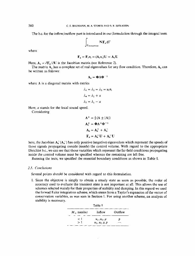
The b.c. for the inflow/outflow part is introduced in our formulation through the integral term

1 NF,dT rinioutrlow

where

F, = Fini = (Aini)U = A,U

Here, A, = dF,/dU is the Jacobian matrix (see Reference 2).

be written as follows: The matrix A, has a complete set of real eigenvalues for any flow condition. Therefore, A, can

A, = @A@-'

where A is a diagonal matrix with entries

,I1 = & = ,I3 = Mini

,I4 = 1, + a

As = ,I1 - a

Here, U stands for the local sound speed. Considering

A * = * ( A 1A1)

A: =@A'@-'

A, = A: -+ A,

F, = A;U + A i U

here, the Jacobian A; (A,) has only positive (negative) eigenvalues which represent the speeds of those signals propagating outside (inside) the control volume. With regard to the appropriate Dirichlet b.c., we can see that those variables which represent the far-field conditions propagating inside the control volume must be specified whereas the remaining are left free.

Running the tests. we specified the essential boundary conditions as shown in Table I.

2.5. Conclusions

Several points should be considered with regard to this formulation.

1. Since the objective is simply to obtain a steady state as soon as possible, the order of accuracy used to evaluate the transient state is not important at all. This allows the use of schemes selected mainly for their properties of stability and damping. In this regard we used the forwad Euler integration scheme, which stems from a Taylor's expansion of the vector of conservation variables, as was seen in Section 1. For using another scheme, an analysis of stability is necessary.

Table I

M , number Inflow Outflow

PETROV-GALERKIN TECHNIQUES 56 1

2. It appears from the formulation that the natural b.c. of null flux on slip boundaries would have to be verified, in the weighted form, in the same way that the flow of heat is where null flow is specified as a natural b.c. of a heat transfer analysis. However, this proved to be a most unstable b.c., not being verified at all and spoiling the solution. A large number of schemes for the analysis of inviscid compressible flows appear to have the same shortcoming (see References 12- 14).

The code avoids this shortcoming, evaluating automatically for each node of the declared slip boundaries, a unit vector ii’, thus taking into account the orientations and lengths of the elements’ sides that converge to the jth node and that are part of the slip boundary, i.e.

.”! = jrs,ip Njnidr ( il ( jrs,*p Njnl dT Y)-’‘* Then, after each iteration, the velocities are modified as follows:

v’ = VJafte, - (iij Vjafter)iij iter. iter.

where Vifter is the velocity in thejth node obtained from a;+ and Vjis the new value of this

velocity to be assigned to a;+ 1.

3. If we consider that the rate of convergence is given by the CFLN and that the meshes have in

general highly variable element sizes, it is understood why the convergence is speeded up when the optimum time step is used for each node. This code automatically uses a nodal time step that is in accordance with a specified CFLN; we usually specify CFLN = 0.9. This CFLN is reduced for those nodes that are on the boundary because of stability, the reduction being indirectly accomplished by using an augmented lumped mass matrix.

4. Because the steady state is our target, we can use a sequence of meshes. The coarser a mesh, the cheaper it is to obtain an approximated solution. Therefore, we begin with a coarse mesh and when the rate of convergence decays an automatic switch is made to a finer mesh.

With regard to the automatic refinements one can choose between an overall refinement or a localized (adaptive) refinement. As a matter of fact, the first ones are always overall refinements, while the adaptive ones are used in the final stages of refinement.

5. Any type of upwind introduces artificial diffusivity. The diffusivity acts in the zones of high gradients, no matter what is the origin of such gradients; as a result, there may be zones in which spurious generation of entropy occurs (e.g. the stagnation zone generated by a blunt body). The straightforward procedure for avoiding such errors is to use adaptive refinement in those zones.

iter.

3. NUMERICAL RESULTS

3.1. Some preliminary results for the 1-D Euler equations

The proposed scheme was applied to the Euler equations (non-linearized) in the subsonic regime ( M = 0.1,0.5), transonic ( M = 1.05) and supersonic ( M = 2). The mesh has 20 elements (21 nodes). The At was chosen always such that C = 0.9 for the greatest eigenvalue.

3.1 . I . Boundary conditions. The boundary conditions were:

(i) subsonic case ( M = 05, 01): M = U , p = 1.4 for the first node, p = 1 for the last node; (ii) supersonic case ( M = 1.05,2): U = M , p = 1.4, p = 1.0 at the first node, no conditions at the

last (downstream) node.

562 C . E. BAUMANN, M. A. STORTI AND S. R. IDELSOHN

3.1.2. Results.

1. In the supersonic case there is no ‘mixing’ in the components. We mean by this that a perturbation in pressure is not transferred to the velocity or to the density components. This is a consequence of the fact that all components move with the same group velocity and in the same sense.

2. Comparing the two methods for M = 2, we see that for the proposed scheme the perturbation travels with no dispersion and with a velocity of 0*9h/At.

3. For M = 1.05, running the standard scheme (Figure 3), we have a strong perturbation which travels downstream with velocity U - c = 0.05. The fact that for node 3

6 p 0.0367 c-2 - = N l

6p 0.035 - N

I I I

Figure 3. Pressure perturbation for the standard scheme

Pressure

I I 1

Figure 4. Pressure perturbation for the proposed scheme


and

p6v 1.4 x 0.0245

cbp 1x00355 xl _- -

confirms that it is a pressure wave. With the proposed scheme all the components travels with the same velocity (Figure 4).

4. For all the subsonic cases, there is mixing of components, even with the proposed scheme. That is because the eigencomponents corresponding to both U + c and U travel downstream at the same velocity and are partially reflected at the downstream boundary, which results in a perturbation of the U - c eigencomponent which travels upstream, and again there is a reflection at the upstream boundary, and so on. If the overall gain of this process is greater than one the scheme is unstable. This effect can be observed in several cases.

3.2. Evaluation of an oblique shock wave

We present a problem of which we know the analytical solution; it consists in the evaluation of an oblique shock wave originated when a flow incident over a wedge (see Figure 5). This problem has already been used to test several schemes.I5 As a result of the obliqueness of the shock with the mesh, this test enables us to check the capability of this scheme to evaluate this kind of shock.

The mesh consists of 20 x 20 elements homogeneously distributed over the domain (a unit square).

At the inflow [A-B-C] all variables were specified ( M > 1). The wall [D-A] was specified as slip boundary so that the code could rectify the velocities of all those nodes lying on that boundary. For this domain we could have imposed the null flux on [D-A] by restraining the corresponding d.0.f. (u2 = 0), but for general curved surfaces this solution is not practical, and one necessarily has to rely on the declaration of slip boundary.

No variable was fixed either on the outflow [C-D] or on the slip boundary [D-A]. The

boundary condition to be imposed in the node A is not unique, but anyway, the values of the state variables after the shock and the angle of the shock itself will not be affected.

( p = 1.0

~1 =0.98481

U Z = -0.17365 inflow ( M = 2)

(p =0178596

Point of J view

A

Figure 5. Oblique shock wave

5 64 C . E. BAUMANN, M. A. STORTI A N D S . R. IDELSOHN

Figure 6. Density elevation on the oblique shock wave

The result is the following:

( p = 1.458

u1 =0887

U2 = 0.000 outflow (M = 1.64)

( p = 0.304

Figure 6 shows this result in the form of density elevation (in Figure 5 is indicated the observation point). We can see that a sharp shock without oscillations was obtained. With regard to the numerical values, we can say that there was complete agreement between the numerical and the analytical values.

3.3. Calculations for the NACAOO12 airfoil

Two test cases were chosen; both are lifting flows. The first of them is the ubiquitous case M , = 0.80 with an angle of attack = 1.25 deg, and the second test has M , = 1.20 and an angle of

attack = 7.00 deg. These are two of the cases considered in the AGARD Fluid Dynamics Panel Working Group

07 (see Reference 16).

3.3.1. Meshes. Figure 7 shows the final mesh for the first test and Figure 8 that one of the second test. Each one was obtained from an initial coarse C-mesh that was automatically refined. In the coarser C-meshes, the convergence was very fast and the evaluation of the residue very little time consuming. As the C-meshes became finer, the convergence became slower and the evaluation of the residue more time consuming. The mesh was overall refined when the rate of convergence decayed too much.

Only the final stages of refinement were of adaptive type. In this case, the gradients of the pressure were used as the criterion to switch the adaptive refinement. At the interfaces of different mesh sizes the continuity is maintained by elimination of internal nodes, e.g. by sharing the forces between the adjacent nodes.

In fact, the refinement technique was introduced in the code in his simplest way. It is the object of current researches and it is not considered in the scope of this paper.


Figure 7. NACA0012 Airfoil: final mesh, first test

L"

Figure 8. NACA0012 Airfoil: final mesh, second test

3.3.2. Initial and boundary conditions. Each case was initialized with a uniform freestream flow at the prescribed Mach number and angle of attack.

For the first case the initial conditions are p = 1.0, u1 = cos(l.25), u2 = sin(1.25), and p = 1.1 1607 everywhere.

The boundary conditions are the following: (1) Slipping boundary condition on the airfoil. (2) Imposition of p, u1 and u2 on the inflow part of the domain. (3) Imposition of p on the outflow part.

For the second case the initial conditions are p = 1.0, u1 = cos(7.0), u2 = sin(7.0), and p = 0.49603 everywhere.

The boundary conditions are the following: (1) Slipping boundary condition on the airfoil. (2) Imposition of p, u l , u2 and p on the inflow part of the domain.

566 C . E. BAUMANN, M. A. STORTI A N D S. R. IDELSOHN

I 8 7 5

I 1 9 8

1721

I 6 4 5

I 5 6 8

1491

I414

1 3 3 1

I 2 6 0

1183

I )06

I O Y )

0 953

0 816

0 799

0 722

0645

0 568

Figure 9. NACA0012 Airfoil pressure contours, first test

I 3 5 5

1280

I 204

I128

I 0 5 3

0977

0 90t

0826

0750

0 614

0599

0 5 t 3

0 4 4 1

0 372

0 296

0 220

0145

0 0 6 9

L Figure 10.

12

08

04

8 00 1

- 04

-0 8

- 1 2

NACA0012 Airoil: Mach contours, first test

0 04 08 12 CHORD

Figure 11. NACA0012 Airfoil C , distribution, first test


L Figure 12. NACA0012 Airfoil: pressure contours, second test

IY " U

Figure 13. NACA0012 Airfoil Mach contours, second test

3.3.3. Results. Figures 9-1 1 show pressure contours, Mach contours and C, distribution for

the first case, whereas for the second case, the pressure and Mach contours are shown in Figures 12 and 13 respectively.

The numerical results are in good agreement with those reported in Reference 16. Only in the first test case is there a slight difference in the positions of the shock waves; the positions given by this code are slightly downstream when compared with those given in Reference 16.

3.4. Conclusions

The numerical solution for the wedge problem and the airfoil calculations show that this SUPG version gives very good shock resolution and values of the state variables for steady state computations.


With regard to the CPU time, we acknowledge that this finite element code is much slower than a finite difference code provided that a structured grid could be fitted. When a structured grid can not be fitted, this code still can solve the problem, no matter how complicated the domain or the boundary conditions may be.

ACKNOWLEDGEMENTS

The authors wish to express their gratitude to CONICET for its financial support. They also wish to thank Nestor Aguilera and Norberto Nigro for helpful comments, and to Karl for his

outstanding job in typing the manuscript.

REFERENCES

1. J. Donba, ‘A Taylor-Galerkin method for convective transport problems’, Znt. j . numer. methods eng., 20, 199-259 (1984).

2. T. J. R. Hughes and T. E. Tezduyar, ‘Finite element methods for first-order hyperbolic systems with particular emphasis on the compressible Euler equations’, Comp. Methods Appl. Mech. Eng., 45, 217-284 (1984).

3. T. J. R. Hughes, L. P. Franca and G. M. Hulbert, ‘A new finite element method for computational fluid dynamics: VIII. The Galerkin/least-squares method for advective4iffusive equations’, Comp. Methods App l . Mech. Eny., 73,

4. T. J. R. Hughes, M. Mallet and M. Mizukami, ‘A new finite element method for computational fluid dynamics: 11. Beyond SUPG, Comp. Methods Appl. Mech. Eng., 54, 341-355 (1986).

5. P. Devloo, J. T. Oden and T. Strouboulis, ‘Implementation of an adaptive refinement technique for the SUPG algorithm’, Comp. Methods Appl. Mech. Eng., 61, 339-358 (1987).

6. T. J. R. Hughes and M. Mallet, ‘A new finite element method for computational fluid dynamics: 111. The generalized streamline operator for multidimensional advection-diffusion systems’, Comp. Methods Appl. Mech. Eny., 58,

7. A. Harten, ‘On the symmetric form of systems of conservation laws with entropy’, J . Comp. Phys., 49, 151-164 (1983). 8. E. Tadmor, ‘Skew-selfadjoint forms for systems of conservation law’, J . Marh. Anal. Appl., 103, 428-442 (1984). 9. T. J. R. Hughes, L. P. Franca and M. Mallet, ‘A new finite element method for computational fluid dynamics: I.

Symmetric forms of the compressible Euler and Navier-Stokes equations and the second law of thermodynamics’, Comp. Methods Appl. Mech. Eng., 54, 223-234 (1986).

10. T. J. R. Hughes and M. Mallet, ‘A new finite element method for computational fluid dynamics: IV. A discontinuity- capturing operator for multidimensional advective4iffusive systems’, Comp. Methods Appl. Mech. Eng., 54,223-234 (1 986).

1 I . C. E. Baumann, M. A. Storti and S. R. Idelsohn, ‘Absorbing boundary conditions for the solution of transonic flows’, GTM internal communication.

12. J. T. Oden, T. Strouboulis and P. Devloo, ‘Adaptive finite element methods for the analysis of inviscid compressible flow: Part I. Fast refinementjunrefinement and moving mesh methods for unstructured meshes’, Comp. Methods Appl. Mech. Eng., 56, 327-362 (1986).

13. C. Koeck, ‘Computation of three-dimensional flow using the Euler equations and a multiple-grid scheme’, fn t . j .

numer. methods Juids, 5, 483-500 (1985). 14. M. S. Engelman, R. L. Sani and P. M. Gresho, ‘The implementation of normal and/or tangential boundary conditions

in finite element codes for incompressible fluid flow’, Int. j . numer. methods Juids, 2, 225-238 (1982). 15. S. F. Davis, ‘A rotationally biased upwind difference scheme for the Euler equations’, J . Comp. Phys., 56,65-92 ( I 984). 16. T. H. Pullimam and J. T. Barton, ‘Euler computations of AGARD Working Group 07 Airfoil Test Cases’, .41AA

17. M. A. Storti, C. E. Baumann and S. R. Idelsohn, ‘Stability analysis for the calculation of transonic flows with

173-189 (1989).

305-328 (1986).

Paper 85-0018, 1985.

SUPG-type schemes’, GTM internal communication.

Improving the convergence rate of the Petrov-Galerkin ... · international journal for numerical...

Documents

Transcript of Improving the convergence rate of the Petrov-Galerkin ... · international journal for numerical...