Improving the confidence of “questioned versus known" fiber

comparisons using microspectrophotometry and chemometrics

Georgina Sauziera,b, Eric Reichardc, Wilhelm van Bronswijka, Simon W. Lewisa,b and John V.

Goodpasterc,*

a Department of Chemistry, Curtin University, GPO Box U1987, Perth, Western Australia, 6845.

b Nanochemistry Research Institute, Curtin University, GPO Box U1987, Perth, Western Australia, 6845.

c Department of Chemistry and Chemical Biology, Indiana University Purdue University Indianapolis (IUPUI),

Indianapolis, IN 46202. E-mail: jvgoodpa@iupui.edu.au; Tel: +1 317 274 6881

*Author for correspondence

Author e-mails:

Georgina Sauzier: Georgina.Sauzier@postgrad.curtin.edu.au

Eric Reichard: reicharde@yahoo.com

Wilhelm van Bronswijk: W.vanBronswijk@curtin.edu.au

Simon W. Lewis: S.Lewis@curtin.edu.au

John V. Goodpaster: jvgoodpa@iupui.edu

Abstract Microspectrophotometry followed by chemometric data analysis was conducted on pairs of

visually similar blue acrylic fibers, simulating the “questioned versus known” scenarios often

encountered in forensic casework. The relative similarity or dissimilarity of each pair was

determined by employing principal component analysis, discriminant analysis and Fisher’s

exact test. Comparison of fibers from within each set resulted in a correct inclusion result in 10

out of 11 scenarios, with the one false exclusion attributed to a lack of reproducibility in the

spectra. Comparison of fibers from different sets resulted in a correct exclusion result in 108

of 110 scenarios, with two sets that shared identical dye combinations being indistinguishable.

Although the presented methods are not infallible, they may nonetheless provide a path forward

for forensic fiber examiners that has a more scientifically rigorous basis on which to support

their findings in a court of law.

Keywords: Forensic science, textile fibers, microspectrophotometry, chemometrics ___________________________________________________________________

This is the author's manuscript of the article published in final edited form as:Sauzier, G., Reichard, E., van Bronswijk, W., Lewis, S. W., & Goodpaster, J. V. (2016). Improving the confidence of “questioned versus known” fiber comparisons using microspectrophotometry and chemometrics. Forensic Chemistry, 2, 15–21. https://doi.org/10.1016/j.forc.2016.08.001

1. Introduction Textile fibers are a commonly encountered form of forensic trace evidence, and may be used

to provide evidence of association due to their high tendency to shed and be transferred through

physical contact [1-3]. Furthermore, certain classes of fibers can prove highly distinctive based

on their morphology, composition and especially color. Over 7,000 textile dyes and pigments

are currently produced worldwide, with combinations of these often used to impart specific

colors to textile products [2, 4]. Additionally, textile dyeing processes are generally carried out

in batches that may exhibit minor variations in dye form, shade or strength [5]. Although many

colors can be distinguished visually, these assessments are subjective and may be affected by

metamerism or the examiner’s color vision [6, 7]. More objective measurements can be

obtained using instrumental methods such as microspectrophotometry (MSP), which is favored

as a rapid and non-destructive method for characterizing the color of dyed fibers [8, 9]. Several

studies have demonstrated the capability of MSP to distinguish visually similar colored fibers

based upon different chromophores in the molecular structure of their dyes [10-14].

Forensic fiber examinations frequently involve comparisons between a questioned (Q) sample

recovered from a crime scene and a known (K) sample taken from a known source such as a

suspect’s home or belongings [15]. Such comparisons may result in one of three outcomes:

inclusion (e.g., “Q and K may have originated from the same source”), exclusion (e.g., “Q and

K did not originate from the same source”), or an inconclusive result. In the case of textile

fibers, which are mass produced, a “source” can only be described in terms of a class of objects

that share the same physical and chemical characteristics rather than any particular item.

The underlying logic of these “questioned versus known” (Q vs. K) comparisons can be

expressed through the following if/then statement:

“IF Q and K originated from the same source, THEN Q and K will share

indistinguishable class characteristics.”

It follows, then, that the contrapositive must also be true:

“IF Q and K do not share indistinguishable class characteristics, THEN Q and K did

not originate from the same source”.

It is critical to realize, however, that it is a fallacy to affirm the consequent:

“IF Q and K share indistinguishable class characteristics THEN Q and K originated

from the same source”.

This means, therefore, that any forensic comparison that results in an association based upon

indistinguishable characteristics may be a false inclusion. There is also an implicit assumption

for any given Q vs. K comparison that the source(s) of Q and K are homogenous, i.e. that both

the questioned and known are representative samples of their original source(s). If this

assumption is invalid, it may lead to false exclusions (see contingency table below).

RESULT OF COMPARISON

Indistinguishable Characteristics

Distinguishable Characteristics

GR

OU

ND

TR

UTH

Same Source (Q = K)

True Inclusion False Exclusion

Different Sources (Q ≠ K)

False Inclusion True Exclusion

In general, the relative strength of an inclusion depends upon the rarity of the class to which Q

and K are assigned, as the chance of a coincidental inclusion goes down as the source of Q and

K becomes smaller and less common. A more quantitative approach to describing these

outcomes can be expressed by stating two competing hypotheses:

Prosecutor’s Hypothesis (Hp): The questioned fiber(s) originate from the individual/object

which is the source of the known. This hypothesis represents a “true inclusion”.

Defense Hypothesis (Hd): The questioned fiber(s) originate from another individual/object

than the one suspected. This hypothesis represents a “false inclusion”.

In turn, a likelihood ratio (LR), as derived from the Bayes Theorem can be defined as:

LR = P(E | Hp ) / P(E | Hd )

Where evidence (E) can be a quantitative score of similarity or dissimilarity between the

questioned and known, P(E | Hp ) is the probability of observing the evidence given the

prosecutor’s hypothesis and P(E | Hd ) is the probability of observing the evidence given the

defense hypothesis.

Ultimately, a fiber comparison that utilizes an analytical method such as MSP includes a

determination of whether the spectra from a Q and K are truly “indistinguishable”. Such a

determination depends upon the variation between spectra of the questioned and known

samples. Specifically, guidelines published by the Scientific Working Group for Materials

Analysis (SWGMAT) dictate that a ‘spectral inclusion’ can be made if the questioned spectrum

lies within the range of the known spectra in terms of the curve shape and absorbance values

[16].

Traditionally, assessment of whether two or more fibers exhibit similar spectral characteristics

has relied upon an examiner’s visual interpretation of the data. The subjective nature of these

comparisons has led to trepidations regarding potential human error or bias [17]. Substantial

research in recent decades has therefore examined the utility of analytical techniques with

chemometric analysis to provide more objective fiber examinations [18-22]. Liu for example

employed Raman spectroscopy with chemometrics to distinguish cotton cellulose fibers based

upon their color, crystalline fraction and strength [23]. Morgan et al. also described several

inter-laboratory studies employing chemometrics with UV-vis and fluorescence MSP to a large

database of dyed fibers, discriminating fibers according to both their dye composition and

loadings with high levels of accuracy [24]. However, these studies have largely focused on the

simultaneous discrimination of several fibers, rather than the Q vs. K comparisons more typical

of forensic casework. Furthermore, there is presently a lack of quantitative measures for

assessing sample similarity. The establishment of cut-off criteria for an ‘inclusion’ or

‘exclusion’ result would provide an additional statistical basis on which forensic practitioners

could support their findings in a court of law.

This study investigated the potential use of MSP spectroscopy followed by chemometrics to

assess the similarity or dissimilarity of several blue-dyed acrylic fiber sets. Chemometric data

analysis was conducted on spectra acquired from various fiber pairs in order to simulate

casework Q vs. K comparisons. Quantitative determination of the similarity was then made by

comparing the resultant data using hypothesis testing.

2. Materials and methods 2.1 Samples

Fiber samples were provided by the University of South Carolina. The sample population

consisted of eleven sets of bilobal blue acrylic fibers colored with varying combinations of

cationic (basic) dyes, as shown in Table 1. Representative images of each fiber set are provided

in the electronic supplementary information (Figure S1). Fibers from each set had varying

diameters as indicated.

Table 1: Dye compositions of eleven blue acrylic fiber sets utilized in this study.

Fiber Set Dye composition Diameter (µm)

Fiber A Blue 3, Red 18, Yellow 28 17.5

Fiber B Blue 41, Red 46, Yellow 28, Yellow 29 15

Fiber C Blue 41, Red 46, Yellow 28 15

Fiber D Blue 41, Red 29, Yellow 21 21.25

Fiber E Blue 147, Red 29, Yellow 28 23.75

Fiber F Blue 3, Blue 147 23.75

Fiber G Blue 147, Red 46, Yellow 28 18.75

Fiber H Blue 3, Red 18, Yellow 28 22.5

Fiber I Blue 41, Red 29, Yellow 28 22.5

Fiber J Blue 41, Red 18, Yellow 28 25

Fiber K Blue 3, Red 46, Yellow 28 25

2.2 Microspectrophotometry

Individual fibers from each set were randomly removed and mounted on glass microscope

slides using Permount mounting media (Fisher Scientific, U.S.A) for analysis. MSP spectra

were acquired between 400-800 nm using a CRAIC QDI 2000 microspectrophotometer in

transmission mode, operated at 150x magnification. The spectrometer was calibrated using

NIST traceable standards prior to use. An autoset optimization, dark scan and reference scan

were also obtained prior to each sample analysis. Ten fibers were analyzed from each set, with

five spectra recorded along the length of each to account for intra-fiber variation. Fifty averaged

scans at a resolution of 5 nm were obtained for each spectrum.

2.3 Data analysis

Data pre-processing and chemometric analysis was conducted using XLSTAT (AddInSoft,

Paris, France) and Unscrambler X 10.3 (Camo Software AS, Oslo, Norway). All spectra were

first baseline offset to 0 % absorbance and normalized to account for variations associated with

the fiber diameter. In this case normalization to “unit vector length” was chosen as it was

appropriate for UV-vis spectra [25]. Other normalizations were explored (i.e., normalization

to unit area) but the performance of the model was not improved. Principal component analysis

(PCA) was then conducted on the entire dataset of known sample spectra using Unscrambler X

10.3.

The Q vs. K approach was undertaken by conducting PCA on pairs of fiber sets using XLSTAT.

In each comparison, the “known” sample was defined as a group of 45 spectra originating from

the first nine fibers of the set, and the “questioned” sample was defined as the five spectra

acquired from the last fiber analyzed in the same set, or the last fiber analyzed in a different

set. Discriminant analysis (DA) was performed in XLSTAT on each pair based on their PCA

scores against the first three PCs (accounting for > 98 % of total variance in each comparison),

calculating prior membership probabilities from each training set. The number of PCs used to

construct each model was selected according to the corresponding scree plots. All DA

comparisons employed the Mahalanobis distance measure and assumed non-equal covariance

matrices. This approach was repeated for each possible pair of questioned and known samples,

yielding a total of 121 comparisons amongst all eleven fiber sets. Sample similarity was then

evaluated using the classification results of the questioned spectra, mean membership

probabilities and Fisher’s exact test.

3. Theory 3.1 Chemometric methods

Analytical methods such as microspectrophotometry generate a large quantity of multivariate

data, posing difficulties in objective interpretation. This issue can potentially be overcome

through the use of multivariate statistical (chemometric) methods, such as PCA [26-28]. PCA

reduces the dimensionality of complex data by transforming the original set of correlated

variables into a lesser number of new, orthogonal variables referred to as principal components

(PCs) [29-31]. Each successive PC is calculated to describe the maximum proportion of

variation in the dataset that is not described by the previous components, such that the majority

of information is retained within the first few PCs. These PCs may then be used as a new

coordinate system to re-visualize the dataset, revealing patterns or relationships between

samples that would not be readily evident from the raw data alone [32, 33]. Further information

can be gleaned through inspection of the loadings plots, which indicate the variables of the

original dataset that significantly contribute to the separation of samples along each PC [34].

Following the identification of sample groupings within a dataset, it is often of interest to

develop classification models for future samples. This can be done using discriminant analysis

(DA); a technique that builds a mathematical function to maximize the separation between

known classes of samples [35, 36]. The subsequent model can then be employed to assign

unknown samples to the most probable class. As the sample size of each group must exceed

the number of variables, DA is typically carried out following data reduction techniques such

as PCA, with the first few PCs being substituted in place of the original variable set [37, 38].

3.2 Sample similarity metrics

Due to the large size difference between the questioned and known classes, the overall

classification accuracy of the discriminant model could not be taken as a reliable measure of

differentiation. As only five of the 50 spectra involved in each comparison originated from the

questioned sample, an overall classification accuracy of 90 % would be obtained even if all

questioned spectra were assigned to the known class. Similarly, the overall performance of the

discriminant function as expressed by the area under a receiver operator characteristic curve

could still be near unity, despite poor classification of the questioned spectra. The

differentiation between each pair was therefore evaluated according to the percentage of

questioned spectra assigned to the known class, assessing the extent to which the questioned

sample fell within the boundaries of the known source (as recommended by the current

SWGMAT guidelines [16, 39]). In addition, the mean membership probability of the

questioned sample belonging to the known class was recorded.

Fisher’s exact test was then used to obtain a quantitative measure of sample similarity. This

test is useful in the analysis of contingency tables resulting from the binary classification of

objects, such as the classification of spectra as belonging to a questioned or known class.

Fisher’s test calculates the exact probability of observing a given combination of data in a

contingency table, as described below [40, 41]. The null hypothesis (p > 0.05 at the 95 %

confidence level) is that the rows and columns of the table are independent, i.e., there is no

association between the assignation of spectra to the questioned or known fibers and the actual

source of the spectra [42]. This would indicate that the questioned and known fibers possess

overlapping characteristics, and thus could potentially originate from a common source.

Conversely, the alternative hypothesis (p < 0.05) is that there is an association between the

actual and predicted fiber sources. This in turn implies that the questioned and known fibers

are distinguishable, and that they are likely to originate from different sources.

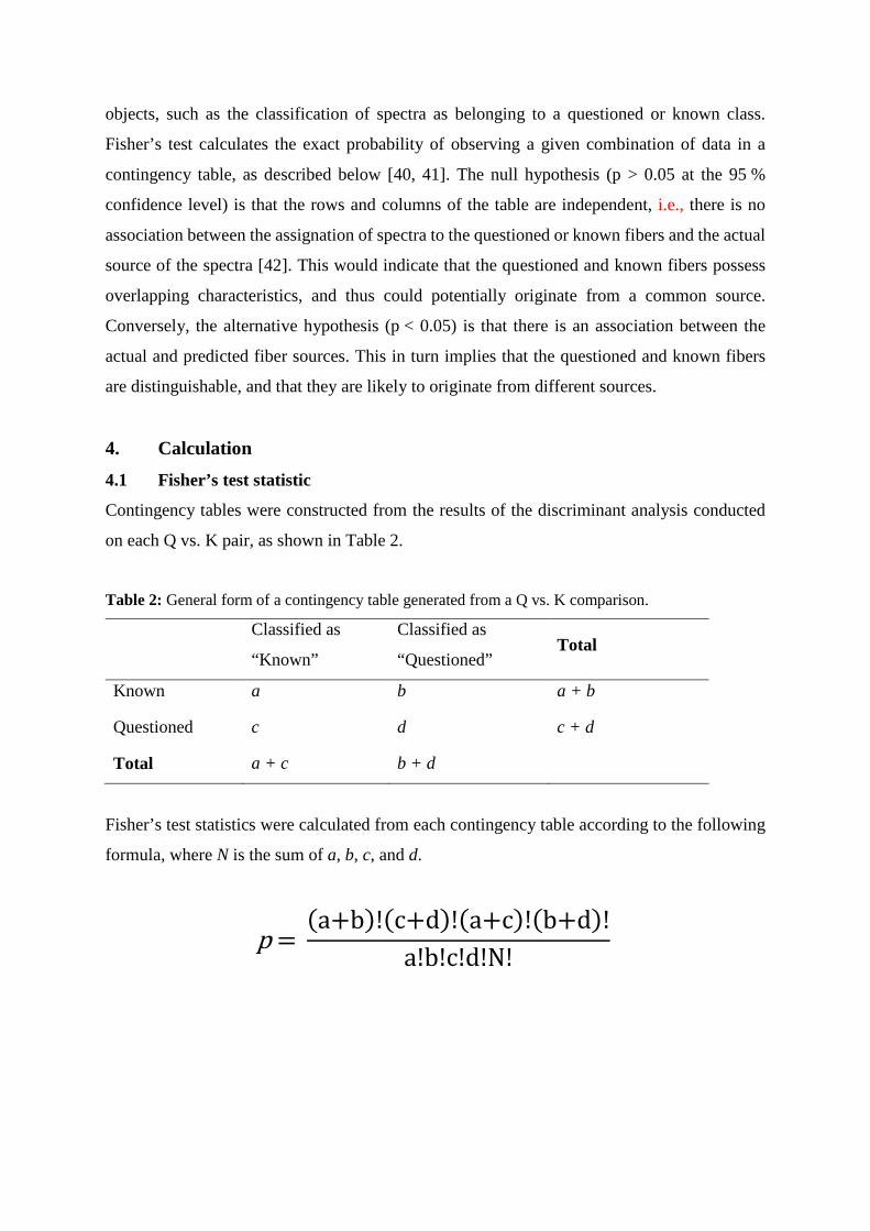
4. Calculation 4.1 Fisher’s test statistic

Contingency tables were constructed from the results of the discriminant analysis conducted

on each Q vs. K pair, as shown in Table 2.

Table 2: General form of a contingency table generated from a Q vs. K comparison.

Classified as

“Known”

Classified as

“Questioned” Total

Known a b a + b

Questioned c d c + d

Total a + c b + d

Fisher’s test statistics were calculated from each contingency table according to the following

formula, where N is the sum of a, b, c, and d.

p = (a+b)!(c+d)!(a+c)!(b+d)!

a!b!c!d!N!

5. Results and discussion 5.1 Preliminary considerations

Single textile fibers often exhibit varying levels of dye uptake, particularly where a

multicomponent dye has been used [5, 6]. This potential heterogeneity both among and within

individual fibers requires appropriate sampling to obtain representative data for the bulk

material. For synthetic textiles such as acrylics, SWGMAT guidelines recommend the

examination of at least five individual fibers, with a minimum of five replicate spectra acquired

for each [15, 16]. In this study, nine to ten fibers were hence utilized in each known set to

ensure representative sampling. As it is not always possible in casework scenarios to recover

multiple fibers from the questioned source, single fibers were chosen to act as the questioned

sample. This was intended to simulate a challenging scenario wherein a single fiber is

recovered and submitted for analysis alongside a much larger known source, such as a garment

or blanket. However, the large difference in size of the questioned and known classes has the

potential to affect the results obtained in this study, and this must be considered when

evaluating the results.

MSP spectra from fiber sets A and H (Table 1) were each collected over two consecutive days,

with the instrument re-calibrated on each date. In a casework scenario, the known and

questioned fibers would ideally be analyzed on the same day, thus minimizing the risk of daily

variations in the instrument performance affecting the results. However, this is not always

feasible where a large number of samples have been submitted for analysis. The re-calibration

of the instrument, in addition to inherent instrumental variability, may therefore result in

spectral deviations that could influence the results determined through statistical analysis.

5.2 Correlation between fiber spectra and component dyes

Chemical structures of the component dyes used in this research are provided in the

supplementary information (Figure S2). Although reference standards for each dye were not

available, visual inspection of the spectra allowed broad correlations to be drawn between these

dyes and specific spectral features (Table 3).

Table 3: Spectral features attributable to dyes contained in the blue acrylic fibers.

Dye Absorbance peak/s

Blue 3 Sharp peak at 655 nm, shoulder at 600 nm

Blue 41 Peak at 625 nm, shoulder at 585 nm

Blue 147 Broad peak at 600 nm

Red 46 Peak at 545 nm

Yellow 21 Peak at 450 nm, possible peak at 425 nm

Yellow 28 Peak at 450 nm

Yellow 29 Peak at 450 nm

For the purposes of this inspection, the fiber sets were divided into three groups according to

their primary blue dye: Blue 3 (sets A, F, H and K), Blue 41 (B, C, D, I and J) or Blue 147 (sets

E and G). Example spectra from each of these fiber sets are shown in Figure 1. It was noted

that spectra from sets A and H appeared visually identical, as expected given their identical

dye combination (Table 1).

Fibers containing Blue 3 exhibited a strong peak at 655 nm with a shoulder at 600 nm,

consistent with known absorbance bands for this dye [43-45]. Sets A, H and K also showed

minor peaks or shoulders at 450 nm consistent with Yellow 28 [46, 47]. No such peak was

noted in the spectrum of set F, as these fibers did not contain any yellow dyes. Set K spectra

exhibited a weak shoulder at 545 nm, possibly due to the presence of Red 46. Red 18, present

in fibers from sets A and H, gave no distinguishable peak in the corresponding spectra. Given

the broad, overlapping nature of MSP spectra, it is possible that any absorbance band from this

dye was masked by the blue or yellow dyes, which would likely have been present at much

greater concentrations.

Samples containing Blue 41 showed a corresponding peak at 625 nm, with a shoulder at 585

nm. It is likely that the latter resulted in the masking of any red dyes, as none of the spectra

yielded observable peaks in the red (500-550 nm) region. Fibers containing Yellow 28 gave

the expected absorbance band at 450 nm, with the exception of sets I and J, which instead

exhibited broad shoulders at ca. 490 nm. It is possible that this band shift is due to the overlap

or interaction between multiple dyes contained in these samples. Fiber set B (containing

Yellows 28 and 29) gave a single peak in the yellow region indistinguishable from that arising

solely from Yellow 28, indicating that these dyes give rise to overlapping bands centred around

450 nm. Set D gave a weak shoulder at ca. 425, consistent with Yellow 21 [47, 48].

Both fiber sets containing Blue 147 produced a single broad band at ca. 600 nm. Any Blue 147

contained in set F could was hence likely masked by the 600 nm shoulder of Blue 3, also

explaining why this shoulder exhibited a broader peak width and greater intensity relative to

the 655 nm peak compared to fibers containing only Blue 3. The Blue 147 peak may also be

responsible for masking any bands arising in the red region due to Red 29 (set E) or Red 46

(set G). Set G fibers gave no distinguishable peak in the yellow region, despite containing

Yellow 28, indicating that the concentration of yellow dye in these fibers was too low to be

detected under the conditions in this study.

Figure 1: Normalized MSP spectra (each averaged across five replicates) for single blue acrylic fibers

containing (top) Blue 3; (middle) Blue 41; and (bottom) Blue 147 as their primary blue dye.

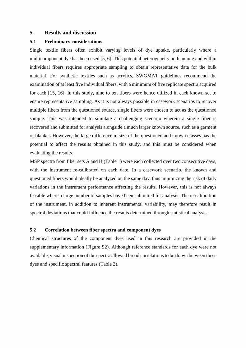
5.3 Distribution of the spectral dataset PCA revealed that 96.6 % of total variance in the dataset could be described by the first three

PCs, as illustrated in the scree plot below (Figure 2). The scree plot is important in determining

the optimum number of PCs to be retained within the model [29]. Retaining an insufficient

number of PCs may cause information pertaining to dataset variation being lost, whilst

extraneous PCs may result in the modelling of random variance or noise [29, 49]. By assessing

the variance accounted for by each individual PC, and determining the point at which the curve

begins to plateau, the optimum number of PCs required to model the data can be identified [32,

50]. In this case, the scree plot indicated that the use of up to four PCs (accounting for 98.5 %

of the total variation) was suitable to re-visualize the dataset.

Figure 2: Scree plot depicting the cumulative variance in the dataset retained by each PC.

Scores plots generated using combinations of the first four PCs resulted in most fiber sets

forming visually distinct clusters, with no obvious outliers (Figure 3). PC4, despite accounting

for only 1.9 % of variance within the dataset, was found to improve the discrimination between

fiber sets C and D. These exemplars were observed to overlap when utilizing only the first

three PCs. Fiber sets A and H exhibited significant overlap, which was attributed to these fibers

possessing the same dye combination (Table 1). It should also be noted, though, that these

fibers have different diameters, and would hence be distinguishable based upon a general

microscopic examination.

Spectra from sets D and E exhibited a high level of spread (i.e. intra-class variance) compared

to the remaining samples when employing the first three PCs. Visual inspection of the

corresponding spectra (Figure S3) revealed variation in the relative absorbance between bands

in the 400-500 nm (yellow dye) region and those in the 600 nm (blue dye) region. This is

potentially due to differing dye uptake amongst individual fibers, as discussed above. This also

reinforces the importance of collecting an adequate number of fibers and replicate spectra to

allow representative measurements to be obtained.

Figure 3: 3-dimensional PCA scores plot (employing PCs 1,2,3 and PCs 1,2,4) showing the distribution

of blue acrylic fibers based upon their corresponding MSP spectra. Left and right images show the

improved separation of Fiber Sets C and D upon the inclusion of PC4.

The factor loadings for the first four PCs (Figure 4) can be used to identify which wavelength

regions are the largest contributors to variation between the fiber sets, and consequently

between each Q vs. K pair. PC1 has a strong positive correlation at ca. 655 nm, consistent with

the absorbance band for Blue 3 dye. Samples separated along this PC may therefore be assumed

to differ in their relative proportions of this dye. For example, fibers from set F (containing

Blue 3) attain positive scores against PC1, while fibers from set E (instead containing Blue

147) exhibit negative scores. Similarly, PC2 has a positive correlation at 450 nm, consistent

with Yellow 28 dye. Fiber pairs separated along this component are hence assumed to be

dissimilar in terms of the type or concentration of yellow dye present.

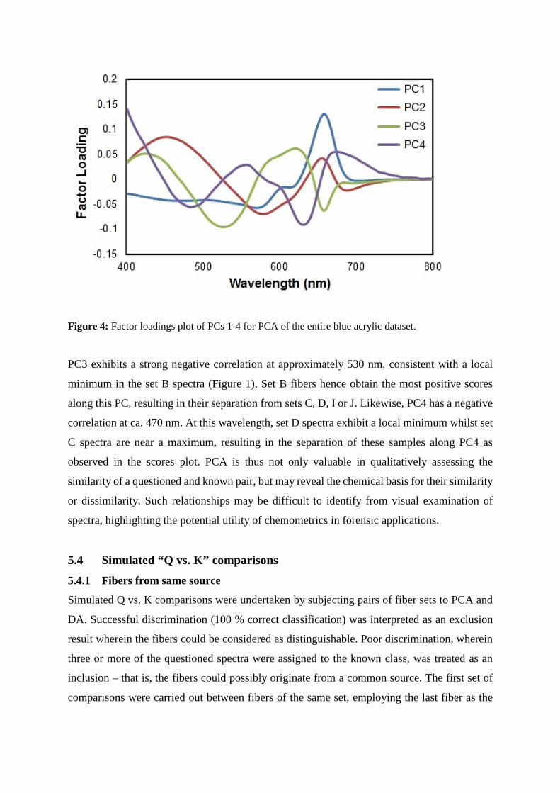
Figure 4: Factor loadings plot of PCs 1-4 for PCA of the entire blue acrylic dataset.

PC3 exhibits a strong negative correlation at approximately 530 nm, consistent with a local

minimum in the set B spectra (Figure 1). Set B fibers hence obtain the most positive scores

along this PC, resulting in their separation from sets C, D, I or J. Likewise, PC4 has a negative

correlation at ca. 470 nm. At this wavelength, set D spectra exhibit a local minimum whilst set

C spectra are near a maximum, resulting in the separation of these samples along PC4 as

observed in the scores plot. PCA is thus not only valuable in qualitatively assessing the

similarity of a questioned and known pair, but may reveal the chemical basis for their similarity

or dissimilarity. Such relationships may be difficult to identify from visual examination of

spectra, highlighting the potential utility of chemometrics in forensic applications.

5.4 Simulated “Q vs. K” comparisons 5.4.1 Fibers from same source

Simulated Q vs. K comparisons were undertaken by subjecting pairs of fiber sets to PCA and

DA. Successful discrimination (100 % correct classification) was interpreted as an exclusion

result wherein the fibers could be considered as distinguishable. Poor discrimination, wherein

three or more of the questioned spectra were assigned to the known class, was treated as an

inclusion – that is, the fibers could possibly originate from a common source. The first set of

comparisons were carried out between fibers of the same set, employing the last fiber as the

questioned sample and the remaining nine fibers as the known sample. These spectra were

expected to be non-differentiable, thus yielding an inclusion result.

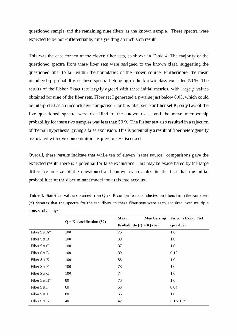
This was the case for ten of the eleven fiber sets, as shown in Table 4. The majority of the

questioned spectra from these fiber sets were assigned to the known class, suggesting the

questioned fiber to fall within the boundaries of the known source. Furthermore, the mean

membership probability of these spectra belonging to the known class exceeded 50 %. The

results of the Fisher Exact test largely agreed with these initial metrics, with large p-values

obtained for nine of the fiber sets. Fiber set I generated a p-value just below 0.05, which could

be interpreted as an inconclusive comparison for this fiber set. For fiber set K, only two of the

five questioned spectra were classified to the known class, and the mean membership

probability for these two samples was less than 50 %. The Fisher test also resulted in a rejection

of the null hypothesis, giving a false exclusion. This is potentially a result of fiber heterogeneity

associated with dye concentration, as previously discussed.

Overall, these results indicate that while ten of eleven “same source” comparisons gave the

expected result, there is a potential for false exclusions. This may be exacerbated by the large

difference in size of the questioned and known classes, despite the fact that the initial

probabilities of the discriminant model took this into account.

Table 4: Statistical values obtained from Q vs. K comparisons conducted on fibers from the same set.

(*) denotes that the spectra for the ten fibers in these fiber sets were each acquired over multiple

consecutive days

Q = K classification (%) Mean Membership

Probability (Q = K) (%)

Fisher’s Exact Test

(p-value)

Fiber Set A* 100 76 1.0

Fiber Set B 100 89 1.0

Fiber Set C 100 87 1.0

Fiber Set D 100 80 0.18

Fiber Set E 100 88 1.0

Fiber Set F 100 78 1.0

Fiber Set G 100 74 1.0

Fiber Set H* 80 78 1.0

Fiber Set I 60 53 0.04

Fiber Set J 80 66 1.0

Fiber Set K 40 42 5.1 x 10-4

5.4.2 Fibers from different sources

When comparing fibers originating from different sets, the majority of samples (with exception

of sets A vs. H and C vs. D) were unambiguously differentiated, yielding true exclusions in

108 of 110 comparisons. In these comparisons, 100 % correct classification was achieved and

the membership probability of the questioned spectra belonging to the known class was

determined to be 0 %. Successful discrimination of these fiber sets was expected based on their

clear visual separation in the PCA scores plot. As these samples could be readily differentiated

according to their PC scores, Fisher’s test was deemed unnecessary and is not included here.

When fiber sets C and D were compared, there was a small probability for some of the

questioned samples to be assigned to the known class (Table 5). This is consistent with the

minor overlap noted between these sample sets in the PCA scores plot when employing the

first three PCs. Nonetheless, as the probability associated with misclassification of the

questioned spectra was minimal (below 5 % in each case), the samples were still considered to

be separable. Fisher’s test also indicated that the Q vs. K membership frequencies for these

samples were interdependent, yielding an overall exclusion result.

Table 5: Statistical values obtained from Q vs. K comparisons on fibers from different sets.

Questioned Known Q = K

classification (%)

Mean

Membership

Probability

(Q = K) (%)

Fisher’s Exact

Test (p-value)

Fiber Set C Fiber Set D 0 3 4.7 x 10-7

Fiber Set D Fiber Set C 0 2 2.8 x 10-6

Fiber Set A Fiber Set H 60 47 8.2 x 10-3

Fiber Set H Fiber Set A 100 81 1.0

When comparing fiber sets A and H, the results were less conclusive. When a fiber from set A

made up the questioned sample, the majority (60 %) of these spectra were assigned to the

known class, although the mean membership probability was less than 50 %. Furthermore,

Fisher’s Exact test indicated that the two samples were distinguishable (p < 0.001). However,

when a fiber from set H made up the questioned sample, all questioned spectra were assigned

to the known class with high probability and Fisher’s Exact Test indicated that the two samples

were indistinguishable. Taken together, this indicates that fiber sets A and H were not able to

be reliably differentiated.

The inability to discriminate between these sets was expected given their high degree of overlap

in the PCA scores plot (Figure 3) and shared dye combination, although the relative

concentrations of each dye component were not determined. Additionally, though the diameters

of the fibers differed, normalization of the spectra was expected to nullify this difference.

Interestingly, visual examination of the spectra from sets A and H revealed varying ratios of

absorbance at the 655 nm peak and 650 nm shoulder (Figure S4). Both of these bands have

been attributed to the same dye (Blue 3), and so heterogeneous dye uptake would not appear to

be a contributing factor to this variation. As the spectra of these fiber sets were collected over

consecutive days, it is likely that these deviations are a result of systematic instrumental

variation or re-calibration, as discussed in section 5.1. For future studies, it would thus be more

appropriate to collect data for these fiber sets in a single session, rather than analyzing the fiber

sets sequentially over a number of days. Additionally, it should be noted in casework

examinations where data has been acquired over multiple days, as this may similarly affect

fiber examinations based upon visual data inspections.

6. Conclusions The use of statistical methods with MSP shows great potential for rapidly distinguishing

visually similar fibers on the basis of their dye combinations. The comparison of simulated

questioned and known fibers from the same source resulted in a correct inclusion result for nine

of the eleven fiber sets, although a false exclusion was obtained for fiber set K, and fiber set I

gave potentially ambiguous results. The comparison of questioned and known fibers from

different sources allowed for the differentiation of all fiber sets with the exception of fiber set

A and H, which shared the same dye combination, yielding true exclusion results in 108 of 110

comparisons.

The single false exclusion was attributed to a lack of reproducibility in obtaining the MSP

spectra. Spectra from several fiber sets (A, D, E and H) were also found to exhibit varying

absorbance ratios between particular peaks. This may result from the heterogeneous uptake of

multi-component dye mixtures by individual fibers. Alternatively, the analysis of samples

across different dates could result in spectral deviations due to instrumental variability or the

re-calibration of the instrument. Given the impact of these factors on the results obtained

through statistical analyses, it can be concluded that these methods are not infallible.

Nevertheless, the use of well-documented statistical protocols for these comparisons provides

a more scientifically rigorous basis on which examiners can support their findings in court.

As this study employed a limited sample range, additional work is required to determine

whether similar results can be obtained with other fiber or dye types. In particular, natural fibers

such as cotton or wool are of interest due to their common use in modern textiles. The greater

amount of natural variation amongst these fibers will also provide a more rigorous test of the

protocols employed in this study. Finally, it should be noted that the exemplars utilized in this

research were relatively new, and do not take into account potential effects due to laundering,

every day wear, or similar factors which real samples may be subjected to. Studies

incorporating such datasets will therefore be imperative for model validation, and to assess

whether such models may be reliably applied to real scenarios.

7. Acknowledgements The authors thank Dr. Stephen L. Morgan (University of South Carolina) for the provision of

samples for this study, as well as Dana Bors, Wil Kranz, and Maria Diez (IUPUI) for their

assistance in spectra acquisition.

Funding: Portions of this research were supported by the National Institute of Justice, Office

of Justice Programs [award number 2010-DN-BX-K220] . Georgina Sauzier was supported by

an Australian Postgraduate Award.

8. References

1. Brandl, S.G., Criminal Investigation. 2nd ed. 2007, Upper Saddle River, NJ: Prentice Hall. 2. Houck, M.M. and J.A. Siegel, Fundamentals of Forensic Science. 2nd ed. 2010, Burlington,

MA: Academic Press. 3. Robertson, J. and C. Roux, Fibers: Overview, in Encyclopedia of Forensic Sciences, J.A. Siegel

and P.J. Saukko, Editors. 2013, Academic Press: Waltham. p. 109-112. 4. Apsell, P., What are Dyes? What is Dyeing?, in Dyeing Primer, J.R. Aspland, Editor. 1981,

American Association of Textile Chemists and Colorists: Research Triangle Park, NC. p. 4-7. 5. Houck, M., Textiles, in Forensic Chemistry: Fundamentals and Applications, J.A. Siegel, Editor.

2016, Wiley-Blackwell: Chichester, UK. p. 40-74. 6. Palmer, R., Fibers: Identification and Comparison, in Encyclopedia of Forensic Sciences, J.A.

Siegel and P.J. Saukko, Editors. 2013, Academic Press: Waltham. p. 129-137. 7. Siegel, J.A., Forensic Science: The Basics. 2007, Boca Raton, Florida: Taylor & Francis. 8. Goodpaster, J.V. and E.A. Liszewski, Forensic analysis of dyed textile fibers. Analytical and

Bioanalytical Chemistry, 2009. 394(8): p. 2009-2018. 9. Martin, P., Fibers: Color Analysis, in Encyclopedia of Forensic Sciences, J.A. Siegel and P.J.

Saukko, Editors. 2013, Academic Press: Waltham. p. 148-154. 10. Eng, M., P. Martin, and C. Bhagwandin, The analysis of metameric blue fibers and their

forensic significance. Journal of Forensic Sciences, 2009. 54(4): p. 841-845. 11. Eyring, M.B. and B.D. Gaudette, An Introduction to the Forensic Aspects of Textile Fiber

Examination, in Forensic Science Handbook, R. Saferstein, Editor. 2005, Prentice Hall: Englewood Cliffs, NJ. p. 231-296.

12. Grieve, M.C., T. Biermann, and M. Davignon, The occurrence and individuality of orange and green cotton fibres. Science & Justice, 2003. 43(1): p. 5-22.

13. Marcrae, R., R.J. Dudley, and K.W. Smalldon, The characterization of dyestuffs on wool fibers with special reference to microspectrophotometry. Journal of Forensic Sciences, 1979. 24(1): p. 117-129.

14. Suzuki, S., et al., Microspectrophotometric discrimination of single fibres dyed by indigo and its derivatives using ultraviolet-visible transmittance spectra. Science & Justice, 2001. 41(2): p. 107-111.

15. Scientific Working Group on Materials Analysis, Forensic Fiber Examination Guidelines. 1999. 16. Scientific Working Group on Materials Analysis, Ultraviolet-Visible Spectroscopy of Textile

Fibers. 2011. 17. National Academy of Sciences, Strengthening Forensic Science in the United States: A Path

Forward. 2009, Committee on Identifying the Needs of the Forensic Sciences Community, National Research Council: Washington DC.

18. Causin, V., et al., Forensic analysis of acrylic fibers by pyrolysis–gas chromatography/mass spectrometry. Journal of Analytical and Applied Pyrolysis, 2006. 75(1): p. 43-48.

19. Gilbert, C. and S. Kokot, Discrimination of cellulosic fabrics by diffuse reflectance infrared Fourier transform spectroscopy and chemometrics. Vibrational Spectroscopy, 1995. 9(2): p. 161-167.

20. Ruckebusch, C., et al., Quantitative analysis of cotton-polyester textile blends from near-infrared spectra. Applied Spectroscopy, 2006. 60(5): p. 539-544.

21. Daéid, N.N., W. Meier-Augenstein, and H.F. Kemp, Investigating the provenance of un-dyed spun cotton fibre using multi-isotope profiles and chemometric analysis. Rapid Communications in Mass Spectrometry, 2011. 25(13): p. 1812-1816.

22. Fortier, C. and J. Rodgers, Preliminary examinations for the identification of U.S. domestic and international cotton fibers by near-infrared spectroscopy. Fibers, 2014. 2(4): p. 264-274.

23. Liu, Y., Vibrational spectroscopic investigation of Australian cotton cellulose fibres: Part 1 - A Fourier transform Raman study. Analyst, 1998. 123(4): p. 633-636.

24. Morgan, S.L., et al. Pattern recognition methods for the classification of trace evidence textile fibers from UV/visible and fluorescence spectra. in 2007 Trace Evidence Symposium. 2007. Clearwater Beach, Florida.

25. Kramer, R., Chemometric Techniques for Quantitative Analysis. 1998, New York: Marcel Dekker, Inc.

26. Girod, A. and C. Weyermann, Lipid composition of fingermark residue and donor classification using GC/MS. Forensic Science International, 2014. 238: p. 68-82.

27. Croxton, R.S., et al., Variation in amino acid and lipid composition of latent fingerprints. Forensic Science International, 2010. 199(1-3): p. 93-102.

28. Miller, J.N. and J.C. Miller, Statistics and Chemometrics for Analytical Chemistry. 6th ed. 2010, Harlow: Prentice Hall.

29. Otto, M., Chemometrics: Statistics and computer application in analytical chemistry. 2nd ed. 2007, Weinheim, Germany: Wiley-VCH.

30. Gemperline, P.J., Principal Component Analysis, in Practical Guide to Chemometrics. 2006, CRC Press: Boca Raton, Florida. p. 69-104.

31. Morgan, S.L. and E.G. Bartick, Discrimination of Forensic Analytical Chemical Data using Multivariate Statistics, in Forensic Analysis on the Cutting Edge: New Methods for Trace Evidence Analysis, R.D. Blackledge, Editor. 2007, John Wiley & Sons: New Jersey. p. 333-374.

32. Varmuza, K. and P. Filzmoser, Principal Component Analysis, in Introduction to Multivariate Statistical Analysis in Chemometrics. 2009, Taylor & Francis: Boca Raton, Florida.

33. Lavine Barry, K. and J. Workman, Chemometrics: Past, Present, and Future, in Chemometrics and Chemoinformatics. 2005, American Chemical Society. p. 1-13.

34. Kinton, V., Multivariate Techniques, in Practical Analysis of Flavor and Fragrance Materials. 2011, John Wiley & Sons. p. 91-110.

35. Bensmail, H. and G. Celeux, Regularized gaussian discriminant analysis through eigenvalue decomposition. Journal of the American Statistical Association, 1996. 91(436): p. 1743-1748.

36. Zadora, G., Chemometrics and Statistical Considerations in Forensic Science, in Encyclopedia of Analytical Chemistry, R.A. Meyers, Editor. 2006, John Wiley & Sons: New Jersey.

37. Mendlein, A., C. Szkudlarek, and J.V. Goodpaster, Chemometrics, in Encyclopedia of Forensic Sciences, J.A. Siegel and P.J. Saukko, Editors. 2013, Academic Press: Waltham. p. 646-651.

38. Brereton, R.G., Chemometrics: Data Analysis for the Laboratory and Chemical Plant. 2003, London: John Wiley & Sons.

39. Scientific Working Group on Materials Analysis, Introduction to Forensic Fiber Examination. 2011.

40. Fisher, R.A., Statistical Methods for Research Workers. 13th ed. 1958, Edinburgh: Oliver and Boyd.

41. Fisher, R.A., On the interpretation of χ2 from contingency tables, and the calculation of P. Journal of the Royal Statistical Society, 1922. 85(1): p. 87-94.

42. Fisher, R.A., The Design of Experiments. 8th ed. 1971, New York: Hafner Publishing Company. 43. Mao, J., et al., Removal of Basic Blue 3 from aqueous solution by Corynebacterium

glutamicumbiomass: Biosorption and precipitation mechanisms. Korean Journal of Chemical Engineering, 2008. 25(5): p. 1060-1064.

44. Sigma Aldrich. Basic Blue 3. 2015; Available from: http://www.sigmaaldrich.com/catalog/product/aldrich/378011?lang=en&region=AU.

45. Wawrzkiewicz, M., Removal of C.I. Basic Blue 3 dye by sorption onto cation exchange resin, functionalized and non-functionalized polymeric sorbents from aqueous solutions and wastewaters. Chemical Engineering Journal, 2013. 217: p. 414-425.

46. Ceron-Rivera, M., M.M. Davila-Jimenez, and M.P. Elizalde-Gonzalez, Degradation of the textile dyes Basic yellow 28 and Reactive black 5 using diamond and metal alloys electrodes. Chemosphere, 2004. 55: p. 1-10.

47. Iranifam, M., M. Zarei, and A.R. Khataee, Decolorization of C.I. Basic Yellow 28 solution using supported ZnO nanoparticles coupled with photoelectro-Fenton process. Journal of Electroanalytical Chemistry, 2011. 659(1): p. 107-112.

48. Speers, S.J., B.H. Little, and M. Roy, Separation of acid, basic and dispersed dyes by a single-gradient elution reversed-phase high-performance liquid chromatography system. Journal of Chromatography A, 1994. 674(1-2): p. 263-70.

49. Brereton, R.G., Pattern Recognition, in Applied Chemometrics for Scientists. 2007, John Wiley & Sons: Chichester, England. p. 145-191.

50. Adams, M.J., Chemometrics in Analytical Spectroscopy. 2nd ed. 2004, Cambridge: Royal Society of Chemistry.