Improving the Accuracy of Top-N Recommendation …pike.psu.edu/publications/is16-PrefCF.pdfImproving...

Improving the Accuracy of Top-N Recommendationusing a Preference ModelI

Jongwuk Leea, Dongwon Leeb,, Yeon-Chang Leec, Won-Seok Hwangc,Sang-Wook Kimc

aHankuk University of Foreign Studies, Republic of KoreabThe Pennsylvania State University, PA, USA

cHanyang University, Republic of Korea

Abstract

In this paper, we study the problem of retrieving a ranked list of top-N items to atarget user in recommender systems. We first develop a novel preference modelby distinguishing different rating patterns of users, and then apply it to existingcollaborative filtering (CF) algorithms. Our preference model, which is inspiredby a voting method, is well-suited for representing qualitative user preferences. Inparticular, it can be easily implemented with less than 100 lines of codes on top ofexisting CF algorithms such as user-based, item-based, and matrix-factorization-based algorithms. When our preference model is combined to three kinds of CFalgorithms, experimental results demonstrate that the preference model can im-prove the accuracy of all existing CF algorithms such as ATOP and NDCG@25by 3%–24% and 6%–98%, respectively.

1. Introduction

The goal of recommender systems (RS) [1] is to suggest appealing items (e.g.,movies, books, news, and music) to a target user by analyzing her prior prefer-

IThis work was supported by Hankuk University of Foreign Studies Research Fund of 2014(Jongwuk Lee). His research was in part supported by NSF CNS-1422215 and Samsung 2015GRO-175998 awards (Dongwon Lee). This work was partly supported by the National Re-search Foundation of Korea (NRF) grant funded by the Korean Government (MSIP) (NRF-2014R1A2A1A10054151) and by the Ministry of Science, ICT and Future Planning (MSIP),Korea, under the Information Technology Research Center (ITRC) support program (IITP-2015-H8501-15-1013) (Sang-Wook Kim).

Email addresses: [email protected] (Jongwuk Lee), [email protected] (DongwonLee), [email protected] (Yeon-Chang Lee),[email protected] (Won-Seok Hwang), [email protected](Sang-Wook Kim)

Preprint submitted to Elsevier February 7, 2016

1 2 3 4 50

1

2

3

4

5

Item id

Rat

ing

1 2 3 4 50

1

2

3

4

5

Item id

Rat

ing

(a) user u (b) user v

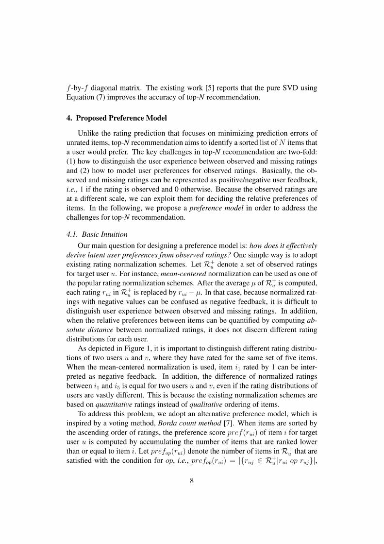
Figure 1: The rating distribution of two users u and v

ences. As the number of applications using RS as a core component has increasedrapidly, improving the quality of RS becomes a critically important problem. Thequality of RS can be measured by various criteria such as accuracy, serendip-ity, diversity, relevance, and utility [29, 38]. In measuring the accuracy of RS,in particular, two approaches have prevailed: rating prediction and top-N recom-mendation [36]. A typical practice of rating prediction is to minimize predictionerrors for all unobserved (or missing) user-item pairs. In contrast, top-N recom-mendation provides users with the most appealing top-N items. In this paper, wemainly focus on improving the accuracy of top-N recommendation.

Collaborative filtering (CF) [37] has been widely used as one of the mostpopular techniques in RS. Basically, it is based on users’ past behavior such asexplicit user ratings and implicit click logs. Using the similarity between users’behavior patterns, CF suggests the most appealing top-N items for each user. Inthis process, existing CF algorithms [6, 10, 11, 16, 30, 31] return top-N items withthe highest ratings in terms of rating prediction, and ignore the qualitative orderof items for top-N recommendation. Although some recent work [2, 5, 20, 32, 39]developed CF algorithms for optimizing top-N recommendation, they still havethe limitations in identifying qualitative user preferences, i.e., relative preferencesbetween items with explicit ratings.

Specifically, two key issues in existing top-N recommendation are: (1) howto distinguish user experience between observed and missing ratings and (2) howto model latent user preferences from observed ratings. As the solution to (1),for instance, we may impute missing ratings as zero (i.e., negative user feedback),as used in [5]. However, as to the solution to (2), it is non-trivial to distinguishrelative preferences between observed ratings (i.e., positive user feedback) as userratings often have different distributions per user.

To motivate our preference model, we illustrate a scenario in which two usersu and v have rated for the same set of five items {i1, . . . , i5} (Figure 1). Even if

2

two users gave the same rating of 5 to item i5, the meaning of the rating can beinterpreted differently depending on rating distributions. For example, supposethat both u and v gave 5 to i5. Because v tends to give many ratings of 5, it isdifficult to determine how satisfactory v was really with i5. In contrast, because urarely gives the rating of 5, it is plausible to assure that u is very satisfied with i5.Therefore, we argue that u prefers i5 more than v does.

Our proposed preference model, which is inspired by a voting method, aims todiscern subtle latent user preferences by considering different rating distributions.While existing algorithms are mainly based on the quantitative values amongitems to represent user preferences, our model exploits the qualitative order ofitems. Our preference model is able to convert raw user ratings into latent userpreferences. In our formal analysis, it can be derived from maximum likelihoodestimation, which is consistent with existing work [14].

We then develop a family of CF algorithms by embedding the proposed pref-erence model into existing CF algorithms. As an orthogonal way, our prefer-ence model can be easily combined with existing CF algorithms such as user-based neighborhood, item-based neighborhood, and matrix-factorization-basedalgorithms. Observed user ratings are converted to user preference scores andmissing ratings are imputed as zero values. After this conversion is performed,existing CF algorithms are applied with the converted user-item matrix. The keyadvantages of our proposed algorithms are two-fold: a simple algorithm designand a sizable accuracy improvement in various kinds of CF algorithms.

In order to validate our proposed algorithms, we lastly conduct comprehensiveexperiments with extensive settings. Because user ratings tend to be biased to itempopularity and rating positivity [5, 27, 35], we employ two testing item sets: AllItems (i.e., all items in a test item set) and Long-tail Items (i.e., non-popular itemswith a few ratings) [5]. In case of cold-start users [21] who have rated only a fewitems, we also compare our proposed algorithms against existing CF algorithms.

To summarize, this paper makes the following contributions.

• We design a preference model in order to identify latent user preferencesfrom user ratings. The idea of the preference model is intuitive to under-stand, and easy to implement, costing less than 100 lines of codes, on topof existing CF algorithms.

• We propose a family of CF algorithms by incorporating the proposed pref-erence model into existing CF algorithms. Our preference model can beeasily applied to existing CF algorithms.

• We evaluate our proposed CF algorithms applied to user-based, item-based,and matrix-factorization-based algorithms. Our proposed algorithms arevalidated over two test sets: All Items and Long-tail Items. It is found that

3

our proposed algorithms improve three kinds of CF algorithms by 3%–24%and 6%–98% for ATOP and NDCG@25.

This paper is organized as follows. In Section 2, we survey existing work fortop-N recommendation. In Section 3, we discuss two categories of CF algorithmsand their variants for top-N recommendation. In Section 4, we design a preferencemodel and propose a family of CF algorithms using our preference model. InSection 5, we show detailed evaluation methodology. In Section 6, we report andanalyze the experimental results of our proposed algorithms. In Section 7, wefinally conclude our work.

2. Related Work

Collaborative filtering (CF) [37] is well-known as one of the most prevalenttechniques in recommender systems (RS). (The broad survey for RS can be foundin [1, 29].) Conceptually, it collects the past behavior of users, and makes ratingpredictions based on the similarity between users’ behavior patterns. The under-lying assumptions behind CF are as follows: (1) If users have similar behaviorpatterns in the past, they will also make similar behavior patterns in the future. (2)The users’ behavior patterns are consistent over time. The user behavior is usedto infer hidden user preferences and is usually represented by explicit (e.g., userratings) and implicit user actions (e.g., clicks and query logs). In this paper, weassume that the user behavior is represented by explicit user ratings on items.

The approaches for CF can be categorized as two models: neighborhood mod-els and latent factor models [37]. First, the neighborhood models make predictionsbased on the similarity between users or items such as user-based algorithms [10]and item-based algorithms [31]. Second, the latent factor models learn hiddenpatterns from observed ratings by using matrix factorization techniques [11, 17].In particular, singular value decomposition (SVD) is widely used as one of thewell-established techniques [13, 15, 16, 30]. In this paper, we mainly handle CFalgorithms with explicit user ratings.

Evaluation of top-N recommendation: Top-N recommendation provides userswith a ranked set of N items [6], which is also involved to the “who rated what”problem [4]. To evaluate top-N recommendation, we have to take the charac-teristics of observed ratings into account. That is, ratings are distributed not atrandom [22, 23, 34]. The ratings are biased to item popularity [5, 35] and tend tobe more preferred than missing ratings, i.e., rating positivity [27]. In this paper,we thus employ two testing items such as All Items and Long-tail Items, and adoptvarious metrics for fair evaluation of top-N recommendation.

One-class collaborative filtering: When user ratings are represented by binaryvalues, observed user ratings are simply set as one (positive feedback). Mean-

4

while, because missing ratings can be seen as a mixture of unknown and negativefeedback, they need to be considered carefully. First, [26] introduced this problemto distinguish different semantics of missing ratings. In addition, [25] proposedan improved weight scheme to discern missing ratings. As the simplest way, weimputed all missing ratings as zero (i.e., negative feedback). We compare our pro-posed algorithms with the one class collaborative filtering method, where miss-ing values are considered negative feedback with uniform weights. In our futurework, we will discuss an alternative method for handling missing ratings, e.g., aimputation method [21] for missing ratings.

Ranking-oriented collaborative filtering: For top-N recommendation, it is im-portant to consider the ranking of items. Weimer et al. [39] proposed CoFi-Rank that uses maximum margin matrix factorization to optimize the rankingof items. Liu et al. [20] developed EigenRank to decide the rankings of itemsusing neighborhood-based methods and Hu [12] proposed a preference-relation-based similarity measure for multi-criteria dimensions. In addition, [2, 32] com-bined CF with learning to rank methods to optimize the ranking of items. Shi etal. [33] combined rating- and ranking-oriented algorithms with a linear combina-tion function, and Lue et al. [19] extended probabilistic matrix factorization withlist-wise preferences. Rendle et al. [28] proposed Bayesian personalized rankingthat maximizes the likelihood of pair-wise preferences between observed and un-observed items in implicit datasets. In particular, [28] proposed a new objectivefunction that aims to achieve higher accuracy for top-N recommendation. Ningand Karypis [24] developed a sparse linear method that learns a coefficient matrixof item similarity for top-N recommendation. Recently, [38] developed a hybridapproach to combining the content-based the and collaborative filtering method inwhich the user participates in the feedback process by ranking her interests in theuser profiles. Liu et al. [18] adopted boosted regression trees to represent condi-tional user preferences in CF algorithms. In this paper, we propose an alternativeuser preference model, and combine it with a family of CF algorithms.

3. Collaborative Filtering Algorithms

In this section, we first introduce basic notations used throughout this paper.The domain consists of a set of m users, U = {u1, . . . , um}, and a set of n items,I = {i1, . . . , in}. All user-item pairs can be represented by an m-by-n matrixR = U × I, where an entry rui indicates the rating of user u to item i. If ruihas been observed (or known), it is represented by a positive value in a specificrange. Otherwise, rui is empty, implying a missing (or unknown) rating. LetR+ ⊆ R denote a subset of user-item pairs for which ratings are observed, i.e.,R+ = {rui ∈ R|rui is observed}. For the sake of representation, u and v indicatearbitrary users in U , and i and j refer to arbitrary items in I.

5

In the following, we explain existing CF algorithms. They can be categorizedinto: (1) neighborhood-based models and (2) latent-factor-based models.

3.1. Neighborhood ModelsThe neighborhood models are based on the similarity between either users or

items. There are two major neighborhood algorithms, i.e., user-based and item-based algorithms, depending on which sides are used. The user-based algorithmsmake predictions based on users’ rating patterns similar to that of a target user u.Let U(u; i) be a set of users who rate item i and have similar rating patterns to thetarget user u. The predicted rating rui of user u to item i is computed by:

rui = bui +

∑v∈U(u;i) (rvi − bvi)wuv∑

v∈U(u;i)wuv(1)

where rvi is a rating of user v to item i, bvi is a biased rating value for v to i, andwuv is the similarity weight between two users u and v. In other words, rui iscalculated by a weighted combination of neighbors’ residual ratings. Note that buiand wuv can be different depending on the rating normalization scheme and thesimilarity weight function.

On the other hand, the item-based algorithms predict the rating for target itemi of user u based on the rating patterns between items. Let I(i;u) be a set of itemsthat have rating patterns similar to that of i and have been rated by u. Let wijdenote the similarity weight between two items i and j. Specifically, the predictedrating rui is calculated by:

rui = bui +

∑j∈I(i;u) (ruj − buj)wij∑

j∈I(i;u)wij(2)

We discuss how the neighborhood models can be adapted for top-N recom-mendation. It is observed that predicting the exact rating values is unnecessaryfor top-N recommendation. Instead, it is more important to distinguish the impor-tance of items that are likely to be appealing to the target user. Toward this goal,items are ranked by ignoring the denominator used for rating normalization. Bysimply removing the denominators in Equations (1) and (2), it can only considerthe magnitude of observed ratings. This modification can help discern the userexperience between observed and missing ratings. Formally, the predicted scoreis computed by:

rui = bui +∑

v∈U(u;i)

(rvi − bvi)wuv (3)

Similarly, the predicted score in the item-based algorithms is calculated by:

rui = bui +∑

j∈I(i;u)

(ruj − buj)wij (4)

6

Note that rui in Equations (3) and (4) means the score for quantifying the im-portance of item i to user u. For top-N recommendation, it is observed thatthe non-normalized algorithms outperform conventional neighborhood algorithmsthat minimize prediction errors. The results are also consistently found in existingwork [5].

3.2. Latent Factor ModelsThe latent factor model is an alterative way to infer hidden characteristics of

rating patterns by using matrix factorization techniques. In this paper, we adoptsingular value decomposition (SVD) as the well-established matrix factorizationmethod [17]. A key idea of SVD is to factorize an m-by-n matrix R into aninner product of two low-rank matrices with dimension f . That is, one low-rankmatrix is called an m-by-f user-factor matrix and the other is called an n-by-fitem-factor matrix. Each user u is thus associated with an f -dimensional vectorpu ∈ Rf , and each item i is involved with an f -dimensional vector qi ∈ Rf .Formally, the predicted rating rui is calculated by:

rui = bui + puqTi (5)

In this process, a key challenge is how to handle the presence of missing rat-ings. Recent work adopts an objective function that only minimizes predictionerrors for observed ratings with regularization. Formally, the objective function isrepresented by:

minp,q,b

1

2

∑rui∈R+

(rui − bui − puqTi )2 +λ

2(||pu||2 + ||qi||2) (6)

where λ is a parameter for regularization. In order to improve the accuracy ofrating predictions, other information such as implicit user feedback [13] and tem-poral effects [15] can be used together in the objective function.

Although the objective function is effective for minimizing prediction errors,it does not obtain high accuracy for top-N recommendation [5]. This is becauseit does not differentiate between observed ratings and missing ratings. As a sim-plest way, all missing ratings are considered negative user feedback, and they areimputed as zero, i.e., ∀rui ∈ R/R+ : rui = 0. The imputation for missing ratingsenables us to discern user experience between observed ratings and missing rat-ings. Furthermore, because this modification can form a complete m-by-n matrixR, the conventional SVD method can be applied toR.

R ≈ UΣV T (7)

where a low-rank matrix approximation is used with dimension f . That is, U isan n-by-f orthonormal matrix, V is an m-by-f orthonormal matrix, and Σ is an

7

f -by-f diagonal matrix. The existing work [5] reports that the pure SVD usingEquation (7) improves the accuracy of top-N recommendation.

4. Proposed Preference Model

Unlike the rating prediction that focuses on minimizing prediction errors ofunrated items, top-N recommendation aims to identify a sorted list ofN items thata user would prefer. The key challenges in top-N recommendation are two-fold:(1) how to distinguish the user experience between observed and missing ratingsand (2) how to model user preferences for observed ratings. Basically, the ob-served and missing ratings can be represented as positive/negative user feedback,i.e., 1 if the rating is observed and 0 otherwise. Because the observed ratings areat a different scale, we can exploit them for deciding the relative preferences ofitems. In the following, we propose a preference model in order to address thechallenges for top-N recommendation.

4.1. Basic IntuitionOur main question for designing a preference model is: how does it effectively

derive latent user preferences from observed ratings? One simple way is to adoptexisting rating normalization schemes. Let R+

u denote a set of observed ratingsfor target user u. For instance, mean-centered normalization can be used as one ofthe popular rating normalization schemes. After the average µ ofR+

u is computed,each rating rui inR+

u is replaced by rui− µ. In that case, because normalized rat-ings with negative values can be confused as negative feedback, it is difficult todistinguish user experience between observed and missing ratings. In addition,when the relative preferences between items can be quantified by computing ab-solute distance between normalized ratings, it does not discern different ratingdistributions for each user.

As depicted in Figure 1, it is important to distinguish different rating distribu-tions of two users u and v, where they have rated for the same set of five items.When the mean-centered normalization is used, item i1 rated by 1 can be inter-preted as negative feedback. In addition, the difference of normalized ratingsbetween i1 and i5 is equal for two users u and v, even if the rating distributions ofusers are vastly different. This is because the existing normalization schemes arebased on quantitative ratings instead of qualitative ordering of items.

To address this problem, we adopt an alternative preference model, which isinspired by a voting method, Borda count method [7]. When items are sorted bythe ascending order of ratings, the preference score pref(rui) of item i for targetuser u is computed by accumulating the number of items that are ranked lowerthan or equal to item i. Let prefop(rui) denote the number of items inR+

u that aresatisfied with the condition for op, i.e., prefop(rui) = |{ruj ∈ R+

u |rui op ruj}|,

8

where op can be replaced with any comparison operator, e.g.,>,<, and =. Specif-ically, there are two cases for computing the preference score.

1. Given user rating rui, we simply count the number of items that are rankedlower than i. Let pref>(rui) is the preference score of rui, which is thenumber of items with lower rankings, i.e., pref>(rui) = |{ruj ∈ R+

u |rui >ruj}|.

2. Let pref=(rui) is the preference score of rui, which is the number of itemswith the same rankings, i.e., pref=(rui) = |{ruj ∈ R+

u |rui = ruj}|.

By combining the two cases, the preference score of rui can be computed as aweighted linear combination, where |R+

u | is used as a normalization parameter.

pref(rui) = α · pref>(rui)

|R+u |

+ β · pref=(rui)

|R+u |

(8)

where α and β are weight parameters for pref>(rui) and pref=(rui), respectively.Using this equation, we can convert user ratings into qualitative user preferencescores depending on different rating distributions.

We now explain how to compute the preference scores of items with cate-gories. When a set of user ratings is aggregated into a set of rating categories,it is easier to handle the set of rating categories with a smaller size, e.g., rui ∈{1, . . . , 5}. Let {C1, . . . , Ck} be a set of rating categories in a specific range. In-tuitively, the items in a high rating category are ranked higher than those in a lowrating category. Suppose that rui belongs to category C, i.e., rui ∈ C. To computethe preference score of rui, we simply count the number of items that are in lowrating category C ′, i.e., C > C ′, and the number of items in the same category C.The preference score pref(C) of C is computed as:

pref(C) = α ·∑

C′∈{C1,...Ck}

pref>(C,C ′)

|R+u |

+ β · pref=(C)

|R+u |

(9)

where pref>(C,C ′) is the number of items that belong to lower rating categoryC ′ and pref=(C) is the number of items that belong to C. Based on the formalanalysis in Section 4.3, parameters α and β are set as 1.0 and 0.5, respectively.

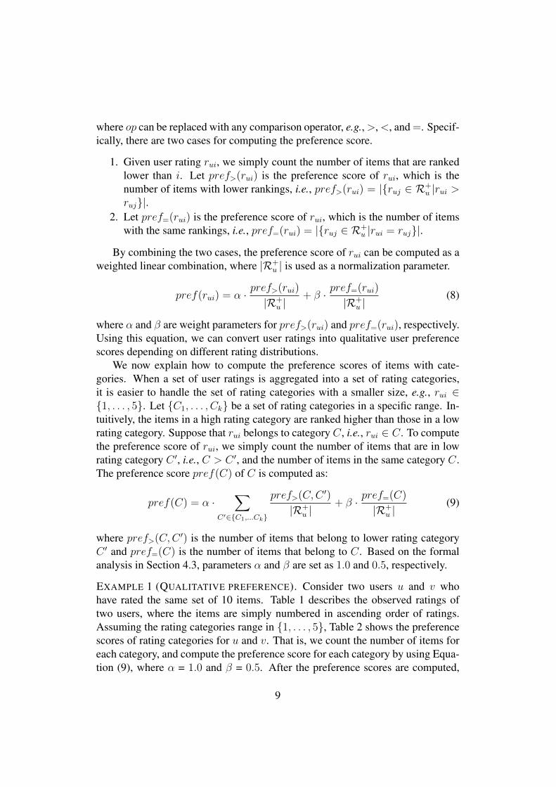
EXAMPLE 1 (QUALITATIVE PREFERENCE). Consider two users u and v whohave rated the same set of 10 items. Table 1 describes the observed ratings oftwo users, where the items are simply numbered in ascending order of ratings.Assuming the rating categories range in {1, . . . , 5}, Table 2 shows the preferencescores of rating categories for u and v. That is, we count the number of items foreach category, and compute the preference score for each category by using Equa-tion (9), where α = 1.0 and β = 0.5. After the preference scores are computed,

9

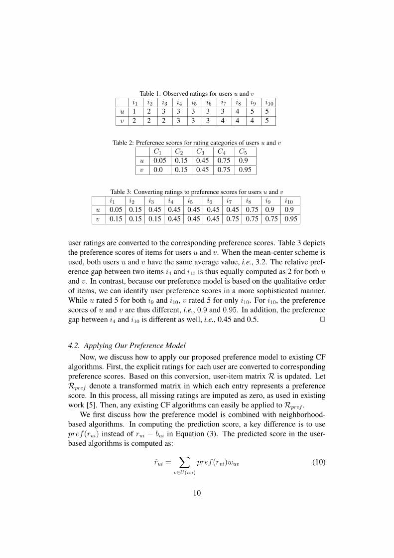
Table 1: Observed ratings for users u and v

i1 i2 i3 i4 i5 i6 i7 i8 i9 i10u 1 2 3 3 3 3 3 4 5 5v 2 2 2 3 3 3 4 4 4 5

Table 2: Preference scores for rating categories of users u and v

C1 C2 C3 C4 C5

u 0.05 0.15 0.45 0.75 0.9v 0.0 0.15 0.45 0.75 0.95

Table 3: Converting ratings to preference scores for users u and v

i1 i2 i3 i4 i5 i6 i7 i8 i9 i10u 0.05 0.15 0.45 0.45 0.45 0.45 0.45 0.75 0.9 0.9v 0.15 0.15 0.15 0.45 0.45 0.45 0.75 0.75 0.75 0.95

user ratings are converted to the corresponding preference scores. Table 3 depictsthe preference scores of items for users u and v. When the mean-center scheme isused, both users u and v have the same average value, i.e., 3.2. The relative pref-erence gap between two items i4 and i10 is thus equally computed as 2 for both uand v. In contrast, because our preference model is based on the qualitative orderof items, we can identify user preference scores in a more sophisticated manner.While u rated 5 for both i9 and i10, v rated 5 for only i10. For i10, the preferencescores of u and v are thus different, i.e., 0.9 and 0.95. In addition, the preferencegap between i4 and i10 is different as well, i.e., 0.45 and 0.5. 2

4.2. Applying Our Preference ModelNow, we discuss how to apply our proposed preference model to existing CF

algorithms. First, the explicit ratings for each user are converted to correspondingpreference scores. Based on this conversion, user-item matrix R is updated. LetRpref denote a transformed matrix in which each entry represents a preferencescore. In this process, all missing ratings are imputed as zero, as used in existingwork [5]. Then, any existing CF algorithms can easily be applied toRpref .

We first discuss how the preference model is combined with neighborhood-based algorithms. In computing the prediction score, a key difference is to usepref(rui) instead of rui − bui in Equation (3). The predicted score in the user-based algorithms is computed as:

rui =∑

v∈U(u;i)

pref(rvi)wuv (10)

10

Similarly, the predicted score in the item-based algorithms is calculated as:

rui =∑

j∈I(i;u)

pref(ruj)wij (11)

In both cases, rui indicates the importance of items for top-N recommendation.Next, we explain how to apply the preference model for latent factor based

algorithms. For top-N recommendation, ranking-based models (e.g., [39, 32, 2])employ an objective function that minimizes the error of item ranking. However,because the models are mainly based on the ordering of pair-wise items, theymay fail to reflect overall rating distributions. In addition, their computation over-head is prohibitevely high if all pair-wise preferences of items are considered. Toaddress this problem, we first transform R into Rpref (as done in neighborhood-based algorithms), and then factorizeRpref using the conventional SVD method.

Rpref ≈ UΣV T (12)

4.3. Formal AnalysisWe now derive the preference model by using maximum likelihood estimation.

For simplicity, suppose that a set of ratings is represented by a rating distributionwith categories. Given a set of category {C1, . . . , Ck}, Xi denotes a set of itemsassigned to the corresponding rating category Ci. All items with ratings are asso-ciated with {X1, . . . , Xk}. We estimate a preference score θi for the correspond-ing rating category Ci. Let θ = {θ1, . . . , θk} denote probability scores that eachcategory is preferred. When generating a ranked list L of observed items for userpreferences, we identify a parameter θ that maximizes the likelihood function.

θ∗ = arg maxθ

p(L|θ) (13)

In that case, p(L|θ) can be replaced by the product of probability of generatingthe correct ranked list for any two items. That is, p(L|θ) is represented by:

p(L|θ) =∏i>j

∏x∈Xi,x′∈Xj

p(x > x′|θ)

×∏i

( ∏x 6=x′∈Xi

p(x > x′|θ)

)(14)

where p(x > x′|θ) is the probability that item x is preferred to item x′, followingbinary distribution for p(x):

p(x > x′|θ) = p(x)(1− p(x′)) (15)

11

Table 4: Detailed statistics of real-life datasetsMovieLens 100K MovieLens 1M

Density 6.30% 4.26%Min. # of ratings of users 20 20Max. # of ratings of users 737 2,314Avg. # of ratings per user 106.04 165.59

where p(x) is the probability that item x is preferred.As discussed in Section 4.1, a set of user ratings is represented by a set of

discrete rating categories {C1, . . . , Ck}. We can replace p(X) with the probabilityp(Ci) for rating category Ci, and combine Equations (14) with (15). Therefore,p(L|θ) can be computed by:

p(L|θ) =∏Ci>Cj

(p(Ci)

n(Ci)(1− p(Cj))n(Cj))×

∏Ci

(p(Ci)(1− p(Ci)))n(Ci)(n(Ci)−1)/2 (16)

where n(Ci) is the number of items assigned to Ci.By maximizing the log likelihood of p(L|θ), we can finally obtain the highest

preference probability θi ∈ θ, which is derived as:

p(Ci) =∑i>j

p(Ci > Cj) +1

2× p(Ci = Cj) (17)

where p(Ci > Cj) is the probability that Ci is preferred to Cj , and p(Ci = Cj) isthe probability that Ci and Cj are preferred equally. In our experiments, we set α= 1.0 and β = 0.5 in Equation (9). It is found that the derivation for our preferencemodel is consistent with existing work [14].

5. Evaluation Methodology

In this section, we first explain real-life datasets used for evaluation (Sec-tion 5.1), and then show various accuracy metrics for top-N recommendation(Section 5.2).

5.1. DatasetsWe employ two real-life datasets of MovieLens 100K and MovieLens 1M.

These are publicly available at http://grouplens.org/datasets/movielens. The Movie-Lens 100K dataset includes 943 users, 1,682 items, and 100,000 ratings, and theMovieLens 1M dataset includes 6,040 users, 3,952 items, and 1,000,209 ratings.

12

200 400 600 800 1000 1200 1400 16000

100

200

300

400

500

Item id

# of

rat

ings

long−tail items

top−head items

Figure 2: The popularity distribution of items in MovieLens 100K

The ratings take integer values ranging from 1 (worst) to 5 (best). Table 4 sum-marizes the statistics for the two datasets.

For fair evaluation, we run a 5-fold cross validation. The dataset is randomlysplit into two subsets, i.e., 80% training and 20% testing data. Let Tr ⊂ R+

and Te ⊂ R+ denote training and testing subsets partitioned from R+, i.e., Tr ∩Te = ∅, Tr ∪ Te = R+. Each subset is used for executing and evaluating CFalgorithms. Specifically, Tru and Teu denote a set of items rated by target user u,i.e., Tru = {i ∈ I|rui ∈ Tr} and Teu = {i ∈ I|rui ∈ Te}. In particular, theitems with the highest ratings are taken as relevant items in Teu. Let Te+u denote aset of relevant items, i.e., Te+u = {i ∈ I|rui ∈ Teu, rui = 5}. That is, Te+u is usedas ground truth for measuring accuracy metrics. Meanwhile, the items with lowratings and unrated items are considered non-relevant. In other words, suggestingthe most preferred items only is treated as an effective top-N recommendation.

In order to evaluate top-N recommendation, it is also important to select a setof candidate items that CF algorithms will rank. Let Lu denote a set of candidateitems to be ranked for user u. Given Lu, the CF algorithms sort Lu by the de-scending order of prediction scores and generate a sorted list with top-N items.Depending on the selection of Lu, different top-N items can be created [3]. For ageneralized setting, we form Lu = I − Tru as a set of whole items except for theitems that have been rated by user u. In this paper, we call this setting All Items.

When using All Items, it is observed that the majority of ratings is biasedto only a small fraction of popular items. Figure 2 depicts the distribution ofitems in MovieLens 100K, where Y -axis represents popularity, i.e., the numberof observed ratings. The items in X-axis are sorted by the descending order ofpopularity. In Figure 2, the top-100 popular items (i.e., about 6%) have 29,931ratings (i.e., about 30%). In that case, because the top-N items tend to be biased toa few popular items, top-N recommendation may not bring much benefit for users.

13

Note that the popularity bias of rated items can be found in other datasets [5, 27].To address this problem, we design a more elaborated setting in selecting Lu.

Given a set I of items, it is partitioned into two subsets in terms of popularity.That is, most popular 100 items and remaining items are called top-head andlong-tail items, respectively. Let Top denote a set of top-head items. In that case,we deliberately form Lu as long-tail items, i.e., Lu = (I − Top)− Tru as shownin [5]. We call this setting Long-tail Items. The evaluation for long-tail items canbe less biased toward the popular items. Compared to All Items, it can be a moredifficult setting. For extensive evaluation, we will use both settings, i.e., All Itemsand Long-tail Items.

Lastly, we evaluate top-N recommendation for cold-start users [21] who haverated only a few items. Because it is more challenging to identify users’ latentpreferences using only a small number of ratings, top-N recommendation resultsbecome less accurate. In this paper, the cold-start user setting is simulated inMovieLens 100K. Specifically, two subsets of users are randomly chosen: 500users as training users (300, 400, and 500 users, respectively), and 200 users astesting users. For each target user, we vary the number of items rated by a targetuser from 5, 10 and 20 (Given 5, Given 10 and Given 20, respectively), where therated items are randomly selected. By default, the testing items are selected fromLong-tail Items.

5.2. MetricsThere are several accuracy metrics to evaluate top-N recommendation. A dif-

ficulty for evaluating top-N recommendation is that the number of observed rat-ings is usually small and missing ratings are simply ignored [6]. In addition,because ratings are not at random [23, 22, 34], top-N results can affect item popu-larity [5, 35] and rating positivity [27]. To alleviate the problem, we adopt variousmetrics to complement their drawbacks. For each metric, we report the average ofall users who have rated items in Te.

First, we employ traditional accuracy metrics such as precision and recall usedin the IR community. Let Nu denote a sorted list of N items as the result of top-Nrecommendation. The precision and recall at N are computed by:

P@N =|Te+u ∩Nu|

N(18)

R@N =|Te+u ∩Nu||Te+u |

(19)

where |Te+u | is the number of relevant observed items for user u. The two metricsconsider the relevance of the top-N items, but neglect their ranked positions inNu.

14

Second, we employ normalized discounted cumulative gain (NDCG). Theranked position of items in Nu highly affects NDCG. Let yk represent a binaryvariable for the k-th item ik in Nu, i.e., yk ∈ {0, 1}. If ik ∈ Te+u , yk is set as 1.Otherwise, yk is set as 0. In this case, NDCG@N is computed by:

NDCG@N =DCG@N

IDCG@N(20)

In addition, DCG@N is computed by:

DCG@N =N∑k=1

2yk − 1

log2(k + 1)(21)

IDCG@N means an ideal DCG at N , i.e., for every item ik in Nu, yk is set as 1.Note that, because large values of N are useless for top-N recommendation, N isset to {5, 10, 15, 20, 25} for the three metrics.

Lastly, we employ an alternative measure that reflects all positions of itemsin Lu, area under the recall curve, also known as ATOP [34]. Because ATOP iscalculated by the average rank of all relevant items in Teu, it is more effective forcapturing the overall distribution for the rankings of relevant items. Let rank(ik)denote the ranking score of item ik in Lu. If ik is ranked highest, rank(ik) hasthe largest ranking score, i.e., rank(ik) = |Lu|. Meanwhile, if ik is ranked lowest,rank(ik) has the smallest ranking score, i.e., rank(ik) = 1. In that case, rank(ik)is normalized by Nrank(ik) = (rank(ik) − 1)/(|Lu| − 1). Formally, ATOP iscomputed by:

ATOP =1

|Te+u |∑

ik∈Te+u

Nrank(ik) (22)

Note that all four metrics are maximized by 1.0, i.e., the higher they are, the moreaccurate top-N recommendation is.

6. Experiments

In this section, we first explain state-of-the-art collaborative filtering algo-rithms to compare our proposed algorithm (Section 6.1). We then report our ex-perimental results (Section 6.2).

6.1. Competing AlgorithmsAs the baseline method, we first compare the existing decoupled model [14],

called Decoupled. Because it has focused on predicting the ratings of items, itis unsuitable for recommending top-N items. However, it is effective for evaluat-ing the key differences between Decoupled and our proposed algorithms using

15

the preference model. We also compare a non-personalized algorithm using itempopularity, which is served as another baseline method. Specifically, it sorts itemsby the descending order of popularity, (i.e., the number of ratings) and suggestsmost popular N items regardless of user ratings, called ItemPopularity. Despiteits simple design, it shows even higher accuracy than existing CF algorithms forrating predictions (i.e., UserKNN, ItemKNN, SVD, and SVD++) in All Items (asshown in Table 5) [5]. This is because it can directly capture the popularity biasof items.

We then discuss detailed implementations of the CF algorithms using our pref-erence model and existing CF algorithms. Note that our implementations arebased on MyMediaLite [9], which is a well-known open-source code for eval-uating RS. The key advantage of our proposed method is that existing CF algo-rithms can be easily extended by incorporating our preference model. We applyour preference model to both neighborhood models and latent factor models.

The neighborhood models can be categorized into two approaches: user-basedand item-based algorithms. Broadly, the neighborhood models consist of threekey components: (1) rating normalization, (2) similarity weight computation, and(3) neighborhood selection. First, the biased rating scheme [16] is used for ratingnormalization. Next, in order to quantify the similarity weight, binary cosine sim-ilarity is used for both user-based and item-based algorithms. Lastly, k-nearest-neighbor filtering is used for neighbor selection in U(u; i) and I(i;u). That is, theneighbors with negative weights are filtered out, and the highest similarity weightsare chosen as k neighbors. Empirically, we set k = 80 for both user-based anditem-based algorithms.

We compare the following user-based neighborhood algorithms:

• UserKNN: user-based neighborhood algorithm [10] using Equation (1)

• NonnormalizedUserKNN: user-based neighborhood algorithm with non-normalized ratings [5] using Equation (3)

• PrefUserKNN: our proposed user-based neighborhood algorithm that in-corporates the preference model using Equation (10)

Similarly, we compare the following item-based neighborhood algorithms:

• ItemKNN: item-based neighborhood algorithm [31] using Equation (2)

• NonnormalizedItemKNN: item-based neighborhood algorithm with non-normalized ratings [5] using Equation (4)

• PrefItemKNN: our proposed item-based neighborhood algorithm that in-corporates the preference model using Equation (11)

16

We also explain how to implement latent-factor-based algorithms. Althoughthere are various latent factor models, we focus on evaluating SVD-based algo-rithms and their variations [8]. The number of latent factors f is fixed as 50. Incase of SVD and SVD++, we set a regularized parameter λ = 0.015. Specifically,we compare the following latent-factor-based algorithms:

• SVD: typical SVD-based algorithm [30] with regularization for the incom-plete matrix using Equation (6)

• SVD++: state-of-the-art SVD-based algorithm [16] that shows the highestaccuracy in terms of prediction errors, i.e., root mean squired error (RMSE)

• PureSVD: SVD-based algorithm [5] for the complete matrix by fillingmissing ratings as zero using Equation (7)

• PrefPureSVD: our proposed SVD-based algorithm that incorporates thepreference model using Equation (12)

Lastly, we compare our proposed algorithms with other latent-factor-basedalgorithms with implicit datasets. The ratings used in the algorithms are thusrepresented by binary data.

• WRMF: one class collaborative filtering [25, 26], where missing ratings areused as negative feedback with uniform weights

• BPRSLIM: sparse linear method [24] that leverages the objective functionas Bayesian personalized ranking [28]

• BPRMF: matrix factorization using stochastic gradient method where theobjective function is Bayesian personalized ranking for pair-wise prefer-ences between observed and unobserved items in implicit datasets [28]

All experiments were conducted in Windows 7 running on Intel Core 2.67GHz CPU with 8GB RAM. All algorithms were implemented with MyMedi-aLite [9]. For simplicity, the other parameters for each algorithm are set as defaultvalues provided in MyMediaLite.

6.2. Experimental ResultsWe evaluate our proposed algorithms in extensive experimental settings. Specif-

ically, our empirical study is performed in order to answer the following questions:

1. Do our proposed algorithms using the preference model outperform existingalgorithms in both of All Items and Long-tail Items?

17

5 10 15 20 250.05

0.1

0.15

0.2

0.25

N

P@

N

ItemPopularityItemKNNNonnormalizedItemKNNPrefItemKNN

5 10 15 20 250

0.05

0.1

0.15

0.2

0.25

0.3

0.35

N

R@

N


5 10 15 20 250.05

0.1

0.15

0.2

0.25

0.3

N

ND

CG

@N


(a) P@N (b) R@N (c) NDCG@N

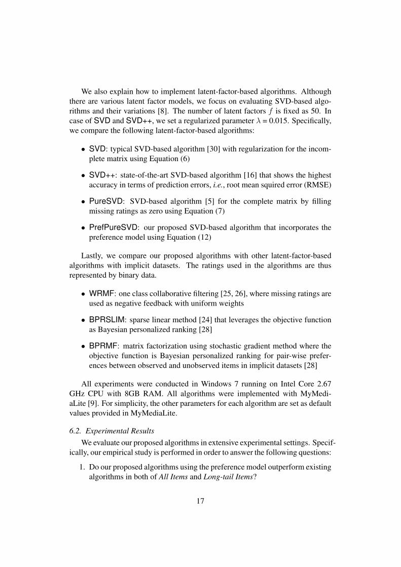
Figure 3: Comparison results of item-based algorithms in All Items over varying N (MovieLens1M)

5 10 15 20 250.05

0.1

0.15

0.2

0.25

0.3

0.35

0.4

N

P@

N

ItemPopularitySVDSVD++PureSVDPrefPureSVD

5 10 15 20 250

0.1

0.2

0.3

0.4

N

R@

N


5 10 15 20 25

0.1

0.2

0.3

0.4

0.5

NN

DC

G@

N



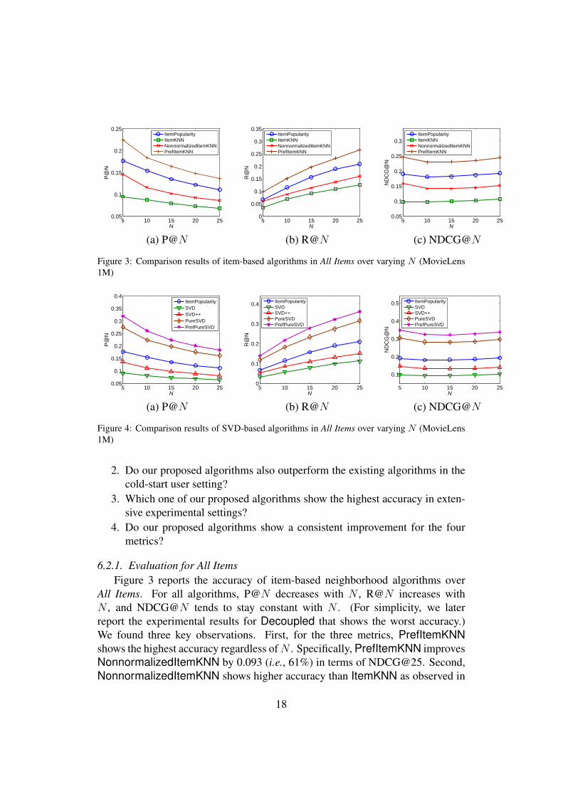
Figure 4: Comparison results of SVD-based algorithms in All Items over varying N (MovieLens1M)

2. Do our proposed algorithms also outperform the existing algorithms in thecold-start user setting?

3. Which one of our proposed algorithms show the highest accuracy in exten-sive experimental settings?

4. Do our proposed algorithms show a consistent improvement for the fourmetrics?

6.2.1. Evaluation for All ItemsFigure 3 reports the accuracy of item-based neighborhood algorithms over

All Items. For all algorithms, P@N decreases with N , R@N increases withN , and NDCG@N tends to stay constant with N . (For simplicity, we laterreport the experimental results for Decoupled that shows the worst accuracy.)We found three key observations. First, for the three metrics, PrefItemKNNshows the highest accuracy regardless ofN . Specifically, PrefItemKNN improvesNonnormalizedItemKNN by 0.093 (i.e., 61%) in terms of NDCG@25. Second,NonnormalizedItemKNN shows higher accuracy than ItemKNN as observed in

18

5 10 15 20 250.04

0.06

0.08

0.1

0.12

N

P@

N


5 10 15 20 250

0.05

0.1

0.15

0.2

N

R@

N


5 10 15 20 250.04

0.08

0.12

0.16

0.2

N

ND

CG

@N



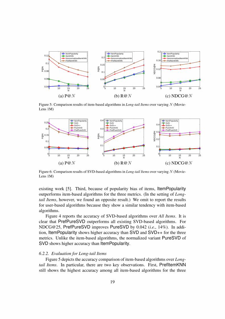
Figure 5: Comparison results of item-based algorithms in Long-tail Items over varying N (Movie-Lens 1M)

5 10 15 20 250

0.05

0.1

0.15

0.2

0.25

N

P@

N


5 10 15 20 250

0.1

0.2

0.3

0.4

N

R@

N


5 10 15 20 250

0.1

0.2

0.3

0.4

N

ND

CG

@N



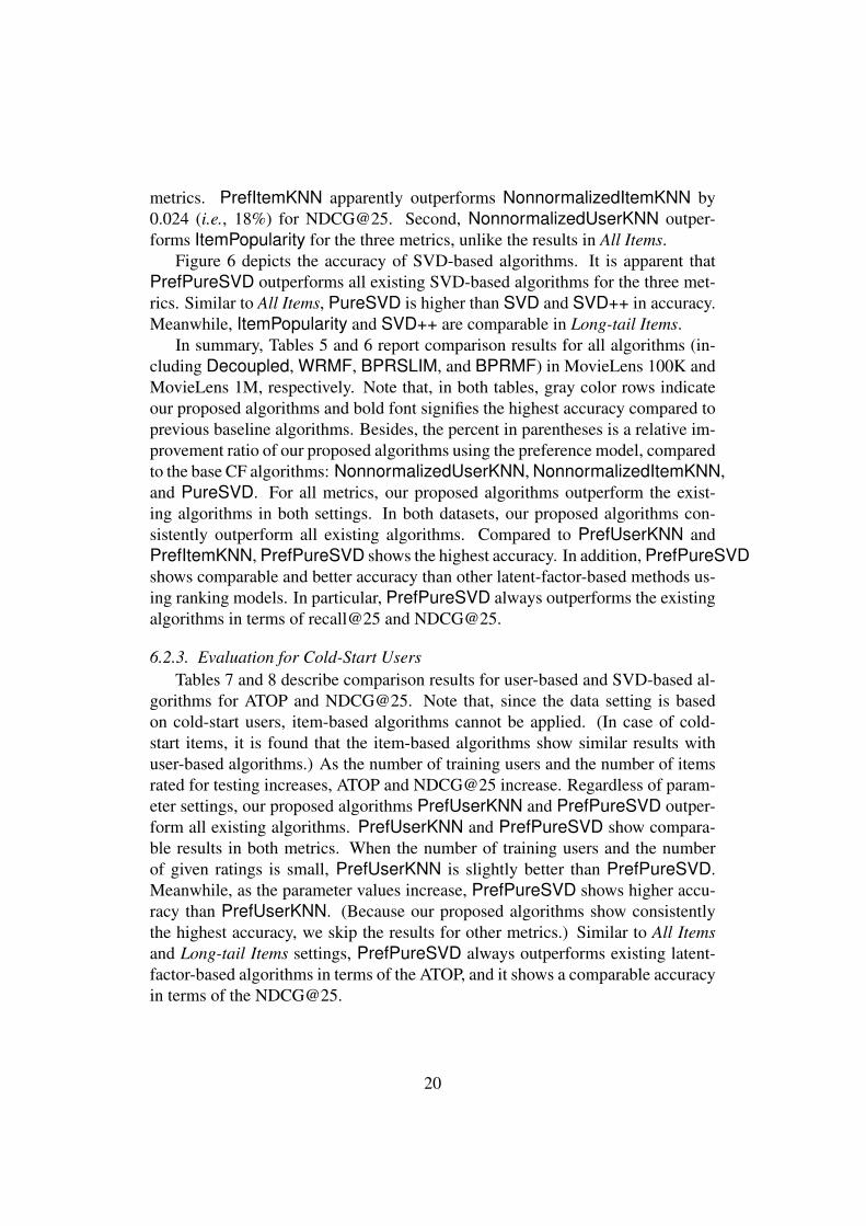
Figure 6: Comparison results of SVD-based algorithms in Long-tail Items over varying N (Movie-Lens 1M)

existing work [5]. Third, because of popularity bias of items, ItemPopularityoutperforms item-based algorithms for the three metrics. (In the setting of Long-tail Items, however, we found an opposite result.) We omit to report the resultsfor user-based algorithms because they show a similar tendency with item-basedalgorithms.

Figure 4 reports the accuracy of SVD-based algorithms over All Items. It isclear that PrefPureSVD outperforms all existing SVD-based algorithms. ForNDCG@25, PrefPureSVD improves PureSVD by 0.042 (i.e., 14%). In addi-tion, ItemPopularity shows higher accuracy than SVD and SVD++ for the threemetrics. Unlike the item-based algorithms, the normalized variant PureSVD ofSVD shows higher accuracy than ItemPopularity.

6.2.2. Evaluation for Long-tail ItemsFigure 5 depicts the accuracy comparison of item-based algorithms over Long-

tail Items. In particular, there are two key observations. First, PrefItemKNNstill shows the highest accuracy among all item-based algorithms for the three

19

metrics. PrefItemKNN apparently outperforms NonnormalizedItemKNN by0.024 (i.e., 18%) for NDCG@25. Second, NonnormalizedUserKNN outper-forms ItemPopularity for the three metrics, unlike the results in All Items.

Figure 6 depicts the accuracy of SVD-based algorithms. It is apparent thatPrefPureSVD outperforms all existing SVD-based algorithms for the three met-rics. Similar to All Items, PureSVD is higher than SVD and SVD++ in accuracy.Meanwhile, ItemPopularity and SVD++ are comparable in Long-tail Items.

In summary, Tables 5 and 6 report comparison results for all algorithms (in-cluding Decoupled, WRMF, BPRSLIM, and BPRMF) in MovieLens 100K andMovieLens 1M, respectively. Note that, in both tables, gray color rows indicateour proposed algorithms and bold font signifies the highest accuracy compared toprevious baseline algorithms. Besides, the percent in parentheses is a relative im-provement ratio of our proposed algorithms using the preference model, comparedto the base CF algorithms: NonnormalizedUserKNN, NonnormalizedItemKNN,and PureSVD. For all metrics, our proposed algorithms outperform the exist-ing algorithms in both settings. In both datasets, our proposed algorithms con-sistently outperform all existing algorithms. Compared to PrefUserKNN andPrefItemKNN, PrefPureSVD shows the highest accuracy. In addition, PrefPureSVDshows comparable and better accuracy than other latent-factor-based methods us-ing ranking models. In particular, PrefPureSVD always outperforms the existingalgorithms in terms of recall@25 and NDCG@25.

6.2.3. Evaluation for Cold-Start UsersTables 7 and 8 describe comparison results for user-based and SVD-based al-

gorithms for ATOP and NDCG@25. Note that, since the data setting is basedon cold-start users, item-based algorithms cannot be applied. (In case of cold-start items, it is found that the item-based algorithms show similar results withuser-based algorithms.) As the number of training users and the number of itemsrated for testing increases, ATOP and NDCG@25 increase. Regardless of param-eter settings, our proposed algorithms PrefUserKNN and PrefPureSVD outper-form all existing algorithms. PrefUserKNN and PrefPureSVD show compara-ble results in both metrics. When the number of training users and the numberof given ratings is small, PrefUserKNN is slightly better than PrefPureSVD.Meanwhile, as the parameter values increase, PrefPureSVD shows higher accu-racy than PrefUserKNN. (Because our proposed algorithms show consistentlythe highest accuracy, we skip the results for other metrics.) Similar to All Itemsand Long-tail Items settings, PrefPureSVD always outperforms existing latent-factor-based algorithms in terms of the ATOP, and it shows a comparable accuracyin terms of the NDCG@25.

20

Table 5: Evaluation of the accuracy of top-N recommendation (MovieLens 100K)

AlgorithmsAll Items

ATOP P@25 R@25 NDCG@25Decoupled 0.831 0.022 0.151 0.087

ItemPopularity 0.890 0.054 0.280 0.174UserKNN 0.791 0.006 0.030 0.011

NonnormalizedUserKNN 0.786 0.060 0.280 0.191PrefUserKNN 0.927 (18%) 0.081 (35%) 0.440 (57%) 0.297 (56%)

ItemKNN 0.812 0.042 0.184 0.106NonnormalizedItemKNN 0.749 0.046 0.205 0.137

PrefItemKNN 0.925 (24%) 0.077 (67%) 0.411 (101%) 0.272 (98%)SVD 0.752 0.037 0.166 0.102

SVD++ 0.803 0.046 0.215 0.124PureSVD 0.888 0.078 0.425 0.272

PrefPureSVD 0.930 (5%) 0.097 (24%) 0.500 (18%) 0.339 (25%)WRMF 0.942 0.092 0.490 0.320

BPRSLIM 0.915 0.066 0.383 0.238BPRMF 0.942 0.083 0.449 0.282

AlgorithmsLong-tail Items



NonnormalizedUserKNN 0.761 0.031 0.203 0.113PrefUserKNN 0.904 (19%) 0.044 (42%) 0.334 (65%) 0.188(66%)


PrefItemKNN 0.900 (18%) 0.041 (32%) 0.309 (54%) 0.175(46%)SVD 0.727 0.022 0.142 0.074

SVD++ 0.750 0.026 0.169 0.087PureSVD 0.879 0.053 0.394 0.226


BPRSLIM 0.889 0.039 0.312 0.166BPRMF 0.924 0.050 0.368 0.193

21

Table 6: Evaluation of the accuracy of top-N recommendation (MovieLens 1M)

AlgorithmsAll Items





PrefItemKNN 0.919 (22%) 0.136 (58%) 0.267 (67%) 0.245 (61%)SVD 0.818 0.064 0.113 0.103

SVD++ 0.842 0.080 0.151 0.140PureSVD 0.869 0.162 0.316 0.296


BPRSLIM 0.909 0.136 0.229 0.224BPRMF 0.937 0.185 0.288 0.296

AlgorithmsLong-tail Items





PrefItemKNN 0.900 (17%) 0.077 (19%) 0.189 (29%) 0.155(18%)SVD 0.790 0.039 0.093 0.070

SVD++ 0.796 0.043 0.100 0.076PureSVD 0.899 0.126 0.318 0.275


BPRSLIM 0.889 0.089 0.181 0.157BPRMF 0.923 0.117 0.219 0.197

22

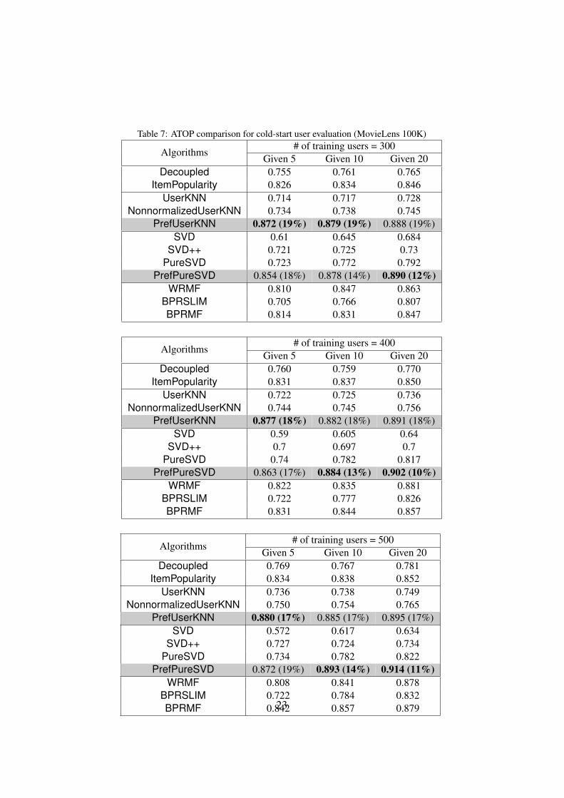
Table 7: ATOP comparison for cold-start user evaluation (MovieLens 100K)

Algorithms# of training users = 300

Given 5 Given 10 Given 20Decoupled 0.755 0.761 0.765

ItemPopularity 0.826 0.834 0.846UserKNN 0.714 0.717 0.728

NonnormalizedUserKNN 0.734 0.738 0.745PrefUserKNN 0.872 (19%) 0.879 (19%) 0.888 (19%)

SVD 0.61 0.645 0.684SVD++ 0.721 0.725 0.73

PureSVD 0.723 0.772 0.792PrefPureSVD 0.854 (18%) 0.878 (14%) 0.890 (12%)

WRMF 0.810 0.847 0.863BPRSLIM 0.705 0.766 0.807BPRMF 0.814 0.831 0.847





SVD 0.59 0.605 0.64SVD++ 0.7 0.697 0.7







SVD 0.572 0.617 0.634SVD++ 0.727 0.724 0.734



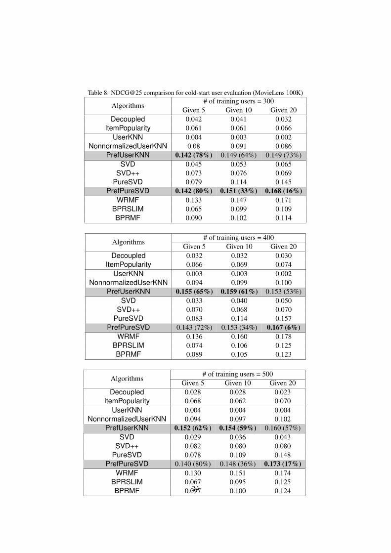
Table 8: NDCG@25 comparison for cold-start user evaluation (MovieLens 100K)





SVD 0.045 0.053 0.065SVD++ 0.073 0.076 0.069







SVD 0.033 0.040 0.050SVD++ 0.070 0.068 0.070







SVD 0.029 0.036 0.043SVD++ 0.082 0.080 0.080



7. Conclusion

In this paper, we have studied how to improve the accuracy of top-N rec-ommendation. To address this problem, two key challenges arise: (1) how todistinguish user experience between observed and missing ratings and (2) how toinfer latent user preference for observed ratings. We first designed a preferencemodel based on the qualitative order of items. We then proposed a family of CFalgorithms that combine the preference model with existing CF algorithms: user-based neighborhood, item-based neighborhood, and matrix-factorization-basedalgorithms. The empirical study showed that our proposed algorithms improvedthe existing algorithms by 3%–24%, 7%–67%, 8%–101%, and 6%–98% for ATOP,P@25, R@25, and NDCG@25, respectively.

In future work, we plan to consider two directions to further improve the ac-curacy of our proposed algorithms. First, we considered all missing ratings asnegative feedback. Inspired by one class collaborative filtering [25, 26], we planto distinguish the weight of missing ratings based on the confidence of negativefeedback. We hope that such a fine-grained distinction scheme for negative feed-back can contribute to the improvement of accuracy. Second, we plan to com-bine our proposed preference model with a pair-wise ranking model of items inBayesian personalized ranking [28]. We expect that such an idea can representrelative preferences more effectively.

References

[1] Gediminas Adomavicius and Alexander Tuzhilin. Toward the next genera-tion of recommender systems: A survey of the state-of-the-art and possibleextensions. IEEE Trans. Knowl. Data Eng., 17(6):734–749, 2005.

[2] Suhrid Balakrishnan and Sumit Chopra. Collaborative ranking. In WSDM,pages 143–152, 2012.

[3] Alejandro Bellogın, Pablo Castells, and Ivan Cantador. Precision-orientedevaluation of recommender systems: an algorithmic comparison. In RecSys,pages 333–336, 2011.

[4] Andras A. Benczur and Miklos Kurucz. Who rated what? a recommendersystem benchmark winner report. ERCIM News, 2008(73), 2008.

[5] Paolo Cremonesi, Yehuda Koren, and Roberto Turrin. Performance of rec-ommender algorithms on top-N recommendation tasks. In RecSys, pages39–46, 2010.

25

[6] Mukund Deshpande and George Karypis. Item-based top-N recommenda-tion algorithms. ACM Trans. Inf. Syst., 22(1):143–177, 2004.

[7] Peter Emerson. The original borda count and partial voting. Social Choiceand Welfare, 40(2):353–358, 2013.

[8] Simon Funk. Netflix update: Try this at home, 2006.

[9] Zeno Gantner, Steffen Rendle, Christoph Freudenthaler, and Lars Schmidt-Thieme. Mymedialite: a free recommender system library. In RecSys, pages305–308, 2011.

[10] Jonathan L. Herlocker, Joseph A. Konstan, Al Borchers, and John Riedl.An algorithmic framework for performing collaborative filtering. In SIGIR,pages 230–237, 1999.

[11] Thomas Hofmann. Latent semantic models for collaborative filtering. ACMTrans. Inf. Syst., 22(1):89–115, 2004.

[12] Yi-Chung Hu. Recommendation using neighborhood methods withpreference-relation-based similarity. Inf. Sci., 284:18–30, 2014.

[13] Yifan Hu, Yehuda Koren, and Chris Volinsky. Collaborative filtering forimplicit feedback datasets. In ICDM, pages 263–272, 2008.

[14] Rong Jin, Luo Si, ChengXiang Zhai, and James P. Callan. Collaborativefiltering with decoupled models for preferences and ratings. In CIKM, pages309–316, 2003.

[15] Yehuda Koren. Collaborative filtering with temporal dynamics. In KDD,pages 447–456, 2009.

[16] Yehuda Koren. Factor in the neighbors: Scalable and accurate collaborativefiltering. TKDD, 4(1), 2010.

[17] Yehuda Koren, Robert M. Bell, and Chris Volinsky. Matrix factorizationtechniques for recommender systems. IEEE Computer, 42(8):30–37, 2009.

[18] Juntao Liu, Chenhong Sui, Dewei Deng, Junwei Wang, Bin Feng, WenyuLiu, and Caihua Wu. Representing conditional preference by boosted re-gression trees for recommendation. Inf. Sci., 327:1–20, 2016.

[19] Juntao Liu, Caihua Wu, Yi Xiong, and Wenyu Liu. List-wise probabilisticmatrix factorization for recommendation. Inf. Sci., 278:434–447, 2014.

26

[20] Nathan Nan Liu and Qiang Yang. Eigenrank: a ranking-oriented approachto collaborative filtering. In SIGIR, pages 83–90, 2008.

[21] Hao Ma, Irwin King, and Michael R. Lyu. Effective missing data predictionfor collaborative filtering. In SIGIR, pages 39–46, 2007.

[22] Benjamin M. Marlin and Richard S. Zemel. Collaborative prediction andranking with non-random missing data. In RecSys, pages 5–12, 2009.

[23] Benjamin M. Marlin, Richard S. Zemel, Sam T. Roweis, and MalcolmSlaney. Collaborative filtering and the missing at random assumption. InUAI, pages 267–275, 2007.

[24] Xia Ning and George Karypis. SLIM: sparse linear methods for top-n rec-ommender systems. In ICDM, pages 497–506, 2011.

[25] Rong Pan and Martin Scholz. Mind the gaps: weighting the unknown inlarge-scale one-class collaborative filtering. In KDD, pages 667–676, 2009.

[26] Rong Pan, Yunhong Zhou, Bin Cao, Nathan Nan Liu, Rajan M. Lukose,Martin Scholz, and Qiang Yang. One-class collaborative filtering. In ICDM,pages 502–511, 2008.

[27] Bruno Pradel, Nicolas Usunier, and Patrick Gallinari. Ranking with non-random missing ratings: influence of popularity and positivity on evaluationmetrics. In RecSys, pages 147–154, 2012.

[28] Steffen Rendle, Christoph Freudenthaler, Zeno Gantner, and Lars Schmidt-Thieme. BPR: bayesian personalized ranking from implicit feedback. InUAI, pages 452–461, 2009.

[29] Francesco Ricci, Lior Rokach, Bracha Shapira, and Paul B. Kantor. Recom-mender Systems Handbook. Springer, 2011.

[30] Ruslan Salakhutdinov and Andriy Mnih. Probabilistic matrix factorization.In NIPS, pages 1257–1264, 2007.

[31] Badrul M. Sarwar, George Karypis, Joseph A. Konstan, and John Riedl.Item-based collaborative filtering recommendation algorithms. In WWW,pages 285–295, 2001.

[32] Yue Shi, Martha Larson, and Alan Hanjalic. List-wise learning to rank withmatrix factorization for collaborative filtering. In RecSys, pages 269–272,2010.

27

[33] Yue Shi, Martha Larson, and Alan Hanjalic. Unifying rating-oriented andranking-oriented collaborative filtering for improved recommendation. Inf.Sci., 229:29–39, 2013.

[34] Harald Steck. Training and testing of recommender systems on data missingnot at random. In KDD, pages 713–722, 2010.

[35] Harald Steck. Item popularity and recommendation accuracy. In RecSys,pages 125–132, 2011.

[36] Harald Steck. Evaluation of recommendations: rating-prediction and rank-ing. In RecSys, pages 213–220, 2013.

[37] Xiaoyuan Su and Taghi M. Khoshgoftaar. A survey of collaborative filteringtechniques. Adv. Artificial Intellegence, 2009.

[38] Alvaro Tejeda-Lorente, Carlos Porcel, Eduardo Peis, Rosa Sanz, and En-rique Herrera-Viedma. A quality based recommender system to disseminateinformation in a university digital library. Inf. Sci., 261:52–69, 2014.

[39] Markus Weimer, Alexandros Karatzoglou, Quoc V. Le, and Alexander J.Smola. COFI RANK - maximum margin matrix factorization for collabora-tive ranking. In NIPS, pages 1593–1600, 2007.

28

Improving the Accuracy of Top-N Recommendation …pike.psu.edu/publications/is16-PrefCF.pdfImproving...

Documents

Transcript of Improving the Accuracy of Top-N Recommendation …pike.psu.edu/publications/is16-PrefCF.pdfImproving...