Improving Robustness Of Estimates From Non-Probability Online Samples

Dina Neiger, Andrew C. Ward and Darren W. Pennay

Workshop on Robust Inference for Sample Surveys,

University of Wollongong, 7 July 2017

www.srcentre.com.au

Motivation

• Weighting adjustments for non-probability samples:

• Usual approach: standard demographic post-

stratification (with or without RIM)

• Relatively little benefit for samples with demographic quotas

• Can increase bias

• Blending

• Very effective but expensive and not always practical

• Model-based design weights

• Worth the effort?

• Calibration

• What variables work best?

• Independent benchmarks not always available

• Difference between panels

• Value proposition?

3

www.srcentre.com.au

The Online Panels Benchmarking Study4

3 x surveys

➢ probability

samples

➢ Australian pop

aged 18+

5 x surveys

➢ Members non-

probability

online panels

➢ Aged 18+

➢ Oct-Dec 15

Questionnaire

included range of

demographic

questions and

questions about

health, wellbeing

and use of

technology

Standardised

questions were used

to mitigate mode

effects

Items were chosen because there were high

quality (e.g. ABS) population benchmarks

available for these measures

Data and documentation available from the

Australian Data Archive

www.ada.edu.au/ada/01329

www.srcentre.com.au

www.srcentre.com.au

Life in Australia, Design Features

Recruitment Oct-Nov 2016

• Dual-frame RDD (60% mobile

frame/40% landline frame)

• National probability

proportional to size sample

design

• Trialling different recruitment

methods (combinations of

incentives, materials, one and

two-stage recruitment)

Response maximisation

• Non-contingent incentive

• Extended routine / Reminders

Panel member

Advance notification postcard

3-week enumeration/multiple

reminders (email and text)

Panel dimensions

• N=3,000 approx.

• Aged 18 years and over

• Online and offline population

• English-speaking

Panel maintenance

• Sample top up via a single –

frame mobile phone survey

6

www.srcentre.com.au

Weighting (standard approach)

Design weight (Probability surveys only):➢ Adjusting for overlapping chance of selection (single-frame approach), number of

landlines, number of in-scope persons in household

➢ LinA includes propensity weight based on response probabilities

➢ Design weight of ‘1’ for the non-probability panels

Post stratification (Raking/RIM):➢ Gender

➢ Education by age (18-24 years, 25-34 years with/out university degree, 35-44 years

with/out university degree, 45-54 years with/out university degree, 55-64 years

with/out university degree, 65-74 years with/out university degree, 75 + years

with/out university degree

➢ Telephone status (Landline-only, Dual-users, Mobile-only)

➢ Volunteer (Yes/No)

➢ Future work to improve LinA estimates: include additional educational levels, State,

investigate optimal post-stratification variables post Census 2016 data release

8

www.srcentre.com.au

Method

➢ Yeager, D. S., Krosnick, J.

A., Chang, L., Javitz, H. S.,

Levendusky, M. S.,

Simpser, A., (2011). Comparing the Accuracy of RDD

Telephone Surveys and Internet

Surveys Conducted with Probability and

Non-Probability Samples. Public

Opinion Quarterly

➢ Average absolute error to

compare to benchmarks

o Average of absolute differences

(percentage points) across all

measures between the benchmark

and the survey estimate

9

Comparison

Compare probability and non-

probability surveysMethodResults

➢ Probability and non-

probability surveys perform

similarly well with respect to

demographics

➢ for substantive characteristics

the probability surveys are

more accurate

www.srcentre.com.au

Results – substantive characteristics10

Substantive variablesBenchmark

value (%)

Distance from benchmarks (percentage point difference from

benchmark)

LinA

Dual

Frame

Prob.

Non-probability Panels

1 2 3 4 5

Life satisfaction

(8 out of 10)32.6 -1.4 2.2 -11.1 -13.6 -5.9 -10.3 -8.0

Psychological distress -

Kessler 6 (Low)82.2 -21.3 -9.8 -26.5 -25.5 -22.7 -25.1 -23.4

General Health Status -

SF1 (Very good) 36.2 -3.8 -5.0 -4.2 -4.2 -4.0 -5.3 0.1

Private Health Insurance 57.1 2.6 3.9 -8.0 -9.8 -3.9 0.1 -2.0

Daily smoker 13.5 -1.0 2.1 9.0 6.0 3.5 2.2 3.5

Consumed alcohol in the

last 12 months81.9 2.7 3.0 -1.1 -6.4 -3.6 -4.9 -1.7

Enrolled to vote 78.5 9.0 8.3 8.4 7.6 10.7 8.8 13.1

www.srcentre.com.au

Method

➢ DiSogra, C., Cobb C., Chan

E., Dennis J. M. (2011) Calibrating Non-Probability Internet

Samples with Probability Samples

Using Early Adopter Characteristics.

Section on Survey Research Methods –

JSM 2011

➢ Blending probability and non-

probability surveys

➢ Use measures of early

adopter behaviours in

calibration

➢ Experiment with different

weighting variables

11

Initial calibration

Compare probability and non-

probability surveysMethodResults

➢ Reduction in bias is mostly

due to blending but not always

practical

➢ Use the best probability

sample to combine with non

probability regardless of mode

and response rate

www.srcentre.com.au

Extend calibration methodology to12

Include other significant

differentiators in the

calibration

➢ Fahimi, M., F. M.

Barlas, R. K. Thomas

and N. Buttermore

(2015) Scientific Surveys Based on

Incomplete Sampling

Frames and High Rates of

Nonresponse. Survey

Practice. 8 (5)

➢ Find demographic,

behavioural and

attitudinal measures

that differentiate

between probability

and non-probability

panels

Model probability of

appearing in non-

probability sample

➢ Valliant, R., Dever, J.

A. (2011)Estimating propensity

adjustments for volunteer

web surveys, Sociological

Methods & Research, 40(1),

pp. 105-137)

➢ Use propensity-

response model to

calculate probability-

based design weight

for non-probability

sample

➢ Terhnian, G., Bremer,

J., Haney C., (2014) A model based approach for

achieving a representative

sample

➢ Average of the

“average absolute

errors” and “mean

square errors” across

multiple panels when

comparing weighting

methods

Compare effectiveness of

methods using multiple

samples

www.srcentre.com.au

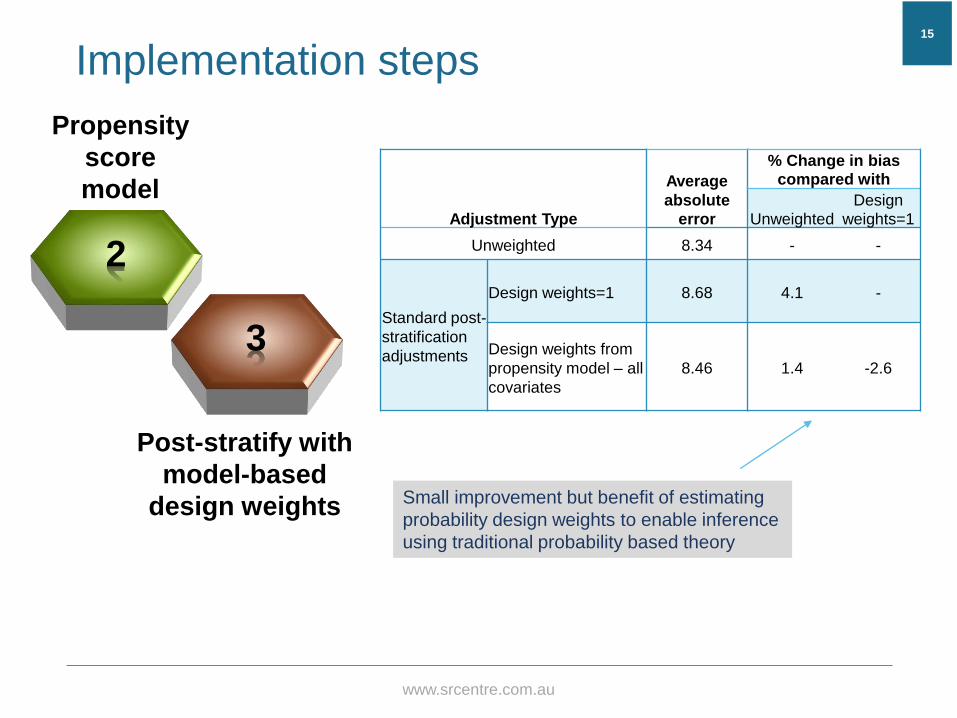
1

Post-stratify

reference

sample

Implementation steps

Adjust for coverage and non-response bias

• Raking (“rim weighting”)

• Include Volunteerism

• Keep number of variables to a minimum

13

www.srcentre.com.au

2

Propensity

score

model

1

Post-stratify

reference

sample

Implementation steps

Calculate probability based design weights

for non-probability samples:

▪ Non-probability cases=1, reference

cases=0

▪ Design weight - inverse of estimated

probability of inclusion in non-probability

sample given weighted reference

sample

▪ Use as many covariates as available

(exclude measures being evaluated)

Issues encountered:

▪ Extremely small probability for some

cases => to extremely large weights

(even when using propensity class

mean)

▪ Solution: trim design weights

14

www.srcentre.com.au

2

Propensity

score

model

3

Post-stratify with

model-based

design weights

Implementation steps

Adjustment Type

Average

absolute

error

% Change in bias compared with

Unweighted

Design

weights=1

Unweighted 8.34 - -

Standard post-

stratification

adjustments

Design weights=1 8.68 4.1 -

Design weights from

propensity model – all

covariates

8.46 1.4 -2.6

15

Small improvement but benefit of estimating

probability design weights to enable inference

using traditional probability based theory

www.srcentre.com.au

3

Post-stratify

with mode-

based

design

weights

Implementation steps

Compare estimates post-stratified reference sample with the post-stratified non-probability sample and test for significant differences.

Significantly different for all 5 panels (compared to the reference sample)

✓ Early adopter variables

✓ Internet usage variables

✓ Income

✓ Employment

✓ Remoteness

(was not a factor in RDD, LinA – larger sample)

✓ Home ownership

4

Find significant

differentiators

17

www.srcentre.com.au

6

Evaluate

5

Add key

differentiators

Implementation steps

Compare average absolute error and root mean square error across five non-probability panels for 7 outcome measures:

➢ General health status (ABS National Health Survey)

➢ Psychological distress (ABS National Health Survey)

➢ Life satisfaction (ABS General Social Survey)

➢ Private health insurance coverage (ABS National Health Survey)

➢ Daily smoking status (AIHW National Drug Strategy Household Survey)

➢ Alcohol consumption in the last 12 months (AIHW National Drug Strategy Household Survey)

➢ Enrolled to vote (Australian Electoral Commission)

18

www.srcentre.com.au

Early Adopter Characteristics

DiSogra et al. (2011) “Early adopters (EA) – consumers

who embrace new technology and products sooner than

most others”

EA1: I usually try new products before other people do

EA2: I often try new brands because I like variety and

get bored with the same old thing

EA3: When I shop I look for what is new

EA4: I like to be the first among my friends and family to

try something new

EA5: I like to tell others about new brands or technology

19

www.srcentre.com.au

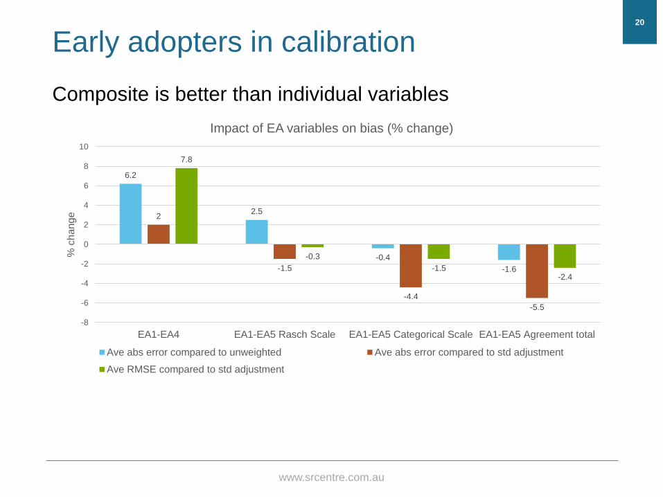
Early adopters in calibration

Composite is better than individual variables

20

6.2

2.5

-0.4

-1.6

2

-1.5

-4.4

-5.5

7.8

-0.3

-1.5-2.4

-8

-6

-4

-2

0

2

4

6

8

10

EA1-EA4 EA1-EA5 Rasch Scale EA1-EA5 Categorical Scale EA1-EA5 Agreement total

% c

han

ge

Impact of EA variables on bias (% change)

Ave abs error compared to unweighted Ave abs error compared to std adjustment

Ave RMSE compared to std adjustment

www.srcentre.com.au

Internet usage measures

Look for information:How often look for information over the internet

Access a home:Type of internet connection

Post to blogs etc:How often - Post to blog/forums/interest groups

Financial transactions:How often - Conduct financial transactions such as banking over the Internet

Social media:How often - Comment or post images to social media sites (Facebook, Twitter, etc.)

Frequency of use:How often - Use the Internet at work, home or elsewhere

21

www.srcentre.com.au

Internet usage measures

Not useful when calibrating online to online

22

2.6

5

4.5

5.5

-1.5

0.9

0.3

1.3

0.1

2

6.4

1.9

-2

-1

0

1

2

3

4

5

6

7

Look for information Access at home, Look forinformation

Look for information, Post toblogs etc, Financial

transactions, Social Media

Access at home, Frequency of use

% c

han

ge

Impact of Internet Usage measures on bias (% change)

Ave abs error compared to unweighted Ave abs error compared to std adjustment

Ave RMSE compared to std adjustment

www.srcentre.com.au

Other differentiators

Income: Annual income pre-tax:

Employment:In the last week, any work done in a job, business or farm, without pay in a family

business, including away from because of holidays, sickness or any other reason

Home ownership: Remoteness:

23

$2,000 or more per week ($104,000 or more per year)

$1,500 - $1,999 per week ($78,000 - $103,999 per year)

$1,250 - $1,499 per week ($65,000 - $77,999 per year)

$1,000 - $1,249 per week ($52,000 - $64,999 per year)

$800 - $999 per week ($41,600 - $51,999 per year)

$600 - $799 per week ($31,200 - $41,599 per year)

$400 - $599 per week ($20,800 - $31,199 per year)

$300 - $399 per week ($15,600 - $20,799 per year)

$200 - $299 per week ($10,400 - $15,599 per year)

$1 - $199 per week ($1 - $10,399 per year)

Nil income/Negative income

Owned outright

Owned with a mortgage

Being purchased under a rent/buy scheme

Being rented

Being occupied rent free

Being occupied under a life tenure scheme

Other

Major Cities

Inner Regional

Other (Outer Regional, Remote, Very

Remote, Not answered)

www.srcentre.com.au

Other DifferentiatorsIncome – single most influential variable to reduce bias and RMSE

Benefit from including both: income and employment

24

-7.3

-10.3

-7.3

-5.9

-11.0

-13.9

-10.9

-9.6

-8.5

-10.6

-5.8

-4.6

-16.0

-14.0

-12.0

-10.0

-8.0

-6.0

-4.0

-2.0

0.0

Income Income, Employment Income, Employment, HomeOwnership

Income, Employment, HomeOwnership, Remoteness

% c

han

ge

Impact of Income, Employment and Home Ownership variables on bias (% change)

Ave abs error compared to unweighted Ave abs error compared to std adjustment Ave RMSE compared to std adjustment

www.srcentre.com.au

Combine EA, Income and Employment

Std adjustments: Telephone status, Age by Education, Gender, Volunteer

Design weights model: Primary demographics, Secondary demographics, Telephone

status, Volunteer, EA (individual), Internet use (all)

Key differentiations: Income, Employment, EA total agreement score

25

Adjustment Type

Average

absolute

error

% Change in

bias cf

unweighted

% Change in bias cf

weighted with std

adjustments

Average

RMSE

% Change in

RMSE cf

weighted with std

adjustments

Unweighted 8.34

Weighted with std

adjustments8.68 4.10 9.10

Weighted with design

weights and std

adjustments

8.46 1.40 -2.60 8.96 -1.50

Weighted with design

weights and key

differentiators

7.47 -10.40 -13.90 8.31 -8.60

www.srcentre.com.au

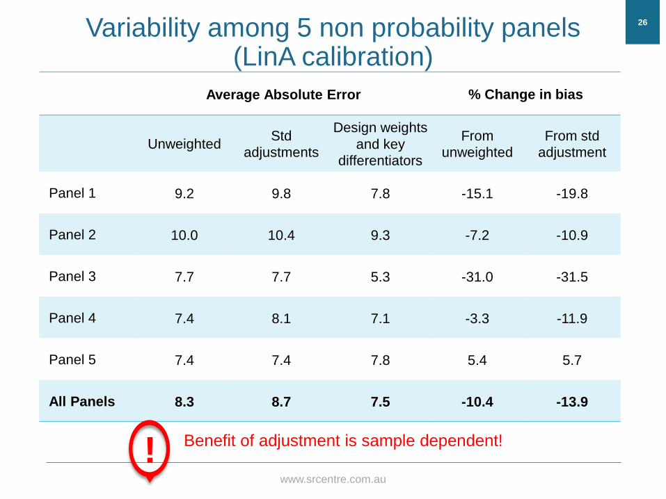
Variability among 5 non probability panels(LinA calibration)

Average Absolute Error % Change in bias

UnweightedStd

adjustments

Design weights

and key

differentiators

From

unweighted

From std

adjustment

Panel 1 9.2 9.8 7.8 -15.1 -19.8

Panel 2 10.0 10.4 9.3 -7.2 -10.9

Panel 3 7.7 7.7 5.3 -31.0 -31.5

Panel 4 7.4 8.1 7.1 -3.3 -11.9

Panel 5 7.4 7.4 7.8 5.4 5.7

All Panels 8.3 8.7 7.5 -10.4 -13.9

26

Benefit of adjustment is sample dependent!!

www.srcentre.com.au

Variability among 5 non probability panels(RDD calibration)

Average Absolute Error % Change in bias

UnweightedStd

adjustments

Design weights

and key

differentiators

From

unweighted

From std

adjustment

Panel 1 9.2 9.8 6.7 -27.3 -31.4

Panel 2 10.0 10.4 8.3 -17.2 -20.5

Panel 3 7.7 7.7 5.5 -29.0 -29.6

Panel 4 7.4 8.1 7.5 2.4 -6.7

Panel 5 7.4 7.4 7.1 -4.0 -3.8

All Panels 8.3 8.7 7.0 -15.8 -19.1

27

Benefit of adjustment is sample dependent!!

www.srcentre.com.au

Comparison with independent benchmarks vs reference sample benchmarks

28

Mostly change in bias is consistent but there can be large differences for some samples

-15.1

-7.2

-31.0

-3.3

5.4

-26.9

5.7

-31.7

28.7

1.0

-40.0

-30.0

-20.0

-10.0

0.0

10.0

20.0

30.0

40.0

Panel 1 Panel 2 Panel 3 Panel 4 Panel 5

% Change in bias from unweighted

Independent Benchmarks Reference Sample

-19.8

-10.9

-31.5

-11.9

5.7

-30.6

0.6

-31.5

-12.4-8.3

-50.0

-40.0

-30.0

-20.0

-10.0

0.0

10.0

20.0

Panel 1 Panel 2 Panel 3 Panel 4 Panel 5

% Change in bias from std adjustment

Independent Benchmarks Reference Sample

www.srcentre.com.au

Combination of

➢ A robust reference sample

with enough variables in

common

➢ Application of propensity

scores to calculate design

based probabilities

➢ Extending calibration

variables to include key

differentiators (beyond EA

and internet use)

➢ Good population benchmarks

➢ A bit of time and statistical

“know how”

29

In conclusion…

Will improve quality of inference

from a non-probability sample

but not a magic bullet

➢ Adjustments need to be

developed for each sample

➢ Plan ahead to include

sufficient calibration variables

in reference and non-

probability sample

➢ Aim to include at least some

independent benchmarks

www.srcentre.com.au

Where to next…

30

www.srcentre.com.au

Now that probability online

panel is available

Repeat analysis with Life in

Australia as the reference

sample

➢ ~2,500 respondents in the

first two waves

➢ No mode issues

31

Scope to

➢ Systematise and

standardise approach

➢ Trial other key

differentiators identified in

the literature (e.g. media

exposure, alternative

income measures)

➢ Optimisation (Terhanian et

al) for selection of best

combination of calibration

variables

Ideas and suggestions from the workshop

Thank you

Contact: Andrew Ward (andrew.ward@srcentre.com.au)