This document and trademark(s) contained herein are protected by law as indicated in a notice appearing later in this work. This electronic representation of RAND intellectual property is provided for non-commercial use only. Unauthorized posting of RAND PDFs to a non-RAND Web site is prohibited. RAND PDFs are protected under copyright law. Permission is required from RAND to reproduce, or reuse in another form, any of our research documents for commercial use. For information on reprint and linking permissions, please see RAND Permissions.

Limited Electronic Distribution Rights

This PDF document was made available from www.rand.org as a public

service of the RAND Corporation.

6Jump down to document

THE ARTS

CHILD POLICY

CIVIL JUSTICE

EDUCATION

ENERGY AND ENVIRONMENT

HEALTH AND HEALTH CARE

INTERNATIONAL AFFAIRS

NATIONAL SECURITY

POPULATION AND AGING

PUBLIC SAFETY

SCIENCE AND TECHNOLOGY

SUBSTANCE ABUSE

TERRORISM AND HOMELAND SECURITY

TRANSPORTATION ANDINFRASTRUCTURE

WORKFORCE AND WORKPLACE

The RAND Corporation is a nonprofit research organization providing objective analysis and effective solutions that address the challenges facing the public and private sectors around the world.

Visit RAND at www.rand.org

Explore RAND Arroyo Center

View document details

For More Information

Purchase this document

Browse Books & Publications

Make a charitable contribution

Support RAND

This product is part of the RAND Corporation technical report series. Reports may

include research findings on a specific topic that is limited in scope; present discus-

sions of the methodology employed in research; provide literature reviews, survey

instruments, modeling exercises, guidelines for practitioners and research profes-

sionals, and supporting documentation; or deliver preliminary findings. All RAND

reports undergo rigorous peer review to ensure that they meet high standards for re-

search quality and objectivity.

Improving Recapitalization Planning

Toward a Fleet Management Model for the High-Mobility Multipurpose Wheeled Vehicle

Ellen M. Pint • Lisa Pelled Colabella • Justin L. Adams • Sally Sleeper

Prepared for the United States Army Approved for public release; distribution unlimited

The RAND Corporation is a nonprofit research organization providing objective analysis and effective solutions that address the challenges facing the public and private sectors around the world. RAND’s publications do not necessarily reflect the opinions of its research clients and sponsors.

R® is a registered trademark.

© Copyright 2008 RAND Corporation

All rights reserved. No part of this book may be reproduced in any form by any electronic or mechanical means (including photocopying, recording, or information storage and retrieval) without permission in writing from RAND.

Published 2008 by the RAND Corporation1776 Main Street, P.O. Box 2138, Santa Monica, CA 90407-2138

1200 South Hayes Street, Arlington, VA 22202-50504570 Fifth Avenue, Suite 600, Pittsburgh, PA 15213-2665

RAND URL: http://www.rand.orgTo order RAND documents or to obtain additional information, contact

Distribution Services: Telephone: (310) 451-7002; Fax: (310) 451-6915; Email: order@rand.org

The research described in this report was sponsored by the United States Army under Contract No. DASW01-01-C-0003.

Library of Congress Cataloging-in-Publication Data is available for this publication.

ISBN 978-0-8330-4174-6

iii

Preface

The Army is undergoing a major transformation to ensure that its future capabilities can meet the needs of the nation. A prominent element of its transformation strategy is the recapitaliza-tion (RECAP) program, which entails rebuilding and selectively upgrading 17 systems. The RECAP program has continuously evolved, with ongoing decisionmaking about the types of system modifications that will occur and the scale of programs. This document describes a study conducted by the RAND Corporation to help inform RECAP decisions.

The researchers used a two-part methodology to develop a decision-support tool to facili-tate RECAP planning and demonstrated its application using high-mobility multipurpose wheeled vehicle (HMMWV) data. They first assessed the effects of vehicle age and other key predictor variables on HMMWV repair costs and downtime; they then embedded the results in a vehicle replacement model to estimate optimal replacement or RECAP age. The findings of this study should be of interest to Army logisticians, acquisition personnel, and resource planners.

This research, part of a project entitled “Improving Recapitalization Planning,” was sponsored by the Deputy Chief of Staff, G-4, Department of the Army, and was conducted within RAND Arroyo Center’s Military Logistics Program. RAND Arroyo Center, part of the RAND Corporation, is a federally funded research and development center sponsored by the United States Army.

The Project Unique Identification Code (PUIC) for the project that produced this docu-ment is DAPRRY021.

iv Improving Recapitalization Planning: Toward a Fleet Management Model for the HMMWV

For more information on RAND Arroyo Center, contact the Director of Operations (tele-phone 310-393-0411, extension 6419; fax 310-451-6952; email Marcy_Agmon@rand.org), or visit Arroyo’s web site at http://www.rand.org/ard/.

v

Contents

Preface . . . . . . . . . . . . . . . . . . . . . . . . . . . . . . . . . . . . . . . . . . . . . . . . . . . . . . . . . . . . . . . . . . . . . . . . . . . . . . . . . . . . . . . . . . . . . . . . . . . . . . . . . . . iiiFigures . . . . . . . . . . . . . . . . . . . . . . . . . . . . . . . . . . . . . . . . . . . . . . . . . . . . . . . . . . . . . . . . . . . . . . . . . . . . . . . . . . . . . . . . . . . . . . . . . . . . . . . . . . . viiTables . . . . . . . . . . . . . . . . . . . . . . . . . . . . . . . . . . . . . . . . . . . . . . . . . . . . . . . . . . . . . . . . . . . . . . . . . . . . . . . . . . . . . . . . . . . . . . . . . . . . . . . . . . . . ixSummary . . . . . . . . . . . . . . . . . . . . . . . . . . . . . . . . . . . . . . . . . . . . . . . . . . . . . . . . . . . . . . . . . . . . . . . . . . . . . . . . . . . . . . . . . . . . . . . . . . . . . . . . xiAcknowledgments . . . . . . . . . . . . . . . . . . . . . . . . . . . . . . . . . . . . . . . . . . . . . . . . . . . . . . . . . . . . . . . . . . . . . . . . . . . . . . . . . . . . . . . . . . . . . xvAbbreviations . . . . . . . . . . . . . . . . . . . . . . . . . . . . . . . . . . . . . . . . . . . . . . . . . . . . . . . . . . . . . . . . . . . . . . . . . . . . . . . . . . . . . . . . . . . . . . . . . xvii

CHAPTER ONE

Introduction . . . . . . . . . . . . . . . . . . . . . . . . . . . . . . . . . . . . . . . . . . . . . . . . . . . . . . . . . . . . . . . . . . . . . . . . . . . . . . . . . . . . . . . . . . . . . . . . . . . . . 1

CHAPTER TWO

Predicting the Effects of Aging on HMMWV Costs and Availability . . . . . . . . . . . . . . . . . . . . . . . . . . . . . . . . 5Sample Characteristics. . . . . . . . . . . . . . . . . . . . . . . . . . . . . . . . . . . . . . . . . . . . . . . . . . . . . . . . . . . . . . . . . . . . . . . . . . . . . . . . . . . . . . . . . . . 5Measures and Data Sources . . . . . . . . . . . . . . . . . . . . . . . . . . . . . . . . . . . . . . . . . . . . . . . . . . . . . . . . . . . . . . . . . . . . . . . . . . . . . . . . . . . . . 6

Age . . . . . . . . . . . . . . . . . . . . . . . . . . . . . . . . . . . . . . . . . . . . . . . . . . . . . . . . . . . . . . . . . . . . . . . . . . . . . . . . . . . . . . . . . . . . . . . . . . . . . . . . . . . . . . 8Annual Usage . . . . . . . . . . . . . . . . . . . . . . . . . . . . . . . . . . . . . . . . . . . . . . . . . . . . . . . . . . . . . . . . . . . . . . . . . . . . . . . . . . . . . . . . . . . . . . . . . . . 8Vehicle Type . . . . . . . . . . . . . . . . . . . . . . . . . . . . . . . . . . . . . . . . . . . . . . . . . . . . . . . . . . . . . . . . . . . . . . . . . . . . . . . . . . . . . . . . . . . . . . . . . . . . 9Location . . . . . . . . . . . . . . . . . . . . . . . . . . . . . . . . . . . . . . . . . . . . . . . . . . . . . . . . . . . . . . . . . . . . . . . . . . . . . . . . . . . . . . . . . . . . . . . . . . . . . . . . . 9Odometer Reading . . . . . . . . . . . . . . . . . . . . . . . . . . . . . . . . . . . . . . . . . . . . . . . . . . . . . . . . . . . . . . . . . . . . . . . . . . . . . . . . . . . . . . . . . . . . 9Downtime . . . . . . . . . . . . . . . . . . . . . . . . . . . . . . . . . . . . . . . . . . . . . . . . . . . . . . . . . . . . . . . . . . . . . . . . . . . . . . . . . . . . . . . . . . . . . . . . . . . . . . 9EDA-Based Repair Costs . . . . . . . . . . . . . . . . . . . . . . . . . . . . . . . . . . . . . . . . . . . . . . . . . . . . . . . . . . . . . . . . . . . . . . . . . . . . . . . . . . . . . 9

Regression Analyses . . . . . . . . . . . . . . . . . . . . . . . . . . . . . . . . . . . . . . . . . . . . . . . . . . . . . . . . . . . . . . . . . . . . . . . . . . . . . . . . . . . . . . . . . . . . . 12Two-Part “Hurdle” Cost and Downtime Regressions . . . . . . . . . . . . . . . . . . . . . . . . . . . . . . . . . . . . . . . . . . . . . . . . . . . . 12

CHAPTER THREE

Estimation Results . . . . . . . . . . . . . . . . . . . . . . . . . . . . . . . . . . . . . . . . . . . . . . . . . . . . . . . . . . . . . . . . . . . . . . . . . . . . . . . . . . . . . . . . . . . . . 17Cost Versus Age . . . . . . . . . . . . . . . . . . . . . . . . . . . . . . . . . . . . . . . . . . . . . . . . . . . . . . . . . . . . . . . . . . . . . . . . . . . . . . . . . . . . . . . . . . . . . . . . . 17Comparisons of Predicted and Observed Costs Versus Age . . . . . . . . . . . . . . . . . . . . . . . . . . . . . . . . . . . . . . . . . . . . . . 20Downtime Versus Age . . . . . . . . . . . . . . . . . . . . . . . . . . . . . . . . . . . . . . . . . . . . . . . . . . . . . . . . . . . . . . . . . . . . . . . . . . . . . . . . . . . . . . . . . 22Odometer Reading Versus Age . . . . . . . . . . . . . . . . . . . . . . . . . . . . . . . . . . . . . . . . . . . . . . . . . . . . . . . . . . . . . . . . . . . . . . . . . . . . . . . 24

vi Improving Recapitalization Planning: Toward a Fleet Management Model for the HMMWV

CHAPTER FOUR

Application of the Vehicle Replacement Model . . . . . . . . . . . . . . . . . . . . . . . . . . . . . . . . . . . . . . . . . . . . . . . . . . . . . . . . . 27Overview of the VaRooM Vehicle Replacement Model . . . . . . . . . . . . . . . . . . . . . . . . . . . . . . . . . . . . . . . . . . . . . . . . . . . 27VaRooM Model Inputs Derived from Regression Estimates . . . . . . . . . . . . . . . . . . . . . . . . . . . . . . . . . . . . . . . . . . . . . 30

Number of Vehicles by Age . . . . . . . . . . . . . . . . . . . . . . . . . . . . . . . . . . . . . . . . . . . . . . . . . . . . . . . . . . . . . . . . . . . . . . . . . . . . . . . . . 30Estimated Odometer Reading by Age . . . . . . . . . . . . . . . . . . . . . . . . . . . . . . . . . . . . . . . . . . . . . . . . . . . . . . . . . . . . . . . . . . . . . 30Annual Mileage by Age . . . . . . . . . . . . . . . . . . . . . . . . . . . . . . . . . . . . . . . . . . . . . . . . . . . . . . . . . . . . . . . . . . . . . . . . . . . . . . . . . . . . . . 31Estimated Annual Down Days by Age . . . . . . . . . . . . . . . . . . . . . . . . . . . . . . . . . . . . . . . . . . . . . . . . . . . . . . . . . . . . . . . . . . . . . 31Estimated Annual Parts and Labor Cost by Age . . . . . . . . . . . . . . . . . . . . . . . . . . . . . . . . . . . . . . . . . . . . . . . . . . . . . . . . . . 31

Economic Parameters . . . . . . . . . . . . . . . . . . . . . . . . . . . . . . . . . . . . . . . . . . . . . . . . . . . . . . . . . . . . . . . . . . . . . . . . . . . . . . . . . . . . . . . . . . . 32Replacement Cost . . . . . . . . . . . . . . . . . . . . . . . . . . . . . . . . . . . . . . . . . . . . . . . . . . . . . . . . . . . . . . . . . . . . . . . . . . . . . . . . . . . . . . . . . . . . . 33Cost of Downtime . . . . . . . . . . . . . . . . . . . . . . . . . . . . . . . . . . . . . . . . . . . . . . . . . . . . . . . . . . . . . . . . . . . . . . . . . . . . . . . . . . . . . . . . . . . . 33Annual Discount Rate . . . . . . . . . . . . . . . . . . . . . . . . . . . . . . . . . . . . . . . . . . . . . . . . . . . . . . . . . . . . . . . . . . . . . . . . . . . . . . . . . . . . . . 34Depreciation Rates . . . . . . . . . . . . . . . . . . . . . . . . . . . . . . . . . . . . . . . . . . . . . . . . . . . . . . . . . . . . . . . . . . . . . . . . . . . . . . . . . . . . . . . . . . . . 35Salvage Factor . . . . . . . . . . . . . . . . . . . . . . . . . . . . . . . . . . . . . . . . . . . . . . . . . . . . . . . . . . . . . . . . . . . . . . . . . . . . . . . . . . . . . . . . . . . . . . . . . 35

Recapitalization Inputs . . . . . . . . . . . . . . . . . . . . . . . . . . . . . . . . . . . . . . . . . . . . . . . . . . . . . . . . . . . . . . . . . . . . . . . . . . . . . . . . . . . . . . . . . 35Year of Recapitalization . . . . . . . . . . . . . . . . . . . . . . . . . . . . . . . . . . . . . . . . . . . . . . . . . . . . . . . . . . . . . . . . . . . . . . . . . . . . . . . . . . . . . 36Recapitalization Cost . . . . . . . . . . . . . . . . . . . . . . . . . . . . . . . . . . . . . . . . . . . . . . . . . . . . . . . . . . . . . . . . . . . . . . . . . . . . . . . . . . . . . . . . 36Post-Recapitalization Age . . . . . . . . . . . . . . . . . . . . . . . . . . . . . . . . . . . . . . . . . . . . . . . . . . . . . . . . . . . . . . . . . . . . . . . . . . . . . . . . . . . 36

Running the Model . . . . . . . . . . . . . . . . . . . . . . . . . . . . . . . . . . . . . . . . . . . . . . . . . . . . . . . . . . . . . . . . . . . . . . . . . . . . . . . . . . . . . . . . . . . . . 37

CHAPTER FIVE

Model Results . . . . . . . . . . . . . . . . . . . . . . . . . . . . . . . . . . . . . . . . . . . . . . . . . . . . . . . . . . . . . . . . . . . . . . . . . . . . . . . . . . . . . . . . . . . . . . . . . . 39Estimated Optimal Replacement Without Recapitalization . . . . . . . . . . . . . . . . . . . . . . . . . . . . . . . . . . . . . . . . . . . . . . . 39Sensitivity Analysis Results . . . . . . . . . . . . . . . . . . . . . . . . . . . . . . . . . . . . . . . . . . . . . . . . . . . . . . . . . . . . . . . . . . . . . . . . . . . . . . . . . . . . 39Feasible Recapitalization Alternatives for the M998 . . . . . . . . . . . . . . . . . . . . . . . . . . . . . . . . . . . . . . . . . . . . . . . . . . . . . . . 44

CHAPTER SIX

Implications. . . . . . . . . . . . . . . . . . . . . . . . . . . . . . . . . . . . . . . . . . . . . . . . . . . . . . . . . . . . . . . . . . . . . . . . . . . . . . . . . . . . . . . . . . . . . . . . . . . . . 49Replacement Without Recapitalization . . . . . . . . . . . . . . . . . . . . . . . . . . . . . . . . . . . . . . . . . . . . . . . . . . . . . . . . . . . . . . . . . . . . . 50Replacement with Recapitalization . . . . . . . . . . . . . . . . . . . . . . . . . . . . . . . . . . . . . . . . . . . . . . . . . . . . . . . . . . . . . . . . . . . . . . . . . . . 51Future Directions . . . . . . . . . . . . . . . . . . . . . . . . . . . . . . . . . . . . . . . . . . . . . . . . . . . . . . . . . . . . . . . . . . . . . . . . . . . . . . . . . . . . . . . . . . . . . . . 52

APPENDIX

A. Data Assumptions and Refinements . . . . . . . . . . . . . . . . . . . . . . . . . . . . . . . . . . . . . . . . . . . . . . . . . . . . . . . . . . . . . . . . . . . 55B. Regression Tables and Additional Plots . . . . . . . . . . . . . . . . . . . . . . . . . . . . . . . . . . . . . . . . . . . . . . . . . . . . . . . . . . . . . . . 61

References . . . . . . . . . . . . . . . . . . . . . . . . . . . . . . . . . . . . . . . . . . . . . . . . . . . . . . . . . . . . . . . . . . . . . . . . . . . . . . . . . . . . . . . . . . . . . . . . . . . . . . . 69

vii

Figures

2.1. HMMWV Costs at Fort Hood, Binned by Repair Cost and Age . . . . . . . . . . . . . . . . . . . . . . . . . 133.1. Estimated Probability (Cost > 0) Versus Age for M998 . . . . . . . . . . . . . . . . . . . . . . . . . . . . . . . . . . . . . 183.2. Estimated Annual Costs Versus Age for M998s with Costs > 0 . . . . . . . . . . . . . . . . . . . . . . . . . . . . 193.3. Estimated Costs Versus Age for M998s, Combined Results . . . . . . . . . . . . . . . . . . . . . . . . . . . . . . . . 193.4. Predicted and Observed Annual HMMWV Repair Costs Versus Age, Fort Hood . . . . 203.5. Predicted and Observed Annual HMMWV Repair Costs Versus Age, Korea . . . . . . . . . . . 213.6. Predicted Versus Observed Annual Repair Costs for All HMMWVs in a Battalion . . . . 213.7. Predicted Versus Observed Annual Repair Costs for All HMMWVs in a Brigade . . . . . 223.8. Estimated Probability (Downtime > 0) Versus Age for M998 . . . . . . . . . . . . . . . . . . . . . . . . . . . . . 233.9. Estimated Downtime Versus Age for M998s with Downtime > 0 . . . . . . . . . . . . . . . . . . . . . . . . 233.10. Estimated Downtime Versus Age for M998s, Combined Results . . . . . . . . . . . . . . . . . . . . . . . . . 243.11. Estimated Odometer Reading Versus Age for M998s . . . . . . . . . . . . . . . . . . . . . . . . . . . . . . . . . . . . . . . 254.1. Example of VaRooM Spreadsheet (for M998 HMMWV Variant), Adapted for

RECAP Planning Purposes . . . . . . . . . . . . . . . . . . . . . . . . . . . . . . . . . . . . . . . . . . . . . . . . . . . . . . . . . . . . . . . . . . . . 285.1. Annual Cost Penalty for Replacing an M998 Before or After Optimal

Replacement Age . . . . . . . . . . . . . . . . . . . . . . . . . . . . . . . . . . . . . . . . . . . . . . . . . . . . . . . . . . . . . . . . . . . . . . . . . . . . . . . . 445.2. Assessment of RECAP Alternatives for M998, with Vehicle RECAP Cost of

$20,000 . . . . . . . . . . . . . . . . . . . . . . . . . . . . . . . . . . . . . . . . . . . . . . . . . . . . . . . . . . . . . . . . . . . . . . . . . . . . . . . . . . . . . . . . . . . . 45A.1. Average Prices and Credits for DLRs, FLRs, and Consumables Used in HMMWV

Repairs in EDA . . . . . . . . . . . . . . . . . . . . . . . . . . . . . . . . . . . . . . . . . . . . . . . . . . . . . . . . . . . . . . . . . . . . . . . . . . . . . . . . . . . 59B.1. Estimated Costs Versus Usage for M998s, Combined Results . . . . . . . . . . . . . . . . . . . . . . . . . . . . . 64

ix

Tables

2.1. Number of HMMWVs in Study Sample, by Variant . . . . . . . . . . . . . . . . . . . . . . . . . . . . . . . . . . . . . . . . 62.2. Number of HMMWVs in Study Sample, by Location . . . . . . . . . . . . . . . . . . . . . . . . . . . . . . . . . . . . . . 72.3. Descriptive Statistics for Study Variables . . . . . . . . . . . . . . . . . . . . . . . . . . . . . . . . . . . . . . . . . . . . . . . . . . . . . . 124.1. Fleet Management Model Assumptions in Sensitivity Analyses and Base Case . . . . . . . . . 304.2. Prices of Original Variants and Planned-Replacement Vehicles . . . . . . . . . . . . . . . . . . . . . . . . . . . 345.1. Optimal Replacement Ages Without Recapitalization: Base Case . . . . . . . . . . . . . . . . . . . . . . . . 405.2. Sensitivity of Optimal Replacement Age to Alternative Assumptions . . . . . . . . . . . . . . . . . . . . 415.3. Effects of Individual Assumptions on Optimal Cost per Mile and Replacement

Age for M998 . . . . . . . . . . . . . . . . . . . . . . . . . . . . . . . . . . . . . . . . . . . . . . . . . . . . . . . . . . . . . . . . . . . . . . . . . . . . . . . . . . . . . 415.4. Sensitivity of Optimal Replacement Age to Cost of Downtime . . . . . . . . . . . . . . . . . . . . . . . . . . 425.5. Sensitivity of Optimal Replacement Age to Location Constant in Regression

Equations . . . . . . . . . . . . . . . . . . . . . . . . . . . . . . . . . . . . . . . . . . . . . . . . . . . . . . . . . . . . . . . . . . . . . . . . . . . . . . . . . . . . . . . . . 435.6. Effect of Alternative RECAP Expenditures on Set of Feasible Solutions . . . . . . . . . . . . . . . . 46A.1. Approximate Serial Number Range Corresponding to HMMWV Manufacture

Date . . . . . . . . . . . . . . . . . . . . . . . . . . . . . . . . . . . . . . . . . . . . . . . . . . . . . . . . . . . . . . . . . . . . . . . . . . . . . . . . . . . . . . . . . . . . . . . 56A.2. Missing Data and Vehicle Usage Statistics for Alternative Monthly Usage Caps . . . . . . 56B.1. Logistic Regression of Positive Repair Cost Indicator on Age, Usage, Odometer

Reading, Location, and HMMWV Variant . . . . . . . . . . . . . . . . . . . . . . . . . . . . . . . . . . . . . . . . . . . . . . . . . . 62B.2. OLS Regression of ln(annual repair costs) on Age, Usage, Odometer Reading,

Location, and HMMWV Variant, for HMMWVs with Repair Costs > 0 . . . . . . . . . . . . . . . 63B.3. Logistic Regression of Positive Downtime Indicator on Age, Usage, Odometer

Reading, Location, and HMMWV Variant . . . . . . . . . . . . . . . . . . . . . . . . . . . . . . . . . . . . . . . . . . . . . . . . . . 65B.4. OLS Regression of ln(annual downtime) on Age, Usage, Odometer Reading, Location, and HMMWV Variant, for HMMWVs with Downtime > 0 . . . . . . . . . . . . . . . . 66B.5. OLS Regression of ln(odometer reading) on Age, Location, and HMMWV

Variant . . . . . . . . . . . . . . . . . . . . . . . . . . . . . . . . . . . . . . . . . . . . . . . . . . . . . . . . . . . . . . . . . . . . . . . . . . . . . . . . . . . . . . . . . . . . . 67

xi

Summary

The Army is currently in the midst of a recapitalization (RECAP) program that calls for the rebuilding and selective upgrading of 17 systems. Because this program’s plans for the scale, scope, and type of RECAP for each of these systems have been evolving over time, the pro-gram may benefit from additional information about the relationships between Army vehicle ages and operating costs and the practical implications of those relationships. In this study, we analyzed the effects of vehicle age and other factors (such as usage, initial odometer reading, and location) on repair costs and availability and embedded our results in a spreadsheet-based vehicle replacement model used to estimate optimal replacement or RECAP age for a specific model fleet.

Several prior studies that looked at vehicle age-cost relationships used such fleet-level Army data as average fleet age and total operations and maintenance (O&M) spending for a fleet. Our study used vehicle-level data, which may provide a more complete picture of aging effects.

Research Questions

We focused on the high-mobility multipurpose wheeled vehicle (HMMWV) because of the wide age range of HMMWVs in the Army fleet, the fact that the Army has placed a high pri-ority on HMMWV RECAP, and the HMMWV’s critical role in ongoing operations. Specific research questions were as follows:

How are the HMMWV’s repair costs related to its age?How is the HMMWV’s availability (or, conversely stated, downtime) related to its age?How can information on such relationships be used to determine the ideal timing of replacement or RECAP of different HMMWV variants?

Methodology

We used a two-part methodology to address the research questions. The first part of the meth-odology entailed integrating data from multiple sources and using a technique called “hurdle

1.2.

3.

xii Improving Recapitalization Planning: Toward a Fleet Management Model for the HMMWV

regression analysis” to quantify the effects of age on vehicle repair costs and downtime. Indi-vidual vehicle-level data recently became more accessible because of the development of the Logistics Integrated Database (LIDB) and the Equipment Downtime Analyzer (EDA) (and its database), which are now components of the Logistics Information Warehouse. Our analyses incorporated fiscal year 2000–2002 peacetime data from those and other sources. Our sample of 21,700 vehicles included 15 HMMWV variants at 12 locations. Although the focus of our analysis was on aging effects, we also captured the influence of other key predictors—specifi-cally, usage, odometer reading, location, and HMMWV variant.

The second part of the methodology involved using the regression models and associated data to derive inputs for the VaRooM spreadsheet-based vehicle replacement model. Dietz and Katz (2001) designed VaRooM to calculate optimal vehicle replacement age—i.e., the age at which replacement yields the lowest average cost per mile over the vehicle’s lifetime—based on a set of inputs. We selected the VaRooM model for this study because it is adaptable and user friendly, employs the widely available Microsoft Excel® platform, has inputs and outputs appli-cable to Army vehicle replacement decisions, and is particularly well suited to the HMMWV data available from Army sources.

The VaRooM inputs derived from our regression models and associated data included number of vehicles by age, estimated odometer reading by age, annual mileage by age, esti-mated annual down days by age, and estimated annual parts and labor cost by age. VaRooM also required economic parameters as inputs—specifically, vehicle replacement cost, cost of downtime, annual discount rate, salvage value factor, and depreciation rates. We ran the model using a range of assumptions to test its sensitivity to the various inputs.

We modified the VaRooM model to make it capable of assessing vehicle RECAP options as well as optimal replacement age. In doing so, we treated RECAP as an action taking vehicles back to a specific equivalent age, which we called the “post-RECAP age.” Thus, to analyze a specific RECAP plan, our modified VaRooM model called for three additional inputs: year of RECAP, RECAP cost (planned investment), and RECAP effectiveness, or post-RECAP age. If the resulting minimum cost per mile with RECAP was less than the minimum cost per mile with replacement only (no RECAP), we inferred that RECAP was cost-effective given our inputs to the model.

Results

Our regression analyses showed that age and usage are significant predictors of HMMWV repair costs and downtime when odometer reading, location, and variant (HMMWV type) are controlled for. More specifically, repair costs and downtime increase with age, the increase tapering off for older vehicles. Additionally, the effects of usage on repair costs and downtime were found to be positive but weaker than the effects of age. Although the regression equations only explained a small percentage of the variance in maintenance costs for individual vehicles, sensitivity analyses indicated that the equations yielded good predictions of average vehicle costs by age group (for a given location and usage level), as well as aggregate repair costs at the battalion and brigade levels.

Summary xiii

Using the modified VaRooM model, we generated recommended replacement and RECAP ages for HMMWV variants based on our regression models and data. We found that without RECAP, the estimated optimal replacement age for the HMMWV ranged from 9 to 16 years, depending on the HMMWV variant. For the most prevalent variant, the M998, the estimated optimal replacement point without RECAP occurred at age 12, yielding an average cost per mile of $5.53 over the lifetime of the vehicle. However, because predicted costs per mile were found to grow slowly beyond optimal replacement age, there appears to be no large cost penalty for retaining vehicles a few years past optimal age. In addition, we found that the recommended replacement ages can vary by several years depending on the set of assump-tions used. In particular, varying the cost of downtime produced great variation in the recom-mended replacement age. Therefore, it is important to ensure that key assumptions about such factors as cost of replacement vehicles and cost of downtime are as accurate and well founded as possible. These are important policy issues.

We also used the model to evaluate hypothetical RECAP plans relative to replacement without RECAP; this process entailed comparing model outcomes to find the year of RECAP that minimized cost per mile for a given RECAP cost and post-RECAP age. For example, if a RECAP program for the M998 costs $20,000 and returns the vehicle to an age of 0 (“like-new” condition), the estimated optimal time for RECAP is age 9, cost per mile is $5.23, and the estimated optimal vehicle replacement age is 16. We found that the potential cost sav-ings and optimal timing of RECAP depend heavily on RECAP cost and effectiveness (post-RECAP age).1 For example, if the cost of RECAP is $25,000, the vehicle has to be returned to an age of 0 to justify RECAP on the basis of cost per mile—i.e., to yield an average lifetime cost per mile below $5.53. If the cost of RECAP is $20,000, however, the vehicle has to be returned to age 1 or lower to justify RECAP on a cost-per-mile basis.

Implications

Overall, this research has made several advances that are likely to benefit Army fleet modern-ization efforts. Previously, lack of vehicle-level data constrained studies assessing the age-cost relationships of Army vehicles. By incorporating data from sources such as the EDA and the LIDB, we were able to conduct vehicle-level analyses and offer a more in-depth look at the effects of aging on HMMWV repair costs and availability. Additionally, embedding the results of these analyses in the modified VaRooM model yielded concrete information to guide deci-sions about the optimal timing of, and cost trade-offs associated with, HMMWV RECAP and replacement. Adoption of a similar methodology for other Army vehicles may further assist with RECAP planning and may help the Army assess the cost-effectiveness of proposed RECAP programs. The model could also offer guidance on resource allocation. In particular,

1 Although we evaluated hypothetical RECAP programs, the cost-effectiveness of an actual RECAP program can poten-tially be estimated based on the specific parts being replaced and a comparison of old and new parts’ failure rates and costs.

xiv Improving Recapitalization Planning: Toward a Fleet Management Model for the HMMWV

the finding that modest savings may result from earlier replacement of HMMWVs suggests that transferring a portion of O&M funds to procurement may be worthwhile.

The analysis also demonstrated that policy decisions are required for some of the assump-tions used in RECAP and replacement modeling—for example, the type and cost of replace-ment vehicles and the cost of downtime. Additionally, the analysis suggests that determining which specific vehicles are the best candidates for RECAP will be difficult if only their main-tenance histories are used. Potentially, physical inspections could better identify the best candi-dates, but extended studies to correlate inspection results and subsequent failure events would be required. Nonetheless, our analysis suggests that vehicle induction into the RECAP pro-gram based on age can be expected to reduce costs, and that whether inspection costs would be worth the additional savings realizable from more-focused RECAP efforts will depend on the predictive value of physical inspections, which is currently unknown.

Finally, as the availability and quality of Army data continue to increase, so, too, will the precision of model outputs. For example, additional data on the failure rates of older vehicles and of vehicles with high annual usage will provide greater information about these vehicles’ age and usage effects. Our estimates of cost-versus-age and downtime-versus-age relationships were based on peacetime data, but they could potentially be used as a baseline against which to measure the effects of stress on equipment deployed to Operation Iraqi Freedom. Also, access to a broader set of vehicle repair costs—beyond those associated with mission-critical failures, which were the basis of this study—will increase the validity of cost inputs for the VaRooM model. Collecting these data in the future Global Combat Support System-Army may help ensure that the Army has more of the information it needs to manage the life-cycle costs of its vehicle fleets. Such improvements will help maximize the model’s potential contribution to Army fleet management.

xv

Acknowledgments

We thank the Army’s Deputy Chief of Staff, G-4, for sponsoring this research. MAJ Thomas Von Weisenstein was especially helpful, keeping the Office of the G-4 informed of our progress and ensuring that we received valuable feedback from G-4 and Office of the Deputy Chief of Staff, G-8, personnel on assumptions used in the vehicle replacement model. In addition, we are grateful to Larry Leonardi, Robert Daigle, and Dave Howey of the U.S. Army Tank-auto-motive and Armaments Command (TACOM) for informative discussions and exchanges of relevant data. We also benefited from interactions with members of the Economic Useful Life (EUL) working group, including MAJ John Ferguson of the Office of the Assistant Secretary of the Army, Financial Management and Comptroller (Cost and Economics) (SAFM-CE), and Jim Strohmeyer and Bill Hauser of TACOM. MAJ Dave Sanders of the G-8 was an impor-tant source of feedback on our methodology, and Scott Kilby of the Army Materiel Systems Analysis Activity (AMSAA) provided us with Sample Data Collection data on labor hours associated with part replacements. Comments and suggestions from Dave Shaffer, Clarke Fox, David Mortin, Steve Kratzmeier, Jim Amato, and Henry Simberg of AMSAA were also very valuable, leading to informative sensitivity analyses.

At RAND, general guidance and specific suggestions from Eric Peltz and Rick Eden were critical to this study. Statistical consultations with Lionel Galway and Dan McCaffrey, as well as programming assistance from Chris Fitzmartin, were valuable. We also thank Claude Setodji of RAND and Paul Lauria of Mercury Associates, Inc., for their thorough technical reviews of this document.

Finally, we would like to thank Dennis Dietz for providing us with the original VaRooM spreadsheet model. We very much appreciate his willingness to share the model, to answer questions about it, and to allow us to adapt it for Army purposes.

xvii

Abbreviations

AAOC average annual operating cost

AMDF Army Master Data File

AMSAA Army Materiel Systems Analysis Activity

ASL Authorized Stockage List

AWCF Army Working Capital Fund

CAA Center for Army Analysis

CBO Congressional Budget Office

CEAC Cost and Economic Analysis Center

DLR depot-level reparable

EDA Equipment Downtime Analyzer

EUL Economic Useful Life

EUSA Eighth U.S. Army

FEDLOG Federal Logistics Catalog

FLR field-level reparable

FORSCOM U.S. Army Forces Command

FSC federal supply class

FY fiscal year

G-4 Office of the Deputy Chief of Staff for Logistics

G-8 Office of the Deputy Chief of Staff for Programs

GCSS-A Global Combat Support System-Army

HMMWV high-mobility multipurpose wheeled vehicle

HQDA Headquarters, Department of the Army

ILAP Integrated Logistics Analysis Program

LIDB Logistics Integrated Database

LIW Logistics Information Warehouse

LOGSA Logistics Support Activity

MAC maintenance allocation chart

MATCAT Materiel Category

NMC non–mission capable

NSN National Stock Number

O&M operations and maintenance

OLS ordinary least squares

OSMIS Operating and Support Management Information System

PARIS Planning Army Recapitalization Investment Strategies

RECAP recapitalization

SAFM-CE Assistant Secretary of the Army, Financial Management and Comptrol-ler (Cost and Economics)

SAMS-2 Standard Army Maintenance System-2

SDC Sample Data Collection

SSF Single Stock Fund

TACOM U.S. Army Tank-automotive and Armaments Command

TAMMS The Army Maintenance Management System

TEDB TAMMS Equipment Database

TOW tube-launched, optically tracked, wire-guided

TRADOC U.S. Army Training and Doctrine Command

UIC unit identification code

USAREUR U.S. Army Europe

USARPAC U.S. Army Pacific

YOM year of manufacture

xviii Improving Recapitalization Planning: Toward a Fleet Management Model for the HMMWV

1

CHAPTER ONE

Introduction

My next priority is Transforming the Army with an approach that is best described as evolutionary change leading to revolutionary outcomes. This priority . . . means we must make a smooth transition from the current Army to a future Army—one that will be better able to meet the challenges of the 21st Century security environment. —Francis J. Harvey, Secretary of the Army (2005)

Faced with increasing demands and a broad spectrum of future missions, the U.S. Army is in the midst of a major transformation to ensure its preparedness and ability to meet the needs of the nation. An integral part of the Army’s Transformation Strategy is modernization, for there is widespread concern that the extended service lives of critical Army systems will compromise readiness. Moreover, many believe that aging equipment results in higher operating and repair costs—or, in the extreme, a “death spiral,” in which the maintenance of older equipment diverts funds that could otherwise be used for modernization (Gansler, 2000).

However, given other demands on its procurement budget, the Army has not been will-ing to replace all of its aging vehicles with either like or modernized systems on a schedule that would keep average fleet ages at desired levels. Instead, the Army has embarked on a program called recapitalization (RECAP) that involves rebuilding and selectively upgrading 17 systems (“Washington Report,” 2004). The RECAP program has continuously evolved, with ongo-ing decisionmaking about the types of system modifications that will occur and the scale of programs. More specifically, Army planners are concerned with determining whether a system should be recapitalized and, if so, when RECAP should occur and what RECAP should entail. Decision tools that incorporate cost-benefit analyses can help facilitate this planning process. The aims of our study were to

Assess the effects of age on the costs and availability of high-mobility multipurpose wheeled vehicles (HMMWVs)Identify or develop a tool that determines estimated optimal RECAP or replacement times for Army vehicles given these relationshipsDemonstrate how the tool might be used to produce recommendations for HMMWV fleet management.

•

•

•

2 Improving Recapitalization Planning: Toward a Fleet Management Model for the HMMWV

In both the commercial and the public sector, vehicle replacement models have helped organizations address similar issues by allowing them to calculate optimal replacement times for fleets of vehicles e.g., city transit buses (Keles and Hartman, 2004) and garbage trucks (Bernhard, 1990). Such models generally require an understanding of how operating costs vary with the age and usage of the focal vehicles; without such inputs, it is difficult to use a model to compare the costs of keeping a vehicle with those of replacing it. Given that information on the links among age, usage, and costs of Army vehicles has been relatively scarce, the idea of adapting an existing vehicle replacement model for Army purposes has not been practical.

Several recent studies have begun to examine the effects of aging on cost and readi-ness indicators for Army equipment. In 2001, the U.S. Congressional Budget Office (CBO) examined total operations and maintenance (O&M) spending over time for Navy ships, Navy aircraft, Air Force aircraft, several Army ground systems (M1 tank and M2 Bradley Fighting Vehicle), and Army helicopters. The CBO found no evidence that O&M expenditures for aging equipment were driving total O&M spending. However, it cautioned that total O&M spending is a broad category that comprises much more than spending on equipment, and that “the fact that aging equipment does not appear to be driving total O&M spending does not rule out the possibility that the costs of operating and maintaining equipment increase with the age of that equipment” (Kiley and Skeen, 2001, p. 2).

In addition to its high-level examination of spending trends for key systems, the CBO study included statistical analyses that assessed the link between age and O&M costs, control-ling for several other factors. Using aggregate-level data for aircraft (e.g., average fleet age), two of the three CBO models suggested that each additional year of average aircraft age is associ-ated with an increase in O&M costs of 1 to 3 percent; the third model did not find a signifi-cant age effect. However, as CBO noted, “Additional studies that would focus on individual pieces of equipment [rather than on aggregate data] might help to reduce uncertainty about the effects of age . . . by tracking failure rates, maintenance actions, and the associated costs for individual aircraft of a particular type” (Kiley and Skeen, 2001, p. 22). Along the same lines, studies of ground equipment at the individual-vehicle level of analysis should provide a more complete picture of aging effects.

A subsequent study, this one by the Center for Army Analysis (CAA) (East, 2002), drew on the CBO figure of 1 to 3 percent to build a mathematical model optimizing Army RECAP rates. Specifically, CAA used an estimated age escalation factor of 2 to 4 percent (based on the CBO report), along with data from the Army Cost and Economic Analysis Center (CEAC, now the Assistant Secretary of the Army, Financial Management and Comptroller [Cost and Economics], or SAFM-CE); the Office of the Deputy Chief of Staff, G-8; and other sources as inputs to a mixed-integer programming model called Planning Army Recapitalization Invest-ment Strategies (PARIS). This CAA study is notable for its illustration of how a fleet-manage-ment optimization model can yield more-specific recommendations for RECAP. But again, the CAA study relied on fleet-level age and cost data rather than individual-vehicle–level data that could potentially improve the quality of the inputs, as well as the recommendations stem-ming from such a model.

Recently, detailed data at the individual-vehicle level became available for Army ground systems. The Logistics Support Activity (LOGSA) developed and continues to refine the Logis-

Introduction 3

tics Integrated Database (LIDB), integrating information from such standard Army manage-ment information systems as the Commodity Command Standard System, the Defense Auto-mated Address System, the Standard Depot System, and other sources (Worley, 2001, p. 14). Among the vast amount of data within LIDB modules are vehicle manufacture dates, unit identification codes (UICs), and monthly odometer readings. Additionally, the Equipment Downtime Analyzer (EDA), which archives daily deadline reports from the Standard Army Maintenance System-2 (SAMS-2), has become a source of mission-critical failure records for individual vehicles (Peltz et al., 2002). The availability of these new data sources permits more in-depth studies of age effects as well as usage and location effects—on vehicle readiness and repair costs.

Several new studies incorporate these vehicle-level data in their analyses. In one of the studies, Peltz et al. (2004a) conducted statistical analyses of age, usage (kilometers traveled), and location effects on the mission-critical failure rates of M1 tanks; in another study, Peltz et al. (2004b) conducted the same analyses for other ground systems. Both studies incorporated vehicle-level data from multiple locations and showed that age, usage, and location are sig-nificant predictors of mission-critical failures. The strength and functional form of the effects varied depending on the ground system in question.

Fan, Peltz, and Colabella (2005) used data on brigade-level requisitions of spare parts to assess the effects of tank age, usage, and location on spare parts costs. This study did not find a significant age-cost relationship. This outcome may stem from a lack of vehicle-level cost data or other cost data problems, which the report’s authors discuss. Or it may stem from the fact that there simply is no relationship between tank age and repair-parts costs, since Peltz et al. (2004a) found that most of the relationship between tank age and failure rate appeared to be driven by low-cost parts.

Our study, sponsored by the Deputy Chief of Staff, G-4, builds on those we have described. Like the other recent studies on mission-critical failure rates, our study incorporated vehicle-level data to analyze age, usage, and location effects (focusing largely on age effects), in this case for HMMWVs. Our outcome variables, however, were the vehicle downtime and repair costs (parts and labor) associated with mission-critical failures. EDA repair data and Sample Data Collection (SDC) labor-hour data allowed us to identify repair costs and down days asso-ciated with mission-critical failures for individual vehicles. We were therefore able to keep our analyses primarily at the vehicle level and reduce the “noise” that comes with aggregation.

Using vehicle-level data, we found that age, usage, odometer reading, location, and vehi-cle variant had significant effects on HMMWV repair costs and vehicle downtime. We then input the estimated cost-versus-age and downtime-versus-age relationships into a spreadsheet-based vehicle replacement model to generate estimated optimal replacement ages based on minimizing the cost per mile over the vehicle’s lifetime. We also modified the model to derive recommended ages for RECAP based on assumptions about the cost and effectiveness of the RECAP program.

We chose to focus on the HMMWV for several reasons. First, the average age of the HMMWV fleet is increasing. When originally fielded, this fleet’s expected service life was 15 years. In 2005, the fleet was, on average, about 13 years old (U.S. Government Accountability Office, 2005), and the oldest vehicles were over 20 years old. Consequently, RECAP for the

4 Improving Recapitalization Planning: Toward a Fleet Management Model for the HMMWV

HMMWV has become a high priority on the agenda of Army leaders. Second, the HMMWV is a versatile system that is often considered the workhorse of the wheeled-vehicle fleet. Gour-ley, calling the HMMWV the “platform of choice,” notes (2002, p. 28):

Along with its broad international service, today’s U.S. Army and Marine Corps HMMWV fleets represent a broad range of systems that have seen more than a decade and a half of varying operational conditions. . . . Program managers have mounted more than 60 differ-ent systems on the HMMWV to include missile launchers, machine guns, grenade launch-ers, intelligence systems, anti-tank missiles, antiaircraft missiles, signal systems, chem-bio defense systems, mobile laboratories, and numerous other applications.

Thus, the HMMWV currently plays a critical role in operations and is likely to continue play-ing a major role in the future (Griffin, 2004).

A third factor in our selection of the HMMWV for this study is the availability of HMMWV labor cost data from the U.S. Army Materiel Systems Analysis Activity (AMSAA). These supplementary data allowed us to include not only parts costs, but also labor costs in our outcome variable for this system. The lack of labor-hour data was a critical gap that hindered previous studies on O&M costs. These data are available for several key Army systems, so this methodology could be applied to them as well.

The research questions in this study were as follows:

How are the HMMWV’s repair costs related to its age?How is the HMMWV’s availability (conversely stated, downtime) related to its age?How can information on such relationships be used to determine the ideal timing of replacement or RECAP of different HMMWV variants?

The remainder of this report is organized as follows. Chapter Two describes our approach to estimating cost versus age and availability versus age, and Chapter Three presents the result-ing estimates. Chapter Four describes the vehicle replacement model we used to identify replacement and RECAP strategies, Chapter Five presents the model results, and Chapter Six discusses implications of our findings.

1.2.3.

5

CHAPTER TWO

Predicting the Effects of Aging on HMMWV Costs and Availability

In the first phase of our analysis, we constructed and statistically analyzed a data set to assess relationships among variables of interest—primarily measures of vehicle age, usage, location, cost, and availability (or, conversely, downtime). These results served as inputs to a spreadsheet-based vehicle replacement model that, in turn, identified the optimal replacement age and cost per mile associated with varying levels of RECAP program costs. This chapter discusses our data sources and estimation techniques.

Sample Characteristics

We examined the repair histories pertaining to deadlining events of 21,700 individual HMMWVs between 1999 and 2003. Here, the term deadlining event refers to a vehicle fail-ure requiring unscheduled repair and rendering a vehicle non–mission capable (NMC) for at least one day.1,2 These HMMWVs were assigned to active units in U.S. Army Forces Com-mand (FORSCOM), U.S. Army Europe (USAREUR), U.S. Army Pacific (USARPAC), Eighth U.S. Army (EUSA) located in Korea, and U.S. Army Training and Doctrine Com-mand (TRADOC).

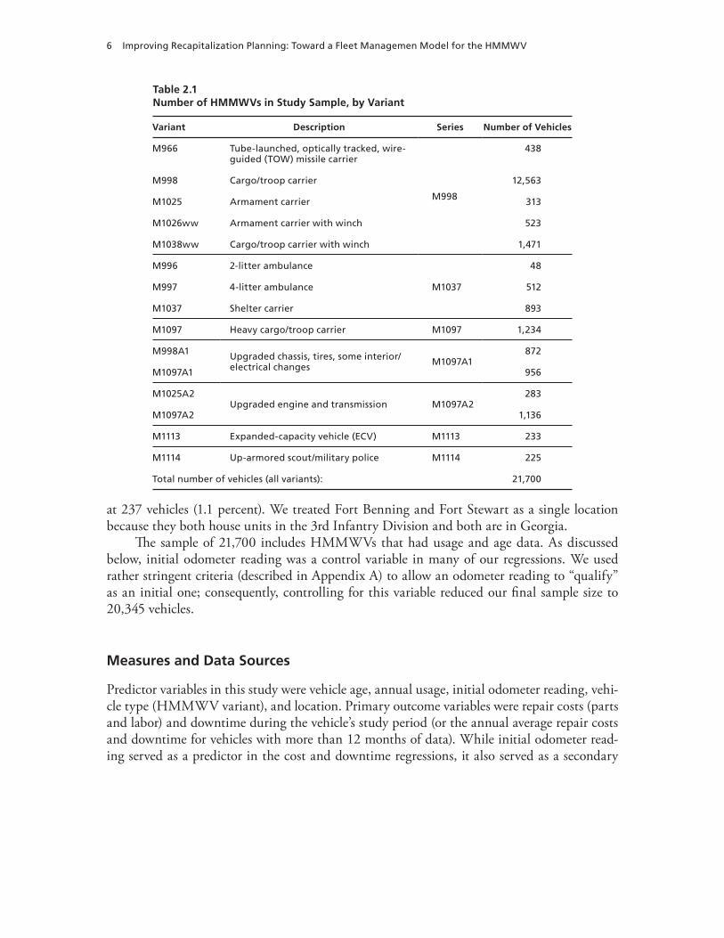
Table 2.1 lists the number of vehicles in the study sample by HMMWV variant. As shown, the basic M998 cargo/troop carrier, with 12,563 vehicles, made up nearly 58 percent of the study sample. The next largest group, with 1,471 vehicles (equal to 6.8 percent), was the M1038, the basic cargo/troop carrier with winch. The smallest group, at 48 vehicles (0.2 per-cent) was the M996 two-litter ambulance variant.

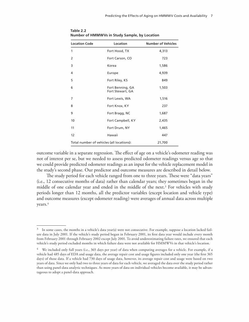
The sample of HMMWVs was spread across 12 different geographic locations as indicated in Table 2.2. As can be seen, Europe and Fort Hood had the largest concentrations at, respec-tively, 4,939 (22.8 percent) and 4,313 (19.9 percent). Fort Knox had the smallest concentration

1 We obtained information on NMC repairs from the EDA; as mentioned previously, the EDA archives daily reports from SAMS-2 on NMC vehicles. Because it compiles daily SAMS reports, the EDA generally does not include NMC repairs concluded between daily report submissions.2 Ideally, this analysis should include all repairs, but vehicle-level data are currently available only for NMC repairs. As noted below, parts used for NMC repairs account for about 20 percent of total parts costs. In the vehicle replacement model, we scale up repair costs to account for other types of repairs, and we vary our assumptions on how non-EDA repair costs are related to age as part of our sensitivity analysis.

6 Improving Recapitalization Planning: Toward a Fleet Managemen Model for the HMMWV

Table 2.1Number of HMMWVs in Study Sample, by Variant

Variant Description Series Number of Vehicles

M966 Tube-launched, optically tracked, wire-guided (TOW) missile carrier

M998

438

M998 Cargo/troop carrier 12,563

M1025 Armament carrier 313

M1026ww Armament carrier with winch 523

M1038ww Cargo/troop carrier with winch 1,471

M996 2-litter ambulance

M1037

48

M997 4-litter ambulance 512

M1037 Shelter carrier 893

M1097 Heavy cargo/troop carrier M1097 1,234

M998A1 Upgraded chassis, tires, some interior/electrical changes M1097A1

872

M1097A1 956

M1025A2Upgraded engine and transmission M1097A2

283

M1097A2 1,136

M1113 Expanded-capacity vehicle (ECV) M1113 233

M1114 Up-armored scout/military police M1114 225

Total number of vehicles (all variants): 21,700

at 237 vehicles (1.1 percent). We treated Fort Benning and Fort Stewart as a single location because they both house units in the 3rd Infantry Division and both are in Georgia.

The sample of 21,700 includes HMMWVs that had usage and age data. As discussed below, initial odometer reading was a control variable in many of our regressions. We used rather stringent criteria (described in Appendix A) to allow an odometer reading to “qualify” as an initial one; consequently, controlling for this variable reduced our final sample size to 20,345 vehicles.

Measures and Data Sources

Predictor variables in this study were vehicle age, annual usage, initial odometer reading, vehi-cle type (HMMWV variant), and location. Primary outcome variables were repair costs (parts and labor) and downtime during the vehicle’s study period (or the annual average repair costs and downtime for vehicles with more than 12 months of data). While initial odometer read-ing served as a predictor in the cost and downtime regressions, it also served as a secondary

Predicting the Effects of Aging on HMMWV Costs and Availability 7

Table 2.2Number of HMMWVs in Study Sample, by Location

Location Code Location Number of Vehicles

1 Fort Hood, TX 4,313

2 Fort Carson, CO 723

3 Korea 1,586

4 Europe 4,939

5 Fort Riley, KS 849

6 Fort Benning, GAFort Stewart, GA

1,503

7 Fort Lewis, WA 1,516

8 Fort Knox, KY 237

9 Fort Bragg, NC 1,687

10 Fort Campbell, KY 2,435

11 Fort Drum, NY 1,465

12 Hawaii 447

Total number of vehicles (all locations): 21,700

outcome variable in a separate regression. The effect of age on a vehicle’s odometer reading was not of interest per se, but we needed to assess predicted odometer readings versus age so that we could provide predicted odometer readings as an input for the vehicle replacement model in the study’s second phase. Our predictor and outcome measures are described in detail below.

The study period for each vehicle ranged from one to three years. These were “data years” (i.e., 12 consecutive months of data) rather than calendar years; they sometimes began in the middle of one calendar year and ended in the middle of the next.3 For vehicles with study periods longer than 12 months, all the predictor variables (except location and vehicle type) and outcome measures (except odometer reading) were averages of annual data across multiple years.4

3 In some cases, the months in a vehicle’s data year(s) were not consecutive. For example, suppose a location lacked fail-ure data in July 2001. If the vehicle’s study period began in February 2001, its first data year would include every month from February 2001 through February 2002 except July 2001. To avoid underestimating failure rates, we ensured that each vehicle’s study period excluded months in which failure data were not available for HMMWVs in that vehicle’s location.4 We included only full years (i.e., 365 days per year) of data when computing averages for a vehicle. For example, if a vehicle had 485 days of EDA and usage data, the average repair cost and usage figures included only one year (the first 365 days) of those data. If a vehicle had 730 days of usage data, however, its average repair cost and usage were based on two years of data. Since we only had two to three years of data for each vehicle, we averaged the data over the study period rather than using panel-data analytic techniques. As more years of data on individual vehicles become available, it may be advan-tageous to adopt a panel-data approach.

8 Improving Recapitalization Planning: Toward a Fleet Managemen Model for the HMMWV

Age

We calculated vehicle age by subtracting the vehicle’s year of manufacture (YOM) from each year of the vehicle’s study period and averaging the differences. Thus, for example, if a vehicle’s study period contained data from 1999, 2000, and 2001 and the vehicle’s YOM was 1988, then Age1999 = 1999 – 1988 = 11, Age2000 = 2000 – 1988 = 12, and Age2001 = 2001 – 1988 = 13. Averaging these results then yielded a vehicle age of 12.5

We obtained YOM data for most HMMWVs in the study from The Army Maintenance Management System (TAMMS) Equipment Database (TEDB) within LIDB.6 We mean cen-tered the age variable to address multi-collinearity problems that can arise when first-order and higher-order (e.g., age and age-squared) terms are included in the same regression (Aiken, West, and Reno, 1991). Mean centering involved transforming the age variable by subtracting the mean HMMWV age for the sample.

Annual Usage

We computed the average annual usage (miles traveled) per vehicle from monthly odometer readings. Like the manufacture dates, odometer readings by serial number came from the TEDB within LIDB. However, many monthly readings were missing, and some had errors, such as missing decimal points. We therefore filtered odometer readings to improve the qual-ity of the data before calculating usage. The criteria used to “weed out” odometer readings for this purpose were not as strict as the criteria used to select a vehicle’s initial odometer reading (see below), as the differences between consecutive odometer readings, rather than the abso-lute odometer readings, were the values of interest in this case. Our filtering process therefore focused on checking consecutive odometer readings for each vehicle. If month n + 1 had a smaller reading than did month n, we treated the month n + 1 reading as a missing data point. Similarly, we treated the month n + 1 reading as a missing value if it exceeded the month n reading by more than 3,000 miles. (Appendix A shows how this cutoff compared to others we tried.)

After filtering the odometer readings, we calculated the usage for month n by subtract-ing the odometer reading for month n from the odometer reading for month n + 1. We then used an imputation technique to substitute approximate values for missing monthly usage.7 If, after imputation, all monthly usage values in a data year were non-missing, we summed the monthly usage values for that data year. If one or more monthly usage values were still missing despite imputation,8 we computed usage during the data year by subtracting the vehicle’s mini-

5 We did not have information on component replacement history. Because repairs had been made before the study period, some components of each vehicle could have been newer than the vehicle itself.6 Because the HMMWV has a clear correspondence between the sequence of manufacture dates and the sequence of serial numbers (see Appendix A), we were able to correct inaccurate manufacture dates and deduce those that were missing from TEDB.7 As in related studies (Peltz et al., 2004a and 2004b), when a vehicle was missing a usage reading for a particular month, we replaced that missing value with the mean usage of other vehicles in the same company during that month. This imputa-tion technique is known as mean substitution.8 Occasionally, all vehicles in a company had missing usage during a particular month. In that case, mean substitution still left vehicles with a missing value.

Predicting the Effects of Aging on HMMWV Costs and Availability 9

mum odometer reading from its maximum reading during that year. Once we determined annual usage—through either the first approach or the second—for all of a vehicle’s data years, we averaged those figures to obtain the vehicle’s average annual usage.

Vehicle Type

We included a set of 14 dummy variables to control for the effects of differences among the 15 HMMWV variants (we used the M998 as the referent variant). Because of differences in their structures, components, and ways of being used, some variants may have a greater tendency to incur repair costs or take longer to repair than other variants.

Location

We used dummy variables to control for the geographic location of HMMWVs in our sample. We determined each vehicle’s geographic location from the UIC listed with its odometer read-ings in TEDB. A location’s environmental conditions, maintenance practices, training profiles, and command policies may affect vehicle failure rates and downtime. Data on these specific factors were not available, so location served as a proxy for the combined effects of these factors. Table 2.2, shown above, lists the 12 locations and the number of vehicles at each. Because there were 12 locations, we had 11 location dummy variables (the referent was Location 4, Europe).

Odometer Reading

As mentioned previously, monthly odometer readings by serial number came from TEDB within LIDB. We needed a single odometer reading from each vehicle to serve as a dependent variable in one regression (and as a control variable when cost and downtime were the depen-dent variables), so we used the first plausible monthly odometer reading we encountered for each vehicle during its study period. We considered a monthly odometer reading plausible if it (a) did not differ vastly from readings in subsequent months and (b) was not extremely unlikely for the vehicle given the vehicle’s age. Appendix A describes the calculations we made to opera-tionalize those criteria and select plausible odometer readings.

Downtime

EDA data include the number of days that a vehicle is inoperative, or “down,” for each NMC repair. We computed a vehicle’s average annual downtime by summing the down days over the vehicle’s study period and dividing by the number of years in that study period. Of the 20,345 HMMWVs in our final sample, 15,277 (75 percent) were down one or more days during the study period.

EDA-Based Repair Costs

For each HMMWV, we computed average annual repair costs associated with mission-criti-cal failures. Specifically, we summed the NMC repair costs over a vehicle’s study period and

10 Improving Recapitalization Planning: Toward a Fleet Managemen Model for the HMMWV

divided by the number of years in that study period.9 The cost for an individual NMC repair consists of the cost of replacement parts and the cost of the associated labor.

Parts costs. The EDA identified the parts ordered from the supply system for a given repair. Almost all EDA-listed repairs (99.65 percent) involved fewer than 21 parts. However, some repairs had an unusually large number of part orders, perhaps because certain vehicles were serving as the HMMWV equivalent of “hangar queens,” their parts being cannibalized to repair other vehicles. To filter out these extreme cases, our computation of parts costs was based on the 20 most expensive parts ordered for each repair.

The costs of ordered parts came from the Federal Logistics Catalog (FEDLOG) for fiscal year 2003 (FY03).10 The FEDLOG provides the price of each part—defined as the latest acqui-sition cost plus a surcharge to cover the cost of supply system operations—and the credit for returning a broken part that can be repaired at higher echelons.11 For reparable components, we used the net price (or price minus unserviceable credit) as the parts cost; for consum-able components, we used the FEDLOG price as the parts cost (see Appendix A for more information).12

9 Ideally, one would also include costs for the oil and fuel that a vehicle consumed, for scheduled maintenance, and for unscheduled repairs not included in the EDA. However, this information is either not tracked or not readily available on a per-vehicle basis. We investigated the possibility of using data on unscheduled maintenance events from the SDC program operated by AMSAA. The SDC program typically involves manual collection of data for a few hundred vehicles during a fixed period and attempts to capture all parts replaced (i.e., those available in the prescribed load list at the company level and direct support bench and shop stocks, which are not recorded in the supply system and thus are not in the EDA, as well as those provided from supply support activities and the wholesale supply system), as well as the maintenance labor hours associated with each part’s replacement. However, the small sample sizes are less conducive to estimating cost-versus-age relationships, because they tend to have a more limited spread of vehicle ages and because analyses of small samples are subject to greater influence from extreme observations. For example, the annual costs for a vehicle are very high if an expensive component such as an engine or transmission must be replaced, but these events are relatively rare at all vehicle ages. Also, there was very little overlap between recent SDC samples and the EDA data used for this study, so we were unable to get a good estimate of the fraction of repairs captured by SDC that were not included in our EDA data.10 Although changes in prices and credits over time are another way to capture aging costs if components become more expensive to repair or replace as they age, the Army’s credit policy was changing during the study period, making it difficult to compare credits from year to year. Surcharge rates also changed from year to year, so prices do not purely reflect changing acquisition costs.11 In FY03, the Army’s supply management surcharge was 24.1 percent. Under the Single Stock Fund (SSF), the Army completed capitalization of assets in Authorized Stockage Lists (ASLs) into the Army Working Capital Fund (AWCF) in FY03. The surcharge covers the cost of AWCF supply management operations, including inventory management, receipt and issue, transportation, inventory losses, and obsolescence. It does not cover the costs of military personnel who operate supply support activities or who order parts for maintenance activities. (See Department of the Army, 2003.)12 An alternative source of parts cost information is the Operating and Support Management Information System (OSMIS), which provides data on all parts purchased through the AWCF. Although OSMIS gives the best estimate of total parts costs for all types of maintenance and local component repairs, it does not show parts costs associated with individual vehicles. As a result, OSMIS data are more useful for unit-level analyses than for lower levels of analysis. A second problem with these data is that common parts recorded in the system are attributed based on vehicle density within a unit (i.e., pro-portionately) rather than on actual demands for parts. And a third problem is that the AWCF point of sale changed twice in recent years, resulting in the inclusion of more parts-demand data over time. This could lead to spurious aging effects.

Predicting the Effects of Aging on HMMWV Costs and Availability 11

Labor costs. Maintenance allocation charts, or MACs, and SDC records provided esti-mates of the labor hours needed to remove and replace parts.13 MACs are typically developed as part of the technical data associated with a vehicle; they specify the standard number of labor hours associated with each maintenance and repair action. SDC data, in contrast, pro-vide actual labor hours for each part replaced based on the sample of vehicles tracked. When we had SDC labor hours for a part, we used them to determine the labor hours for parts replaced during a repair. When we did not have SDC labor hours for a part, we used MAC labor hours, if available. Between the two sources, we had labor hours for 96 percent of the HMMWV parts in the EDA data.14

Cost factors for military labor hours by rank came from SAFM-CE and TACOM. The weighted average hourly rate, $31.54, was based on the proportions of soldiers in ranks E3 through E8 used to maintain the Family of Medium Tactical Vehicles. We increased this figure by 40 percent (to $44.16 per hour) to account for indirect productive time.15 However, this adjustment probably does not fully account for the indirect costs of maintaining vehicles, such as the costs of facilities, equipment and tools, parts inventories, information systems, training, and supervision. As vehicle fleets age, it becomes more difficult to predict how many and what types of resources will be needed to maintain the fleet at an acceptable level of readi-ness. Consequently, maintenance operations have to stockpile more of these resources to sup-port an older fleet. If indirect costs increase with fleet age, the slope of our cost regression may be underestimated, and optimal replacement ages may be lower.

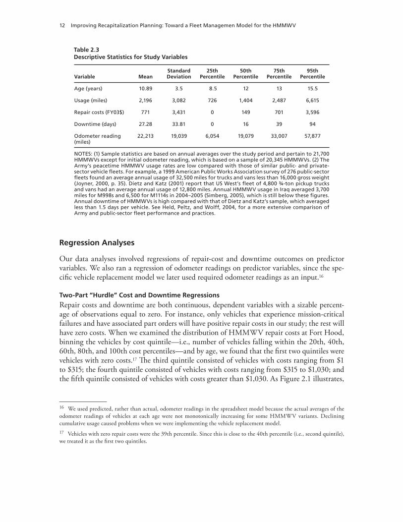
Of the 20,345 HMMWVs in our final sample, 13,415 had NMC repair costs greater than zero during the period in which they were observed. Table 2.3 shows descriptive statistics for all of the major variables in our regressions.

13 MACs are based on part descriptions or part numbers instead of National Stock Numbers (NSNs). To facilitate the matching of labor hours to NSNs, the U.S. Army Tank-automotive and Armaments Command (TACOM) provided a list of maintenance labor hours that could be identified from MACs for the top 300 cost-driving parts associated with HMMWVs in OSMIS.14 Our estimated labor costs using this technique were about 20 percent of parts costs. This percentage is low compared with that for other vehicle maintenance operations. For example, a benchmarking study of the maintenance costs of con-struction equipment (Sutton, 2005a, 2005b) found that parts costs ranged from 23 to 60 percent of total maintenance costs, with the owners of the largest fleets (by replacement value) tending to have the smallest percentage of parts costs. In contrast, our parts costs were about 83 percent of total costs. Thus, we may not have captured all of the maintenance man-hours or the indirect costs that should go into the fully burdened cost of mechanic labor.15 Indirect productive time is defined as the time associated with duties the mechanic must perform relating to a mainte-nance or repair action aside from “wrench-turning” tasks. It includes maintenance administration; training; delays; support equipment operation; travel time; shop/area cleaning; maintaining and cleaning tools, shop sets, and outfits; tool room and storage activities; and shop supply operations. It is typically assumed to be 40 percent of direct productive hours for field-level maintenance. See U.S. Army Force Management Support Agency, 2005.

12 Improving Recapitalization Planning: Toward a Fleet Managemen Model for the HMMWV

Table 2.3Descriptive Statistics for Study Variables

Variable MeanStandard Deviation

25th Percentile

50th Percentile

75th Percentile

95th Percentile

Age (years) 10.89 3.5 8.5 12 13 15.5

Usage (miles) 2,196 3,082 726 1,404 2,487 6,615

Repair costs (FY03$) 771 3,431 0 149 701 3,596

Downtime (days) 27.28 33.81 0 16 39 94

Odometer reading (miles)

22,213 19,039 6,054 19,079 33,007 57,877

NOTES: (1) Sample statistics are based on annual averages over the study period and pertain to 21,700 HMMWVs except for initial odometer reading, which is based on a sample of 20,345 HMMWVs. (2) The Army’s peacetime HMMWV usage rates are low compared with those of similar public- and private-sector vehicle fleets. For example, a 1999 American Public Works Association survey of 276 public-sector fleets found an average annual usage of 32,500 miles for trucks and vans less than 16,000 gross weight (Joyner, 2000, p. 35). Dietz and Katz (2001) report that US West’s fleet of 4,800 ¾-ton pickup trucks and vans had an average annual usage of 12,800 miles. Annual HMMWV usage in Iraq averaged 3,700 miles for M998s and 6,500 for M1114s in 2004–2005 (Simberg, 2005), which is still below these figures. Annual downtime of HMMWVs is high compared with that of Dietz and Katz’s sample, which averaged less than 1.5 days per vehicle. See Held, Peltz, and Wolff, 2004, for a more extensive comparison of Army and public-sector fleet performance and practices.

Regression Analyses

Our data analyses involved regressions of repair-cost and downtime outcomes on predictor variables. We also ran a regression of odometer readings on predictor variables, since the spe-cific vehicle replacement model we later used required odometer readings as an input.16

Two-Part “Hurdle” Cost and Downtime Regressions

Repair costs and downtime are both continuous, dependent variables with a sizable percent-age of observations equal to zero. For instance, only vehicles that experience mission-critical failures and have associated part orders will have positive repair costs in our study; the rest will have zero costs. When we examined the distribution of HMMWV repair costs at Fort Hood, binning the vehicles by cost quintile—i.e., number of vehicles falling within the 20th, 40th, 60th, 80th, and 100th cost percentiles—and by age, we found that the first two quintiles were vehicles with zero costs.17 The third quintile consisted of vehicles with costs ranging from $1 to $315; the fourth quintile consisted of vehicles with costs ranging from $315 to $1,030; and the fifth quintile consisted of vehicles with costs greater than $1,030. As Figure 2.1 illustrates,

16 We used predicted, rather than actual, odometer readings in the spreadsheet model because the actual averages of the odometer readings of vehicles at each age were not monotonically increasing for some HMMWV variants. Declining cumulative usage caused problems when we were implementing the vehicle replacement model.17 Vehicles with zero repair costs were the 39th percentile. Since this is close to the 40th percentile (i.e., second quintile), we treated it as the first two quintiles.

Predicting the Effects of Aging on HMMWV Costs and Availability 13

Figure 2.1HMMWV Costs at Fort Hood, Binned by Repair Cost and Age

100

1514.51413.51312.51211.51110.5109.598.587.576.565.554.543.532.52 16

Vehicle age (years)

Perc

enta

ge

of

veh

icle

s in

ag

e g

rou

p

>$1,030 $0$1 to $315$315 to $1,030

80

60

40

20

0

RAND TR464-2.1

the number of vehicles with zero costs was substantial but decreased with age, and the number of vehicles in the other cost quintiles (particularly the top two) increased with age.

Just as NMC repair costs are positive only for vehicles that have mission-critical failures and associated part orders, downtime is positive only for vehicles that are inoperative for one or more days; otherwise, downtime is zero. Dependent variables with these characteristics are considered “limited dependent variables,” meaning that the values they can take are con-strained. Our analysis had to address these variables accordingly.

Limited dependent variables are also found in the field of health economics. One outcome variable that exhibits characteristics similar to those of repair costs and downtime, for example, is “medical expenditures” from hospitalization, since the only individuals who will have hospi-tal bills are those who are hospitalized. Prior health-economics studies typically have used two-part “hurdle” regressions to model effects on limited dependent variables (e.g., Kapur, Young, and Murata, 2000; Liu, Long, and Dowling, 2003; Sturm, 2000).18 In these studies, the first part of the procedure entails a logistic regression model in which the dependent variable is a binary measure of whether or not a patient has a non-zero healthcare expenditure. The second part involves an ordinary least squares (OLS) regression in which the dependent variable is the amount of the expenditure, so long as the expenditure is non-zero. The probability predictions

18 The procedure has also been used in other fields, with such dependent variables as political contributions (Apollonio and La Raja, 2004) and the number of cigarettes smoked daily (Lundborg and Lindgren, 2004).

14 Improving Recapitalization Planning: Toward a Fleet Managemen Model for the HMMWV

from the first part of the procedure are then multiplied by the expenditure predictions from the second part to determine expected expenditures.19

In the current study, we used the two-part technique to assess the effects of vehicle age and other predictors on the repair costs and downtime of HMMWVs. For each regression, we began with a full model, including higher-order age and usage terms, and then reduced the model using sequential type III sum of squares tests.20 The structure of each full-model regres-sion equation (prior to reduction) was as follows:

Dependent variable = location 1 lo0 1 2β β β+ +( ) ( ccation 2 location 3

location 53

4

) ( )

( )

+

+ +

β

β ββ β β5 6 7location 6 location 7 location( ) ( ) (+ + 88

location 9 location 10 lo8 9 10

)

( ) ( ) (+ + +β β β ccation 11

location 12 variant11 12

)

( ) (+ +β β 11 variant 2 variant 3

var13 14

15

) ( ) ( )

(

+ +

+

β β

β iiant 4 variant 5 variant 616 17 18) ( ) ( ) (+ + +β β β vvariant 7

variant 8 variant 919 20

)

( ) ( )+ +β β ++ +

+

β β

β21 22

23

variant 10 variant 11

var

( ) ( )

( iiant 12 variant 13 variant 1424 25) ( ) ( )+ +

+

β β

( ) ( ) (β β β26 272

28odometer odometer odometer+ + 3329

302

313

3

usage

usage usage

) ( )

( ) ( )

+

+ + +

β

β β β 22 332

343

35

age age age

usage ag

( ) ( ) ( )

(

+ +

+ ×

β β

β

4

ee usage age usage age

o36

237

2

38

) ( ) ( )

(

+ × + ×

+

β β

β ddometer age odometer age

odom39

2

40

× + ×

+

) ( )

(

β

β eeter age odometer usage

odome

241

42

× + ×

+

) ( )

(

β

β tter usage odometer usage243

2× + ×) ( )β

where locations 1 through 12 are the dummy variables representing 11 of the 12 locations in the study, and variants 1 through 14 are the dummy variables representing 14 of the 15 HMMWV variants in the study. The equation did not include dummy variables for location 4 (Europe) and the M998 variant since those were referent categories. The cost and downtime regressions

19 If the dependent variable in the second part of the model has been transformed logarithmically (i.e., log of expendi-tures), simple retransformations of the predicted values (i.e., exponential of predicted expenditures) may be statistically biased. That is, the simple retransformations tend to be reasonable estimates of the median of the original distribution, but not the mean. The approach we used to address this bias was Duan’s (1983) smearing estimate. Calculated as the mean of the exponential of residuals, Duan’s smearing estimate is a factor by which one can multiply the retransformed predicted values to correct for the bias (Diehr et al., 1999; Pasta and Cisternas, 2003). 20 We sequentially eliminated statistically insignificant predictors from the model except when those predictors were lower-order terms (e.g., age) whose higher-order terms (e.g., age squared) were statistically significant.

Predicting the Effects of Aging on HMMWV Costs and Availability 15

included clustering on location x variant (the product of the two dummy variables) to account for the possibility that the two variables in combination could affect the dependent variable.21

For the repair-cost logistic regression, the dependent variable was a binary variable equal-ing one if a vehicle’s average repair costs were positive and equaling zero otherwise. For the repair-cost OLS regression, the dependent variable was ln(vehicle repair costs). Similarly, for the downtime logistic regression, the dependent variable was a binary variable equaling one if a vehicle had positive average downtime and equaling zero otherwise. For the downtime OLS regression, the dependent variable was ln(vehicle downtime).

In the cost and downtime regressions, we rescaled the usage and odometer variables, dividing each by 100 (so that one unit change in usage or odometer would be equivalent to 100 miles). We did this to facilitate interpretation of the regression coefficients.

OLS Odometer Regression. In addition to running regressions of cost versus age and availability versus age, we ran regressions of odometer readings versus age. One of the key inputs for the vehicle replacement spreadsheet model (discussed in Chapter Four) was the set of odometer readings for vehicles of different ages. Because we were predicting a single odometer reading for each vehicle, our odometer regression used cross-sectional data rather than averag-ing multiple years of data. The regression equation, which excluded dummy variables for the referent categories, location 4 (Europe) and the M998 variant, was as follows:

ln vehicle odometer reading locatio0 1( ) ( nn 1 location 2 location 3loc

2 3

4

) ( ) ( )( aation 5 location 6 location 75 6

7

) ( ) ( ) (( ) ( ) (location 8 location 9 location 108 9 ))

( ) ( ) ( 10 11 12location 11 location 12 vaariant 1variant 2 variant 313 14

)( ) ( ) 115

16 17

variant 4variant 5 variant

( )( ) ( 66 variant 7variant 8 vari

18

19 20

) ( )( ) ( aant 9 variant 10variant 11

21

22 2

) ( )( ) 33 24

25

variant 12 variant 13variant

( ) ( )( 14 age age age26 27 28

2 3) ( ) ( ) ( )

21 Clustering adjusts the standard errors to account for the possibility that the error terms are not independent within “clusters,” or groups of observations with the same attribute(s). (See, for example, Primo, Jacobsmeier, and Milyo, 2006; or Begg and Parides, 2003.) We used SAS® procedure SURVEYREG to implement clustering in the OLS regressions (Ber-glund, 2002) and a SAS® macro developed by Dan McCaffrey and Claude Setodji of RAND to implement clustering in the logistic regressions.

17

CHAPTER THREE

Estimation Results

In this chapter, we present a series of plots derived from our cost, availability, and odometer-reading regressions. Most of these plots pertain specifically to the M998, the most prevalent variant in our sample (the regression tables, which show results for all variants, appear in Appendix B). We found age to have positive effects on the probabilities that repair costs and downtime were greater than zero and on the magnitudes of repair costs and downtime when their values were positive.1

Cost Versus Age

Figure 3.1 illustrates the annual probability of incurring repair costs (i.e., probability that cost is greater than zero) as a function of vehicle age when usage is held constant at 2,000 miles per year. (Odometer readings were set at the predicted values based on the odometer-versus-age regression.) This plot corresponds to the first part of our two-part hurdle regressions for repair costs associated with mission-critical failures. Older vehicles showed greater probabilities of having repair costs. For example, in Europe (our referent location), vehicles aged 1 to 5 years had a 20 to 30 percent likelihood of incurring NMC repair costs in a year, whereas vehicles aged 13 to 15 years had likelihoods closer to 68 percent. The aging effect was curvilinear, with a significant quadratic age term and a smaller but significant cubic age term (see Appendix B). The curvilinear effect indicates that the probability of incurring costs increased with age; how-ever, that increase was steeper for younger vehicles than for older vehicles. It is important to note that the tail region of the curve is characterized by more uncertainty than is the middle region, given that our sample had very few HMMWVs older than 15 years.

The probability that a vehicle had positive NMC repair costs varied by location. For example, vehicles in Korea tended to have the highest probabilities, ranging from 65 to 95 percent throughout their histories. Vehicles at Fort Bragg, by contrast, experienced the lowest probabilities, ranging from around 10 percent in their early years to around 50 percent near age 14. These variations by location may stem from differences in operating conditions (e.g., on-road versus off-road usage, terrain, and weather), differences in maintenance practices and personnel skill levels, or other, unobserved differences.

1 Although our analysis focused primarily on the aging effects illustrated in this chapter, Appendix B provides a plot showing the effect of usage on repair costs.

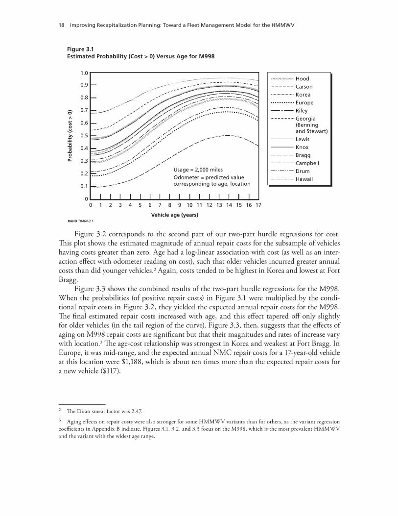
18 Improving Recapitalization Planning: Toward a Fleet Management Model for the HMMWV

Figure 3.1Estimated Probability (Cost > 0) Versus Age for M998

0.9

0.3

0.2

0.1

1.0

1716210

Vehicle age (years)

Pro

bab

ility

(co

st >

0)

0

0.8

0.7

0.6

0.5

0.4

RAND TR464-3.1

1514

Usage = 2,000 milesOdometer = predicted valuecorresponding to age, location

131211109876543

Hood

Carson

Korea

Europe

Riley

Georgia(Benningand Stewart)

Lewis

Knox

Bragg

Campbell

Drum

Hawaii

Figure 3.2 corresponds to the second part of our two-part hurdle regressions for cost. This plot shows the estimated magnitude of annual repair costs for the subsample of vehicles having costs greater than zero. Age had a log-linear association with cost (as well as an inter-action effect with odometer reading on cost), such that older vehicles incurred greater annual costs than did younger vehicles.2 Again, costs tended to be highest in Korea and lowest at Fort Bragg.

Figure 3.3 shows the combined results of the two-part hurdle regressions for the M998. When the probabilities (of positive repair costs) in Figure 3.1 were multiplied by the condi-tional repair costs in Figure 3.2, they yielded the expected annual repair costs for the M998. The final estimated repair costs increased with age, and this effect tapered off only slightly for older vehicles (in the tail region of the curve). Figure 3.3, then, suggests that the effects of aging on M998 repair costs are significant but that their magnitudes and rates of increase vary with location.3 The age-cost relationship was strongest in Korea and weakest at Fort Bragg. In Europe, it was mid-range, and the expected annual NMC repair costs for a 17-year-old vehicle at this location were $1,188, which is about ten times more than the expected repair costs for a new vehicle ($117).

2 The Duan smear factor was 2.47.3 Aging effects on repair costs were also stronger for some HMMWV variants than for others, as the variant regression coefficients in Appendix B indicate. Figures 3.1, 3.2, and 3.3 focus on the M998, which is the most prevalent HMMWV and the variant with the widest age range.

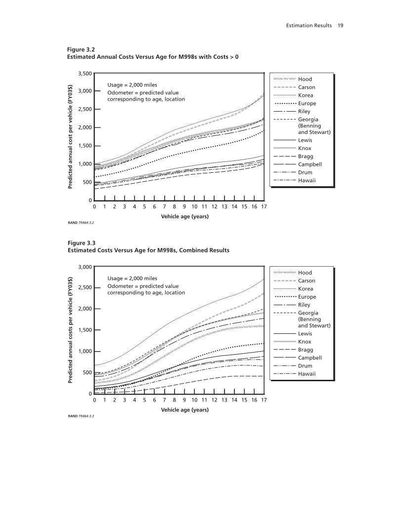
Estimation Results 19

Figure 3.2Estimated Annual Costs Versus Age for M998s with Costs > 0

1,500

1,000

500

3,500

1716210

Vehicle age (years)

Pred

icte

d a

nn

ual

co

st p

er v

ehic

le (

FY03

$)

0

3,000

2,500

2,000

RAND TR464-3.2

1514131211109876543

Hood

Carson

Korea

Europe

Riley

Georgia(Benningand Stewart)

Lewis

Knox

Bragg

Campbell

Drum

Hawaii

Usage = 2,000 milesOdometer = predicted valuecorresponding to age, location

Figure 3.3Estimated Costs Versus Age for M998s, Combined Results

1,500

1,000

500

3,000

1716210

Vehicle age (years)

Pred

icte

d a

nn

ual

co

sts

per

veh

icle

(FY

03$)

0

2,500

2,000

RAND TR464-3.3

1514131211109876543

Hood

Carson

Korea

Europe

Riley

Georgia(Benningand Stewart)

Lewis

Knox

Bragg

Campbell

Drum

Hawaii

Usage = 2,000 milesOdometer = predicted valuecorresponding to age, location

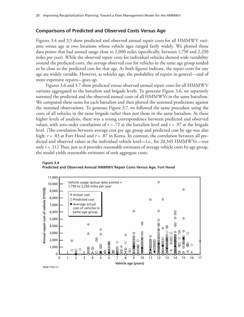
20 Improving Recapitalization Planning: Toward a Fleet Management Model for the HMMWV

Comparisons of Predicted and Observed Costs Versus Age

Figures 3.4 and 3.5 show predicted and observed annual repair costs for all HMMWV vari-ants versus age at two locations whose vehicle ages ranged fairly widely. We plotted those data points that had annual usage close to 2,000 miles (specifically, between 1,750 and 2,250 miles per year). While the observed repair costs for individual vehicles showed wide variability around the predicted costs, the average observed cost for vehicles in the same age group tended to be close to the predicted cost for that age. As both figures indicate, the repair costs for any age are widely variable. However, as vehicles age, the probability of repairs in general—and of more expensive repairs—goes up.

Figures 3.6 and 3.7 show predicted versus observed annual repair costs for all HMMWV variants aggregated to the battalion and brigade levels. To generate Figure 3.6, we separately summed the predicted and the observed annual costs of all HMMWVs in the same battalion. We computed these sums for each battalion and then plotted the summed predictions against the summed observations. To generate Figure 3.7, we followed the same procedure using the costs of all vehicles in the same brigade rather than just those in the same battalion. At these higher levels of analysis, there was a strong correspondence between predicted and observed values, with zero-order correlations of r = .72 at the battalion level and r = .97 at the brigade level. (The correlation between average cost per age group and predicted cost by age was also high: r = .83 at Fort Hood and r = .87 in Korea. In contrast, the correlation between all pre-dicted and observed values at the individual vehicle level—i.e., for 20,345 HMMWVs—was only r = .11.) Thus, just as it provides reasonable estimates of average vehicle costs by age group, the model yields reasonable estimates of unit aggregate costs.

Figure 3.4Predicted and Observed Annual HMMWV Repair Costs Versus Age, Fort Hood

9,000

8,000

Vehicle usage (actual data points) =1,750 to 2,250 miles per year

7,000

6,000

5,000

4,000

3,000

2,000

1,000

11,000

171643210

Vehicle age (years)

An

nu

al r

epai

r co

st o

f ve

hic

le (

FY03

$)

0

10,000

RAND TR464-3.4

15141312111098765

Actual costPredicted costAverage actualcost of vehicles insame age group

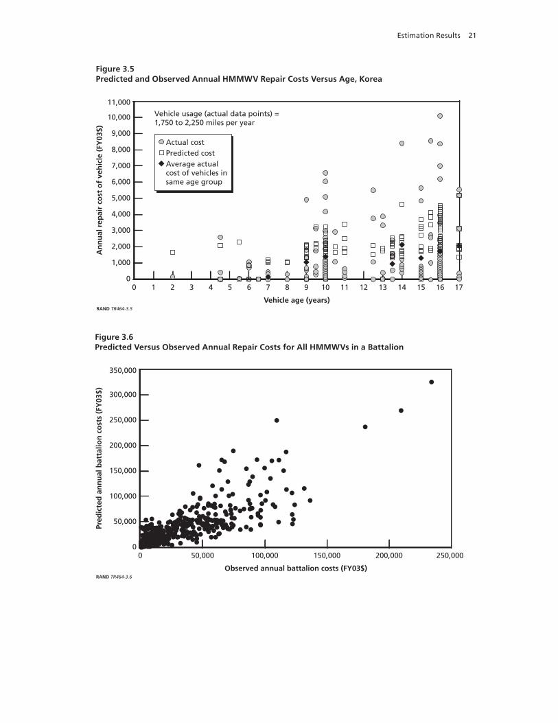
Estimation Results 21

Figure 3.5Predicted and Observed Annual HMMWV Repair Costs Versus Age, Korea

9,000

8,000

Vehicle usage (actual data points) =1,750 to 2,250 miles per year

7,000

6,000

5,000

4,000

3,000

2,000

1,000

11,000

171643210

Vehicle age (years)

An

nu

al r

epai

r co

st o

f ve

hic

le (

FY03

$)

0

10,000

RAND TR464-3.5

15141312111098765

Actual costPredicted costAverage actualcost of vehicles insame age group

Figure 3.6Predicted Versus Observed Annual Repair Costs for All HMMWVs in a Battalion

300,000

250,000

200,000

150,000

100,000

50,000

350,000

250,000100,00050,0000

Observed annual battalion costs (FY03$)

Pred

icte

d a

nn

ual

bat

talio

n c

ost

s (F

Y03

$)

0

RAND TR464-3.6

200,000150,000

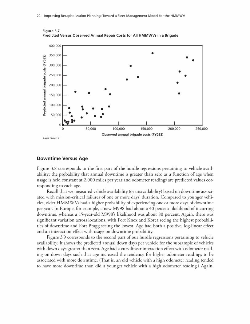
22 Improving Recapitalization Planning: Toward a Fleet Management Model for the HMMWV

Figure 3.7Predicted Versus Observed Annual Repair Costs for All HMMWVs in a Brigade

350,000

300,000

250,000

200,000

150,000

100,000

50,000

400,000

250,000100,00050,0000

Observed annual brigade costs (FY03$)

Pred

icte

d a

nn

ual

bri

gad

e co

sts

(FY

03$)

0

RAND TR464-3.7

200,000150,000

Downtime Versus Age

Figure 3.8 corresponds to the first part of the hurdle regressions pertaining to vehicle avail-ability: the probability that annual downtime is greater than zero as a function of age when usage is held constant at 2,000 miles per year and odometer readings are predicted values cor-responding to each age.

Recall that we measured vehicle availability (or unavailability) based on downtime associ-ated with mission-critical failures of one or more days’ duration. Compared to younger vehi-cles, older HMMWVs had a higher probability of experiencing one or more days of downtime per year. In Europe, for example, a new M998 had about a 40 percent likelihood of incurring downtime, whereas a 15-year-old M998’s likelihood was about 80 percent. Again, there was significant variation across locations, with Fort Knox and Korea seeing the highest probabili-ties of downtime and Fort Bragg seeing the lowest. Age had both a positive, log-linear effect and an interaction effect with usage on downtime probability.

Figure 3.9 corresponds to the second part of our hurdle regressions pertaining to vehicle availability. It shows the predicted annual down days per vehicle for the subsample of vehicles with down days greater than zero. Age had a curvilinear interaction effect with odometer read-ing on down days such that age increased the tendency for higher odometer readings to be associated with more downtime. (That is, an old vehicle with a high odometer reading tended to have more downtime than did a younger vehicle with a high odometer reading.) Again,

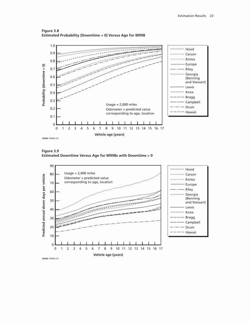
Estimation Results 23

Figure 3.8Estimated Probability (Downtime > 0) Versus Age for M998

0.9

0.3

0.2

0.1

1.0

1716210

Vehicle age (years)

Pro

bab

ility

(d

ow

nti

me

> 0

)

0

0.8

0.7

0.6

0.5

0.4

RAND TR464-3.8

1514

Usage = 2,000 milesOdometer = predicted valuecorresponding to age, location

131211109876543

Hood

Carson

Korea

Europe

Riley

Georgia(Benningand Stewart)

Lewis

Knox

Bragg

Campbell

Drum

Hawaii

Figure 3.9Estimated Downtime Versus Age for M998s with Downtime > 0

30

20

10

90

1716210

Vehicle age (years)

Pred

icte

d a

nn

ual

do

wn

day

s p

er v

ehic

le

0

80

70

60

50

40

RAND TR464-3.9

1514

Usage = 2,000 milesOdometer = predicted valuecorresponding to age, location

131211109876543

Hood

Carson

Korea

Europe

Riley

Georgia(Benningand Stewart)

Lewis

Knox

Bragg

Campbell

Drum

Hawaii

24 Improving Recapitalization Planning: Toward a Fleet Management Model for the HMMWV

there were location effects. Vehicles with the highest number of down days tended to be in Korea or at Fort Knox; vehicles with the lowest number of down days tended to be at Fort Drum.

Figure 3.10 presents the combined results of the two-part hurdle regressions for availabil-ity. Here the probabilities of incurring downtime (shown in Figure 3.8) are multiplied by the conditional days of downtime (shown in Figure 3.9) to yield the expected days of downtime as a function of vehicle age. Figure 3.10 illustrates that the effects of aging on vehicle avail-ability are significant. For example, a new M998 experiences an average of about 6 to 33 days of downtime per year, depending on location; whereas a 15-year-old M998 experiences about 25 to 72 days of downtime per year. Vehicles located in Korea and at Fort Knox typically experienced a higher number of down days, and those at Fort Bragg and Fort Drum typically experienced fewer.

Odometer Reading Versus Age

Figure 3.11 is a plot derived from the regression of odometer readings, or, more specifically, a plot of predicted odometer readings versus vehicle age. As one might expect, older vehicles had higher predicted odometer readings. The effect of age was log-cubic, suggesting that vehicle usage (i.e., change in odometer reading) tapered off a bit around age 10 but then increased for older vehicles. Recall that we used predicted odometer readings by age as an input to the

Figure 3.10Estimated Downtime Versus Age for M998s, Combined Results

30

20

10

90

1716210

Vehicle age (years)

Pred

icte

d a

nn

ual

do

wn

day

s p

er v

ehic

le

0

80

70

60

50

40

RAND TR464-3.10

1514

Usage = 2,000 milesOdometer = predicted valuecorresponding to age, location

131211109876543

Hood

Carson

Korea

Europe

Riley

Georgia(Benningand Stewart)

Lewis

Knox

Bragg

Campbell

Drum

Hawaii

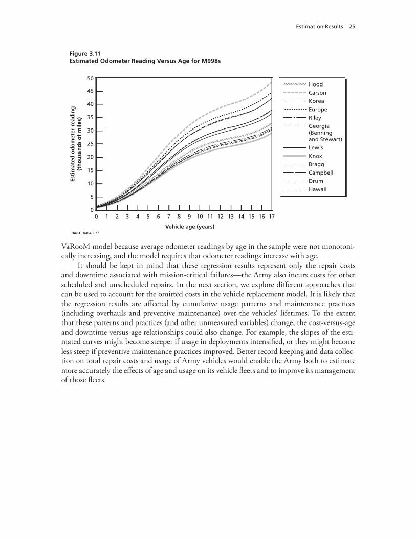
Estimation Results 25

Figure 3.11Estimated Odometer Reading Versus Age for M998s

45

15

10

5

50

1716210

Vehicle age (years)

Esti

mat

ed o

do

met

er r

ead

ing

(th

ou

san

ds

of

mile

s)

0

40

35

30

25

20

RAND TR464-3.11

1514131211109876543

Hood

Carson

Korea

Europe

Riley

Georgia(Benningand Stewart)

Lewis

Knox

Bragg

Campbell

Drum

Hawaii

VaRooM model because average odometer readings by age in the sample were not monotoni-cally increasing, and the model requires that odometer readings increase with age.

It should be kept in mind that these regression results represent only the repair costs and downtime associated with mission-critical failures—the Army also incurs costs for other scheduled and unscheduled repairs. In the next section, we explore different approaches that can be used to account for the omitted costs in the vehicle replacement model. It is likely that the regression results are affected by cumulative usage patterns and maintenance practices (including overhauls and preventive maintenance) over the vehicles’ lifetimes. To the extent that these patterns and practices (and other unmeasured variables) change, the cost-versus-age and downtime-versus-age relationships could also change. For example, the slopes of the esti-mated curves might become steeper if usage in deployments intensified, or they might become less steep if preventive maintenance practices improved. Better record keeping and data collec-tion on total repair costs and usage of Army vehicles would enable the Army both to estimate more accurately the effects of age and usage on its vehicle fleets and to improve its management of those fleets.

27

CHAPTER FOUR

Application of the Vehicle Replacement Model

The second part of our study involved running a vehicle replacement model using inputs derived from our regressions and other sources. This model, adapted from the Dietz and Katz (2001) VaRooM vehicle replacement model, helped provide us with insights about optimal replacement and RECAP times for the HMMWV fleet. We selected this model for four main reasons: its inputs and outputs are applicable to Army vehicle replacement decisions, it is adapt-able (we were able to modify it in order to assess RECAP alternatives, for example), its Micro-soft Excel® platform is widely available, and it is user friendly enough to serve as an interactive decision support tool for persons with diverse skill sets and experiences. Additionally, VaRooM is particularly well suited to the type of HMMWV data available from Army sources.

VaRooM minimizes cost per mile instead of average annual operating cost (AAOC), which is beneficial because the cost-per-mile metric helps control for possible declining usage of older vehicles. In contrast to the VaRooM model, some models assume that maintenance costs rise at a constant percentage rate over time (e.g., PARIS [East, 2002]), make other restric-tive assumptions about the functional form of costs, or have more-stringent data requirements (such as longer repair histories on individual vehicles).

Originally designed to track a mixture of vehicle types at a telecommunications company, VaRooM employs a spreadsheet format. Below we provide a brief description of the model, explain how we used the regression results described in the previous chapter to derive inputs for the model, and present key parameters of the model.1

Overview of the VaRooM Vehicle Replacement Model

VaRooM allows one to calculate optimal replacement age for each variant of a vehicle (e.g., each HMMWV variant). Figure 4.1 shows a VaRooM worksheet corresponding to the M998. The model segregates vehicles of a given variant by age, calculates each age group’s average operating cost (i.e., cumulative cost/cumulative miles) based on inputs and parameters, and then determines optimal replacement age and optimal cost by minimizing the life-cycle aver-

1 We did not use three of VaRooM’s features: (1) the ability to input information on individual vehicles rather than esti-mated values for large groups of vehicles, (2) a replacement score that can be used to prioritize vehicles for replacement based on their projected cost savings or to allocate a limited vehicle replacement budget, and (3) the ability to determine whether a vehicle that requires an expensive repair should be replaced instead of repaired.

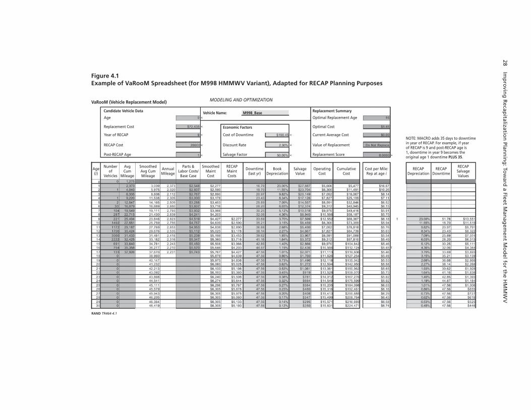
28 Imp

rovin

g R

ecapitalizatio

n Plan

nin

g: To

ward

a Fleet Man

agem

ent M

od

el for th

e HM

MW

V

Figure 4.1Example of VaRooM Spreadsheet (for M998 HMMWV Variant), Adapted for RECAP Planning Purposes

Age(i)

Numberof

Vehicles

AvgCum

Mileage

AnnualMileage

Parts &Labor Costs/Base Case

SmoothedMaintCost

RECAPMaintCosts

Downtime(last yr)

BookDepreciation

SalvageValue

OperatingCost

Replacement Summary

Economic Factors Optimal Cost

Current Average Cost

Value of Replacement

Optimal Replacement Age

Replacement Score

Candidate Vehicle Data Vehicle Name: M998_Base

Replacement Cost

Year of RECAP

RECAP Cost

Age

Post-RECAP Age

Cost of Downtime

Discount Rate

Salvage Factor

CumulativeCost

Cost per Mile:Rep at age i

RECAPDepreciation

NOTE: MACRO adds 35 days to downtimein year of RECAP. For example, if yearof RECAP is 9 and post-RECAP age is1, downtime in year 9 becomes theoriginal age 1 downtime PLUS 35.

RECAPDowntime

RECAPSalvageValues

SmoothedAvg CumMileage

VaRooM (Vehicle Replacement Model) MODELING AND OPTIMIZATION

RAND TR464-4.1

Application of the Vehicle Replacement Model 29

age cost per mile, which in the model is defined as “average cost.” The average cost for a vehicle of age i (ACi ) is computed as

ACi = (CCi + RPC + RCCj + TBi – SVi ) / ACMi

where CCi is the discounted cumulative cost of operating the vehicle at age i, RPC is the replacement cost of the vehicle,2 RCCj is the discounted cost of recapitalizing the vehicle at age j, TBi is the discounted tax benefit (or liability) of the depreciated vehicle (assumed to be zero for military vehicles), SVi is the discounted salvage value of the vehicle, and ACMi is the smoothed average cumulative mileage for vehicles of age group i. VaRooM also compares the average cost of a candidate vehicle for replacement (in this case a 15-year-old M998) to the optimal cost to illustrate the anticipated cost savings from replacement. It then assigns a replacement score to the vehicle, based on its age and not on its specific condition, so that its replacement priority can be ranked against other candidate vehicles to maximize the effective-ness of limited acquisition budgets.

VaRooM has embedded Microsoft Visual Basic® procedures that integrate its components and smooth the data. These procedures operate “behind the scenes,” invisible to the user run-ning the model. Although Dietz and Katz (2001) originally designed the VaRooM model to calculate optimal vehicle-replacement times, we added several new Visual Basic® procedures and spreadsheet elements to make VaRooM capable of assessing vehicle RECAP options as well.

We ran the model under three sets of assumptions to test its sensitivity to various inputs. Our base case consisted of the most-realistic values for each input, which we arrived at through consultations with Army personnel in Headquarters, Department of the Army (HQDA) Office of the Deputy Chief of Staff for Logistics (G-4) and Office of the Deputy Chief of Staff for Programs (G-8), TACOM, and SAFM-CE. For our sensitivity analysis, we then applied two alternative sets of assumptions: one designed to make early replacement more likely (e.g., a higher cost of downtime and a lower replacement cost than in the base case), and the other designed to make later replacement more likely. We refer, respectively, to these alternative sets of assumptions as our “replace-earlier” and our “replace-later” case.

Table 4.1 summarizes our base-case and sensitivity-analysis assumptions. The model inputs and our assumptions for each of the three cases are discussed in the sections below.

2 As discussed in greater detail below, we tested the model’s sensitivity to replacement costs by using varying assumptions about replacement vehicles. In one case, we used the acquisition cost of the original variant, adjusted to FY03 dollars; in another, we assumed each variant was replaced according to the Army’s current plans to procure M1151 and M1152 models. Varying the replacement cost (while holding other values constant) caused the optimal replacement age to vary by only 10 to 15 percent but caused the minimum average cost per mile to vary by 35 to 60 percent relative to the base case.

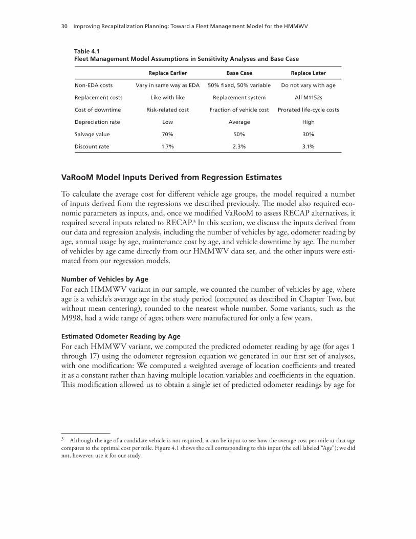
30 Improving Recapitalization Planning: Toward a Fleet Management Model for the HMMWV

Table 4.1Fleet Management Model Assumptions in Sensitivity Analyses and Base Case

Replace Earlier Base Case Replace Later

Non-EDA costs Vary in same way as EDA 50% fixed, 50% variable Do not vary with age

Replacement costs Like with like Replacement system All M1152s

Cost of downtime Risk-related cost Fraction of vehicle cost Prorated life-cycle costs

Depreciation rate Low Average High

Salvage value 70% 50% 30%

Discount rate 1.7% 2.3% 3.1%

VaRooM Model Inputs Derived from Regression Estimates

To calculate the average cost for different vehicle age groups, the model required a number of inputs derived from the regressions we described previously. The model also required eco-nomic parameters as inputs, and, once we modified VaRooM to assess RECAP alternatives, it required several inputs related to RECAP.3 In this section, we discuss the inputs derived from our data and regression analysis, including the number of vehicles by age, odometer reading by age, annual usage by age, maintenance cost by age, and vehicle downtime by age. The number of vehicles by age came directly from our HMMWV data set, and the other inputs were esti-mated from our regression models.

Number of Vehicles by Age

For each HMMWV variant in our sample, we counted the number of vehicles by age, where age is a vehicle’s average age in the study period (computed as described in Chapter Two, but without mean centering), rounded to the nearest whole number. Some variants, such as the M998, had a wide range of ages; others were manufactured for only a few years.

Estimated Odometer Reading by Age

For each HMMWV variant, we computed the predicted odometer reading by age (for ages 1 through 17) using the odometer regression equation we generated in our first set of analyses, with one modification: We computed a weighted average of location coefficients and treated it as a constant rather than having multiple location variables and coefficients in the equation. This modification allowed us to obtain a single set of predicted odometer readings by age for

3 Although the age of a candidate vehicle is not required, it can be input to see how the average cost per mile at that age compares to the optimal cost per mile. Figure 4.1 shows the cell corresponding to this input (the cell labeled “Age”); we did not, however, use it for our study.

Application of the Vehicle Replacement Model 31

each HMMWV variant rather than having a set for each combination of HMMWV variant and location.4

Annual Mileage by Age

We divided each predicted odometer reading by its corresponding age to get another input for the VaRooM model: annual mileage by age. The VaRooM model required an annual mile-age figure for each age in the range of possible HMMWV ages (1 through 17 years old). Each HMMWV variant typically had vehicles in a portion of that age range (e.g., ages 8 through 12) but not in the full range. Thus, to ensure that each variant had an annual mileage figure for the full set of ages 1 through 17, we computed approximate annual mileage by age from predicted odometer readings.

Estimated Annual Down Days by Age

Our downtime regression equations yielded predicted down days by age for each HMMWV variant.5 Once again, we computed a weighted average of location coefficients and treated that figure as a constant in the equation. The annual mileage-by-age figures (based on predicted odometer readings for each variant) served as usage values in the equations.

Estimated Annual Parts and Labor Cost by Age

We used our repair-cost regression equations to predict annual EDA-based parts and labor costs for each HMMWV variant. Again, we modified the equations so that they incorporated a weighted average of location coefficients as a constant rather than separate location variables and coefficients, and we treated the variant’s annual mileage-by-age figures as usage values in the equations.

After calculating EDA-based repair costs by age, we scaled them up to account for non-EDA costs. That is, because EDA data include only mission-critical failures with downtimes of at least one day, we needed to account for costs associated with other types of repairs. We devised two different methods for scaling up costs that can be thought of as establishing lower and upper bounds for actual cost variation by age. The first method assumed that non-EDA costs did not vary with vehicle age (a conservative assumption that sets a lower bound for cost variation with age) and estimated the difference between EDA repair costs per vehicle and non-EDA costs per vehicle. This method yielded a constant adjustment factor of $2,998.76. Under this “fixed-cost” assumption, one simply adds $2,998.76 to the annual EDA repair costs for

4 Had we not used a weighted average of location coefficients, we would have had separate predicted odometer read-ings by age for each HMMWV variant–location combination. We would then have needed 12 VaRooM worksheets (for 12 locations) for each of the 15 HMMWV variants. Since a VaRooM model with 180 worksheets would have been too unwieldy, we used the weighted average of location coefficients to yield one set of predictions—and one worksheet—for each HMMWV variant. These can be interpreted as one Army-wide average for each variant.5 In keeping with Army practice, we counted only downtime associated with NMC failures. Other private- and public-sector fleets also count downtime associated with scheduled services and with other unscheduled repairs, which results in higher costs of downtime and earlier optimal replacement ages.

32 Improving Recapitalization Planning: Toward a Fleet Management Model for the HMMWV

a HMMWV to account for non-EDA costs.6 We used this assumption for the replace-later case.

The second method for scaling up costs assumed that non-EDA costs vary in the same way EDA costs do with the age of the vehicle, which creates an upper bound for cost variation with age. For this method, one multiplies annual EDA costs by an adjustment factor of 4.78, based on a comparison of average EDA parts costs per vehicle and average OSMIS parts costs per vehicle.7 We used this assumption for the replace-earlier case.

For the base case, we used an intermediate assumption when scaling up our EDA repair-cost calculations in order to capture non-EDA costs. We assumed that 50 percent of those non-EDA costs were fixed costs and that 50 percent were variable. Thus, we calculated total repair costs as follows:

Total repair costs constant factor ED= +( . )0 5 ( AA repair costs

variable factor

)

+ ( . )(0 5 ))( )EDA repair costs

where the constant factor equaled $2,998.76, and the variable factor equaled 4.78.8

Economic Parameters

In addition to the regression-based inputs described previously, the VaRooM model required economic factors as inputs—more specifically, fixed and variable economic parameters that influence the life-cycle costs of a vehicle. Fixed parameter inputs included the opportunity cost incurred for each day of equipment downtime, the annual discount rate, and a salvage factor. A variable parameter input was the set of depreciation rates. This input was allowed to vary because depreciation rate can change with vehicle age. For example, the resale value of a vehicle typically falls more quickly in the first few years than it does in later years.

In this section, we define the parameters and discuss each set of assumptions that we made to examine the model’s sensitivity.

6 Between the first quarter of FY01 and the third quarter of FY02, the HMMWVs in our data set (covering locations in FORSCOM, TRADOC, USAREUR, and EUSA) had an average parts cost per vehicle of $161.82, in FY03 dollars, and an average quarterly parts-plus-labor cost per vehicle of $198.08. This suggests that labor costs were approximately 22.41 percent of parts costs. In OSMIS, the average quarterly parts cost per HMMWV at those locations during the same period was $774.26. Scaling up OSMIS costs by 22.41 percent yielded a quarterly figure of $947.77, and subtracting EDA parts and labor costs from that figure gave additional costs of $749.69. Annualizing this quarterly figure (multiplying it by four) resulted in a constant factor of $2,998.76.7 The average quarterly parts cost per vehicle for HMMWVs in our sample was $161.82; the average quarterly parts cost per vehicle in OSMIS for HMMWVs for the same locations and time period was $774.26. Dividing $774.26 by $161.82 yielded 4.78, our variable factor.8 These assumptions affect the intercept and the slope of the relationship between maintenance cost and age. A steeper slope (i.e., assuming that non-EDA costs vary in the same way that EDA costs do) will lead to an earlier optimal replace-ment age, whereas a flatter slope (i.e., assuming that non-EDA costs do not vary with age and adding them to the intercept) will lead to a later optimal replacement age.

Application of the Vehicle Replacement Model 33

Replacement Cost

Replacement cost refers to the acquisition price of the replacement vehicle. The cost we used depended on whether we assumed that a given HMMWV variant was replaced with the same variant or with a modernized version. All figures were based on Army Master Data File (AMDF) prices and were in FY03 dollars.

The base-case vehicle-replacement cost was the AMDF acquisition price of the planned-replacement system adjusted for inflation. For the replace-earlier case, we assumed that each vehicle would be replaced by a vehicle of the same variant (i.e., “like with like” replacement), so the vehicle replacement cost was the AMDF acquisition price of the original variant adjusted for inflation. For the replace-later case, we assumed that all variants would be replaced with the M1152 (costing $133,341 in FY03 dollars) except for the M1114, which would be replaced by another M1114 at a cost of $161,528.

Table 4.2 shows the original variant and its acquisition price, along with the planned-replacement variant (based on information provided by HQDA G-8) and its acquisition price.

Cost of Downtime

The cost of downtime is defined as the daily cost (dollars per vehicle per day) of being without a piece of equipment. Typically, when a piece or fleet of equipment incurs downtime, additional equipment needs to be on hand to cover the requirements. Fleet managers sometimes calcu-late the opportunity cost of downtime as the cost to rent replacement vehicles or equipment to fulfill a requirement.

Our base-case cost of downtime was the replacement cost divided by 365 days; this value was in the range of $100 to $400 per day, which is similar to the daily cost of renting a com-mercial Hummer9 and served as an imputed daily rental rate based on the vehicle’s replacement value.

For the replace-earlier case, we multiplied the base-case downtime cost by a risk factor of 3.0, which assumes that the cost goes up 200 percent if downtime prevents completion of a mission. The downtime cost for the replace-earlier case was thus the base-case replacement cost divided by 365, multiplied by 3.0.10 For the replace-later case, we assumed that the size of the HMMWV fleet was large enough that an out-of-service HMMWV was not critical to meeting mission requirements. We thus divided the AAOC at the variant’s modal age by 365 to get the daily cost of downtime for this case.11

9 Rental rates for Hummers in the United States as of December 2006 ranged from $150 to $400 per day depending on model and location. Daily rental rates for Hummers in Europe were in the range of $750 to $1,000. (Rental rates obtained from http://www.autoboutiquerental.com, http://www.bhrentacar.com, http://www.rentexoticcars.com, http://www.exoticcarrentalsphoenix.com, and http://www.eliterent.com on December 20, 2006.) The manufacturer’s suggested retail prices of Hummer models are approximately $128,000 for the H1, $53,000 for the H2, and $29,000 for the H3 (http://www.automotive.com/new-cars/pricing/01/hummer/index.html, as of December 20, 2006).10 Since it is difficult to monetize the potential cost associated with a vehicle being unavailable to complete a mission, we selected a risk factor to test the sensitivity of the model to an increased cost of downtime.11 For example, the modal age of the M998 was 13 years. The annualized replacement cost for a 13-year-old M998 was its acquisition price divided by one plus the vehicle’s age, or $39,251/(1+13) = $2,803.64. Repair costs for a 13-year-old

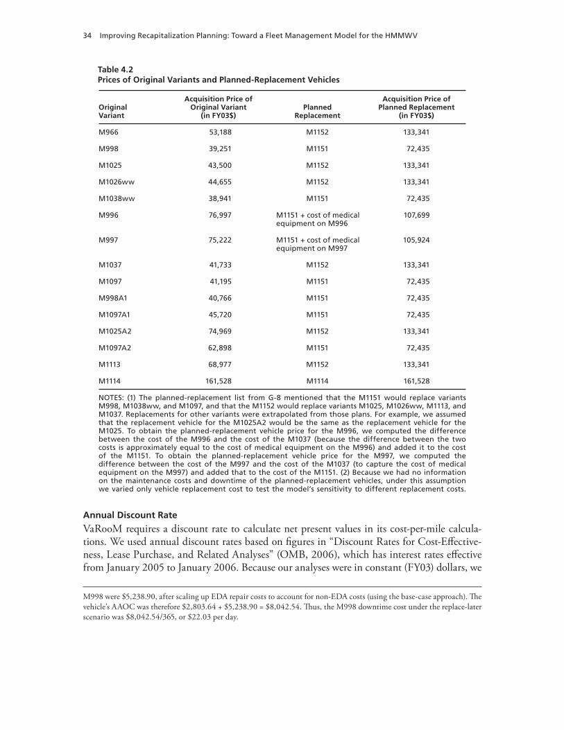
34 Improving Recapitalization Planning: Toward a Fleet Management Model for the HMMWV

Table 4.2Prices of Original Variants and Planned-Replacement Vehicles

Original Variant

Acquisition Price of Original Variant

(in FY03$)Planned

Replacement

Acquisition Price of Planned Replacement

(in FY03$)

M966 53,188 M1152 133,341

M998 39,251 M1151 72,435

M1025 43,500 M1152 133,341

M1026ww 44,655 M1152 133,341

M1038ww 38,941 M1151 72,435

M996 76,997 M1151 + cost of medical equipment on M996

107,699

M997 75,222 M1151 + cost of medical equipment on M997

105,924

M1037 41,733 M1152 133,341

M1097 41,195 M1151 72,435

M998A1 40,766 M1151 72,435

M1097A1 45,720 M1151 72,435

M1025A2 74,969 M1152 133,341

M1097A2 62,898 M1151 72,435

M1113 68,977 M1152 133,341

M1114 161,528 M1114 161,528

NOTES: (1) The planned-replacement list from G-8 mentioned that the M1151 would replace variants M998, M1038ww, and M1097, and that the M1152 would replace variants M1025, M1026ww, M1113, and M1037. Replacements for other variants were extrapolated from those plans. For example, we assumed that the replacement vehicle for the M1025A2 would be the same as the replacement vehicle for the M1025. To obtain the planned-replacement vehicle price for the M996, we computed the difference between the cost of the M996 and the cost of the M1037 (because the difference between the two costs is approximately equal to the cost of medical equipment on the M996) and added it to the cost of the M1151. To obtain the planned-replacement vehicle price for the M997, we computed the difference between the cost of the M997 and the cost of the M1037 (to capture the cost of medical equipment on the M997) and added that to the cost of the M1151. (2) Because we had no information on the maintenance costs and downtime of the planned-replacement vehicles, under this assumption we varied only vehicle replacement cost to test the model’s sensitivity to different replacement costs.

Annual Discount Rate

VaRooM requires a discount rate to calculate net present values in its cost-per-mile calcula-tions. We used annual discount rates based on figures in “Discount Rates for Cost-Effective-ness, Lease Purchase, and Related Analyses” (OMB, 2006), which has interest rates effective from January 2005 to January 2006. Because our analyses were in constant (FY03) dollars, we

M998 were $5,238.90, after scaling up EDA repair costs to account for non-EDA costs (using the base-case approach). The vehicle’s AAOC was therefore $2,803.64 + $5,238.90 = $8,042.54. Thus, the M998 downtime cost under the replace-later scenario was $8,042.54/365, or $22.03 per day.

Application of the Vehicle Replacement Model 35

used real interest rates.12 For the base case, we used a discount rate of 2.3 percent, the Treasury bond interest rate for a time horizon of seven years (roughly equivalent to the Program Objec-tive Memorandum period). For the replace-earlier case, the discount rate was 1.7 percent (3-year time horizon); for the replace-later case, it was 3.1 percent (30-year time horizon).

Depreciation Rates

Vehicles lose value over time due to wear and tear and to changes in technology. In the con-text of fleet management, the depreciation rate refers to the percentage by which the value of a vehicle decreases each year. VaRooM requires a set of depreciation rates as an input.13 Depre-ciation rates based on fair market values of HMMWVs are not available, because the Army does not sell used HMMWVs to the public. We consulted a variety of sources on residual values of comparable vehicles, such as passenger cars and trucks and construction equipment, and elected to use the car depreciation calculator from Money-Zine.com because it provided a range of “average,” “high,” and “low” depreciation rates that could be used to test the model’s sensitivity.14 Depreciation rates for various types of construction equipment showed similar patterns.

We used the following car depreciation rates: “average” rates for the base case, “low” rates for the replace-earlier case, and “high” rates for the replace-later case. Faster depreciation reduces the residual value of vehicles and tends to increase optimal replacement age.

Salvage Factor

The salvage factor, traditionally derived from historical data, refers to the average percentage of a vehicle’s depreciated value (acquisition price minus depreciation) that would be obtained upon retiring (e.g., selling) a typical vehicle.15 We assumed a salvage factor of 50 percent for the base case, 70 percent for the replace-earlier case, and 30 percent for the replace-later case. Since a lower salvage factor reduces the residual value of a vehicle, it tends to increase optimal replacement age.

Recapitalization Inputs

Our modified version of VaRooM calls for several inputs that were not in the original VaRooM model. These inputs, accompanied by additional Visual Basic code underlying the spreadsheet

12 OMB Circular A-94 (OMB, 1992, par. 8c(3)) states that when an investment has “internal” benefits, such as a reduction in government costs, it is appropriate to use a “comparable-maturity Treasury rate as a discount rate.” A higher discount rate tends to increase the optimal replacement age.13 In a private-sector context, depreciation affects the tax expenses or deductions associated with a vehicle. VaRooM can also calculate these effects as part of operating costs.14 See Lucko, 2003; Vorster, 2004, 2006; and money-zine.com (the car depreciation calculator we used is available at http://www.money-zine.com/Calculators/Auto-Loan-Calculators/Car-Depreciation-Calculator/).15 Since the Army does not sell used HMMWVs to the public, we examined the sales prices of military surplus trucks and truck tractors in April through May 2005 to check the reasonableness of the salvage values we used in the model. (Auction values obtained from http://www.govliquidation.com/list/c7587/cta/1.html on April 27, May 12, and May 25, 2005.)

36 Improving Recapitalization Planning: Toward a Fleet Management Model for the HMMWV

model, allow the model to assess RECAP alternatives. Rather than attempting to model the Army’s RECAP program for HMMWVs, which includes both the rebuilding and upgrad-ing of certain components, we modeled a simpler, hypothetical RECAP program based on a vehicle’s age at the time of RECAP, the cost of RECAP for that vehicle, and the effective age to which RECAP returns that vehicle. We then examined those combinations of values for these three parameters for which a RECAP program would be cost-effective. A RECAP pro-gram that results in higher capabilities than those of the original vehicles cannot be evaluated solely on cost.

Year of Recapitalization

The year of RECAP refers to the vehicle age at which a planned rebuild or upgrade could occur. We varied this input to evaluate outcomes associated with alternative RECAP plans.

Recapitalization Cost

The RECAP cost refers to the planned expenditure, in dollars per vehicle, for rebuild or upgrade. We used notional values of $20,000, $25,000, and $30,000 per vehicle in this analysis. We also assumed that the vehicle was down for an additional 35 days in the year of RECAP, basing our assumption on the time needed to RECAP a HMMWV under the Army’s HMMWV RECAP program.16

Post-Recapitalization Age

A third input required for assessment of RECAP alternatives is the post-RECAP age, which we define as the effective age to which RECAP returns a vehicle. For example, if one plans to spend $20,000 to RECAP a vehicle at age 9, and if that rebuild or upgrade will make the vehicle behave like a 1-year-old vehicle in terms of maintenance requirements, then the year of RECAP is 9, RECAP cost is $20,000, and post-RECAP age is 1. The post-RECAP age cannot be greater than the RECAP year.

Our RECAP analyses assumed that when a vehicle is recapitalized, its repair costs, depre-ciation, and downtime return to the levels they had at the post-RECAP age and then grow over time, again based on our regression equations. For example, in Figure 4.1 (shown earlier), the year of RECAP is 9, and the post-RECAP age is 1. At age 9, the vehicle’s repair costs are therefore assumed to return to what they were at age 1. That is, at age 9, the cost-per-mile cal-culations begin to incorporate the maintenance costs in the column called “RECAP Maint Costs” rather than those in the column called “Smoothed Maint Cost.” If 9-year-old vehicles are returned to age 1, maintenance costs in the next year are assumed to be equivalent to those of a 2-year-old vehicle, even though the vehicles are 10 years old based on manufacture date. In the second year after RECAP, 11-year-old vehicles have maintenance costs equivalent to age 3, and so on.

We calculated post-RECAP salvage values by applying the post-RECAP depreciation rates to a revised valuation of the vehicle; this revised valuation consists of the cost of RECAP

16 Letterkenny Army Depot reported a HMMWV RECAP time (induction to paint) of approximately 34 days per vehicle as of April 2006 (Henke, 2006).

Application of the Vehicle Replacement Model 37

plus the vehicle’s depreciated value in the year of RECAP. For example, when the year of RECAP is 9 and the original replacement cost of the vehicle is $72,435, the depreciated value at age 9 (applying the depreciation rates in Figure 4.1) is $15,198. If the cost of RECAP is $20,000, the revised vehicle valuation equals $20,000 plus $15,198, or $35,198. We then apply the post-RECAP depreciation rates and the salvage factor to the figure of $35,198 to obtain post-RECAP salvage values.

Running the Model

When running the model for each HMMWV variant, we began by inserting the number of vehicles by age in the “Number of Vehicles” column of the spreadsheet, predicted odom-eter readings by age in the “Avg Cum Mileage” column, scaled-up repair costs by age in the “Parts & Labor Costs/Base Case” column, and predicted downtime by age in the “Downtime” column. Next, to determine a variant’s optimal replacement age without RECAP, we inserted its replacement cost (acquisition price shown in Table 4.1) in the “Replacement Cost” cell of the spreadsheet, and we inserted zeros in the cells called “Year of RECAP,” “RECAP Cost,” and “Post-RECAP Age.” The model’s key outputs—optimal replacement age and average cost per mile associated with that replacement age—then appeared in the “Optimal Replacement Age” and “Optimal Cost” cells, respectively.

To determine a variant’s optimal replacement age with RECAP, we had to evaluate a vari-ety of cases with different values for RECAP cost, year of RECAP, and post-RECAP age. For a given cost of RECAP and post-RECAP age, we identified the optimal year of RECAP by comparing the cases and selecting the year of RECAP with the lowest cost per mile.17 In these cases, rather than inserting zeros in the “Year of RECAP,” “RECAP Cost,” and “Post-RECAP Age” cells, we inserted, respectively, an age of vehicle RECAP, a total RECAP expenditure, and a post-RECAP age. For the M998, we tested alternative combinations of RECAP year and post-RECAP age, varying the RECAP year from 5 to 17 and, for each RECAP year, varying the post-RECAP age from 0 to the RECAP year.

Next, we eliminated those RECAP alternatives (combinations of RECAP year and post-RECAP age) that fared worse than did the alternative of no RECAP at all. The key crite-ria were the variant’s optimal cost per mile and the replacement age without RECAP. For example, without RECAP, the M998 had an optimal cost per mile of $5.53 associated with a replacement age of 12. We therefore rejected those RECAP alternatives that either (a) yielded an optimal cost per mile greater than $5.53 or (b) yielded an optimal cost per mile equal to $5.53 but an optimal replacement age less than or equal to 12. This left us with a smaller, pre-liminary set of potential RECAP alternatives with a positive return (e.g., RECAP year of 9, post-RECAP age of 1).

One can choose an alternative from the feasible set based on the expected post-RECAP age associated with one’s RECAP expenditure. For example, if one expects an expenditure (i.e.,

17 Only the year of RECAP can be optimized in this sense, because lower RECAP costs and lower post-RECAP ages are always preferred to higher ones.

38 Improving Recapitalization Planning: Toward a Fleet Management Model for the HMMWV

RECAP cost) of $20,000 to return a vehicle to age 1, then one can look within the feasible set of alternatives and choose the year of RECAP that yields the minimum average cost per mile given a post-RECAP age of 1.

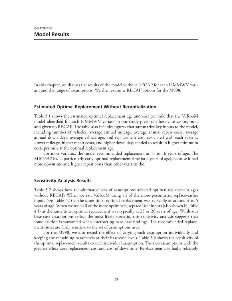
39

CHAPTER FIVE

Model Results

In this chapter, we discuss the results of the model without RECAP for each HMMWV vari-ant and the range of assumptions. We then examine RECAP options for the M998.

Estimated Optimal Replacement Without Recapitalization

Table 5.1 shows the estimated optimal replacement age and cost per mile that the VaRooM model identified for each HMMWV variant in our study given our base-case assumptions and given no RECAP. The table also includes figures that summarize key inputs to the model, including number of vehicles, average annual mileage, average annual repair costs, average annual down days, average vehicle age, and replacement cost associated with each variant. Lower mileage, higher repair costs, and higher down days tended to result in higher minimum costs per mile at the optimal replacement age.

For most variants, the model recommended replacement at 11 to 16 years of age. The M1025A2 had a particularly early optimal replacement time (at 9 years of age), because it had more downtime and higher repair costs than other variants did.

Sensitivity Analysis Results

Table 5.2 shows how the alternative sets of assumptions affected optimal replacement ages without RECAP. When we ran VaRooM using all of the more pessimistic, replace-earlier inputs (see Table 4.1) at the same time, optimal replacement was typically at around 4 to 5 years of age. When we used all of the more optimistic, replace-later inputs (also shown in Table 4.1) at the same time, optimal replacement was typically at 25 or 26 years of age. While our base-case assumptions reflect the most likely scenario, this sensitivity analysis suggests that some caution is warranted when interpreting base-case findings: The recommended replace-ment times are fairly sensitive to the set of assumptions used.

For the M998, we also tested the effect of varying each assumption individually and keeping the remaining parameters at their base-case levels. Table 5.3 shows the sensitivity of the optimal replacement results to each individual assumption. The two assumptions with the greatest effect were replacement cost and cost of downtime. Replacement cost had a relatively

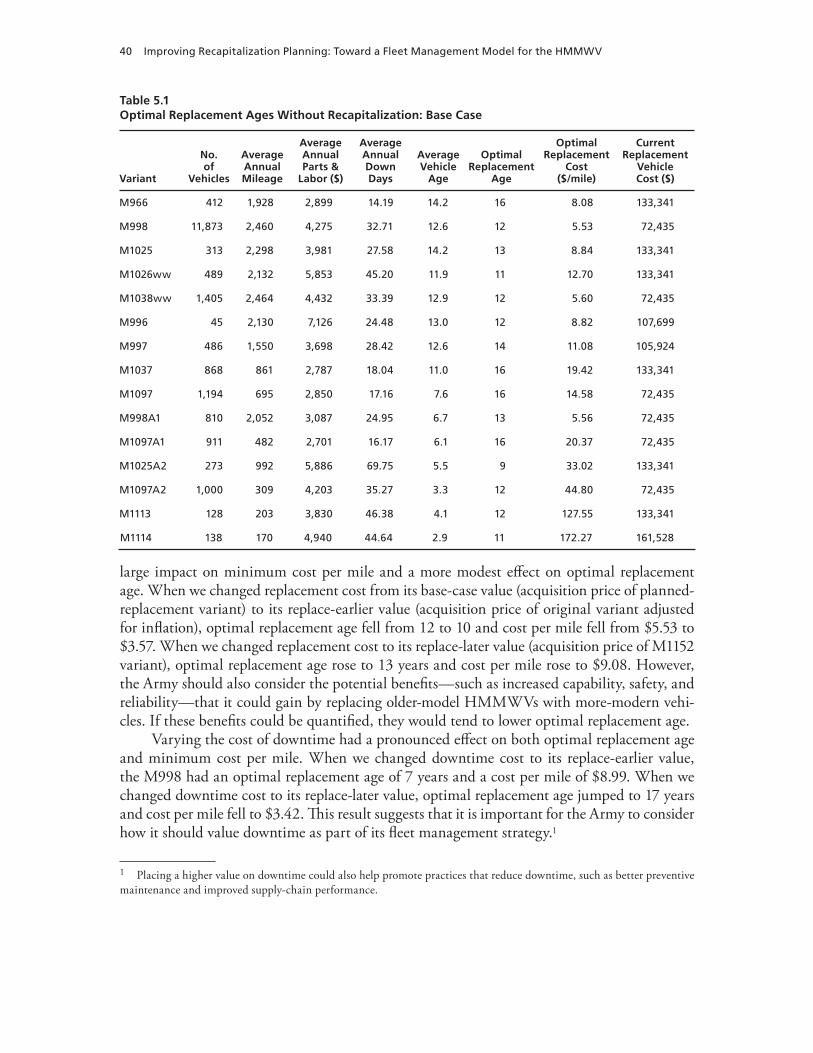
40 Improving Recapitalization Planning: Toward a Fleet Management Model for the HMMWV

Table 5.1 Optimal Replacement Ages Without Recapitalization: Base Case

Variant

No. of

Vehicles

Average Annual Mileage

Average Annual Parts &

Labor ($)

Average Annual Down Days

Average Vehicle

Age

Optimal Replacement

Age

Optimal Replacement

Cost ($/mile)

Current Replacement

Vehicle Cost ($)

M966 412 1,928 2,899 14.19 14.2 16 8.08 133,341

M998 11,873 2,460 4,275 32.71 12.6 12 5.53 72,435

M1025 313 2,298 3,981 27.58 14.2 13 8.84 133,341

M1026ww 489 2,132 5,853 45.20 11.9 11 12.70 133,341

M1038ww 1,405 2,464 4,432 33.39 12.9 12 5.60 72,435

M996 45 2,130 7,126 24.48 13.0 12 8.82 107,699

M997 486 1,550 3,698 28.42 12.6 14 11.08 105,924

M1037 868 861 2,787 18.04 11.0 16 19.42 133,341

M1097 1,194 695 2,850 17.16 7.6 16 14.58 72,435

M998A1 810 2,052 3,087 24.95 6.7 13 5.56 72,435

M1097A1 911 482 2,701 16.17 6.1 16 20.37 72,435

M1025A2 273 992 5,886 69.75 5.5 9 33.02 133,341

M1097A2 1,000 309 4,203 35.27 3.3 12 44.80 72,435

M1113 128 203 3,830 46.38 4.1 12 127.55 133,341

M1114 138 170 4,940 44.64 2.9 11 172.27 161,528

large impact on minimum cost per mile and a more modest effect on optimal replacement age. When we changed replacement cost from its base-case value (acquisition price of planned-replacement variant) to its replace-earlier value (acquisition price of original variant adjusted for inflation), optimal replacement age fell from 12 to 10 and cost per mile fell from $5.53 to $3.57. When we changed replacement cost to its replace-later value (acquisition price of M1152 variant), optimal replacement age rose to 13 years and cost per mile rose to $9.08. However, the Army should also consider the potential benefits—such as increased capability, safety, and reliability—that it could gain by replacing older-model HMMWVs with more-modern vehi-cles. If these benefits could be quantified, they would tend to lower optimal replacement age.

Varying the cost of downtime had a pronounced effect on both optimal replacement age and minimum cost per mile. When we changed downtime cost to its replace-earlier value, the M998 had an optimal replacement age of 7 years and a cost per mile of $8.99. When we changed downtime cost to its replace-later value, optimal replacement age jumped to 17 years and cost per mile fell to $3.42. This result suggests that it is important for the Army to consider how it should value downtime as part of its fleet management strategy.1

1 Placing a higher value on downtime could also help promote practices that reduce downtime, such as better preventive maintenance and improved supply-chain performance.

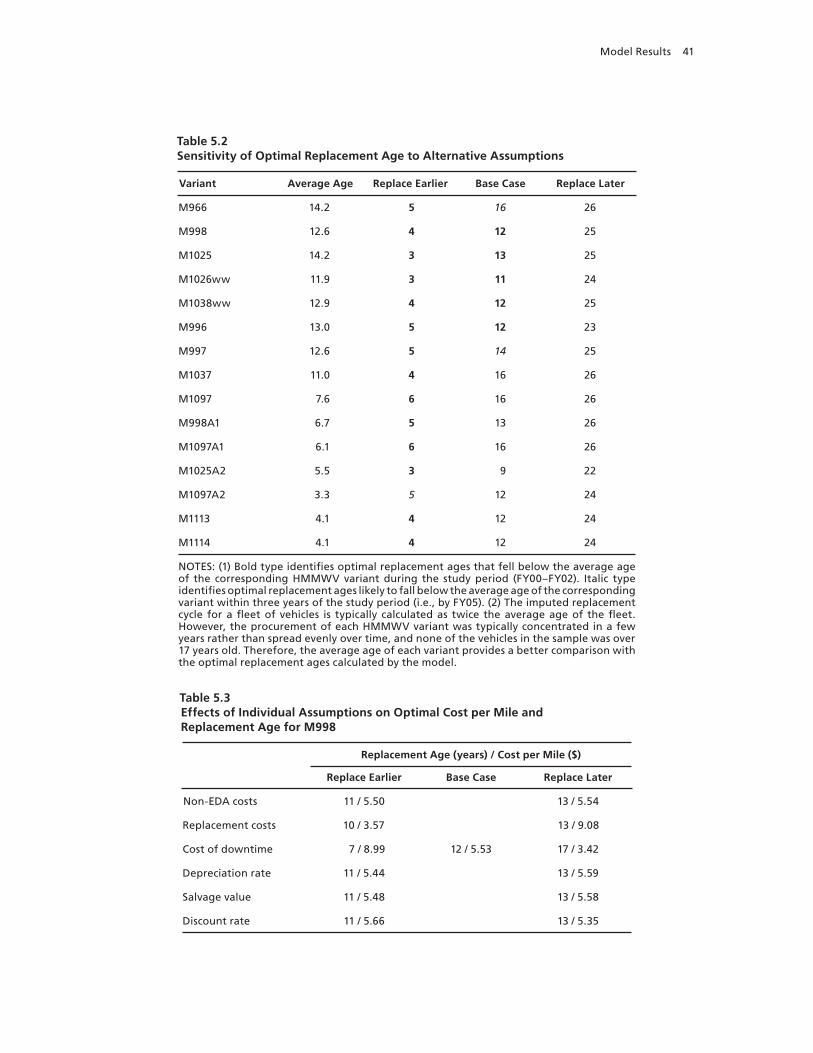
Model Results 41

Table 5.2 Sensitivity of Optimal Replacement Age to Alternative Assumptions

Variant Average Age Replace Earlier Base Case Replace Later

M966 14.2 5 16 26

M998 12.6 4 12 25

M1025 14.2 3 13 25

M1026ww 11.9 3 11 24

M1038ww 12.9 4 12 25

M996 13.0 5 12 23

M997 12.6 5 14 25

M1037 11.0 4 16 26

M1097 7.6 6 16 26

M998A1 6.7 5 13 26

M1097A1 6.1 6 16 26

M1025A2 5.5 3 9 22

M1097A2 3.3 5 12 24

M1113 4.1 4 12 24

M1114 4.1 4 12 24

NOTES: (1) Bold type identifies optimal replacement ages that fell below the average age of the corresponding HMMWV variant during the study period (FY00–FY02). Italic type identifies optimal replacement ages likely to fall below the average age of the corresponding variant within three years of the study period (i.e., by FY05). (2) The imputed replacement cycle for a fleet of vehicles is typically calculated as twice the average age of the fleet. However, the procurement of each HMMWV variant was typically concentrated in a few years rather than spread evenly over time, and none of the vehicles in the sample was over 17 years old. Therefore, the average age of each variant provides a better comparison with the optimal replacement ages calculated by the model.

Table 5.3Effects of Individual Assumptions on Optimal Cost per Mile and Replacement Age for M998

Replacement Age (years) / Cost per Mile ($)

Replace Earlier Base Case Replace Later

Non-EDA costs 11 / 5.50 13 / 5.54

Replacement costs 10 / 3.57 13 / 9.08

Cost of downtime 7 / 8.99 12 / 5.53 17 / 3.42

Depreciation rate 11 / 5.44 13 / 5.59

Salvage value 11 / 5.48 13 / 5.58

Discount rate 11 / 5.66 13 / 5.35

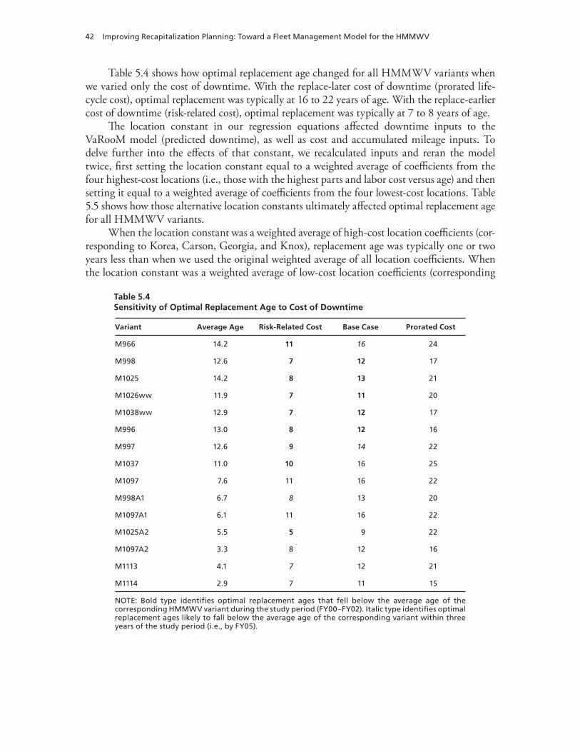
42 Improving Recapitalization Planning: Toward a Fleet Management Model for the HMMWV

Table 5.4 shows how optimal replacement age changed for all HMMWV variants when we varied only the cost of downtime. With the replace-later cost of downtime (prorated life-cycle cost), optimal replacement was typically at 16 to 22 years of age. With the replace-earlier cost of downtime (risk-related cost), optimal replacement was typically at 7 to 8 years of age.

The location constant in our regression equations affected downtime inputs to the VaRooM model (predicted downtime), as well as cost and accumulated mileage inputs. To delve further into the effects of that constant, we recalculated inputs and reran the model twice, first setting the location constant equal to a weighted average of coefficients from the four highest-cost locations (i.e., those with the highest parts and labor cost versus age) and then setting it equal to a weighted average of coefficients from the four lowest-cost locations. Table 5.5 shows how those alternative location constants ultimately affected optimal replacement age for all HMMWV variants.

When the location constant was a weighted average of high-cost location coefficients (cor-responding to Korea, Carson, Georgia, and Knox), replacement age was typically one or two years less than when we used the original weighted average of all location coefficients. When the location constant was a weighted average of low-cost location coefficients (corresponding

Table 5.4Sensitivity of Optimal Replacement Age to Cost of Downtime

Variant Average Age Risk-Related Cost Base Case Prorated Cost

M966 14.2 11 16 24

M998 12.6 7 12 17

M1025 14.2 8 13 21

M1026ww 11.9 7 11 20

M1038ww 12.9 7 12 17

M996 13.0 8 12 16

M997 12.6 9 14 22

M1037 11.0 10 16 25

M1097 7.6 11 16 22

M998A1 6.7 8 13 20

M1097A1 6.1 11 16 22

M1025A2 5.5 5 9 22

M1097A2 3.3 8 12 16

M1113 4.1 7 12 21

M1114 2.9 7 11 15

NOTE: Bold type identifies optimal replacement ages that fell below the average age of the corresponding HMMWV variant during the study period (FY00–FY02). Italic type identifies optimal replacement ages likely to fall below the average age of the corresponding variant within three years of the study period (i.e., by FY05).

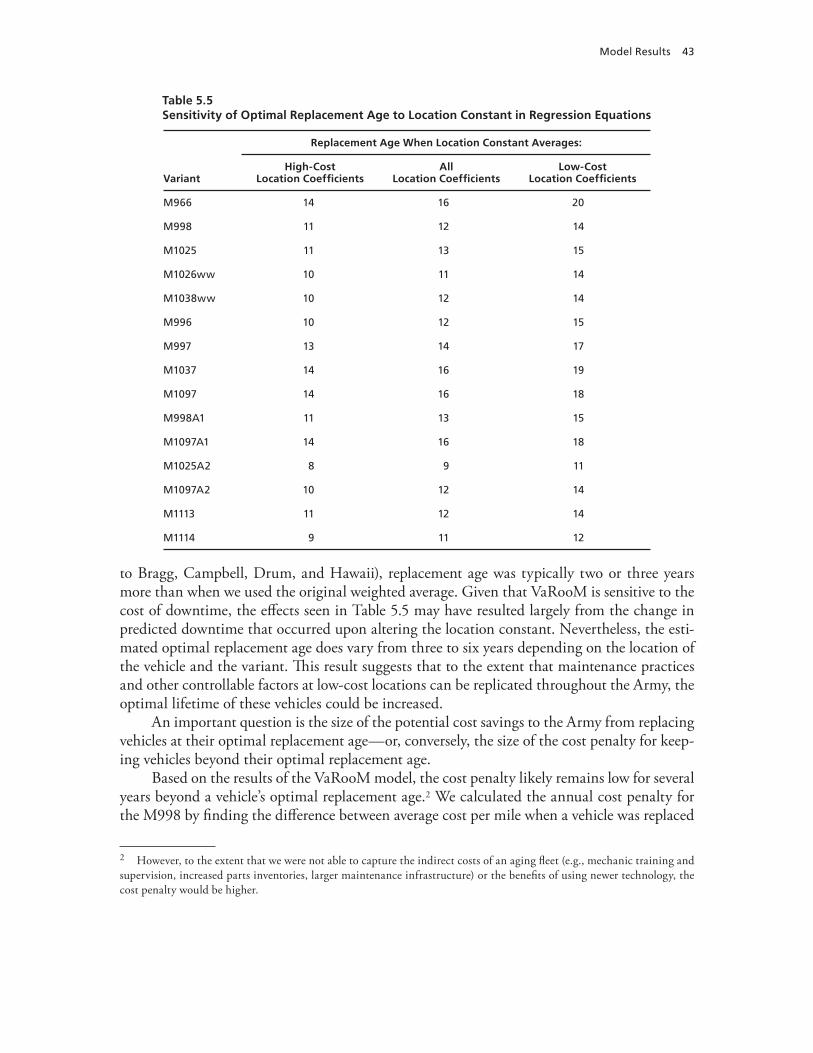
Model Results 43

Table 5.5Sensitivity of Optimal Replacement Age to Location Constant in Regression Equations

Variant

Replacement Age When Location Constant Averages:

High-Cost Location Coefficients

All Location Coefficients

Low-Cost Location Coefficients

M966 14 16 20

M998 11 12 14

M1025 11 13 15

M1026ww 10 11 14

M1038ww 10 12 14

M996 10 12 15

M997 13 14 17

M1037 14 16 19

M1097 14 16 18

M998A1 11 13 15

M1097A1 14 16 18

M1025A2 8 9 11

M1097A2 10 12 14

M1113 11 12 14

M1114 9 11 12

to Bragg, Campbell, Drum, and Hawaii), replacement age was typically two or three years more than when we used the original weighted average. Given that VaRooM is sensitive to the cost of downtime, the effects seen in Table 5.5 may have resulted largely from the change in predicted downtime that occurred upon altering the location constant. Nevertheless, the esti-mated optimal replacement age does vary from three to six years depending on the location of the vehicle and the variant. This result suggests that to the extent that maintenance practices and other controllable factors at low-cost locations can be replicated throughout the Army, the optimal lifetime of these vehicles could be increased.

An important question is the size of the potential cost savings to the Army from replacing vehicles at their optimal replacement age—or, conversely, the size of the cost penalty for keep-ing vehicles beyond their optimal replacement age.

Based on the results of the VaRooM model, the cost penalty likely remains low for several years beyond a vehicle’s optimal replacement age.2 We calculated the annual cost penalty for the M998 by finding the difference between average cost per mile when a vehicle was replaced

2 However, to the extent that we were not able to capture the indirect costs of an aging fleet (e.g., mechanic training and supervision, increased parts inventories, larger maintenance infrastructure) or the benefits of using newer technology, the cost penalty would be higher.

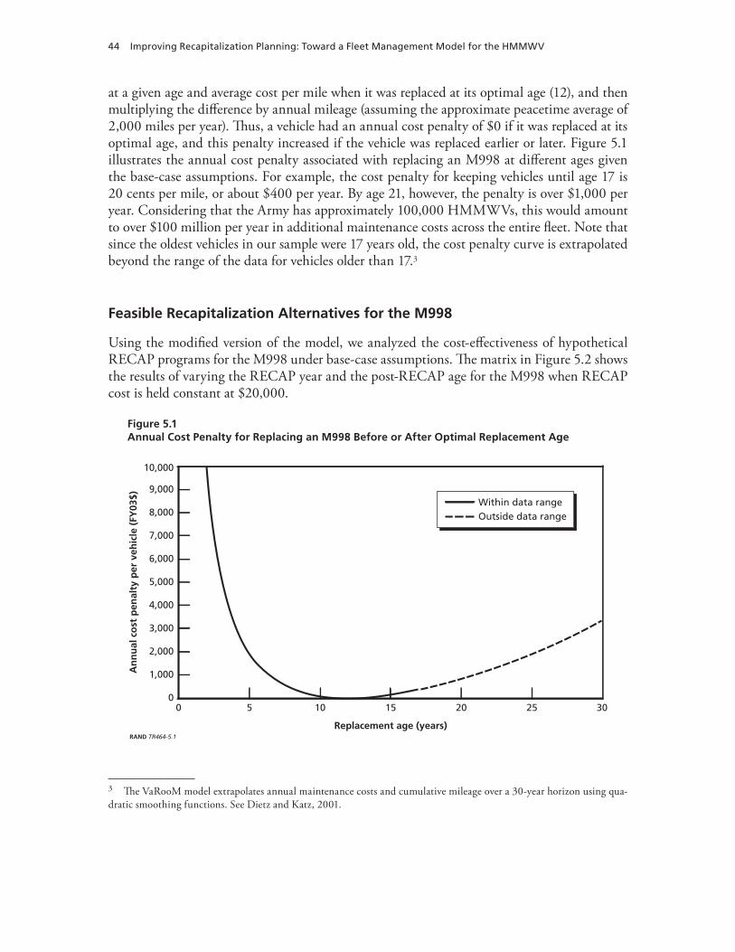
44 Improving Recapitalization Planning: Toward a Fleet Management Model for the HMMWV

at a given age and average cost per mile when it was replaced at its optimal age (12), and then multiplying the difference by annual mileage (assuming the approximate peacetime average of 2,000 miles per year). Thus, a vehicle had an annual cost penalty of $0 if it was replaced at its optimal age, and this penalty increased if the vehicle was replaced earlier or later. Figure 5.1 illustrates the annual cost penalty associated with replacing an M998 at different ages given the base-case assumptions. For example, the cost penalty for keeping vehicles until age 17 is 20 cents per mile, or about $400 per year. By age 21, however, the penalty is over $1,000 per year. Considering that the Army has approximately 100,000 HMMWVs, this would amount to over $100 million per year in additional maintenance costs across the entire fleet. Note that since the oldest vehicles in our sample were 17 years old, the cost penalty curve is extrapolated beyond the range of the data for vehicles older than 17.3

Feasible Recapitalization Alternatives for the M998

Using the modified version of the model, we analyzed the cost-effectiveness of hypothetical RECAP programs for the M998 under base-case assumptions. The matrix in Figure 5.2 shows the results of varying the RECAP year and the post-RECAP age for the M998 when RECAP cost is held constant at $20,000.

Figure 5.1Annual Cost Penalty for Replacing an M998 Before or After Optimal Replacement Age

9,000

8,000

7,000

6,000

5,000

4,000

3,000

2,000

1,000

10,000

302520151050

Replacement age (years)

An

nu

al c

ost

pen

alty

per

veh

icle

(FY

03$)

0

RAND TR464-5.1

Within data rangeOutside data range

3 The VaRooM model extrapolates annual maintenance costs and cumulative mileage over a 30-year horizon using qua-dratic smoothing functions. See Dietz and Katz, 2001.

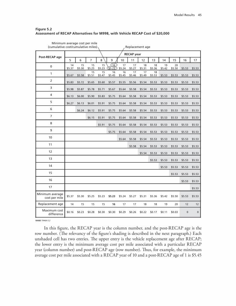
Model Results 45

Figure 5.2Assessment of RECAP Alternatives for M998, with Vehicle RECAP Cost of $20,000

1615141312111098765 17

Replacement ageMinimum average cost per mile

(cumulative cost/cumulative miles)

Post-RECAP ageRECAP year

0

1

2

3

4

5

6

7

8

9

10

11

12

13

14

15

16

17

Minimum averagecost per mile

Replacement age

Maximum costdifference

RAND TR464-5.2

14$5.37

$5.67

$5.83

$5.98

$6.13

$6.27

15$5.30

$5.58

$5.72

$5.87

$6.00

$6.13

$6.24

15$5.25

15$5.51

$5.65

$5.78

$5.90

$6.01

$6.12

$6.15

15$5.23

15$5.47

$5.60

$5.71

$5.83

$5.91

$5.91

$5.91

$5.91

16$5.23

16$5.45

$5.57

$5.67

$5.75

$5.75

$5.75

$5.75

$5.75

$5.75

17$5.24

16$5.45

$5.55

$5.64

$5.64

$5.64

$5.64

$5.64

$5.64

$5.64

$5.64

17$5.27

17$5.46

$5.56

$5.58

$5.58

$5.58

$5.58

$5.58

$5.58

$5.58

$5.58

$5.58

18$5.31

17$5.49

$5.54

$5.54

$5.54

$5.54

$5.54

$5.54

$5.54

$5.54

$5.54

$5.54

$5.54

18$5.36

18$5.53

$5.53

$5.53

$5.53

$5.53

$5.53

$5.53

$5.53

$5.53

$5.53

$5.53

$5.53

$5.53

19$5.42

$5.53

$5.53

$5.53

$5.53

$5.53

$5.53

$5.53

$5.53

$5.53

$5.53

$5.53

$5.53

$5.53

$5.53

20$5.50

$5.53

$5.53

$5.53

$5.53

$5.53

$5.53

$5.53

$5.53

$5.53

$5.53

$5.53

$5.53

$5.53

$5.53

$5.53

$5.53

$5.53

$5.53

$5.53

$5.53

$5.53

$5.53

$5.53

$5.53

$5.53

$5.53

$5.53

$5.53

$5.53

$5.53

$5.53

$5.53

$5.53

$5.53

$5.53

$5.53

$5.53

$5.53

$5.53

$5.53

$5.53

$5.53

$5.53

$5.53

$5.53

$5.53

$5.53

$5.53

$5.53

$5.53

$5.37

14

$0.16

$5.30

15

$0.23

$5.25

15

$0.28

$5.23

15

$0.30

$5.23

16

$0.30

$5.24

17

$0.29

$5.27

17

$0.26

$5.31

18

$0.22

$5.36

18

$0.17

$5.42

19

$0.11

$5.50

20

$0.03

$5.53

12

0

$5.53

12

0

In this figure, the RECAP year is the column number, and the post-RECAP age is the row number. (The relevancy of the figure’s shading is described in the next paragraph.) Each unshaded cell has two entries. The upper entry is the vehicle replacement age after RECAP; the lower entry is the minimum average cost per mile associated with a particular RECAP year (column number) and post-RECAP age (row number). Thus, for example, the minimum average cost per mile associated with a RECAP year of 10 and a post-RECAP age of 1 is $5.45

46 Improving Recapitalization Planning: Toward a Fleet Management Model for the HMMWV

with vehicle replacement at age 16. This means that if one plans to recapitalize an M998 when it is 10 years old and expects this RECAP to bring the vehicle back to age 1, then one should replace the vehicle at age 16. In other words, replacement at age 16 will result in the minimum average cost per mile under the stated conditions.

We determined the cost-effectiveness of alternatives by comparing their minimum aver-age costs per mile, and then their replacement ages, to those of the no-RECAP alternative (optimal replacement without RECAP). Each shaded cell in Figure 5.2 represents an alterna-tive that is not cost-effective—i.e., a RECAP alternative for which the minimum average cost per mile was (a) greater than that of the no-RECAP alternative ($5.53) or (b) equal to that of the no-RECAP alternative but with a replacement age less than or equal to that of the no-RECAP alternative (age 12). If a RECAP alternative yielded an average cost per mile of $5.53 but a replacement age greater than 12, it was considered cost-effective.

Looking across each row, one sees an optimal RECAP year—i.e., a year that minimizes the cost per mile for a given post-RECAP age and RECAP cost. For example, for a post-RECAP age of 0, the optimal RECAP year is age 9, which results in a cost per mile of $5.23 and a replacement age of 16 (this solution is pointed out in the top row of Figure 5.2). As was the case with replacement, however, the cost penalty for delaying RECAP by a few years is not very large. If RECAP is delayed to age 11 in our example, the resulting minimum cost per mile is $5.27.

The set of feasible solutions4 for a RECAP cost of $20,000 per vehicle consists of the 18 white cells in Figure 5.2 that have post-RECAP ages ranging from 0 to 1. Table 5.6 shows how the number of feasible solutions decreased when we increased the RECAP cost from $20,000 to $30,000 per vehicle. An investment of $20,000 per vehicle yielded 18 feasible solutions. Even if RECAP were unable to return the vehicles to “like-new” condition (i.e., a post-RECAP age of 0), the $20,000 investment could still offer an average cost per mile better than that offered by the no-RECAP alternative.

In contrast, the $30,000 investment per vehicle yielded eight feasible solutions, each with a post-RECAP age of 0. This suggests that a $30,000 M998 RECAP can be justified on the

Table 5.6Effect of Alternative RECAP Expenditures on Set of Feasible Solutions

RECAP Cost($)

Number of Feasible Alternative

(of those tested)

Maximum Cost-Effective

Post-RECAP Age

Best Solution (Post-RECAP Age = 0)

RECAP Year Cost/Mile ($) Replacement Age

20,000 18 1 9 5.23 16

25,000 10 0 10 5.33 17

30,000 8 0 10 5.43 17

≥36,000 None None N/A 5.53 12

4 We define a solution as feasible if it reduces the life-cycle average cost per mile or extends the life of the vehicle when the life-cycle average cost per mile is held constant.

Model Results 47

basis of cost per mile only if that RECAP returns a vehicle to “like-new” condition (a post-RECAP age of 0).

As RECAP cost increases, the potential cost savings decline, as shown in Table 5.6. When RECAP costs $30,000, for instance, the lowest attainable cost per mile is $5.43. Note, however, that there may be justifications other than cost per mile for a particular investment. For example, a $30,000 RECAP that adds a new, much-needed capability may be warranted even if it does not yield a post-RECAP age of 0 or a cost per mile lower than $5.53. At a cost of $36,000 or higher, a RECAP is not cost-effective unless it offers capability beyond that of the original vehicle (upgrade rather than rebuild).

49

CHAPTER SIX

Implications

The objective of this study was to provide vehicle-level data and analyses, along with a deci-sion-support tool, to facilitate RECAP planning. Data sources such as LIDB and EDA (both currently accessible via LOGSA’s Logistics Information Warehouse) now permit studies incor-porating several years of age, usage, location, and mission-critical-failure data from individual vehicles. We used such data to quantify age, usage, and location effects on the repair costs and availability of HMMWVs. We then embedded the results of our analyses in a spreadsheet-based vehicle replacement model. This concluding chapter discusses the major implications of our research.

The first part of our study found that aging had significant effects on the cost and avail-ability of HMMWVs. When we looked at the M998 in particular, the predicted annual NMC repair costs for 17-year-old vehicles were typically five to six times higher than those for new vehicles. The second part of our study entailed adjusting for non-EDA costs using aggregate OSMIS data, which yielded a range of possible costs for older vehicles that depended on our assumption about how non-EDA costs varied. Ideally, this type of analysis should be based on vehicle-level data for all repair costs, a type of data that should be collected by the Army but currently is not.

We also found aging to have significant effects on HMMWV availability. Predicted downtime was about two to three times higher for a 17-year-old M998 than for a new vehi-cle—typically around 35 and 15 days per year for, respectively, the older vehicle and the new vehicle. Although these figures are within the Army’s 90 percent fleet availability goal, they are very high compared with figures for comparable public- and private-sector fleets.1 Like repair costs, these downtime figures may turn out to be higher during deployment, particularly since our regressions also revealed usage effects on costs and downtime.

Location effects were also noteworthy, as some sites (particularly Korea) had higher costs and downtime than did other sites (such as Fort Bragg). This pattern may reflect different terrains, climates, maintenance schedules, training-schedule profiles, and personnel skill sets across locations. To the extent that maintenance practices and other controllable factors at low-cost locations could be replicated throughout the Army, optimal vehicle lifetimes could be increased.

1 Other RAND Arroyo Center research (Held and Wolff, 2004) suggests that improved preventive maintenance pro-grams could improve reliability and reduce total maintenance costs.

50 Improving Recapitalization Planning: Toward a Fleet Management Model for the HMMWV

The explanatory power of our models was consistent with that of other studies involving two-part regressions. As Diehr et al. (1999, p. 134) noted in their analysis of health care utili-zation and costs:

In regression analyses of utilization data, the values of R2 are usually on the order of ≤20% [Newhouse, 1982]. This should not be surprising considering how difficult it would be to predict one’s own utilization. The low values of R2 indicate that we can not predict well for an individual; however, more often we are trying to predict the average cost for a group of individuals, and regression equations can often do this quite satisfactorily.

In our study, regression models explained only a small part of the variation at the individual vehicle level; however, they explained a larger part of the variation with respect to age groups, location groups, and usage groups. While actual repair costs for individual vehicles often varied widely from predicted costs, average repair costs by age were relatively close to the predictions. Similarly, the correlation between predicted and observed costs at the brigade and battalion levels of analysis was quite strong. In short, like health care utilization models, our models appear to be reasonable for predicting aggregate or average repair costs but not for predicting repair costs for a particular vehicle.2

In the second part of our study, we were able to identify specific vehicle replacement and RECAP recommendations based on our estimated cost-versus-age and downtime-versus-age relationships using the VaRooM vehicle replacement model. However, it is important to note that lack of clarity and consensus on some of the assumptions results in uncertainty around the optimal ages, and that small delays beyond the estimated optimal ages result in only small cost increases, further suggesting some uncertainty as to the optimal replacement and RECAP ages. Regardless, given a set of assumptions, this methodology should result in the lowest total ownership costs and likely provides better estimated optimal replacement and RECAP ages than can be provided by judgment alone.

Because age and usage had significant effects on vehicle costs and downtime, we were able to derive a set of predicted down days and predicted costs (scaled up to include non-EDA costs as well as EDA costs) for ages 0 to 17 for all 15 HMMWV variants in our sample. Those predictions served as inputs to the VaRooM model, and VaRooM, in turn, revealed the opti-mal replacement age for each variant. This feature of our study distinguishes it from previous studies that typically provided either statistical analyses or vehicle replacement models without integrating the two.

Replacement Without Recapitalization

Without RECAP, the HMMWV optimal replacement age ranged from 11 to 16 depending on the variant, with most variants having an estimated optimal replacement age of about 12.

2 However, note that greater variability in the repair costs of individual vehicles could increase indirect maintenance costs, such as mechanic training, supervision, parts inventories, and infrastructure. Increased preventive maintenance could reduce the variability of unscheduled repair costs, including costs associated with mission-critical failures.

Implications 51

Several variants—M966, M998, M1025, M1026ww, M1038ww, M996, and M997—have fleet average ages very close to or past their optimal replacement age, which suggests that they may warrant more immediate attention in replacement/RECAP planning efforts. Our analy-sis indicated that the cost penalty for keeping a vehicle beyond its optimal replacement age is likely to remain low for several years—however, it is important to note that we lacked data on vehicles older than 17 years of age. If older vehicles begin to experience an accelerated rate of failure or experience component failures not seen in younger vehicles, the estimated annual cost penalties for older vehicles could be understated.

A critical factor influencing both the optimal replacement age and the penalty for retain-ing vehicles beyond that age is the cost of downtime. Our sensitivity analysis showed that when we varied the economic parameters in our model to reflect alternative assumptions, the downtime cost parameter had the greatest impact on optimal replacement age. Also, the cost of downtime figures prominently in the calculation of average cost per mile—and hence in the penalty for keeping a vehicle too long. Currently, the Army does not have a formal policy for valuing downtime. Our research points to the importance of developing such a policy and gaining agreement from stakeholders, such as the Congress. This will increase confidence in the model’s recommendations and in estimates of the penalties for not following those recom-mendations, particularly when evaluating resource requests for fleet replacement or RECAP that are justified entirely or partly on maintenance costs.

Replacement with Recapitalization

Although our analysis of optimal replacement without RECAP encompassed multiple HMMWV variants, our analysis of optimal replacement with RECAP focused solely on the M998, the most prevalent HMMWV in the Army. When we modified VaRooM so that RECAP alternatives could be considered, the resulting model allowed us to identify the opti-mal timing for RECAP given its cost and its effectiveness—i.e., the resulting post-RECAP age of the vehicle. For example, we were able to determine that if a $20,000 RECAP investment yielded a post-RECAP age of 0, optimal RECAP occurred at age 9.

We found that our results were sensitive to assumptions about RECAP investment and effectiveness. Recall from Table 5.6 that the number of feasible RECAP solutions (under our base-case assumptions) decreased from 18 to 8 when the RECAP cost per vehicle increased from $20,000 to $30,000. Moreover, each of the feasible solutions associated with the $25,000 and $30,000 RECAP costs required the vehicle to be returned to “like-new” condition; other-wise, they were not considered cost-effective. This finding points to the importance of design-ing RECAP plans to target parts that drive vehicle aging effects and maintenance costs, rather than including parts that simply add costs to the RECAP effort. Tracking the performance of recapitalized vehicles is equally important, because it will help pinpoint the actual post-RECAP age associated with a given investment. Accurate estimates of RECAP investment and effectiveness (again, resulting post-RECAP age) will allow the Army to determine with greater certainty a specific optimal RECAP age for each variant. The cost-effective set of RECAP options can also be used at the vehicle level to prioritize the RECAP of selected vehicles.

52 Improving Recapitalization Planning: Toward a Fleet Management Model for the HMMWV

Future Directions

Thus far we have suggested several avenues that are likely to enhance the value of the pro-posed vehicle replacement tool for the Army: developing a consistent policy for valuing down-time, designing RECAP plans to target parts that drive aging effects and maintenance costs, evaluating the cost-effectiveness of proposed RECAP plans, prioritizing vehicles for RECAP, and tracking the performance of recapitalized vehicles. Additional steps may also increase the model’s potential value.

First, a wider set of repair data at the individual-vehicle level would improve the validity of cost estimates and help the Army make better decisions about how to manage its vehicle fleets. The EDA provides this level of information for NMC repairs, but existing databases do not have sufficient vehicle-level data on other scheduled and unscheduled repairs. Second, repair data should include the number of labor hours associated with part repairs; this would simplify the process of assessing vehicle repair costs and make labor cost estimates more accu-rate. More-accurate accounting of indirect maintenance costs—such as those for facilities, equipment and tools, information systems, training, and supervision—would also help the Army better understand its fleet management costs.

Just as there is room for further improvement of data sources, there are opportunities for further enhancement of the VaRooM model. Currently, the model does not take vehicle upgrades into account; a RECAP is judged to be worthwhile if it yields an optimal cost per mile below that associated with no RECAP. In some cases, however, a RECAP entails an upgrade that enhances a vehicle’s capabilities, and those additional capabilities may justify the greater cost per mile. Quantifying the added value of upgrades and incorporating that value in the VaRooM model would be an important step for future research.

Finally, the Army’s (and DoD’s) capital budgeting practices may be an impediment to more timely replacement of aging vehicles. Year-to-year spending needs for replacements tend to fluctuate in most organizations, including the Army. If vehicle replacement costs have to be budgeted in the year of procurement, funding needs will be as volatile as spending needs. Many organizations see up-front payment as the lowest-cost approach because it involves no interest charges. However, this approach typically results in deferral of some replacement purchases, which results in older fleets, large replacement backlogs, and higher fleet operating costs.

Mechanisms that make year-to-year funding needs smoother and more predictable can help organizations replace their fleets on a more regular schedule and reduce life-cycle costs of ownership. One method is the sinking, or revolving, fund. Fleet users pay monthly lease charges for each vehicle they use, and all of these payments go into a “savings account” that is used to pay for vehicle replacements. This method also encourages users to pay attention to fleet utilization levels and can result in voluntary reductions in fleet size. However, sinking funds can be prohibitively expensive to establish if there is already a large backlog of replace-ment needs. Debt financing (or leasing) also allows organizations to spread out the capital costs of fleet replacement purchases and can generate sizable short-term budgetary windfalls because it shifts the capital costs of new vehicles into future fiscal periods.3

3 See, for example, Lauria, 2002, and Owen, 2004, for further discussion of these issues.

Implications 53

Further investigation of the feasibility of alternative funding mechanisms for vehicle replacement could help the Army reduce the life-cycle costs of its vehicle fleets.

55

APPENDIX A

Data Assumptions and Refinements

This appendix discusses our data sources and various refinements we made to improve the quality of the data for our analysis.

Age Data

The YOM data from LIDB required some correction and imputation. In our sample of 21,700 individual HMMWVs assigned to active units in FORSCOM, USAREUR, USARPAC, EUSA, and TRADOC from 1999 through 2003, about 4.5 percent (959 vehicles) had no YOM, and of those that had a YOM (20,741 vehicles), a handful (35) bore dates that were obviously incorrect (i.e., earlier than 1985). Most of the remaining vehicles had plausible man-ufacture dates, ranging from 1985 through 2002, making them consistent with the produc-tion dates of their HMMWV variants. Because HMMWV serial numbers tend to be assigned in consecutive order, there generally was a clear correspondence between serial number and YOM. We used that relationship (shown in Table A.1) to replace missing or inaccurate manu-facture dates and increase the validity of our age data. (TACOM analysts found a similar cor-respondence between HMMWV serial numbers and manufacture dates.)

Usage Data

The vehicle odometer data we obtained from LIDB had a large number of missing values and other errors, such as missing decimal points, which resulted in negative or very high monthly usage when we subtracted a previous month’s odometer reading. As noted in Chapter Two, if month n + 1 had a smaller reading than month n, we treated the month n + 1 reading as a missing data point. We also capped monthly usage at 3,000 miles per month; this entailed treating the month n + 1 odometer reading as a missing value if it exceeded the month n read-ing by more than 3,000 miles. Table A.2 shows how alternative caps affected the percentage of missing data and the distribution of usage readings (mean and standard deviation) for our sample of vehicles. Various Army data systems use different cutoff points for valid monthly usage (e.g., 10,000 miles per month at LOGSA, 20,000 miles per month at SAFM-CE).

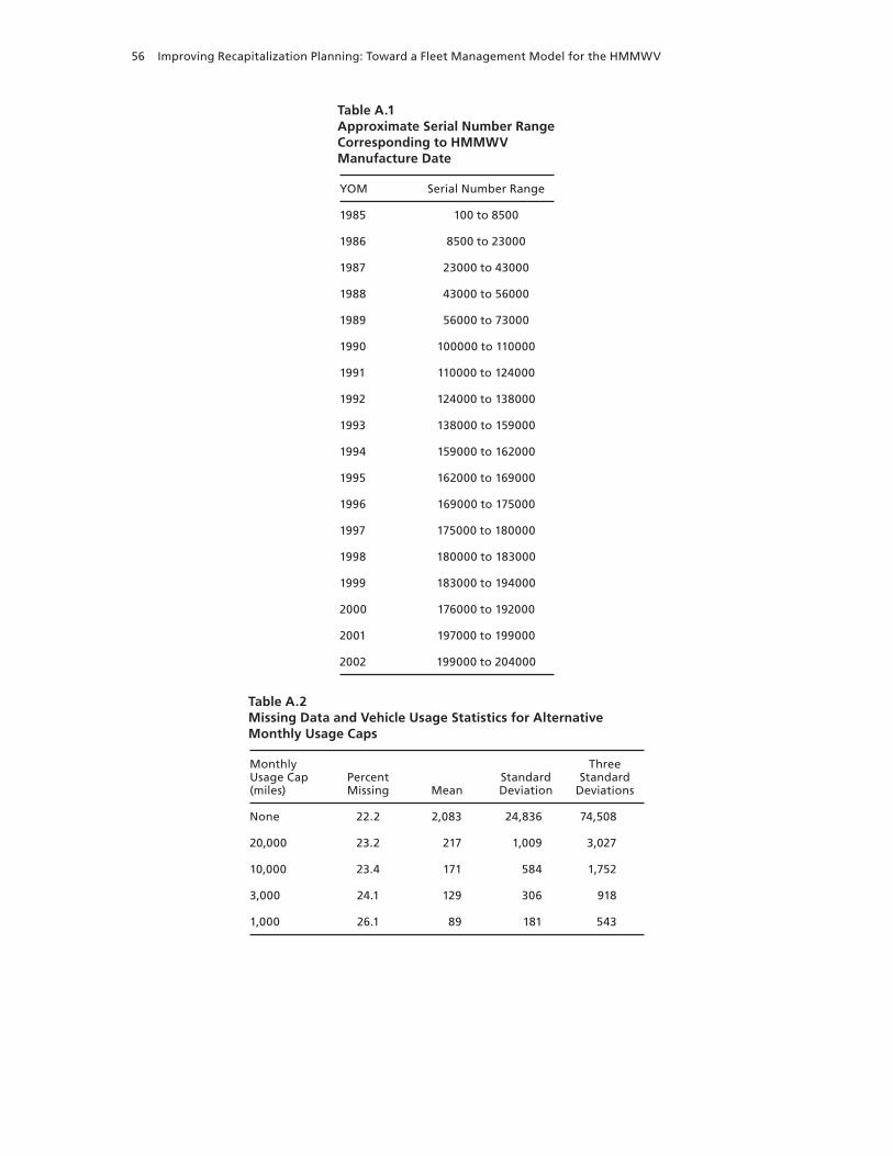
56 Improving Recapitalization Planning: Toward a Fleet Management Model for the HMMWV

Table A.1Approximate Serial Number Range Corresponding to HMMWV Manufacture Date

YOM Serial Number Range

1985 100 to 8500

1986 8500 to 23000

1987 23000 to 43000

1988 43000 to 56000

1989 56000 to 73000

1990 100000 to 110000

1991 110000 to 124000

1992 124000 to 138000

1993 138000 to 159000

1994 159000 to 162000

1995 162000 to 169000

1996 169000 to 175000

1997 175000 to 180000

1998 180000 to 183000

1999 183000 to 194000

2000 176000 to 192000

2001 197000 to 199000

2002 199000 to 204000

Table A.2Missing Data and Vehicle Usage Statistics for Alternative Monthly Usage Caps

Monthly Usage Cap (miles)

Percent Missing Mean

Standard Deviation

Three Standard

Deviations

None 22.2 2,083 24,836 74,508

20,000 23.2 217 1,009 3,027

10,000 23.4 171 584 1,752

3,000 24.1 129 306 918

1,000 26.1 89 181 543

Data Assumptions and Refinements 57

Use of the 3,000-mile cap left some additional vehicles with missing odometer read-ings—and thus missing months of usage data—for their study periods. To minimize the effect of these gaps on our measure of average annual usage, we used simple imputation, substituting reasonable approximations for missing values. When a vehicle was missing usage for a particu-lar month, we computed the average usage of other HMMWVs in the same company, identi-fied by UIC, and replaced the missing value with that company average. If a vehicle still had missing monthly usage (because all vehicles in its company lacked valid usage readings during a particular month), we computed its annual usage by subtracting its minimum odometer reading from its maximum odometer reading during the year.

Related studies on the effects of aging by Peltz et al. (2004a, 2004b) have used the same imputation approach. Peltz et al., 2004a, demonstrated that the use of an alternative, more complex imputation technique (multiple imputation) made little difference in the resulting regression models and the variability of estimates.

Part Order Data

Another data-cleanup procedure involved excluding part orders that were not for true HMMWV parts, even though the equipment (end-item) National Stock Numbers (NSNs) on those part orders corresponded to HMMWV variants. For example, parts from federal supply classes (FSCs) associated with guided missile components, aircraft components, and food preparation were among those we excluded.

Excluding parts with unrelated FSCs, the EDA database recorded the replacement of 178,386 HMMWV parts, representing 5,414 unique NSNs, during the study period. (Note that our analyses did not incorporate all of these part orders, since our sample of HMMWVs did not include all HMMWVs in the EDA data. What our analyses did include were part orders associated with vehicles in our sample during the study period.)

Odometer Readings

When selecting an initial odometer reading to use in our regressions, we needed to ensure that the reading was plausible. As described in Chapter Two, we considered a monthly odometer reading plausible if it (a) did not differ vastly from readings in subsequent months and (b) was not extremely unlikely for a vehicle of the given age. To determine if an odometer reading satis-fied the first criterion, we compared it to six subsequent monthly readings. If it was close to at least one of those readings (i.e., if the two readings differed by no more than N*3,000 miles, where N is the number of months between the two readings), it satisfied the first criterion. We then checked the second criterion. If a reading was less than 10,000*(age of vehicle + 1) and greater than 25*(age of vehicle), it satisfied the second criterion.

58 Improving Recapitalization Planning: Toward a Fleet Management Model for the HMMWV

Repair Costs

Several issues arise in cost-versus-age analyses regarding how to apply prices and credits appro-priately to part orders. One issue is whether to use the prices and credits in effect at the time of the repair (adjusted for inflation) or to use the most current set of prices and credits. The former method captures any growth either in acquisition costs because of part obsolescence or in repair costs as the stock of reparable parts ages, and assumes any trend will continue into the future. The latter method may represent a more accurate picture of current fleet costs.

An additional complication with using then-year prices rather than current-year prices is the Army’s Single Stock Fund (SSF) program. The SSF changed the AWCF point of sale twice during the study period (1999 to 2003)1 and, importantly, was accompanied by a change in price and credit policy in 2001. Prior to FY01, credits for depot-level reparables (DLRs) and field-level reparables (FLRs) depended on local inventory positions and repair programs. Cred-its for unserviceable DLRs not repaired or needed locally were averaged by Materiel Category (MATCAT) and ranged from 50 to 60 percent of purchase price.2 Beginning in FY01, credits for both DLRs and FLRs were based on item-by-item repair costs, although many of them, at least initially, were based on “engineering estimates” or default values set as a percentage of purchase price.3

We chose to use the most recent year, FY03, prices and credits (as of the start of our analysis) because we were primarily interested in estimating current fleet costs. For part credits in particular, we used the item-by-item unserviceable credit rates in the FY03 FEDLOG. As indicated, the use of constant prices and credits avoids any possible inference problems associ-ated with the SSF. And although the use of constant prices and credits could mask any growth in repair costs over time, a plot of average prices and credits for DLRs, FLRs, and consumables used for HMMWV repairs in EDA (see Figure A.1) showed no strong trends in average prices or credits or in the difference between the two.

1 In FY01, during the first phase of SSF, installation-level stocks and General Support repair programs were capitalized into the AWCF. In FY03, during the second phase, Supply Support Activity stocks (also known as Authorized Stockage Lists, or ASLs) were capitalized into the AWCF. These changes also affected the number of part demands that were observed in OSMIS. However, EDA data capture all part orders open for at least one day, even if the part was available in the ASL, so the change in point of sale did not affect these data.2 For example, credits for all tank-automotive DLRs were set at 52.9 percent of purchase price in FY00. Credits for unser-viceable FLRs were set at 80 percent of purchase price if needed and repaired locally, but only 5 percent of purchase price if not repaired or not needed locally.3 For more information, see Pint et al., 2002.

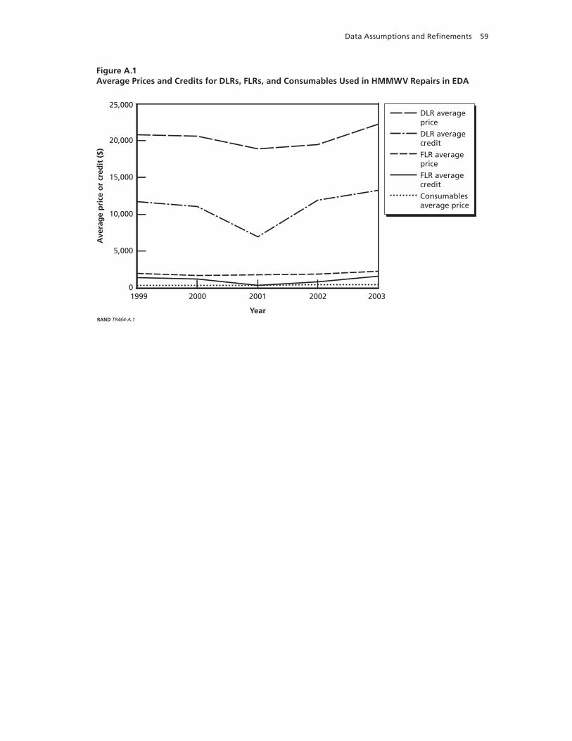
Data Assumptions and Refinements 59

Figure A.1Average Prices and Credits for DLRs, FLRs, and Consumables Used in HMMWV Repairs in EDA

20,000

15,000

10,000

5,000

25,000

20032002200120001999

Year

Ave

rag

e p

rice

or

cred

it (

$)

0

RAND TR464-A.1

DLR averageprice

DLR averagecredit

FLR averageprice

FLR averagecredit

Consumablesaverage price

61

APPENDIX B

Regression Tables and Additional Plots

This appendix contains five regression tables corresponding to the results reported in Chap-ter Three. The first of these, Table B.1, shows results from our logistic regression analysis of the relationship between predictor variables and a dichotomous variable indicating whether a HMMWV did or did not incur NMC repair costs during the study period. Age, usage, and odometer reading had cubic effects, as well as interaction effects, on the positive repair cost indicator, and location and HMMWV variant were also significant predictors.

Table B.2 shows the results of regressing ln(repair costs) on age, usage, initial odometer reading, location, and HMMWV variant for the sample of HMMWVs with positive repair costs. Usage and odometer reading each had log-cubic effects, and age and odometer reading had significant interaction effects on repair costs. Location and HMMWV variant had signifi-cant effects as well.

Figure B.1 illustrates the effect of usage on M998 repair costs (when vehicle age is held constant at 10 years) based on a combination of the regression results in Tables B.1 and B.2. We used Table B.1 to calculate the predicted probabilities of incurring positive repair costs versus usage, and we used Table B.2 to calculate predicted repair costs versus usage for those vehicles with positive repair costs. We then multiplied the two sets of predictions to get pre-dicted repair costs versus usage for all HMMWVs in the sample.

Table B.3 shows results from our logistic-regression analysis of the relationship between predictor variables and a dichotomous variable indicating whether a HMMWV did or did not experience downtime for at least one day during the study period. Age and odometer reading had linear effects; usage had cubic effects. Age and usage had a statistically significant interac-tion effect on the positive downtime indicator, and location and HMMWV variant were also significant predictors.

Table B.4 shows the results of regressing ln(downtime) on age, usage, odometer reading, location, and HMMWV variant for the sample of HMMWVs with positive downtime. Age had a log-linear effect on downtime; usage and odometer reading had log-cubic effects. Sig-nificant interaction effects between age and odometer reading, as well as between usage and odometer reading, were present. Location and HMMWV variant also had significant effects.

Table B.5 shows the results of regressing ln(odometer reading) on age, location, and HMMWV variant. Age had a log-cubic association with the odometer reading of a HMMWV at the start of its study period. Location and variant also had significant associations with odometer reading.

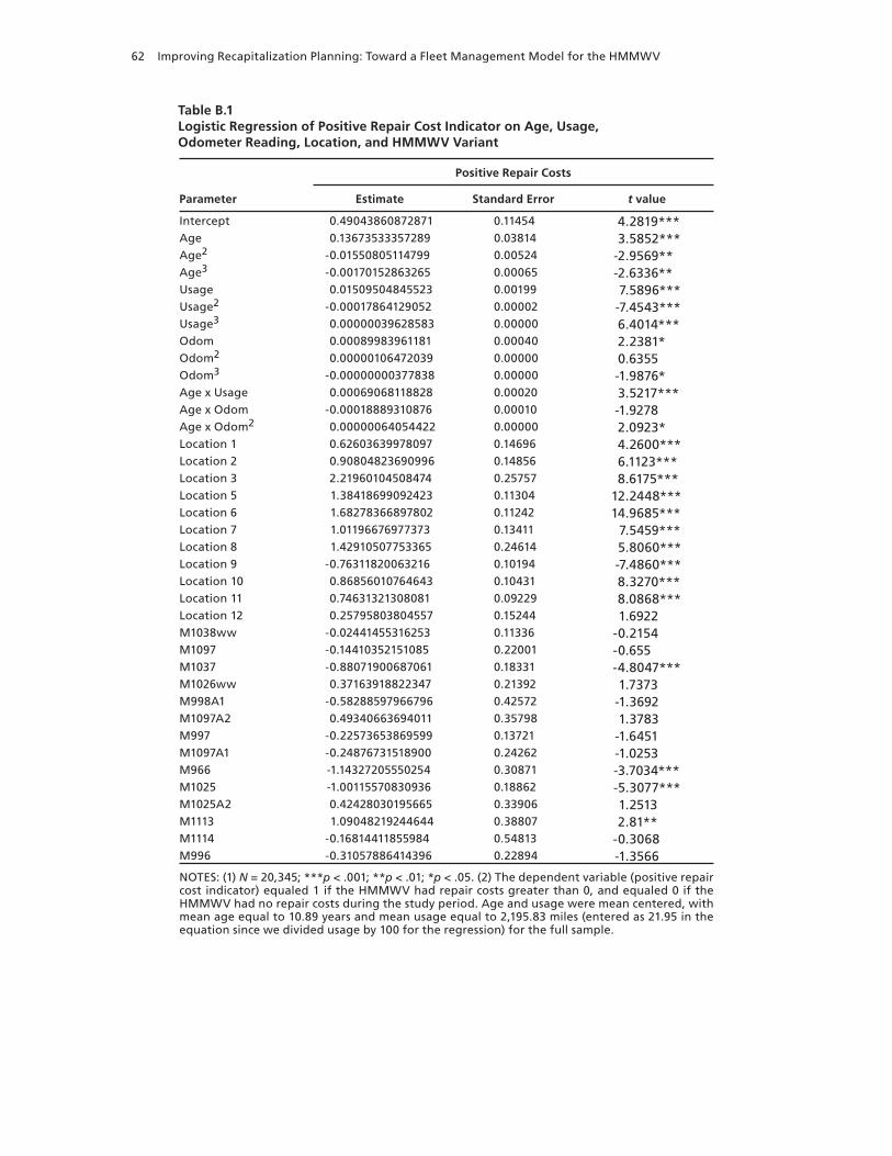
62 Improving Recapitalization Planning: Toward a Fleet Management Model for the HMMWV

Table B.1Logistic Regression of Positive Repair Cost Indicator on Age, Usage, Odometer Reading, Location, and HMMWV Variant

Positive Repair Costs

Parameter Estimate Standard Error t value

Intercept 0.49043860872871 0.11454 4.2819***Age 0.13673533357289 0.03814 3.5852***Age2 -0.01550805114799 0.00524 -2.9569**Age3 -0.00170152863265 0.00065 -2.6336**Usage 0.01509504845523 0.00199 7.5896***Usage2 -0.00017864129052 0.00002 -7.4543***Usage3 0.00000039628583 0.00000 6.4014***Odom 0.00089983961181 0.00040 2.2381*Odom2 0.00000106472039 0.00000 0.6355Odom3 -0.00000000377838 0.00000 -1.9876*Age x Usage 0.00069068118828 0.00020 3.5217***Age x Odom -0.00018889310876 0.00010 -1.9278Age x Odom2 0.00000064054422 0.00000 2.0923*Location 1 0.62603639978097 0.14696 4.2600***Location 2 0.90804823690996 0.14856 6.1123***Location 3 2.21960104508474 0.25757 8.6175***Location 5 1.38418699092423 0.11304 12.2448***Location 6 1.68278366897802 0.11242 14.9685***Location 7 1.01196676977373 0.13411 7.5459***Location 8 1.42910507753365 0.24614 5.8060***Location 9 -0.76311820063216 0.10194 -7.4860***Location 10 0.86856010764643 0.10431 8.3270***Location 11 0.74631321308081 0.09229 8.0868***Location 12 0.25795803804557 0.15244 1.6922M1038ww -0.02441455316253 0.11336 -0.2154M1097 -0.14410352151085 0.22001 -0.655M1037 -0.88071900687061 0.18331 -4.8047***M1026ww 0.37163918822347 0.21392 1.7373M998A1 -0.58288597966796 0.42572 -1.3692M1097A2 0.49340663694011 0.35798 1.3783M997 -0.22573653869599 0.13721 -1.6451M1097A1 -0.24876731518900 0.24262 -1.0253M966 -1.14327205550254 0.30871 -3.7034***M1025 -1.00115570830936 0.18862 -5.3077***M1025A2 0.42428030195665 0.33906 1.2513M1113 1.09048219244644 0.38807 2.81**M1114 -0.16814411855984 0.54813 -0.3068M996 -0.31057886414396 0.22894 -1.3566

NOTES: (1) N = 20,345; ***p < .001; **p < .01; *p < .05. (2) The dependent variable (positive repair cost indicator) equaled 1 if the HMMWV had repair costs greater than 0, and equaled 0 if the HMMWV had no repair costs during the study period. Age and usage were mean centered, with mean age equal to 10.89 years and mean usage equal to 2,195.83 miles (entered as 21.95 in the equation since we divided usage by 100 for the regression) for the full sample.

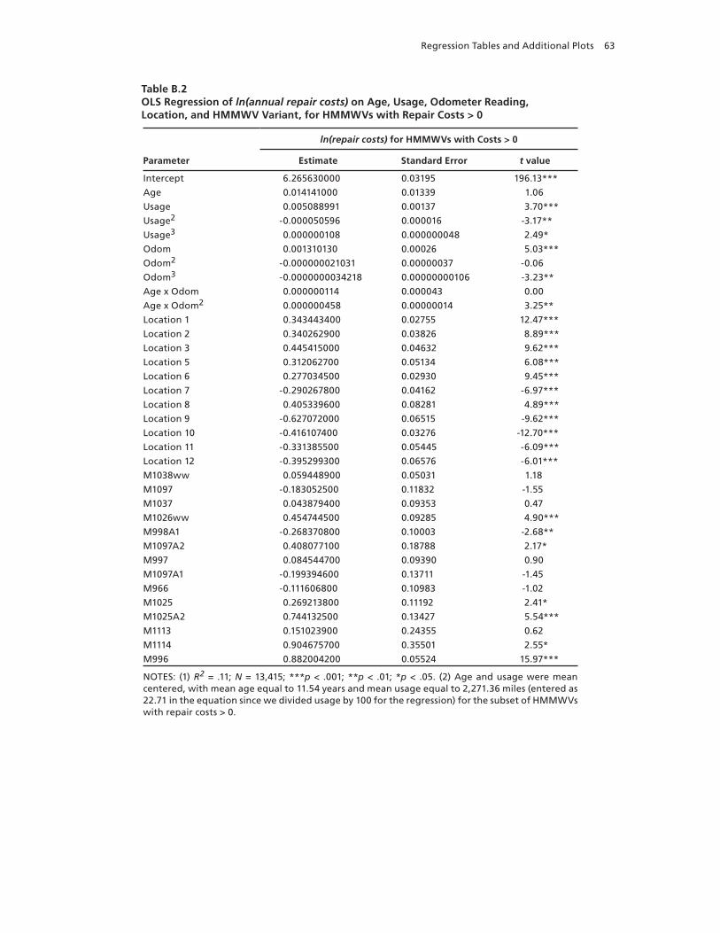
Regression Tables and Additional Plots 63

Table B.2OLS Regression of ln(annual repair costs) on Age, Usage, Odometer Reading, Location, and HMMWV Variant, for HMMWVs with Repair Costs > 0

ln(repair costs) for HMMWVs with Costs > 0

Parameter Estimate Standard Error t value

Intercept 6.265630000 0.03195 196.13***

Age 0.014141000 0.01339 1.06

Usage 0.005088991 0.00137 3.70***

Usage2 -0.000050596 0.000016 -3.17**

Usage3 0.000000108 0.000000048 2.49*

Odom 0.001310130 0.00026 5.03***

Odom2 -0.000000021031 0.00000037 -0.06

Odom3 -0.0000000034218 0.00000000106 -3.23**

Age x Odom 0.000000114 0.000043 0.00

Age x Odom2 0.000000458 0.00000014 3.25**

Location 1 0.343443400 0.02755 12.47***

Location 2 0.340262900 0.03826 8.89***

Location 3 0.445415000 0.04632 9.62***

Location 5 0.312062700 0.05134 6.08***

Location 6 0.277034500 0.02930 9.45***

Location 7 -0.290267800 0.04162 -6.97***

Location 8 0.405339600 0.08281 4.89***

Location 9 -0.627072000 0.06515 -9.62***

Location 10 -0.416107400 0.03276 -12.70***

Location 11 -0.331385500 0.05445 -6.09***

Location 12 -0.395299300 0.06576 -6.01***

M1038ww 0.059448900 0.05031 1.18

M1097 -0.183052500 0.11832 -1.55

M1037 0.043879400 0.09353 0.47

M1026ww 0.454744500 0.09285 4.90***

M998A1 -0.268370800 0.10003 -2.68**

M1097A2 0.408077100 0.18788 2.17*

M997 0.084544700 0.09390 0.90

M1097A1 -0.199394600 0.13711 -1.45

M966 -0.111606800 0.10983 -1.02

M1025 0.269213800 0.11192 2.41*

M1025A2 0.744132500 0.13427 5.54***

M1113 0.151023900 0.24355 0.62

M1114 0.904675700 0.35501 2.55*

M996 0.882004200 0.05524 15.97***

NOTES: (1) R2 = .11; N = 13,415; ***p < .001; **p < .01; *p < .05. (2) Age and usage were mean centered, with mean age equal to 11.54 years and mean usage equal to 2,271.36 miles (entered as 22.71 in the equation since we divided usage by 100 for the regression) for the subset of HMMWVs with repair costs > 0.

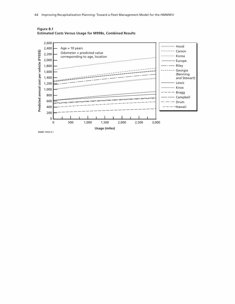
64 Improving Recapitalization Planning: Toward a Fleet Management Model for the HMMWV

Figure B.1Estimated Costs Versus Usage for M998s, Combined Results

600

400

200

2,600

3,0005000

Usage (miles)

Pred

icte

d a

nn

ual

co

st p

er v

ehic

le (

FY03

$)

0

2,400

2,200

2,000

1,800

1,600

1,400

1,200

1,000

800

RAND TR464-B.1

2,5002,0001,5001,000

Hood

Carson

Korea

Europe

Riley

Georgia(Benningand Stewart)

Lewis

Knox

Bragg

Campbell

Drum

Hawaii

Age = 10 yearsOdometer = predicted valuecorresponding to age, location

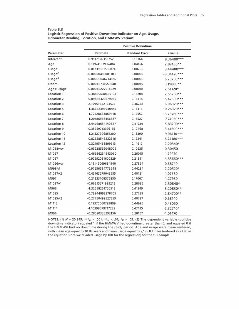
Regression Tables and Additional Plots 65

Table B.3Logistic Regression of Positive Downtime Indicator on Age, Usage, Odometer Reading, Location, and HMMWV Variant

Positive Downtime

Parameter Estimate Standard Error t value

Intercept 0.95179263537529 0.10164 9.36400***Age 0.11974167937484 0.04166 2.87430**Usage 0.01739881585874 0.00206 8.44400***Usage2 -0.00020418081103 0.00002 -8.31420***Usage3 0.00000046714186 0.00000 6.73750***Odom 0.00046731559240 0.00015 3.19080**Age x Usage 0.00045227514229 0.00018 2.51120*Location 1 0.38889640655103 0.15204 2.55780**Location 2 0.89886329279089 0.16418 5.47500***Location 3 2.19959642123574 0.36278 6.06320***Location 5 1.36642393940447 0.13314 10.26320***Location 6 1.72428633869418 0.12552 13.73760***Location 7 1.20186958456587 0.15527 7.74030***Location 8 2.44768654140827 0.41934 5.83700***Location 9 -0.35759713376155 0.10468 -3.41600***Location 10 1.21327906851200 0.13390 9.06110***Location 11 0.82528546232616 0.12241 6.74180***Location 12 0.32195438899513 0.14612 2.20340*M1038ww -0.03238562048005 0.10635 -0.30450M1097 -0.46636234943060 0.26015 -1.79270M1037 -0.92592081600329 0.21351 -4.33660***M1026ww 0.19146069684940 0.27854 0.68740M998A1 -0.97656584773648 0.44284 -2.20520*M1097A2 -0.43163279043555 0.40121 -1.07580M997 0.21833108575850 0.17067 1.27930M1097A1 -0.66215571999218 0.28685 -2.30840*M966 -1.32658261750513 0.41349 -3.20830**M1025 -0.78944892278705 0.27729 -2.84700**M1025A2 -0.27750499527359 0.40727 -0.68140M1113 0.19370060793899 0.44995 0.43050M1114 -1.10398579717229 0.47435 -2.32740*M996 -0.28520338292156 0.28107 -1.01470

NOTES: (1) N = 20,345; ***p < .001; **p < .01; *p < .05. (2) The dependent variable (positive downtime indicator) equaled 1 if the HMMWV had downtime greater than 0, and equaled 0 if the HMMWV had no downtime during the study period. Age and usage were mean centered, with mean age equal to 10.89 years and mean usage equal to 2,195.83 miles (entered as 21.95 in the equation since we divided usage by 100 for the regression) for the full sample.

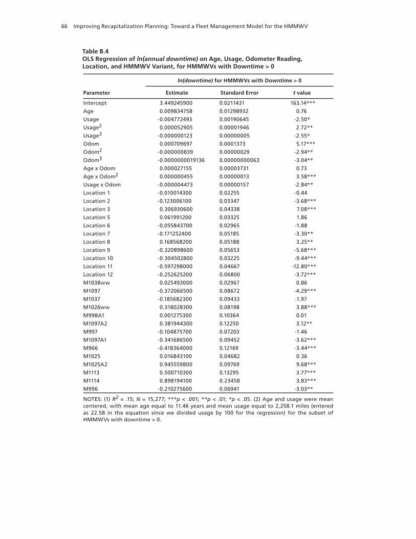
66 Improving Recapitalization Planning: Toward a Fleet Management Model for the HMMWV

Table B.4OLS Regression of ln(annual downtime) on Age, Usage, Odometer Reading, Location, and HMMWV Variant, for HMMWVs with Downtime > 0

ln(downtime) for HMMWVs with Downtime > 0

Parameter Estimate Standard Error t value

Intercept 3.449245900 0.0211431 163.14***

Age 0.009834758 0.01298932 0.76

Usage -0.004772493 0.00190645 -2.50*

Usage2 0.000052905 0.00001946 2.72**

Usage3 -0.000000123 0.00000005 -2.55*

Odom 0.000709697 0.0001373 5.17***

Odom2 -0.000000839 0.00000029 -2.94**

Odom3 -0.0000000019136 0.00000000063 -3.04**

Age x Odom 0.000027155 0.00003731 0.73

Age x Odom2 0.000000455 0.00000013 3.58***

Usage x Odom -0.000004473 0.00000157 -2.84**

Location 1 -0.010014300 0.02255 -0.44

Location 2 -0.123006100 0.03347 -3.68***

Location 3 0.306930600 0.04338 7.08***

Location 5 0.061991200 0.03325 1.86

Location 6 -0.055843700 0.02965 -1.88

Location 7 -0.171252400 0.05185 -3.30**

Location 8 0.168568200 0.05188 3.25**

Location 9 -0.320898600 0.05653 -5.68***

Location 10 -0.304502800 0.03225 -9.44***

Location 11 -0.597298000 0.04667 -12.80***

Location 12 -0.252625200 0.06800 -3.72***

M1038ww 0.025493000 0.02967 0.86

M1097 -0.372066500 0.08672 -4.29***

M1037 -0.185682300 0.09433 -1.97

M1026ww 0.318028300 0.08198 3.88***

M998A1 0.001275300 0.10364 0.01

M1097A2 0.381944300 0.12250 3.12**

M997 -0.104875700 0.07203 -1.46

M1097A1 -0.341686500 0.09452 -3.62***

M966 -0.418364000 0.12169 -3.44***

M1025 0.016843100 0.04682 0.36

M1025A2 0.945559800 0.09769 9.68***

M1113 0.500710300 0.13295 3.77***

M1114 0.898194100 0.23458 3.83***

M996 -0.210275600 0.06941 -3.03**

NOTES: (1) R2 = .15; N = 15,277; ***p < .001; **p < .01; *p < .05. (2) Age and usage were mean centered, with mean age equal to 11.46 years and mean usage equal to 2,258.1 miles (entered as 22.58 in the equation since we divided usage by 100 for the regression) for the subset of HMMWVs with downtime > 0.

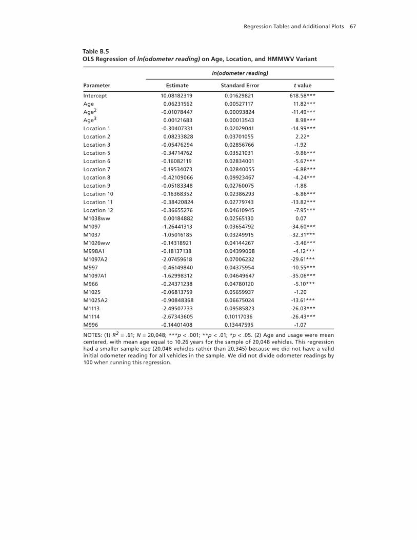
Regression Tables and Additional Plots 67

Table B.5OLS Regression of ln(odometer reading) on Age, Location, and HMMWV Variant

ln(odometer reading)

Parameter Estimate Standard Error t value

Intercept 10.08182319 0.01629821 618.58***

Age 0.06231562 0.00527117 11.82***

Age2 -0.01078447 0.00093824 -11.49***

Age3 0.00121683 0.00013543 8.98***

Location 1 -0.30407331 0.02029041 -14.99***

Location 2 0.08233828 0.03701055 2.22*

Location 3 -0.05476294 0.02856766 -1.92

Location 5 -0.34714762 0.03521031 -9.86***

Location 6 -0.16082119 0.02834001 -5.67***

Location 7 -0.19534073 0.02840055 -6.88***

Location 8 -0.42109066 0.09923467 -4.24***

Location 9 -0.05183348 0.02760075 -1.88

Location 10 -0.16368352 0.02386293 -6.86***

Location 11 -0.38420824 0.02779743 -13.82***

Location 12 -0.36655276 0.04610945 -7.95***

M1038ww 0.00184882 0.02565130 0.07

M1097 -1.26441313 0.03654792 -34.60***

M1037 -1.05016185 0.03249915 -32.31***

M1026ww -0.14318921 0.04144267 -3.46***

M998A1 -0.18137138 0.04399008 -4.12***

M1097A2 -2.07459618 0.07006232 -29.61***

M997 -0.46149840 0.04375954 -10.55***

M1097A1 -1.62998312 0.04649647 -35.06***

M966 -0.24371238 0.04780120 -5.10***

M1025 -0.06813759 0.05659937 -1.20

M1025A2 -0.90848368 0.06675024 -13.61***

M1113 -2.49507733 0.09585823 -26.03***

M1114 -2.67343605 0.10117036 -26.43***

M996 -0.14401408 0.13447595 -1.07

NOTES: (1) R2 = .61; N = 20,048; ***p < .001; **p < .01; *p < .05. (2) Age and usage were mean centered, with mean age equal to 10.26 years for the sample of 20,048 vehicles. This regression had a smaller sample size (20,048 vehicles rather than 20,345) because we did not have a valid initial odometer reading for all vehicles in the sample. We did not divide odometer readings by 100 when running this regression.

69

References

Aiken, Leona S., Stephen G. West, and Raymond R. Reno, Multiple Regression: Testing and Interpreting Interactions, Newbury Park, Calif.: Sage Publications, 1991.

Apollonio, D. E., and Raymond J. La Raja, “Who Gave Soft Money? The Effect of Interest Group Resources on Political Contributions,” The Journal of Politics, Vol. 66, No. 4, 2004, pp. 1134–1154.

Begg, Melissa D., and Michael K. Parides, “Separation of Individual-level and Cluster-level Covariate Effects in Regression Analysis of Correlated Data,” Statistics in Medicine, Vol. 22, 2003, pp. 2591–2602.

Berglund, Patricia A., “Analysis of Complex Sample Survey Data Using the SURVEYMEANS and SURVEYREG Procedures and Macro Coding,” Paper 263-27, SUGI (SAS Users Group International) Proceedings, Orlando, Florida, April 14–17, 2002. As of December 19, 2006: http://www2.sas.com/proceedings/sugi27/p263-27.pdf

Bernhard, Richard H., “Improving the Economic Logic Underlying Replacement Age Decisions for Municipal Garbage Trucks: Case Study,” The Engineering Economist, Vol. 35, No. 2, 1990, pp. 129–148.

Department of the Army, Army Working Capital Fund Fiscal Year (FY) 2004/2005 Biennial Budget Estimates, February 2003. As of December 7, 2006: http://www.asafm.army.mil/budget/fybm/fy04-05/awcf.pdf

Diehr, P., D. Yanez, A. Ash, and M. Hornbrook, “Methods for Analyzing Health Care Utilization and Costs,” Annual Review of Public Health, Vol. 20, 1999, pp. 125–144.

Dietz, Dennis C., and Paul A. Katz, “US WEST Implements a Cogent Analytical Model for Optimal Vehicle Replacement,” Interfaces, Vol. 31, No. 5, 2001, pp. 65–73.

Duan, Naihua, “Smearing Estimate: A Nonparametric Retransformation Method,” Journal of the American Statistical Association, Vol. 78, No. 383, 1983, pp. 605–610.

East, Allen C., Planning Army Recapitalization Investment Strategies, Fort Belvoir, Virginia: Center for Army Analysis, 2002.

Fan, Carol, Eric Peltz, and Lisa Colabella, The Effects of Equipment Age on Spare Parts Costs: A Study of M1 Tanks, TR-286-A, Santa Monica, Calif.: RAND Corporation, 2005. As of February 27, 2006: http://www.rand.org/pubs/technical_reports/TR286/

Gansler, Jacques S., “Defense Logistics Reengineering Initiatives: Hearing Before the Military Readiness Subcommittee of the Committee on Armed Services, House of Representatives, One Hundred Sixth Congress, Second Session,” June 27, 2000. As of April 17, 2007: http://armedservices.house.gov/comdocs/testimony/106thcongress/00-06-27gansler.html

GlobalSecurity.org, “High Mobility Multipurpose Wheeled Vehicle (HMMWV),” undated. As of February 27, 2006: http://www.globalsecurity.org/military/systems/ground/hmmwv.htm

Gourley, Scott, “HMMWV: The Art of Military Progress,” The Officer, 2002, pp. 28–29.

70 Improving Recapitalization Planning: Toward a Fleet Management Model for the HMMWV

Griffin, Benjamin S., “Testimony of Lieutenant General Benjamin Griffin, Deputy Chief for Plans and Programs (G8), United States Army, Before the House Armed Services Committee, Subcommittee on Tactical Air and Land Forces, United States House of Representatives, Regarding Future Combat System and Force Protection Initiatives,” April 1, 2004. As of April 17, 2007: http://armedservices.house.gov/comdocs/openingstatementsandpressreleases/108thcongress/04-04-01griffin.html

Harvey, Francis J., “A Letter to the Soldiers of the U.S. Army,” Army Well-Being, Vol. 3, No. 1, 2005. As of March 16, 2006: http://www.wblo.org/data/spring_05.pdf

Held, Tom, Eric Peltz, and Melvin Wolff, “Benchmarking of Army Fleet Management, Volume 1: Comparison to Public Sector Fleet Performance and Practices,” unpublished RAND research, December 2004.

Held, Tom, and Melvin Wolff, “How Increased Reliability Can Be Achieved by Effective Preventive Maintenance,” unpublished RAND research, November 2004.

Henke, Serina, “Shingo Prize Site Visit,” Kenny Letter, Vol. 39, Nos. 3–6, March–June 2006. As of October 12, 2006: http://www.letterkenny.army.mil/PAO/March-June%20Kennyletter.pdf

Joyner, Michael T., ed., Managing Public Equipment, 2nd edition, Kansas City, Missouri: American Public Works Association, August 2000.

Kapur, Kanika, Alexander S. Young, and Dennis Murata, “Risk Adjustment for High Utilizers of Public Mental Health Care,” The Journal of Mental Health Policy and Economics, Vol. 3, No. 3, 2000, pp. 129–137.

Keles, Pinar, and Joseph C. Hartman, “Case Study: Bus Fleet Replacement,” The Engineering Economist, Vol. 49, No. 3, 2004, pp. 253–278.

Kiley, Gregory T., and John Skeen, The Effects of Aging on the Costs of Operating and Maintaining Military Equipment, Washington, D.C.: Congressional Budget Office, 2001. As of February 27, 2006: http://www.cbo.gov/ftpdocs/29xx/doc2982/AgingCostsO&M.pdf

Lauria, Paul, “When Vehicle Replacement Budgets Shrink: Think Outside the Box,” Fleet Financials, July/August 2002, pp. 32–38. As of July 7, 2006: http://www.mercury-assoc.com/resources/fleet-financing-alt-1.pdf

Liu, Korbin, Sharon K. Long, and Krista Dowling, “Medicare Interim Payment System’s Impact on Medicare Home Health Utilization,” Health Care Financing Review, Vol. 25, No. 1, 2003, pp. 81–97. As of April 17, 2007: http://www.cms.hhs.gov/HealthCareFinancingReview/Downloads/03fallpg81.pdf

Lucko, Gunnar, A Statistical Analysis and Model of the Residual Value of Different Types of Heavy Construction Equipment, Ph.D. dissertation, Virginia Polytechnic Institute and State University, December 2003.

Lundborg, Petter, and Björn Lindgren, “Do They Know What They Are Doing? Risk Perceptions and Smoking Behaviour Among Swedish Teenagers,” Journal of Risk and Uncertainty, Vol. 28, No. 3, 2004, pp. 261–286.

Newhouse, Joseph P., “Is Competition the Answer?” Journal of Health Economics, Vol. 1, No. 1, 1982, pp. 109–116.

Office of Management and Budget of the Executive Office of the President of the United States of America, Memorandum for Heads of Executive Departments and Establishments; Subject: Guidelines and Discount Rates for Benefit-Cost Analysis of Federal Programs, Circular No. A-94 Revised (Transmittal Memo No. 64), Washington, D.C.: Office of Management and Budget, October 29, 1992. As of March 19, 2007: http://www.whitehouse.gov/omb/circulars/a094/a094.html#8

Office of Management and Budget of the Executive Office of the President of the United States of America, “Discount Rates for Cost-Effectiveness, Lease Purchase, and Related Analyses,” Appendix C of OMB Circular

References 71

No. A-94, Washington, D.C.: Office of Management and Budget, 2006. As of June 9, 2007: http://www.whitehouse.gov/omb/circulars/a094/dischist-2007.pdf

Olenginski, S. J., Recapitalization and Modernization (RECAP/MOD) Analysis, CAA-R-05-24, Fort Belvoir, Virginia: Center for Army Analysis, 2005.

OMB—see Office of Management and Budget of the Executive Office of the President of the United States of America.

Owen, Randy, “Cost Understanding and Awareness: Key Steps in Having a Cost-Competitive Fleet Management Program,” APWA Reporter, August 2004, pp. 35–37. As of July 7, 2006: http://www.mercury-assoc.com/resources/cost-competitive-fleet-management.pdf

Pasta, David J., and Miriam G. Cisternas, “Estimating Standard Errors for CLASS Variables in Generalized Linear Models Using PROC IML,” Paper 264-28, Proceedings of the Twenty-Eighth Annual SAS Users Group International Conference, Cary, North Carolina: SAS Institute, Inc., 2003. As of March 16, 2006: http://www2.sas.com/proceedings/sugi28/264-28.pdf

Peltz, Eric, Patricia Boren, Marc Robbins, and Melvin Wolff, Diagnosing the Army’s Equipment Readiness: The Equipment Downtime Analyzer, MR-1481-A, Santa Monica, Calif.: RAND Corporation, 2002. As of February 27, 2006: http://www.rand.org/pubs/monograph_reports/MR1481/

Peltz, Eric, Lisa Colabella, Brian Williams, and Patricia Boren, The Effects of Equipment Age on Mission-Critical Failure Rates: A Study of M1 Tanks, MR-1789-A, Santa Monica, Calif.: RAND Corporation, 2004a. As of February 27, 2006: http://www.rand.org/pubs/monograph_reports/MR1789/

Peltz, Eric, Lisa Colabella, Brian Williams, Patricia Boren, and Aimee Bower, “Predicting Mission-Critical Failures of Army Ground Systems: Age, Usage, and Location Effects,” unpublished RAND research, 2004b.

Pint, Ellen M., Marygail K. Brauner, John R. Bondanella, Daniel A. Relles, and Paul Steinberg, Right Price, Fair Credit: Criteria to Improve Financial Incentives for Army Logistics Decisions, MR-1150-A, Santa Monica, Calif.: RAND Corporation, 2002. As of February 27, 2006: http://www.rand.org/pubs/monograph_reports/MR1150/

Primo, David M., Matthew L. Jacobsmeier, and Jeffrey Milyo, “Estimating the Impact of State Policies and Institutions with Mixed-Level Data,” Working Paper No. 0603, University of Missouri Department of Economics, February 2006. As of December 19, 2006: http://economics.missouri.edu/Working_Paper_Series/2006/wp0603_milyo.pdf

Simberg, Henry, “AMSAA Sample Data Collection System Usage/Parts Replacement Analysis, Operation Iraqi Freedom,” Briefing, August 2005.

Sturm, Roland, “How Does Risk Sharing Between Employers and a Managed Behavioral Health Organization Affect Mental Health Care?” Health Services Research, Vol. 35, No. 4, 2000, pp. 761–776.

Sutton, Rod, “Use Benchmarks to Judge Shop Overhead,” Construction Equipment, April 1, 2005a. As of December 8, 2006: http://www.constructionequipment.com/article/CA515040.html

Sutton, Rod, “Shop Overhead Data,” Construction Equipment, June 1, 2005b. As of December 8, 2006: http://www.constructionequipment.com/article/CA605567.html

U.S. Army Force Management Support Agency, Manpower Requirements Criteria (MARC), “How To” Procedures Guide, Chapter 2, “MARC Process Procedures Overview,” October 1, 2005. As of December 19, 2006: https://webtaads.belvoir.army.mil

U.S. Government Accountability Office (GAO). Military Readiness: DOD Needs to Identify and Address Gaps and Potential Risks in Program Strategies and Funding Priorities for Selected Equipment, GAO-06-141,

72 Improving Recapitalization Planning: Toward a Fleet Management Model for the HMMWV

Washington, D.C., 2005. As of October 5, 2006: http://www.gao.gov/new.items/d06141.pdf

Vorster, Mike, “Equipment Executive: How to Estimate Market Value,” Construction Equipment, June 1, 2004. As of July 10, 2006: http://www.constructionequipment.com/article/CA457578.html

Vorster, Mike, “Equipment Executive: The Residual-Value Grid,” Construction Equipment, May 1, 2006. As of July 10, 2006: http://www.constructionequipment.com/article/CA6329615.html

“Washington Report,” Army Magazine, Vol. 54, No. 3, 2004. As of February 27, 2006: http://www.ausa.org/webpub/DeptArmyMagazine.nsf/byid/CCRN-6CCSC7

Worley, Lorna, “Revolutionizing Logistics Information Support for the Warfighter,” Army Logistician: Professional Bulletin of United States Army Logistics, Vol. 33, No. 1, 2001, pp. 13–15. As of February 27, 2006: http://www.almc.army.mil/alog/issues/JanFeb01/2001jan_feb/artp13_01jf.pdf