
Improving Patient Transportation Performance by Developing … · Abstract Improving Patient...
105
Improving Patient Transportation Performance by Developing and Implementing a Generic Simulation Model by Carly Henshaw A thesis submitted in conformity with the requirements for the degree of Master of Applied Science Graduate Department of Mechanical and Industrial Engineering University of Toronto c Copyright 2015 by Carly Henshaw
Transcript of Improving Patient Transportation Performance by Developing … · Abstract Improving Patient...

Improving Patient Transportation Performance byDeveloping and Implementing a Generic Simulation Model
by
Carly Henshaw
A thesis submitted in conformity with the requirementsfor the degree of Master of Applied Science
Graduate Department of Mechanical and Industrial EngineeringUniversity of Toronto
c© Copyright 2015 by Carly Henshaw

Abstract
Improving Patient Transportation Performance by Developing and Implementing a
Generic Simulation Model
Carly Henshaw
Master of Applied Science
Graduate Department of Mechanical and Industrial Engineering
University of Toronto
2015
Patient transportation is a department in hospitals responsible for transporting patients
or items from one point of a hospital to another. Without proper coordination of this
department, patient flow and hospitals functions are impacted. With the end goal of
improving portering efficiency, this thesis has two main objectives: the first is to develop
a generic portering simulation model; the second is to test the model’s generality by
using it as a decision support tool to improve porter performance at North York General
Hospital and Juravinski Hospital and Cancer Centre.
Once the simulation models were validated, improvement scenarios were tested. These
scenarios were developed in collaboration with the hospitals involved. The result of
this scenario testing yielded an improvement in key performance indicators including:
dispatch time, turnaround time and percentage of tasks completed within the target time.
This evidence-based research will be used to support future portering improvements.
ii

Acknowledgements
I would like to thank my supervisor, Professor Michael Carter for his encouragement,
patience and expertise during our meetings and throughout various milestones in my
research. If I was ever confused on what to do next or how I could improve my research,
he always gave me direction and reassurance.
I would also like to thank my lab colleagues for all their guidance as I settled into
my research, as well as their discussions and input regarding my research. Over the two
summer semesters of my Master’s, I had the help of high school student Christian Mele,
who I would like to thank for his dedication and eagerness towards my project.
From North York General Hospital, I would like to thank James Ibbott who shared
so much enthusiasm for my project and overall passion for improving healthcare, which
was very inspiring for me as I looked towards a career in healthcare. I appreciated his
leadership and patience throughout the two years we worked together. I would also like
to thank the portering manager, Kenny Paiva, for his commitment to my project.
At Juravinski Hospital and Cancer Center, from the Customer Support Services de-
partment, I would like to thank portering managers Frank Amatangelo and Ian Deans,
as well as site manager David DiSimoni for sharing their opinions and ideas throughout
this project. I would also like to thank Corey Stark for guiding me at the beginning of
this project and for sharing his technical expertise. Finally, I would like to thank Talha
Hussain for coordinating this project and offering me both research and career related
advice.
Lastly, I would like to thank my parents for always supporting and encouraging me
to never give up, and for taking the time to review some of my work. I would also like
to thank Ryan for his valuable feedback and opinions throughout the past two years.
iii

Contents
1 Introduction 1
1.1 Background . . . . . . . . . . . . . . . . . . . . . . . . . . . . . . . . . . 2
1.1.1 North York General Hospital . . . . . . . . . . . . . . . . . . . . . 3
1.1.2 Juravinski Hospital and Cancer Centre . . . . . . . . . . . . . . . 6
1.2 Problem Definition . . . . . . . . . . . . . . . . . . . . . . . . . . . . . . 9
1.3 Research Objectives . . . . . . . . . . . . . . . . . . . . . . . . . . . . . . 10
2 Literature Review 12
2.1 Root Causes for Patient Flow Delays . . . . . . . . . . . . . . . . . . . . 12
2.2 Adaptation of New Technology . . . . . . . . . . . . . . . . . . . . . . . 13
2.3 Adaptation of Qualitative Techniques . . . . . . . . . . . . . . . . . . . . 14
2.4 Optimization of the Porter Schedule . . . . . . . . . . . . . . . . . . . . . 16
2.5 Comparison to another Process . . . . . . . . . . . . . . . . . . . . . . . 18
2.6 Discrete Event Simulation . . . . . . . . . . . . . . . . . . . . . . . . . . 19
2.7 Generic Simulation Models . . . . . . . . . . . . . . . . . . . . . . . . . . 21
3 Methodology 23
iv

3.1 Generic Simulation Model Development . . . . . . . . . . . . . . . . . . . 23
3.1.1 Model Design . . . . . . . . . . . . . . . . . . . . . . . . . . . . . 24
3.1.2 Inputs . . . . . . . . . . . . . . . . . . . . . . . . . . . . . . . . . 26
3.1.3 Outputs . . . . . . . . . . . . . . . . . . . . . . . . . . . . . . . . 28
3.2 Simulation Model: NYGH . . . . . . . . . . . . . . . . . . . . . . . . . . 30
3.2.1 Data Analysis . . . . . . . . . . . . . . . . . . . . . . . . . . . . . 31
3.2.2 Inputs . . . . . . . . . . . . . . . . . . . . . . . . . . . . . . . . . 32
3.2.3 Assumptions and Limitations . . . . . . . . . . . . . . . . . . . . 36
3.2.4 Validation . . . . . . . . . . . . . . . . . . . . . . . . . . . . . . . 38
3.3 Simulation Model: JHCC . . . . . . . . . . . . . . . . . . . . . . . . . . . 42
3.3.1 Data Analysis . . . . . . . . . . . . . . . . . . . . . . . . . . . . . 42
3.3.2 Inputs . . . . . . . . . . . . . . . . . . . . . . . . . . . . . . . . . 42
3.3.3 Assumptions and Limitations . . . . . . . . . . . . . . . . . . . . 47
3.3.4 Validation . . . . . . . . . . . . . . . . . . . . . . . . . . . . . . . 48
4 Scenario Testing 53
4.1 Improvement Scenarios: NYGH . . . . . . . . . . . . . . . . . . . . . . . 53
4.2 Improvement Scenarios: JHCC . . . . . . . . . . . . . . . . . . . . . . . 59
4.3 Sensitivity Analysis: NYGH . . . . . . . . . . . . . . . . . . . . . . . . . 64
4.4 Sensitivity Analysis: JHCC . . . . . . . . . . . . . . . . . . . . . . . . . 65
5 Results 66
5.1 Simulation Results: NYGH . . . . . . . . . . . . . . . . . . . . . . . . . 66
v

5.2 Simulation Results: JHCC . . . . . . . . . . . . . . . . . . . . . . . . . . 72
6 Conclusion 77
7 Future Research 79
References 80
A Process Maps for Dispatching Processes 86
A.1 Process Maps . . . . . . . . . . . . . . . . . . . . . . . . . . . . . . . . . 86
B Porter Shift Schedules 88
B.1 Porter Schedule: NYGH . . . . . . . . . . . . . . . . . . . . . . . . . . . 88
B.2 Porter Schedule: JHCC . . . . . . . . . . . . . . . . . . . . . . . . . . . . 88
C Further Scenario Testing Results 91
C.1 Further Results: NYGH . . . . . . . . . . . . . . . . . . . . . . . . . . . 91
C.2 Further Results: JHCC . . . . . . . . . . . . . . . . . . . . . . . . . . . . 91
vi
List of Tables
1.1 Evaluation of NYGH’s Porter Performance . . . . . . . . . . . . . . . . . 10
1.2 Evaluation of JHCC’s Porter Performance . . . . . . . . . . . . . . . . . 11
3.1 Task Types Measured for each Performance Metric . . . . . . . . . . . . 30
3.2 Task Breakdown at NYGH . . . . . . . . . . . . . . . . . . . . . . . . . . 33
3.3 Personal Response Times at NYGH . . . . . . . . . . . . . . . . . . . . . 35
3.4 Task Times at NYGH . . . . . . . . . . . . . . . . . . . . . . . . . . . . 35
3.5 Cancellation Rates at NYGH . . . . . . . . . . . . . . . . . . . . . . . . 36
3.6 Task Breakdown at JHCC . . . . . . . . . . . . . . . . . . . . . . . . . . 43
3.7 Priority Level Analysis . . . . . . . . . . . . . . . . . . . . . . . . . . . . 44
3.8 Arrival Minutes at JHCC . . . . . . . . . . . . . . . . . . . . . . . . . . . 46
3.9 Patient Minutes at JHCC . . . . . . . . . . . . . . . . . . . . . . . . . . 46
3.10 Cancellation Rates at JHCC . . . . . . . . . . . . . . . . . . . . . . . . . 47
4.1 Adding Weekday Shifts . . . . . . . . . . . . . . . . . . . . . . . . . . . . 54
4.2 Adding Weekend Shifts . . . . . . . . . . . . . . . . . . . . . . . . . . . . 55
4.3 Changing Weekday Shifts . . . . . . . . . . . . . . . . . . . . . . . . . . 57
vii

4.4 Changing Weekend Shifts . . . . . . . . . . . . . . . . . . . . . . . . . . 57
4.5 Scenario 8 Improvements . . . . . . . . . . . . . . . . . . . . . . . . . . . 59
4.6 Adding Weekday Shifts . . . . . . . . . . . . . . . . . . . . . . . . . . . . 60
4.7 Adding Weekend Shifts . . . . . . . . . . . . . . . . . . . . . . . . . . . . 61
4.8 Changing Weekday Shifts . . . . . . . . . . . . . . . . . . . . . . . . . . 61
4.9 Changing Weekend Shifts . . . . . . . . . . . . . . . . . . . . . . . . . . 62
4.10 Scenario 6 Improvements . . . . . . . . . . . . . . . . . . . . . . . . . . . 63
4.11 Sensitivity Analysis Scenarios: NYGH . . . . . . . . . . . . . . . . . . . 64
4.12 Sensitivity Analysis Scenarios: JHCC . . . . . . . . . . . . . . . . . . . . 65
5.1 NYGH Scenario Legend . . . . . . . . . . . . . . . . . . . . . . . . . . . 67
5.2 NYGH Confidence Intervals for Weekday Results . . . . . . . . . . . . . 68
5.3 KPIs resulting from Simulation . . . . . . . . . . . . . . . . . . . . . . . 69
5.4 JHCC Scenario Legend . . . . . . . . . . . . . . . . . . . . . . . . . . . . 73
5.5 JHCC Confidence Intervals for Weekday Results . . . . . . . . . . . . . . 74
5.6 KPIs resulting from Simulation . . . . . . . . . . . . . . . . . . . . . . . 74
C.1 NYGH Confidence Intervals for Weekend Results . . . . . . . . . . . . . 92
C.2 JHCC Confidence Intervals for Weekend Results . . . . . . . . . . . . . . 92
viii

List of Figures
1.1 NYGH Arrival Analysis . . . . . . . . . . . . . . . . . . . . . . . . . . . 4
1.2 Timeline of Porter Process at NYGH . . . . . . . . . . . . . . . . . . . . 5
1.3 NYGH Porter Process Map . . . . . . . . . . . . . . . . . . . . . . . . . 5
1.4 JHCC Arrival Analysis . . . . . . . . . . . . . . . . . . . . . . . . . . . . 7
1.5 Timeline of Porter Process at JHCC . . . . . . . . . . . . . . . . . . . . 8
1.6 JHCC Porter Process Map . . . . . . . . . . . . . . . . . . . . . . . . . . 9
1.7 Cause and Effect Diagram of Poor Porter Performance . . . . . . . . . . 10
3.1 Generic Simulation Model Outline . . . . . . . . . . . . . . . . . . . . . . 24
3.2 NYGH Porter Simulation Model . . . . . . . . . . . . . . . . . . . . . . . 32
3.3 Validation of Dispatch Time . . . . . . . . . . . . . . . . . . . . . . . . . 39
3.4 Validation of Transport Time . . . . . . . . . . . . . . . . . . . . . . . . 39
3.5 Validation of Turnaround Time . . . . . . . . . . . . . . . . . . . . . . . 40
3.6 Validation of % Scheduled Tasks Completed by Appointment Time . . . 41
3.7 Validation of % Unscheduled Tasks Completed within 35 minutes . . . . 41
3.8 JHCC Porter Simulation Model . . . . . . . . . . . . . . . . . . . . . . . 42
3.9 Validation of Dispatch Time . . . . . . . . . . . . . . . . . . . . . . . . . 49
ix

3.10 Validation of Trip Time . . . . . . . . . . . . . . . . . . . . . . . . . . . 50
3.11 Validation of Transaction Time . . . . . . . . . . . . . . . . . . . . . . . 50
3.12 Validation of % Prebooked Tasks On Time . . . . . . . . . . . . . . . . . 51
3.13 Validation of % Tasks Completed within 30 minutes . . . . . . . . . . . . 52
4.1 Supply-Demand Graph for an Average Thursday . . . . . . . . . . . . . . 54
4.2 Supply-Demand Graph for an Average Saturday . . . . . . . . . . . . . . 55
4.3 Determining Poor Performing Weekday Hours . . . . . . . . . . . . . . . 56
4.4 Determining Poor Performing Weekend Hours . . . . . . . . . . . . . . . 56
4.5 Supply-Demand Graph for an Average Thursday . . . . . . . . . . . . . . 59
4.6 Supply-Demand Graph for an Average Saturday . . . . . . . . . . . . . . 60
4.7 Determining Poor Performing Weekday Hours . . . . . . . . . . . . . . . 62
4.8 Determining Poor Performing Weekend Hours . . . . . . . . . . . . . . . 62
5.1 Weekday Turnaround Time: Evaluating Improvement Scenarios . . . . . 69
5.2 Weekend Turnaround Time: Evaluating Improvement Scenarios . . . . . 70
5.3 Weekday Turnaround Time: Sensitivity Analysis . . . . . . . . . . . . . . 70
5.4 Weekend Turnaround Time: Sensitivity Analysis . . . . . . . . . . . . . . 70
5.5 Weekday Transaction Time: Evaluating Improvement Scenarios . . . . . 75
5.6 Weekend Transaction Time: Evaluating Improvement Scenarios . . . . . 75
5.7 Weekday Transaction Time: Sensitivity Analysis . . . . . . . . . . . . . . 76
5.8 Weekend Transaction Time: Sensitivity Analysis . . . . . . . . . . . . . . 76
A.1 NYGH Dispatcher Process Map . . . . . . . . . . . . . . . . . . . . . . . 87
x

A.2 JHCC Dispatch Process Map . . . . . . . . . . . . . . . . . . . . . . . . 87
B.1 NYGH Porter Shift Schedule . . . . . . . . . . . . . . . . . . . . . . . . . 89
B.2 JHCC Porter Shift Schedule . . . . . . . . . . . . . . . . . . . . . . . . . 90
C.1 Weekday Results of KPIs: Base Case vs. All Scenarios . . . . . . . . . . 93
C.2 Weekend Results of KPIs: Base Case vs. All Scenarios . . . . . . . . . . 93
C.3 Weekday Results of KPIs: Base Case vs. All Scenarios . . . . . . . . . . 94
C.4 Weekend Results of KPIs: Base Case vs. All Scenarios . . . . . . . . . . 94
xi

Chapter 1
Introduction
Hospitals are extremely complex systems with many staff, physicians, nurses and patients
that are all expected to work together without much coordination [1]. A hospital requires
continuous patient flow so that new patients can enter the hospital as old patients leave.
The role of a patient transporter, or porter, in hospital operations is critical to ensuring
proper patient flow throughout a hospital. However, sometimes there are delays in the
porter process that are encountered which negatively affect patient flow. These delays, or
wastes, can be reduced by identifying the bottlenecks in the process and removing them
[2]. Making improvements to a hospital’s porter process is important because it can help
lead to an overall improved patient experience. Improvements in porter efficiencies are
directly related to Health Canada’s mission and vision of maintaining and improving the
health of Canadians [3].
Due to the increasing number of patients entering hospitals each year, along with
the uncertainty of when patients and items need to be transported, there are associated
delays in the completion of porter tasks. A delay in transporting patients or items affects
the entire hospital’s ability to function efficiently. For example, a delay delivering a
patient affects the schedules of surgical procedures and wastes the physician’s valuable
1

Chapter 1. Introduction 2
time. Also, delays affect the utilization of an expensive resource such as an MRI machine,
where its use should be maximized [4, 5].
Many hospitals measure their performance quantitatively using Key Performance In-
dicators (KPIs) [6, 7, 8]. The two hospitals involved in this project, North York General
Hospital and Juravinski Hospital and Cancer Centre monitor their porter performance
using defined KPIs, such as turnaround time (from task request to completion), response
time (from task acceptance to completion) and percentage of scheduled tasks completed
on time. Hospitals use KPIs to compare their performance to internal hospital targets
or targets of other hospitals. KPIs are also used to monitor progress towards these tar-
gets. Comparisons are important because if a hospital is below a benchmark, it is an
indicator that the process must be improved. General health care KPIs could be based
on improving process or patient flow and eliminating system bottlenecks.
When it comes to improving hospital operations, often times the porter process is
overlooked as an area of improvement that can have a lasting effect [5]. However, a
hospital cannot run efficiently and effectively without proper management, coordination
and scheduling of their portering department. Improvements to the porter process could
have a very beneficial impact on both patient experience and hospital functions [1].
However, evidence is needed to identify the improvements to be implemented.
1.1 Background
The two hospitals involved in this research are North York General Hospital (NYGH)
in Toronto and Juravinski Hospital and Cancer Center (JHCC) in Hamilton. Both hos-
pitals were motivated to improve their porter processes after determining their porter
performance was below a benchmark for their hospital. The benchmark was determined
by the portering departments at each hospital.

Chapter 1. Introduction 3
1.1.1 North York General Hospital
North York General Hospital’s portering department handles over 100,000 tasks per year
with about 325 tasks per weekday and 160 tasks per weekend. See Figure 1.1 for a
breakdown of these tasks by patient and item tasks (Figure 1.1a) and by hour of day
and day of week (Figure 1.1b). NYGH has seen an increase in porter tasks throughout
the past four years and accordingly an increase in patient transport times. According
to the porter manager at NYGH, a porter task can be classified as either scheduled or
unscheduled, patient or item, as well as by priority, either STAT or Routine. Unscheduled
tasks account for about 85% of all tasks and arrive as necessary throughout the day.
Scheduled tasks have an appointment time that is known in advance. Patient tasks tend
to take longer to complete than item tasks since there are more delays associated when
transporting a person compared to an item. Patient tasks at NYGH account for about
75% of all tasks. The final classification of tasks are STAT and Routine which is based
on priority. STAT tasks are urgent and move to the top of the dispatch queue whereas
Routine tasks are not urgent but still need to be completed in a timely manner.
The first stage in this study was to analyze the current operations of portering at
NYGH. To do this, meetings were conducted with the porter managers and patient flow
and improvement teams at each hospital, porters and dispatchers were shadowed and
discussions were had with the porters on how they completed their task duties. As a
result, a porter timeline was developed as well as process maps.
The timeline will be discussed first (Figure 1.2). The first checkpoint is receipt where
a porter task is received at the dispatch center; the second is dispatch where a porter is
assigned to a task by the dispatcher; the third is arrival where a porter arrives at the
origin of a task; and the forth is complete where a porter calls into the dispatch center
to report the task is completed. At the dispatch checkpoint, the porter receives a page
with the task information and responds to this page by locating a landline, calling in

Chapter 1. Introduction 4
(a) NYGH Arrivals by day of week and task type
(b) NYGH Arrivals by hour of day and day of week
Figure 1.1: NYGH Arrival Analysis
to the dispatcher and identifying that he or she is accepting or declining the task. At
the arrival and complete checkpoints, the porter calls in using a landline to report on
his/her progress. Key performance indicators (KPIs) are measured between each of these
checkpoints. The KPIs that are currently monitored are: turnaround time (time from
receipt to complete), response time (time from receipt to arrival), transport time (time
from arrival to complete), % tasks cancelled and % scheduled tasks on-time (scheduled
tasks only). Each of these KPIs has a target, defined by NYGH, which is currently not
being achieved.
Process maps were developed for both the porters as well as the manual dispatcher.

Chapter 1. Introduction 5
Figure 1.2: Timeline of Porter Process at NYGH
The process maps describe the decisions made by the porter or dispatcher at each stage in
the process. According to Hall, et al., this approach helps to identify delays and system
bottlenecks [9]. The resulting process map of the porter process at NYGH can be seen in
Figure 1.3. The process maps of the dispatcher at NYGH can be seen in Appendix A.
Figure 1.3: NYGH Porter Process Map
NYGH’s portering department has generated some ideas to improve the above men-

Chapter 1. Introduction 6
tioned KPIs. These improvements include supply-demand matching alternatives such as
adding more team attendants (team attendants are similar to porters but are decentral-
ized to a specific unit), developing surge capacity protocols and modifying the current
porter schedule. Other improvements include introducing better communication technol-
ogy, reducing elevator delays, adding more equipment, improving storage of equipment,
improving STAT call criteria, reducing double porter tasks, managing individual porter
performance, assigning porters based on unit/area, using real time porter data and using
monthly performance data more effectively. As these changes are not yet implemented, it
would be beneficial to test their impact on the KPIs measured at NYGH using a discrete
event simulation to determine the benefit, if any, from implementing them.
1.1.2 Juravinski Hospital and Cancer Centre
Juravinski Hospital and Cancer Centre processes about 128,000 porter tasks over one
year with about 390 tasks each weekday and 210 tasks per weekend. See Figure 1.4 for a
breakdown of these tasks by patient and item tasks (Figure 1.4a) and by hour of day and
day of week (Figure 1.4b). According to the porter manager at JHCC, their goal is to
identify opportunities to achieve efficiencies in porter utilization, reduce patient/provider
waiting times, and contribute to improvements in patient flow at the hospital. Tasks at
JHCC are categorized into scheduled and unscheduled, patient and item, and are given
a priority. At JHCC, there are roughly an equal number of patient and item tasks
processed each day. The priority matrix used at JHCC assigns a value from 0 to 8 to
tasks with 0 being extremely urgent and 8 not being urgent at all. Tasks can move up in
priority depending on how long they have been sitting in the dispatch queue as well as
other factors which will be discussed. In order to compare JHCC priorities with NYGH,
through discussion with the porter manager, a task with original priority 0 to 2 will be
considered STAT and an original priority of 3 to 8 will be considered Routine.

Chapter 1. Introduction 7
(a) JHCC Arrivals by day of week and task type
(b) JHCC Arrivals by hour of day and day of week
Figure 1.4: JHCC Arrival Analysis
The current operations of portering at JHCC were analyzed similarly to NYGH which
included meetings with porter managers, shadowing porters and dispatchers, and dis-
cussing porter task duties with porters and managers. As a result, a porter timeline was
developed as well as process maps.
A major difference between JHCC and NYGH is that JHCC has an automated dis-
patch system. This automated dispatch system is very complex and many factors go into
calculating a task’s priority. As soon as a new porter is available, the priorities of all tasks
waiting to be dispatched are re-calculated and the next highest priority task is assigned
to that available porter. The factors that affect this new priority include: how long the

Chapter 1. Introduction 8
task has been in the queue, how close is the porter to the origin of the waiting task, is
the task STAT, and is the task’s appointment time within 30 minutes. Depending on
the answers to these questions, task priorities may increase. A process map of the logic
behind the automated dispatch system can be seen in Appendix A. JHCC’s checkpoints
in their porter process include pending where a task is input via computer or telephone to
the portering system, dispatch where a task is assigned to an available porter, in progress
where a porter is en-route to the destination of the task, and finally complete where a
porter calls into the automated dispatching system to report the task is complete. The
time between dispatch and in-progress is arrival minutes and it is of interest to reduce
this time because this is where most delays occur. These delays can be attributed to
equipment delays, patient readiness delays, elevator delays, and other matters. JHCC’s
timeline of events in the porter process can be seen in Figure 1.5. A process map of the
porter process at JHCC can be seen in Figure 1.6.
Figure 1.5: Timeline of Porter Process at JHCC
Past improvements to the porter process at JHCC included the adaptation a few
years ago of the automated dispatching system which improved the time from pending to
dispatch (the dispatch time) by several minutes. Other improvements included studying
equipment availability for porters which was done by undergraduate engineering students
at McMaster University as part of their Capstone Project in 2014.

Chapter 1. Introduction 9
Figure 1.6: JHCC Porter Process Map
1.2 Problem Definition
Through observations and conversations at each hospital in this study, some potential
causes of inefficiency and bottlenecks in the current porter process were identified and
can be seen in Figure 1.7. These causes are divided into equipment, method, people
and environment-related issues. Reducing these issues and eliminating bottlenecks in the
process would increase the capacity of porters.
At NYGH, key performance metrics of the current porter department performance
were compared against benchmarks. Table 1.1 shows NYGH’s KPIs and it can be seen
that NYGH’s performance almost never meets the proposed target. Table 1.2 compares
JHCC’s porter performance to targets based on similar KPIs to NYGH. It can be seen
that NYGH is further from their defined targets than JHCC is from their own targets.
This is be due to a variety of factors, including differences between each hospital’s porter
process, which will be discussed. An objective of this research is to improve or eliminate

Chapter 1. Introduction 10
the gap between current performance and target performance.
Figure 1.7: Cause and Effect Diagram of Poor Porter Performance
Table 1.1: Evaluation of NYGH’s Porter Performance
KPI Target 2014
Turnaround Time (Receipt to Complete)Unscheduled Tasks
35 minutes 47.5 minutes
Response Time (Receipt to Arrival) Un-scheduled Tasks
15 minutes 25.9 minutes
Transport Time (Dispatch to Complete) 17 minutes 24.6 minutes
% of Cancelled Tasks 5% 11%
% Scheduled Tasks Completed On-Time 90% 35.8%
1.3 Research Objectives
The objective of this thesis is to develop a generic simulation model that can be applied
to the patient transportation process at North York General Hospital and Juravinski
Hospital and Cancer Centre. The simulation model calculates KPIs when changes to
the current process were tested. The simulation model runs for several scenarios that

Chapter 1. Introduction 11
Table 1.2: Evaluation of JHCC’s Porter Performance
KPI Target July-Dec. 2013
Transaction Minutes (Pending to Com-pletion) Unscheduled Tasks
30 minutes 35.6 minutes
Response Minutes (Receipt to InProgress) Unscheduled Tasks
20 minutes 25.76 minutes
Trip Minutes (Dispatch to Complete) 20 minutes 21.5 minutes
% of Tasks that are Cancelled N/A 4.67%
% Scheduled Tasks Complete within 30minutes of Scheduled Time
90% 85.6%
incorporate suggested improvements and resulting KPIs for the scenarios are compared
to targets. Results of the scenario testing are presented to management at each hospital
to support proposed portering improvements.

Chapter 2
Literature Review
This review analyzes previous work in the area of porter improvements. It reviews why
improvements in portering should be studied, how improvements such as adaptation to
new technology, qualitative techniques or optimizing the porter schedule have improved
the porter process and how problems that are similar to portering have been solved.
Since the methodology for this thesis is to develop a generic simulation model, the review
explains how discrete event simulation is used to improve healthcare processes, presents
cases where simulation is applied to improve the porter process, and discusses the benefits
of developing a generic simulation model.
2.1 Root Causes for Patient Flow Delays
Hospitals often feel pressure to remain competitive and reduce patient flow delays [10].
It has been identified that portering is a root cause of these delays [9, 11]. One study
identifying that portering is a root cause for patient flow delays examines the causes
of delays in transfers between the emergency department and the internal wards at the
Rambam Hospital in Israel [12]. In their cause-and-effect diagram, two of the four main
causes of delays relate to portering: miscommunication and process-related methods.
12

Chapter 2. Literature Review 13
Another reason for delays in patient flow is poor capacity management. Capacity
management is a supply and demand problem of determining how the demand of a
system can be satisfied by changing the capacity [13]. The capacity can be changed
through the use of scheduling, optimization and simulation models. Hospitals should
apply this methodology of capacity management to the portering department since it is
desirable to have the minimum number of porters working to satisfy demand.
2.2 Adaptation of New Technology
Improving communication technology within the portering department will greatly affect
patient flow by resulting in faster turnaround times [9]. A portering improvement study
by Dershin et al. was motivated due to a difficulty locating porters in the hospital
and assigning them to a task [14]. Locating equipment in a timely manner has also
proved to be difficult for the portering department. To solve this problem, two-way
communication was introduced in transportation services which improved collection of
performance data, reduced delays caused by incorrect information given to porters and
improved the assignment of porters to task requests based on their current location to
minimize distance travelled. This technology improvement reduced total transportation
time from 25 to 19 minutes and the transports that took over 30 minutes were reduced
from 30% to 8%.
Similar research was done at the University Hospital in Massachusetts which studied
the implementation of two-way radios in the portering department [15]. The implemen-
tation of a voice information system was studied where hospital units would input their
porter request through a touch-tone system. This improvement reduced miscommunica-
tion between dispatcher and transporter, callers were always able to get through to the
dispatcher and the dispatcher had more time to assign porters efficiently to tasks.
In a study of the merger of four hospitals, which now make up the Queen Elizabeth II

Chapter 2. Literature Review 14
Health Sciences Center in Halifax, a pneumatic tube system for transporting specimens
was installed which reduced time spent by porters transporting these specimens and
allowed porters to focus more on patient transports [16]. Technological advancements
such as categorizing porter requests by their priority due to a merger have eased the
transition for portering to the new hospital. These improvements eased the transition
for the portering department to the new hospital.
Installing an automated dispatch system for portering called TeleTracking proved
successful at the Harrogate District Hospital in the UK [17]. To request a porter, units
or departments log onto a computer and enter the task details. Once the task information
is online, the TeleTracking system locates the closest porter and notifies them through
a page of their next task. If the porter is busy, the system queues the task with high
priority. To accept a task, the porter finds a landline and calls in to an automated
system to accept the task. The porter then starts the task and calls in at various points
throughout the task, such as to report on their progress or if they encountered a delay.
Once the porter calls in to complete the task, he or she will either be assigned a new
task, based on location and priority of the waiting tasks, or will be notified that there
are no tasks in the queue. The TeleTracking system allows the units to keep track of
what stage the task is in, which porter is assigned and what time to expect the porter.
The implementation of this technology has seen positive results such as efficiency savings
that will compensate for the initial cost of the system, increased productivity of porters,
reducing the number of FTEs and decreased dispatch and completion times.
2.3 Adaptation of Qualitative Techniques
There are cases where more qualitative approaches are taken to improve portering. Since
these techniques do not involve adapting a new technology or purchasing new software,
they are at a relatively low cost to the hospital. One example of this was at the National

Chapter 2. Literature Review 15
University Hospital in Singapore where portering improved when a Total Quality Man-
agement method was implemented [10]. The FOCUS-PDCA (Focus-Organize-Clarify-
Understand-Select Plan-Do-Check-Act) model is a Total Quality Management method
taken from the manufacturing industry. The model looked at improving a process by
using process charts, Pareto charts and statistical control charts.
Lean is another method adapted from the manufacturing industry that is applied
to healthcare [18, 19, 20]. Adapting lean involves eliminating or reducing waste. Tai-
ichi Ohno, the father of the Toyota Production System, developed seven key areas of
waste, where after eliminating these areas of waste, a process would see an increase in
productivity and efficiency [21]. Another type of waste was added to this list, making
up the eight most common forms of waste: transportation, inventory, motion, waiting,
over processing, over production, defects and skills [22]. An employee of TeleTracking
Technologies applied these eight wastes to patient transport [23]. This study addressed
how portering could be improved by using lean and eliminating or reducing each of these
wastes.
Wastes were observed at St. Paul’s Hospital in Vancouver when expensive resources
such as CTs, MRIs and ORs were blocked due to porter delays. To resolve this issue, with
the insight of management, porters and other hospital staff, ten steps were developed to
create an efficient porter system [24]. One of the key steps that St. Paul’s Hospital
followed in their improvement was to centralize porters which reduced errors in porter
requests and confusion among staff as to which porter to contact for the task.
An additional step in creating an efficient porter system is to improve communication
without any adaptation of new technology. A study at Southampton University Hospital
Trust involved co-participation training to improve communication issues between porters
themselves, and between porters and departments [25]. For example, a porter may think
that one department is responsible for cleaning the bed; however, that department may

Chapter 2. Literature Review 16
think that cleaning the bed is the duty of the porter. This training cleared up some
issues like this between portering and other departments in the hospital.
2.4 Optimization of the Porter Schedule
It is seen in the literature that modifying a current porter schedule often has significant
benefits in the overall efficiency of the process. This section will focus on quantitative
solutions to improve scheduling porters. A study at the Methodist Evangelical Hospital in
Louisville, Kentucky, introduced a central transportation system for patients and material
transportation [26]. Originally at the hospital, nurses and ambulatory staff provided
patient transportation, but this proved to be inefficient and thus, porters were added to
take on this role. Demand charts were developed to note when supply exceeds demand, or
demand exceeds supply so that the schedule could be adjusted accordingly. It was noted
that some departments had enough demand to assign a dedicated porter to handle all
requests in that department. This study relied on paper records and some spreadsheets
to determine porter allocation.
When the Queen Elizabeth II Health Sciences Center was built and was faced with
merging four separate hospitals into one, each of the four original porter systems were
analyzed and it was determined that fewer porters were needed to serve the merged
hospital. With the development of a new porter schedule, it was determined that porters
would be required to complete more duties [16].
In 1999, a microcomputer based heuristic algorithm was developed for scheduling the
monthly roster of porters [27]. The algorithm developed had to take into account labour
constraints, such as satisfying the minimum number of days off per month, allowing a
minimum of 16 hours off between shifts and not allowing porters to work more than
six consecutive days; management constraints, such as always having a total of 40-41
porters on staff each day; and cleansing constraints, such as ensuring that a given number

Chapter 2. Literature Review 17
of porters were assigned to clean twice daily and that this assignment was based on
familiarity and gender. This algorithm schedules porters on a day-by-day basis starting
from the first day of the month and is explained in detail in the paper [27]. The quality of
the schedule created by the algorithm is assessed based on constraint satisfaction (if daily
staffing requirements are met or not) and employee equity (the number of morning shifts,
afternoon shifts, evening shifts, days off, and cleansing duties taken by each employee
during each month).
Another scheduling tool was developed by Kuchera et al. at the Mayo Clinic, Rochester
location, to optimize staffing for their portering department [28]. It was noted that at
the Rochester location, which includes 2 hospitals and other medical buildings, workload
varied across each day and staff levels did not meet this variable demand. The goal of
this research was to ensure that staffing resources were used as efficiently as possible
while not compromising patient safety or quality of service. The scheduling tool was
built using Microsoft Excel and Visual Basic for Applications and has three components.
First, a combination of historical and forecast volumes of patient transports by hour of
day and day of week were determined. Second, a multi-server queuing model was used
to estimate the number of porters needed to satisfy demand by hour of day. Lastly,
using the supply estimates from the queuing model, an optimization model was used to
determine the number of transporters to schedule and the time of day to schedule them.
The optimization model was solved using mixed integer programming where the follow-
ing constraints were added: staff must work four, six or eight hour shifts, enough staff
should be working to meet demand, and only integer numbers of staff can be scheduled.
Results of this study included savings of two FTEs and schedule adjustments of two other
porters, as well as positive feedback from porters.
Once a porter shift schedule is determined, assigning the porters to tasks within these
shifts becomes the next challenge. One scheduling tool developed by Lefevre et al. had
the goal of easing the task of the dispatcher by improving assignment of porters to tasks

Chapter 2. Literature Review 18
based on location of the available porter to the new task [29]. This study assumed that
all porter tasks for a given day are known in advance, along with the equipment needed
for that task. In order to develop a schedule for each porter of all the tasks they need
to complete that day along with where they should obtain the equipment needed for the
task, a local search algorithm was developed. This algorithm was used to update the
amount of equipment in each equipment room using the following equation: equipment
of type e in room p at the beginning of the day- equipment of type e taken out of room p
before time t + equipment of type e brought back to room p before time t. By solving this
equation using local search, feasible schedules were developed. This research concluded
that the transport dispatching problem is difficult due to equipment management.
2.5 Comparison to another Process
The porter process is sometimes compared to the vehicle routing and scheduling problem
or a dial-a-ride problem since there is an origin, destination, capacity and pick-up/drop-off
time. One study applied the methodology of a dial-a-ride problem to intra and inter-
hospital transportation by applying a computer-based planning and scheduling tool called
Opti-TRANS [30]. This tool determines a set of vehicle routes and schedules by solving
a multi-objective linear program. The objective function of the program minimizes total
lateness, total earliness, total driving time and total transport time of patients. This
program is run each time a new porter becomes available and there is often only enough
time to run the program to achieve a good feasible solution.
Another study also noted that the porter process could be compared to the vehicle
routing problem as long as all requests for porters are known before the work day [29].
This would result in the porter knowing all their tasks at the beginning of the day. Since
both of these studies involve knowing the task requests ahead of time, this does not
directly apply to our problem.

Chapter 2. Literature Review 19
The task requests in our problem arrive dynamically, therefore, it resembles a taxi
dispatching problem more than a vehicle routing problem. One study done in Singapore
involves running a multi-agent taxi dispatch system in order to more efficiently dispatch
taxis and hence increase customer satisfaction [31]. The current dispatching system
attempts to match taxis to customers in the same geographic region so that customer
wait time is reduced. The dispatching process for porters could adapt this location
proximity idea in order to reduce the number of empty trips porters make. The research
presented in this thesis is interested in more than just how other methods of dispatching
can be applied to dispatching tasks to porters, but more on how the overall process of
transporting patients and materials could be improved.
2.6 Discrete Event Simulation
Often times, improvements are tested through the use of a simulation model in order to
see the outcomes before implementing the changes in reality. Discrete Event Simulation
(DES) is used in healthcare to study many processes with the goal of improving efficiency
and reducing costs. DES is sometimes chosen over mathematical modeling due to its
benefits in modeling complex patient flows as well as the ability to test “what if” scenarios
[32]. This paper by Jun et al. reviewed articles on the development of simulation applied
to healthcare from 1979 to 1999. They classified the simulation reviews as either related
to patient flow or allocation of resources. The simulations that were reviewed modelled
outpatient clinics, emergency departments, surgical centers, orthopedic departments and
pharmacies.
A study that uses DES to model portering was done at the Vancouver General Hos-
pital by Odegaard et al. [33]. The project’s objective was to analyze and evaluate the
current porter operations and provide recommendations for system improvements. Prob-
lems with the current porter system were identified through shadowing and interviews

Chapter 2. Literature Review 20
and these problems were monitored by developing a simulation model. The simulation
model was built using the program Arena and evaluated improvement scenarios and how
these scenarios affected porter delays. Scenarios that were tested included centralizing
all porters, designating one porter to the OR, using an optimized staff schedule and re-
ducing dispatching times by 30 seconds and porter response times by one minute. The
results of these scenarios were compared based on the percentage of tasks (STAT, ASAP,
Routine and Prescheduled) dispatched within their target times. The most successful
scenario was reducing porter response times and dispatch times. Another key finding of
this research was that small or minor changes can have big improvement impacts.
Another study that uses simulation to model patient transportation services was de-
veloped for intra- and inter-hospital transportations at the Saarland University Hospital
located in southwest Germany [5]. Here, 90% of the transport requests were not known
in advance. The simulation model was developed with the software eM-Plant and tested
different scenarios while using performance metrics to evaluate the system. One of the
findings of using the simulation model was that patient wait times could be decreased
by 20%, on average, with a 10% travel time reduction. This would increase patient
satisfaction and produce cost savings. After this simulation model was developed, a
transportation planning system Opti-TRANS, which was discussed earlier in the liter-
ature review, was developed. Opti-TRANS supports all phases of the transportation
process such as booking a request, dispatching a request to a porter, monitoring the
porter’s progress and reporting on the performance of the porter and transport time of
the request.
This previous work in modelling the patient transportation process through simulation
can be applied to the research presented in this thesis. This research involves analyzing
a current process, creating a simulation model to represent that current process and
testing improvement scenarios just as the research discussed here has [5, 33]. Then,
the simulations developed will be used to create a generic simulation model for hospital

Chapter 2. Literature Review 21
portering, which has not been found in the literature.
2.7 Generic Simulation Models
It is identified that the literature is often overflowed with models that are hospital specific
rather than developing a generic model or adapting a specific model to another hospital
[34]. One reason for this overflow of non-generalized models is that clients feel less
involved when a generalized model is used and therefore tend to want to develop the
model themselves. The clients do not feel as engaged in the model development process
as they would if they build the model from the beginning [35]. It is suggested that
convincing clients to use a generic model should be improved upon and is a key area for
future research.
Generic models are often developed to be reused and the expertise of the original
model developed can be passed on. Some describe a generic model as “transferable or
reused” [36]. One example of this type of model is studied by Sangster et al. where their
objective is to develop a reusable simulation model for diagnostic imaging clinics in Nova
Scotia. The term reusable in this context means that the model can be adapted based
on the specific inputs of each individual clinic using the model [37].
According to Fletcher et al. there are 4 levels of generalized models. Level 1 models
include a broad generic model that is not specific to any one industry. Level 2 models
allow the user to easily adapt the generic model to become a locally specific model.
Level 3 models can be easily adapted from one setting to another simply by adjusting
the input values. Lastly, Level 4 models involve a specific process and the models may
not be reused or transferable to the same process at a different setting [38]. This study
looks further into Level 3 (generic) and Level 4 (specific) models and demonstrates which
aspects are similar and which are different for each. For example, the right design of a
specific model will have a similar scope of the problem compared to a generic model, while

Chapter 2. Literature Review 22
depending on the user for the model, the design will need to be quite different. Also to
note, some implementation factors between generic and specific model are similar, such
as capability of use and demonstrating that the model can be used to solve applicable
issues. According to these levels of generic models, the research presented in this thesis
aims to be classified as a Level 3 generic model.

Chapter 3
Methodology
This section describes the development of a generic patient transportation simulation
model and how this model was adapted to the two hospitals involved in this study. First,
the generic model’s design is discussed, along with the model inputs and model outputs.
Then, this simulation model is applied to the patient transportation department of North
York General Hospital and Juravinski Hospital and Cancer Centre. This thesis includes
descriptions of inputs, assumptions and limitations of the model, and validation of the
model.
3.1 Generic Simulation Model Development
To develop a generic discrete event simulation model, the process maps developed and
data obtained from the hospitals were used. The discrete event simulation program used
was SIMUL8. The process of building the simulation models took quite some time and
included much communication between the research team and the hospitals. The original
model developed lacked many improvements that were eventually included in the final
model. Some of these improvements included: adding a separate simulation model to
represent the porter breaks, adding multiple arrival points, adding more cancellation
23

Chapter 3. Methodology 24
points, adding two porter tasks, adding item specific porters and modifying the queue
prioritization logic. The final models were validated by comparing the outputs of the
simulation to the current performance, as well as validating the model with hospital
personnel involved in the project.
3.1.1 Model Design
The generic simulation model shows the movement of patients and items from receipt
of the task by the dispatching system, to when it is either cancelled or completed. An
outline of the the simulation model can be seen in Figure 3.1, with explanations of the
outline following.
Figure 3.1: Generic Simulation Model Outline
1. Arrivals: scheduled and unscheduled tasks
• Units will call in a porter request or input it themselves into the dispatching
system
• Scheduled tasks are received by the dispatching system a given number of
minutes before their appointment time
• Tasks arrive as either patient or item to be transported
• Further classification of tasks, including priority and the number of porters
needed, is given at the arrival point

Chapter 3. Methodology 25
2. Dispatch Queue: tasks wait here for an available porter
• Tasks are prioritized in this queue with STAT tasks at the top of the queue,
followed by either Routine tasks or scheduled tasks, depending on the hospital
• If waiting longer than a given time, e.g. 20 minutes, tasks will escalate in
priority
• A certain % of tasks can be cancelled from the dispatch queue
3. Assignment: available porters are assigned to a task
• Porter will receive a page informing them of their next task
• Task with highest priority is assigned first
• Tasks requiring two porters will wait for two porters to become available
• A certain % of tasks can be cancelled after they have been assigned to a porter,
but before the porter reaches the task origin
4. Arrival at origin: porter arrives at the task origin
• Porter will report that s/he has arrived at the origin
• A certain % of tasks can be cancelled after they have reached the task origin
but before they reach the task destination
5. Arrival at destination: porter arrives at the task destination and completes the task
• Porter will report that s/he has completed the task
• Porter is now available to be assigned to a new task
6. Cancellation points: three points where tasks can be cancelled
• 6a-task is cancelled before it is dispatched, this does not affect porters
• 6b-task is cancelled after it has been dispatched but before the porter reports
that they have arrived at the task origin

Chapter 3. Methodology 26
• 6c-task is cancelled after it has arrived at the origin, but before it arrives at
the task destination
• Since a porter is assigned to scenarios 6b and 6c, a time to cancellation exists
• There is no time to cancellation for scenario 6a since a porter is not assigned
to the cancelled task
3.1.2 Inputs
The inputs for the model are arrival rates, task breakdown, service times, cancellation
rates, time to cancellation, escalating priority, resource schedule and resource break times.
Arrival Rates
Arrival rates are the number of tasks that enter the simulation for each hour of the
day, and each day of the week. Tasks arrive at different rates depending if the task is a
scheduled patient, scheduled item, unscheduled patient or unscheduled item. Arrivals are
separated according to these task types to account for variation. For example, scheduled
tasks do not normally arrive in the overnight hours into the porter queue. Also, scheduled
tasks in the model will arrive a given amount of minutes before their appointment time,
for example, 30 minutes. This is done to ensure that a scheduled task is dispatched close
to their appointment time. The average interarrival rates are the inputs for the model,
however, to account for variation, these arrivals will follow an exponential distribution.
Task Breakdown
Once the tasks have arrived, they are further divided by priority and the number of
porters that are required to complete them. This means that the following percentages
must be determined:

Chapter 3. Methodology 27
• % scheduled patient one porter vs scheduled patient two porter tasks
• % unscheduled patient one porter vs unscheduled patient two porter tasks
• % unscheduled patient STAT vs Routine tasks
• % unscheduled item STAT vs Routine tasks
Dispatch Logic
The escalating priority is the next input. This input describes an expiration time for
a waiting task where once this time is achieved, the task will increase in priority. This
can depend on task type. For example, if a STAT task has been waiting for 20 minutes
compared to a Routine task waiting 20 minutes, the STAT task would be escalated before
the Routine task due its priority.
Resource Schedules and Breaks
The final input of the model is the resource information. This includes the number of
porters available during each 15 minute interval of the day. It also includes the number
of porters scheduled to be on break. The porter break times are also calculated by using
an average and standard deviation of how long a porter will be on their 15 or 30 minute
break. This resource information was obtained from the porter managers.
Service Times
Service times include the time it takes a porter to complete a task. This time is made
up of the personal response time and the task time. For both of these times, the average
and standard deviation should be determined for the following types of tasks:
• scheduled patient one porter
• scheduled patient two porters

Chapter 3. Methodology 28
• scheduled item
• unscheduled patient STAT one porter
• unscheduled patient STAT two porter
• unscheduled patient Routine one porter
• unscheduled patient Routine two porters
• unscheduled item STAT one porter
• unscheduled item Routine one porter
Cancellation Rates and Time to Cancellation
Tasks can be cancelled at points along the portering process as identified in Figure 3.1.
Therefore, at each checkpoint, the following cancellation rates must be determined:
• % of scheduled patients
• % scheduled items
• % unscheduled patients
• % unscheduled items
Also, the time to cancellation should be determined. This includes an average and
standard deviation of the time between a checkpoint and its cancellation.
3.1.3 Outputs
Outputs of the generic simulation model are referred to as performance metrics. The
generic simulation model is run for one week with a day of warm up time. After run-
ning the model, details of the completed and cancelled tasks can be easily exported to
Microsoft Excel. From there, analysis on this data is performed to obtain the results of
the following performance metrics:

Chapter 3. Methodology 29
• Dispatch time (Receipt-Dispatch)
• Transport time (Dispatch-Completion)
• Turnaround time (Receipt-Completion)
• % Scheduled tasks completed within 30 minutes of their appointment time
• % Tasks completed within the target turnaround time
The results of these metrics are reported on by comparing weekdays to weekends, time
of day and task type. Table 3.1 shows the task types that are measured for each of the
performance metrics. The table shows the level of detail that each of the performance
metrics are capable of capturing.

Chapter 3. Methodology 30
Table 3.1: Task Types Measured for each Performance Metric
Performance Metric Task Type
% Scheduled taskscompleted within 30minutes of appointmenttime
ScheduledScheduled patientScheduled itemScheduled 1 porterScheduled 2 porters
% Tasks completed withintarget turnaround time(unscheduled tasks only)
STATRoutinePatientItem1 porter2 porters
Dispatch time (unscheduledtasks only)
STATRoutinePatientItem1 porter2 porters
Transport time
ScheduledUnscheduled STATUnscheduled RoutineScheduled PatientScheduled ItemUnscheduled PatientUnscheduled ItemScheduled 1 porterScheduled 2 portersUnscheduled 1 porterUnscheduled 2 porters
Turnaround time Unscheduled
3.2 Simulation Model: NYGH
The development of the simulation model representing the current situation at NYGH
will now be discussed.

Chapter 3. Methodology 31
3.2.1 Data Analysis
Once the porter process was understood, the appropriate data was requested from the
hospitals. NYGH uses the data collection software Crothall where 2014 porter data was
extracted. This data includes all porter tasks that took place in the given time frame with
each task’s corresponding task ID, time task was cancelled or completed, transporter as-
signed, origin unit, destination unit, priority, appointment date/time, receipt date/time,
dispatched date/time, either arrival or in progress date/time, completed date/time, de-
lay reason, cancelled date/time, cancelled reason, and transport item. This extensive
amount of detail provided for each task resulted in much time determining which fields
would be useful.
The data provided came with limitations in accuracy and consistency. One limitation
was that the delay reporting was not always accurate. It was clear from analyzing the
data that not all porters reported delays, as this is an extra step they have to complete,
and porters that do report delays do not always consistently report them. For example,
on one shift a porter may report 10 delays and another shift s/he may report none.
Another limitation of the data is that not all tasks performed were recorded by the
system. Sometimes porters may forget to phone in to report their status until it is
too late to do so. This is evident in the data when times from dispatch to arrival and
arrival to completion are less than a minute, which is unrealistic. Another occurrence of
misleading data is when units request porters to complete a task and this task would not
be officially called in to the dispatcher. The last limitation faced in this study is that
NYGH’s data did not indicate if a task escalated in priority from Routine to STAT. This
would require a field called original priority, which is the priority of the task when it was
received; and a field called final priority, which is the priority of the task when it was
dispatched.
Chapter 3. Methodology 32
3.2.2 Inputs
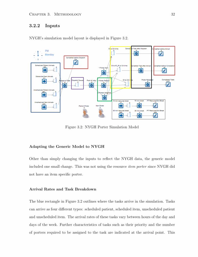
NYGH’s simulation model layout is displayed in Figure 3.2.
Figure 3.2: NYGH Porter Simulation Model
Adapting the Generic Model to NYGH
Other than simply changing the inputs to reflect the NYGH data, the generic model
included one small change. This was not using the resource item porter since NYGH did
not have an item specific porter.
Arrival Rates and Task Breakdown
The blue rectangle in Figure 3.2 outlines where the tasks arrive in the simulation. Tasks
can arrive as four different types: scheduled patient, scheduled item, unscheduled patient
and unscheduled item. The arrival rates of these tasks vary between hours of the day and
days of the week. Further characteristics of tasks such as their priority and the number
of porters required to be assigned to the task are indicated at the arrival point. This

Chapter 3. Methodology 33
breakdown of nine task types can be seen in Table 3.2. It is important to note that item
tasks never involve two porters and scheduled tasks always arrive as Routine, which is
why there is no breakdown based on number of porters involved in item transports and
no priority for scheduled tasks.
Table 3.2: Task Breakdown at NYGH
Task Type NYGH
Scheduled Patient 1 Porter 9.6%
Scheduled Patient 2 Porters 1.6%
Scheduled Item 4.6%
Unscheduled Patient STAT 1 Porter 16.6%
Unscheduled Patient STAT 2 Porters 4.5%
Unscheduled Patient Routine 1 Porter 30.3%
Unscheduled Patient Routine 2 Porters 11.0%
Unscheduled Item STAT 7.4%
Unscheduled Item Routine 14.4%
Dispatch Logic
After arriving and being classified into a task type, tasks will wait in the queue that is
surrounded by a purple border. For all tasks, there is a minimum wait time in the queue
of 30 seconds to account for the dispatcher to manually input the task information and
assign the task to a porter. The order in which tasks are assigned is based on priority
rules. The first rule states that STAT tasks will be given priority over Routine tasks.
The second rule states that a task can escalate in priority depending on how long it has
been waiting in the queue. STAT tasks are escalated almost instantly, scheduled tasks
will escalate in priority after 30 minutes and Routine tasks escalate after 60 minutes.

Chapter 3. Methodology 34
Resource Schedules and Breaks
The resources in the model are represented by the healthcare personnel at the bottom
of Figure 3.2 and are called upon at the activities surrounded by the green border to
process porter tasks. Their availability depends on the shift schedule that was obtained
by the portering manager. From there, the number of porters at work during any given
interval of 15 minutes was determined. Since NYGH does not have item specific porters,
only patient porters are used. The first activity surrounded by the green border requires
one porter to process a task and the second activity requires two porters.
In order to incorporate their breaks, a smaller simulation was built, in the bottom
right-hand corner of Figure 3.2. Whenever a porter’s break should be starting, a work
item will arrive in this smaller simulation and will require a resource to process it at
the activities. Requiring a resource at the break activities has a higher priority than the
activities where resources process porter tasks. This will ensure that resources start their
breaks on time. For example, if a porter becomes available and both a porter task and
a break work item are waiting to be processed, the porter will process the break work
item first. Porters assigned to a 4-hour shift receive one 15-minute break and porters
assigned to a 8-hour shift receive two 30-minute breaks. Porters often take a longer time
on break than allocated in their schedule. By analyzing daily porter transactions, it was
determined that instead of a 15-minute break, porters spend an average of 26 minutes
with a standard deviation of 10.56 minutes on break. For a 30-minute break, porters
spend an average of 36.54 minutes with a standard deviation of 9.89 minutes. Details of
the porter schedule can be seen in Appendix B.
Service Times
The part of the simulation where a resource spends time servicing a task is outlined
by the yellow border in Figure 3.2. This service time includes: personal response time

Chapter 3. Methodology 35
(dispatch to arrival) and task time (arrival to completion). Personal Response times
for different task types are considered and are modelled using a lognormal distribution
(including mean and standard deviation times as inputs) (Table 3.3). Task times are
only measured for three task types: patient 1 porter tasks, patient 2 porter tasks and
item 1 porter tasks (Table 3.4). Further breakdown by priority and whether the task
is scheduled or unscheduled is not necessary for task time because it was determined
that times were very similar between STAT, scheduled and 1 porter tasks for patient and
item tasks. Once this time has elapsed, tasks and resources move to the activities with
a black border in Figure 3.2. Here, the resource is released and available to be assigned
to another task.
Table 3.3: Personal Response Times at NYGH
Task Types AverageStandardDeviation
Scheduled Patient 1 Porter 4.63 6.98
Scheduled Patient 2 Porters 4.59 6.39
Scheduled Item 4.38 9.40
Unscheduled Patient STAT 1 Porter 4.10 5.37
Unscheduled Patient STAT 2 Porters 4.07 5.18
Unscheduled Patient Routine 1 Porter 4.73 7.58
Unscheduled Patient Routine 2 Porters 4.66 7.75
Unscheduled Item STAT 3.58 5.33
Unscheduled Item Routine 4.78 13.81
Table 3.4: Task Times at NYGH
Task Types AverageStandardDeviation
Patient 1 Porter 22.39 10.01
Patient 2 Porters 22.35 13.42
Item 1 Porter 13.51 10.63
Chapter 3. Methodology 36
Cancellation Rates and Time to Cancellation
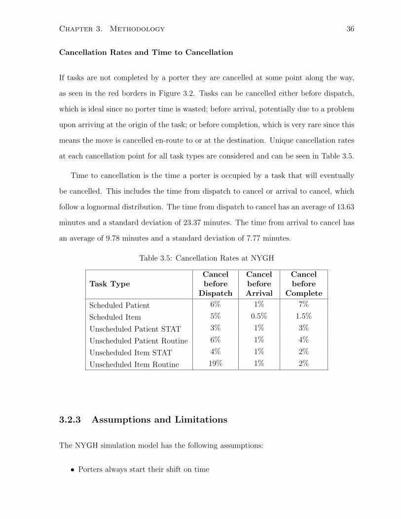
If tasks are not completed by a porter they are cancelled at some point along the way,
as seen in the red borders in Figure 3.2. Tasks can be cancelled either before dispatch,
which is ideal since no porter time is wasted; before arrival, potentially due to a problem
upon arriving at the origin of the task; or before completion, which is very rare since this
means the move is cancelled en-route to or at the destination. Unique cancellation rates
at each cancellation point for all task types are considered and can be seen in Table 3.5.
Time to cancellation is the time a porter is occupied by a task that will eventually
be cancelled. This includes the time from dispatch to cancel or arrival to cancel, which
follow a lognormal distribution. The time from dispatch to cancel has an average of 13.63
minutes and a standard deviation of 23.37 minutes. The time from arrival to cancel has
an average of 9.78 minutes and a standard deviation of 7.77 minutes.
Table 3.5: Cancellation Rates at NYGH
Task TypeCancelbefore
Dispatch
CancelbeforeArrival
Cancelbefore
Complete
Scheduled Patient 6% 1% 7%
Scheduled Item 5% 0.5% 1.5%
Unscheduled Patient STAT 3% 1% 3%
Unscheduled Patient Routine 6% 1% 4%
Unscheduled Item STAT 4% 1% 2%
Unscheduled Item Routine 19% 1% 2%
3.2.3 Assumptions and Limitations
The NYGH simulation model has the following assumptions:
• Porters always start their shift on time

Chapter 3. Methodology 37
• Porters will not start a new task 15 minutes before the end of their shift; the
simulation allows porters to finish tasks if they are already working on one
• Porters that only do linen tasks and porters that are off-system (do not receive
tasks through dispatching software) are not included in the number of available
resources in the simulation
• Scheduled tasks can be dispatched 30 minutes before their appointment time
• STAT tasks will be dispatched first, then Routine tasks
• All tasks will have a minimum wait time in the dispatch queue of 0.5 minutes to
account for the manual input of the task by the dispatcher
• Tasks escalate in priority based on task type and how long they have been waiting
for an available porter; STAT tasks are immediately escalated, scheduled tasks wait
30 minutes before escalating and Routine tasks wait 60 minutes before escalating
• Scheduled tasks have a priority of Routine
• Two porter tasks are known at receipt of the task; tasks cannot start as a one
porter task and then change to a two porter task
• Two porter tasks arrive in the simulation only between 7:00 and 17:00; there are
too few porters working outside these hours to handle a two porter task. If in
reality a two porter task exists outside these hours, a nurse or other staff member
will help with the task
Some aspects of the current situation at NYGH were not easily captured in the simulation
model. Those limitations are listed here:
• Normally for a two porter task, one porter becomes available first (primary porter)
and the second porter becomes available at a later time (secondary porter); to
simplify this concept in the simulation, the first porter will wait for the second to
become available and then both porters will be assigned to the task at the same
time
Chapter 3. Methodology 38
• The current simulation model does not take into account where a task originates or
its destination; this limits the simulation from using location as a basis of assigning
porters
• Due to the subjective judgment of the dispatchers at NYGH, the simulation model
will use a dispatching priority algorithm only based on how long a task has been
waiting in the queue and the original priority of the task
3.2.4 Validation
The simulation model was run using data from the current situation of portering at
NYGH. Key Performance Indicators of the current situation were compared with simula-
tion results. These KPIs are: percentage of scheduled tasks on-time (within 30 minutes),
percentage of tasks complete within 35 minutes of being received, dispatch time, trans-
port time and turnaround time. Figures 3.3 to 3.7 show results of KPIs during the
weekdays between 7AM and 5PM. In certain cases, the simulation matches the current
situation, however in other cases, the simulation does not match the current situation
exactly, reasons of which will be explained.
Figure 3.3 shows how long certain types of tasks will wait after being received to
being assigned to a porter, also known as the dispatch time. The simulation tends to
dispatch tasks 1-2 minutes faster than the current situation. This gap in performance is
partly due to the fact that sometimes a dispatcher will not dispatch a task even though
there is an available porter; the dispatcher is just waiting for an available porter close
to the origin of the next task. The simulation model does not have this logic built into
the dispatching algorithm and will therefore take less time to dispatch a task. Another
reason the simulation model dispatches tasks faster is that the model assumes there is a
30 second lag from receiving the task to dispatching the task, where in reality this time
could be longer depending how busy the dispatcher is at the time.

Chapter 3. Methodology 39
Figure 3.3: Validation of Dispatch Time
The differences between current situation transport times and simulation results are
very minimal, as seen in Figure 3.4. Sometimes the current situation has a faster trans-
port time and sometimes the simulation does, which is due to the variation in their
standard deviations.
Figure 3.4: Validation of Transport Time
Figure 3.5 shows that the turnaround time of the simulation is about two minutes
faster than the current situation. This graph is a combination of the previous two graphs;

Chapter 3. Methodology 40
adding dispatch time and transport time makes up turnaround time. Since the simulation
dispatch times were 1-2 minutes faster than the current situation and the transport times
were relatively even across the simulation and current situation, it makes sense that the
overall turnaround time has a similar difference between the simulation and current
compared to the dispatch times.
Figure 3.5: Validation of Turnaround Time
In Figure 3.6, the simulation completes 5-10% more tasks on time (within 30 minutes
of their appointment time) than does the current situation at NYGH. A reason the
current situation performs poorly compared to the simulation is that sometimes in reality
dispatchers forget about a scheduled task until a few minutes before its appointment time,
which makes it hard to complete the task within 30 minutes of the appointment. The
dispatching algorithm in the simulation will not forget about the scheduled tasks.
The percentage of tasks complete within 35 minutes is measured in Figure 3.7. This
35 minutes starts from the time a task is received to the time the porter completes the
task. The simulation completes around 10% more tasks than the current situation. The
reason for this is attributed to the difference in dispatch time between simulation and
current situation. Once assigned to a porter, tasks are not being completed any faster
by the simulation since their transport time is an input, therefore, the difference is due
to the dispatch time.

Chapter 3. Methodology 41
Figure 3.6: Validation of % Scheduled Tasks Completed by Appointment Time
Figure 3.7: Validation of % Unscheduled Tasks Completed within 35 minutes
These graphs were shared with hospital personnel at NYGH to ensure they were
satisfied with how the simulation represented the current situation. Since it was con-
cluded that the simulation developed accurately represents the current situation, results
of improvement scenarios will be compared to the base case simulation model, not to the
current situation at NYGH.

Chapter 3. Methodology 42
3.3 Simulation Model: JHCC
3.3.1 Data Analysis
After mapping out the porter process at JHCC, the appropriate data was requested.
JHCC has data collection software, Connexall, from which data from July 2013 to De-
cember 2013 was extracted. This data includes all porter tasks that took place in the
given time frame with details, similar to NYGH’s data, on each task. As with any ini-
tial raw data set, it came with inaccuracies. Delay reporting was not always completed
when a delay actually occurred, not all tasks completed by porters were recorded and
forgetfulness of porters to report on their progress all lead to inaccuracies in the data.
3.3.2 Inputs
JHCC’s simulation model layout is displayed in Figure 3.8.
Figure 3.8: JHCC Porter Simulation Model

Chapter 3. Methodology 43
Adapting the Generic Model to JHCC
The generic model did not need to go through any changes, other than changing the
input values to reflect the JHCC data, in order to be adapted to JHCC.
Arrival Rates and Task Breakdown
In JHCC’s simulation model, the blue border in Figure 3.8 indicates where tasks arrive.
Tasks can arrive in one of four ways: scheduled patient, scheduled item, unscheduled
patient and unscheduled item. Table 3.6 shows the breakdown of the nine task types at
JHCC. At their arrival, tasks are given a priority and the number of porters required,
based on the task breakdown. At JHCC, tasks are given an original priority level of 0
or 2-8, where levels 0 and 2 represent a higher priority task (STAT task) and levels 3-8
represent a lower priority task (Routine task). Even though tasks cannot originate as a
priority level 1, they can escalate from a level 2 to a level 1. The most common task
types of each priority are shown in Table 3.7.
Table 3.6: Task Breakdown at JHCC
Task Type JHCC
Scheduled Patient 1 Porter 11.43%
Scheduled Patient 2 Porters 0.31%
Scheduled Item 1.91%
Unscheduled Patient STAT 1 Porter 7.81%
Unscheduled Patient STAT 2 Porters 1.12%
Unscheduled Patient Routine 1 Porter 28.78%
Unscheduled Patient Routine 2 Porters 1.55%
Unscheduled Item STAT 0.04%
Unscheduled Item Routine 47.04%

Chapter 3. Methodology 44
Table 3.7: Priority Level Analysis
PriorityLevel
Most CommonTask Types
PercentageSecond Most
Common TaskTypes
Percentage
0 PACU 48% Emergency 25%2 Express Unit 30% Ambulatory Unit 11%3 Transfusion Medicine 21% X-Ray 11%4 Transfusion Medicine 10% Lab Core 10%5 Medicine Nurse 14% Surgical Nurse 11%6 Patient Registration 13% Scheduled Run 8%7 Scheduled Run 19% Endocrinology 8%8 Patient Registration 24% ICU Nurse 5%
Dispatch Logic
Surrounded by a purple border in Figure 3.8 is the dispatch queue. The task with the
highest priority when a porter is available will be dispatched. This priority is calculated
based on two rules. The first rule states that STAT tasks will be given priority over
Routine tasks. The second rule states that a task can escalate in priority depending on
how long it has been waiting in the queue. STAT tasks can originate as priority 0 or 2
and Routine tasks can originate as priority 3-8 with priorities 7 and 8 always being item
tasks, and priorities 3-6 primarily being patient tasks. STAT tasks escalate in priority
after waiting 14 minutes, scheduled tasks escalate after 22 minutes and Routine tasks
escalate after 30 minutes.
Resource Schedules and Breaks
Once a porter becomes available, s/he will be assigned to a task at points in the simulation
surrounded by a green border. JHCC has patient porters and item porters. Patient
porters can be assigned to both patient and item tasks, while item porters can only be
assigned to item tasks.
To incorporate porter breaks, a smaller simulation was built, in the bottom right-hand

Chapter 3. Methodology 45
corner of Figure 3.8. Porters assigned to a 4-hour shift receive one 15-minute break and
porters assigned to an 8-hour shift receive two 15-minute breaks and one 30-minute break.
Porters often take a longer time on break than allocated in their schedule. Instead of a
15-minute break, porters spend an average of 17.98 minutes with a standard deviation of
5.29 minutes on break. For a 30-minute break, porters spend an average of 32.80 minutes
with a standard deviation of 7.28 minutes. Details of the porter schedule can be seen in
Appendix B.
Service Times
Once the task has the correct number of resources assigned to it, it will move to the
points in the simulation surrounded by a yellow border in Figure 3.8 and the time each
task spends at each point with the assigned porter is known as the task’s service time.
This service time includes: arrival minutes (dispatch to in progress) and patient minutes
(in progress to completion). The arrival minutes for different task types are considered
and are modelled using a lognormal distribution (including mean and standard deviation
times as inputs) (Table 3.8). Patient minutes are only measured for three task types:
patient 1 porter tasks, patient 2 porter tasks and item 1 porter tasks (Table 3.9). Further
breakdown by priority and whether the task is scheduled or unscheduled is not necessary
for task time because it was determined that times were very similar between STAT,
scheduled and 1 porter tasks for patient and item tasks. Once this time has elapsed,
tasks and resources move to the next set of activities, outlined by the black border. The
resource is now released and available to be assigned to another task.

Chapter 3. Methodology 46
Table 3.8: Arrival Minutes at JHCC
Task Types AverageStandardDeviation
Scheduled Patient 1 Porter 21.18 8.60
Scheduled Patient 2 Porters 26.57 10.07
Scheduled Item 15.14 14.32
Unscheduled Patient STAT 1 Porter 18.47 10.21
Unscheduled Patient STAT 2 Porters 20.73 9.89
Unscheduled Patient Routine 1 Porter 17.87 12.69
Unscheduled Patient Routine 2 Porters 24.39 9.89
Unscheduled Item STAT 9.40 9.47
Unscheduled Item Routine 13.32 13.25
Table 3.9: Patient Minutes at JHCC
Task Types AverageStandardDeviation
Patient 1 Porter 7.80 8.38
Patient 2 Porters 7.74 7.76
Item 1 Porter 4.25 7.56
Cancellation Rates and Time to Cancellation
The simulation points that are outlined by a red border in Figure 3.8 identify the three
cancellation points: before dispatch, before task is in progress, and before completion.
Unique cancellation rates at each cancellation point for all task types are considered and
can be seen in Table 3.10. Time to cancellation is the time from dispatch to cancel or in
progress to cancel; these times follow a lognormal distribution. Time from dispatch to
cancel has an average of 15.41 minutes and standard deviation of 19.55 minutes. Time
from in progress to cancel has an average of 6.38 minutes and a standard deviation of
8.19 minutes.

Chapter 3. Methodology 47
Table 3.10: Cancellation Rates at JHCC
Task TypeCancelbefore
Dispatch
CancelbeforeArrival
Cancelbefore
Complete
Scheduled Patient 1.5% 8.8% 0.7%
Scheduled Item 0.2% 1.2% 0.2%
Unscheduled Patient STAT 1.7% 4.4% 0.2%
Unscheduled Patient Routine 2.2% 3.2% 0.1%
Unscheduled Item STAT 4.3% 9.1% 0%
Unscheduled Item Routine 1% 1.3% 0.1%
3.3.3 Assumptions and Limitations
The simulation model has the following assumptions:
• Porters always start their shift on time
• Porters will not start a new task 15 minutes before the end of their shift; simulation
allows porters to finish tasks if they are already working on one
• Porters that only do linen tasks and porters that are off-system (do not receive
tasks through dispatching software) are not included in the number of available
resources of the simulation
• Item porters are included as a separate resource and can only complete item tasks
• Patient porters complete both item tasks and patient tasks
• Scheduled tasks can be dispatched 30 minutes before their appointment time
• STAT tasks include tasks with a priority of 0, 1 or 2 and Routine tasks have a
priority of 3-8
• All tasks are dispatched first come first served within priority class
• All tasks will have a minimum wait time in the dispatch queue of 0.1 minutes to
account for a lag in the dispatching software

Chapter 3. Methodology 48
• Tasks escalate in priority based on task type and how long they have been waiting
for an available porter; STAT tasks wait 14 minutes before escalating, scheduled
tasks wait 22 minutes before escalating, Routine tasks wait 30 minutes before es-
calating
• Two porter tasks are known at receipt of the task; tasks cannot start as a one
porter task and then change to a two porter task
• Two porter tasks arrive in the simulation only between 7:00 and 20:00; there are
too few porters working outside these hours to handle a two porter task. If in
reality a two porter task exists outside these hours, a nurse or other staff member
will help with the task
Some aspects of the current situation were not easily captured in the simulation model.
Those limitations are listed here:
• Normally for a two porter task, one porter becomes available first (primary porter)
and the second porter becomes available at a later time (secondary porter); to
simplify this concept in the simulation, the first porter will wait for the second to
become available and then both porters will be assigned at the same time
• The current simulation model does not take into account where a task originates or
its destination; this limits the simulation from using location as a basis of assigning
porters
• The automated dispatch system at JHCC described in section 1.1.2 is highly com-
plex including multiple priority levels; the dispatching algorithm in the simulation
model only uses two priority levels
3.3.4 Validation
Key Performance Indicators defined by JHCC were used to validate the simulation model
against the current porter situation. These KPIs are: percentage of prebooked tasks

Chapter 3. Methodology 49
on time (within 15 minutes), percentage of tasks complete within 30 minutes of being
received, dispatch time, trip time and transaction time. Figures 3.9 to 3.12 show KPI
results for weekdays between the hours of 7AM and 5PM and the graphs show that in
certain cases, the simulation matches the current situation very well, however in other
cases, the simulation may not match the current situation, the reasons for which will be
explained.
Figure 3.9 shows the time a task spends waiting for an available porter during the
weekdays and between 7AM-5PM. Tasks will spend more time, around one minute longer,
waiting for an available porter in the simulation compared to the current situation.
Figure 3.9: Validation of Dispatch Time
Figure 3.10 shows the trip time of the current situation and the simulation model
results. The current situation almost always matches the simulation. This makes sense
since trip time is an input. Sometimes the current situation has a faster trip time and
sometimes the simulation does, which is due to the variation in their standard deviations.
Figure 3.11 shows the transaction time comparison between the current situation and
the simulation result. Tasks in the simulation take about one minute longer on average
than the current situation. This transaction time combines dispatch time and trip time.
Since the simulation dispatch times were one minute slower than the current situation and

Chapter 3. Methodology 50
Figure 3.10: Validation of Trip Time
the trip times were relatively even across the simulation and current situation, it makes
sense that the overall transaction time has a similar difference between the simulation
and current to these dispatch times.
Figure 3.11: Validation of Transaction Time
In Figure 3.12, it is seen that there is minimal difference between the % prebooked
tasks completed on time resulting from the simulation and the current performance at
JHCC. The only task type where there is a significant difference between current and

Chapter 3. Methodology 51
simulation is the scheduled 2 porter tasks. By looking at the graph, the simulation
completes about 15% less tasks on time compared to the current situation. This is
because in the current situation, 2 porter tasks are always assigned as STAT, whereas in
the simulation, all scheduled tasks, both 1 and 2 porter tasks, have a priority of Routine.
Therefore, it will take longer for a scheduled 2 porter task to be escalated in priority in
the simulation and therefore, less likely to be completed on time.
Figure 3.12: Validation of % Prebooked Tasks On Time
The percentage of tasks complete within 30 minutes is measured in Figure 3.13. This
30 minutes includes the time from when a task is received to the time the porter completes
that task. The results vary between the current situation completing more tasks within
the target time and the simulation completing more tasks.
These graphs and other results of comparing the current situation with the simulation
performance were shared with hospital personnel at JHCC to ensure they were satisfied
with how the simulation represented the current situation. Since it was concluded that the
simulation developed accurately represents the current situation, results of improvement
scenarios will be compared to the base case simulation model, not to the current situation
at JHCC.

Chapter 3. Methodology 52
Figure 3.13: Validation of % Tasks Completed within 30 minutes

Chapter 4
Scenario Testing
The scenarios described in the following sections were developed in collaboration with
the hospitals.
4.1 Improvement Scenarios: NYGH
Scenario 1: Adding Weekday Shifts
This improvement scenario simulates how porter performance metrics are affected if a
new porter were hired during a weekday shift. Additions of 8-hour and 4-hour shifts
are simulated. The times of these additional shifts were determined by looking at the
demand of porter tasks entering the system at each hour of the day and comparing if the
supply of porters working during each hour was able to meet this demand. A supply-
demand graph shows these differences for an average Thursday (Figure 4.1). The times
throughout the day where demand most exceeds supply are where additional porter shifts
are added. These shifts are identified in Table 4.1.
53

Chapter 4. Scenario Testing 54
Figure 4.1: Supply-Demand Graph for an Average Thursday
Table 4.1: Adding Weekday Shifts
Scenario Details Shift Time Break Times
1AAdd an 8-hour
shift8:00-16:00 10:30-11:00/ 14:00-14:30
1BAdd a 4-hour
shift10:30-14:30 12:00-12:15
1CAdd two 8-hour
shifts8:00-16:00 and
10:00-18:00
10:30-11:00/ 14:00-14:30and 11:30-12:00/
15:30-16:00
1DAdd two 4-hour
shifts10:30-14:30 and
13:30-17:3012:00-12:15 and 15:15-15:30
1EAdd an 8-hour
and 4-hour shift8:00-16:00 and
10:30-14:3010:30-11:00/ 14:00-14:30
and 12:00-12:15
Scenario 2: Adding Weekend Shifts
This improvement scenario simulates how porter performance metrics are affected if a
new porter were hired during a weekend shift. Additions of 8-hour and 4-hour shifts are
simulated. The times of these additional shifts were determined using a similar method
to Scenario 1 (Figure 4.2) and can be seen in Table 4.2.

Chapter 4. Scenario Testing 55
Figure 4.2: Supply-Demand Graph for an Average Saturday
Table 4.2: Adding Weekend Shifts
Scenario Details Shift Time Break Times
2AAdd an 8-hour
shift8:00-16:00 10:30-11:00/ 13:30-14:00
2BAdd a 4-hour
shift9:00-13:00 11:30-11:45
2CAdd an 8-hour
and 4-hour shift8:00-16:00 and
9:00-13:0010:30-11:00/ 13:30-14:00
and 11:30-11:45
Scenario 3: Altering Weekday and Weekend Schedules
This improvement scenario simulates how porter performance metrics would be affected if
current porter shifts were altered to better meet demand. To do this, the following metrics
were used to assess the base case scenario’s performance by hour of day: % Scheduled
tasks on time, % STAT and Routine Tasks completed within 35 minutes, Dispatch time
of STAT and Routine tasks and Turnaround time of all unscheduled tasks. The averages
for each of these metrics were determined between the hours of 7:00 and 20:00. Then,
it was determined which hours performed below these averages. The hours that were
below average forthe % completed on time, shown in Figures 4.3 and 4.4, were consistent
across all metrics. These hours are between 11:00-13:00 and 17:00-19:00 on the weekdays
and 10:00-12:00 and 16:00-18:00 on the weekends. Since these time frames are around

Chapter 4. Scenario Testing 56
lunch or dinner, the poor performance is due to too many porters assigned a break at
this time. Based on these hours, current schedules were shifted to add porters to these
poor performing hours. The changes resulting from this analysis can be seen in Tables
4.3 and 4.4.
Figure 4.3: Determining Poor Performing Weekday Hours
Figure 4.4: Determining Poor Performing Weekend Hours
Scenario 4: Improving Personal Response Time
This improvement scenario simulates how porter performance metrics would be affected
if personal response time was reduced. This reduction of personal response time is used

Chapter 4. Scenario Testing 57
Table 4.3: Changing Weekday Shifts
ScenarioOldShift
OldBreak 1
OldBreak 2
NewShift
NewBreak 1
NewBreak 2
3A12:00-16:00
14:00-14:15
10:00-14:00
12:00-12:15
3B13:00-17:00
15:00-15:15
17:00-21:00
19:00-19:15
Table 4.4: Changing Weekend Shifts
ScenarioOldShift
OldBreak 1
OldBreak 2
NewShift
NewBreak 1
NewBreak 2
3C12:00-20:00
14:30-15:00
18:00-18:30
11:00-19:00
13:30-14:00
16:30-17:00
3D11:00-15:00
13:00-13:15
10:00-14:00
11:45-12:00
to simulate the use of iPads or other tablet devices which have the potential to speed
up the dispatch process. Using these devices would enable the porters to report on
their progress without having to spend time searching for a landline. This scenario also
simulates if reducing elevator delays and time searching for equipment has the potential
to improve porter performance.
The personal response time is represented using a lognormal distribution. Currently,
NYGH has an average personal response time of 4.48 minutes. For this scenario, this
time was reduced by 1, 2 and 3 minutes and the scenarios were labelled scenario 4A, 4B,
and 4C, respectively. The standard deviation of the base case personal response time was
reduced proportionally to match the lognormal distribution of the base case scenario.
Scenario 5: Improving Task Time
This improvement scenario simulates how porter performance metrics would be affected if
task time was reduced. This reduction of task time is used to simulate how improvements
in patient readiness, elevator delays and other delays would affect porter performance.
Chapter 4. Scenario Testing 58
The current average task time at NYGH is 20.12 minutes. Similarly to Scenario 4, this
time was reduced by 1, 2 and 3 minutes to represent scenarios 5A, 5B, and 5C.
Scenario 6: Reclassifying Two Porter Tasks
This improvement scenario simulates how porter performance metrics would be affected if
50% of two porter tasks were reclassified. This reduction is used to simulate if the hospital
purchased new equipment where two porters are no longer needed. This scenario also
simulates if room to room transfers only required one porter rather than two. In the base
case scenario, 19% of tasks involve two porters. This number will be reduced to 9.5% in
this scenario and the number of one porter tasks will increase to 90.5%.
Scenario 7: Reclassifying STAT Tasks
This improvement scenario simulates how porter performance metrics are affected if 50%
of STAT tasks were reclassified. This reduction is used to simulate the use of better
classification and usage of a STAT task by hospital departments. Currently, over 90%
of tasks originating at or destined to Angiography, Endocrinology and the Operating
Room are classified as STAT. Tasks in these departments may not be theoretical STAT
tasks, but are classified as STAT because these departments know that the task will get
completed faster that way. In the base case scenario, 34% of tasks are STAT tasks. This
number will be reduced to 17% in this scenario and the number of Routine tasks will
increase to 83%.
Scenario 8: Combining other improvement scenarios
Scenario 8 makes up seven scenarios where previously mentioned improvements will be
combined to achieve results closer NYGH’s targets (Table 4.5).

Chapter 4. Scenario Testing 59
Table 4.5: Scenario 8 Improvements
ScenarioScenariosCombined
Weekday/WeekendAffected
8A 3A, 3B, 4C, 5A & 6 Weekday
8B 3C, 3D, 4C, 5A & 6 Weekend
8C 3A, 3B & 4C Weekday
8D 3C, 3D & 4C Weekend
8E 4C & 5A Both
8F 4C & 6 Both
8G 4C, 5A & 6 Both
4.2 Improvement Scenarios: JHCC
Scenario 1: Adding Weekday Shifts
This improvement scenario simulates how porter performance metrics are affected if a
new porter is hired during a weekday shift. Additions of 8-hour and 4-hour shifts are
simulated. The times of these additional shifts were determined by matching supply
and demand. A supply-demand graph shows these differences for an average Thursday
(Figure 4.5). The times throughout the day where demand most exceeds supply are
where additional porter shifts are added. These shifts are identified in Table 4.6.
Figure 4.5: Supply-Demand Graph for an Average Thursday

Chapter 4. Scenario Testing 60
Table 4.6: Adding Weekday Shifts
Scenario Details Shift Time Break Times
1AAdd an 8-hour
shift7:00-15:00
9:00-9:15 / 11:15-11:45 /13:45-14:00
1BAdd two 8-hour
shifts7:00-15:00 and
7:30-15:30
9:00-9:15 / 11:15-11:45 /13:45-14:00 and 9:30-9:45 /11:45-12:15 / 14:15-14:30
1CAdd a 4-hour
shift7:00-11:00 9:00-9:15
1DAdd two 4-hour
shifts7:00-11:00 and
12:00-16:009:00-9:15 and 14:00-14:15
1EAdd an 8-hour
and 4-hour shift7:00-15:00 and
7:00-11:009:00-9:15 / 11:15-11:45 /13:45-14:00 and 9:00-9:15
Scenario 2: Adding Weekend Shifts
This improvement scenario simulates how porter performance metrics are affected if a
new porter were hired during a weekend shift. Additions of both 8-hour and 4-hour
shifts are simulated. The times of these additional shifts were determined using a similar
method to Scenario 1 (Figure 4.6) and can be seen in Table 4.7.
Figure 4.6: Supply-Demand Graph for an Average Saturday

Chapter 4. Scenario Testing 61
Table 4.7: Adding Weekend Shifts
Scenario Details Shift Time Break Times
2AAdd an 8-hour
shift7:00-15:00
9:00-9:15 / 11:30-12:00 /13:45-14:00
2BAdd a 4-hour
shift10:00-14:00 12:00-12:15
2CAdd an 8-hour
and 4-hour shift7:00-15:00 and
10:00-14:009:00-9:15 / 11:30-12:00 /
13:45-14:00 and 12:00-12:15
Scenario 3: Altering Weekday and Weekend Schedules
This improvement scenario simulates how porter performance metrics would be affected
if current porter shifts were altered to better meet demand. To do this, the following
metrics were used to assess the base case scenario’s performance by hour of day: %
Prebooked tasks on time, % STAT and Routine tasks completed within 40 minutes,
Dispatch time of STAT and Routine tasks and Transaction time of all demand tasks.
The averages for each of these metrics were determined between the hours of 7:00 and
20:00. Then, it was determined which hours performed below these averages. The hours
that were below average forthe % completed within 40 minutes, shown in Figures 4.7
and 4.8, were consistent across all metrics. These hours are between 7:00-17:00 on the
weekdays and 8:00-16:00 on the weekends. Based on these hours, current schedules were
shifted to add porters to these poorly performing hours. The new shift and break times
resulting from this analysis can be seen in Tables 4.8 and 4.9.
Table 4.8: Changing Weekday Shifts
ScenarioOldShift
OldBreak
1
OldBreak
2
OldBreak
3
NewShift
NewBreak
1
NewBreak
2
NewBreak
3
3A15:00-19:00
17:00-17:15
7:00-11:00
9:00-9:15
3B16:00-00:00
17:30-17:45
20:00-20:30
21:45-22:00
7:30-15:30
9:15-9:30
11:30-12:00
14:00-14:15

Chapter 4. Scenario Testing 62
Table 4.9: Changing Weekend Shifts
ScenarioOldShift
OldBreak
1
OldBreak
2
OldBreak
3
NewShift
NewBreak
1
NewBreak
2
NewBreak
3
3C15:00-23:00
17:15-17:30
18:30-19:00
21:30-21:45
8:00-16:00
10:15-10:30
11:30-12:00
14:00-14:15
3D12:00-20:00
14:45-15:00
17:15-17:45
18:30-18:45
10:00-18:00
12:45-13:00
15:15-15:45
16:30-16:45
Figure 4.7: Determining Poor Performing Weekday Hours
Figure 4.8: Determining Poor Performing Weekend Hours
Scenario 4: Improving Arrival Minutes
This improvement scenario simulates how porter performance metrics would be affected
if arrival minutes were reduced. Arrival minutes include the time from dispatch to in

Chapter 4. Scenario Testing 63
progress. This reduction of arrival minutes is used to simulate how improvements in
patient readiness, elevator delays and time searching for equipment would affect porter
performance.
To adjust the base case to model this scenario, the average of the base case arrival
minutes (16.14 minutes) was reduced by 1, 2 and 3 minutes and the scenarios were
labelled scenario 4A, 4B, and 4C, respectively. The standard deviation of the base case
arrival minutes was reduced proportionally to match the lognormal distribution of the
base case scenario.
Scenario 5: Improving Patient Minutes
This improvement scenario simulates how porter performance metrics would be affected
if patient minutes were reduced. This reduction of patient minutes is used to simulate
if upper floors were used to transport patients rather than going down to the basement.
The current average patient minutes at JHCC is 6.05 minutes. Similarly to Scenario 4,
this time was reduced by 1, 2 and 3 minutes to represent scenarios 5A, 5B, and 5C.
Scenario 6: Combining other improvement scenarios
Scenario 6 makes up three scenarios where previously mentioned improvements will be
combined to achieve results closer JHCC’s targets (Table 4.10).
Table 4.10: Scenario 6 Improvements
ScenarioScenariosCombined
Weekday/WeekendAffected
6A 3A, 3B & 4C Weekday
6B 3C, 3D & 4C Weekend
6C 4C & 5A Both

Chapter 4. Scenario Testing 64
4.3 Sensitivity Analysis: NYGH
The scenarios described in Table 4.11 are tested using the simulation model to determine
how the current porter system could handle increases in personal response time, in task
time, in demand of certain task types, or even in demand overall. To adjust the base
case to each of the scenarios here, similar methods in the Improvement Scenarios section
of this report were used. Scenario 9 involves increasing and decreasing overall demand.
To do this, demand rates for each day of the week were calculated and they were either
increased or decreased by 10%. The difference in demand between the base case and
either this increase or decrease was calculated. The increased demand was added across
various hours between 7:00 and 23:00 and the decreased demand was removed from
various hours between 7:00 and 23:00.
Table 4.11: Sensitivity Analysis Scenarios: NYGH
Scenario FactorIncrease orDecrease
Amount
4DPersonal Response
TimeIncrease 1 minute
5D Task Time Increase 1 minute6B # Two porter tasks Increase 50%7B # STAT Tasks Increase 50%9A Demand Increase 10%9B Demand Decrease 10%

Chapter 4. Scenario Testing 65
4.4 Sensitivity Analysis: JHCC
Sensitivity testing was also done on the JHCC simulation model. These include increasing
arrival minutes, patient minutes, increasing demand and decreasing demand. These
scenarios are described in Table 4.12.
Table 4.12: Sensitivity Analysis Scenarios: JHCC
Scenario FactorIncrease orDecrease
Amount
4D Arrival Minutes Increase 1 minute5D Patient Minutes Increase 1 minute7A Demand Increase 10%7B Demand Decrease 10%

Chapter 5
Results
This chapter describes the results of scenario testing at the two hospitals involved in this
research: North York General Hospital and Juravinski Hospital and Cancer Center.
5.1 Simulation Results: NYGH
Once the generic simulation model included all the NYGH inputs from historical data and
this simulation was validated according to the current performance at NYGH, scenario
testing began. Table 5.1 summarizes NYGH’s scenarios. The simulation model was run
10 times for each scenario tested to account for variation in arrival rates, service times,
cancellation rates and break times. The simulation was also run for 10 trials because this
was an appropriate sample size to calculate a 90% confidence interval. This confidence
interval was calculated to ensure that 90% of the time, the mean is within a certain
range (see Table 5.2 for these ranges). Confidence intervals for weekend results can be
seen in Appendix C. In order to reduce these intervals, more trials are required. Results
by hour for an average weekday and weekend were collected for all five KPIs and for
many different task types. In this report, the results of the following task types for the
66

Chapter 5. Results 67
five KPIs will be discussed (Table 5.3).
Table 5.1: NYGH Scenario Legend
Scenario Description1A Adding one weekday 8-hour shift1B Adding two weekday 8-hour shifts1C Adding one weekday 4-hour shift1D Adding two weekday 4-hour shifts1E Adding one weekday 8-hour and one 4-hour shift2A Adding one weekend 8-hour shift2B Adding one weekend 4-hour shift2C Adding one weekend 8-hour and one 4-hour shift3A Change weekday 4-hour morning shift3B Change weekday 4-hour afternoon shift3C Change weekend 8-hour afternoon shift3D Change weekend 4-hour afternoon shift4A Reduce Personal Response time by 1 minute4B Reduce Personal Response time by 2 minutes4C Reduce Personal Response time by 3 minutes4D Increase Personal Response time by 1 minute5A Reduce Task time by 1 minute5B Reduce Task time by 2 minutes5C Reduce Task time by 3 minutes5D Increase Task time by 1 minute6 Reclassify 50% of two porter tasks
6B Increase # two porter tasks by 50%7 Reclassify 50% of STAT tasks
7B Increase # STAT tasks by 50%8A Combination of 3A, 3B, 4C, 5A & 68B Combination of 3C, 3D, 4C, 5A & 68C Combination of 3A, 3B & 4C8D Combination of 3C, 3D & 4C8E Combination of 4C& 5A8F Combination of 4C & 68G Combination of 4C, 5A & 69A Increase Demand by 10%9B Decrease Demand by 10%
Results in Figures 5.1 and 5.2 display the turnaround times of all scenarios tested
compared to the base case during the weekday and weekend (refer to Appendix C for
the details). These figures show that all scenarios tested improve on the base case result.

Chapter 5. Results 68
Table 5.2: NYGH Confidence Intervals for Weekday Results
Scenario Mean90% Confidence
IntervalBase Case 39.57 1.08
1A 34.47 0.931B 33.64 1.721C 37.90 1.741D 37.19 1.921E 32.02 1.573A 37.61 1.883B 38.49 1.764A 36.25 1.124B 35.37 1.494C 32.40 1.655A 38.19 0.915B 37.86 1.155C 34.25 2.096 35.19 1.617 38.47 1.55
8A 23.38 1.228C 32.20 2.368E 27.16 1.298F 26.17 0.558G 24.34 1.04
This means that implementing any of the suggested scenarios will result in an improved
turnaround time, and several of the scenarios even result in a turnaround time that
achieves the target of 35 minutes. Again, refer to Table 5.2 for ranges of these results.
From Figure 5.1, it is seen that Scenarios 8A, 8C, 8E, 8F and 8G meet the target
turnaround time of 35 minutes and also have a shorter turnaround time than adding a
full time and part time porter. Often times, adding a resource is seen as an easy solution,
but this analysis shows that there exist other alternatives to this. Similar results can be
seen for the weekend (Figure 5.2).
Figures 5.3 and 5.4 show results of sensitivity analysis by comparing average turnaround
times of each scenario. The gap between performance and target is increasing for the

Chapter 5. Results 69
Table 5.3: KPIs resulting from Simulation
KPI Task Type% Scheduled tasks on-time Scheduled% Tasks complete within 35 minutes of receipt STAT, RoutineDispatch time STAT, RoutineTransport time Scheduled, STAT, RoutineTurnaround time Unscheduled
Figure 5.1: Weekday Turnaround Time: Evaluating Improvement Scenarios
scenarios tested here.
In summary, the results show that during the weekday, Scenario 8A performs the best
and during the weekend, Scenario 8B performs the best. This is because these scenarios
combine multiple improvement scenarios together to ensure that the target turnaround
time of 35 minutes is achieved. The combined improvements include reducing personal
response time, reducing task time, reclassifying two porter tasks, and altering existing
schedules. By implementing these scenarios, a weekday turnaround time of 23.38 minutes
and weekend turnaround time of 29.96 minutes will result.
To reduce personal response time by three minutes (Scenario 4C), NYGH will need to
implement projects or gain support from management to eliminate pager use by switching

Chapter 5. Results 70
Figure 5.2: Weekend Turnaround Time: Evaluating Improvement Scenarios
Figure 5.3: Weekday Turnaround Time: Sensitivity Analysis
Figure 5.4: Weekend Turnaround Time: Sensitivity Analysis
to a tablet or smart phone system, revise policy on targets for personal response times,
and pre-assign porters for the next job prior to completing the current task.

Chapter 5. Results 71
To reduce task time by one minute (Scenario 5A), NYGH will need to: change policies
in order to reduce unit, patient or elevator delays, better manage the productivity of
porters, and improve access to equipment.
To reclassify the number of two porter tasks (Scenario 6), unit staff at NYGH will
need to be utilized more for room to room transfers, or the policy on when two porters
are needed for a transport will need to be revised.
Finally, in order to alter existing schedules both during the weekdays (Scenario 3A
& 3B) and weekends (Scenario 3C & 3D), discussions must be had with the Union to
determine if changes to the collective agreement need to be made.

Chapter 5. Results 72
5.2 Simulation Results: JHCC
The JHCC simulation model was also run 10 times for each scenario tested to account for
variation in arrival rates, service times, cancellation rates and break times. Similarly to
NYGH, the simulation was also run for 10 trials because this was an appropriate sample
size to calculate a 90% confidence interval. This confidence interval was calculated to
ensure that 90% of the time, the mean is within a certain range (see Table 5.5 for these
ranges). Confidence intervals for weekend results can be seen in Appendix C. Table 5.4
summarizes JHCC’s scenarios. Results by hour for an average weekday or weekend were
collected for all six KPIs and for many different task types. In this report, the results of
the following task types for the five KPIs will be discussed (Table 5.6).
Results in Figures 5.5 and 5.6 display the turnaround times of all scenarios tested
compared to the base case during the weekday and weekend (refer to Appendix C for
the details). These figures show that all scenarios tested improve on the base case result.
This means that implementing any of the suggested scenarios will result in an improved
turnaround time, and several of the scenarios even result in a turnaround time that
achieves the target of 30 minutes. Again, refer to Table 5.5 for ranges of these results.
Figure 5.5 shows that Scenarios 4C, 5B, 5C, 6A and 6C meet the target turnaround
time of 30 minutes and also have a shorter turnaround time than adding a full time and
part time porter. JHCC was very excited about this result and they were glad to have
this evidence to support a future decision regarding staffing. Similar results can be seen
for the weekend (Figure 5.6).
Figures 5.7 and 5.8 show results of sensitivity analysis by comparing average turnaround
times of each scenario. The gap between performance and target is increasing for the
scenarios tested here.
In summary, the results show that during the weekday, Scenario 6A performs the best

Chapter 5. Results 73
Table 5.4: JHCC Scenario Legend
Scenario Description1A Adding one weekday 8-hour shift1B Adding two weekday 8-hour shifts1C Adding one weekday 4-hour shift1D Adding two weekday 4-hour shifts1E Adding one weekday 8-hour and one 4-hour shift2A Adding one weekend 8-hour shift2B Adding one weekend 4-hour shift2C Adding one weekend 8-hour and one 4-hour shift3A Change weekday 4-hour morning shift3B Change weekday 8-hour morning shift3C Change weekend 8-hour afternoon shift3D Change weekend 8-hour afternoon shift4A Reduce Arrival minutes by 1 minute4B Reduce Arrival minutes by 2 minutes4C Reduce Arrival minutes by 3 minutes4D Increase Arrival minutes by 1 minute5A Reduce Patient minutes by 1 minute5B Reduce Patient minutes by 2 minutes5C Reduce Patient minutes by 3 minutes5D Increase Patient minutes by 1 minute6A Combination of 3A, 3B & 4C6B Combination of 3C, 3D & 4C6C Combination of 4C& 5A7A Increase Demand by 10%7B Decrease Demand by 10%
and during the weekend, Scenario 6B performs the best. This is because these scenarios
combine multiple improvement scenarios together to ensure that the target turnaround
time of 30 minutes is achieved. The combined improvements include reducing arrival
minutes, reducing patient minutes and altering existing schedules. By implementing
these scenarios, a weekday transaction time of 24.21 minutes and weekend transaction
time of 21.08 minutes will result.
In order to reduce arrival minutes by three minutes (Scenario 4C), JHCC will need to
implement projects to reduce patient readiness delays, reduce time searching for equip-
ment and reduce elevator delays.

Chapter 5. Results 74
Table 5.5: JHCC Confidence Intervals for Weekday Results
Scenario Mean90% Confidence
IntervalBase Case 43.52 1.38
1A 35.12 3.121B 29.84 0.601C 37.51 2.491D 37.33 1.171E 33.59 1.253A 36.80 2.093B 35.72 1.004A 35.79 1.534B 34.07 2.244C 29.74 1.625A 36.30 1.465B 31.85 0.995C 27.70 0.916A 24.21 0.696C 25.91 1.26
Table 5.6: KPIs resulting from Simulation
KPI Task Type% Prebooked jobs on-time Scheduled% Tasks complete within 30 minutes of receipt STAT, RoutineDispatch time STAT, RoutineTrip minutes Scheduled, STAT, RoutineTransaction time UnscheduledBottlenecks All jobs
To reduce patient minutes by one minute (Scenario 5A), JHCC will investigate uti-
lizing upper floors to transport patients rather than always using the basement.
Finally, to alter existing schedules both during the weekdays (Scenario 3A & 3B) and
weekends (Scenario 3C & 3D), discussions must be had with the Union to determine if
changes to the collective agreement can be made.
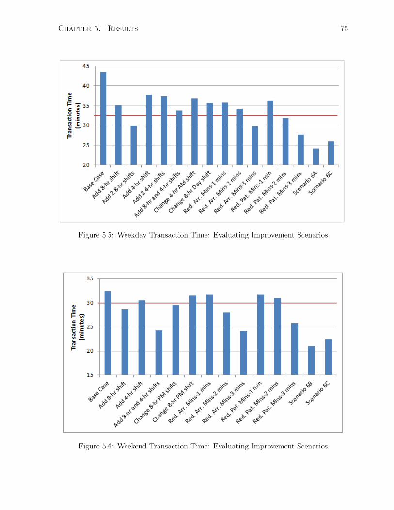
Chapter 5. Results 75
Figure 5.5: Weekday Transaction Time: Evaluating Improvement Scenarios
Figure 5.6: Weekend Transaction Time: Evaluating Improvement Scenarios

Chapter 5. Results 76
Figure 5.7: Weekday Transaction Time: Sensitivity Analysis
Figure 5.8: Weekend Transaction Time: Sensitivity Analysis

Chapter 6
Conclusion
The purpose of the research presented in this thesis was to model the patient transporta-
tion, or portering, department by developing a generic discrete event simulation. To
test its applicability, this model was used to represent the current porter operations at
two Toronto area hospitals: North York General Hospital and Juravinski Hospital and
Cancer Center. The simulation model was used to test improvement scenarios virtually
to see their impact on key performance metrics.
Once the simulation model was developed, it needed to be validated to ensure it
accurately represented the current situation at both hospitals involved in this research.
To validate the model, the current situation at the hospitals and the simulation result
were compared using KPIs such as % scheduled tasks completed on time, % unscheduled
tasks completed within the target turnaround time, dispatch time, transport time and
turnaround time. Historical data was analyzed to determine these KPIs for the current
situation, and simulation outputs were analyzed to determine KPIs for the simulation
result. Once their results were similar enough and hospital clients were happy with the
accuracy of the simulation, the research could move forward with scenario testing.
Scenarios were developed by the research team with heavy input from the hospitals.
77

Chapter 6. Conclusion 78
These scenarios were used to simulate improvements to the current process and how
these improvements would impact KPIs. Some scenarios included adding porters during
peak hours during with weekday and weekend, altering existing porter shifts, reducing
services times, and many combinations of multiple improvement scenarios in order to
reach the defined targets. It was determined that, for both hospitals, combining multiple
improvement scenarios together would produce the best result and many of the defined
targets for the key performance indicators would be met by implementing these improve-
ments. For example, at NYGH, if Scenario 8A was implemented, which involves changing
existing shifts, improving personal response time, improving task time and reclassifying
the number of two porter tasks, it would result in an average turnaround time of 23.38
minutes, an improvement from the base case turnaround time of 39.31 minutes. Similar
results were seen during the weekends (scenario 8B). Since these scenarios resulted in
the best turnaround time, it was recommended that NYGH implement scenario 8A to
see improvements during the weekdays and scenario 8B to see improvements during the
weekends. At JHCC, if Scenario 6A was implemented, which involves changing exist-
ing shifts, improving arrival minutes and improving patient minutes, an improvement of
13.65 minutes is realized, bringing the average turnaround time to 24.21 minutes dur-
ing the weekdays. Similar results were seen during the weekends (scenario 6B). Since
these scenarios resulted in the best turnaround time, it was recommended that JHCC
implement scenario 6A to see improvements during the weekdays and scenario 6B to see
improvements during the weekends.
This simulation model acted as a decision support tool for the hospitals involved to
move forward in their decision making process as to which improvement scenarios will
have the biggest impact on KPIs. The results were shared with NYGH and JHCC and
each hospital seemed enthusiastic about the improvements to portering that lie ahead.

Chapter 7
Future Research
To test the generality of the simulation model, for future research, it should be applied
to portering departments of at least three other hospitals. One hospital that has already
expressed interest in applying this model to improve their portering department is The
Scarborough Hospital, in Toronto. TSH has two hospital sites interested in using the
model. This will test the model’s applicability and there may be additions to the model
based on other hospital’s porter processes.
One of these additions could be including location as a further level of detail of each
task as this could increase the accuracy of the model. Currently at both hospitals studied
in this research, the dispatcher or manual dispatching system uses the starting location
of the task and the current location of an available porter to help assign porters to tasks
based on location proximity. This is done so that porters do not have to travel far empty
handed from finishing one task to starting the next. This aspect of the current situation
was found to be too difficult to capture in the current simulation model. To include this
in a new simulation model would require assigning a starting and ending location for
each task and ensuring the closest porter available is assigned.
Other areas of future research include finding ways to reduce the number of limitations
79

Chapter 7. Future Research 80
in the current model. For example, one option is changing a one porter task to a two
porter task after the first porter arrives at the origin. Another limitation to overcome
is including more logic in the dispatching system so that it can better reflect what a
human dispatcher’s decision making process involves. Overcoming these limitations and
applying the model to other hospitals to test its generality will increase the model’s
accuracy, and hence increase the confidence of its users.

Bibliography
[1] S. Landry and M. Beaulieu, “The Challenges of Hospital Supply Chain Management,
from Central Stores to Nursing Units,” in Handbook of Healthcare Operations Man-
agement: Methods and Applications (B. T. Denton, ed.), pp. 465–481, New York,
NY: Springer Science and business mediafbrin, 2013.
[2] J. Aherne and J. Whelton, Applying Lean in Healthcare: A Collection of Interna-
tional Case Studies. New York, NY: CRC Press, 2010.
[3] Health Canada, “About Health Canada.” http://www.hc-sc.gc.ca/ahc-asc/
activit/about-apropos/index-eng.php#mission, 2014.
[4] A. Beaudry, G. Laporte, T. Melo, and S. Nickel, “Dynamic transportation of patients
in hospitals,” OR spectrum, vol. 32, no. 1, pp. 77–107, 2010.
[5] T. Hanne, T. Melo, and S. Nickel, “Bringing robustness to patient flow management
through optimized patient transports in hospitals,” Interfaces, vol. 39, no. 3, pp. 241–
255, 2009.
[6] X. Y. Chen, K. Yamauchi, K. Kato, A. Nishimura, and K. Ito, “Using the balanced
scorecard to measure Chinese and Japanese hospital performance,” International
Journal of Health Care Quality Assurance, vol. 19, no. 4, pp. 339–350, 2006.
81

Bibliography 82
[7] C. Chow-Chua and M. Goh, “Framework for evaluating performance and quality
improvement in hospitals,” Managing Service Quality: An International Journal,
vol. 12, no. 1, pp. 54–66, 2002.
[8] T. Mettler and P. Rohner, “Performance Management in Health Care: The Past,
the Present, the Future,” Wirtschaftsinformatik, no. 2, pp. 699–708, 2009.
[9] R. Hall, D. Belson, P. Murali, and M. Dessouky, Patient Flow: Reducing Delay in
Healthcare Delivery. Los Angeles: Springer, 2006.
[10] C. Chow-Chua and M. Goh, “A quality roadmap of a restructured hospital,” Man-
agerial Auditing Journal, vol. 15, no. 1, pp. 29–41, 2000.
[11] S. Nickel and U. Schmidt, “Process improvement in hospitals: a case study in a
radiology department,” Quality Management in Health Care, vol. 18, no. 4, pp. 326–
338, 2009.
[12] M. Armony, S. Israelit, A. Mandelbaum, Y. Marmor, Y. Tseytlin, and G. Yom-
Tov, “Patient Flow in Hospitals: A Data-Based Queueing-Science Perspective,”
Stochastic Systems, vol. 20, 2011.
[13] J. Patrick and M. Puterman, “Reducing Wait Times through Operations Research:
Optimizing the Use of Surge Capacity,” Healthcare Policy, vol. 3, no. 3, pp. 75–88,
2008.
[14] H. Dershin and M. Schaik, “Quality improvement for a hospital patient transporta-
tion system,” Hospital and Health Services Administration, vol. 38, no. 1, pp. 111–
119, 1993.
[15] S. Evans and R. Pannesi, “The Patient Transportation Project at University Hos-
pitals,” in Continuous Quality Improvement in Health Care (C. McLaughlin and

Bibliography 83
A. Kaluzny, eds.), pp. 551–584, Sudbury, MA: Jones and Bartlett Publishers Canada,
2004.
[16] W. Bryan, “Rising to the challenge: portering services at the Queen Elizabeth II
Health Sciences Centre,” International Journal of Health Care Assurance Incorpo-
rating Leadership in Health Services, vol. 11, no. 3, pp. 1–5, 1998.
[17] TeleTracking, “Increased portering efficiency, improved patient experience, plus cost
savings for Harrogate.” http://www.inside-hospitals.co.uk/features/news/
teletracking/teletracking.php, 2013.
[18] P. Mazzocato, C. Savage, M. Brommels, H. Aronsson, and J. Thor, “Lean thinking
in healthcare: a realist review of the literature,” Quality and Safety in Health Care,
vol. 19, no. 5, pp. 376–382, 2010.
[19] H. de Koning, J. Verver, J. van den Hefuvel, S. Bisgaard, and R. Does, “Lean six
sigma in healthcare,” Journal for Healthcare Quality, vol. 28, no. 2, pp. 4–11, 2006.
[20] Z. Radnor, M. Holweg, and J. Waring, “Lean in healthcare: The unfilled promise?,”
Social Science and Medicine, vol. 74, no. 3, pp. 364–371, 2012.
[21] Toyota Motor Company, “Roots of the Toyota Production System.”
http://www.toyota-global.com/company/vision_philosophy/toyota_
production_system/origin_of_the_toyota_production_system.html, 2015.
[22] i Six Sigma, “8 Wastes of Lean.” http://www.isixsigma.com/dictionary/
8-wastes-of-lean/, 2015.
[23] T. Perry, “Introduction to lean transport reducing wasted time in patient transport.”
ASHES Annual Conference, San Antonio, TX, 2008.
[24] L. Chen, M. Gerschman, F. Odegaard, D. Puterman, M. Puterman, and R. Quee,
“Designing an Efficient Hospital Porter System,” 2005.
Bibliography 84
[25] A. Fuller, I. Laurie, and L. Unwin, “Learning at work as a low grade worker:the case
of hospital porters.” www.llakes.org, 2008.
[26] R. Schall, “Increased productivity through a central transportation system,” Hospi-
tal Materiel Management Quarterly, vol. 9, no. 4, pp. 77–81, 1988.
[27] C. Lin, “Microcomputer-based Workforce scheduling for hospital porters,” Journal
of Management in Medicine, vol. 13, no. 4, pp. 251–262, 1999.
[28] D. Kuchera and T. Rohleder, “Optimizing the patient transport function at Mayo
Clinic,” Quality Management in Health Care, vol. 20, no. 4, pp. 334–342, 2011.
[29] C. Lefevre and S. Marquet, “Optimization of patient transport dispatching in hos-
pitals,” Master’s thesis, Universite Catholique de Louvain.
[30] T. Hanne, “Optimizing Patient Transportation in Hospitals.” http://www.
academia.edu/523074/Optimising_Patient_Transportation_in_Hospitals,
n.d.
[31] K. T. Seow, N. H. Dang, and D. H. Lee, “A collaborative multiagent taxi-dispatch
system,” IEEE Transactions on Automation Science and Engineering, vol. 7, no. 3,
pp. 607–616, 2010.
[32] J. Jun, S. Jacobson, and J. Swisher, “Application of discrete-event simulation in
health care clinics: A survey,” Journal of the Operational Research Society, vol. 50,
no. 2, pp. 109–123, 1999.
[33] F. Odegaard, L. Chen, R. Quee, and M. Puterman, “Improving the efficiency of
hospital porter services,” Journal for Healthcare Quality, vol. 29, no. 1, pp. 4–11,
2007.

Bibliography 85
[34] S. C. Brailsford, “Advances and challenges in healthcare simulation modeling: tu-
torial,” in Proceedings of the 39th conference on Winter simulation: 40 years! The
best is yet to come, pp. 1436–1448, IEEE Press, 2007.
[35] M. Gunal and M. Pidd, “Discrete event simulation for performance modelling in
health care: a review of the literature.,” Journal of Simulation, vol. 4, no. 1, pp. 42–
51, 2010.
[36] A. Fletcher, D. Halsall, D. Huxham, and D. Worthington, “The DH accident and
emergency department model: A national generic model used locally,” Journal of
the Operations Research Society, vol. 58, no. 12, pp. 1554–1562, 2007.
[37] S. P. Sangster and J. T. Blake, “Developing a reusable simulation model to improve
access to diagnostic imaging clinics in Nova Scotia,” in Proceedings of the 2008
Spring simulation multiconference, pp. 539–544, Society for Computer Simulation
International, 2008.
[38] A. Fletcher and D. Worthington, “What is a “generic” hospital model? A compari-
son of “generic” and “specific” hospital models of emergency patient flows,” Health
Care Management Science, vol. 12, no. 4, pp. 374–391, 2009.

Appendix A
Process Maps for Dispatching
Processes
A.1 Process Maps
Figures A.1 and A.2 show the process maps, or decision making logic, when assigning
porter tasks to available porters at NYGH and JHCC.
86

Appendix A. Process Maps for Dispatching Processes 87
Figure A.1: NYGH Dispatcher Process Map
Figure A.2: JHCC Dispatch Process Map

Appendix B
Porter Shift Schedules
B.1 Porter Schedule: NYGH
Figure B.1 shows the porter schedule, including start times, end times and break times.
At NYGH, porters working eight hours receive two 30-minute breaks and porters working
four hours receive one 15-minute break. Overnight shifts take their breaks whenever there
are no porter requests.
B.2 Porter Schedule: JHCC
Figure B.2 shows the porter schedule, including start times, end times and break times.
At JHCC, porters working eight hours receive three breaks: the first and the third are
15-minutes long and the second is 30-minutes long. Porters working four hours or less
receive one 15-minute break.
88

Appendix B. Porter Shift Schedules 89
(a) Weekday Shift Schedule
(b) Weekend Shift Schedule
Figure B.1: NYGH Porter Shift Schedule

Appendix B. Porter Shift Schedules 90
(a) Weekday Shift Schedule
(b) Weekend Shift Schedule
Figure B.2: JHCC Porter Shift Schedule

Appendix C
Further Scenario Testing Results
C.1 Further Results: NYGH
Table C.1 shows the 90% confidence intervals for the results displayed in the Results
section of this report. Figures C.1 and C.2 are tables comparing the results of the base
case to all scenarios tested for five KPIs tested for different task types on the weekday
and weekend, respectively.
C.2 Further Results: JHCC
Table C.2 shows the 90% confidence intervals for the results displayed in the Results
section of this report. Figures C.3 and C.4 are tables comparing the results of the base
case to all scenarios tested for six KPIs tested for different task types on the weekday
and weekend, respectively.
91

Appendix C. Further Scenario Testing Results 92
Table C.1: NYGH Confidence Intervals for Weekend Results
Scenario Mean90% Confidence
IntervalBase Case 65.87 2.38
2A 44.77 2.462B 46.28 2.322C 42.09 2.083C 55.77 2.113D 65.89 2.524A 54.13 1.934B 50.06 2.404C 49.46 2.035A 56.55 2.545B 50.52 2.115C 49.57 2.348B 29.33 1.868D 39.00 1.998E 42.40 3.048F 43.36 2.528G 36.61 2.02
Table C.2: JHCC Confidence Intervals for Weekend Results
Scenario Mean90% Confidence
IntervalBase Case 30.41 1.28
2A 28.42 1.582B 29.91 1.372C 24.31 0.923C 29.11 1.503D 31.05 1.674A 31.26 1.344B 28.27 1.144C 24.15 1.415A 32.92 0.995B 30.89 1.405C 25.83 1.816B 21.08 0.686C 22.48 1.62

Appendix C. Further Scenario Testing Results 93
Figure C.1: Weekday Results of KPIs: Base Case vs. All Scenarios
Figure C.2: Weekend Results of KPIs: Base Case vs. All Scenarios

Appendix C. Further Scenario Testing Results 94
Figure C.3: Weekday Results of KPIs: Base Case vs. All Scenarios
Figure C.4: Weekend Results of KPIs: Base Case vs. All Scenarios