Improving measuring and target setting for

processes impacting customer service in a

Fast Moving Consumer Goods company Master thesis – Industrial Engineering & Management

Student: Lucas Koster – s0146048

Professor: P.C. Schuur

2nd Professor: H. Kroon

Supervisor P&G: W. Samama

i

Management summary In front of you is the master thesis leading to the graduation of Lucas Koster for his study Industrial

Engineering and Management at the University of Twente. The performed research gives an answer on

“How to improve service level and increase visibility and accuracy of tracking service losses per supply

chain process to enable continuous improvement” in the Procter & Gamble company. For answering this

question we have applied the DMAIC (Define, Measure, Analyse, Improve and Control) framework

adopted from the six sigma methodology.

To continuously improve the different supply chain processes that exist in the company we propose to

measure the performance at the second root cause level which corresponds to all the processes that occur

in delivering the service to the customer. This immediately is the result for the Define stage of the

framework.

In the Measure stage we developed a dynamical report using the strengths of the Excel PowerPivot plugin

where the service at each different touchpoint in the supply chain can be analysed. Zooming into

separated areas of low performance becomes an easy task with this report. Our tool is now being used by

the complete HairCare category in the EIMEA region.

The real breakthrough has been achieved in the Analyse step. We proposed to use an adjusted control

charting algorithm for calculating stable state behaviour of each supply chain process. In the algorithm we

use the Laney P’ control chart for attributes as basis for the calculation where we remove days that are

out of control using the 3-sigma control rule. After this initial iteration we introduce a new variable α to

calculate the percentage of days that are out of control after recalculating the control limits. This α now

gives us a solid and robust rule where we can rely on for when to re-iterate and remove out of control

days for a second time. The algorithm has been built into an analysis tool which can be run each month

to automatically calculate targets for each supply chain process service losses impact.

The final steps in the framework are the Improve and Control steps where we incorporated the newly

created analysis in the drumbeat process. We give a powerful new background check for all the service

losses to identify possible action plans to improve the processes. Finally we adjust the review drumbeat

to track all the action plans together via the weekly meeting.

All these steps together lead to improved service tracking and generated a method for target calculation.

All together this enables the company to continuously improve their customer service which is one of the

main KPIs.

ii

iii

Contents

Management summary ....................................................................................................................... i

Table of figures...................................................................................................................................v

Table of Tables ...................................................................................................................................v

List of abbreviations and meanings .....................................................................................................vi

Chapter 0: Problem Statement ............................................................................................................1

Research Questions ........................................................................................................................2

Methodology ..................................................................................................................................3

Define.........................................................................................................................................4

Measure .....................................................................................................................................4

Analyze ........................................................................................... Error! Bookmark not defined.

Improve ......................................................................................................................................5

Control .......................................................................................................................................5

Chapter 1: Define ...............................................................................................................................7

Root causing ...................................................................................................................................7

Level of analysis ..............................................................................................................................8

Chapter 2: Measure .......................................................................................................................... 11

Service at different touchpoints ..................................................................................................... 11

Service level calculation and unit of measure.................................................................................. 12

Data model development .............................................................................................................. 12

Visualizing performance ................................................................................................................ 13

Chapter 3: Analyze............................................................................................................................ 17

Toy problem ................................................................................................................................. 17

Control charting – calculating normal behavior targets ................................................................... 18

Why is control charting feasible ................................................................................................. 18

Different types of control charts................................................................................................. 19

Control rules ............................................................................................................................. 19

P-chart applied on toy problem .................................................................................................. 20

Laney p’ control chart ................................................................................................................ 22

Control charting algorithm for benchmarking ................................................................................. 25

Stop algorithm .......................................................................................................................... 26

Benchmark approach extended to Procter & Gamble case .............................................................. 30

Developed program ...................................................................................................................... 30

iv

Parameter selection ...................................................................................................................... 32

Conclusion.................................................................................................................................... 36

Chapter 4: Improve & Control ........................................................................................................... 39

Control ......................................................................................................................................... 43

Results ......................................................................................................................................... 45

Conclusion and recommendations ..................................................................................................... 47

Recommendations ........................................................................................................................ 48

Bibliography ..................................................................................................................................... 49

Appendix A: Root cause tree ............................................................................................................. 51

Appendix B VBA Codes ...................................................................................................................... 57

Code for Report updates ............................................................................................................... 57

Code for control chart calculation .................................................................................................. 77

Code for results export to update monthly process......................................................................... 80

v

Table of figures

Figure 1 - Service level vs. inventory ....................................................................................................2 Figure 2 - Process view DMAIC.............................................................................................................3 Figure 3 - Process of P&G ....................................................................................................................3 Figure 4 - DMAIC cycle .......................................................................................................................4 Figure 5 – Root cause levels ................................................................................................................8 Figure 6 – Blois HairCare distribution chain. .........................................................................................9 Figure 7 - Developed data model for aggregation ............................................................................... 13 Figure 8 – Daily report part of CFR report ........................................................................................... 14 Figure 9 - Deep dive analysis part ...................................................................................................... 15 Figure 10 - P-value transportation example ........................................................................................ 18 Figure 11 - p chart toy problem ......................................................................................................... 21 Figure 12 - Laney p'-chart toy problem............................................................................................... 25 Figure 13 - graph first step algorithm toy problem .............................................................................. 27 Figure 14- first iteration algorithm toy problem graph ........................................................................ 28 Figure 15 - Toy problem algorithm last iteration ................................................................................. 29 Figure 16 - Transportation process first removal (P = 0.088%) ............................................................. 31 Figure 17 - Transportation process start (P = 0.162%) ......................................................................... 31 Figure 18 - Transportation process final results (P = 0.053%) ............................................................... 32 Figure 19 - Output from control chart benchmark tool (1) ................................................................... 39 Figure 20 - Output from control chart benchmark tool (2) ................................................................... 40 Figure 21 - Northern Europe cluster results example .......................................................................... 42 Figure 22 - Cuts deep dive analysis..................................................................................................... 43 Figure 23 - Performance review drumbeat ......................................................................................... 44 Figure 24 - Old situation versus new situation .................................................................................... 44

Table of Tables

Table 1 - Sample data supply chain process ........................................................................................ 17 Table 2 - p chart toy problem data ..................................................................................................... 21 Table 3 - Laney p'-chart data ............................................................................................................. 24 Table 4 - step 1 algorithm toy problem .............................................................................................. 27 Table 5- first iteration algorithm toy problem ..................................................................................... 28 Table 6 - last iteration algorithm toy problem..................................................................................... 29 Table 7 - Criteria parameter selection ................................................................................................ 32 Table 8 - Scoring results vs criteria ..................................................................................................... 33 Table 9 - Results 3 versus 6 months ................................................................................................... 34 Table 10 - Scoring results versus criteria (2)........................................................................................ 35 Table 11 - Results Northern Europe versus Europe ............................................................................. 35 Table 12 - Results 50% versus 20% alpha. ........................................................................................... 36 Table 13 - Level 2 root cause with ownership ..................................................................................... 41

vi

List of abbreviations and meanings Cut: a customer order that is not fulfilled completely.

DMAIC: Define, Measure, Analyse, Improve and Control.

EIMEA: Europe India Middle East Africa region

MTD: Month to date

FYTD: Fiscal year to date

CuFR: Case Unfilled Rate

CFR: Case Fill Rate

CFR-KU: CFR Key User

SU: Statistical Units

MSU: Thousand Statistical Units

1

Chapter 0: Problem Statement In the framework of completing my master studies Industrial Engineering and Management with a

specialization in Production and Logistics Management at the University of Twenty, I have performed

research at Procter and Gamble into customer service optimization.

Procter and Gamble, established in 1837 in Cincinnati, Ohio is one of the largest consumer product

companies in the world. In 2014 it posted $83 billion revenue and over $11.5 billion of income1. It owns

over 200 brands, 23 of them being $1 billion brands, including Pantene, Head&Shoulders, Pampers,

Gillette and Ariel. The company has been the largest advertiser in the world for over 100 years. Procter

and Gamble products are available in over 180 countries around the world (Sanderson, June 2015).

Inventory management in a company of such scale is a key focus. On June 30, 2014 the company reported

holding $6.8 billion of inventory, $4.3 billion of this being finished products. This, amounting to over half

of the annual income, is a substantial amount of money frozen in the supply chain. It is understandable

that the company is making an effort to sustainably reduce this level, ensuring that the balance between

inventory and service levels is under control (Sanderson, June 2015).

The relationship between safety stock and service level delivered by the supply chain is illustrated in Figure

1. We can see that increasing target service level leads to increasing inventory in the supply chain, and

the higher the target, the greater the inventory holding cost when increasing the service target by a fixed

value. The unrealized service that is allowed by the set target service level (5% in Figure 1) can be caused

by a range of different problems that occur. We can think of for example unforeseen demand volatility,

production problems but also less obvious problems like wrong master data or transportation problems

cause missed service sometimes.

Knowing there are a range of different causes for missed service it would be good to know which part of

the allowed misses can be caused by different problems. Is the supply chain performing normally when

for example 4% of service is missed by transportation problems or when 5% is missed by wrong set up of

the system? To be able to answer these questions we need a solid method of setting targets for specific

supply chain processes that are not readily available so we can track the performance and take action

when a certain process is not performing well.

2

Figure 1 - Service level vs. inventory

Research Questions

To answer the problem that is stated in the previous part we have developed a main research question

that when answered will give better insights and improve the service level of the company without raising

the safety stock.

- How to improve service level and increase visibility and accuracy of tracking service losses per

supply chain process to enable continuous improvement?

To answer this main question we have stated a number of sub questions which will help give a proper

answer.

1. At what level of process detail do we need to improve tracking?

2. How can we increase the visibility of achieved service level throughout the supply chain?

3. How can we improve the accuracy in measuring performance of the processes?

4. How can we identify actions to improve measured low performance?

5. Which process should be implemented to enable continuous improvement on service

level using the new tracking method?

3

Methodology

To tackle the problem described in the problem statement we make use of the Six sigma DMAIC approach

which stands for Define, Measure, Analyse, Improve, and Control. This approach is proven to enable

continuous improvement and is the red line for building the process improvement tool in customer service

for Procter & Gamble (Rever).

The DMAIC methodology is very well suited for process improvement because it looks at a process in three

main parts, an input to the process, the process itself with multiple linked steps and the output that the

process generates (Figure 2). And it states that to improve the output of a process we simply have to look

at the input and the process itself and identify where to improve. If we translate this view to the supply

chain of Procter & Gamble we can see the connection between the orders or demand as input to the

process, the process under study would then be all the steps that need to be done by the company to

fulfil the orders and the output is simply the customer service level, Figure 3.

Figure 2 - Process view DMAIC

Figure 3 - Process of P&G

Demand / Orders

P&G Processes

Customer service level

4

The roadmap for improving processes and key measures of a business is a straightforward, easy to

understand set of five steps (Figure 4). DMAIC is an iterative process that gives structure and guidance to

improving processes and productivity. The DMAIC steps work because they are understandable and make

sense. These steps can be applied to any process, any industry, any company to help guide a process

improvement team. The five steps of the DMAIC methodology are explained deeper below.

Figure 4 - DMAIC cycle

Define

In the Define phase it is important to set clear goals for the project. What is the end result that needs to

be achieved and which processes are we going to look at?

Measure

The Measure step is often a step which, unfortunately, is skimmed over by most teams. One of the biggest

mistakes made when trying to improve results is to make decisions based on “gut” feeling, intuition or

anecdotal information. Instead, what is imperative is to base decisions on facts and data and that is the

main goal of the measure step. In the Measure step, the team should:

- Identify and operationally define key metrics

5

- Develop a data collection plan

- Conduct a measurement system analysis to verify that the data is accurate

- Stratify the data

- Establish baseline charts

- Make charts and graphs to help the team better understand what the process is currently

delivering in terms of processing times, errors or defects

Analyse

The Analyse step is all about getting to the root cause of the problem. Too often when trying to solve a

problem, people or teams tend to focus on a symptom as opposed to the true root cause of the problem.

In this step we need to gather clues for improvement and ascertain what the root cause, or causes, are

that are the most important drivers.

Improve

Once a team moves through the Define, Measure and Analyse steps, they are now ready to use what

they’ve learned about the process to be innovative when solving the problem at hand. Improve is the step

where creative solutions to existing problems can be developed and tested, using various experiment or

piloting techniques. The key deliverable in the Improve step is verifiable improvement through

measurement.

Control

The real strength of the DMAIC steps is the Control step. Too often, teams do a lot of hard work, actually

improve the process and results, and then implementation of the improved process doesn’t go smoothly.

There is pressure to move on; time isn’t spent on having a smooth transition and the buy-in for full

implementation just isn’t quite there. The result is that sustaining the improvement realized in the

Improve step becomes difficult. The purpose of the Control step is to ensure a successful implementation

of the team’s recommendation so that long-term success is attained.

6

7

Chapter 1: Define The main purpose of this chapter is to define what we want to improve using the DMAIC framework. This

is then used as input for the next chapters.

The supply chain of Procter & Gamble HairCare Europe Blois is setup in a complex way and therefor it is

challenging for analysis and improvements because of the many touchpoints. Productions in the plant are

pushed to a number of first level distribution centrums (DC) from where several second level DCs are

supplied via a pull mechanism. Next to this there are also express shuttles available to quickly transport

stock between DCs if they are at risk of running out of stock. The full supply chain including transportation

times and replenishment methods can be seen in Figure 3.

To understand the setup of the supply chain is important because the DCs is where the impact on the

service is generated. Orders come in on DC level and when there is not enough stock available this order

will be ‘cut’, leading in a fully or partially unfulfilled order. To counter against these cut orders the

company keeps a level of safety stock of different products in the DCs to be able to counter the effect of

demand volatility (forecasted demand is always wrong) and supply issues.

Root causing

Every order that is cut at the DC is root caused by the distribution requirements planners of the different

regions. Root causing means that the core trigger of why the order could not be fulfilled is being

investigated, this could be because a variety of causes which are predefined by Procter & Gamble. A cause

for a cut is build up of three different levels, a first top level that in which part of the supply chain the

issue occurred (demand or supply), a second level that describes which process of the top level went

wrong and finally a third level that gives insight in what went wrong in the process. This build up is

visualized in Figure 2 and the full tree of members for the different levels with description can be found

in Appendix A: Root cause tree.

8

Figure 5 – Root cause levels

Level of analysis

As described in the problem statement it is unclear at this moment if the sub processes making up the

supply chain perform as they should. There are no targets defined for the amount of cuts and their impact

on the service level that can be caused by these processes and therefore it is impossible at the moment

to identify which processes should be improved. The goal of the new improvement tool is to be able to

set theoretically backed targets that we can measure the performance of the supply chain processes with

and identify areas where the biggest gain in service can be gained. This corresponds with an analysis at

the second root cause level where the impact of these processes are measured.

Level 1: Supply chain part

Level 2: Affected Process

Level 3: Issue in Process

9

Figure 6 – Blois HairCare distribution chain.

10

11

Chapter 2: Measure After we have defined the level of service we want to improve the CFR on in the first chapter we now build

a model that helps us deliver visibility in measuring the actual achieved service level in this chapter. There

is no scientific research performed for this chapter but instead explains the process of generating a new

tool depending on a vast amount of constraints.

The company Procter and Gamble saves all the data for their achieved service and occurred cuts in their

databases giving us a vast amount of data to analyse. At the moment there is no simple system though

that could give the insight you want at a specific level on the go. For the next steps in our DMAIC

framework this is an important prerequisite and helps building the overall process of continuous

improvement.

Service at different touchpoints

As said before there are a lot of different touchpoints and aggregation levels in the supply chain of Procter

and Gamble. First of all there is the performance of the complete region, in our case EIMEA, which is

measured over all the orders received in the whole continent. Another aggregation that service is

measured is at cluster level, a cluster is a collection of countries that use the same FPC (finished product

code, synonym for SKU). Because different countries have different languages and different needs for

their inhabitants there are a lot of the same products but with another packaging to be aligned with the

country it is sold in. And as we measure the service per cluster we also measure the service per country

separately.

The above measures are based on regional parameters but there are a number of different plants that

supply the DCs for this country which brings us immediately to the next levels of aggregation, per

distribution centre and per production plant. Next to these levels of aggregations there also is a need from

the MT to be able to track the performance of the main customers independently.

Besides the regional, production and distribution sites we also need to have sight on the performance of

different brands or even specific FPCs to be able to identify isolated areas of low performance that

otherwise would be unnoticed.

All these different levels of detail and aggregation and the fact that there is not an easy way of

immediately seeing the performance on the level we want to see led to the need of developing a tool that

gives us this ability.

12

Service level calculation and unit of measure

Throughout all category and business units of Procter and Gamble the service level is calculated with the

same method, the total fulfilled orders divided by the total incoming orders which is known as the Case

Fill Rate (CFR).

𝐶𝐶𝐶𝐶𝐶𝐶 = 𝑇𝑇𝑇𝑇𝑇𝑇𝑇𝑇𝑇𝑇 𝑇𝑇𝑜𝑜𝑜𝑜𝑜𝑜𝑜𝑜𝑜𝑜 𝑓𝑓𝑓𝑓𝑇𝑇𝑇𝑇𝑓𝑓𝑓𝑓𝑇𝑇𝑇𝑇𝑜𝑜𝑜𝑜

𝑇𝑇𝑇𝑇𝑇𝑇𝑇𝑇𝑇𝑇 𝑇𝑇𝑜𝑜𝑜𝑜𝑜𝑜𝑜𝑜𝑜𝑜 ∗ 100%

This can also be calculated with the formula:

𝐶𝐶𝐶𝐶𝐶𝐶 = �1− 𝑇𝑇𝑇𝑇𝑇𝑇𝑇𝑇𝑇𝑇 𝑇𝑇𝑜𝑜𝑜𝑜𝑜𝑜𝑜𝑜𝑜𝑜 𝑓𝑓𝑢𝑢𝑓𝑓𝑓𝑓𝑇𝑇𝑇𝑇𝑜𝑜𝑜𝑜

𝑇𝑇𝑇𝑇𝑇𝑇𝑇𝑇𝑇𝑇 𝑇𝑇𝑜𝑜𝑜𝑜𝑜𝑜𝑜𝑜𝑜𝑜� ∗ 100%

To be able to compare the performance of different categories with each other Procter and Gamble

measures all orders in Statistical Units (SU). This measure is defined as the average use of a product per

person per year and the conversion is calculated by the company itself. For example shampoo has been

set to an average use of 4 litres per person per year, then 1 SU shampoo can be 5 items of 800 ML or 10

items of 400 ML.

Throughout the rest of the thesis all measures for orders and cuts are shown in MSU (thousand statistical

units) unless mentioned otherwise. All measures for CFR are shown in percentage (%) and calculated with

SU as base for orders and unfilled orders (or MSU which yields the same result).

Data model development

As can be understand a huge amount of data is being generated on all these different levels of aggregation

and as the standard Excel application that would be able to fulfil the needs if there was only a small

amount of data we had to look into other options. We have come up with a solution to store data in an

Access database that allows us to connect to with the Excel Business Intelligence solution ‘PowerPivot’.

The data that is stored in the Access database is extracted from the P&G database on a daily basis at the

lowest aggregation levels there are, the FPC, production plant, distribution centre, country and customer.

With this information we can make custom aggregations for all the higher levels of analysis by connecting

to reference matrixes. The full data model is shown in Figure 4 where the two red lined tables represents

the data that is downloaded daily and the others tables represent the reference matrixes that have been

stored to aggregate on any level of detail. The full developed code can be found in Appendix B VBA Codes

for background information.

13

Figure 7 - Developed data model for aggregation

Visualizing performance With the data stored in the Access database we now can develop a report showing the actual achieved

performance on the aggregation levels we want to see. For this we make use of the Excel Business

Intelligence solution PowerPivot. The PowerPivot gives us the opportunity to analyse Access data with the

use of fast SQL statements, allowing an update performance of under 10 minutes. If we compare this to

the previous report that did not had an analysis on all the different levels of detail and took more than 40

minutes to update daily this is a huge gain in time spend every day. The PowerPivot solution retrieves the

data from the Access database and stores it locally in the internal memory of the computer allowing this

increase in speed.

The report consist of two parts. The daily report part which is updated every day and shows the results

for all aggregation levels in a fix layout allowing a quick overview of the results and a deep dive analysis

part that gives the users the opportunity to analyse the data in a dynamically interactive manner. This is

where the biggest innovation has been gained giving each user the possibility to really dive into the data

and with several selection methods find the areas of low service performance.

The report that we have developed is shared with all the full EIMEA Haircare employees involved with

service, giving us a distribution list of over 300 employees. A preview of part of the report that is shared

daily is shown in Figure 5. The full report can be seen in Appendix B and is attached as Excel document.

14

Figure 8 – Daily report part of CFR report

WEEKENDS ARE AGGREGATED IN FRIDAYS

Category results - MTD

Cluster / Category * Cuts Orders CFR Cuts Orders CFR Cuts Orders CFR Cuts Orders CFR CFR TargetEurope * 12.0 1017 98.82 % 13.1 301 95.65 % 4.4 253 98.27 % 29.5 1570 98.12 % 98.20%

Northern Europe 4.7 363 98.72 % 7.5 116 93.56 % 1.2 62 98.09 % 13.3 541 97.54 % 98.50%Southern Europe 3.7 252 98.53 % .0 4 98.96 % .0 31 99.88 % 3.8 287 98.68 % 98.90%DACH 1.5 174 99.16 % 100.00 % 1.3 82 98.37 % 2.8 255 98.91 % 99.00%FBNL GROUP .8 123 99.36 % 1 100.00 % .2 12 98.52 % 1.0 137 99.29 % 99.00%EE+CAR .3 18 98.54 % 2.7 76 96.38 % 1.1 36 97.04 % 4.1 130 96.86 % 97.90%Southeast Europe .2 63 99.69 % 1.8 25 92.51 % .1 10 98.67 % 2.2 98 97.77 % 98.70%CE .6 21 97.21 % .9 44 97.86 % .4 19 97.82 % 1.9 83 97.68 % 98.00%Turkey & Caucasus .4 3 86.29 % .1 36 99.84 % .0 1 99.75 % .4 39 98.87 % 96.30%

IMEA * 12.6 707 98.21 % .9 23 96.16 % .0 1 98.99 % 13.5 731 98.15 % 97.80%Arabian Peninsula 2.6 254 98.99 % 100.00 % 100.00 % 2.6 254 98.99 % 98.50%Near East Group 5.9 139 95.72 % .5 8 93.87 % 100.00 % 6.4 147 95.62 % 98.50%Pakis tan Group 1.1 124 99.10 % .1 76.56 % 100.00 % 1.2 124 99.05 % 96.00%India 2.5 84 96.98 % 100.00 % 100.00 % 2.5 84 96.98 % 97.00%Israel Cluster 52 100.00 % .1 5 98.54 % 1 100.00 % .1 58 99.87 % 98.20%North West Africa .3 37 99.29 % .0 5 99.35 % 100.00 % .3 42 99.30 % 98.50%SA & SSA Group .2 18 98.65 % .2 3 94.30 % 100.00 % .4 21 98.06 % 97.50%GDM 100.00 % 100.00 % .0 94.06 % .0 97.83 % 98.50%

Grand Total * 24.7 1724 98.57 % 13.9 323 95.69 % 4.4 253 98.28 % 43.0 2301 98.13 % 98.20%

Total Hair MTDHair Care MTD Hair Colour MTD Hair Styling MTD

90%92%94%96%98%

100%

9/1/2015 9/2/2015 9/4/2015 9/7/2015 9/8/2015

CFR - Europe CFR daily CFR MTD

90%92%94%96%98%

100%

9/1/2015 9/2/2015 9/3/2015 9/4/2015 9/7/2015 9/8/2015

CFR - IMEACFR daily

CFR MTD

Plant Ownership Cuts Orders CFR Cuts Orders CFR Cuts Orders CFR CFR Target Month Daily EUR % EUR Msu IMEA % IMEA Msu

Blois 1.69 117.3 98.56 % 8.6 802 98.93 % 86 8186 98.95 % 98.50% 63.11 3.71 72% 3131 74% 300

Urlati .00 .0 100.00 % .7 8 91.31 % 28 1765 98.43 % 97.30% 51.49 3.03 1% 16 17% 12

Dammam 2.95 77.6 96.19 % 7.2 440 98.37 % 63 4330 98.54 % 98.20% 24.09 1.42 93% 1615

Capel la .52 16.1 96.74 % 2.0 78 97.42 % 14 822 98.32 % 98.00% 11.62 .68 42% 286

Huenfeld .35 40.0 99.13 % 3.1 221 98.59 % 20 2062 99.01 % 98.60% 11.68 .69 78% 802 32% 9

Rothenkirchen 1.02 27.9 96.35 % 3.7 138 97.35 % 35 1495 97.64 % 97.90% 12.69 .75 88% 464 17% 42

Sarreguemines .06 5.3 98.92 % .6 27 97.86 % 14 304 95.43 % 98.20% 1.98 .12 75% 98 13% 2

Seaton .84 9.1 90.68 % 7.2 107 93.24 % 18 743 97.53 % 98.40% -1.68 -.10 118% 383 46% 11

ESS .06 1.1 94.40 % .2 8 97.04 % 6 86 92.51 % 98.20% .17 .01 130% 29 40%

Xiqing 6.4 100.00 % 31 100.00 % 3 227 98.48 % 98.20% 2.56 .15 79% 113

Local Customization .49 24.0 97.97 % 2.3 134 98.25 % 20 880 97.71 % 98.20%

Others 1.56 52.9 97.05 % 8.6 322 97.33 % 96 4232 97.73 % 98.20%

Grand Total 9.55 377.5 97.47 % 44.2 2316 98.09 % 405 25132 98.39 % 98.20% 187.84 11.05 64% 5778 70% 2715

Included in Blois

Orders trend MTD**Cuts Left to target**Day: 9/8/2015 MTD FYTD

15

Figure 9 - Deep dive analysis part

Now that we know on which level of detail in the service process (2nd level – Process) we want to improve

the service and having the ability to quickly see the actual performance per aggregation level we can

continue to the most challenging phase where we analyse the data to automatically propose

improvement areas of interest.

Interactive slicer capabilities

Updates automatically with slicer selection

16

17

Chapter 3: Analyse From the previous chapters we know that we need to have the ability to say for each second root cause

level if they are performing normally or if they are showing performance issues but to be able to do so

there must be a target for each of them to compare to. This chapter focuses on developing an approach

to set calculated targets for each second root cause level for each region specific.

First we explain the difficulty of this with a toy problem, then we propose a new approach for setting

calculating the targets backed with academic research. After this we apply the approach on the toy

problem to show that this is working in an easy to understand way and as last we apply the approach to

the actual supply chain of Procter & Gamble.

Toy problem

Assume we have to ship 10.000 bottles of shampoo from the production plant in Blois to the DC in London

every day. In this shipping process now and then some issues occur and a few bottles are lost or broken.

Some sample data is shown in Table 1. In the first column the dates of two weeks are shown, the second

columns shows that every day 10.000 bottles are send from the production plant to the receiving DC

whereas the third columns shows how many useable bottles are actual received in the DC in London. The

performance of this transportation process is shown in the fourth column which is simply calculated by

dividing the useable received bottles by the send bottles. The last column shows the chance a bottle does

not survive the transport and is broken or lost.

Table 1 - Sample data supply chain process

Day Send Received Performance P(failure) Day 1 10,000 9,900 99.00% 0.01 Day 2 10,000 9,800 98.00% 0.02 Day 3 10,000 9,900 99.00% 0.01 Day 4 10,000 9,700 97.00% 0.03 Day 5 10,000 9,950 99.50% 0.015 Day 6 10,000 10,000 100% 0.0 Day 7 10,000 9,800 98.00% 0.02 Day 8 10,000 9,400 96.00% 0.06 Day 9 10,000 9,900 99.00% 0.01 Day 10 10,000 9,850 98.50% 0.015 Day 11 10,000 9,800 98.00% 0.02 Day 12 10,000 9,900 99.00% 0.01 Day 13 10,000 9,000 90.00% 0.1 Day 14 10,000 10,000 100% 0.0

18

From the data we can see that the performance of the transportation process fluctuates over time (see

Figure 1). But how can we say which day is performing as it should and which are out of control if we do

not know what is normal behaviour? We could easily say that day 13 is out of control because it is higher

than the rest but it would not be backed by any evidence and is just a hunch. To give an answer to this

question we introduce a new concept with which we can calculate what the targets values would be if the

process is performing normally.

Figure 10 - P-value transportation example

Control charting – calculating normal behaviour targets

Why is control charting feasible

As we explained in the toy problem the problem is that we do not have an idea what is normal behaviour

for the process and therefore cannot tell if the process is performing accordingly or not. The six sigma

methodology suggest using a control chart to check if the performance of a process is in line with

expectation or not and this is exactly what we want to do (Howar).

The control charting in the six sigma methodology is being used for measuring performance in production

and manufacturing processes, for example a shampoo filling machine does not fill every bottle with

exactly the same amount of shampoo but experiences some variation in doing so. By calculating the

0

0.02

0.04

0.06

0.08

0.1

0.12

P-value transportation exampleP-value

19

variance over all the bottles that are filled a control chart calculates an upper limit for the maximum

deviation of the mean in which the deviation can still be explained by normal process variation. Every

filling that falls outside this limit can be said to be caused by special cause variation or an outside influence

(Laney, 2002).

We suggest in our research extending this method of calculating limits for root causes as they experience

in process variation the same way a manufacturing machine would do and we want to eliminate all the

special cause variation as much as possible to create a stable operating supply chain.

Different types of control charts

Over the years a lot of different types of control charts have been developed all suitable for specific types

of data, continuous, discrete, and grouped or not, there are to say a number of factors to keep in mind

when selecting the control chart to apply all depending on the way your data is represented.

So how does our data look like exactly? We know that we are measuring a proportion of the total amount

that is defective so this tells us we are dealing with attributes data. Further our data is not continuous as

we are not measuring every bottle on their own but rather can say after a certain time period which

amount of bottles has a defective from the total amount we shipped that day. With this type of data a p-

chart is being proposed by literature.

Control rules

In developing control charts there are a large different numbers of control rules that can be applied to

check if a process is in control or not. These rules are applicable for different types of situations and we

have to make a selection of the rules that we apply for the processes we want to measure.

The standard control rule developed at first by Shewhart is the 3-sigma rule (Nelson, 1984). Any point

falling outside the mean plus or minus three times the sigma is marked as out of control. Using this rule

will on average lead to a “false alarm” every 371 points.

Next to the original three sigma rule the WECO and NELSON control chart rules have been developed

(NIST/SEMATECH, 2015). These add additional checks for consecutive points where for example 2 out of

3 points are outside the mean plus or minus two sigma or where 4 out of 5 points are outside one sigma.

Adding these control rules will lead to more “false alarms” (every 92 points) but gives more insight in the

process state. We have chosen to only apply the standard three sigma rule as a start, in a later stage the

company can incorporate additional control rules when it feels the need.

20

P-chart applied on toy problem

The p-chart is a control chart that calculates the behaviour of a process that generates attributes with a

binominal distribution. The control chart then calculates standard deviation of each measure and sets the

control limits to the mean plus or minus 3 standard deviations resulting in a confidence interval of at least

99%, this is because the 3-sigma rule states that in any distribution the chance that a point falls within the

mean plus or minus 3 standard deviations is 99%.

The formulas used for generating the normal p chart are as follows:

𝑢𝑢𝑖𝑖 = 𝑆𝑆𝑇𝑇𝑆𝑆𝑆𝑆𝑇𝑇𝑜𝑜 𝑜𝑜𝑓𝑓𝑠𝑠𝑜𝑜 𝑜𝑜𝑓𝑓𝑠𝑠𝑠𝑠𝑜𝑜𝑇𝑇𝑓𝑓𝑆𝑆 𝑓𝑓 (𝑓𝑓 = 1, … . , 𝑘𝑘)

𝑥𝑥𝑖𝑖 = 𝑁𝑁𝑓𝑓𝑆𝑆𝑠𝑠𝑜𝑜𝑜𝑜 𝑇𝑇𝑓𝑓 𝑇𝑇𝑜𝑜𝑜𝑜𝑓𝑓𝑜𝑜𝑜𝑜𝑢𝑢𝑜𝑜𝑜𝑜𝑜𝑜 𝑇𝑇𝑇𝑇𝑇𝑇𝑜𝑜𝑓𝑓𝑠𝑠𝑓𝑓𝑇𝑇𝑜𝑜 𝑇𝑇𝑓𝑓 𝑓𝑓𝑢𝑢𝑇𝑇𝑜𝑜𝑜𝑜𝑜𝑜𝑜𝑜𝑇𝑇 𝑓𝑓𝑢𝑢 𝑜𝑜𝑓𝑓𝑠𝑠𝑠𝑠𝑜𝑜𝑇𝑇𝑓𝑓𝑆𝑆 𝑓𝑓

𝑆𝑆𝑖𝑖 =𝑥𝑥𝑖𝑖𝑢𝑢𝑖𝑖

�̅�𝑆 =∑𝑥𝑥𝑖𝑖∑𝑢𝑢𝑖𝑖

𝜎𝜎𝑝𝑝𝑖𝑖 = ��̅�𝑆(1 − �̅�𝑆)

𝑢𝑢𝑖𝑖

𝐶𝐶𝐶𝐶 = 𝐶𝐶𝑜𝑜𝑢𝑢𝑇𝑇𝑜𝑜𝑜𝑜 𝐶𝐶𝑓𝑓𝑢𝑢𝑜𝑜 = �̅�𝑆

𝑈𝑈𝐶𝐶𝐶𝐶,𝐶𝐶𝐶𝐶𝐶𝐶 = �̅�𝑆 ± 3𝜎𝜎𝑝𝑝𝑖𝑖

Applying this simple control chart to the data from the toy problem yields the data shown in Table 2 where

the attribute of interest is the number of shampoo bottles that are lost (unfilled rate). We have calculated

the upper and lower control limit based on the standard deviation of the complete sample group (all 14

days) because the subgroup is the same size all the days this results in the same standard deviation for all

days. The results are also visualized in Figure 8 where we immediately can see a problem with this type of

chart. Because of the very big sample size (10,000) the control limits become very tight around the mean

resulting in almost every day being flagged as out of control where in reality this is not true.

This problem is caused by the fact that the standard p-chart calculates the standard deviation over the

whole sample size and does not take into account within subgroup variation. To overcome this problem

with the standard the literature have proposed to use a X-chart where instead of calculating intra-

subgroup variation the inter-subgroup variation is calculated and used to define the control limits. But by

leaving out the intra-subgroup variation again the control limits are not reflecting the real situation as

21

there obviously is intra-subgroup variation present and this should also be accounted for. A new approach

developed by Laney in 2013 to solve that solves this problem measures both inter and intra subgroup

variation and adjusts the control limits for this. This approach has been worked out in the next section.

Table 2 - p chart toy problem data

Day ni xi pi pmean sigma pi LCL CL UCL In control?

Day 1 10,000 9,900 0.010 0.010 0.00142 0.005727 0.010 0.014273 TRUE Day 2 10,000 9,800 0.020 0.015 0.00142 0.010727 0.015 0.019273 FALSE Day 3 10,000 9,900 0.010 0.013 0.00142 0.009061 0.013 0.017606 TRUE Day 4 10,000 9,700 0.030 0.018 0.00142 0.013227 0.018 0.021773 FALSE Day 5 10,000 9,950 0.005 0.015 0.00142 0.010727 0.015 0.019273 FALSE Day 6 10,000 10,000 0.000 0.013 0.00142 0.008227 0.013 0.016773 FALSE Day 7 10,000 9,800 0.020 0.014 0.00142 0.009299 0.014 0.017844 FALSE Day 8 10,000 9,600 0.040 0.017 0.00142 0.012602 0.017 0.021148 FALSE Day 9 10,000 9,900 0.010 0.016 0.00142 0.011838 0.016 0.020384 FALSE Day 10 10,000 9,850 0.015 0.016 0.00142 0.011727 0.016 0.020273 TRUE Day 11 10,000 9,800 0.020 0.016 0.00142 0.012091 0.016 0.020636 TRUE Day 12 10,000 9,900 0.010 0.016 0.00142 0.011561 0.016 0.020106 FALSE Day 13 10,000 9,000 0.100 0.022 0.00142 0.018035 0.022 0.02658 FALSE Day 14 10,000 10,000 0.000 0.021 0.00142 0.016442 0.021 0.024987 FALSE

Figure 11 - p chart toy problem

-0.02

0

0.02

0.04

0.06

0.08

0.1

0.12

1 2 3 4 5 6 7 8 9 10 11 12 13 14

P-chart toy problem

LCL CL UCL Pi

22

Laney p’ control chart

The problem the p’-chart was developed to fix was that conventional control charts assumptions of data

distribution where to tight and the restrictions where to hard. As can be read in the quote from the paper

where Laney proposed the new control chart for the first time below (Laney, 2002):

The classic control charts for attribute data (p-charts, u-charts, etc.,), are based on

assumptions about the underlying distribution of their data (binomial or Poisson).

Inherent in those assumptions is the further assumption that the “parameter” (mean)

of the distribution is constant over time. In real applications, this is not always true

(some days it rains and some days it does not). This is especially noticeable when the

subgroup sizes are very large. Until now, the solution has been to treat the

observations as variables in an individual’s chart. Unfortunately, this produces flat

control limits even if the subgroup sizes vary. This article presents a new tool, the p’-

chart, which solves that problem. In fact, it is a universal technique that is applicable

whether the parameter is stable or not.

Because the number of bottles we ship every day varies widely and also the mean of our processes are

not fixed because there are a lot of factors influencing the performance of the process this control chart

is the most suitable for the calculations we want to perform and respects all the constraints for our data.

The traditional p-chart calculates the standard deviation on the overall mean assuming that the underlying

distribution of the data is fixed over time, but in reality this is not always true. For example in our

transportation problem not every truck is the same and this could have impact on the actual performance

changing the underlying distribution. Or when it rains on a day the truck could have more delays due to

traffic jams and therefore a lower performance, the old traditional p-chart would say this is due to special

cause variation because it assumes the distribution would be the same for every day where in fact it is not

because this is normal behaviour of the weather and this should be adjusted for (Laney, 2002).

Next to the assumption of a fixed distribution that is not true another problem that the Laney p’ chart

fixes is the variation in sample size. When a sample size is small the uncertainty in sampling error covers

the uncertainty due to other influences like the weather, but because our sampling size tends to be over

300.000 every day this is not covered anymore by the sampling error and therefore Laney suggest

recalculating the sampling error for every day individually.

23

The way Laney solves the issues in the old traditional attributes control charts is by first converting the

data to a z-score which means converting every data point to the number of sample standard deviations

deviation from the overall mean using the formula shown below.

𝑠𝑠𝑖𝑖 =𝑆𝑆𝑖𝑖 − �̅�𝑆𝜎𝜎𝑝𝑝𝑖𝑖

With these Z scores we can then calculate the intra subgroup variation by looking at the differences

between two consecutive measures and taking the average of all the individual differences. The variation

within the Z scores is then simply this mean divided by 1.128 (because of sample size of two for comparing

Z scores).

𝐶𝐶𝑖𝑖 = |𝑠𝑠𝑖𝑖 − 𝑠𝑠𝑖𝑖−1|

𝐶𝐶�′ =1

𝑘𝑘 − 1�𝐶𝐶𝑖𝑖

𝜎𝜎𝑧𝑧 =𝐶𝐶�′

1.128

Now we know what the actual real present variation is we can transform our Z-scores back to meaningful

P-values again so these can be plotted in the normal plane. This transformation is easily done using the

following formulas.

𝑆𝑆𝑖𝑖 = �̅�𝑆+ 𝜎𝜎𝑝𝑝𝑖𝑖𝑠𝑠𝑖𝑖

𝑜𝑜𝑜𝑜(𝑆𝑆𝑖𝑖) = 𝜎𝜎𝑝𝑝𝑖𝑖𝜎𝜎𝑧𝑧

𝐶𝐶𝐶𝐶 = �̅�𝑆

𝑈𝑈𝐶𝐶𝐶𝐶,𝐶𝐶𝐶𝐶𝐶𝐶 = �̅�𝑆± 3𝜎𝜎𝑝𝑝𝑖𝑖𝜎𝜎𝑧𝑧

If we now compare the formula for the control limits from the standard p-chart with that from the Laney

p’-chart we can see what transformation has been done. The inter subgroup variation has been calculated

and is being accounted for now (Laney, 2002).

Standard p-chart: 𝑈𝑈𝐶𝐶𝐶𝐶,𝐶𝐶𝐶𝐶𝐶𝐶 = �̅�𝑆 ± 3𝜎𝜎𝑝𝑝𝑖𝑖

Laney p’-chart: 𝑈𝑈𝐶𝐶𝐶𝐶,𝐶𝐶𝐶𝐶𝐶𝐶 = �̅�𝑆 ± 3𝜎𝜎𝑝𝑝𝑖𝑖𝜎𝜎𝑧𝑧

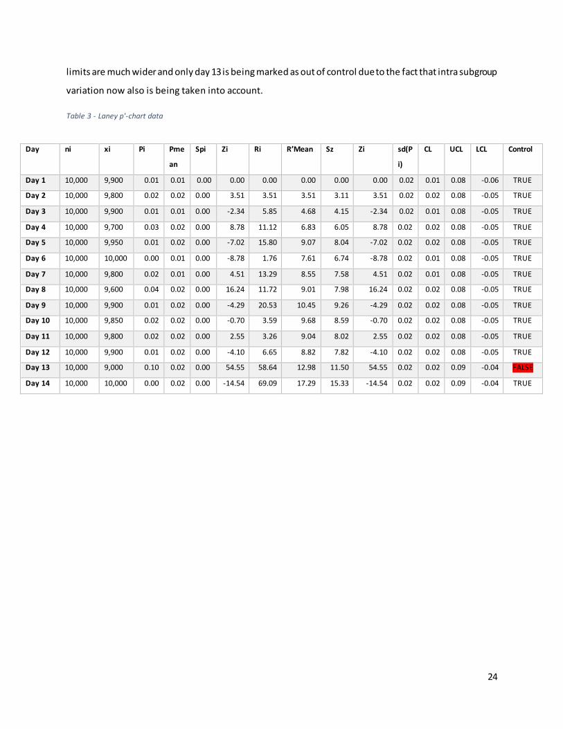
Applying this new approach to our toy problem from before yields the results that can be seen in Table 3

and Figure 9. The difference with the standard approach that is immediately visible is that the control

24

limits are much wider and only day 13 is being marked as out of control due to the fact that intra subgroup

variation now also is being taken into account.

Table 3 - Laney p'-chart data

Day ni xi Pi Pme

an

Spi Zi Ri R’Mean Sz Zi sd(P

i)

CL UCL LCL Control

Day 1 10,000 9,900 0.01 0.01 0.00 0.00 0.00 0.00 0.00 0.00 0.02 0.01 0.08 -0.06 TRUE

Day 2 10,000 9,800 0.02 0.02 0.00 3.51 3.51 3.51 3.11 3.51 0.02 0.02 0.08 -0.05 TRUE

Day 3 10,000 9,900 0.01 0.01 0.00 -2.34 5.85 4.68 4.15 -2.34 0.02 0.01 0.08 -0.05 TRUE

Day 4 10,000 9,700 0.03 0.02 0.00 8.78 11.12 6.83 6.05 8.78 0.02 0.02 0.08 -0.05 TRUE

Day 5 10,000 9,950 0.01 0.02 0.00 -7.02 15.80 9.07 8.04 -7.02 0.02 0.02 0.08 -0.05 TRUE

Day 6 10,000 10,000 0.00 0.01 0.00 -8.78 1.76 7.61 6.74 -8.78 0.02 0.01 0.08 -0.05 TRUE

Day 7 10,000 9,800 0.02 0.01 0.00 4.51 13.29 8.55 7.58 4.51 0.02 0.01 0.08 -0.05 TRUE

Day 8 10,000 9,600 0.04 0.02 0.00 16.24 11.72 9.01 7.98 16.24 0.02 0.02 0.08 -0.05 TRUE

Day 9 10,000 9,900 0.01 0.02 0.00 -4.29 20.53 10.45 9.26 -4.29 0.02 0.02 0.08 -0.05 TRUE

Day 10 10,000 9,850 0.02 0.02 0.00 -0.70 3.59 9.68 8.59 -0.70 0.02 0.02 0.08 -0.05 TRUE

Day 11 10,000 9,800 0.02 0.02 0.00 2.55 3.26 9.04 8.02 2.55 0.02 0.02 0.08 -0.05 TRUE

Day 12 10,000 9,900 0.01 0.02 0.00 -4.10 6.65 8.82 7.82 -4.10 0.02 0.02 0.08 -0.05 TRUE

Day 13 10,000 9,000 0.10 0.02 0.00 54.55 58.64 12.98 11.50 54.55 0.02 0.02 0.09 -0.04 FALSE

Day 14 10,000 10,000 0.00 0.02 0.00 -14.54 69.09 17.29 15.33 -14.54 0.02 0.02 0.09 -0.04 TRUE

25

Figure 12 - Laney p'-chart toy problem

Control charting algorithm for benchmarking

With the ability to identify which days are performing normally and which days are out of control we now

develop a new benchmarking approach that enables us to set targets for each second root cause level as

described in chapter 2.

For the algorithm that we developed there are a number of underlying assumptions which validate the

proposed approach:

1. Root causing is done properly by the Distribution Requirements Planning team.

2. Removing days that are out of control leaves a set of data which are in control and these represent

the stable state of the supply chain process.

The first step of the algorithm that we developed consists of calculating the control limits for a certain

period of time, the benchmark timespan. These control limits are calculated with the inter and intra

variance of the complete data set, this means the first data points is also adjusted for the variance that

occur in the latest day. After having the control limits ready we can then check each day that is present in

this against these limits and remove them from the set if they violate the limit.

-0.08

-0.06

-0.04

-0.02

0.00

0.02

0.04

0.06

0.08

0.10

0.12

1 2 3 4 5 6 7 8 9 10 11 12 13 14

Laney P'-chart Toy Problem

CL UCL LCL Pi

26

After having done these steps a new problem rises. Because the parameters on which the control limits

can be inflated massively by the days that are out of control and therefor giving us too loose limits we

need to develop an approach to define if we want to repeat the steps of removing out of control days for

a second time. In the academic literature there is no solution present for this problem and therefore we

have developed our own practical solution to have a solid algorithm with a clear rule of when to repeat

the steps.

Stop algorithm

As described above we have developed a rule of when to rerun the algorithm of removing out of control

days for a second time.

We propose introducing a new variable α that represents an allowance for the percentage of data points

that are out of control with the newly calculated control limits. If the number of data points that are out

of control after the removing them for the first time and recalculating control limits is lower than α we

iterate over the data set one more time to remove out of control days again.

The underlying idea behind this approach is that when there are a lot of points again out of control the

impact of the intra subgroup variance of the removed data points was relatively lower than when there

are only a few new data points out of control. And what we want to achieve is to remove the influence of

the first removed data points to obtain correct limits.

α = Allowance of data points out of control after first iteration

If after first iteration % of data points out control < α then remove days one more time.

The full algorithm applied on the toy problem looks as in the following tables and figures:

27

Step 1: Calculate performance of complete data set. Day 13 is being marked as out of control and the

mean performance of the complete set is 0.022 (2.2%)

Table 4 - step 1 algorithm toy problem

days cuts orders Pi Pmean Spi Zi Ri R'mean Sz Zi sd(Pi) UCL LCL CL Control?

Day 1 9,900 10,000 .010 .010 .001 .000 .000 .000 .000 .000 .024 .095 -.051 .022 TRUE

Day 2 9,800 10,000 .020 .015 .001 3.398 3.398 3.398 3.012 3.398 .024 .095 -.051 .022 TRUE

Day 3 9,900 10,000 .010 .013 .001 -2.265 5.663 4.531 4.016 -2.265 .024 .095 -.051 .022 TRUE

Day 4 9,700 10,000 .030 .018 .001 8.495 10.760 6.607 5.857 8.495 .024 .095 -.051 .022 TRUE

Day 5 9,950 10,000 .005 .015 .001 -6.796 15.291 8.778 7.782 -6.796 .024 .095 -.051 .022 TRUE

Day 6 10,000 10,000 .000 .013 .001 -8.495 1.699 7.362 6.527 -8.495 .024 .095 -.051 .022 TRUE

Day 7 9,800 10,000 .020 .014 .001 4.369 12.864 8.279 7.340 4.369 .024 .095 -.051 .022 TRUE

Day 8 9,400 10,000 .060 .019 .001 27.608 23.239 10.416 9.234 27.608 .024 .095 -.051 .022 TRUE

Day 9 9,900 10,000 .010 .018 .001 -5.663 33.271 13.273 11.767 -5.663 .024 .095 -.051 .022 TRUE

Day 10 9,850 10,000 .015 .018 .001 -2.039 3.624 12.201 10.817 -2.039 .024 .095 -.051 .022 TRUE

Day 11 9,800 10,000 .020 .018 .001 1.236 3.274 11.308 10.025 1.236 .024 .095 -.051 .022 TRUE

Day 12 9,900 10,000 .010 .018 .001 -5.097 6.333 10.856 9.624 -5.097 .024 .095 -.051 .022 TRUE

Day 13 9,000 10,000 .100 .024 .001 51.753 56.850 14.689 13.022 51.753 .024 .095 -.051 .022 FALSE

Day 14 10,000 10,000 .000 .022 .001 -15.048 66.801 18.698 16.576 -15.048 .024 .095 -.051 .022 TRUE

Figure 13 - graph first step algorithm toy problem

.022

Out of control

-.060

-.040

-.020

.000

.020

.040

.060

.080

.100

.120

Day 1 Day 2 Day 3 Day 4 Day 5 Day 6 Day 7 Day 8 Day 9 Day 10 Day 11 Day 12 Day 13 Day 14

Toy problem first calculation

UCL LCL CL Pi

28

.016

Out of control

-.030

-.020

-.010

.000

.010

.020

.030

.040

.050

.060

.070

Day 1 Day 2 Day 3 Day 4 Day 5 Day 6 Day 7 Day 8 Day 9 Day 10 Day 11 Day 12 Day 14

Toy problem 1st iteration

UCL LCL CL Pi

Figure 14- first iteration algorithm toy problem graph

Step 2: Remove the out of control point (day 13) and recalculate limits and the percentage of points that

are out of control. New mean performance of the set is 0.016 (1.6%).

The percentage of data points that are out of control is 7.69%.

Table 5- first iteration algorithm toy problem

days cuts orders Pi Pmean Spi Zi Ri R'mean Sz Zi sd(Pi) UCL LCL CL Control?

Day 1 9,900 10,000 .010 .010 .001 .000 .000 .000 .000 .000 .014 .057 -.025 .016 TRUE

Day 2 9,800 10,000 .020 .015 .001 3.966 3.966 3.966 3.516 3.966 .014 .057 -.025 .016 TRUE

Day 3 9,900 10,000 .010 .013 .001 -2.644 6.610 5.288 4.688 -2.644 .014 .057 -.025 .016 TRUE

Day 4 9,700 10,000 .030 .018 .001 9.915 12.559 7.712 6.837 9.915 .014 .057 -.025 .016 TRUE

Day 5 9,950 10,000 .005 .015 .001 -7.932 17.848 10.246 9.083 -7.932 .014 .057 -.025 .016 TRUE

Day 6 10,000 10,000 .000 .013 .001 -9.915 1.983 8.593 7.618 -9.915 .014 .057 -.025 .016 TRUE

Day 7 9,800 10,000 .020 .014 .001 5.099 15.015 9.664 8.567 5.099 .014 .057 -.025 .016 TRUE

Day 8 9,400 10,000 .060 .019 .001 32.225 27.126 12.158 10.778 32.225 .014 .057 -.025 .016 FALSE

Day 9 9,900 10,000 .010 .018 .001 -6.610 38.835 15.493 13.735 -6.610 .014 .057 -.025 .016 TRUE

Day 10 9,850 10,000 .015 .018 .001 -2.380 4.231 14.241 12.625 -2.380 .014 .057 -.025 .016 TRUE

Day 11 9,800 10,000 .020 .018 .001 1.442 3.822 13.199 11.702 1.442 .014 .057 -.025 .016 TRUE

Day 12 9,900 10,000 .010 .018 .001 -5.949 7.391 12.671 11.234 -5.949 .014 .057 -.025 .016 TRUE

Day 14 10,000 10,000 .000 .016 .001 -12.814 6.864 12.188 10.805 -12.814 .014 .057 -.025 .016 TRUE

29

.013

-.020

-.010

.000

.010

.020

.030

.040

.050

Day 1 Day 2 Day 3 Day 4 Day 5 Day 6 Day 7 Day 9 Day 10 Day 11 Day 12 Day 14

Toy problem last iteration

UCL LCL CL Pi

Figure 15 - Toy problem algorithm last iteration

Step 3: Compare the percentage of out of control data points to the set allowance α. If this is lower than

α then we iterate once more over the set removing new out of control days. If α in our toy problem

would be > 7.69% then we would iterate once more. If α < 7.69% the algorithm stops and we have the

targeted mean performance of the stable state as centre line.

For the purpose of showing the full algorithm we set α = 10.00% for our example and this gives us the

final results as follows.

The final target for the transportation process in the toy problem therefore is maximum 1.3%.

Table 6 - last iteration algorithm toy problem

days cuts orders Pi Pmean Spi Zi Ri R'mean Sz Zi sd(Pi) UCL LCL CL Control?

Day 1 9,900 10,000 .010 .010 .001 .000 .000 .000 .000 .000 .009 .039 -.014 .013 TRUE

Day 2 9,800 10,000 .020 .015 .001 4.500 4.500 4.500 3.990 4.500 .009 .039 -.014 .013 TRUE

Day 3 9,900 10,000 .010 .013 .001 -3.000 7.501 6.000 5.320 -3.000 .009 .039 -.014 .013 TRUE

Day 4 9,700 10,000 .030 .018 .001 11.251 14.251 8.751 7.758 11.251 .009 .039 -.014 .013 TRUE

Day 5 9,950 10,000 .005 .015 .001 -9.001 20.252 11.626 10.307 -9.001 .009 .039 -.014 .013 TRUE

Day 6 10,000 10,000 .000 .013 .001 -11.251 2.250 9.751 8.644 -11.251 .009 .039 -.014 .013 TRUE

Day 7 9,800 10,000 .020 .014 .001 5.786 17.037 10.965 9.721 5.786 .009 .039 -.014 .013 TRUE

Day 9 9,900 10,000 .010 .013 .001 -2.813 8.599 10.627 9.421 -2.813 .009 .039 -.014 .013 TRUE

Day 10 9,850 10,000 .015 .013 .001 1.500 4.313 9.838 8.721 1.500 .009 .039 -.014 .013 TRUE

Day 11 9,800 10,000 .020 .014 .001 5.400 3.900 9.178 8.137 5.400 .009 .039 -.014 .013 TRUE

Day 12 9,900 10,000 .010 .014 .001 -3.273 8.673 9.128 8.092 -3.273 .009 .039 -.014 .013 TRUE

Day 14 10,000 10,000 .000 .013 .001 -11.251 7.978 9.023 7.999 -11.251 .009 .039 -.014 .013 TRUE

30

Benchmark approach extended to Procter & Gamble case

Using the algorithm described in the section above we now have the ability to calculate a robust target

for each 2nd level root cause in the Procter & Gamble supply chain. With the data present we develope a

program that calculates the performance of each process over a timespan of the last X months, removing

all the days that are out of control. The average CuFR that is left is then the maximum allowed target for

the next month.

The underlying assumption in this approach is that when the company is able to perform on a certain level

for a number of months then the performance of the next month should be better or at least as good.

The created tool is run at the beginning of each month and automatically calculates the targets for each

process. In the creation of this process there are a number of parameters and settings that needs to be

set in the best possible way and is explained in the next part.

Developed program

For the new approach to be adopted as quick as possible we have developed an excel program that

automatically calculated the targets and performance for each process with one click. The owner of the

tool is the CFR-KU which runs the program on a monthly basis.

The program uses VBA and PowerPivot plugin (see Appendix B VBA Codes for full codes) to analyse the

data in an iterative way and outputs the results for each Supply Chain in a separate file. In this file the

Cluster leader for the specific supply chain then also has the ability to analyse area’s where the

performance is not sufficient using a deep dive analysis showing all the background information for the

cuts happened in a specific process.

In Figure 13, Figure 14 and Figure 15 we show for the transportation process of the months June, July and

August what the output of the algorithm is. We see that at the beginning the average CuFR is 0,162% and

after we applied the algorithm this is reduced to a stable state of 0.053%. From the graphs we can also

see that there is a huge volatility in the first graph Figure 13 that has been reduced significantly in Figure

14 and Figure 15 showing the cuts nicely moving around the mean and thus showing a stable state.

31

Figure 17 - Transportation process start (P = 0.162%)

Figure 16 - Transportation process first removal (P = 0.088%)

32

Figure 18 - Transportation process final results (P = 0.053%)

Parameter selection

The parameters and settings in the benchmark program that needed to be set are the following:

α = Allowance of number of data points out of control

X = Number of months to aggregate for benchmarking

Aggregating Western Europe supply chains versus calculating each supply chain individual

To be able to determine which settings should be used we developed a number of criteria which will help

is determine what settings are the most suitable for the needs of Procter & Gamble. These criteria are

developed in a number of work sessions with the supply chain leaders of Western Europe.

Table 7 - Criteria parameter selection

Criteria Importance

Run time ++

% of unexplained cuts target +

Data validity +++

With these criteria available for selecting the right parameters we have run number of different

calculations with all different settings in the tool.

33

First we see what the optimal timespan for which the data is used to benchmark the data against. We

have come up with 3 different options, using one, three or six months of data to calculate the targets.

These are scored against the three criteria that are showed in Table 7 - Criteria parameter selection. After

running with only one month of data we immediately saw that because there were too little data points

for the algorithm we dropped this option. The options for 3 and 6 months have been run afterwards and

yields the results shown in Table 9. What we can see from these results is that the 6 months run is

performing slightly better on “% of unexplained cuts target” (0.5237% versus 0.4334%). On data validity

we can deduct that because we have used a larger dataset with more data points the validity also is slightly

higher. On the other side the runtime of the 6 months variant versus the 3 months run was more than 3

times as high (20 minutes versus 60+ minutes). Putting these results in a cross table we can see that using

3 months of data is the most suitable for the criteria set by Procter & Gamble.

Table 8 - Scoring results vs criteria

Run time % of unexplained

cuts target

Data validity Total score

3 months 1 2 2 4

6 months 3 1 1 5

34

Table 9 - Results 3 versus 6 months

The next setting selection was to choose whether to aggregate the results of all Western Europe versus

to calculate each supply chain individually. Again we run both setups and compare the results against the

set criteria. We run the results for Northern Europe separately and for all Europe aggregated, the results

are shown in Table 11. Scoring the results on the criteria as before we find the results in Table 10. On all

criteria’s it is better to aggregate the data of the different supply chain to calculate targets. This is in line

with what we expected because there is significantly more data available due to the aggregation and the

run time is shorter because the analysis only has to be run once instead of for each supply chain

separately.

Root cause P-mean (3 months)

P-mean (6 months)

1.1 Master Data 0.0021% 0.0041% 1.10 Information/Tech Tools 1.2 Supply Planning Execution 0.0941% 0.0915% 1.3 Quality/Regulatory 0.0094% 0.0000% 1.4 Material Supply 0.0010% 0.0001% 1.5 Manufacturing Execution 0.0003% 1.6 Transport & Warehousing 0.0455% 0.0358% 1.7 Order Management 0.0001% 0.0001% 1.8 Other 0.0107% 0.0005% 1.9 Suppressed Demand-Sup Iss 2.1 Demand Planning 0.1640% 0.1678% 2.2 Initiatives Readiness 0.0750% 0.0068% 2.3 Capacity to Demand Strateg 0.0278% 0.0014% 2.4 Unplanned or Off-strategy 2.5 Other 0.0384% 0.0050% 2.6 Automated Availability Management (or shorted abbreviation) 2.9 Suppressed Demand-Bus Pln 3.1 Customer Operations 0.0012% 0.0005% 3.2 Mkt/customer forecast input 0.1007% 0.0837% 3.3 Communication to customer 3.4 Cust order out of policy 3.5 Other 0.0001% 3.9 Suppressed Demand-Comm Ex 7.1 Not Analysed 0.5237% 0.4334%

35

Table 10 - Scoring results versus criteria (2)

Run time % of unexplained

cuts target

Data validity Total score

Separate 3 2 2 5

Aggregated 1 1 1 3

Table 11 - Results Northern Europe versus Europe

Root cause P-mean NE P-mean EUR 1.1 Master Data 1.10 Information/Tech Tools 1.2 Supply Planning Execution 0.0154% 1.3 Quality/Regulatory 0.0016% 1.4 Material Supply 0.0070% 1.5 Manufacturing Execution 1.6 Transport & Warehousing 0.0215% 0.0467% 1.7 Order Management 1.8 Other 1.9 Suppressed Demand-Sup Iss 2.1 Demand Planning 0.0308% 2.2 Initiatives Readiness 0.0090% 2.3 Capacity to Demand Strateg 2.4 Unplanned or Off-strategy 2.5 Other 0.0130% 2.6 Automated Availability Management (or shorted abbreviation) 2.9 Suppressed Demand-Bus Pln 3.1 Customer Operations 3.2 Mkt/customer forecast input 0.0065% 0.0153% 3.3 Communication to customer 3.4 Cust order out of policy 3.5 Other 3.9 Suppressed Demand-Comm Ex 7.1 Not Analysed 0.4088% 0.5624%

For the last parameter (α) that needs to be set it is harder to define this with an experiment, as the

parameter does not significantly affects the run time or data validity. Next to this it not always have

influence on the % of unexplained cuts as it might differ per month if a second last iteration will be applied

based on the α. The results of running with an = 50% versus α = 20% can be seen in Table 12 and here we

36

can see that raising the value of alfa will give an extra iteration in more instances (1.2, 1.3 and 2.2 got an

extra iteration in the 50% run but not in the 20% run). After consulting with the supply chain leaders we

have decided to set the value of alpha to 20%.

Table 12 - Results 50% versus 20% alpha.

Root cause P-mean (50%)

P-mean (20%)

1.1 Master Data 0.0025% 0.0025% 1.10 Information/Tech Tools 1.2 Supply Planning Execution 0.0065% 0.0159% 1.3 Quality/Regulatory 0.0208% 0.0352% 1.4 Material Supply 0.0262% 0.0262% 1.5 Manufacturing Execution 0.0117% 0.0117% 1.6 Transport & Warehousing 0.0534% 0.0534% 1.7 Order Management 0.0007% 0.0007% 1.8 Other 0.0017% 0.0017% 1.9 Suppressed Demand-Sup Iss 2.1 Demand Planning 0.0690% 0.0690% 2.2 Initiatives Readiness 0.0124% 0.0261% 2.3 Capacity to Demand Strateg 2.4 Unplanned or Off-strategy 2.5 Other 0.0004% 0.0004% 2.6 Automated Availability Management (or shorted abbreviation) 2.9 Suppressed Demand-Bus Pln 3.1 Customer Operations 0.0004% 0.0004% 3.2 Mkt/customer forecast input 0.0690% 0.0690% 3.3 Communication to customer 0.0010% 0.0010% 3.4 Cust order out of policy 3.5 Other 3.9 Suppressed Demand-Comm Ex 7.1 Does not require Analysis 0.5497% 0.5497% 7.1 Waiting to be analysed 0.0342% 0.0342%

Conclusion

In this chapter we have developed a new approach to calculate stable state behaviour of processes. We

have shown that the standard P control chart is not feasible to use with the large sample data that is

present at Procter & Gamble because of underestimating inter subgroup variance. To overcome this issue

we have adopted the Laney P’ control chart that measures this variance and then adjust the control limits

for it.

37

With this approach we then have built a software program that automatically benchmarks the last month

performance against the previous 3 months and is able to identify which process is performing poorly and

should be improved in a robust and scalable way. The next step that needs to be taken is incorporate this

data in a drumbeat that ensures good control and improvement of non performing areas.

38

39

Chapter 4: Improve & Control The final steps in the DMAIC framework are the Improve and Control steps. As said this is where the real

strength of the methodology comes from and incorporates a review process that allows continuous

improvement and tracking of action plan performance. As input for this chapter we use the output from

the developed program which is shown in Figure 19 and Figure 20. In the last figure you can see that we

not only measure the MTD performance versus its target but we also calculate the amount of days that

the process was out of control, this is useful as second measure to see how big the problems are.

Actuals per Ownership

UK

Irel

and

Iber

ia

DAC

H

Ital

y G

roup

FBN

L

Nor

dic

Gra

nd T

otal

UK

Irel

and

Iber

ia

DAC

H

Ital

y G

roup

FBN

L

Nor

dic

Gra

nd T

otal

CFR Actual 98,72% 98,86% 98,76% 97,55% 99,38% 98,67% 98,68% 98,72% 98,86% 98,76% 97,55% 99,38% 98,67% 98,68%

CFR Target 98,50% 98,90% 99,00% 98,90% 99,00% 98,50% 98,20% 98,50% 98,90% 99,00% 98,90% 99,00% 98,50% 98,20%

Commercial Execution ,45% ,08% ,58% ,34% ,26% ,00% ,00% ,00% ,00% ,19% ,00% ,01%

Customer Operations ,11% ,02%

Demand Planning PSC ,16% ,03% ,37% ,28% ,08% ,17% -,06% ,04% -,04% -,02% ,01% -,06% -,05%

Doesn't require analysis. ,29% ,22% ,35% ,13% ,11% ,16% ,24% ,01% ,00% -,02% ,92% -,02% -,03% ,09%

Manufacturing Execution ,24% ,03% ,05% -,04% ,09% -,03% -,03% ,03% ,46% ,00%

Order Management ,04% ,01% ,00% ,00% ,24% ,00% ,03% ,00% ,04%

Others ,01% ,01% ,18% ,03% ,28% ,26% ,18% -,05% -,01% -,07% ,15%

QA Plant Driven ,04% ,02% ,94% ,13% ,00% ,00% ,04% ,00% ,00% ,00% ,01%

Supply Planning PSC ,20% ,20% ,31% ,50% ,12% ,01% ,00% ,01% ,00% ,00% ,00% ,00%

Transport & Warehousing ,34% ,31% ,23% ,00% ,04% ,23%

Waiting to be analyzed ,18% ,13% ,05% ,33% ,07% ,02% -,07% ,28% ,18% -,01% -,14% ,01%

-,05% -,04% -,03% ,14% -,03% -,05% -,04%

Target per OwnershipCommercial Execution ,07% ,05% ,05% ,05% ,05% ,07% ,08% ,00% ,00% ,00% ,00% ,00% ,00% ,00%

Customer Operations -,03% -,02% -,02% ,01% -,02% -,03% -,03%

Demand Planning PSC ,14% ,10% ,09% ,10% ,09% ,14% ,16%

Doesn't require analysis. ,96% ,70% ,64% ,70% ,64% ,96% 1,15%

Manufacturing Execution ,00% ,00% ,00% ,00% ,00% ,00% ,01% ,11% ,02%

Order Management ,00% ,00% ,00% ,00% ,00% ,00% ,00% ,38% -,02% -,05% ,53% -,05% ,27% ,17%

Others ,03% ,02% ,02% ,02% ,02% ,03% ,04% ,04% ,01%

QA Plant Driven ,03% ,02% ,02% ,02% ,02% ,03% ,04%

Supply Planning PSC ,16% ,12% ,11% ,12% ,11% ,16% ,19% ,15% ,02%

Transport & Warehousing ,07% ,05% ,05% ,05% ,05% ,07% ,08%

Waiting to be analyzed ,05% ,03% ,03% ,03% ,03% ,05% ,05% -,67% -,48% -,29% -,57% -,53% -,79% -,90%

-,05% ,14% -,03% ,10% ,02% ,28% ,02%

-,22% ,04% ,24% 1,35% -,38% -,17% -,48%

7.1 Does not require Analysis

7.1 Waiting to be analyzed

Individual SUM

3.2 Mkt/customer forcast input

3.3 Communication to customer

3.4 Cust order out of policy

3.5 Other

3.9 Suppressd Demand-Comm Ex

2.4 Unplanned or Off-strategy

2.5 Other

2.6 Automated Availailability Management (or shorted a

2.9 Suppressd Demand-Bus Pln

3.1 Customer Operations

1.8 Other

1.9 Suppressed Demand-Sup Iss

2.1 Demand Planning

2.2 Initiatives Readiness

2.3 Capacity to Demand Strateg

1.3 Quality/Regulatory

1.4 Material Supply

1.5 Manufacturing Execution

1.6 Transport & Warehousing

1.7 Order Management

CFR ActualCFR Target

1.1 Master Data

1.10 Information/Tech Tools

1.2 Supply Planning Execution

Actuals vs. Target per rootcause lvl 2

Figure 19 - Output from control chart benchmark tool (1)

40

Figure 20 - Output from control chart benchmark tool (2)

For improvement concerns one of the main requests was to present the data such that there was a clear

“accountability”. This means that from the results it must be immediately clear which team or department

is under performing and should take actions to get back on track. For the results from the second level

root causes to be accountable we assigned every 2nd level root cause to a specific owner, this allocation

can be seen in Table 13. The target and actual performance per ownership is then simply the sum of the

targets and actuals and is calculated in the benchmark tool automatically as well.

# of days OOC (UCL3)

UK

Irel

and

Iber

ia

DAC

H

Ital

y G

roup

FBN

L

Nor

dic

Gra

nt T

otal

CFR TargetsTarget (base)

UK

Irel

and

Iber

ia

DAC

H

Ital

y G

roup

FBN

L

Nor

dic

Gra

nd T

otal

1.1 Master Data 2 2 CFR Actual 98,72% 98,86% 98,76% 97,55% 99,38% 98,67% 98,68%

1.10 Information/Tech Tools CFR Target 98,50% 98,90% 99,00% 98,90% 99,00% 98,50% 98,20%

1.2 Supply Planning Execution 1 1 1 3 1.1 Master Data ,00% ,00% ,00% ,00% ,00% ,00% ,00% ,01%

1.3 Quality/Regulatory 2 1 6 9 1.10 Information/Tech Tools

1.4 Material Supply 3 1 4 8 1.2 Supply Planning Execution ,04% ,06% ,05% ,04% ,05% ,04% ,06% ,07%

1.5 Manufacturing Execution 5 2 7 1.3 Quality/Regulatory ,02% ,03% ,02% ,02% ,02% ,02% ,03% ,04%

1.6 Transport & Warehousing 3 4 3 1 11 1.4 Material Supply ,03% ,04% ,03% ,03% ,03% ,03% ,04% ,05%

1.7 Order Management 2 2 1.5 Manufacturing Execution ,00% ,00% ,00% ,00% ,00% ,00% ,00% ,01%

1.8 Other 1 1 2 1.6 Transport & Warehousing ,05% ,07% ,05% ,05% ,05% ,05% ,07% ,08%

1.9 Suppressed Demand-Sup Iss 1.7 Order Management ,00% ,00% ,00% ,00% ,00% ,00% ,00% ,00%

2.1 Demand Planning 4 4 2 1 11 1.8 Other ,00% ,00% ,00% ,00% ,00% ,00% ,00% ,00%

2.2 Initiatives Readiness 1 1 1.9 Suppressed Demand-Sup Iss

2.3 Capacity to Demand Strateg 2.1 Demand Planning ,09% ,14% ,10% ,09% ,10% ,09% ,14% ,16%

2.4 Unplanned or Off-strategy 2.2 Initiatives Readiness ,04% ,05% ,04% ,03% ,04% ,03% ,05% ,06%

2.5 Other 2 2 2.3 Capacity to Demand Strateg

2.6 Automated Availailability Management (or 2.4 Unplanned or Off-strategy ,00% ,00% ,00% ,00% ,00% ,00% ,00% ,00%

2.9 Suppressd Demand-Bus Pln 2.5 Other ,02% ,03% ,02% ,02% ,02% ,02% ,03% ,03%

3.1 Customer Operations 7 7 2.6 Automated Availailability Management (o

3.2 Mkt/customer forcast input 13 1 8 3 25 2.9 Suppressd Demand-Bus Pln

3.3 Communication to customer 5 5 3.1 Customer Operations

3.4 Cust order out of policy 3.2 Mkt/customer forcast input ,05% ,07% ,05% ,05% ,05% ,05% ,07% ,08%

3.5 Other 2 2 3.3 Communication to customer

3.9 Suppressd Demand-Comm Ex 3.4 Cust order out of policy

7.1 Does not require Analysis 3.5 Other

7.1 Waiting to be analyzed 4 2 1 3 10 3.9 Suppressd Demand-Comm Ex

Individual Sum 23 26 15 24 9 10 107 7.1 Does not require Analysis ,67% ,96% ,70% ,64% ,70% ,64% ,96% 1,15%

7.1 Waiting to be analyzed ,03% ,05% ,03% ,03% ,03% ,03% ,05% ,05%

Individual SUM 1,05% 1,50% 1,10% 1,00% 1,10% 1,00% 1,50% 1,80%

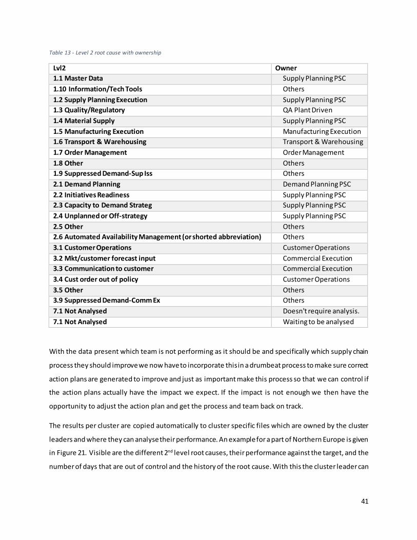
41

Table 13 - Level 2 root cause with ownership

Lvl2 Owner 1.1 Master Data Supply Planning PSC 1.10 Information/Tech Tools Others 1.2 Supply Planning Execution Supply Planning PSC 1.3 Quality/Regulatory QA Plant Driven 1.4 Material Supply Supply Planning PSC 1.5 Manufacturing Execution Manufacturing Execution 1.6 Transport & Warehousing Transport & Warehousing 1.7 Order Management Order Management 1.8 Other Others 1.9 Suppressed Demand-Sup Iss Others 2.1 Demand Planning Demand Planning PSC 2.2 Initiatives Readiness Supply Planning PSC 2.3 Capacity to Demand Strateg Supply Planning PSC 2.4 Unplanned or Off-strategy Supply Planning PSC 2.5 Other Others 2.6 Automated Availability Management (or shorted abbreviation) Others 3.1 Customer Operations Customer Operations 3.2 Mkt/customer forecast input Commercial Execution 3.3 Communication to customer Commercial Execution 3.4 Cust order out of policy Customer Operations 3.5 Other Others 3.9 Suppressed Demand-Comm Ex Others 7.1 Not Analysed Doesn't require analysis. 7.1 Not Analysed Waiting to be analysed

With the data present which team is not performing as it should be and specifically which supply chain

process they should improve we now have to incorporate this in a drumbeat process to make sure correct

action plans are generated to improve and just as important make this process so that we can control if

the action plans actually have the impact we expect. If the impact is not enough we then have the

opportunity to adjust the action plan and get the process and team back on track.

The results per cluster are copied automatically to cluster specific files which are owned by the cluster

leaders and where they can analyse their performance. An example for a part of Northern Europe is given

in Figure 21. Visible are the different 2nd level root causes, their performance against the target, and the

number of days that are out of control and the history of the root cause. With this the cluster leader can

42

identify which actions should be taken to increase each part that is underperforming. This file is updated

every month and a history of the action plan is being kept to see the impact of the actions taken.

To come to a reliable and feasible action plan the cluster leader dives into the processes that are out of

control (red) manually. We have added a page where the deep dive analysis can be done quickly by giving

an overview of the cuts and their background information, Figure 22, the data in this tool is presented in

SU rather than MSU for more accurate reporting. With this information at hand the cluster leader is able

to determine if there is already an action plan in place to improve the problems or if there is a need to

define new actions. In both cases the cluster leader have to make sure there is a final action present to

improve the process, either by copying the in place action or by escalating the problem to the accountable

team.

Rootcause lvl 2 Actual IX Owner Timing

OOC 0 0vs Target ,00% ,00%

OOC 0 0vs Target -,09% ,02%

OOC 0 -2vs Target -,02% -,03%

OOC 0 0vs Target -,01% ,00%

OOC 1 1vs Target ,04% ,04%

OOC 3 -1vs Target ,09% -,06%

vs Target History Actions

1.1 Master Data

1.2 Supply Planning Execution

1.3 Quality Regulatory

1.4 Material Supply

1.5 Manufacturing Execution

1.6 Transport & Warehousing

-,02%

,00%

,02%

-,50%

,00%

,50%

-,05%

,00%

,05%

-,02%

,00%

,02%

,04%

-,05%

,00%

,05%

-,20%

,00%

,20%

,40%

Figure 21 - Northern Europe cluster results example

43

Figure 22 - Cuts deep dive analysis

Control

To make sure the defined actions are executed properly and the impact is as projected we need to build

in a proper control structure. The drumbeat with reviews that is present at the moment is shown in Figure

23. As you can see there are a large number of periodical reviews that all focus on different part of

performance. We focus on the quarterly – monthly – weekly – daily reviews.

At the moment each periodic review has its own action plan that is being tracked separately. Due to this

setup the actions that are being developed in the monthly and quarterly meetings are not being tracked

on a regular basis and may lose impact. To overcome this problem in the new situation all actions that are

developed are put in a central action plan. This action plan is then reviewed during each weekly meeting

and this should improve the impact and success of the actions, Figure 24.

Slicer to select month, cluster and process Results are shown per DC

Actual cuts are shown grouped per 3rd level root cause. With all background

information present.

44

Figure 23 - Performance review drumbeat

Figure 24 - Old situation versus new situation

Daily Daily action plan

Weekly Weekly action plan

SNLT SNLT action plan

MonthlyMonthly

action plan

Weekly action plan

Daily

Monthly

SNLT

45

Results All the process adjustments that we developed are being implemented at Procter & Gamble at the

moment. Due to a transition of the Planning and Service Centre from Blois to Warsaw the first operational

month is in October after the internship and research has been finished and therefore we cannot give

actual results as of now.

The leadership team in the European Headquarter in Geneva received the proposed adjustments after we

presented the impact positively and therefore we are confident that this will help Procter and Gamble to

continuously improve the customer service with success.

The full recommendation and conclusions are summed up in the next chapter.

46

47

Conclusion and recommendations To answer the main research question that was stated in the problem statement we have developed five

sub questions that combined gives an answer on the main goal:

“How to improve service level and increase visibility and accuracy of tracking service losses per supply

chain process to enable continuous improvement.”

1. At what level of process detail do we need to improve tracking?

Measuring the performance at the process level is the most suited for the main goal, this means to

focus the tracking and analysis at the 2nd root cause level where the performance of each process is

aggregated. The 3rd root cause level is useful to understand what went wrong in the process.

2. How can we increase the visibility of achieved service level throughout the supply chain?

We developed a new reporting tool that gives deep dive capabilities to analyse each part of the supply

chain and zoom in or out of specific parts of interest.

3. How can we improve the accuracy in measuring performance of the processes?

By using control charting technique we are able to determine the stable state of each supply chain

process. Each month the process should perform just as good as or better than the stable

performance of the last 3 months. For this calculation we have developed a breakthrough algorithm

that automatically calculates the stable state performance using an adjusted Laney p control chart.

4. How can we identify actions to improve measured low performance?

We developed a tool in which each cluster leader can dive into the problems that occurred in his

supply chain and that are flagged by our algorithm as improvement area. By using all the background

information from multiple sources we are able to identify core problems in a fast way and developing

action plans with this information becomes an easy task.

5. Which process should be implemented to enable continuous improvement on service level using the

new tracking method? By using a centralized action plan that is fed by the daily, weekly, monthly and quarterly reviews each

action that is defined is tracked properly. Any deviation from the planning or impact of

implementation can be coped with immediately.

48

Recommendations We recommend the company to use the developed approach and processes in the HairCare category in

Europe for a first year and fine-tune the settings during this period. After this when the results are positive

the company can then easily extend the created tools to other categories because they are built to be

scalable and robust for any change, the only thing that needs to be adjusted is the report which exports

the results from the database to be able to deploy it in other businesses.

During this testing period I also recommend the company to do further research in the control rules to

use. At the moment we have only implemented the 3-sigma rule and even better results could possibly

be achieved by incorporating the full NELSON or WECO control rules. This needs to be investigated during

the actual usage by the owner of the tool (DRP leader).

One of the weaknesses that came up during the testing phase with the tools and have been identified is

that the use of Excel 2013 is a prerequisite of the tool. Because Microsoft does not support backward

compatibility between the Excel 2013 PowerPivot Plugin with any older version of Excel we are bound by

using this specific software package. As Microsoft is launching a new Excel version (2016) later this year it

is advisable to tale caution in using this as no information is present about compatibility between these

versions. My advice is to only open the tool in Excel 2013 to make sure nothing breaks.

All together this will result in improved measuring and tracking of service losses and together with detailed

action plans this results in a higher customer service level for the company.

49

Bibliography Champ, C., & Woodall, W. (2012). Exact Results for Shewhart Control Charts With Supplementary Runs

Rules. Technometrics, 393-399.

Eileen, M., van Aken, J., Farris, W., & Glover, G. (2010). A framework for designing, managing, and improving Kaizen event programs",. International Journal of Productivity and Performance Management, 641 - 667.

Howar, D. (n.d.). THE BASICS OF STATISTICAL PROCESS CONTROL & PROCESS BEHAVIOUR CHARTING. Management-NewStyle.

Laney, D. (2002). Improved Control Charts for Attributes. Quality Engineering, 531–537.

Lewis, B., & Mitchell, V. (2006). "Defining and Measuring the Quality of Customer Service. Marketing Intelligence & Planning, 11-17.

Liu, R., & Tang, J. (1996). Control Charts for dependent and independent Measurements based on Bootstrap method. Journal of the American Statistical Association, 1694-1700.

Nelson, L. (1984). The Shewhart Control Chart–Tests for Special Causes. Journal of Quality Technology, 237-239.

NIST/SEMATECH. (2015, 10 7). e-Handbook of Statistical Methods (WECO control rules). Retrieved from http://www.itl.nist.gov/div898/handbook/pmc/section3/pmc32.htm

Rever, H. (n.d.). Applying the DMAIC Steps to Process Improvement Projects. Internation Institute for Learning. Retrieved from International Institute for Learning.

Sanderson, E. (June 2015). NEW METHODS FOR CALCULATING OPTIMAL SAFETY STOCKS. Warsaw.

Schmitt, A. (2011). Strategies for customer service level protection under multi-echelon supply chain disruption risk. Supply chain disruption and risk management, 1266-1283.

Simchi-Levi, D. (2005). Safety Stock Positioning in Supply Chains with Stochastic Lead Times. Manufacturing & Service Operations Management, 295-318.

Woodall, W. (1997). Control charts based on attribute data: Bibliography and review. Journal of Quality Technology, 172-183.

50

51

Appendix A: Root cause tree

Level 1 Level 2 Level 3 Description

1.0 Supply Issues 1.1 Master Data 1.1.1 SIP Master Data SIP Master data requirements not communicated correctly or not maintained correctly

1.0 Supply Issues 1.1 Master Data 1.1.2 Category Master Data

Category Master Data requirements not communicated correctly or not maintianed correctly (i .e., Plants not triggered, trigger data base errors - trigger did not create materia l master views.)

1.0 Supply Issues 1.1 Master Data 1.1.3 MDO Master Data-2nd LvlD

MDO Master data requirements not communicated correctly or not maintained correctly for 2nd Level DC.

1.0 Supply Issues 1.1 Master Data 1.1.4 Order Mngmnt Master Data

OM Master data requirements not communicated correctly or not maintained correctly

1.0 Supply Issues 1.1 Master Data 1.1.5 DRP Master Data DRP master data requirements not communicated correctly or not maintained correctly

1.0 Supply Issues 1.1 Master Data 1.1.6 Dmnd Pln Sys Master Data Global Demand Forecast Convers ions

1.0 Supply Issues 1.10 Information/Tech Tools

1.10.1 gATP Functional i ty A system error resulting in a cut. For example: BOP job / filter variant failure due to masterdata not synched, MAD date incons is tency or other anomaly.

1.0 Supply Issues 1.10 Information/Tech Tools 1.10.2 gATP Cuts with Inv gATP cut at delivery creation when inventory i s confirmed to be available. For

example: Substitution did not invoke due to inaccuracy of supply elements.

1.0 Supply Issues 1.2 Supply Planning Execution

1.2.1 Excpt.Mess.not actioned

Exception messages were not actioned by the Planner.

1.0 Supply Issues 1.2 Supply Planning Execution

1.2.2 Excpt.Mess.not reviewed Exception messages were not reviewed by the Planner in a timely manner.

1.0 Supply Issues 1.2 Supply Planning Execution

1.2.3 SIP SWP

Planner did not follow the existing Standard Work Process (SWP), or in doing so was not consistent with the Plant Operating Strategy System (POSS). This could be due to training or other reasons such as: not taking appropriate actions on exception messages, Planner did not plan production to meet a SAFT requirement before a planned shutdown, Planner did not order material for a CM where planning i s owned by P&G, Planner scheduled production on the wrong l ine (l ine not qual i fied for the SKU.)

1.0 Supply Issues 1.2 Supply Planning Execution

1.2.4 Capacity Planning Error

Capacity planning error that doesn't protect current forecast (incl. promotions). This could be due to the Planner not performing capacity planning, not maintaining the C:D agreed in the POSS, or the capacity issue was not escalated for action by BOP.

1.0 Supply Issues 1.2 Supply Planning Execution

1.2.5 Safety Settng incorrect

Safety s tock settings were not maintained correctly or in a timely manner. This could be due to: 1) IP reviews not completed in the past 3 months 2) Incorrect assumptions were provided in support of the Inventory Target Setting process 3) Approved safety s tock settings not mainta ined correctly in SAP

1.0 Supply Issues 1.2 Supply Planning Execution

1.2.6 Phase In/Phs Out IOL SWP

Documented PIPO process not in-place, not sufficient or not fol lowed by IOL.

1.0 Supply Issues 1.2 Supply Planning Execution 1.2.7 DRP SWP

DRP Systems Issues and Work Process Failures which resulted in cut cases. 1) Inventory out of ba lance 2) planner execution 3) system failure 4) system does not meet bus iness need (LEO vis ibi l i ty)

52

1.0 Supply Issues 1.2 Supply Planning Execution

1.2.8 Si te Based DRP prcs fa i l Not fol lowing the SWP, master data and systems performance i s fine

1.0 Supply Issues 1.2 Supply Planning Execution

1.2.9 Glbl Plann SWP not fl lwd

Planner from another region did not follow the existing Standard Work Process (SWP) (i .e. cut occurred in sourcing or import region) or in doing so was not cons istent with the sourcing regions Operating Strategy. This could be due to tra ining or other reasons . (i .e. another region ordered too much)

1.0 Supply Issues 1.3 Qual ity/Regulatory 1.3.1 Supplier Quality Manage

Cases not ava ilable to ship due to out of specification material, regulatory compl iance and/or material quality i ssues associated with change or going production.

1.0 Supply Issues 1.3 Qual ity/Regulatory 1.3.10 Artwork Quality

1.0 Supply Issues 1.3 Qual ity/Regulatory 1.3.2 Manuf Quality - Micro

1.0 Supply Issues 1.3 Qual ity/Regulatory 1.3.3 Manuf Qual i ty/Regulatory

Cases not available to ship due to regulatory requirements and/or (in-process or finished product) was put on hold for inspection or rejected.

1.0 Supply Issues 1.3 Qual ity/Regulatory 1.3.4 Manipulation Quality Manipulated Cases/displays/special packs etc not available to ship due to regulatory requirements and/or (in-process or finished product) was put on hold for inspection or rejected.

1.0 Supply Issues 1.3 Qual ity/Regulatory 1.3.5 Expired Product Cases not available due to inabili ty to meet ship window date compl iance.

1.0 Supply Issues 1.3 Qual ity/Regulatory 1.3.6 Qual ity Release Exec Late release at DC or Plant due to warehouse qual i ty execution.

1.0 Supply Issues 1.3 Qual ity/Regulatory 1.3.7 Product damage quality i s sue(not due to Trans or pick)

1.0 Supply Issues 1.4 Materia l Supply 1.4.1 Insuf Supplier Capaci ty

Insufficient supplier capacity planned to protect current forecast plus C:D agreed in the SLEA (MSM/MSMAs)

1.0 Supply Issues 1.4 Materia l Supply 1.4.3 MSM SWP not Fol lowed SLEA didn't meet bus iness needs

1.0 Supply Issues 1.4 Materia l Supply 1.4.4 SLEAs not fol lowed Vendor Si te Level Execution Agreement expectations not fol lowed

1.0 Supply Issues 1.4 Materia l Supply 1.4.6 Supplier Execution Mnfg

Supplier under-delivered or delivered late due to supplier planning or manufacturing fa i lures

1.0 Supply Issues 1.4 Materia l Supply 1.4.7 Natura l Disaster-Supply

No supply due to natural disaster at the supplier or natural disaster impacted supplier's supplier - and the supplier was unable to produce P&G requirements.

1.0 Supply Issues 1.5 Manufacturing Execution

1.5.1 Manufact. Execut. MPSA

Under production or late production due to manufacturing execution. i.e. schedule was i ssued but product was not ava i lable on-time

1.0 Supply Issues 1.5 Manufacturing Execution

1.5.2 Mnfg Exct Data Integri ty

Product was not produced because there was less bulk or packaging inventory than what was stated in the system and as a result there was insufficient bulk or packaging for production.

1.0 Supply Issues 1.5 Manufacturing Execution

1.5.3 Manip.Execut. - MPSA Under production or late production due to manipulation execution.

1.0 Supply Issues 1.5 Manufacturing Execution

1.5.4 Natura l Disaster–No Manf

A natural disaster at the P&G production s ite has prevented or s ignificantly dis rupted the production output.

1.0 Supply Issues 1.5 Manufacturing Execution 1.5.5 Technical Readiness CPS supported Technical Readiness but manufacturing execution did not deliver.

1.0 Supply Issues 1.5 Manufacturing Execution

1.5.6 Logis t/Supp. Readiness

Under or late production/shipment of new initiatives due to supply chain start-up i ssues

1.0 Supply Issues 1.5 Manufacturing Execution

1.5.7 Product Comp. not ava i l Component Materia ls are not ava i lable.

1.0 Supply Issues 1.5 Manufacturing Execution

1.5.8 Late i ssue of document.

Approval documentation was not i s sued on time resulting in availability i s sues .(LAZ/AED)

1.0 Supply Issues 1.6 Transport & Warehous ing 1.6.1 IRA discrepancy Inventory Record Accuracy Issues resul ting in less s tock than expected.

53

1.0 Supply Issues 1.6 Transport & Warehous ing 1.6.10 Stolen Product Ful l Truck s tolen or individual product s tolen from truck.

1.0 Supply Issues 1.6 Transport & Warehous ing

1.6.11 Prod.Damage /Transport Product returned due to damage during the transportation process .

1.0 Supply Issues 1.6 Transport & Warehous ing

1.6.12 Prod.Damaged - Picking Product damaged during the picking process .

1.0 Supply Issues 1.6 Transport & Warehous ing

1.6.13 Wrong Product Picked Wrong product shipped by DC. Does not match the product ordered.

1.0 Supply Issues 1.6 Transport & Warehous ing

1.6.14 Paperwork Incomplete

Customer rejected product due to insufficient supporting documentation, such as shipping paperwork or QI documentation.

1.0 Supply Issues 1.6 Transport & Warehous ing 1.6.15 Late Del ivery Product del ivered to customer too late and customer refuses to accept.

1.0 Supply Issues 1.6 Transport & Warehous ing

1.6.16 Cust.Pickup-Truck Size

Customer Vehicle/Truck i s the wrong s ize for the ordered quanti ty.

1.0 Supply Issues 1.6 Transport & Warehous ing

1.6.17 Shipment Loading Error

Includes load building work process, overweight, master data, or physical load process. Where product is cut from a load at the DC prior to shipment known as 'Truck Sizing Corrections '

1.0 Supply Issues 1.6 Transport & Warehous ing

1.6.18 Product cut by carrier

Product originally shipped by P&G is cut by the carrier due to downstream manipulation such as re-pa l leti zing.

1.0 Supply Issues 1.6 Transport & Warehous ing

1.6.2 Ware.Sys./Process error Warehouse systems or Process Errors .

1.0 Supply Issues 1.6 Transport & Warehous ing

1.6.3 Outs ide s torage fa i lure Fa i lure in the outs ide s torage location resul ted in cuts to the shipment.

1.0 Supply Is sues 1.6 Transport & Warehous ing

1.6.4 Com.iss. -MP/Plant / DC

Communication i ssues between Market Planning, Plant and DC

1.0 Supply Issues 1.6 Transport & Warehous ing 1.6.5. DC breakdown Product not available for shipping due to a failure of warehouse equipment.

1.0 Supply Issues 1.6 Transport & Warehous ing

1.6.6 Inbound haulier Is sue

Constraint in interplant shipping impacting our ability to get sufficient product to the DC to meet demand, for example weather disruption on the inbound journey.

1.0 Supply Issues 1.6 Transport & Warehous ing

1.6.7 Customs Clearance Delay

Product not available for shipping due to customs clearance issues inbound to the ship-s i te or outbound to the customer.

1.0 Supply Issues 1.6 Transport & Warehous ing

1.6.8 In-transit LT Incorrect

Product shipped, but not received properly at the DC. The DC is unaware that the product was shipped.

1.0 Supply Issues 1.6 Transport & Warehous ing

1.6.9 Delay in transit-issue

Delay of the in-transit product. For example : • Product shipped on time, but delayed in transit. • Product shipped on time, but DC was delayed in processing the receipt. • Delay during shipment to and from contract manufacturers for manipulation.

1.0 Supply Issues 1.7 Order Management 1.7.1 Manual Entry Error Manual Entry Error

1.0 Supply Issues 1.7 Order Management

1.7.2 Insufficient Leadtime Order cut due to i tems with insufficient lead time to produce and/or ship.

1.0 Supply Issues 1.7 Order Management

1.7.3 Systems Error/Interface

A system error resulting in a cut. For example : Line i tem dropped from customer's order during acquis i tion of the order from the customer.

1.0 Supply Issues 1.7 Order Management

1.7.4 Delay-New Code or Sub Incomplete or late setup of new code or substi tution

1.0 Supply Issues 1.8 Other 1.8.1 Not covered in 1.0 This root cause code is provided to avoid excessive time loss trying to force fit the i ssue into one of the root causes above.

1.0 Supply Issues 1.9 Suppressed Demand-Sup Iss

1.9.1 Suppressd Demand-Sup Iss

Production capacity or supply of raw and packing materials insufficient to meet demand.

2.0 Business Planning Issues 2.1 Demand Planning

2.1.1 Demand Planning SWP Demand Planner did not esca late when demand inputs were insufficient

54

2.0 Business Planning Issues 2.1 Demand Planning 2.1.2 Communication:

Demand Er Planner received forecast input but fa i led to enter into the system

2.0 Business Planning Issues

2.1 Demand Planning 2.1.3 Wkly demnd mgmnt/cntrl

Cuts caused by Weekly Demand (Near-term) Maintenance, DFU level overshipments and/or control not performed/performed poorly (i .e. bias not managed through DDS process )

2.0 Business Planning Issues 2.1 Demand Planning

2.1.4 Sys maint/interface fa i l Data System fa i lure ei ther into DP system or from DP system

2.0 Business Planning Issues

2.2 Ini tiatives Readiness 2.2.1 CPS Management

CPS did not a l low sufficient time to complete tasks or delayys were not highlighted early enough to prevent impact on end date due to scope change, incorrect specs , etc.

2.0 Business Planning Issues

2.2 Ini tiatives Readiness

2.2.2 CMK underestimated Cnsmr

Underestimation of the consumer’s response to the new ini tiative.

2.0 Business Planning Issues

2.2 Ini tiatives Readiness

2.2.3 Market Plan chng not com

Marketing plan changes not communicated or communicated too late to demand planning that resul ted in cuts .

2.0 Business Planning Issues

2.2 Ini tiatives Readiness

2.2.4 Ini tiative fore not in Demand planning did not get the ini tiative forecast into the forecast tool .

2.0 Business Planning Issues

2.2 Ini tiatives Readiness 2.2.5 Planner human error Planner did not fol low s tandard work process .

2.0 Business Planning Issues

2.2 Ini tiatives Readiness 2.2.6 Artwork Planning Artwork process i s sues for new ini tiatives or promotions

2.0 Business Planning Issues

2.2 Ini tiatives Readiness

2.2.7 Project team Execution

Insufficient base plan, gtm plan, infeasible off quality Ie. 'incorrect demand process inputs '

2.0 Business Planning Issues

2.3 Capacity to Demand Strateg

2.3.1 Capty to Demand Strategy

C:D s trategy insufficient due to 1) Aligned C:D targets set incorrectly (too low), 2) C:D targets not defined & documented in the Category Operating Strategy, 3) Plant Operating Strategy not a l igned to Category C:D Strategy, 4) operating/inventory strategy not built off of demonstrated performance 5) Need for change in capaci ty or s trategy not addressed

2.0 Business Planning Issues

2.3 Capacity to Demand Strateg

2.3.2 Planned Capacity Not Real i zed RCCP i ssues addressed in BOP but plan not executed as expected.

2.0 Business Planning Issues

2.4 Unplanned or Off-s trategy

2.4.1 P&G Mngmnt Decis ion chg

P&G Management decision making/influence caused cuts. Issue identified and BU proceeds with ri sk (ex: reduce safety s tock for FYE inventory)

2.0 Business Planning Issues

2.4 Unplanned or Off-s trategy

2.4.2.Unplan demand-price chng

Unplanned demand from short-notice price changes

2.0 Business Planning Issues

2.4 Unplanned or Off-s trategy

2.4.3Unplan demand-tax/lega l

Unplanned demand from short-notice tax, lega l or customs changes

2.0 Business Planning Issues

2.4 Unplanned or Off-s trategy

2.4.5 Glbl BP Prcss not fl lwd

Global Supply Chain Planning Processes and Strategies (e.g., Import/Export assumptions not communicated or executed properly, export demand communication misses, capacity planning gaps across regions, overshipment of one country impacting the ava i labi l i ty in another country, etc.)

2.0 Business Planning Issues

2.4 Unplanned or Off-s trategy

2.4.6 Lega l chngs, artwork inv

Due to a short-notice local government legal change, artwork no longer meets regulatory requirements, stock i s placed on hold and unavai lable to ship.

2.0 Business Planning Issues 2.5 Other 2.5.1 Not covered in 2.0 This root cause code is provided to avoid excessive time loss trying to force fit

the i ssue into one of the root causes above.

2.0 Business Planning Issues

2.6 Automated Avai lailability Management (or shorted abbreviation)

2.6.1 Cut without Adv notice

Avai lability Management master data i s missing or incorrectly configured caus ing cuts to occur where the planning teams have no advance visibility of the requirement via the Avai labi l i ty Managent cycle

2.0 Business Planning Issues

2.9 Suppressd Demand-Bus Pln

2.9.1 Suppressd Demand-Bus Pln

Demand forecast was s ignificantly lower than the actual demand. • Constraint in interplant shipping impacting our ability to get sufficient product to the DC to meet demand.

55

3.0 Commercial Execution Issue

3.1 Customer Operations

3.1.1 Cst ordr out of guidel in

Order submitted with errors due to customer's maintenance of their ordering tables (e.g., combining products that should not be combined, incorrect unit of measure, obsolete product, exceeding truckload l imit.)

3.0 Commercial Execution Issue

3.1 Customer Operations

3.1.2 Cust order incorrect pro Customer submitted an order to P&G for the wrong product.

3.0 Commercial Execution Issue

3.1 Customer Operations

3.1.3 Cst order incorrect pric Customer inadvertently placed the order with the wrong price.

3.0 Commercial Execution Issue

3.1 Customer Operations

3.1.4 Cst ordr outside of date

Customer submitted the order to ship before the agreed/published new item or promotion fi rs t ship date.

3.0 Commercial Execution Issue

3.1 Customer Operations

3.1.5 Space/condition at rcvng

Customer's warehouse not able to receive the product due to insufficient space or inadequate conditions .

3.0 Commercial Execution Issue

3.1 Customer Operations

3.1.6 Sys mal function at rcvng

Customer's receiving information system not able to receive the product due to incorrect system setup or inaccurate bar code reading.

3.0 Commercial Execution Issue

3.1 Customer Operations 3.1.7. Cust financial s tatus Order cut due to a credit risk based upon customer's financial/payment s tatus .

3.0 Commercial Execution Issue

3.2 Mkt/customer forcast input

3.2.1 CBD input-Demand/Mkt Pln

CBD input provided to Demand/Market Planning was incorrect or missing (e.g. dates, products , pricing, quantity, etc.) - Incremental Business Assessment (IBA) process not fol lowed (quantity or timing) - Unforecasted, customer-generated demand increase without sufficient lead time. - Significantly overshipped event vs . the forecast provided to Demand/Market Planning.

3.0 Commercial Execution Issue

3.2 Mkt/customer forcast input

3.2.2 Cust chng qty post-windo

Customer or Customer Team increased/ changed the date of product demand quantity (beyond safety & buffer & s trategy) or sku split without proper notice. May be due to Event/Feature execution (e.g., feature/event announced on the wrong SKU.) ie. Customer communicated requirement though shipped later than what was communicated

3.0 Commercial Execution Issue

3.2 Mkt/customer forcast input

3.2.3 Cust Didnt Comm Event

Customer failed to provide appropriate information on event causing cuts (i.e Dis tribution changes , events , inventory adjustments , etc.)

3.0 Commercial Execution Issue

3.2 Mkt/customer forcast input

3.2.4 Unplan demand-cust/compe

Unplanned demand from short-notice of customer changes (e.g., response to competitive opportunities such as a failure of a competitor to fulfill the volume needed for a display event, so at the last minute the customer asks us to ship them our product displays to fi l l the event.

3.0 Commercial Execution Issue

3.3 Communication to customer

3.3.1 Incorrect prd ordr-PG er

P&G had not communicated correct product information - incorrect product code ordered

3.0 Commercial Execution Issue

3.3 Communication to customer

3.3.2 Prd over a l locatn-PG err

P&G had not communicated correct allocation information - product ordered above a l location

3.0 Commercial Execution Issue

3.3 Communication to customer

3.3.3 Prod ord out of ship win

P&G had not communicated correct dates - product ordered out of shipping window

3.0 Commercial Execution Issue

3.4 Cust order out of pol icy

3.4.1 Cust. not execute a l loc Customer ordered more than the communicated ava i lable s tock.

3.0 Commercial Execution Issue

3.4 Cust order out of pol icy

3.4.2 Order exceed promo a l lot

Orders cut due to customers not respecting the P&G communicated promotion a l lotment quantities (e.g., we have a planned, l imited amount of a special product that we are producing or in NA - Orders made outside of SPS submitted forecast.) BU s tated they couldn't support and customer ordered anyway.

3.0 Commercial Execution Issue

3.4 Cust order out of pol icy

3.4.3 Order exceed price a l lot

Orders cut due to customers not respecting the a llocated order quantitiies during a price change period.

3.0 Commercial Execution Issue

3.4 Cust order out of pol icy

3.4.4 Commercial Issue-Price

Customer used an old price even though they have the new price. A commercial i s sue needs to be addressed with the customer.

3.0 Commercial Execution Issue 3.5 Other 3.5.1. Not covered in 3.0 This root cause code is provided to avoid excessive time loss trying to force fit

the i ssue into one of the root causes above.

56

3.0 Commercial Execution Issue

3.9 Suppressd Demand-Comm Ex

3.9.1 Suppressed Demand-Comm E Suppressed Demand due to erroneous Commercia l Execution

7.0 Not Analyzed 7.1 Not Analyzed 7.1.1. Waiting to be analyzed Cuts that are s ti l l to be analysed.

7.0 Not Analyzed 7.1 Not Analyzed 7.1.2. Does not Require Anal .

Cuts that are automatically closed based on filter rules set up in the root causing tool . Typica l ly very smal l volume cuts .

57

Appendix B VBA Codes

Code for Report updates Public newupdatedate As Date Public lastupdatedate As Date Public databaselocation As String Public AllowedToContinue As Boolean Public updatebrandmatrix As Boolean Public optimus As String Sub RefreshALL() 'refresh the complete datamodel 'please run when geography or other support matrixes have been updated starttime = Timer Application.ScreenUpdating = False Application.EnableEvents = False ActiveWorkbook.Model.refresh Application.ScreenUpdating = True Application.EnableEvents = True endtime = Timer Msgbox "The data has been refreshed: " & (endtime - starttime) / 60 & " minutes" End Sub Sub CopyDatabaseLocal() Dim DirFile As String DirFile = "c:\OptimusPrime Database\OptimusPrime-DB.accdb" 'if the database is non existing download If Len(Dir(DirFile)) = 0 Then On Error Resume Next MkDir "C:\OptimusPrime Database" FileCopy databaselocation, "c:\OptimusPrime Database\OptimusPrime-DB.accdb" 'if the database is older than the one on the server replace it ElseIf FileDateTime(databaselocation) > FileDateTime("c:\OptimusPrime Database\OptimusPrime-DB.accdb") Then Dim fso As Object Set fso = VBA.CreateObject("Scripting.FileSystemObject") Call fso.CopyFile(databaselocation, "c:\OptimusPrime Database\OptimusPrime-DB.accdb", True) End If End Sub Sub progress(pctCompl As Single) 'updates the progressbar UserForm1.Text.Caption = pctCompl & "% Completed" UserForm1.Bar.Width = pctCompl * 2

58

DoEvents End Sub Sub start() 'opens the progressbar and starts the importdata macro (in the userform code) optimus = ActiveWindow.Caption UserForm1.Show End Sub Sub MonthClosing() If Msgbox("This will aggregate the data from daily to monthly for " & monthname(month(Date) - 2, mmm) & " and send the month closing report for " & monthname(month(Date) - 1, mmm) & ". Are you sure?", vbYesNo) = vbNo Then Exit Sub optimus = ActiveWindow.Caption 'archive the data archivedate 'Delete the data at daily level for Month-2 AggregateMonths 'Upload the database uploadDB 'Send month closing email sendcomplexemailattachmentmonthclosing End Sub Sub ImportData() Dim pctCompl As Single Dim maxk, k As Integer starttime = Timer 'progress BAR maxk = 6 k = 0 pctCompl = Round((100 / maxk) * k, 0) progress pctCompl 'if both downloaded workbooks are open and the name is correct and it is not monday If (Check_If_Workbook_Open("CFR-Daily-Cuts.xlsx")) And (Check_If_Workbook_Open("CFR-Daily-Orders.xlsx")) Then Msgbox "The update process is starting now. Please wait for the message that it is finished" Application.EnableEvents = False Application.ScreenUpdating = False

59

databaselocation = Worksheets("Update").Range("C30").Value updatebrandmatrix = False 'Copy the database locally CopyDatabaseLocal '''''''''''''' 'progress BAR' '''''''''''''' pctCompl = Round((100 / maxk) * k, 0) k = k + 1 progress pctCompl 'unprotect the sheets If Worksheets("Daily Report").ProtectContents = True Then Worksheets("Daily Report").Unprotect End If If Worksheets("Deepdive Analysis").ProtectContents = True Then Worksheets("Deepdive Analysis").Unprotect End If 'set the last updatedate to compare with Worksheets("Daily Report").Activate lastupdatedate = Worksheets("Daily Report").Range("C1").Value 'Step 1: update the Cuts data AddCutsToAccess ImportCutsTime = Timer 'Step 2: update the Orders data AddOrdersToAccess ImportShipmentsTime = Timer '''''''''''''' 'progress BAR' '''''''''''''' pctCompl = Round((100 / maxk) * k, 0) k = k + 1 progress pctCompl 'Step 3: Refresh the PowerPivot Windows("OptimusPrime - CFR Report.xlsm").Activate 'refresh Dates Windows("OptimusPrime - CFR Report.xlsm").Activate ActiveWorkbook.Model.ModelTables("date").refresh DoEvents If updatebrandmatrix = True Then Windows("OptimusPrime - CFR Report.xlsm").Activate ActiveWorkbook.Model.ModelTables("BrandDetailMatrix").refresh End If 'refresh Cuts Windows("OptimusPrime - CFR Report.xlsm").Activate

60

ActiveWorkbook.Model.ModelTables("AccessCuts").refresh DoEvents '''''''''''''' 'progress BAR' '''''''''''''' pctCompl = Round((100 / maxk) * k, 0) k = k + 1 progress pctCompl 'refresh Orders Windows("OptimusPrime - CFR Report.xlsm").Activate ActiveWorkbook.Model.ModelTables("AccessOrders").refresh DoEvents 'refresh FPC list Windows("OptimusPrime - CFR Report.xlsm").Activate Sheets("Products - Customers").Activate ActiveSheet.PivotTables("PivotTable1").PivotCache.refresh ActiveWorkbook.Model.ModelTables("Table10").refresh refreshtables = Timer '''''''''''''' 'progress BAR' '''''''''''''' pctCompl = Round((100 / maxk) * k, 0) k = k + 1 progress pctCompl 'update the last update date with todays update Worksheets("Daily Report").Activate Worksheets("Daily Report").Range("C1") = newupdatedate 'Step 4: refresh the filters to get the latest day updateDateFilters UpdateFilterTime = Timer 'Save the workbook ActiveWorkbook.Save '''''''''''''' 'progress BAR' '''''''''''''' pctCompl = Round((100 / maxk) * k, 0) k = k + 1 progress pctCompl 'Upload DB to the L drive uploadDB uploadDBTime = Timer '''''''''''''' 'progress BAR'

61

'''''''''''''' pctCompl = Round((100 / maxk) * k, 0) k = k + 1 progress pctCompl 'Copy the file to the sharepoint savecopy UploadSP = Timer '''''''''''''' 'progress BAR' '''''''''''''' pctCompl = Round((100 / maxk) * k, 0) k = k + 1 progress pctCompl 'Send email sendcomplexemailattachment 'Show the information about the update proces endtime = Timer Msgbox "Everything went okay! The time the steps took: " & Round((endtime - starttime) / 60, 2) & " minutes" _ & vbNewLine & _ "Import Cuts: " & Round((ImportCutsTime - starttime) / 60, 2) & " minutes" & vbNewLine & _ "Import Shipments: " & Round((ImportShipmentsTime - ImportCutsTime) / 60, 2) & " minutes" & vbNewLine & _ "RefreshTables: " & Round((refreshtables - ImportShipmentsTime) / 60, 2) & " minutes" & vbNewLine & _ "Update Filter: " & Round((UpdateFilterTime - refreshtables) / 60, 2) & " minutes" & vbNewLine & _ "Upload DB: " & Round((uploadDBTime - UpdateFilterTime) / 60, 2) & " minutes" & vbNewLine & _ "Upload Sharepoint: " & Round((UploadSP - uploadDBTime) / 60, 2) & " minutes" Application.EnableEvents = True Application.ScreenUpdating = True 'if only the cuts are open ElseIf (Check_If_Workbook_Open("CFR-Daily-Cuts.xlsx")) Then Msgbox "The workbook [CFR-Tool-Orders.xlsx] is not open or is not named correctly." End ' if only the orders are open ElseIf (Check_If_Workbook_Open("CFR-Daily-Orders.xlsx")) Then Msgbox "The workbook [CFR-Tool-Cuts.xlsx] is not open or is not named correctly." End 'if non of them are open

62

Else Msgbox "Both workbooks [CFR-Tool-Cuts.xlsx] and [CFR-Tool-Orders.xlsx] are not open or are not named correctly." End End If End Sub Sub uploadDB() 'save the newly updated database to the location where this is stored Dim fso As Object Windows(optimus).Activate databaselocation = Worksheets("Update").Range("C30").Value Set fso = VBA.CreateObject("Scripting.FileSystemObject") Call fso.CopyFile("c:\OptimusPrime Database\OptimusPrime-DB.accdb", databaselocation, True) End Sub Sub savecopy() 'save a copy of the report to the sharepoint databaselocation = Worksheets("Update").Range("C30").Value Application.DisplayAlerts = False Worksheets("Daily Report").Activate ActiveWorkbook.SaveAs "http://dcsp.pg.com/bu/PSCGlobal/PSC_Europe_TC/Document%20Library/EU%20Categories/Hair%20Care/Category-CFR/1.%20CFR%20report/OptimusPrime%20-%20CFR%20REPORT " & Format(Now, "DD-MMM") & ".xlsm" Application.DisplayAlerts = True End Sub Sub AddCutsToAccess() 'Macro to import the data from the fresh data extract into the dashboard 'For the macro to run it is required that the CFR-Data-Cuts.xlsx file is open Dim strMyPath As String Dim strDelete As String Windows("CFR-Daily-Cuts.xlsx").Activate strMyPath = Application.ActiveWorkbook.path strDelete = strMyPath & "\" & "CFR-Daily-Cuts.xlsx" 'format new data as table ActiveSheet.ListObjects.Add(xlSrcRange, Range(Cells(1, 1), Cells(xlLastRow, 12)), , xlYes).Name _ = "Table1" 'add calculated date in new column, weekend will be allocated to friday Range("K2").Select ActiveCell = _ "=IF(EOMONTH(DATEVALUE([@Time]),0)<TODAY(),EOMONTH(DATEVALUE([@Time]),0),IF(IF(WEEKDAY((TODAY()-1),3)=6,TODAY()-3,IF(WEEKDAY((TODAY()-1),3)=5,TODAY()-2,TODAY()-1))<DATEVALUE([@Time]),DATEVALUE([@time]),IF(WEEKDAY((TODAY()-1),3)=6,TODAY()-3,IF(WEEKDAY((TODAY()-1),3)=5,TODAY()-2,TODAY()-1))))" 'set the new update date to store when everything went okay

63

newupdatedate = Application.WorksheetFunction.max(Range(Cells(2, 11), Cells(xlLastRow, 11))) 'blank check Range("L2").Select ActiveCell = _ "=IF([@[Brand Detail]]=" & Chr(34) & Chr(34) & ",,VLOOKUP([@[Brand Detail]],'[OptimusPrime - CFR REPORT.xlsm]Products - Customers'!$A:$A,1,0))" 'if blank then pause macro to allow user interaction If Application.WorksheetFunction.CountIf(Range("L:L"), "#N/A") > 0 Then ActiveSheet.ListObjects("Table1").Range.AutoFilter Field:=12, Criteria1:="=#N/A" Application.ScreenUpdating = True Msgbox ("Please follow the instructions on the update tab for BLANKS") Pause updatebrandmatrix = True Application.ScreenUpdating = False End If 'clear filter again Windows("CFR-Daily-Cuts.xlsx").Activate ActiveSheet.ListObjects("Table1").Range.AutoFilter Field:=12 'set the new update date to store when everything went okay newupdatedate = Application.WorksheetFunction.max(Range(Cells(2, 11), Cells(xlLastRow, 11))) MoveDataToAccess ("AccessCuts") 'close and delete Windows("CFR-Daily-Cuts.xlsx").Close False Kill strDelete End Sub Sub AddOrdersToAccess() 'Macro to import the data from the fresh data extract into the dashboard 'For the macro to run it is required that the CFR-Data-Cuts.xlsx file is open Dim strMyPath As String Dim strDelete As String Dim str As String Dim count As Integer Application.ScreenUpdating = False Windows("CFR-Daily-Orders.xlsx").Activate strMyPath = Application.ActiveWorkbook.path strDelete = strMyPath & "\" & "CFR-Daily-Orders.xlsx" 'format new data as table

64

ActiveSheet.ListObjects.Add(xlSrcRange, Range(Cells(1, 1), Cells(xlLastRow, 11)), , xlYes).Name _ = "Table1" 'add calculated date to new column, weekend will be allocated to friday Range("J2").Select ActiveCell = _ "=IF(EOMONTH(DATEVALUE([@Time]),0)<TODAY(),EOMONTH(DATEVALUE([@Time]),0),IF(IF(WEEKDAY((TODAY()-1),3)=6,TODAY()-3,IF(WEEKDAY((TODAY()-1),3)=5,TODAY()-2,TODAY()-1))<DATEVALUE([@Time]),DATEVALUE([@Time]),IF(WEEKDAY((TODAY()-1),3)=6,TODAY()-3,IF(WEEKDAY((TODAY()-1),3)=5,TODAY()-2,TODAY()-1))))" 'blank check vlookup Range("K2").Select ActiveCell = _ "=IF([@[Brand Detail]]=" & Chr(34) & Chr(34) & ",,VLOOKUP([@[Brand Detail]],'[OptimusPrime - CFR REPORT.xlsm]Products - Customers'!$A:$A,1,0))" 'if there are blanks pause the macro If Application.WorksheetFunction.CountIf(Range("K:K"), "#N/A") > 0 Then ActiveSheet.ListObjects("Table1").Range.AutoFilter Field:=11, Criteria1:="=#N/A" Application.ScreenUpdating = True Msgbox ("Please follow the instructions on the update tab for BLANKS") Pause updatebrandmatrix = True Application.ScreenUpdating = False End If 'clear filter again Windows("CFR-Daily-Orders.xlsx").Activate ActiveSheet.ListObjects("Table1").Range.AutoFilter Field:=11 'Copy the Cuts data into Access MoveDataToAccess ("AccessOrders") 'close and delete Windows("CFR-Daily-Orders.xlsx").Close False Kill strDelete End Sub Sub Pause() 'pause the macro to allow user interaction on the sheets (to fill in the blanks) AllowedToContinue = False Do Until AllowedToContinue DoEvents Loop Msgbox "Continuing" End Sub Sub Continue() 'continue the macro if it got paused by the macro AllowedToContinue = True

65

End Sub Function Check_If_Workbook_Open(Name As String) As Boolean Dim wbk As Workbook Check_If_Workbook_Open = False For Each wbk In Workbooks If wbk.Name = Name Then Check_If_Workbook_Open = True End If Next End Function Sub updateDateFilters() 'Update date filter for Daily Report Pivots Dim LatestDate As String Dim Day As Date 'Create the correct string for the filters LatestDay = "[date].[Date].&[" & WorksheetFunction.Text(Worksheets("Daily Report").Range("C1").Value, "yyyy-mm-dd") & "T00:00:00]" 'set the filter ActiveWorkbook.SlicerCaches("Slicer_Date").VisibleSlicerItemsList = Array(LatestDay) End Sub Sub sendmonthclosing() Dim LatestDate As String Dim Day As Date Dim pvt As PivotTable Dim pf As PivotField 'set date to last month end LatestDay = "[date].[Date].&[" & WorksheetFunction.Text(DateSerial(Year(Date), month(Date), 0), "yyyy-mm-dd") & "T00:00:00]" 'set the filter ActiveWorkbook.SlicerCaches("Slicer_Date").VisibleSlicerItemsList = Array(LatestDay) 'send email for closing month sendcomplexemailattachmentmonthclosing 'reset datefilters 'Create the correct string for the filters LatestDay = "[date].[Date].&[" & WorksheetFunction.Text(Worksheets("Daily Report").Range("C1").Value, "yyyy-mm-dd") & "T00:00:00]" 'reset filter to correct date ActiveWorkbook.SlicerCaches("Slicer_Date").VisibleSlicerItemsList = Array(LatestDay) End Sub Sub archivedate()

66

Dim pathstr As String Dim monthnm As String Dim optimus As String Dim mnth As String pathstr = ActiveWorkbook.path monthnm = monthname(month(Date) - 2) optimus = ActiveWorkbook.Name mnth = "[date].[Month].&[" & month(Date) - 2 & "]" Sheets("CutsTable").Select ActiveWorkbook.SlicerCaches("Slicer_Month").VisibleSlicerItemsList = Array( _ mnth) ActiveWorkbook.SlicerCaches("Slicer_Fiscal_Year").VisibleSlicerItemsList = _ Array( _ "[date].[Fiscal Year].&[1516]") 'copy the cuts Workbooks(optimus).Worksheets("CutsTable").Cells.Copy 'Create a new Excel workbook Dim NewCaseFile As Workbook Dim strFileName As String Set NewCaseFile = Workbooks.Add With NewCaseFile Sheets(1).Select Cells(1, 1).Select End With Selection.PasteSpecial xlPasteValues 'copy the orders Workbooks(optimus).Worksheets("OrdersTable").Cells.Copy NewCaseFile.Worksheets.Add NewCaseFile.Sheets(1).Cells(1, 1).Select Selection.PasteSpecial xlPasteValues NewCaseFile.SaveAs pathstr & "\Archive\" & monthnm & ".xlsx" End Sub Sub MoveDataToAccess(table As String) 'Using ADO to Export data from Excel worksheet (your host application) to an Access Database Table. 'To use ADO in your VBA project, you must add a reference to the ADO Object Library in Excel (your host application) by clicking Tools-References in VBE, and then choose an appropriate version of Microsoft ActiveX Data Objects x.x Library from the list. '-------------- 'DIM STATEMENTS

67

Dim strMyPath As String, strDBName As String, strDB As String, strSQL As String Dim i As Long, n As Long, lastRow As Long, lFieldCount As Long Dim maxdate, deleteday As Date Dim n0, n1, n2, n3, n4, n5, n6, n7, n8, n9 As Variant 'instantiate an ADO object using Dim with the New keyword: Dim adoRecSet As New ADODB.Recordset Dim connDB As New ADODB.Connection '-------------- 'THE CONNECTION OBJECT strDB = "c:\OptimusPrime Database\OptimusPrime-DB.accdb" 'Connect to a data source: 'For pre - MS Access 2007, .mdb files (viz. MS Access 97 up to MS Access 2003), use the Jet provider: "Microsoft.Jet.OLEDB.4.0". For Access 2007 (.accdb database) use the ACE Provider: "Microsoft.ACE.OLEDB.12.0". The ACE Provider can be used for both the Access .mdb & .accdb files. connDB.Open ConnectionString:="Provider = Microsoft.ACE.OLEDB.12.0; data source=" & strDB If Day(Date) = 1 Then deleteday = DateSerial(Year(Date - 1), month(Date - 1), 0) Else deleteday = DateSerial(Year(Date), month(Date), 0) End If 'delete records in the SalesManager Table: strSQL = "DELETE FROM " & table & " WHERE day = #" & deleteday & "#" connDB.Execute CommandText:=strSQL '-------------- 'OPEN RECORDSET, ACCESS RECORDS AND FIELDS Dim ws As Worksheet 'set the worksheet: Set ws = ActiveWorkbook.Sheets("Sheet1") 'Set the ADO Recordset object: Set adoRecSet = New ADODB.Recordset 'Opening the table strTable = table adoRecSet.Open Source:=strTable, ActiveConnection:=connDB, CursorType:=adOpenStatic, LockType:=adLockOptimistic '-------------- 'COPY RECORDS FROM THE EXCEL WORKSHEET: 'Note: Columns and their order should be the same in both Excel worksheet and in Access database table lFieldCount = adoRecSet.Fields.count 'determine last data row in the worksheet: lastRow = ws.Cells(Rows.count, "A").End(xlUp).Row

68

'If the date is before the latest update date exit the sub(check only once to save time) 'strSQL = "SELECT COUNT(day) AS count FROM " & table & " WHERE day = #" & mylookvalue & "#" If table = "AccessCuts" Then 'start copying from second row of worksheet, first row contains field names: For i = 2 To lastRow adoRecSet.AddNew For n = 0 To lFieldCount - 1 If ws.Cells(i, n + 1).Value = "" Then Select Case n Case 0 adoRecSet.Fields(n).Value = n0 Case 1 adoRecSet.Fields(n).Value = n1 Case 2 adoRecSet.Fields(n).Value = n2 Case 3 adoRecSet.Fields(n).Value = n3 Case 4 adoRecSet.Fields(n).Value = n4 Case 5 adoRecSet.Fields(n).Value = n5 Case 6 adoRecSet.Fields(n).Value = n6 Case 7 adoRecSet.Fields(n).Value = n7 Case 8 adoRecSet.Fields(n).Value = n8 End Select Else adoRecSet.Fields(n).Value = ws.Cells(i, n + 1).Value Select Case n Case 0 n0 = ws.Cells(i, n + 1).Value Case 1 n1 = ws.Cells(i, n + 1).Value Case 2 n2 = ws.Cells(i, n + 1).Value Case 3 n3 = ws.Cells(i, n + 1).Value Case 4 n4 = ws.Cells(i, n + 1).Value Case 5 n5 = ws.Cells(i, n + 1).Value Case 6 n6 = ws.Cells(i, n + 1).Value Case 7

69

n7 = ws.Cells(i, n + 1).Value Case 8 n8 = ws.Cells(i, n + 1).Value End Select End If Next n adoRecSet.Update Next i ElseIf table = "AccessOrders" Then 'start copying from second row of worksheet, first row contains field names: For i = 2 To lastRow adoRecSet.AddNew For n = 0 To lFieldCount - 1 If ws.Cells(i, n + 1).Value = "" Then Select Case n Case 0 adoRecSet.Fields(n).Value = n0 Case 1 adoRecSet.Fields(n).Value = n1 Case 2 adoRecSet.Fields(n).Value = n2 Case 3 adoRecSet.Fields(n).Value = n3 Case 4 adoRecSet.Fields(n).Value = n4 Case 5 adoRecSet.Fields(n).Value = n5 Case 6 adoRecSet.Fields(n).Value = n6 Case 7 adoRecSet.Fields(n).Value = n7 End Select Else adoRecSet.Fields(n).Value = ws.Cells(i, n + 1).Value Select Case n Case 0 n0 = ws.Cells(i, n + 1).Value Case 1 n1 = ws.Cells(i, n + 1).Value Case 2 n2 = ws.Cells(i, n + 1).Value Case 3 n3 = ws.Cells(i, n + 1).Value Case 4 n4 = ws.Cells(i, n + 1).Value Case 5 n5 = ws.Cells(i, n + 1).Value Case 6 n6 = ws.Cells(i, n + 1).Value Case 7 n7 = ws.Cells(i, n + 1).Value

70

End Select End If Next n adoRecSet.Update Next i End If '-------------- 'close the objects adoRecSet.Close connDB.Close 'destroy the variables Set adoRecSet = Nothing Set connDB = Nothing End Sub Sub AggregateMonths() 'Using ADO to Export data from Excel worksheet (your host application) to an Access Database Table. 'To use ADO in your VBA project, you must add a reference to the ADO Object Library in Excel (your host application) by clicking Tools-References in VBE, and then choose an appropriate version of Microsoft ActiveX Data Objects x.x Library from the list. '-------------- 'DIM STATEMENTS Dim strMyPath As String, strDBName As String, strDB As String, strSQL As String Dim i As Long, n As Long, lastRow As Long, lFieldCount As Long Dim maxdate, deletedaystart, deletedayend As Date Dim n0, n1, n2, n3, n4, n5, n6, n7, n8, n9 As Variant 'instantiate an ADO object using Dim with the New keyword: Dim adoRecSet As New ADODB.Recordset Dim connDB As New ADODB.Connection '-------------- 'THE CONNECTION OBJECT strDB = "c:\OptimusPrime Database\OptimusPrime-DB.accdb" 'Connect to a data source: 'For pre - MS Access 2007, .mdb files (viz. MS Access 97 up to MS Access 2003), use the Jet provider: "Microsoft.Jet.OLEDB.4.0". For Access 2007 (.accdb database) use the ACE Provider: "Microsoft.ACE.OLEDB.12.0". The ACE Provider can be used for both the Access .mdb & .accdb files. connDB.Open ConnectionString:="Provider = Microsoft.ACE.OLEDB.12.0; data source=" & strDB

71

deletedayend = DateSerial(Year(Date), month(Date) - 1, -1) deletedaystart = DateSerial(Year(Date), month(Date) - 2, 1) 'delete records in the cuts Table: strSQL = "DELETE FROM AccessCuts WHERE day >= #" & deletedaystart & "# AND day <= #" & deletedayend & "#" connDB.Execute CommandText:=strSQL 'delete records in the orders Table: strSQL = "DELETE FROM AccessOrders WHERE day >= #" & deletedaystart & "# AND day <= #" & deletedayend & "#" connDB.Execute CommandText:=strSQL connDB.Close 'destroy the variables Set adoRecSet = Nothing Set connDB = Nothing End Sub Sub sendcomplexemailattachment() 'macro to create the mail Dim MyText As String Windows("OptimusPrime - CFR REPORT " & Format(Now, "DD-MMM") & ".xlsm").Activate Sheets("Daily Report").Activate Dim olApp As Object 'Outlook.Application Dim olEmail As Object 'Outlook.MailItem Dim olInsp As Object 'Outlook.Inspector Dim olAttachments As Object 'Outlook.Attachments Dim wddoc As Object 'Word.Document Dim wdRng As Object 'Word.Range Dim strAddressees As String Dim r As Range On Error Resume Next Set olApp = GetObject(, "outlook.application") If Err <> 0 Then Set olApp = CreateObject("outlook.application") On Error GoTo 0 Set olEmail = olApp.CreateItem(0) Set olAttachments = olEmail.Attachments For Each r In Sheets("Distribution List").Range("c2:C1000") If Len(strAddressees) = 0 Then strAddressees = r Else strAddressees = strAddressees & "; " & r End If Next With olEmail .BodyFormat = 3 Set olInsp = .GetInspector

72

Set wddoc = olInsp.WordEditor .display .To = strAddressees .Subject = "EUROPE/IMEA CFR DAILY REPORT" & " - " & Format(Date, " dd.mm.yy") 'Insert the sections Set wdRng = wddoc.Sections(1).Range wddoc.Sections.Add Range:=wdRng wddoc.Sections.Add Range:=wdRng wddoc.Sections.Add Range:=wdRng wddoc.Sections.Add Range:=wdRng wddoc.Sections.Add Range:=wdRng wddoc.Sections.Add Range:=wdRng wddoc.Sections.Add Range:=wdRng wddoc.Sections.Add Range:=wdRng wddoc.Sections.Add Range:=wdRng wddoc.Sections.Add Range:=wdRng wddoc.Sections.Add Range:=wdRng 'first section wddoc.Sections(1).Range.Text = "Good Morning All," & vbNewLine & vbNewLine & "Please see below latest CFR results." & vbNewLine & vbNewLine 'second section Windows("OptimusPrime - CFR REPORT " & Format(Now, "DD-MMM") & ".xlsm").Activate Sheets("Daily Report").Range("B2:O10").Copy wddoc.Sections(2).Range.Paste 'Third Section Windows("OptimusPrime - CFR REPORT " & Format(Now, "DD-MMM") & ".xlsm").Activate Sheets("Daily Report").Range("B12:T88").Copy wddoc.Sections(3).Range.Paste 'Fourth Section Windows("OptimusPrime - CFR REPORT " & Format(Now, "DD-MMM") & ".xlsm").Activate Sheets("Daily Report").Range("B11:O11").Copy wddoc.Sections(4).Range.Paste 'Fifth section wddoc.Sections(5).Range.Text = "The full report including a deepdive analysis (Excel 2013 required) can be found following the hyperlink." wddoc.Hyperlinks.Add Anchor:=wddoc.Sections(6).Range, Address:="http://dcsp.pg.com/bu/PSCGlobal/PSC_Europe_TC/Document%20Library/EU%20Categories/Hair%20Care/Category-CFR/1.%20CFR%20report/OptimusPrime%20-%20CFR%20REPORT " & Format(Now, "DD-MMM") & ".xlsm", TextToDisplay:="http://dcsp.pg.com/bu/PSCGlobal/PSC_Europe_TC/Document%20Library/EU%20Categories/Hair%20Care/Category-CFR/1.%20CFR%20report/OptimusPrime%20-%20CFR%20REPORT " & Format(Now, "DD-MMM") & ".xlsm" .display End With

73

End Sub Sub sendcomplexemailattachmentmonthclosing() 'macro to create the mail Dim MyText As String Dim optimus As String optimus = ActiveWindow.Caption Windows(optimus).Activate Sheets("Daily Report").Activate Dim olApp As Object 'Outlook.Application Dim olEmail As Object 'Outlook.MailItem Dim olInsp As Object 'Outlook.Inspector Dim olAttachments As Object 'Outlook.Attachments Dim wddoc As Object 'Word.Document Dim wdRng As Object 'Word.Range Dim strAddressees As String Dim r As Range On Error Resume Next Set olApp = GetObject(, "outlook.application") If Err <> 0 Then Set olApp = CreateObject("outlook.application") On Error GoTo 0 Set olEmail = olApp.CreateItem(0) Set olAttachments = olEmail.Attachments For Each r In Sheets("Distribution List").Range("c2:C1000") If Len(strAddressees) = 0 Then strAddressees = r Else strAddressees = strAddressees & "; " & r End If Next With olEmail .BodyFormat = 3 Set olInsp = .GetInspector Set wddoc = olInsp.WordEditor .display .To = strAddressees .Subject = "EUROPE/IMEA - " & Format(DateSerial(Year(Date), month(Date), 0), " mmm'yy") & " Month closing results" 'Insert the sections Set wdRng = wddoc.Sections(1).Range wddoc.Sections.Add Range:=wdRng wddoc.Sections.Add Range:=wdRng wddoc.Sections.Add Range:=wdRng wddoc.Sections.Add Range:=wdRng wddoc.Sections.Add Range:=wdRng wddoc.Sections.Add Range:=wdRng wddoc.Sections.Add Range:=wdRng wddoc.Sections.Add Range:=wdRng wddoc.Sections.Add Range:=wdRng wddoc.Sections.Add Range:=wdRng

74

wddoc.Sections.Add Range:=wdRng 'first section wddoc.Sections(1).Range.Text = "Good Morning All," & vbNewLine & vbNewLine & "Please see below latest CFR results." & vbNewLine & vbNewLine 'second section Windows(optimus).Activate Sheets("Daily Report").Range("B12:O39").Copy wddoc.Sections(2).Range.Paste ' hide columns daily FYTD columns("C:E").EntireColumn.Hidden = True columns("I:K").EntireColumn.Hidden = True 'Third Section Windows(optimus).Activate Sheets("Daily Report").Range("B71:L85").Copy wddoc.Sections(3).Range.Paste 'Fourth Section Windows(optimus).Activate Sheets("Daily Report").Range("B105:L112").Copy wddoc.Sections(4).Range.Paste ' unhide columns daily FYTD columns("C:E").EntireColumn.Hidden = False columns("I:K").EntireColumn.Hidden = False ' hide columns daily FYTD columns("C:D").EntireColumn.Hidden = True columns("G:H").EntireColumn.Hidden = True 'Fifth Section Windows(optimus).Activate Sheets("Daily Report").Range("B148:I157").Copy wddoc.Sections(5).Range.Paste ' unhide columns daily FYTD columns("C:D").EntireColumn.Hidden = False columns("G:H").EntireColumn.Hidden = False 'Sixth section wddoc.Hyperlinks.Add Anchor:=wddoc.Sections(6).Range, Address:="http://dcsp.pg.com/bu/PSCGlobal/PSC_Europe_TC/Document%20Library/EU%20Categories/Hair%20Care/Category-CFR/1.%20CFR%20report/OptimusPrime%20-%20CFR%20REPORT " & Format(Now, "DD-MMM") & ".xlsm", TextToDisplay:="http://dcsp.pg.com/bu/PSCGlobal/PSC_Europe_TC/Document%20Library/EU%20Categories/Hair%20Care/Category-CFR/1.%20CFR%20report/OptimusPrime%20-%20CFR%20REPORT " & Format(Now, "DD-MMM") & ".xlsm" wddoc.Sections(7).Range.Text = vbNewLine & "Please feel free to use file above to run any deep dive analysis for your supply chain. The file is self-explanatory for help just use 'How to use' tab." & vbNewLine & vbNewLine & _

75

"Thank you very much for your help in advance and continuous feedback on how our CFR reports can be improved." & vbNewLine & vbNewLine & _ "Have a nice day." .display End With End Sub

76

Sub sendDDS() ' Send Email ' Dim olApp As Object 'Outlook.Application Dim olEmail As Object 'Outlook.MailItem Dim olInsp As Object 'Outlook.Inspector Dim olAttachments As Object 'Outlook.Attachments Dim wddoc As Object 'Word.Document Dim wdRng As Object 'Word.Range On Error Resume Next Set olApp = GetObject(, "outlook.application") If Err <> 0 Then Set olApp = CreateObject("outlook.application") On Error GoTo 0 Set olEmail = olApp.CreateItem(0) Set olAttachments = olEmail.Attachments With olEmail .BodyFormat = 3 Set olInsp = .GetInspector Set wddoc = olInsp.WordEditor .To = "ddsinsights.im@pg.com" .Subject = "DDS Data Upload" Application.DisplayAlerts = False olAttachments.Add "C:\OptimusPrime Database\Digital DDS Upload " & Day(Date) & " " & month(Date) & " " & Year(Date) & ".xlsx" Application.DisplayAlerts = True .send End With ApplicationScreen = True End Sub

77

Code for control chart calculation Function Reset() As Boolean Reset = False ActiveWorkbook.SlicerCaches("Slicer_Control_P").ClearManualFilter If Application.WorksheetFunction.Sum(Worksheets("Analysis").Range("B:B")) > 0 Then Reset = True 'resets analysis calculation Worksheets("Analysis").Calculate Worksheets("(Re)set Target").Calculate DoEvents 'updates the days table Worksheets("dates").Calculate DoEvents ActiveWorkbook.Model.ModelTables("cfr").Refresh 'refresh slicer cache ActiveWorkbook.SlicerCaches("Slicer_Control_P").WorkbookConnection.Refresh DoEvents End If End Function Sub start() UserForm1.Show End Sub Sub RunEurope() Dim i, j, maxk, k As Integer Dim sC1, sC2 As SlicerCache Dim SL1, SL2 As SlicerCacheLevel Dim sI1, sI2 As SlicerItem Dim pctCompl As Single If MsgBox("This will erase current targets and recalculate everything, Are you sure?", vbYesNo) = vbNo Then Exit Sub starttime = Timer Application.ScreenUpdating = False Application.EnableEvents = False 'Set sC2 = ActiveWorkbook.SlicerCaches("Slicer_Cluster") 'Set SL2 = sC2.SlicerCacheLevels(1) i = 3 ''''''''''''''''''''''''''''''''''''''''''''''''''''''''''''''''''''''''''''' 'ITERATE OVER ROOT CAUSES INCLUDING "ALL RC" ''''''''''''''''''''''''''''''''''''''''''''''''''''''''''''''''''''''''''''' Set sC1 = ActiveWorkbook.SlicerCaches("Slicer_Level_2") Set SL1 = sC1.SlicerCacheLevels(1) 'progress bar maxk = SL1.SlicerItems.Count k = 1

78

'for each root cause For Each sI1 In SL1.SlicerItems sC1.VisibleSlicerItemsList = Array(sI1.Name) ' One iteration will always be done to remove OOC data If Reset = True Then 'remove the OOC first time On Error Resume Next Worksheets("Analysis").PivotTables("PivotTable1").PivotFields( _ "[cfr].[Control P].[Control P]").VisibleItemsList = Array( _ "[cfr].[Control P].&[True]") 'calculate new control limits Worksheets("Analysis").Calculate Worksheets("(Re)set Target").Calculate DoEvents 'After the first iteration we check what percentage of the tops is OOC, if < X then iterate If (Worksheets("Analysis").Range("K1").Value < Worksheets("(Re)set Target").Range("O1").Value) And _ (Worksheets("Analysis").Range("K1").Value > 0) Then 'updates the days that are OOC Worksheets("dates").Calculate 'removes the new OOC ActiveWorkbook.Model.ModelTables("cfr").Refresh 'calculate new parameters Worksheets("Analysis").Calculate Worksheets("(Re)set Target").Calculate End If 'set results EUR Worksheets("results EUR").Cells(i, 2).Value = "Europe" Worksheets("results EUR").Cells(i, 3).Value = sI1.Value 'RmeanPrime Worksheets("results EUR").Cells(i, 4).Value = Worksheets("Analysis").Range("F1").Value 'SigmaZ

Worksheets("results EUR").Cells(i, 5).Value = Worksheets("Analysis").Range("F2").Value

'Pmean Worksheets("results EUR").Cells(i, 6).Value = Worksheets("Analysis").Range("F3").Value

Else 'set results EUR to zero Worksheets("results EUR").Cells(i, 2).Value = "Europe" Worksheets("results EUR").Cells(i, 3).Value = sI1.Value 'UCL3 Worksheets("results EUR").Cells(i, 4).Value = 0 'UCL2 Worksheets("results EUR").Cells(i, 5).Value = 0 'CL Worksheets("results EUR").Cells(i, 6).Value = 0

79

End If i = i + 1 'progress bar pctCompl = Round((100 / maxk) * k, 0) k = k + 1 progress pctCompl Next 'next root cause 'set info setdate Worksheets("results EUR").PivotTables("PivotTable2").PivotCache.Refresh Calculate Application.EnableEvents = True Application.ScreenUpdating = True Application.DisplayAlerts = False ActiveWorkbook.Save Application.DisplayAlerts = True endtime = Timer MsgBox "total time:" & Round((endtime - starttime) / 60, 1) & " minutes" End Sub

80

Code for results export to update monthly process Sub openworkbook(cluster As String) Dim folder, filestring As String If Check_If_Workbook_Open("Root cause Benchmark - " & cluster & ".xlsm") Then Else folder = ActiveWorkbook.Path Workbooks.Open (folder & "\results\Root cause Benchmark - " & cluster & ".xlsm") End If Workbooks("Root cause Benchmark - " & cluster & ".xlsm").Activate Worksheets("Data").Visible = True End Sub Function Check_If_Workbook_Open(Name As String) As Boolean Dim wbk As Workbook Check_If_Workbook_Open = False For Each wbk In Workbooks If wbk.Name = Name Then Check_If_Workbook_Open = True End If Next End Function Sub closeworkbook(cluster As String) Dim folder, filestring As String folder = ActiveWorkbook.Path Workbooks(cluster).Activate Worksheets("Performance").Calculate Worksheets("Data").Visible = False ActiveWorkbook.Save ActiveWorkbook.Close End Sub Sub exportclusterresults() Dim rng As Range Dim i, SaveCol As Integer Dim cluster As String Dim month As String Dim pth As String Application.ScreenUpdating = False Windows("European Benchmark Standards - CFR-lvl2.xlsm").Activate pth = ActiveWorkbook.FullName Set rng = Worksheets("Europe Benchmark").Range("C27:I55")

81

month = Application.WorksheetFunction.Max(Worksheets("OOC check EUR").Range("1:1")) 'loop over all clusters For i = 0 To rng.Columns.Count - 1 'set current cluster to copy Windows("European Benchmark Standards - CFR-lvl2.xlsm").Activate cluster = Worksheets("Europe Benchmark").Range("C27").Offset(0, i).Value openworkbook (cluster) Debug.Print cluster cluster = "Root cause Benchmark - " & cluster & ".xlsm" 'ownership impact Windows("European Benchmark Standards - CFR-lvl2.xlsm").Activate Worksheets("Europe Benchmark").Activate Range(Cells(27, 3 + i), Cells(55, 3 + i)).Select Selection.Copy Workbooks(cluster).Activate Worksheets("Data").Activate SaveCol = Cells(4, Columns.Count).End(xlToLeft).Column + 1 Cells(1, SaveCol).Select Selection.PasteSpecial Paste:=xlPasteAllUsingSourceTheme, Operation:=xlNone _ , SkipBlanks:=False, Transpose:=False Selection.PasteSpecial Paste:=xlPasteValues, Operation:=xlNone, SkipBlanks _ :=False, Transpose:=False Cells(1, SaveCol) = month Cells(1, SaveCol).NumberFormat = "YYY-MM" 'impact on smo cfr Windows("European Benchmark Standards - CFR-lvl2.xlsm").Activate Worksheets("Europe Benchmark").Activate Range(Cells(27, 13 + i), Cells(55, 13 + i)).Select Application.CutCopyMode = False Selection.Copy Workbooks(cluster).Activate Worksheets("Data").Activate Cells(30, SaveCol).Select Selection.PasteSpecial Paste:=xlPasteAllUsingSourceTheme, Operation:=xlNone _ , SkipBlanks:=False, Transpose:=False Selection.PasteSpecial Paste:=xlPasteValues, Operation:=xlNone, SkipBlanks _ :=False, Transpose:=False Cells(30, SaveCol) = month Cells(30, SaveCol).NumberFormat = "YYY-MM" 'days OOC Windows("European Benchmark Standards - CFR-lvl2.xlsm").Activate Worksheets("Europe Benchmark").Activate Range(Cells(57, 3 + i), Cells(83, 3 + i)).Select Application.CutCopyMode = False Selection.Copy

82

Workbooks(cluster).Activate Worksheets("Data").Activate Cells(59, SaveCol).Select Selection.PasteSpecial Paste:=xlPasteAllUsingSourceTheme, Operation:=xlNone _ , SkipBlanks:=False, Transpose:=False Selection.PasteSpecial Paste:=xlPasteValues, Operation:=xlNone, SkipBlanks _ :=False, Transpose:=False Cells(59, SaveCol) = month Cells(59, SaveCol).NumberFormat = "YYY-MM" 'cfr target Windows("European Benchmark Standards - CFR-lvl2.xlsm").Activate Worksheets("Europe Benchmark").Activate Range(Cells(57, 13 + i), Cells(85, 13 + i)).Select Application.CutCopyMode = False Selection.Copy Workbooks(cluster).Activate Worksheets("Data").Activate Cells(86, SaveCol).Select Selection.PasteSpecial Paste:=xlPasteAllUsingSourceTheme, Operation:=xlNone _ , SkipBlanks:=False, Transpose:=False Selection.PasteSpecial Paste:=xlPasteValues, Operation:=xlNone, SkipBlanks _ :=False, Transpose:=False Cells(86, SaveCol) = month Cells(86, SaveCol).NumberFormat = "YYY-MM" '''''''''''''''''''''''''''''''''''''' ' Insert cuts overview ' '''''''''''''''''''''''''''''''''''''' Windows(cluster).Activate 'delete old model in sheet On Error Resume Next Application.DisplayAlerts = False Sheets("Cuts Overview").Delete Application.DisplayAlerts = True removeconnections On Error GoTo 0 'add new datamodel Windows("European Benchmark Standards - CFR-lvl2.xlsm").Activate Sheets("Cuts Overview").Select Workbooks(cluster).Connections.Add2 "LinkedTable_matrix3", "", _ "WORKSHEET;" & pth _ , "European Benchmark Standards - CFR-lvl2.xlsm!matrix", 7, True, False Workbooks(cluster).Connections.Add2 "LinkedTable_Cuts3", "", _ "WORKSHEET;" & pth _ , "European Benchmark Standards - CFR-lvl2.xlsm!Cuts", 7, True, False Workbooks(cluster).Connections.Add2 "LinkedTable_Table33", "", _ "WORKSHEET;" & pth _ , "European Benchmark Standards - CFR-lvl2.xlsm!Table3", 7, True, False

83

Workbooks(cluster).Connections.Add2 _ "LinkedTable_GeographyMatrix3", "", _ "WORKSHEET;" & pth _ , "European Benchmark Standards - CFR-lvl2.xlsm!GeographyMatrix", 7, True, False Workbooks(cluster).Connections.Add2 "LinkedTable_DateCFR3", "", _ "WORKSHEET;" & pth _ , "European Benchmark Standards - CFR-lvl2.xlsm!DateCFR", 7, True, False Sheets("Cuts Overview").Copy After:=Workbooks(cluster).Sheets( _ 3) 'refresh cluster datamodel Workbooks(cluster).Activate ActiveWorkbook.Model.Refresh 'reconnect slicers Dim oSlicer As Slicer Dim oSlicercache As SlicerCache For Each oSlicercache In ActiveWorkbook.SlicerCaches For Each oSlicer In oSlicercache.Slicers oSlicer.SlicerCache.PivotTables.AddPivotTable (Sheets("Cuts Overview").PivotTables("PivotTable1")) Next Next closeworkbook (cluster) Next Application.ScreenUpdating = True End Sub Sub removeconnections() Dim xConnect As Object For Each xConnect In ActiveWorkbook.Connections If xConnect.Name <> "ThisWorkbookDataModel" Then xConnect.Delete Next xConnect End Sub Sub setdate() Dim firstday As Date Dim lastday As Date ActiveWorkbook.SlicerCaches("Slicer_Level_2").ClearManualFilter ActiveWorkbook.SlicerCaches("Slicer_Control_P").ClearManualFilter firstday = Application.WorksheetFunction.Min(Worksheets("Analysis").Range("A:A")) lastday = Application.WorksheetFunction.Max(Worksheets("Analysis").Range("A:A")) Worksheets("Europe Benchmark").Range("K1") = "Targets are calculated based on data from: " & vbNewLine & firstday & " Till " & lastday End Sub

84

Sub progress(pctCompl As Single) UserForm1.Text.Caption = pctCompl & "% Completed" UserForm1.Bar.Width = pctCompl * 2 DoEvents End Sub