IMPROVING LOGIC-BASED BENDERS’ ALGORITHMS FOR …

O P E R A T I O N S R E S E A R C H A N D D E C I S I O N S No. 2 2021 DOI: 10.37190/ord210202

IMPROVING LOGIC-BASED BENDERS’ ALGORITHMS FOR SOLVING MIN-MAX REGRET PROBLEMS

LUCAS ASSUNÇÃO1, ANDRÉA CYNTHIA SANTOS2*, THIAGO F. NORONHA1, RAFAEL ANDRADE3 Departamento de Ciência da Computação, Universidade Federal de Minas Gerais,

Avenida Antônio Carlos, 6627, CEP 31270-901, Belo Horizonte, MG, Brazil 2Normandie Université, UNIHAVRE, UNIROUEN, INSA Rouen, LITIS,

25 Rue Philippe Lebon, 76600 Le Havre, France Departamento de Estatística e Matemática Aplicada, Universidade Federal do Ceará, Campus do Pici – Bloco 910, CEP 60455-900, Fortaleza, CE, Brazil

This paper addresses a class of problems under interval data uncertainty, composed of min-max regret generalisations of classical 0-1 optimisation problems with interval costs. These problems are called robust-hard when their classical counterparts are already NP-hard. The state-of-the-art exact algorithms for interval 0-1 min-max regret problems in general work by solving a corresponding mixed- -integer linear programming formulation in a Benders’ decomposition fashion. Each of the possibly exponentially many Benders’ cuts is separated on the fly by the resolution of an instance of the classical 0-1 optimisation problem counterpart. Since these separation subproblems may be NP-hard, not all of them can be easily modelled using linear programming (LP), unless P equals NP. In this work, we formally describe these algorithms through a logic-based Benders’ decomposition framework and assess the impact of three warm-start procedures. These procedures work by providing promising initial cuts and primal bounds through the resolution of a linearly relaxed model and an LP-based heuristic. Extensive computational experiments in solving two challenging robust-hard problems indicate that these procedures can highly improve the quality of the bounds obtained by the Benders’ framework within a limited execution time. Moreover, the simplicity and effectiveness of these speed-up procedures make them an easily reproducible option when dealing with interval 0-1 min-max regret problems in general, especially the more challenging subclass of robust-hard problems.

Keywords: robust optimisation, min-max regret problems, Benders’ decomposition, warm-start procedures

_________________________ *Corresponding author, email address: [email protected] Received 3 December 2020, accepted 2 March 2021

L. ASSUNÇÃO et al.

24

1. Introduction

Robust optimisation (RO) [25] has drawn particular attention as an alternative to stochastic programming [35] in modelling uncertainty. In RO, instead of considering a probabilistic description known a priori, the variability of the data is represented by deterministic values in the context of scenarios. A scenario is built by assigning a fixed value for each uncertain parameter. Two main approaches are usually adopted to model RO problems: the discrete scenarios model and the interval data model. In the former, a discrete set of possible scenarios is considered. In the latter, the uncertainty referred to as a parameter is represented by a continuous interval of possible values. As different from the discrete scenarios model, the infinitely many possible scenarios that arise in the interval data model are not explicitly given. Nevertheless, in both models, a classical optimisation problem takes place whenever a scenario is established.

The most commonly adopted RO criteria are the absolute robustness criterion, the min-max regret and the min-max relative regret. The absolute robustness criterion is based on the anticipation of the worst case. Solutions for RO problems under such a criterion tend to be conservative, as they optimise only a worst-case scenario. On the other hand, the min-max regret and the min-max relative regret are less conservative criteria and, for this reason, they have been addressed in several works (e.g., [10, 29, 32, 33]). The regret (robust deviation) of a solution in a given scenario is the cost difference between such a solution and an optimal one for this scenario. In turn, the relative regret of a solution in a given scenario consists of the corresponding regret normalised by the cost of an optimal solution for the scenario considered. The (relative) robustness cost of a solution is defined as its maximum (relative) regret over all scenarios. In this sense, the min-max (relative) regret criterion aims at finding a solution that has the minimum (relative) robustness cost. Such a solution is referred to as a robust solution.

RO versions of several combinatorial optimisation problems have been studied in the literature, addressing, for example, uncertain costs. Such problems bring an extra level of difficulty since even polynomially solvable problems become NP-hard in their corresponding robust versions [24, 31, 33]. In this study, we investigate a particular class of RO problems, namely interval 0-1 min-max regret problems, which consist of min-max regret versions of binary integer linear programming (BILP) problems with interval costs. Notice that a large variety of classical optimisation problems can be modelled as BILP problems, including (i) polynomially solvable problems, such as the shortest path problem, the minimum spanning tree problem, and the assignment problem, and (ii) NP-hard combinatorial problems, such as the 0-1 knapsack problem, the set covering problem, the travelling salesman problem, and the restricted shortest path problem [18]. Interval 0-1 min-max regret versions of classical NP-hard combi-natorial problems compose a challenge subclass of interval 0-1 min-max regret problems, referred to as interval 0-1 robust-hard problems.

Improving logic-based Benders’ algorithms for solving min-max regret problems

25

Aissi et al. [2] show that, for any interval 0-1 min-max regret problem, including interval 0-1 robust-hard problems, the robustness cost of a solution can be computed by solving a single instance of the classical optimisation problem counterpart (i.e., costs known in advance) in a particular scenario. Therefore, one does not have to consider all the infinitely many possible scenarios during the search for a robust solution but only a subset of them, one for each feasible solution. Nevertheless, since the number of these promising scenarios can still be huge, the state-of-the-art exact algorithms for interval 0-1 min-max regret problems work by implicitly separating them on the fly, in a Benders’ decomposition [7] fashion (see, e.g., [32, 29, 34]). Precisely, each Benders’ cut is generated through the resolution of an instance of the classical optimisation problem counterpart. Notice that, for interval 0-1 robust-hard problems, these separation subproblems are NP-hard and, thus they cannot be easily modelled using linear programming (LP) unless P equals NP.

The convergence of the aforementioned algorithms are not guaranteed straight-forwardly, as they do not fall into the classical Benders’ decomposition method [7] but in the logic-based Benders’ decomposition [12, 19] case. In fact, the first formal proof of their convergence was devised quite recently by showing that a new Benders’ cut is always generated per iteration, in a finite space of possible solutions [4]. As a consequence, these algorithms converge to an optimal solution in a finite number of iterations, even when dealing with interval 0-1 robust-hard problems.

Logic-based Benders’ decomposition has been successfully applied to solve several interval 0-1 min-max regret problems (e.g., [31, 32, 33]), including interval 0-1 robust-hard problems such as the restricted robust shortest path problem [3], the robust set covering problem [34] and the robust travelling salesman problem [29]. Here, these algorithms are described through a logic-based Benders’ decomposition framework, along with three warm-start procedures able to improve their convergence. These procedures were adapted from the literature and work by providing promising initial cuts and primal bounds through the resolution of a linearly relaxed model and the LP heuristic for interval 0-1 min-max regret problems presented in [3].

Accordingly, this work assesses the impact of these three warm-start procedures, namely relaxation start, heuristic start and extended heuristic start, on the convergence of the logic-based Benders’ algorithms employing extensive computational experiments. In summary, we computationally compare six variations of the logic-based Benders’ framework in solving two interval 0-1 robust-hard problems, namely the restricted robust shortest path problem, and the robust set covering problem. The results indicate that the procedures can highly improve the quality of the solutions obtained by the logic-based Benders’ framework for the two problems considered. It is worth mentioning that the proposed algorithms apply to any interval 0-1 min-max regret problem. In fact, the simplicity and effectiveness of these speed-up procedures make them an easily reproducible option when dealing with interval 0-1 min-max regret problems, especially the more challenging subclass of interval 0-1 robust-hard problems.


26

The remainder of this work is organised as follows. A brief literature review is provided in Section 2, followed by the description of a standard modelling technique for interval 0-1 min-max regret problems (Section 3.1). In addition, a generalisation of state-of-the-art exact algorithms for interval 0-1 min-max regret problems is devised through the description of a logic-based Benders’ decomposition framework (Section 3.2). In Section 3.3, a less known extended version of the framework that aims at generating multiple cuts per iteration is described. In Section 4, the three warm-start procedures are detailed. Then, in Section 5, two interval 0-1 robust-hard problems from the literature are defined and used as case studies in extensive computational experiments. Concluding remarks and future work directions are given in Section 6.

2. Literature review

To our knowledge, Montemanni and Gambardella [31] are the first to apply logic- -based Benders’ decomposition to solve an interval 0-1 min-max regret problem. They address the robust shortest path problem, introduced by Karaşan [20]. The same logic- -based Benders’ algorithm is later adapted and applied to solve the robust spanning tree problem [32]. The computational experiments detailed in [32] show that the logic-based Benders’ algorithm is substantially faster than the branch-and-bound algorithm proposed in [30] for the robust spanning tree problem. The aforementioned logic-based Benders’ algorithm is also successfully applied to solve the robust assignment problem [33].

As far as we know, Montemanni et al. [29] (also see [28]) are the first to address an interval 0-1 robust-hard problem. The authors introduce the robust travelling salesman problem and propose three exact algorithms to solve it: a branch-and-bound, a branch- -and-cut and the logic-based Benders’ decomposition algorithm of [31–33]. Compu- tational experiments show that the logic-based Benders’ algorithm outperforms the other exact algorithms.

Pereira and Averbakh [34] introduce the robust set covering problem and also adapt the logic-based Benders’ algorithm to this problem. Moreover, the authors propose an extension of the algorithm that aims at generating multiple Benders’ cuts per iteration. The study also presents another exact approach where Benders’ cuts are used in a branch-and-cut. Compu- tational experiments show that such an approach, as well as the extended logic-based Benders’ algorithm, outperforms the standard logic-based Benders’ algorithm. This robust version of the set covering problem is also addressed in [11], where the authors propose scenario-based heuristics with path-relinking.

More recently, Feizollahi and Averbakh [15] introduce the min-max regret quadratic assignment problem with interval flows, which is a generalisation of the classical quadratic assignment problem in which material flows between facilities are uncertain and vary in given intervals. The authors propose two mathematical formulations and adapt the logic-based Benders’ algorithm of [29, 31–34] to solve them through the


27

linearisation of the corresponding master problems. They also develop a hybrid approach that combines Benders’ decomposition with heuristics.

A few works also deal with RO versions of the 0-1 knapsack problem. For instance, the studies [25] and [37] address a version of the problem where the uncertainty over each item profit is represented by a discrete set of possible values, using the absolute robustness criterion. In [37], the author proves that this version of the problem is strongly NP-hard when the number of possible scenarios is unbounded and pseudo-polynomially solvable for a bounded number of scenarios. Kouvelis et al. [25] also study a min-max regret version of the problem with a discrete set of scenarios to item profits. They provide a pseudo-polynomial algorithm when considering a bounded number of scenarios. When the number of scenarios is unbounded, the problem becomes strongly NP-hard and there is no approximation scheme for it [1].

Regarding heuristics for interval 0-1 robust-hard problems, a simple and efficient scenario-based procedure to tackle interval 0-1 min-max regret problems is proposed in [21] and successfully applied in several works (see, e.g., [21, 22, 28]). The so-called Algorithm Mean Upper (AMU) consists in solving the corresponding classical optimisation problem in two specific scenarios: the worst-case scenario, where the cost referred to each binary variable is set to its upper bound, and the mid-point scenario, where the cost of the binary variables are set to the mean values referred to the bounds of the respective cost intervals. With this heuristic, one can obtain a feasible solution for any interval 0-1 min-max regret optimisation problem (including interval 0-1 robust-hard problems) with the same worst-case asymptotic complexity of solving an instance of the classical optimisation problem counterpart. Moreover, it is proven in [22] that this algorithm is 2-approximative for any interval 0-1 min-max regret optimisation problem.

An LP-based heuristic framework (LPH) suitable to tackle interval 0-1 min-max regret problems is proposed in [3]. It consists of solving a mixed-integer linear programming (MILP) model based on the dual of a linearly relaxed formulation for the classical optimisation problem counterpart. LPH is applied to solve two interval 0-1 robust-hard problems, namely the restricted robust shortest path problem, and the robust set covering problem. The former is an interval data min-max regret version of the classical restricted shortest path problem [18]. Computational experiments show that LPH can find optimal or near-optimal solutions for both problems. In fact, it outperforms AMU in terms of the solutions’ quality and improves the upper bounds obtained by the standard logic-based Benders’ algorithm of [29, 31–34]. The generic structure of LPH and its promising behaviour encouraged us to use it to improve the convergence speed of the logic-based Benders’ decomposition algorithms. Two of the warm-start procedures used in our work are inspired by LPH.

More recently, some studies in the literature propose new frameworks to solve min-max regret problems. The authors in [27] present a two-stage based method to solve such problems, where in the first stage, the method computes a solution that minimises the maximum regret employing a MILP formulation using a fixed set of parameters. In


28

the second stage, an interval is considered to determine the uncertain data, and a MILP formulation with an exponential number of variables and constraints is solved. The proposed method has been tested using the shortest path problem and the selection problem.

In [23], the authors consider an interval of possible values that is symmetric around a nominal value. Such intervals are addressed by a model where the uncertain parameters are computed as a probability distribution. These parameters are considered as an upper bound on the unknown probability distribution. In [13], a dependency relation is considered between the uncertain parameters, and the system becomes similar to conditional distributions in the case of random vectors. Due to that, the authors make use of an uncertainty polyhedron to obtain the possible set of scenarios for the unknown parameters. The proposed mathematical formulation is applied to solve a scheduling problem with uncertain processing times through a Benders’ decomposition algorithm.

The study of [14] seeks k robust solutions, being the first one computed based on a min-max absolute or relative regret. Then, the remaining set of solutions is obtained by solving a min-max min (absolute or relative regret) problem. The k solutions can be generated on-the-fly in real time. Two greedy algorithms are proposed and applied to the shortest path and p-medians problems.

3. Logic-based Benders’ decomposition for interval 0-1 min-max regret problems

In this section, we detail a standard modelling technique in the literature of interval 0-1 min-max regret problems. In addition, a generalisation of the state-of-the-art logic- -based Benders’ decomposition algorithms widely used to solve interval 0-1 min-max regret problems is presented (see [29, 31–34]). Moreover, we also prove that this framework, which addresses MILP formulations with typically an exponential number of constraints, converges to an optimal solution in a finite number of iterations. Moreover, we discuss a less known extension of the framework that aims at generating multiple Benders’ cuts per iteration.

3.1. Standard modelling technique

Consider , a generic BILP minimisation problem, defined as follows:

( ) min s.t.cx (1)

Ax b≥ (2)


29

{ }0,1 nx ∈ (3)

The binary variables are represented by an n-dimensional column vector x whereas their corresponding cost values are given by an n -dimensional row vector c. Moreo-ver, b is an m-dimensional column vector and A is an m n× matrix. The feasible region of is given by { }{ }: , 0,1 .nx Ax b xΩ = ≥ ∈ Although the results of this section are

presented by the assumption of 𝒢 being a minimisation problem, they also hold for in-terval 0-1 min-max regret versions of maximisation problems, with minor modifica-tions.

Now, let be an interval data min-max regret version of , where a continuous cost interval [ ], ,i il u with ,i il u +∈ and ,i il u≤ is associated with each binary variable

,ix 1, ..., .i n= The following definitions describe formally.

Definition 1. A scenario s is an assignment of costs to the binary variables, i.e., a cost [ , ]s

i i ic l u∈ is fixed for all , 1, ..., .ix i n= Let be the set of all possible cost scenarios, which consists of the Cartesian

product of the continuous intervals [ ] 1, ..., ., ,i il u i n= The cost of a solution x Ω∈ in

a scenario s∈ is given by 1

ns si ii

c x c x=

= .

Definition 2. A solution opt( )s Ω∈ is said to be optimal for a scenario s∈ if it has the smallest cost in s among all the solutions in ,Ω i.e., opt( ) arg min .s

xs c x

Ω∈=

Definition 3. The regret (robust deviation) of a solution x Ω∈ in a scenario ,s ∈denoted by ( , )r x s , is the difference between the cost of x in s and the cost of opt( )sin ,s i.e., ( , ) opt( )s sr x s c x c s= − .

Definition 4. The robustness cost of a solution ,x Ω∈ denoted by ( ),R x is the maximum regret of x among all possible scenarios, i.e., .( ) max s

xs SR x r

∈=

Definition 5. A solution x Ω∗ ∈ is said to be robust if it has the smallest robustness cost among all the solutions in ,Ω i.e., arg min ( ).

xx R x

Ω

∗

∈=

Definition 6. The interval 0-1 min-max regret problem consists of finding a robust solution .x Ω∗ ∈


30

For each scenario ,s ∈ let ( )s denote the corresponding problem under cost vector ,s nc +∈ i.e., the problem of finding an optimal solution opt( )s for s. Also consider y, an n-dimensional vector of binary variables. Then, can be generically modelled as follows:

( )

( ) max min s.t.mins

s s

ys Sc x c y

Ω∈∈

−

(4)

x Ω∈ (5)

Proposition 1 [1, 2]. The regret of any feasible solution x Ω∈ is maximum in the scenario ( )s x induced by x, defined as follows:

{ } ( ) if 1 if

f 0

or all 1, ..., is xi

i

ii

ux

i n cl

x∈ =

==

(6)

From Proposition 1, can be rewritten as

( ) ( )( ) ( )min s.t.min s x s x

yc x c y

Ω∈− (7)

x Ω∈ (8)

The inner minimisation in (7) is commonly linearised in the literature by adding a continuous variable ρ and linear constraints that explicitly bound ρ with respect to all the solutions that y can represent. The resulting MILP formulation (see, e.g., [2]) is provided from (9) to (12).

( )1

s.t.minn

i ii

u x ρ=

− (9)

( )( )1

,n

i i i i ii

l u l x y y Ωρ=

≤ + − ∀ ∈ (10)

x Ω∈ (11)

0ρ ≥ (12)


31

Constraints (10) ensure that ρ does not exceed the value related to the inner minimisation in (9), while constraints (11) and (12) define the domain of the variables. Notice that the dimension of (10) is given by the number of feasible solutions in Ω. As the size of this region may grow exponentially with the number of binary variables, this formulation is particularly suitable to be handled by decomposition methods, such as the logic-based Benders’ decomposition detailed below.

3.2. Standard logic-based Benders’ algorithm

The well-known logic-based Benders’ algorithm here described relies on the fact that, since several of constraints (10) might be inactive at optimality, they can be generated on demand whenever they are violated. The procedure is hereafter called standard Benders’. Let ψΩ Ω⊆ be the set of solutions y Ω∈ (Benders’ cuts) available at an iteration .ψ Also, let ψ be a relaxed version of in which constraints (10) are replaced by

( )( )1

,n

i i i i ii

l u l x y y ψρ Ω=

≤ + − ∀ ∈ (13)

Thus, the relaxed problem ,ψ called master problem, is defined by (9)–(13). Let ubψ keep the best upper bound found (until an iteration ψ) on the solution of .

Accordingly, 1ub keeps the initial upper bound on the solution of , and 1Ω contains the initial Benders’ cuts available. In this case, 1Ω = ∅ and 1 .ub ← +∞ At each iteration ψ, the algorithm obtains a solution by solving a corresponding master problem

,ψ and seeks a constraint (10) that is most violated by this solution. Initially, no constraint (13) is considered, since 1 .Ω = ∅ An initialisation step is then necessary to add at least one solution to 1,Ω thus avoiding unbounded solutions during the first resolution of the master problem. To this end, an optimal solution for the worst-case scenario ,us in which ,usc u= is computed.

After the initialisation step, the iterative procedure takes place. At each iteration ψ, the corresponding relaxed problem ψ is solved, obtaining a solution ( , ).xψ ψρ Then, the algorithm checks if ( , )xψ ψρ violates any constraint (10) of the original problem .For this purpose, we solve a separation subproblem that computes ( )R xψ (the actual robustness cost of xψ ) by finding an optimal solution )opt( ( )y s xψ ψ= for the scenario


32

)(s xψ induced by .xψ Notice that the separation subproblems involve solving a classical optimisation problem ( ),xψ i.e., problem , given by (1)–(3), in the scenario .( )s xψ

Let 1

n

i ii

lb u xψ ψ ψρ=

= − be the value of the objective function in (9) related to the

solution ( , )xψ ψρ of the current master problem .ψ Notice that lbψ gives a lower (dual) bound on the solution of . Moreover, since xψ is a feasible solution in Ω, its robustness cost ( )R xψ gives an upper (primal) bound on the solution of . Then, if lbψ

equals ( )R xψ , the algorithm stops. Otherwise, a new constraint (13) is generated fromyψ and added to 1ψ + by setting 1 ,yψ ψ ψΩ Ω+ ← ∪ and a new iteration starts.

Theorem 1 [4]. Standard Benders’ solves the problem at optimality within a finite number of iterations.

3.3. Extended logic-based Benders’ decomposition

The extended version of standard Benders’, called extended Benders’, uses additional information obtained while solving each master problem to generate, whenever possible, more than a single Benders’ cut per iteration. Precisely, at a given iteration ψ, all the incumbent solution vectors x found (including the optimal one) along the process of solving the master problem ψ are stored in a set .ψΠ Then, in the separation of Benders’ cuts, for each ,x ψΠ∈ an optimal solution opt( ( ))y s x= for the scenario ( )s xinduced by x is found, and new constraints (13) are later added to the model, accordingly. This extended algorithm has the same stopping condition as in standard Benders’. Moreover, as the separation subproblems are also solved at optima-lity, the convergence of the algorithm is guaranteed by the proof of Theorem 1. The idea of generating these multiple cuts, which can be seen as a light version of local branching [16], is suggested in [17] and firstly applied to a robust-hard problem in [34].

4. Warm-start procedures

In this section, we present three warm-start procedures able to further improve the performance of the logic-based Benders’ algorithms previously discussed by providing initial cuts referred to constraints (13), as well as initial primal bounds. All of these procedures provide at least one Benders’ cut to be added to 1,Ω the set of cuts initially


33

available to standard Benders’ (and to extended Benders’). Then, in this study, they are also used to replace the initialisation step whenever applied.

4.1. Relaxation start (RS)

The first procedure, whose idea is inspired by the work of McDaniel and Devine [26], consists of solving a linearly relaxed version of , namely . The feasible region of this relaxed problem is given by constraint (2) and

.,0 1 1, . .,ix i n≤ ≤ = (14)

Accordingly, is defined by (2), (9), (10), (12) and (14). This problem is solved via a slightly modified standard Benders’ algorithm. In this case, the master problem of any iteration ψ of the decomposition is an LP problem defined by (2), (9), (13), (12), and (14). Therefore, a solution vector ,xψ referred to a master problem, is not nece-ssarily a binary vector and may not represent a feasible solution in Ω . Moreover, the scenario ( )s xψ induced by xψ is now defined as ( ) ( ) 1, ..., ,,s x

i i i i ic l u l x i nψ ψ= + − = which

allows the existence of variable costs that are neither the lower nor the upper bounds of the corresponding cost intervals. Notice that the separation subproblems remain providing valid Benders’ cuts by solving classical optimisation problems , defined by (1)–(3), in specific cost scenarios. These cuts are stored along the process of solving to be later used to initialise either standard Benders’ or extended Benders’ while solving

. We refer to the procedure described above as relaxation start (RS). One may observe that consists of the min-max regret linear programming

problem [5], which is known to be strongly NP-hard. Despite its theoretical difficulty, solving through RS is still expected to be more efficient than solving the original problem through standard Benders’, since the master problem of the former is an LP problem, and not an (M)ILP. Then, the main bottleneck of Benders’ decomposition (the time spent repeatedly solving an integer master problem) is avoided. This intuition shows to be correct in practice when we compare the execution of standard Benders’ against its variant that is warm started with RS (see Section 5).

4.2. Heuristic start (HS)

The second procedure, called heuristic start (HS), uses LPH [3]. LPH works by solving another relaxed version of , which gives an initial feasible solution, along with its associated primal bound.


34

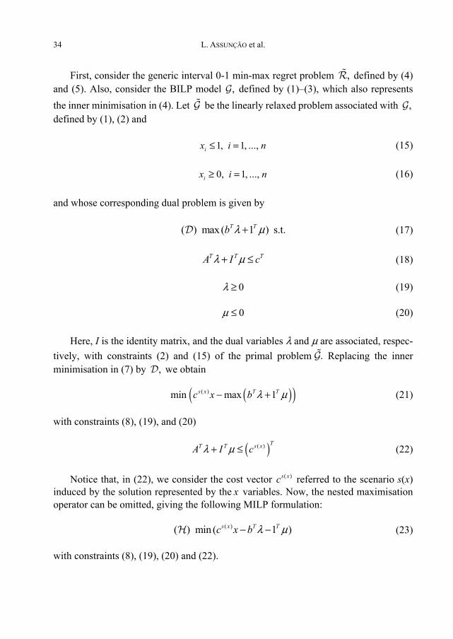
First, consider the generic interval 0-1 min-max regret problem , defined by (4) and (5). Also, consider the BILP model , defined by (1)–(3), which also represents the inner minimisation in (4). Let be the linearly relaxed problem associated with , defined by (1), (2) and

1 1, ., ..,ix i n≤ = (15)

0, 1, ...,ix i n≥ = (16)

and whose corresponding dual problem is given by

( ) max ( 1 ) s.t.T Tb λ μ+ (17)

T T TA I cλ μ+ ≤ (18)

0λ ≥ (19)

0μ ≤ (20)

Here, I is the identity matrix, and the dual variables λ and μ are associated, respec-tively, with constraints (2) and (15) of the primal problem . Replacing the inner minimisation in (7) by , we obtain

( )( )( ) mm x 1in as x T Tc x b λ μ− + (21)

with constraints (8), (19), and (20)

( )( ) TT T s xA I cλ μ+ ≤ (22)

Notice that, in (22), we consider the cost vector ( )s xc referred to the scenario s(x) induced by the solution represented by the x variables. Now, the nested maximisation operator can be omitted, giving the following MILP formulation:

( )( ) min ( 1 )s x T Tc x b λ μ− − (23)

with constraints (8), (19), (20) and (22).


35

Proposition 2 [3]. The cost value referred to as an optimal solution for gives an upper bound on the optimal solution value of , and this bound is tight (optimal) if (i) the restriction matrix A is totally unimodular, and (ii) the column vector b is integral.

LPH consists in solving a corresponding heuristic model , obtaining a solution ˆˆ ˆ( , , )x λ μ . Notice that x̂ also belongs to Ω. Then, the bound referred to ˆˆ ˆ( , , )x λ μ can be

improved by computing the robustness cost (maximum regret) ˆ( )R x of ˆ.x Accordingly, the warm-start procedure HS uses ˆ( )R x as an initial primal bound on the solution of . Since computing ˆ( )R x requires finding an optimal solution ôpt ( ( ))s x for the scenario

ˆ( )s x , this solution is also stored by HS as an initial Benders’ cut. From Proposition 2, whenever the classical counterpart problem can be modelled as

a BILP of the form of , with a unimodular restriction matrix and b integral, there is a guarantee of optimality at solving . In these cases, LPH (and, therefore, HS) becomes an exact method itself. As a consequence, there is no need to couple it with the logic-based Benders’ algorithms detailed in Section 3. In fact, applying LPH to the interval data min-max regret versions of the polynomially solvable shortest path and assignment problems presented, respectively, in [20, 21], leads to the same compact MILP formulations proposed and computationally tested in these works. Therefore, HS is specially intended to tackle interval 0-1 robust-hard problems, whose classical counterparts cannot be easily modelled utilizing LP (unless P equals NP).

4.3. Extended heuristic start (extended HS)

The third procedure, called extended heuristic start (extended HS), adapts LPH to retrieve information that can provide additional Benders’ cuts in the same way as in extended Benders’. Such procedure can be seen as an extension of HS and is described in Algorithm 1. First, the heuristic model is solved, obtaining a solution

ˆˆ ˆ( , , ),x λ μ with ˆ .x Ω∈ In addition, all the incumbent solution vectors x Ω∈ found along the process are stored in a set ,Π initially empty. The robustness cost ˆ( )R xreferred to x̂ is then computed by finding an optimal solution ôpt( ( ))s x for the scenario ˆ( )s x induced by x̂ (Step 1, Algorithm 1).

Now, let be the set of the Benders’ cuts obtained by the procedure. Also, let ub∗

keep the smallest robustness cost found so far. At this point of the execution,ôpt( ( ))s x← and ˆ( ).ub R x∗ ← For each ,x Π∈ an optimal solution opt( ( ))s x for

the scenario induced by x is found and added to . In addition, the robustness costs referred to the solutions in Π are computed and used to update ub∗ (see Step 2, Algorithm 1). By the end of the execution of Algorithm 1, ub∗ and keep, respectively,


36

the primal bound and the Benders’ cuts to be initially given to the logic-based Benders’ algorithms discussed in Section 3.

Algorithm 1. Extended HS Input: Cost intervals [ ],i il u referred to , 1, ..., ,ix i n= and the feasible region. Output: ( )* ,, ub where is the set of available Benders’ cuts, and *ub is the smallest

robustness cost found. Π ← ∅ Step I. Heuristic initialisation Solve the heuristic problem obtaining a solution ˆ ,x Ω∈ and store in Π all the

incumbent solution vectors x Ω∈ found along the process; Find an optimal solution ˆopt( ( ))s x for the scenario ˆ( )s x induced by ˆ,x and com-

pute ˆ( ),R x the robustness cost of x̂ ; Step II. Additional cuts generation

( )( ){ }ˆopt ;s x←

( )* ˆ ;ub R x← for all x Π∈ do Find an optimal solution ( )( )opt s x for the scenario induced by x and compute

( ) ,R x the robustness cost of ;x

( )( ){ }opt ;s x← ∪

( ){ }* * min , ;ub ub R x← end return ( )* ., ub

5. Case studies in solving interval 0-1 robust-hard problems

In this section, we evaluate the impact of the warm-start procedures discussed in Section 4 on the quality of the solutions obtained by standard Benders’ and extended Benders’ while solving two interval 0-1 robust-hard problems, namely the restricted robust shortest path problem (R-RSP) [3] and the robust set covering problem (RSC) [34]. They consist of interval data min-max regret versions of the restricted shortest path problem (R-SP) [18], and the Set Covering problem (SC) [18], respectively.

We computationally compare a total of six algorithms obtained from coupling these logic-based Benders’ algorithms with the warm-start procedures in different manners,


37

as detailed in Table 1. To limit the number of combinations tested, HS is only used as warm start for standard Benders’, while extended HS is only applied for extended Benders’.

Table 1. Algorithms obtained from coupling standard Benders’ and extended Benders’ with the warm-start procedures

Algorithm Benders’ algorithm Warm-start Standard Extended RS HS Extended HS

RS Benders’ × × HS Benders’ × × RS-HS Benders’ × × × Extended RS Benders’ × × Extended HS Benders’ × × Extended RS-HS Benders’ × × ×

The computational experiments were performed on a 64 bits Intel Xeon E5405

machine with 2.0 GHz and 7.0 GB of RAM, under Linux operating system. The algorithms were developed in C++, and each logic-based Benders’ algorithm was set to run for up to 3600. ILOG CPLEX1 12.5 under default parameters was used to solve their master problems, as well as to address the corresponding ILP formulations for the classical R-SP and SC (as described in [3, 34]), since the solver alone is competitive in solving these problems [9, 38]. We also used CPLEX to tackle the corresponding heuristic formulations related to LPH.

Two experiments are performed for both R-RSP and RSC. The goal of the first one is to compare the results produced by standard Benders’ and extended Benders’, while the second evaluates the impact of the warm-start procedures. All the times considered and reported in our experiments correspond to wall-clock time.

5.1. The restricted robust shortest path problem (R-RSP)

R-RSP is an interval data min-max regret version of the Restricted Shortest Path problem (R-SP), an extensively studied NP-hard problem [18]. Consider a digraph

( , ),G V A= where V is the set of vertices, and A is the set of arcs. With each arc(i, j) ∈ A, we associate a resource consumption ijd +∈ and a continuous cost interval ,[ , ]ij ijl u where ijl +∈ is the lower bound, and iju +∈ is the upper bound on this interval of cost, with .ij ijl u≤ An origin vertex o V∈ and a destination one t V∈ are also given, as well as a value ,β ∈ parameter used to limit the resource consumed along a path fromo to t in G .

_________________________ 1https://www.ibm.com/analytics/cplex-optimizer


38

Here, a scenario s is an assignment of arc costs, where a cost [ , ]sij ij ijc l u∈ is fixed

for all (i, j) ∈ A. Let be the set of all paths from o to t and [ ]A p be the set of the arcs that compose a path .p ∈ Also let be the set of all possible cost scenarios of G. The cost of a path p ∈ in a scenario s∈ is given by

( , ) [ ].s s

p iji j A p

C c∈

= Similarly, the

resource consumption referred to a path p ∈ is given by ( , ) [ ]

.p iji j A p

D d∈

= Also

consider { }( ,|) pp Dβ β= ∈ ≤ the subset of paths in whose resource con-

sumptions are smaller than or equal to β. Considering the definitions in Section 3.1, R-RSP aims at finding a robust solution

path among the ones in ( ).Ω β=

Implementation details. For the logic-based Benders’ decomposition, we consider the mathematical formulation proposed in [3], which follows the standard modelling technique described in Section 3.1. Likewise, the relaxed formulation solved by LPH and the one used to model the R-SP, the classical optimisation counterpart, are the same as adopted in [3].

Benchmark instances. In our experiments, we use two benchmarks of R-RSP instances adapted from the literature of the robust shortest path problem [20]: Karaşan [20], and Coco [10] instances, which simulate, respectively, telecommunications and urban transportation networks. The resulting R-RSP benchmarks are introduced in [3].

Karaşan instances consist of layered [36] and acyclic [8] digraphs. In these digraphs, each of the κ layers has the same number ω of vertices. There is an arc from every vertex in a layer { }1, ..., 1b κ∈ − to every vertex in the adjacent layer 1.b + Moreover, there is an arc from the origin o to every vertex in the first layer, and an arc from every vertex in the layer κ to the destination vertex t. These instances are named K-v-Φmax-δ-ω, where v is the number of vertices (aside from o and t), Φmax is an integer constant, and 0 1δ< < is a continuous value. The arc cost intervals are generated as follows. For each arc ( , ) ,i j A∈ a random integer value ijΦ is uniformly chosen in the range max[1, ].ΦAfterwards, random integer values ijl and iju are uniformly selected, respectively, in the ranges [(1 ) , (1 ) ]ij ijδ Φ δ Φ− + and [ , (1 ) ].ij ijl δ Φ+ Note that Φ plays the role of a base-case scenario, and δ determines the degree of uncertainty.

Coco’s instances consist of grid digraphs based on n m× matrices, where n is the number of rows and m is the number of columns. Each matrix cell corresponds to a vertex in the digraph, and there are two bidirectional arcs between each pair of vertices whose respective matrix cells are adjacent. The origin 𝑜 is defined as the upper left vertex, and the destination t is defined as the lower right vertex. These instances are


39

named G-n×m-Φmax-δ, with 0 1,δ< < where Φmax is an integer value. Given Φmax and δ values, the cost intervals are generated as in Karaşan’s instances.

For all instances, the resource consumption associated with each arc is given by a random integer value uniformly selected in the interval (0, 10]. As pointed out in [3], the small interval amplitude allows the generation of instances in which most of the arcs are candidates to appear in an optimal solution. The resource consumption limit β of a given instance is computed as follows. Consider the set of all the paths from o to t, and let p ∈ be the shortest path in terms of resource consumption, i.e., .arg min pp

p D∈

=

We

set 1 ,1. pDβ = which means that 10% tolerance is given concerning the minimum resource consumption pD .

In our experiments, we use Karaşan’s and Coco’s instances of 1000 and 2000 vertices, with { }max 20, 200 ,Φ ∈ { }0.5,0.9δ ∈ , and { }5,10, 25 .ω ∈ For each possible parameters configuration, we consider a group of 10 instances. In summary, 480 R-RSP instances are used in the experiments.

Computional results. The first experiment is performed to compare the quality of the solutions obtained by standard Benders’ and extended Benders’ for the two benchmarks and, thus, to check if the generation of additional Benders’ cuts as in extended Benders’ leads to better bounds for R-RSP. Results for Karaşan’s and Coco’s instances are reported in Tables 2 and 3, respectively. In both tables, the first column displays the name of each set of 10 instances. For each algorithm, the #opt column displays the number of instances solved at optimality within 3600 s of execution. The average processing time (in s) spent in solving these instances is reported in the next column in a row. If no instance in the set is solved at optimality, this entry is filled with a dash. For each set of instances, it is also reported the average and the standard deviation (over

the 10 instances) of the relative optimality gaps given by100 ,UB LBUB−× where LB and

UB are the best lower and upper bounds, respectively, obtained by the corresponding algorithm within the time limit. The last row shows, for each algorithm, the average of the optimality gaps over all instances considered and the average of the standard deviations referred to each set of instances.

Regarding Karaşan’s instances (Table 2), it can be seen that the average optimality gaps referred to the solutions provided by standard Benders’ are up to 7.47% for the instances with 1000 vertices (see K-1000-20-0.9-5), while those of extended Benders’ are at most 4.25% for the same instances. Moreover, the average optimality gaps referred to the solutions provided by standard Benders’ are up to 25.77% for the instances with 2000 vertices (see K-2000-200-0.9-5), whereas those of extended Benders’ are up to 21.35% for the same instances. In fact, the average gaps of the solutions provided by extended Benders’ are smaller than or equal to those of standard Benders’ for all sets of


40

instances. In addition, extended Benders’ was able to solve at optimality eleven more instances than standard Benders’ (two from K-1000-20-0.5-5, three from K-1000-200- -0.9-5, five from K-2000-200-0.5-10 and one from K-2000-200-0.9-10).

With respect to Coco’s instances (Table 3), the average optimality gaps obtained by standard Benders’ are up to 11.50% (see G-5×400-200-0.9), while those of extended Ben- ders’ are at most 7.18% for the same instances. The average optimality gap of standard Benders’ over all Coco’s instances is very small (1.15%), while that of extended Benders’ is even tighter (0.58%). Once again, the average relative gaps referred to the solutions provided by Extended Benders are smaller than or equal to those of standard Benders’ for all sets of instances. Moreover, extended Benders’ was able to solve at optimality thirteen more instances than standard Benders’, most of them from the sets of hardest instances (5×400 grids).

Table 2. Computational results of standard Benders’ and extended Benders’ for Karaşan’s instances

Test set Standard Benders’ Extended Benders’

#opt Time [s]

GAP [%] Avg

GAP [%] StDev #opt Time

[s] GAP [%]

Avg GAP [%]

StDev K-1000-20-0.5-5 8 1515.25 0.11 0.24 10 1188.80 0.00 0.00 K-1000-20-0.9-5 2 2108.61 7.47 5.29 2 1036.06 4.25 3.74 K-1000-200-0.5-5 10 1165.08 0.00 0.00 10 610.83 0.00 0.00 K-1000-200-0.9-5 1 1919.16 4.85 3.30 4 1658.26 1.78 2.28 K-1000-20-0.5-10 10 83.30 0.00 0.00 10 135.25 0.00 0.00 K-1000-20-0.9-10 10 218.69 0.00 0.00 10 220.23 0.00 0.00 K-1000-200-0.5-10 10 42.54 0.00 0.00 10 119.52 0.00 0.00 K-1000-200-0.9-10 10 413.43 0.00 0.00 10 350.08 0.00 0.00 K-1000-20-0.5-25 10 17.61 0.00 0.00 10 32.93 0.00 0.00 K-1000-20-0.9-25 10 32.22 0.00 0.00 10 58.10 0.00 0.00 K-1000-200-0.5-25 10 18.17 0.00 0.00 10 39.56 0.00 0.00 K-1000-200-0.9-25 10 41.04 0.00 0.00 10 79.03 0.00 0.00 K-2000-20-0.5-5 0 – 14.47 5.89 0 – 10.15 5.02 K-2000-20-0.9-5 0 – 25.01 2.69 0 – 20.02 2.64 K-2000-200-0.5-5 0 – 14.45 3.10 0 – 11.32 2.73 K-2000-200-0.9-5 0 – 25.77 3.39 0 – 21.35 3.68 K-2000-20-0.5-10 8 1297.89 0.91 2.23 8 1213.23 0.56 1.43 K-2000-20-0.9-10 0 – 7.34 4.06 0 – 4.36 4.14 K-2000-200-0.5-10 4 846.44 1.37 2.30 9 2312.38 0.37 1.18 K-2000-200-0.9-10 0 – 5.99 2.44 1 3420.52 2.96 2.35 K-2000-20-0.5-25 10 155.30 0.00 0.00 10 236.72 0.00 0.00 K-2000-20-0.9-25 10 408.79 0.00 0.00 10 460.29 0.00 0.00 K-2000-200-0.5-25 10 138.88 0.00 0.00 10 307.21 0.00 0.00 K-2000-200-0.9-25 10 572.74 0.00 0.00 10 651.75 0.00 0.00 Average 4.49 1.46 3.21 1.22


41

The results suggest that the generation of additional Benders’ cuts referred to in-

cumbent solutions (as in extended Benders’) improves the overall quality of the bounds obtained for both benchmarks. Then, a second experiment is performed to evaluate the impact of the warm-start procedures discussed in Section 4 on the quality of the solutions obtained by Standard Benders’ and extended Benders’.

Table 3. Computational results of standard Benders’ and extended Benders’ for Coco’s instances

Test set Standard Benders’ Extended Benders’

#opt Time [s]

GAP [%] Avg


[s] GAP [%]

Avg GAP [%]

StDev G-32×32-20-0.5 10 7.31 0.00 0.00 10 19.86 0.00 0.00 G-32×32-20-0.9 10 8.63 0.00 0.00 10 27.83 0.00 0.00 G-32×32-200-0.5 10 6.83 0.00 0.00 10 22.99 0.00 0.00 G-32×32-200-0.9 10 9.79 0.00 0.00 10 31.92 0.00 0.00 G-20×50-20-0.5 10 6.66 0.00 0.00 10 14.50 0.00 0.00 G-20×50-20-0.9 10 9.14 0.00 0.00 10 26.09 0.00 0.00 G-20×50-200-0.5 10 6.23 0.00 0.00 10 27.88 0.00 0.00 G-20×50-200-0.9 10 13.43 0.00 0.00 10 44.63 0.00 0.00 G-5×200-20-0.5 10 397.06 0.00 0.00 10 246.95 0.00 0.00 G-5×200-20-0.9 9 670.84 0.28 0.89 10 633.04 0.00 0.00 G-5×200-200-0.5 10 153.69 0.00 0.00 10 153.73 0.00 0.00 G-5×200-200-0.9 8 1059.09 0.20 0.50 10 572.84 0.00 0.00 G-44×44-20-0.5 10 23.52 0.00 0.00 10 69.15 0.00 0.00 G-44×44-20-0.9 10 29.43 0.00 0.00 10 107.79 0.00 0.00 G-44×44-200-0.5 10 23.00 0.00 0.00 10 89.61 0.00 0.00 G-44×44-200-0.9 10 38.13 0.00 0.00 10 133.68 0.00 0.00 G-20×100-20-0.5 10 34.77 0.00 0.00 10 102.64 0.00 0.00 G-20×100-20-0.9 10 90.28 0.00 0.00 10 199.45 0.00 0.00 G-20×100-200-0.5 10 47.27 0.00 0.00 10 159.29 0.00 0.00 G-20×100-200-0.9 10 59.16 0.00 0.00 10 180.63 0.00 0.00 G-5×400-20-0.5 1 3444.71 2.57 1.98 7 2562.42 0.57 1.00 G-5×400-20-0.9 0 – 7.76 3.95 1 2659.83 3.94 2.71 G-5×400-200-0.5 1 2719.17 5.24 4.32 4 2063.25 2.17 2.62 G-5×400-200-0.9 0 – 11.50 3.45 0 – 7.18 3.34 Average 1.15 0.63 0.58 0.40

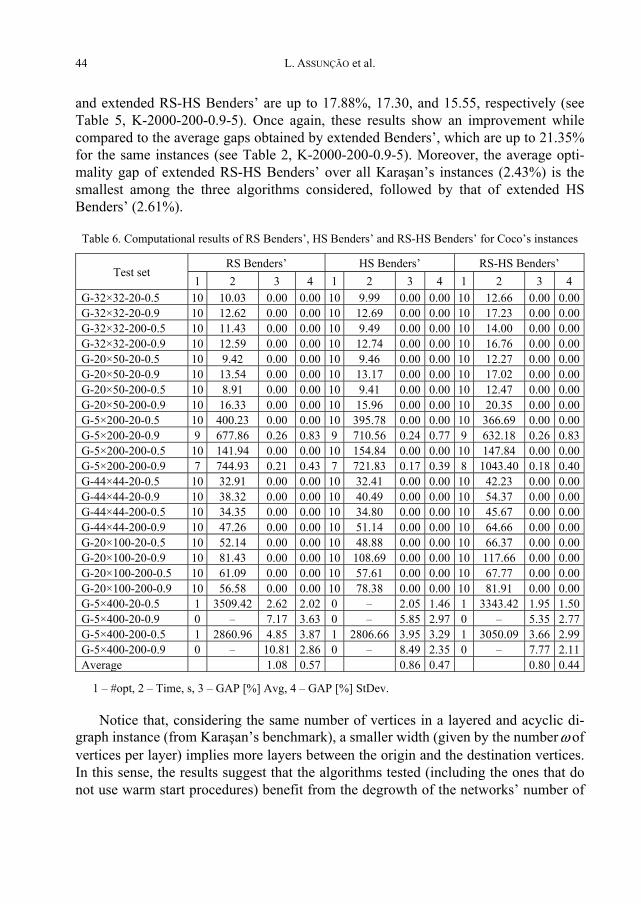
Tables 4 and 6 display the results concerning the first three algorithms in Table 1, the

ones that couple the warm-start procedures with standard Benders’. Tables 5 and 7 show the results concerning the last three algorithms in Table 1, which couple the warm-start proce-dures with extended Benders’. In the tables, the first column displays the name of each set


42

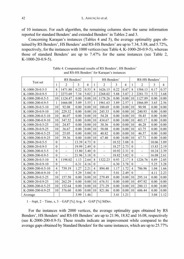
of 10 instances. For each algorithm, the remaining columns show the same information reported for standard Benders’ and extended Benders’ in Tables 2 and 3.

Concerning Karaşan’s instances (Tables 4 and 5), the average optimality gaps obtained by RS Benders’, HS Benders’ and RS-HS Benders’ are up to 7.34, 5.88, and 5.72%, respectively, for the instances with 1000 vertices (see Table 4, K-1000-20-0.9-5), whereas those of standard Benders’ are up to 7.47% for the same instances (see Table 2, K-1000-20-0.9-5).

Table 4. Computational results of RS Benders’, HS Benders’ and RS-HS Benders’ for Karaşan’s instances

Test set RS Benders’ HS Benders’ RS-HS Benders’

1 2 3 4 1 2 3 4 1 2 3 4 K-1000-20-0.5-5 8 1471.80 0.22 0.53 8 1626.15 0.22 0.47 8 1584.13 0.17 0.37 K-1000-20-0.9-5 2 2273.69 7.34 5.02 2 2268.02 5.88 3.87 2 2281.73 5.72 3.68 K-1000-200-0.5-5 10 1124.47 0.00 0.00 10 1178.26 0.00 0.00 10 1127.89 0.00 0.00 K-1000-200-0.9-5 1 1666.08 5.09 3.55 1 1961.63 3.89 2.57 1 1866.89 3.65 2.56 K-1000-20-0.5-10 10 92.08 0.00 0.00 10 100.69 0.00 0.00 10 90.98 0.00 0.00 K-1000-20-0.9-10 10 229.32 0.00 0.00 10 245.33 0.00 0.00 10 240.93 0.00 0.00 K-1000-200-0.5-10 10 46.07 0.00 0.00 10 54.28 0.00 0.00 10 58.45 0.00 0.00 K-1000-200-0.9-10 10 347.52 0.00 0.00 10 434.67 0.00 0.00 10 403.17 0.00 0.00 K-1000-20-0.5-25 10 24.87 0.00 0.00 10 38.36 0.00 0.00 10 46.28 0.00 0.00 K-1000-20-0.9-25 10 36.67 0.00 0.00 10 58.08 0.00 0.00 10 63.75 0.00 0.00 K-1000-200-0.5-25 10 25.05 0.00 0.00 10 40.82 0.00 0.00 10 46.57 0.00 0.00 K-1000-200-0.9-25 10 39.36 0.00 0.00 10 67.40 0.00 0.00 10 67.71 0.00 0.00 K-2000-20-0.5-5 0 – 13.39 4.73 0 – 10.52 3.88 0 – 10.06 3.89 K-2000-20-0.9-5 0 – 19.99 2.49 0 – 18.27 2.73 0 – 15.83 2.19 K-2000-200-0.5-5 0 – 13.80 3.40 0 – 10.92 2.31 0 – 10.24 2.39 K-2000-200-0.9-5 0 – 21.96 3.18 0 – 18.82 3.02 0 – 16.08 2.61 K-2000-20-0.5-10 8 1198.02 1.13 2.64 8 1322.23 0.93 2.17 8 1226.76 0.89 2.05 K-2000-20-0.9-10 0 – 6.31 4.16 0 – 6.30 3.78 0 – 5.25 3.28 K-2000-200-0.5-10 4 739.19 1.27 2.21 4 894.40 1.17 1.72 4 786.96 1.04 1.66 K-2000-200-0.9-10 0 – 5.29 3.04 0 – 5.01 2.49 0 – 4.11 2.23 K-2000-20-0.5-25 10 157.50 0.00 0.00 10 279.49 0.00 0.00 10 295.14 0.00 0.00 K-2000-20-0.9-25 10 262.29 0.00 0.00 10 676.51 0.00 0.00 10 497.92 0.00 0.00 K-2000-200-0.5-25 10 152.64 0.00 0.00 10 271.29 0.00 0.00 10 280.13 0.00 0.00 K-2000-200-0.9-25 10 376.60 0.00 0.00 10 821.86 0.00 0.00 10 606.44 0.00 0.00 Average 3.99 1.46 3.41 1.21 3.04 1.12

1 – #opt, 2 – Time, s, 3 – GAP [%] Avg, 4 – GAP [%] StDev.

For the instances with 2000 vertices, the average optimality gaps obtained by RS Benders’, HS Benders’ and RS-HS Benders’ are up to 21.96, 18.82 and 16.08, respectively (see K-2000-200-0.9-5). These results indicate an improvement while compared to the average gaps obtained by Standard Benders' for the same instances, which are up to 25.77%


43

(see Table 2, K-2000-200-0.9-5). Notice that the average optimality gap of RS-HS Benders’ over all Karaşan’s instances (3.04%) is the smallest among the three algorithms con-sidered, followed by that of HS Benders’ (3.41%). In fact, the average gaps of the solutions provided by RS-HS Benders’ are smaller than or equal to those of the other two algorithms for all sets of Karaşan’s instances.

Table 5. Computational results of extended RS Benders’, extended HS Benders’ and extended RS-HS Benders’ for Karaşan’s instances

Test set Ext. RS Benders’ Ext. HS Benders’ Ext. RS-HS Benders’

1 2 3 4 1 2 3 4 1 2 3 4 K-1000-20-0.5-5 10 1273.60 0.00 0.00 10 1150.63 0.00 0.00 10 1121.10 0.00 0.00 K-1000-20-0.9-5 2 1008.54 4.25 3.56 2 974.51 3.57 2.93 2 973.66 3.61 2.86 K-1000-200-0.5-5 10 585.40 0.00 0.00 10 625.72 0.00 0.00 10 579.66 0.00 0.00 K-1000-200-0.9-5 4 1684.83 1.70 2.24 5 2147.00 1.37 1.66 4 1770.58 1.42 1.74 K-1000-20-0.5-10 10 124.36 0.00 0.00 10 136.95 0.00 0.00 10 133.33 0.00 0.00 K-1000-20-0.9-10 10 196.61 0.00 0.00 10 229.74 0.00 0.00 10 213.50 0.00 0.00 K-1000-200-0.5-10 10 100.70 0.00 0.00 10 136.22 0.00 0.00 10 108.71 0.00 0.00 K-1000-200-0.9-10 10 314.15 0.00 0.00 10 368.19 0.00 0.00 10 336.15 0.00 0.00 K-1000-20-0.5-25 10 30.33 0.00 0.00 10 49.62 0.00 0.00 10 48.45 0.00 0.00 K-1000-20-0.9-25 10 47.25 0.00 0.00 10 77.56 0.00 0.00 10 71.16 0.00 0.00 K-1000-200-0.5-25 10 31.91 0.00 0.00 10 57.52 0.00 0.00 10 54.14 0.00 0.00 K-1000-200-0.9-25 10 55.51 0.00 0.00 10 111.93 0.00 0.00 10 89.35 0.00 0.00 K-2000-20-0.5-5 0 – 9.51 4.54 0 – 8.72 4.05 0 – 8.29 4.02 K-2000-20-0.9-5 0 – 16.97 2.50 0 – 16.48 2.87 0 – 14.94 2.56 K-2000-200-0.5-5 0 – 10.13 3.26 0 – 8.58 2.21 0 – 8.30 2.50 K-2000-200-0.9-5 0 – 17.88 3.09 0 – 17.30 3.28 0 – 15.55 2.60 K-2000-20-0.5-10 8 1128.41 0.55 1.18 8 1253.30 0.48 1.19 8 1211.49 0.53 1.23 K-2000-20-0.9-10 2 3205.89 3.51 3.32 0 – 3.48 2.97 2 3401.90 3.39 3.03 K-2000-200-0.5-10 9 2142.32 0.37 1.18 8 2232.16 0.34 0.96 9 2300.13 0.24 0.76 K-2000-200-0.9-10 1 3408.48 2.44 2.13 1 3291.85 2.35 1.93 1 3108.20 2.05 1.92 K-2000-20-0.5-25 10 232.01 0.00 0.00 10 341.21 0.00 0.00 10 335.37 0.00 0.00 K-2000-20-0.9-25 10 339.85 0.00 0.00 10 687.16 0.00 0.00 10 592.81 0.00 0.00 K-2000-200-0.5-25 10 241.97 0.00 0.00 10 422.96 0.00 0.00 10 362.34 0.00 0.00 K-2000-200-0.9-25 10 471.57 0.00 0.00 10 850.08 0.00 0.00 10 703.65 0.00 0.00 Average 2.80 1.13 2.61 1.00 2.43 0.97


The average optimality gaps referred to the solutions provided by extended RS Benders’, extended HS Benders’ and extended RS-HS Benders’ are up to 4.25, 3.57, and 3.61%, respectively, for the instances with 1000 vertices (see Table 5, K-1000-20- -0.9-5), whereas those of extended Benders’ are up to 4.25% for the same instances (see Table 2, K-1000-20-0.9-5). For the instances with 2000 vertices, the average optimality gaps referred to the solutions provided by extended RS Benders’, extended HS Benders’


44

and extended RS-HS Benders’ are up to 17.88%, 17.30, and 15.55, respectively (see Table 5, K-2000-200-0.9-5). Once again, these results show an improvement while compared to the average gaps obtained by extended Benders’, which are up to 21.35% for the same instances (see Table 2, K-2000-200-0.9-5). Moreover, the average opti-mality gap of extended RS-HS Benders’ over all Karaşan’s instances (2.43%) is the smallest among the three algorithms considered, followed by that of extended HS Benders’ (2.61%).

Table 6. Computational results of RS Benders’, HS Benders’ and RS-HS Benders’ for Coco’s instances

Test set RS Benders’ HS Benders’ RS-HS Benders’

1 2 3 4 1 2 3 4 1 2 3 4 G-32×32-20-0.5 10 10.03 0.00 0.00 10 9.99 0.00 0.00 10 12.66 0.00 0.00 G-32×32-20-0.9 10 12.62 0.00 0.00 10 12.69 0.00 0.00 10 17.23 0.00 0.00 G-32×32-200-0.5 10 11.43 0.00 0.00 10 9.49 0.00 0.00 10 14.00 0.00 0.00 G-32×32-200-0.9 10 12.59 0.00 0.00 10 12.74 0.00 0.00 10 16.76 0.00 0.00 G-20×50-20-0.5 10 9.42 0.00 0.00 10 9.46 0.00 0.00 10 12.27 0.00 0.00 G-20×50-20-0.9 10 13.54 0.00 0.00 10 13.17 0.00 0.00 10 17.02 0.00 0.00 G-20×50-200-0.5 10 8.91 0.00 0.00 10 9.41 0.00 0.00 10 12.47 0.00 0.00 G-20×50-200-0.9 10 16.33 0.00 0.00 10 15.96 0.00 0.00 10 20.35 0.00 0.00 G-5×200-20-0.5 10 400.23 0.00 0.00 10 395.78 0.00 0.00 10 366.69 0.00 0.00 G-5×200-20-0.9 9 677.86 0.26 0.83 9 710.56 0.24 0.77 9 632.18 0.26 0.83 G-5×200-200-0.5 10 141.94 0.00 0.00 10 154.84 0.00 0.00 10 147.84 0.00 0.00 G-5×200-200-0.9 7 744.93 0.21 0.43 7 721.83 0.17 0.39 8 1043.40 0.18 0.40 G-44×44-20-0.5 10 32.91 0.00 0.00 10 32.41 0.00 0.00 10 42.23 0.00 0.00 G-44×44-20-0.9 10 38.32 0.00 0.00 10 40.49 0.00 0.00 10 54.37 0.00 0.00 G-44×44-200-0.5 10 34.35 0.00 0.00 10 34.80 0.00 0.00 10 45.67 0.00 0.00 G-44×44-200-0.9 10 47.26 0.00 0.00 10 51.14 0.00 0.00 10 64.66 0.00 0.00 G-20×100-20-0.5 10 52.14 0.00 0.00 10 48.88 0.00 0.00 10 66.37 0.00 0.00 G-20×100-20-0.9 10 81.43 0.00 0.00 10 108.69 0.00 0.00 10 117.66 0.00 0.00 G-20×100-200-0.5 10 61.09 0.00 0.00 10 57.61 0.00 0.00 10 67.77 0.00 0.00 G-20×100-200-0.9 10 56.58 0.00 0.00 10 78.38 0.00 0.00 10 81.91 0.00 0.00 G-5×400-20-0.5 1 3509.42 2.62 2.02 0 – 2.05 1.46 1 3343.42 1.95 1.50 G-5×400-20-0.9 0 – 7.17 3.63 0 – 5.85 2.97 0 – 5.35 2.77 G-5×400-200-0.5 1 2860.96 4.85 3.87 1 2806.66 3.95 3.29 1 3050.09 3.66 2.99 G-5×400-200-0.9 0 – 10.81 2.86 0 – 8.49 2.35 0 – 7.77 2.11 Average 1.08 0.57 0.86 0.47 0.80 0.44


Notice that, considering the same number of vertices in a layered and acyclic digraph instance (from Karaşan’s benchmark), a smaller width (given by the numberω of vertices per layer) implies more layers between the origin and the destination vertices. In this sense, the results suggest that the algorithms tested (including the ones that do not use warm start procedures) benefit from the degrowth of the networks’ number of


45

layers. Instances generated under ω = 5 (especially the ones with 2000 vertices) are the hardest ones (among Karaşan’s instances) for all algorithms.

For the hardest Karaşan’s instances, the results also suggest that networks generated under a higherδ value (in particular, δ = 0.9) tend to become even more difficult to be solved by any of the exact algorithms tested. A possible explanation for this behaviour is that higher δ values might increase the occurrence of overlapping cost intervals, as pointed out in other RO studies in which the uncertainty is generated in a similar manner [20, 34]. From the results, it is not clear how the variation of Φmax (the parameter used to define the case base scenarioΦ, from which the uncertainty is generated) interferes with the performance of the algorithms analysed.

Table 7. Computational results of extended RS Benders’, extended HS Benders’ and extended RS-HS Benders’ for Coco’s instances

Test set Ext. RS Benders’ Ext. HS Benders’ Ext. RS-HS Benders’

1 2 3 4 1 2 3 4 1 2 3 4 G-32×32-20-0.5 10 17.57 0.00 0.00 10 21.96 0.00 0.00 10 20.57 0.00 0.00 G-32×32-20-0.9 10 23.93 0.00 0.00 10 26.89 0.00 0.00 10 24.79 0.00 0.00 G-32×32-200-0.5 10 20.69 0.00 0.00 10 24.12 0.00 0.00 10 22.45 0.00 0.00 G-32×32-200-0.9 10 28.01 0.00 0.00 10 32.02 0.00 0.00 10 29.74 0.00 0.00 G-20×50-20-0.5 10 14.38 0.00 0.00 10 16.69 0.00 0.00 10 16.76 0.00 0.00 G-20×50-20-0.9 10 24.68 0.00 0.00 10 33.47 0.00 0.00 10 28.01 0.00 0.00 G-20×50-200-0.5 10 20.03 0.00 0.00 10 26.17 0.00 0.00 10 23.91 0.00 0.00 G-20×50-200-0.9 10 34.80 0.00 0.00 10 41.58 0.00 0.00 10 35.84 0.00 0.00 G-5×200-20-0.5 10 253.82 0.00 0.00 10 270.67 0.00 0.00 10 252.15 0.00 0.00 G-5×200-20-0.9 10 625.29 0.00 0.00 10 674.93 0.00 0.00 10 662.37 0.00 0.00 G-5×200-200-0.5 10 137.56 0.00 0.00 10 162.04 0.00 0.00 10 145.38 0.00 0.00 G-5×200-200-0.9 10 596.76 0.00 0.00 10 613.23 0.00 0.00 10 572.16 0.00 0.00 G-44×44-20-0.5 10 58.12 0.00 0.00 10 79.05 0.00 0.00 10 67.88 0.00 0.00 G-44×44-20-0.9 10 87.62 0.00 0.00 10 115.30 0.00 0.00 10 94.41 0.00 0.00 G-44×44-200-0.5 10 77.54 0.00 0.00 10 100.56 0.00 0.00 10 84.27 0.00 0.00 G-44×44-200-0.9 10 112.27 0.00 0.00 10 140.27 0.00 0.00 10 125.03 0.00 0.00 G-20×100-20-0.5 10 96.62 0.00 0.00 10 115.32 0.00 0.00 10 109.56 0.00 0.00 G-20×100-20-0.9 10 159.73 0.00 0.00 10 219.97 0.00 0.00 10 189.91 0.00 0.00 G-20×100-200-0.5 10 144.09 0.00 0.00 10 167.32 0.00 0.00 10 147.89 0.00 0.00 G-20×100-200-0.9 10 139.18 0.00 0.00 10 202.99 0.00 0.00 10 165.75 0.00 0.00 G-5×400-20-0.5 7 2544.20 0.54 1.01 7 2488.07 0.42 0.74 7 2572.86 0.34 0.64 G-5×400-20-0.9 1 2504.97 4.04 3.10 1 2394.92 3.12 2.25 1 2315.17 2.95 2.18 G-5×400-200-0.5 4 1992.37 2.18 2.32 4 2016.87 1.72 1.95 4 1998.41 1.70 1.91 G-5×400-200-0.9 0 – 6.83 2.75 0 – 5.27 2.10 0 – 5.11 2.11 Average 0.57 0.38 0.44 0.29 0.42 0.28



46

Regarding Coco’s instances (Tables 6 and 7), the average optimality gaps obtained by RS Benders’, HS Benders’, and RS-HS Benders’ are up to 10.81, 8.49, and 7.77%, respectively (see Table 6, G-5×400-200-0.9). Recall that the average optimality gaps obtained by standard Benders’ are up to 11.50% for the same instances (see Table 3, G-5×400-200-0.9). The average optimality gap of RS-HS Benders’ over all Coco’s instances (0.80%) is the smallest among the three algorithms considered, followed by that of HS Benders’ (0.86%). In addition, RS-HS Benders’ was always able to provide tighter average optimality gaps for the hardest instances (5×400 grids).

Fig. 1. Summary of the average gaps obtained for the hardest Karaşan’s instances;

upper: instance set K-1000-20-0.9-5, lower: instance set K-2000-200-0.9-5


47

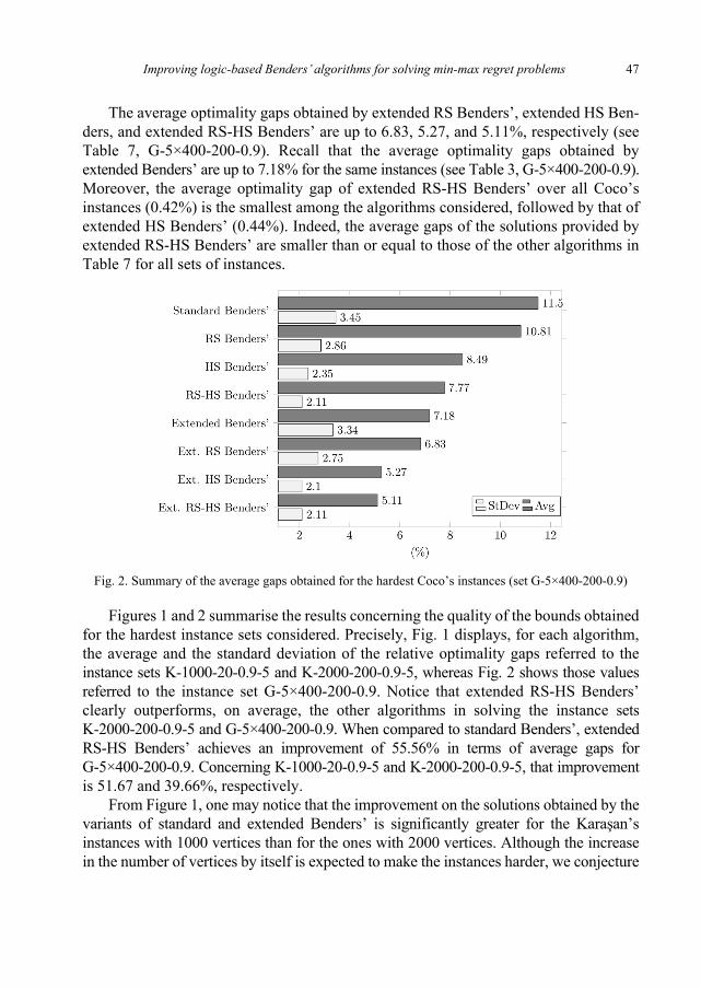
The average optimality gaps obtained by extended RS Benders’, extended HS Ben- ders, and extended RS-HS Benders’ are up to 6.83, 5.27, and 5.11%, respectively (see Table 7, G-5×400-200-0.9). Recall that the average optimality gaps obtained by extended Benders’ are up to 7.18% for the same instances (see Table 3, G-5×400-200-0.9). Moreover, the average optimality gap of extended RS-HS Benders’ over all Coco’s instances (0.42%) is the smallest among the algorithms considered, followed by that of extended HS Benders’ (0.44%). Indeed, the average gaps of the solutions provided by extended RS-HS Benders’ are smaller than or equal to those of the other algorithms in Table 7 for all sets of instances.

Fig. 2. Summary of the average gaps obtained for the hardest Coco’s instances (set G-5×400-200-0.9)

Figures 1 and 2 summarise the results concerning the quality of the bounds obtained for the hardest instance sets considered. Precisely, Fig. 1 displays, for each algorithm, the average and the standard deviation of the relative optimality gaps referred to the instance sets K-1000-20-0.9-5 and K-2000-200-0.9-5, whereas Fig. 2 shows those values referred to the instance set G-5×400-200-0.9. Notice that extended RS-HS Benders’ clearly outperforms, on average, the other algorithms in solving the instance sets K-2000-200-0.9-5 and G-5×400-200-0.9. When compared to standard Benders’, extended RS-HS Benders’ achieves an improvement of 55.56% in terms of average gaps for G-5×400-200-0.9. Concerning K-1000-20-0.9-5 and K-2000-200-0.9-5, that improvement is 51.67 and 39.66%, respectively.

From Figure 1, one may notice that the improvement on the solutions obtained by the variants of standard and extended Benders’ is significantly greater for the Karaşan’s instances with 1000 vertices than for the ones with 2000 vertices. Although the increase in the number of vertices by itself is expected to make the instances harder, we conjecture


48

that, once again, the topology of these instances can contribute to this behaviour. As already mentioned, for the same number of vertices, the difficulty of Karaşan’s instances tends to grow with the increase in the number of layers. In particular, for the two instance sets highlighted, the number of vertices in each layer is the same (ω = 5) and, thus, K-2000-200-0.9-5 instances not only have the double of the vertices of K-1000-20-0.9-5, but also the double of layers.

5.2. The robust set covering problem (RSC)

RSC is an interval data min-max regret generalisation of the strongly NP-hard set covering problem (SC) [18]. Let { }ijO o= be an i j× binary matrix such that { }1, ...,I i=

and { }1, ...,J j= are its corresponding row and column sets, respectively. We say that a column j J∈ covers a row i I∈ if 1ijo = . In this sense, a covering is a subset K J⊆ of columns such that every row in I is covered by at least one column from .K Hereafter, we denote by Λ the set of all possible coverings.

In the case of RSC, a continuous cost interval [ , ]j jl u is associated with each column ,j J∈ with ,j jl u +∈ and .j jl u≤ Accordingly, a scenario s is an assignment of

column costs, where a cost [ , ]sj j jc l u∈ is fixed for all .j J∈ The set of all these

possible cost scenarios is denoted by , and the cost of a covering K Λ∈ in a scenarios∈ is given by .s s

K jj K

C c∈

=

Considering the definitions in Section 3.1, RSC aims at finding a robust solution covering among the ones in .Ω Λ=

Implementation details. For the logic-based Benders’ decomposition and the classical SC, we consider the same mathematical formulations used in [34].

Benchmark instances. For the relaxed formulation solved by LPH, we refer to [3]. In our experiments, we consider three benchmarks of instances from the literature of RSC, namely Beasley’s, Montemanni’s and Kasperski-Zieliński’s benchmarks [34]. The three of them are based on classical SC instances from the OR-library [6]. However, the way the column cost intervals are generated differs from benchmark to benchmark.

Regarding Beasley’s instances, let jΦ represent the cost of a column j J∈ in the original SC instance, and let 0 1δ< < be a continuous value used to control the level of uncertainty referred to an RSC instance. For each ,j J∈ the corresponding cost interval[ , ]j jl u is generated by uniformly selecting random integer values jl and ju in the ranges [(1 ) , ]j jδ Φ Φ− and [ , (1 ) ],j jΦ δ Φ+ respectively. These instances are named


49

B <SCins> –δ, where <SCins> stands for the name of the original SC instance set considered. For each original instance of the classical SC, we consider three RSC instances, one for each value { }0.1, 0.3, 0.5 .δ ∈ In total, 75 instances from Beasley’s benchmark are used in our experiments.

In Montemanni’s instances, the column costs of the original SC instances are discarded, and, for each column ,j J∈ the corresponding cost interval [ , ]j il u is generated as follows. First, a random integer value ju is uniformly chosen in the range [0, 1000], and, then, a random integer value jl is uniformly selected in the range [0, ].ju These instances are named M <SCinst> –1000, where <SCinst> is the name of the original SC instance set used. Each original SC instance considered gives the backbone to generate three RSC instances, and a total of 75 instances from Montemanni’s benchmark are used in our experiments.

Kasperski–Zieliński’s benchmark also considers classical SC instances without the original column costs. In these instances, the cost interval [ , ]j il u of each column j J∈ is generated as follows. First, a random integer value jl is uniformly chosen in the range [0,1000]. Then, a random integer value ju s uniformly selected in the range [ , 1000].j jl l + These instances are named KZ <SCinst> –1000, where <SCinst> is the name of the original SC instance set used. Each of the SC instances considered gives the backbone to generate three RSC instances, and a total of 75 instances from Kasperski–Zieliński’s benchmark are used in our experiments. In summary, 225 RSC instances are considered in the experiments.

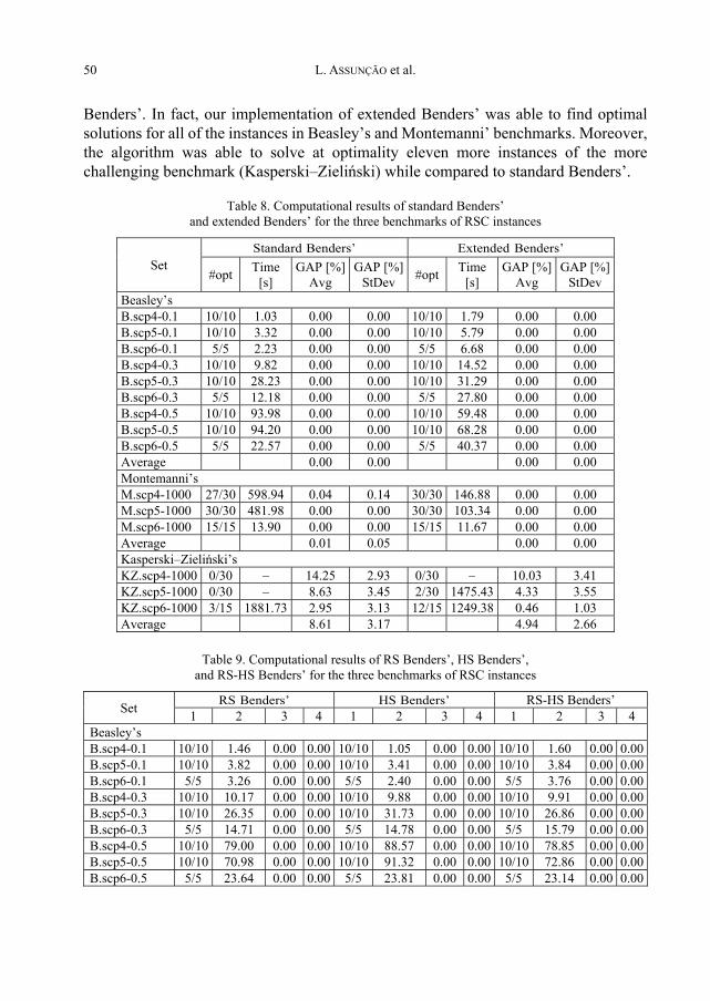
Computational results. First, we reproduced the experiments of [34] to evaluate the performance of standard Benders’ and extended Benders’ in solving RSC instances. Table 8 gives a detailed report of the results obtained for the three benchmarks of instances considered. The first column displays the name of each instance set. For each algorithm, the #opt column gives (i) the number of instances solved at optimality within 3600 s, over (ii) the cardinality of the corresponding instance set. The average processing time (in s) spent in solving these instances is reported in the next column in a row. If no instance in the set is solved at optimality, this entry is filled with a dash. For each set of instances, the average and the standard deviation of the relative optima-

lity gaps given by 100 UB LBUB−× is also reported. Recall that LB and UB are the best

lower and upper bounds, respectively, obtained by the corresponding algorithm within the time limit. The last row shows, for each algorithm and benchmark, the average of the optimality gaps over all instances considered and the average of the standard deviations referred to each set of instances.

Our results agree with the ones presented in [34] and indicate that generating additional cuts as in extended Benders’ improves the bounds obtained by standard


50

Benders’. In fact, our implementation of extended Benders’ was able to find optimal solutions for all of the instances in Beasley’s and Montemanni’ benchmarks. Moreover, the algorithm was able to solve at optimality eleven more instances of the more challenging benchmark (Kasperski–Zieliński) while compared to standard Benders’.

Table 8. Computational results of standard Benders’ and extended Benders’ for the three benchmarks of RSC instances

Set Standard Benders’ Extended Benders’

#opt Time [s]

GAP [%] Avg


[s] GAP [%]

Avg GAP [%]

StDev Beasley’s B.scp4-0.1 10/10 1.03 0.00 0.00 10/10 1.79 0.00 0.00 B.scp5-0.1 10/10 3.32 0.00 0.00 10/10 5.79 0.00 0.00 B.scp6-0.1 5/5 2.23 0.00 0.00 5/5 6.68 0.00 0.00 B.scp4-0.3 10/10 9.82 0.00 0.00 10/10 14.52 0.00 0.00 B.scp5-0.3 10/10 28.23 0.00 0.00 10/10 31.29 0.00 0.00 B.scp6-0.3 5/5 12.18 0.00 0.00 5/5 27.80 0.00 0.00 B.scp4-0.5 10/10 93.98 0.00 0.00 10/10 59.48 0.00 0.00 B.scp5-0.5 10/10 94.20 0.00 0.00 10/10 68.28 0.00 0.00 B.scp6-0.5 5/5 22.57 0.00 0.00 5/5 40.37 0.00 0.00 Average 0.00 0.00 0.00 0.00 Montemanni’s M.scp4-1000 27/30 598.94 0.04 0.14 30/30 146.88 0.00 0.00 M.scp5-1000 30/30 481.98 0.00 0.00 30/30 103.34 0.00 0.00 M.scp6-1000 15/15 13.90 0.00 0.00 15/15 11.67 0.00 0.00 Average 0.01 0.05 0.00 0.00 Kasperski–Zieliński’s KZ.scp4-1000 0/30 – 14.25 2.93 0/30 – 10.03 3.41 KZ.scp5-1000 0/30 – 8.63 3.45 2/30 1475.43 4.33 3.55 KZ.scp6-1000 3/15 1881.73 2.95 3.13 12/15 1249.38 0.46 1.03 Average 8.61 3.17 4.94 2.66

Table 9. Computational results of RS Benders’, HS Benders’,

and RS-HS Benders’ for the three benchmarks of RSC instances

Set RS Benders’ HS Benders’ RS-HS Benders’ 1 2 3 4 1 2 3 4 1 2 3 4

Beasley’s B.scp4-0.1 10/10 1.46 0.00 0.00 10/10 1.05 0.00 0.00 10/10 1.60 0.00 0.00 B.scp5-0.1 10/10 3.82 0.00 0.00 10/10 3.41 0.00 0.00 10/10 3.84 0.00 0.00 B.scp6-0.1 5/5 3.26 0.00 0.00 5/5 2.40 0.00 0.00 5/5 3.76 0.00 0.00 B.scp4-0.3 10/10 10.17 0.00 0.00 10/10 9.88 0.00 0.00 10/10 9.91 0.00 0.00 B.scp5-0.3 10/10 26.35 0.00 0.00 10/10 31.73 0.00 0.00 10/10 26.86 0.00 0.00 B.scp6-0.3 5/5 14.71 0.00 0.00 5/5 14.78 0.00 0.00 5/5 15.79 0.00 0.00 B.scp4-0.5 10/10 79.00 0.00 0.00 10/10 88.57 0.00 0.00 10/10 78.85 0.00 0.00 B.scp5-0.5 10/10 70.98 0.00 0.00 10/10 91.32 0.00 0.00 10/10 72.86 0.00 0.00 B.scp6-0.5 5/5 23.64 0.00 0.00 5/5 23.81 0.00 0.00 5/5 23.14 0.00 0.00


51

Table 9. Computational results of RS Benders’, HS Benders’, and RS-HS Benders’ for the three benchmarks of RSC instances

Set RS Benders’ HS Benders’ RS-HS Benders’ 1 2 3 4 1 2 3 4 1 2 3 4

Average 0.00 0.00 0.00 0.00 0.00 0.00 Montemanni’s M.scp4-1000 29/30 451.00 0.01 0.05 27/30 542.66 0.03 0.15 29/30 444.40 0.01 0.07 M.scp5-1000 30/30 301.02 0.00 0.00 30/30 430.25 0.00 0.00 30/30 315.78 0.00 0.00 M.scp6-1000 15/15 8.84 0.00 0.00 15/15 12.56 0.00 0.00 15/15 10.05 0.00 0.00 Average 0.00 0.02 0.01 0.05 0.00 0.02 Kasperski–Zieliński’s KZ.scp4-1000 0/30 – 10.80 2.73 0/30 – 12.88 2.82 0/30 – 8.40 2.02 KZ.scp5-1000 0/30 – 5.02 2.07 0/30 – 7.93 2.98 0/30 – 4.02 1.80 KZ.scp6-1000 8/15 1854.59 1.45 2.00 5/15 2337.26 2.84 3.10 7/15 1791.68 1.50 1.79 Average 5.76 2.27 7.88 2.97 4.64 1.87


Table 10. Computational results of extended RS Benders’, extended HS Benders’ and extended RS-HS Benders’ for the three benchmarks of RSC instances

Set Ext. RS Benders’ Ext. HS Benders’ Ext. RS-HS Benders’ 1 2 3 4 1 2 3 4 1 2 3 4

Beasley’s B.scp4-0.1 10/10 2.13 0.00 0.00 10/10 1.94 0.00 0.00 10/10 2.09 0.00 0.00 B.scp5-0.1 10/10 5.44 0.00 0.00 10/10 5.90 0.00 0.00 10/10 6.59 0.00 0.00 B.scp6-0.1 5/5 5.84 0.00 0.00 5/5 5.41 0.00 0.00 5/5 6.09 0.00 0.00 B.scp4-0.3 10/10 14.39 0.00 0.00 10/10 12.21 0.00 0.00 10/10 13.63 0.00 0.00 B.scp5-0.3 10/10 32.39 0.00 0.00 10/10 32.82 0.00 0.00 10/10 30.39 0.00 0.00 B.scp6-0.3 5/5 24.92 0.00 0.00 5/5 23.59 0.00 0.00 5/5 23.29 0.00 0.00 B.scp4-0.5 10/10 58.54 0.00 0.00 10/10 54.98 0.00 0.00 10/10 56.06 0.00 0.00 B.scp5-0.5 10/10 63.71 0.00 0.00 10/10 62.51 0.00 0.00 10/10 63.11 0.00 0.00 B.scp6-0.5 5/5 38.76 0.00 0.00 5/5 43.85 0.00 0.00 5/5 34.94 0.00 0.00 Average 0.00 0.00 0.00 0.00 0.00 0.00 Montemanni’s M.scp4-1000 30/30 121.87 0.00 0.00 30/30 149.84 0.00 0.00 30/30 124.74 0.00 0.00 M.scp5-1000 30/30 77.22 0.00 0.00 30/30 102.43 0.00 0.00 30/30 84.28 0.00 0.00 M.scp6-1000 15/15 9.65 0.00 0.00 15/15 13.15 0.00 0.00 15/15 11.33 0.00 0.00 Average 0.00 0.00 0.00 0.00 0.00 0.00 Kasperski–Zieliński’s KZ.scp4-1000 0/30 – 8.33 2.68 0/30 – 8.97 3.00 0/30 – 6.86 2.28 KZ.scp5-1000 3/30 2169.55 3.13 2.25 3/30 2190.60 4.00 2.94 3/30 1834.13 2.51 1.80 KZ.scp6-1000 13/15 1314.18 0.34 0.95 11/15 1293.23 0.53 1.31 12/15 1316.68 0.35 0.92 Average 3.94 1.96 4.50 2.42 3.24 1.67



52

As for R-RSP, a second experiment is performed to evaluate the impact of the warm-start procedures discussed in Section 4 on the quality of the solutions obtained by standard Benders’ and extended Benders’. Table 9 displays the results concerning the first three algorithms in Table 1, whereas Table 10 shows the results of the last three algorithms in Table 1. In both tables, the first column displays the name of each instance set. The remaining columns show, for each algorithm and benchmark, the same information reported for standard Benders’ and extended Benders’ in Table 8.

(a) Instance set KZ.scp5-1000 Fig. 3. Summary of the average gaps referred to the solutions

obtained for the instance sets; upper: KZ.scp4-1000, lower: KZ.scp5-1000


53

All the variations of standard Benders’ and extended Benders’ tested were able to find optimal solutions for all Beasley’s instances in comparably average times. Moreover, regarding Montemanni’s instances, the average optimality gaps refer to the solutions provided by all of the algorithms are extremely tight. In fact, all the variations of extended Benders’ can find optimal solutions for all Montemanni’s instances. These results were expected since standard Benders’ and extended Benders’ alone can find optimal or near-optimal bounds for both benchmarks (see Table 8). We also highlight that the use of the warm-start procedures does not imply greater average execution times.

Fig. 4. Summary of the average gaps referred to the solutions

obtained for the instance set KZ.scp6-1000

Concerning the hardest benchmark (Kasperski-Zieliński’s instances), the positive impact of the warm-start procedures is very relevant. The average optimality gaps ob-tained by RS Benders’, HS Benders’ and RS-HS Benders’ are up to, respectively, 10.80%, 12.88%, and 8.40% (see Table 9, KZ.scp4-1000), whereas those of standard Benders’ are up to 14.25% for the same instances (see Table 8, KZ.scp4-1000). In turn, the average optimality gaps regarding the solutions provided by extended RS Benders’, extended HS Benders’ and extended RS-HS Benders’ are at most 8.33, 8.97, and 6.86%, respectively (see Table 10, KZ.scp4-1000), whereas those of extended Benders’ are up to 10.03% for the same instances (see Table 8, KZ.scp4-1000). Notice that the average optimality gap of extended RS-HS Benders’ over all Kasperski–Zieliński’ instances (3.24%) is the smallest among the eight algorithms implemented, followed by that of extended RS Benders’ (3.94%).


54

Figures 3 and 4 summarise the averages and the standard deviations of the relative optimality gaps referred to the instance sets KZ.scp4-1000, KZ.scp5-1000 and KZ.scp6-1000, the hardest ones in the RSC benchmarks considered. Notice that extended RS-HS Benders’ outperforms, on average, the other algorithms in solving the instance sets KZ.scp4-1000 and KZ.scp5-1000. When compared to standard Benders’, extended RS- -HS Benders’ achieved an improvement of 51.86 and 70.91% in terms of average gaps for KZ.scp4-1000 and KZ.scp5-1000, respectively (Fig. 3). Also notice that for the set KZ.scp6-1000 (Fig. 4), the average optimality gap achieved by extended RS Benders’ (0.34%) is the smallest among all the algorithms tested, and this value is almost the same as that of extended RS-HS Benders’ (0.35%).

5.3. Summary of the main conclusions

The results for both problems considered follow a similar pattern. Extended Ben- ders’ achieve, on average, better optimality gaps than standard Benders’ for all sets of R-RSP and RSC instances used in the experiments. This fact indicates that generating Benders’ cuts referred to incumbent solutions (as in extended Benders’) can improve the overall quality of the bounds obtained.

The results also suggest that the initial upper bounds provided by the heuristic LPH play a key role in tightening the average optimality gaps referred to the solutions obtained by the algorithms that use HS and extended HS as warm-start procedures. This behaviour, which is more evident while solving the hardest instances, is following the study of [3], whose computational experiments indicate that LPH can obtain optimal or near-optimal primal bounds, particularly for R-RSP and RSC.

We also notice that coupling RS with HS (or extended HS) leads to better solutions than when considering each warm-start procedure separately. We believe that the promising cuts generated by RS and the ones referred to incumbent solutions (in extended Benders’ and its variations) speed up the increase of the lower bounds while solving each master problem in the logic-based Benders’ algorithms. Moreover, the optimal or near-optimal upper bounds provided by LPH (within HS and extended HS) help closing the optimality gaps. This hypothesis explains why extended RS-HS Benders’ stood out in terms of effectiveness while compared to the other algorithms.

6. Concluding remarks

We generically describe a class of robust optimisation problems, namely interval 0-1 min-max regret problems, employing the logic-based Benders’ decomposition framework, which is known to converge to an optimal solution in a finite number of iterations. We also discuss an extended version of the framework that aims at generating multiple


55

cuts per iteration. In addition, we present three warm-start procedures to accelerate the convergence of the framework, as well as its extended version. The procedures work by providing promising initial cuts and primal bounds through the resolution of a linearly relaxed model (RS procedure) and an LP based heuristic (HS and extended HS procedures).

Extensive computational experiments are performed to evaluate the impact of the proposed warm-start procedures on the convergence of the logic-based Benders’ algorithms while solving two challenging robust optimisation problems, namely the restricted robust shortest path problem (R-RSP), and the robust set covering problem (RSC). In our experiments, the procedures were able to tighten the average optimality gaps of the solutions obtained by the resulting algorithms. New optimality certificates are found, especially for the hardest R-RSP instances. From the results, the algorithm called extended RS-HS Benders’, which combines RS and extended HS with the extended logic-based Benders’ framework, stands out in terms of effectiveness while compared to the other algorithms.

We highlight that R-RSP and RSC belong to a more challenging subclass of interval 0-1 min-max regret problems, namely interval 0-1 robust-hard problems. Since the algorithms evaluated in this study apply to any problem in this subclass, future works may use the proposed warm-start procedures to tackle another interval 0-1 robust-hard problems.

Acknowledgements

This work was partially supported by the Brazilian National Council for Scientific and Technological Development (CNPq), the Foundation for Support of Research of the State of Minas Gerais, Brazil (FAPEMIG), and Coordination for the Improvement of Higher Education Personnel, Brazil (CAPES).

References

[1] AISSI H., BAZGAN C., VANDERPOOTEN D., Approximation of min-max and min-max regret versions of some combinatorial optimization problems, Eur. J. Oper. Res., 2007, 179 (2), 281–290.

[2] AISSI H., BAZGAN C., VANDERPOOTEN D., Min-max and min-max regret versions of combinatorial optimization problems: A survey, Eur. J. Oper. Res., 2009, 197 (2), 427–438.

[3] ASSUNÇÃO L., NORONHA T.F., SANTOS A., ANDRADE R., A linear programming based heuristic framework for min-max regret combinatorial optimization problems with interval costs, Comp. Oper. Res., 2017, 81, 51 – 66.

[4] ASSUNÇÃO L., SANTOS A.C., NORONHA T.F., ANDRADE R., On the finite optimal convergence of logic- -based Benders’ decomposition in solving 0-1 min-max regret optimization problems with interval costs, [In:] R. Cerulli, S. Fujishige, R.A. Mahjoub (Eds.), Combinatorial Optimization, ISCO 2016, Lecture Notes in Computer Science, Springer, 2016, 9849, 1–12.

[5] AVERBAKH I., LEBEDEV V., On the complexity of minmax regret linear programming, Eur. J. Oper. Res., 2005, 160 (1), 227–231.


56

[6] BEASLEY J.E., OR-Library: Distributing test problems by electronic mail, J. Oper. Res. Soc., 1990, 41(11), 1069–1072.

[7] BENDERS J.F., Partitioning procedures for solving mixed-variables programming problems, Num. Math., 1962, 4 (1), 238–252.

[8] BONDY J.A., MURTY U.S.R., Graph Theory with Applications, Elsevier, New York 1976. [9] CAPRARA A., TOTH P., FISCHETTI M., Algorithms for the set covering problem, Ann. Oper. Res., 2000,

98 (1), 353–371. [10] COCO A.A., JÚNIOR J.C.A., NORONHA T.F., SANTOS A.C., An integer linear programming formulation

and heuristics for the minmax relative regret robust shortest path problem, J. Global Opt., 2014, 60 (2), 265–287.

[11] COCO A.A., SANTOS A.C., NORONHA T.F., Scenario-based heuristics with path-relinking for the robust set covering problem, Proc. XI Metaheuristics International Conference, Agadir, Marocco, 2015, 1–8.

[12] CODATO G., FISCHETTI M., Combinatorial Benders’ cuts for mixed-integer linear programming, Oper. Res., 2006, 54 (4), 756–766.

[13] CONDE E., Robust minmax regret combinatorial optimization problems with a resource-dependent uncertainty polyhedron of scenarios, Comp. Oper. Res., 2019, 103, 97–108.

[14] CREMA A., Min-max-min robust (relative) regret combinatorial optimization, Math. Meth. Oper. Res., 2020, 92 (2), 249–283.

[15] FEIZOLLAHI M.J., AVERBAKH I., The robust (minmax regret) quadratic assignment problem with interval flows, INFORMS J. Comp., 2014, 26 (2), 321–335.

[16] FISCHETTI M., LODI A., Local branching, Math. Progr., 2003, 98 (1–3), 23–47. [17] FISCHETTI M., SALVAGNIN D., ZANETTE A., A note on the selection of Benders’ cuts, Math. Progr.,

2010, 124 (1–2), 175–182. [18] GAREY M.R., JOHNSON D.S., Computers and Intractability. A Guide to the Theory of NP-Complete-

ness, W. H. Freeman & Co., New York 1979. [19] HOOKER J., OTTOSSON G., Logic-based Benders decomposition, Math. Progr., 2003, 96 (1), 33–60. [20] KARAŞAN O.E., PINAR M.Ç., YAMAN H., The robust shortest path problem with interval data,

Technical Report, Bilkent University, Ankara 2001. [21] KASPERSKI A., KOBYLAŃSKI P., KULEJ M., ZIELIŃSKI P., Minimizing maximal regret in discrete

optimization problems with interval data, [In:] Issues in Soft Computing. Decisions and Operations Research, O. Hryniewicz, J. Kacprzyk, D. Kuchta (Eds.), Akademicka Oficyna Wydawnicza EXIT, Warszawa 2005.

[22] KASPERSKI A., ZIELIŃSKI P., An approximation algorithm for interval data minmax regret combinatorial optimization problems, Inf. Proc. Lett., 2006, 97 (5), 177–180.

[23] KASPERSKI A., ZIELIŃSKI P., Soft robust solutions to possibilistic optimization problems, Fuzzy Sets Syst., 2020, DOI: 10.1016/j.fss.2020.12.016.

[24] KASPERSKI A., Discrete Optimization with Interval Data. Minmax Regret and Fuzzy Approach (Studies in Fuzziness and Soft Computing), Springer, Berlin 2008.

[25] KOUVELIS P., YU G., Robust Discrete Optimization and Its Applications, Kluwer, Boston 1997. [26] MCDANIEL D., DEVINE M., A modified Benders’ partitioning algorithm for mixed integer program-

ming, Manage. Sci., 1977, 24 (3), 312–319. [27] GOERIGK M., KASPERSKI A., ZIELINSKI P., Combinatorial two-stage minmax regret problems under

interval uncertainty, Ann. Oper. Res., 2020, 1–28. [28] MONTEMANNI R., BARTA J., GAMBARDELLA L.M., Heuristic and preprocessing techniques for the

robust traveling salesman problem with interval data, Technical Report, Dalle Molle Institute for Artificial Intelligence, 2006.

[29] MONTEMANNI R., BARTA J., GAMBARDELLA L.M., The robust traveling salesman problem with interval data, Trans. Sci., 2007, 41 (3), 366–381.


57

[30] MONTEMANNI R., GAMBARDELLA L.M., A branch and bound algorithm for the robust spanning tree problem with interval data, Eur. J. Oper. Res., 2005, 161 (3), 771–779.

[31] MONTEMANNI R., GAMBARDELLA L.M., The robust shortest path problem with interval data via Benders decomposition, 4OR, 2005, 3 (4), 315–328.

[32] MONTEMANNI R., A Benders decomposition approach for the robust spanning tree problem with inter-val data, Eur. J. Oper. Res., 2006, 174 (3), 1479–1490.

[33] PEREIRA J., AVERBAKH I., Exact and heuristic algorithms for the interval data robust assignment problem, Comp. Oper. Res., 2011, 38 (8), 1153–1163.

[34] PEREIRA J., AVERBAKH I., The robust set covering problem with interval data, Ann. Oper. Res., 2013, 207 (1), 217–235.

[35] SPALL J.C., Introduction to Stochastic Search and Optimization. Estimation, Simulation and Control, Wiley, New York 2003.

[36] SUGIYAMA K., TAGAWA S., TODA M., Methods for visual understanding of hierarchical system struc- tures, IEEE Trans. Syst., Man Cyber., 1981, 11 (2), 109–125.

[37] YU G., On the max-min 0-1 knapsack problem with robust optimization applications, Oper. Res., 1996, 44 (2), 407–415.

[38] ZHU X., WILHELM W.E., A three-stage approach for the resource-constrained shortest path as a sub-problem in column generation, Comp. Oper. Res., 2012, 39 (2), 164–178.

IMPROVING LOGIC-BASED BENDERS’ ALGORITHMS FOR …

Documents

Transcript of IMPROVING LOGIC-BASED BENDERS’ ALGORITHMS FOR …