IMPROVING LIQUID CHROMATOGRAPHY PERFORMANCE: NOVEL...

i

IMPROVING LIQUID CHROMATOGRAPHY PERFORMANCE:

NOVEL DEVELOPMENTS IN PRECONCENTRATION,

INSTRUMENTATION AND OPTIMIZATION

by

Stephen R. Groskreutz

B.A. Chemistry ACS, Gustavus Adolphus College, 2012

Submitted to the Graduate Faculty of

The Kenneth P. Dietrich School of Arts and Sciences

in partial fulfillment of the requirements for the degree of

Doctor of Philosophy

University of Pittsburgh

2017

ii

UNIVERSITY OF PITTSBURGH

DIETRICH SCHOOL OF ARTS AND SCIENCES

This dissertation was presented

by

Stephen R. Groskreutz

It was defended on

December 13, 2016

and approved by

Adrian C. Michael, Professor, Department of Chemistry

Rena A. S. Robinson, Assistant Professor, Department of Chemistry

Gert Desmet, Professor, Department of Chemical Engineering and Industrial Chemistry,

Vrije Universiteit Brussel, Belgium

Dissertation Advisor: Stephen G. Weber, Professor, Department of Chemistry

iii

Copyright © by Stephen R. Groskreutz

2017

iv

IMPROVING LIQUD CHROMATOGRAPHY PERFORMANCE:

NOVEL DEVELOPMENTS IN PRECONCENTRATION,

INSTRUMENTATION AND OPTIMIZATION

Stephen R. Groskreutz, PhD

University of Pittsburgh, 2017

Maximizing performance when using real-world samples and small volume, high sensitivity

columns which degrade the native chromatographic separation is a challenge. Loss in column

performance is due to precolumn dispersion and volume overload. In this work a series of methods

based on novel instrumentation and sound theory is presented to improve a chromatographic result

for such samples in both isocratic and gradient elution modes. An approach called temperature-

assisted solute focusing (TASF) was developed to improve sample focusing or preconcentration.

TASF is designed to address precolumn dispersion in capillary scale LC. Volume overload is a

common form of precolumn dispersion and degrades LC performance. TASF works by relying on

the temperature dependence of solute retention and high power thermoelectric or Peltier elements

(TECs) to actively heat/cool a short segment of the column near its inlet during sample loading.

Cooling the head of the column transiently increases retention for solutes during injection,

improving focusing and solving the volume overload problem. Following focusing rapid heating

decreases retention releasing the compressed injection band to the downstream portion of the

column. The TASF approach was assessed using a series of three instruments with well

characterized solutes developing it into a robust platform capable of routine, unattended use. Three

models for solvent-based on-column focusing in isocratic elution were experimentally

v

investigated. Solvent-based on-column focusing is a well-known method to increase concentration

sensitivity and combat precolumn dispersion by injecting samples made in weak elution solvents.

Additionally, solvent-based focusing occurs naturally as a consequence of increased solute

retention in the sample solvent and a step gradient generated by the difference between sample

and mobile phase composition. Finally, a simple graphical method for rapid chromatographic

optimization was developed. This plot was designed specifically to assist practitioners

to determine experimental conditions to achieve a desired column efficiency or peak capacity in

a defined time in both isocratic and gradient elution modes.

vi

TABLE OF CONTENTS

PREFACE ................................................................................................................................ XXX

1.0 INTRODUCTION....................................................................................................................1

1.1 LIQUID CHROMATOGRAPHY ..............................................................................1

1.2 METRICS OF CHROMATOGRPAHIC PERFORMANCE .................................1

1.3 ROLE OF COLUMN DIAMETER IN LC ...............................................................4

1.4 VOLUME OVERLOAD AND ON-COLUMN FOCUSING ...................................7

1.5 IMPACT OF TEMPERATURE ON RETENTION IN LC ...................................10

1.6 SCOPE OF WORK....................................................................................................13

2.0 TEMPERATURE-ASSISTED ON-COLUMN SOLUTE FOCUSING: A GENERAL

METHOD TO REDUCE PRE-COLUMN DISPERSION IN CAPILLARY HIGH

PERFORMANCE LIQUID CHROMATOGRAPHY........................................................15

2.1 INTRODUCTION......................................................................................................15

2.2 THEORY ....................................................................................................................19

2.3 MATERIALS AND METHODS ..............................................................................28

2.3.1 Reagents and solutions ............................................................................28

2.3.2 van`t Hoff retention studies .....................................................................28

2.3.2.1 Instrumentation............................................................................28

2.3.2.2 Chromatographic conditions ......................................................28

2.3.3 TASF instrumentation and chromatographic conditions ....................29

2.3.3.1 Column preparation ....................................................................29

2.3.3.2 TASF instrumentation .................................................................29

vii

2.3.3.3 Injection volume studies ..............................................................31

2.3.3.4 Limit of quantitation study .........................................................31

2.4 RESULTS AND DISCUSSION ................................................................................32

2.4.1 Temperature dependence of solute retention ........................................32

2.4.2 Simulation of TASF chromatograms .....................................................33

2.4.3 Experimental determination of the effect of TASF on peak width .....41

2.4.4 Improvements in concentration detection limit offered by temperature-

assisted solute focusing ............................................................................45

2.5 CONCLUSIONS ........................................................................................................48

3.0 TEMPERATURE-BASED ON-COLUMN SOLUTE FOCUSING IN CAPILLARY

LIQUID CHROMATOGRAPHY REDUCES PEAK BRAODENING FROM

PRECOLUMN DISPERSION AND VOLUME OVERLOAD WHEN USED ALONE

OR WITH SOLVENT-BASED FOCUSING ......................................................................49

3.1 INTRODUCTION......................................................................................................49

3.2 MATERIALS AND METHODS ..............................................................................51

3.2.1 Reagents and solutions ............................................................................51

3.2.2 van`t Hoff retention studies using commercial columns ......................52

3.2.2.1 Chromatographic instrumentation ............................................52

3.2.2.2 Chromatographic conditions ......................................................52

3.2.3 Second generation TASF instrumentation and chromatographic

conditions ..................................................................................................52

3.2.3.1 Column preparation ....................................................................52

3.2.3.2 TASF instrumentation .................................................................53

viii

3.2.3.3 TASF reproducibility study ........................................................56

3.2.3.4 Injection volume study ................................................................56

3.2.3.5 Solvent- and temperature-focusing injection study ..................57

3.2.3.6 TASF applied to increasing the sensitivity for the peptide

galanin ...........................................................................................57


3.3.1 Temperature dependence of retention factors ......................................58

3.3.2 TASF instrumentation .............................................................................58

3.3.3 Effect of TASF on peak width.................................................................62

3.3.4 Combination of solvent- and temperature-based on-column solute

focusing .....................................................................................................62

3.3.5 TASF increases sensitivity for samples made in strong elution

solvent........................................................................................................66

3.4 CONCLUSIONS ........................................................................................................68

4.0 QUANTITATIVE EVALUATION OF MODELS FOR SOLVENT-BASED, ON-

COLUMN FOCUSING IN LIQUID CHROMATOGRAPHY .........................................70

4.1 INTRODUCTION......................................................................................................70

4.2 THEORY ....................................................................................................................73

4.2.1 Derivation of the k2/k1 factor ..................................................................73

4.2.2 The eluted peak width is a robust measure of the on-column focusing

effect ..........................................................................................................78

4.3 INSTRUMENTAITON AND CHROMATOGRAPHIC CONDITIONS .............82

4.3.1 Chemicals ..................................................................................................82

ix

4.3.2 Instrumentation........................................................................................82

4.3.3 Chromatographic conditions ..................................................................84


4.4.1 Accurate determination of solute retention factors ..............................85

4.4.2 System performance evaluation ..............................................................86

4.4.3 Quantitative evaluation of solvent-based focusing................................87

4.4.3.1 Solvent-based on-column focusing examples.............................87

4.4.3.2 Quantitative comparison of focusing models ............................91

4.5 CONCLUSIONS ........................................................................................................95

5.0 TEMPERATURE-ASSISTED SOLUTE FOCUSING WITH SEQUENTIAL

TRAP/RELEASE ZONES IN ISOCRATIC AND GRADIENT CAPILLARY LIQUID

CHROMATOGRAPHY: SIMULATION AND EXPERIMENT .....................................97

5.1 INTRODUCTION......................................................................................................97

5.2 INSTRUMENTATION AND CHROMATOGRAPHIC CONDITIONS ...........100

5.2.1 Chemicals ................................................................................................100

5.2.2 Instrumentation......................................................................................100

5.2.2.1 Solute retention studies..............................................................100

5.2.2.2 Two-stage temperature-assisted solute focusing .....................100

5.2.3 Chromatographic conditions ................................................................103

5.2.3.1 van`t Hoff retention studies .......................................................103

5.2.3.2 Two-stage temperature-assisted solute focusing .....................103

5.2.3.2.1 Column preparation ................................................103

5.2.3.2.2 Two-stage TASF: Isocratic elution .........................104

x

5.2.3.2.3 Two-stage TASF: Gradient elution ........................105

5.3 RESULTS AND DISCUSSION ..............................................................................105

5.3.1 Dependence of retention on temperature and solvent composition ..105

5.3.2 Characterization of two-stage TASF instrument performance .........107

5.3.3 Simulating two-stage temperature-assisted focusing ..........................111

5.3.3.1 Development of simulation procedure .....................................111

5.3.3.2 Simulating two-stage TASF with isocratic elution ..................115

5.3.3.3 Simulating two-stage TASF with solvent gradient elution .....119

5.3.4 Two-stage TASF experiments: Isocratic elution .................................123

5.3.5 Two-stage TASF experiments: Gradient elution ................................127

5.3.6 Assessment of simulation procedure: Comparison to experimental

results ......................................................................................................131

5.3.7 Advantages and limitations ...................................................................135

5.4 CONCLUSIONS ......................................................................................................136

6.0 GRAPICAL METHOD FOR CHOOSING OPTIMIZED CONDITIONS GIVEN A

PUMP PRESSURE AND A PARTICLE DIMAETER IN LIQUID

CHROMATOGRAPHY ......................................................................................................138

6.1 INTRODUCTION....................................................................................................138

6.2 THEORY ..................................................................................................................142

6.2.1 Information needed to construct the plot ............................................142

6.3 RESULTS AND DISCUSSION ..............................................................................145

6.3.1 Introduction to the plot .........................................................................145

6.3.2 Application of the plot to several problems .........................................149

xi

6.3.3 Maximizing isocratic plate count for fixed analysis time ...................150

6.3.4 Volume overload and its impact on optimization ...............................153

6.3.5 Peak capacity optimization in gradient elution separations ..............157

6.4 CONCLUSIONS ......................................................................................................161

7.0 SUMMARY AND FUTURE WORK .................................................................................163

7.1 IMPORTANT CONCLUSIONS AND SUMMARY ............................................163

7.2 DIRECTIONS FOR FUTURE WORK .................................................................167

7.2.1 Instrumental advances: Active temperature control ..........................167

7.2.2 Simulating active temperature control ................................................171

7.2.2.1 Discretized simulation procedure .............................................172

7.2.2.2 Retention enthalpy database .....................................................178

7.2.2.2.1 Chemicals ..................................................................178

7.2.2.2.2 Instrumentation........................................................193

7.2.2.2.3 Chromatographic conditions ..................................193

7.2.2.2.4 Preliminary results: Nonlinear fitting to the

Neue-Kuss equation .................................................194

7.2.2.2.5 Future work ..............................................................200

APPENDIX A: Supplemental Information for Chapter 2 .....................................................201

APPENDIX B: Supplemental Information for Chapter 3 .....................................................209

APPENDIX C: Supplemental Information for Chapter 4 .....................................................221

APPENDIX D: Supplemental Information for Chapter 5 .....................................................235

APPENDIX E: Supplemental Information for Chapter 6 .....................................................248

xii

BIBLIOGRAPHY ......................................................................................................................257

xiii

LIST OF TABLES

Table 2.1. Time variance equations used to calculate individual contributions to observed peak

variance due to the injection, pre-column void, and post-column tubing utilizing the

TASF approach ......................................................................................................27

Table 2.2. Partial molar enthalpies of retention for methylparaben through butylparaben

obtained from slopes of the van`t Hoff plots (Figure A1.1). Chromatographic

conditions can be found in section 2.4.2.2 .............................................................33

Table 2.3. Parameters involved in isothermal and TASF simulations .....................................35

Table 4.1. Experimentally determined retention factors for methylparaben, ethylparaben and

propylparaben ........................................................................................................86

Table 5.1. Curve fitting results for Neue-Kuss retention equation using the Waters Acquity

BEH C18 column as a function of temperature (25-75 °C) and solvent composition

..............................................................................................................................107

Table 5.2. Two-stage TASF instrumental figures of merit for TEC control, maximum TEC

heating and cooling rates, and maximum and minimum overshoot values following

the temperature change from 5-70 °C ..................................................................111

Table 5.3. Predicted gradient elution retention factors for each solute under isothermal and

two-stage TASF conditions..................................................................................120

Table 5.4. Comparison of simulated and experimental retention time and peak width values

for test solutes under isothermal, TASF and two-stage TASF conditions using

isocratic and solvent gradient elution ..................................................................133

Table 6.1. Parameters used in optimization plots .................................................................144

Table 7.1. Solute names, chemical formula, clog P (calculated using Chemicalize.org) and

structures for the retention enthalpy solutes ........................................................179

Table 7.2. Curve fitting results for Neue-Kuss retention equation using the Waters Acquity

BEH C18 column as a function of temperature (25-65 °C) and solvent composition

..............................................................................................................................195

Table A1.1. Experimental diffusion coefficients for each solute in water at 37 °C and retention

factors calculated form Table 1.2 at focusing and separation temperatures ........203

Table A1.2. Values used for injection volume experiments ....................................................206

xiv

Table A1.3. Sample information for injection volume experiments ........................................208

Table B2.1. Partial molar enthalpies of retention for methylparaben through propylparaben

obtained from slopes of the van`t Hoff plots in Figure B2.1. For chromatographic

conditions see Section 3.2.2.2 ..............................................................................212

Table B2.2. Sample information for injection volume experiments ........................................217

Table B2.3. Sample information for injection volume experiments ........................................220

Table C3.1. Paraben retention factors calculated using time at peak maxima (tR,max) and first

central moments (μ1) ............................................................................................227

Table D4.1. Partial molar enthalpies of retention for each solute used in retention studies

obtained from slopes of the van`t Hoff plots shown in Figure D4.1 ...................238

Table D4.2. Parameters used in isocratic isothermal, TAS and two-stage TASF simulations

..............................................................................................................................243

Table D4.3. Parameters used in gradient isothermal, TAS and two-stage TASF simulations

..............................................................................................................................244

xv

LIST OF FIGURES

Figure 1.1. Schematic highlighting the commonly used column diameters, column volumes

and injection volumes for analytical and capillary scale LC. Injection volume was

1% of the column fluid or void volume ...................................................................6

Figure 1.2. Simulated chromatograms for a 500 nL injection of a k’ = 5 solute onto a 100 μm

ID column. Injection volume was twice the column volume, Vcol = 250 nL. The

black trace shows the signal resulting from the 500 nL injection under conditions

where the retention factor in the sample solvent was the same as the elution solvent.

The blue trace shows the signal from an injection where on-column focusing was

used to transiently increase retention in the sample solvent relative to the elution

solvent. The retention factor in the sample solvent was 200. The signal axis was

normalized to that obtained for a nominally identical injection performed on a 4.6

mm ID column .........................................................................................................9

Figure 1.3. Simulated van`t Hoff plot for two example solutes, ΔH0/R = -17.5 (purple) and -

27.4 K (red). Intercepts for each solute were -4 (red) and -5.6 (purple), respectively.

Data points correspond to a hypothetical experimental temperature range from 25

to 75 °C, in 10 °C steps. Lines plotted over a 0-100 °C temperature range ..........12

Figure 2.1. Schematic of instrument configuration used to implement the TASF approach. The

Peltier cooling element (TEC) is shown in red and blue. The importance of the pre-

column void is apparent due to the size of the nut and PEEK sleeve used to connect

the column to the injection valve stator. The pop-out at the bottom of the figure

highlights how the TEC should be aligned with the top of the packed bed for

effective TASF implementation. The size of the TEC dictates the maximum length

of the trapping zone; the remainder of the column length was maintained at constant

temperature by the resistive heater shown in red ...................................................21

Figure 2.2. Simulated isothermal (───) and TASF (───) separations of paraben mixtures

made in mobile phase generated using Eq. 2.17. The first peak in each panel is

uracil, the void time marker was defined to have no retention at separation and

focusing temperatures. A 45 nL injection is shown in panel A, panel B shows a

1050 nL injection. Peak area for each solute was held constant at both injection

volumes to allow easy comparison of peak shape between injection volumes.

Values used for simulations can be found in Table 2.3 .........................................37

Figure 2.3. Simulated isothermal (●) and TASF (●) separations where the injection volume of

paraben samples made in solvent systems identical to the mobile phase was varied

xvi

from 45 to 1050 nL. Panels A, B, C, and D correspond to simulations for

methylparaben through butylparaben, respectively. Red dashed lines represent a

5% increase in the FWHM for a 45 nL isothermal injection for each solute.

Increases in simulated FWHM values with increasing in injection volume were due

to the pre-column void and volume overload. TASF reduced peak FWHM for all

solutes across all injection volumes under the conditions reported in Table 2.3 ...40

Figure 2.4. Demonstration of the potentiation for the TASF approach to reduce observed peak

width for samples made in mobile phase at multiple injection volumes. Isothermal

(───) separations were performed at 60 °C. A 5 °C focusing temperature and 30

s focusing time were used with the TASF approach (───). Panel A shows results

from a 45 nL injection, panel B a 1050 nL injection. The pop-out in panel B

illustrates the flat topped peak profiles observed for the isothermal propylparaben

peak ........................................................................................................................42

Figure 2.5. Results from volume overload experiments performed under isothermal (●) and

TASF (●) conditions with paraben mixtures made in mobile phase. Panels A, B, C,

and D correspond to methylparaben through butylparaben peaks, respectively. Red

dashed lines represent a 5% increase in the FWHM for a 45 nL injection for each

solute. TASF was able to reduce observed FWHM values relative to its isothermal

counterpart for every solute at each injection volume ...........................................44

Figure 2.6. Chromatograms from the limit of quantitation study performed following

optimization of TASF conditions for the separation of ethylparaben. Ethylparaben

concentrations for 60 nL (A) and 1875 nL (B) injections were 1.25 μM and 100

nM. These concentrations were selected to be just above the detector’s limit of

quantitation, shown by red dashed lines. The TASF approach offered reductions in

peak width and increases in peak height making previously unquantifiable

isothermal analyses (───) quantifiable when implementing TASF (───). The red

arrow in panel B shows what we believe to be the isothermal ethylparaben

peak. .......................................................................................................................47

Figure 3.1. Schematic of instrument used to implement the TASF approach. TEC and resistive

heaters are shown in gold and red. A loading pump and an autosampler introduced

successive samples into a loop connected to the injection valve. Packed void

columns were laid on top of the focusing segment and connected directly to the

valve. The outlet of the column was connected to the inlet of the detector flow cell

using a Teflon sleeve. The insert shows a top- down view of the injection valve and

focusing segment of the column ............................................................................54

Figure 3.2. Focusing segment temperature profiles are shown in red (───) and column

pressure traces in blue (───) for the first TASF separation performed in the 85

injection sequence. Black traces (───) show temperature and pressure profiles for

xvii

the last TASF separation in the sequence. Column temperature was 65 °C, focusing

temperature was 0 °C; the focusing time was 35 s ................................................61

Figure 3.3. Peak width vs. injection volume for solvent- and temperature-based focusing made

under isothermal and TASF conditions. Panels A, B, and C correspond to

methylparaben through propylparaben peaks, respectively. Black circles represent

isothermal separations with sample made in mobile phase. Red, isothermal with

samples in 95:5 phosphate/acetonitrile. TASF separations with samples made in

95:5 phosphate/acetonitrile are in blue ..................................................................63

Figure 3.4. Chromatograms from the solvent- and temperature-based comparison. The

injection volume was 2 μL. The isothermal no focusing example (───) was made

in mobile phase. The solvent-based focusing example (───) was made in 95:5 10

mM H3PO4/acetonitrile. The TASF/solvent focusing sample was made in 95:5

(───) ....................................................................................................................65

Figure 3.5. Chromatograms resulting from the application of TASF to increasing the analysis

sensitivity for the peptide galanin. Galanin samples were made in 80:20

water/acetonitrile and 500 nL samples were injected onto a 250 nL volume column

operated with a mobile phase composition of 85:15 0.1% TFA/acetonitrile.

Isothermal (───) column temperature was 65 °C. TASF (───). The red dashed

line represents the detectors limit of quantitation. With a focusing temperature set

to -10 °C peak height increased by a factor of 3, relative to an isothermal

analysis ...................................................................................................................68

Figure 4.1. Schematic describing the effect of solvent-based on-column focusing. Compression

of the injection zone results from the increased retention at the head of the column

in the sample solvent and the step-gradient resulting from the higher elution

strength mobile phase passing through the injection plug .....................................75

Figure 4.2. Simulated signals for the eluted injection profile corresponding to the convolution

of the column transfer function and rectangular injection profile. Panel A shows an

exponentially modified Gaussian signal resulting from on-column bandspreading

(σ = 0.75 s, 𝜏 = 1 s, α5% = 2.8); panel B a 15 s wide rectangular injection profile.

Panel C shows the peak shape resulting from the convolution of the signals in

panels A and B in blue. The black dashed trace is used to overlay the 15 s wide

injection profile on the convolved signal illustrating the potential utility of the half

width metric to quantitatively evaluate the on-column focusing effect .................79

Figure 4.3. Influence of peak asymmetry on peak variance and half width for a series of

exponentially modified Gaussians simulated using σ = 0.75 s, 𝜏 = 0.001 to 3 s, α5%

= 1.00 to 7.6. Each Gaussian signal was convolved with a 15 s wide injection plug.

Peak variances were calculated using the method of moments, half width

xviii

measurements were made on each profile and each was normalized to the values

obtained from the untailed Gaussian injection. The black trace shows the strong

influence of peak tailing on the calculated band variance. The red trace highlights

the rather small influence of peak tailing on the bands width at half height .........81

Figure 4.4. Diagram for the instrumentation used in this work. Two-segment capillary columns

(A) consisting of non-interacting silica spheres and stationary phase were attached

directly to the injection valve and placed inside a resistively heated insulated

enclosure. To accurately determine the extra-column contributions to t0 injections

were made into a so-called e-column (B). The e-column consisted of all portions of

the two-segment column except the stationary phase ............................................83

Figure 4.5. Example chromatograms resulting from 500 nL (black) and 1500 nL (blue)

injections of paraben samples made in 90:10 wt% 10 mM H3PO4/acetonitrile. In

each of the two chromatograms, the peaks correspond (in the order of elution) to

PB1, PB2, and PB3; mobile phase consisted of 80:20 wt% 10 mM

H3PO4/acetonitrile. Negative peaks are caused by the injection solvent’s refractive

index being different from that of the mobile phase. For chromatographic

conditions see Section 4.3.3 ...................................................................................88

Figure 4.6. Time adjusted chromatograms for 500 (black), 1000 (red), 1500 (blue), and 2000

(purple) nL injections of paraben samples made in 90:10 wt% (A-C) and 95:5 wt%

(D-F) 10 mM H3PO4/acetonitrile; mobile phase consisted of 80:20 wt% 10 mM

H3PO4/acetonitrile. Panels A and D correspond to PB1; B and E to PB2, and C and

F to PB3. The time axes for each large volume injection were aligned to the leading

edge of each injection profile. Analogous 50 nL injections for each solute (- - -) are

also provided in each panel. For additional chromatographic conditions see Section

4.3.3. Complete chromatograms for each injection are provided in Figures C3.7 and

C3.8 ........................................................................................................................90

Figure 4.7. Simulations for the apparent on-column focusing (tobs/tinj) resulting from each

model were calculated as a function of k2/k1. Retention factors were varied from 1

< k1 < 500 and 1 < k2 < 20; tobs/tinj was calculated for every combination of k2/k1

within this range. The lavender and gray bands represent the range of tobs/tinj values

obtained when varying the ratio of k2/k1 based on the model derived by Mills et al.

and Eq. 4.11, respectively. The red line represents the calculated tobs/tinj based on

the k2/k1 model incorporating the effect of the step gradient. Note that for each of

the values of k1 and k2 simulated using the k2/k1 model only a single value for tobs/tinj

is obtained regardless of the magnitude of k1 and k2, i.e. only the ratio of k2/k1

matters; this is not predicted by the other two models. As expected all three models

for on-column focusing converge at both corners of the plot where no focusing and

large amounts of focusing are present ...................................................................92

xix

Figure 4.8. Quantitative comparison of on-column focusing models. Experimental data based

on deconvoluted injection width measurements and retention factors in Table 4.1

are plotted as red circles. Data points correspond to replicate injections of: 1000,

1500, 2000, and 1500 and 2000 nL injections of methylparaben made in 90:10 and

95:5 wt% 10 mM H3PO4/acetonitrile, 1500, 2000, and 2000 nL injections of

ethylparaben in 90:10 and 95:5 wt% 10 mM H3PO4/acetonitrile, and 2000 nL

injections of propylparaben in 90:10 wt% 10 mM H3PO4/acetonitrile. A total of 18

data points are plotted corresponding to 5 different k2/k1 ratios. The line resulting

from the linear regression of the experimental dataset is shown as a dashed red line.

The solid red line corresponds to the degree of focusing predicted by the k2/k1 model

and experimental k’ values. Bands calculated based on Eq. 4.11 and the Mills model

for the range of k1 and k2 values encompassed by the experimental range (see Table

4.1) are plotted as gray and lavender bands, respectively. Individual points based

on each experimental k1 and k2 value are also plotted for these two models and

shown as black and blue circles .............................................................................94

Figure 5.1. Schematic for the column temperature control used for two-stage TASF. Three

electronically controlled, one-cm long Peltier elements (TEC A, B, C) were silver

soldered to a custom copper liquid cooled heat sink. The remaining segment of the

column was heated using a PID-controlled resistive heater ................................102

Figure 5.2. A) Typical temperature profiles for TECs A (red), B (blue), and C (black) for two-

stage TASF. Focusing temperature was 5 °C, separation temperature was 70 °C;

focusing time for TEC A was 35 s and 60 s for TEC B. Small, ca. 2 °C, temperature

transients were observed for each TEC due to the temperature change of the

adjacent TEC. B) Plot of time derivative of temperature for TECs A, B, and C.

Maximum heating rates were greater than 1000 °C/min (for 5-70 °C) for TECs A

and B; maximum cooling rates were nearly 1500 °C/min (for 70-5 °C) for TEC B

for the specified temperature range ......................................................................110

Figure 5.3. A) Spatial representation of isothermal chromatogram for 1500 nL injection of

mixture of void marker, ethyl and propylparaben made in mobile phase. B) Same

separation under TASF conditions, T1 = 5 °C for 35 s. C) Two-stage TASF

separation demonstrating additional band compression with second focusing stage.

D) Simulated chromatogram for isothermal (black), single-stage (blue) and two-

stage TASF (red) separations ...............................................................................117

Figure 5.4. Simulations for gradient elution separations of parabens and hydroxyphenones. A)

Spatial representation for complete isothermal gradient elution chromatogram. The

void maker is bounded by dashed black lines, hydroxyphenones show as light gray

bands, parabens as dark gray bands. B) Region of isothermal spatial representation

indicated by red box in panel A highlighting segments of column subjected to

xx

temperature changes. C) Single-stage TASF spatial representation for the first 4

minutes of the separation. Focusing time was 65 s. Light blue bands correspond to

the alkylphenones, dark blue the parabens. Band width was reduced by additional

temperature induced focusing at the head of the column. D) Two-stage TASF,

alkylphenones are shown as light red bands, parabens in dark red. p-

hydroxyacetophenone and methylparaben peaks were clearly focused twice using

two-stage TASF. E) Simulated chromatograms for isothermal (black), TASF

(blue), and two-stage TASF with 100 s tfocus,B time (red) ....................................122

Figure 5.5. A) Example chromatograms from isocratic two-stage TASF study on the optimal

TEC B focusing time. TEC A focusing time was fixed at 35 s, TEC B focusing time

was systematically increased from 35 s (corresponding to single-stage TASF) to 80

s in 5 s increments. B) Peak profiles for PB2. C) Peak profiles for PB3. See Section

5.3.3.2.2 for chromatographic conditions ............................................................124

Figure 5.6. Overlay of isocratic chromatograms resulting from 1500 nL injections of uracil,

PB2, and PB3 samples under optimal two-stage conditions. Sample composition

was made to match the mobile phase composition. Isothermal (black) separations

were performed at 70 °C. Single-stage TASF (blue) separations had a focusing time

for TEC A and TEC B = 35 s. Two-stage TASF (red) utilized a focusing time for

TEC A of 35 s, focusing time for TEC B was 60 s. Focusing and separation

temperatures for both TASF modes were 5 and 70 °C ........................................126

Figure 5.7. A) Overlay of isothermal (black), TASF (blue), and two-stage TASF (red)

separations of hydroxyphenones and parabens. B) Excerpt of chromatograms

focusing on HP2. Note the significant differences between the isothermal, TASF

and two-stage TASF chromatograms. C) Section of the chromatogram containing

PB4. Minimal differences between the separation modes is observed indicating the

neither TASF approach degraded separation performance ..................................129

Figure 5.8. Peak capacity for isothermal (black), TASF (blue), and two-stage TASF (red)

separations from the example chromatograms shown in Figure 5.7 ...................131

Figure 6.1. Plate count, t0, and P as a function of ue and L (given the parameters in Table 6.1).

A) Conditions required to generate N = 20000 in the shortest time, t0 = 35 s, for a

pump with a 600 bar pressure limit. B) Conditions that represent the maximum N

for t0 = 63.7 s for the 600 bar system. This point is often referred to as the Knox-

Saleem limit where velocity is set to the van Deemter optimum and column length

sufficient to operate the system at its pressure maximum. C) Points required to

generate 2000 plates for the 600 and 1000 bar systems where the increase in system

pressure has little influence on chromatographic speed ......................................147

xxi

Figure 6.2. Influence of column temperature and particle size on isocratic separation

performance. Red dots correspond to the values of L, ue and N required to achieve

5000 plates in the shortest time with a maximum pressure of 600 bar for the 1.7 μm

particles and 1000 bar for the 1.0 μm particles. Blue arrows in A present the series

of options to improve performance when increase pressure from 600 to 1000 bar.

A) Particle size: 1.7 μm, temperature: 25 °C. B) Particle size: 1.7 μm, temperature:

75 °C. C) Particle size: 1.0 μm, temperature: 25 °C. D) Particle size: 1.0 μm,

temperature: 75 °C. All other conditions were identical to Figure 6.1. For clarity

axes labels corresponding to linear velocity 0.01 cm/s and column length 0.1 cm

have been omitted ................................................................................................151

Figure 6.3. Effect of volume overload and column diameter on apparent column efficiency

optimization for 1.7 μm diameter particles. A) 100 μm ID column, B) 150 μm ID

column, C) 250 μm ID column. The red dot in panel A corresponds to the values of

L, ue, and N required to generate 5000 plates in the shortest time for a 600 bar

pressure maximum shown in Figure 6.2B. Open red circles in B and C represent

the target conditions indicated by the red dot in A. Purple dots in each panel denote

the new conditions required to achieve 5000 plates factoring in volume overload

effects. Injection volume was 500 nL, retention factor in the sample solvent was

10, column temperature was 75 °C. All other conditions were identical to Figure

6.1. For clarity axes labels corresponding to linear velocity 0.01 cm/s and column

length 0.1 cm have been omitted .........................................................................156

Figure 6.4. Plots for gradient elution peak capacity as a function of ue, L and tG for separations

of neuropeptides. Gradient times were: A) 1 minute, B) 3 minutes, C) 20 minutes,

D) 60 minutes. Particle size and column temperature were 1.7 μm and 25 °C,

respectively. See text and Table 6.1 for other chromatographic conditions. For

clarity, axis labels corresponding to linear velocity 0.01 cm/s and column length

0.1 cm have been omitted ....................................................................................159

Figure 7.1. Schematic for the ten TEC active temperature control device. Ten independent,

electronically controlled (PID-controlled), one-cm long Peltier elements (TEC A,

B, C, etc.) were silver soldered to individual copper plates mounted to a sealed

copper heat sink. The remaining segment of the column was heated using a PID-

controlled resistive heater ....................................................................................168

Figure 7.2. Example experimental temperature profiles obtained using the ten TEC active

temperature control device and PID-controlled electronic drivers. A) TECs A-J

were programmed to perform a step gradient from 5 to 70 °C, temperature changes

were delayed in 10 s intervals. In all panels the ten TECs were reequilibrated to

initial conditions 570 s into the run for subsequent analyses. B) Time derivative of

temperature profiles show in panel A. Heating and cooling rates were fast, reaching

xxii

nearly 2500 °C/min (5-70 °C) when heating and -2500 °C/min (70-5 °C) when

cooling. C) Example temperature program where the first five TECs (A-E) were

held at 5 °C for 180 s then heated to 70 °C. TECs F-J were maintained at 25 °C until

300 s when they were also heated to 70 °C. D) Time-delayed two-step temperature

program. TECs A-J were held at 5 °C and heated to 30 °C every 10 s. The 30 °C

temperature was held for 300 s when TEC temperature was again stepped to 70 °C

in 10 s intervals. E) Time-delayed temperature programming example. Each TEC

was held at 5 °C; every 10 s TEC temperature was increased linearly to 70 °C in

300 s. F) Example multi-segment step/linear temperature program. TEC

temperatures were 5 °C, stepped to 30 °C every 10 s, held until 180 s, then increased

linearly to 70 °C in 120 s .....................................................................................170

Figure 7.3. A) Simulated gradient separation of uracil, n-alkyl parabens and n-alkyl p-

hydroxyphenones using the procedure outlined in Chapter 5 (black) and the

discretized sample-convolution summation approach (red). Dashed red lines

represent the ten individual chromatograms simulated using the convolution

concept. The red trace is the cumulative signal from the ten underlying

chromatograms. B) Excerpt of chromatogram focusing on HP2. Note the

characteristic tilt in the discretized band. C) Section of the chromatogram

containing PB4. No difference is observed between simulation approaches. For

comparison, the experimental chromatogram obtained under the same conditions is

shown as the black trace in Figure 5.7. Conditions: Vinj = 3000 nL, L = 8 cm, dcol =

150 μm, dp = 1.7 μm, F = 3 μL/min, T = 70 °C, φ1 = 0.05, φ2 = 0.45, tg = 16 min.

For other simulation conditions see Table D4.3 ..................................................174

Figure 7.4. Simulated isocratic two-stage TASF separations of PB2 with variable TEC B

focusing times. TEC A focusing time was 35 s, TEC B focusing time was 40 s (A)

and 70 s (B). Focusing times were selected to ensure bands were in two TECs at

two different temperatures during the temperature change. The black traces in both

panels represent the signals obtained using the simulation procedure described in

Chapter 5. The red and blue traces used the discretized sample-convolution

summation approach. Dashed lines show the ten individual segments of the sample.

Conditions: Vinj = 1500 nL, l = 8 cm, dcol = 150 μm, dp = 1.7 μm, F = 3 μL/min, T1

= 5 °C, T2 = 70 °C φ = 0.2 (w/w). For other simulation conditions see Table

D4.2 ......................................................................................................................177

Figure 7.5. A) Simulated ln k versus φ (v/v) plots obtained from the Neue-Kuss fits for the 105

retention enthalpy solutes shown in Table 7.1. B) ln k verses φ (v/v) plot for the

subset of 29 non-steroidal anti-inflammatory (NSAID) and pain reliever test

solutes. Column temperature in both panels is T = 70 °C. Retention data was

collected on four new Waters Acquity BEH C18, 1.7 μm dp columns from

xxiii

97.5:0.025 (w/w) to 5:95 (w/w) 10 mM H3PO4/acetonitrile. Experimental column

temperatures were: 25, 35, 45, 55, 65 and 75 °C .................................................199

Figure A1.1. van`t Hoff plot for methylparaben (●), ethylparaben (●), propylparaben (●), and

butylparaben (○) from 25 to 75 °C. For chromatographic conditions see section

2.4.2.2...................................................................................................................201

Figure A1.2. Simulated isothermal (───) and TASF (───) separations with 5 °C focusing and

60 °C separation temperatures. Panel A shows a 5 nL injection and panel B a 45

nL; all values used in the simulation were identical to those of Figure 2.2 except for

the removal of the pre-column dispersion, σt,void,iso2 = 0 ...................................207

Figure B2.1. van`t Hoff plot for methylparaben (●), ethylparaben (●), and propylparaben (●)

from 25 to 65 °C. Panels A-C shows results for the 90:10, 80:20 and 70:30 10 mM

H3PO4/acetonitrile mobile phases, respectively. For chromatographic conditions

see Section 3.2.2.2 ...............................................................................................211

Figure B2.2. Column temperature (───) and pressure (───) profiles from TASF stability

study described in Section 3.3.2 ..........................................................................213

Figure B2.3. Column temperature (───) and pressure (───) profiles from TASF stability

study described in Section 3.3.2 ..........................................................................213

Figure B2.4. Example chromatograms from TASF separations of paraben samples made in

mobile phase. Isothermal (───) separations were performed at 70 °C. A 5 °C

focusing temperature and 15 s focusing time were used with the TASF approach

(───). Panel A shows the 30 nL injection, panel B the 750 nL. For

chromatographic conditions see Section 3.2.3.4 ..................................................218

Figure B2.5. Results from the injection volume experiments performed under isothermal (●) and

TASF (●) conditions with paraben mixtures made in mobile phase. Panels A, B,

and C correspond to methylparaben through propylparaben peaks, respectively.

Isothermal separations are in black, TASF in blue. Error bars were calculated using

values for the standard error of each measured FWHM, with n = 3. Red dashes are

used to correspond to a 5% increase in peak width relative to the 30 nL isothermal

injection. A 5% increase in FWHM approximates a 10% reduction in column

efficiency. For chromatographic conditions see Section 3.2.3.4 .........................219

Figure C3.1. Block diagram detailing the configuration for the instrument used in this work

..............................................................................................................................223

Figure C3.2. Influence of injection delay on observed retention times for UV disturbance peaks

due to injection valve actuation ...........................................................................224

xxiv

Figure C3.3. Injection profiles for 20 consecutive 50 nL injections of 1 mM uracil onto a 3.9 cm

x 150 µm ID column packed with 8 µm solid silica spheres ...............................226

Figure C3.4. Panel A shows injection profiles obtained from time injections from 250 to 2500

nL (black) of 1 µM uracil into a 25 µm ID capillary. The red trace represents the

profile obtained when using a 50 nL injection. Panel B shows a plot of injection

plug width versus injection volume .....................................................................228

Figure C3.5. Injections of 250 to 1500 nL of 50 mM PB1, PB2, and PB3 made in mobile phase

onto 150 μm x 5.5 cm BEH C18 column. Panel B shows a plot of measured peak

width versus injection time for PB1 (●), PB2 (●), PB3 (●). To add clarity, the

dashed line represents a line with unit slope and intercept at the origin. For

chromatographic conditions see Section 4.3.3 .....................................................231

Figure C3.6. Effect of injection volume of peak shape for samples of PB1, PB2, and PB3 made

in 90:10 (w/w) 10 mM H3PO4/acetonitrile injected into a mobile phase consisting

of 80:20 (w/w) 10 mM H3PO4/acetonitrile ..........................................................232

Figure C3.7. Effect of injection volume of peak shape for samples of PB1, PB2, and PB3 made

in 95:5 (wt%) 10 mM H3PO4/acetonitrile injected into a mobile phase consisting

of 80:20 (wt%) 10 mM H3PO4/acetonitrile ..........................................................233

Figure C3.8. Plot of observed focusing vs (k2+1)/(k1+1) for experimentally determined k’ values

(red circles) ..........................................................................................................234

Figure D4.1. van`t Hoff plots for parabens (●) p-hydroxyphenones (●). Mobile phase

compositions: 0.05 w/w (A), 0.10 (B), 0.15 (C), 0.20 (D), 0.25 (E), 0.30 (F), 0.35

(G), 0.40 (H), 0.45 (I), 0.50 (J), 0.55 (K), 0.60 (L). For chromatographic conditions

see section 5.2.3.1 ................................................................................................237

Figure D4.2. Overlay of Neue-Kuss curve fitting results with experimentally determined

retention factors for parabens (●) p-hydroxyphenones (●). Column temperature: 25

(A), 35 (B), 45 (C), 55 (D), 65 (E), 75 °C (F). For chromatographic conditions see

section 5.2.3.1 ......................................................................................................241

Figure D4.3. Temperature (A, B) and temperature ROC (C, D) profiles for transient

heating/cooling sections of Figure 5.2. TEC A is shown in red, TEC B blue, TEC

C black .................................................................................................................242

Figure D4.4. Example non-baseline subtracted gradient elution chromatograms under isothermal

(black), TASF (blue) and two-stage TASF (red) conditions. Baseline signals under

each condition are shown in gray .........................................................................245

xxv

Figure D4.5. Simulated (A) and experimental chromatograms (B) collected for isocratic

separations of paraben samples under isothermal (black), TASF (blue) and two-

stage TASF (red) conditions ................................................................................246

Figure D4.6. Simulated (A) and experimental chromatograms (B) collected using solvent

gradient elution conditions for the separation of paraben and p-hydroxyphenone

samples under isothermal (black), TASF (blue) and two-stage TASF (red)

conditions .............................................................................................................247

Figure E5.1. Reproduced from Giddings, J. C. Anal. Chem. 1964, 36, 1890–1892. Copyright

1964 American Chemical Society .......................................................................248

Figure E5.2. Reproduced from Knox, J. H.; Saleem, M. J. Chromatogr. Sci. 1969, 7, 614–622.

Copyright 1969, with permission from Oxford University Press ........................249

Figure E5.3. Reprinted from the J. Chromatogr. A, Vol. 778, Poppe, H. Some reflections on

speed and efficiency of modern chromatographic methods, pp. 3 – 21. Copyright

1997, with permission from Elsevier ...................................................................250

Figure E5.4. Reproduced from Desmet, G.; Clicq, D.; Gzil, P. Analytical Chemistry 2005, 77,

4058–4070. Copyright 2005 American Chemical Society ..................................251

Figure E5.5. Reprinted from High-Performance Liquid Chromatography Advances and

Perspectives Vol. 2, Guiochon, G. Optimization in Liquid Chromatography, pp. 1

– 56. Copyright 1980, with permission from Elsevier .........................................252

Figure E5.6. Reproduced from Optimale Parameter in der schnellen

Fluessigkeitschchromatographie (HPLC), Halász, I.; Görlitz, G. Angew. Chem.

1982, 94, 50–62 (ref 5). Copyright 1982 Wiley ..................................................253

Figure E5.7. Surface plot for plate count as a function of ue and L. Conditions identical to Figure

6.1. See Table 6.1 for parameters. For clarity axes labels corresponding to linear

velocity 0.01 cm/s and column length 0.1 have been omitted .............................255

Figure E5.8. Gradient peak capacity surface plots as a function of ue, t0 and tG for gradient times:

1, 3, 20, 60 minutes. Conditions identical to Figure 6.1. For clarity axes labels

corresponding to linear velocity 0.01 cm/s and column length 0.1 have been omitted

..............................................................................................................................256

Figure E5.9. Peak capacity required to resolve samples composed of m constituents with a 90

(blue) and 95% (black) probability of observing each as a single pure peak ......257

xxvi

LIST OF EQUATIONS

Equation 1.1 .....................................................................................................................................2

Equation 1.2 .....................................................................................................................................3

Equation 1.3 .....................................................................................................................................3

Equation 1.4 .....................................................................................................................................3

Equation 1.5 ...................................................................................................................................10

Equation 1.6 ...................................................................................................................................10

Equation 2.1 ...................................................................................................................................20

Equation 2.2 ...................................................................................................................................22

Equation 2.3 ...................................................................................................................................22

Equation 2.4 ...................................................................................................................................22

Equation 2.5 ...................................................................................................................................22

Equation 2.6 ...................................................................................................................................23

Equation 2.7 ...................................................................................................................................24

Equation 2.8 ...................................................................................................................................24

Equation 2.9 ...................................................................................................................................24

Equation 2.10 .................................................................................................................................25

xxvii

Equation 2.11 .................................................................................................................................25

Equation 2.12 .................................................................................................................................26

Equation 2.13 .................................................................................................................................26

Equation 2.14 .................................................................................................................................26

Equation 2.15 .................................................................................................................................27

Equation 2.16 .................................................................................................................................33

Equation 2.17 .................................................................................................................................33

Equation 2.18 .................................................................................................................................34

Equation 2.19 .................................................................................................................................38

Equation 4.1 ...................................................................................................................................74

Equation 4.2 ...................................................................................................................................74

Equation 4.3 ...................................................................................................................................75

Equation 4.4 ...................................................................................................................................75

Equation 4.5 ...................................................................................................................................76

Equation 4.6 ...................................................................................................................................76

Equation 4.7 ...................................................................................................................................76

Equation 4.8 ...................................................................................................................................76

Equation 4.9 ...................................................................................................................................76

xxviii

Equation 4.10 .................................................................................................................................77

Equation 4.11 .................................................................................................................................77

Equation 4.12 .................................................................................................................................77

Equation 5.1 .................................................................................................................................106

Equation 5.2 .................................................................................................................................112

Equation 5.3 .................................................................................................................................112

Equation 5.4 .................................................................................................................................113

Equation 5.5 .................................................................................................................................113

Equation 5.6 .................................................................................................................................114

Equation 5.7 .................................................................................................................................114

Equation 5.8 .................................................................................................................................114

Equation 5.9 .................................................................................................................................115

Equation 5.10 ...............................................................................................................................115

Equation 5.11 ...............................................................................................................................130

Equation 6.1 .................................................................................................................................142

Equation 6.2 .................................................................................................................................143

Equation 6.3 .................................................................................................................................153

Equation 6.4 .................................................................................................................................157

xxix

Equation 7.1 .................................................................................................................................194

Equation A1.1 ..............................................................................................................................202

Equation A1.2 ..............................................................................................................................202

Equation A1.3 ..............................................................................................................................203

Equation A1.4 ..............................................................................................................................205

Equation A1.5 ..............................................................................................................................205

Equation A1.6 ..............................................................................................................................205

Equation B2.1 ..............................................................................................................................209

Equation B2.2 ..............................................................................................................................209

Equation C3.1 ..............................................................................................................................225

Equation C3.2 ..............................................................................................................................229

Equation D4.1 ..............................................................................................................................235

Equation D4.2 ..............................................................................................................................235

Equation E5.1 ...............................................................................................................................254

Equation E5.2 ...............................................................................................................................254

Equation E5.3 ...............................................................................................................................256

xxx

PREFACE

First, I must thank my advisor Prof. Stephen Weber. I first met Steve as an undergraduate when

he graciously offered me a summer research experience after my junior year. I could not be more

thankful for this opportunity. The following year Steve dedicated a significant amount of his time

to help me with the graduate application process with no expectation of me returning to him for

graduate work. These selfless acts and true generosity of Steve, where he put my interests ahead

of his made me want to work with him. Steve is not only a great mentor and researcher, but an

even better person. I am thankful every day for the time I have spent working with him and cherish

each conversation we had in the hall, break room or standing in the doorway of his office. I will

miss these daily conversations. I am lucky to call him a friend. Thank you for a great last five

years.

Second, I must acknowledge my first research advisor and the primary reason I am where I am

today, Prof. Dwight Stoll of Gustavus Adolphus College. Dwight and I “grew up” together starting

at Gustavus at the same time. Just weeks into our first years Dwight took a chance on a naive first

year and brought me into his research lab. These experiences sparked my passion for

chromatography and working with him changed my career path and ultimately my life. From that

point on Dwight has continued to mentor me providing much needed guidance and keeping me

grounded. For that I am incredibly grateful. I vividly remember a Skype conversation we had after

I finished my graduate classes. The transcript is below:

“I'll tell you the same thing PWC told me ca. 12 years ago.

I asked him what kind of grades were required to 'pass' graduate school.

He said you can get by with B’s and even a C here or there,

BUT,

xxxi

He said, all of the glory goes to the ones on the top of the class.

In hindsight I realize this was incredibly accurate.

And, at the grad school level,

'Glory' is not a pat on the back,

Or recognition at Honors Day,

Glory comes in the form of fame and fortune.

Literally.

It gets you the best papers,

The best post-doc,

The best job,

So, really, there is a lot more incentive than there is at the UG level.

Remember the book,

'Ph.D. is not enough'

You have more freedom now than you will ever have for the rest of your life.

So go get it!”

Dwight Stoll, May 2013

Since, I have had this ‘poem’ hanging at my desk where I can see it every day and now realize

how right Dwight is. It is this kind of advice and true friendship with Dwight I treasure.

I must also acknowledge the support of the Dietrich School of Arts and Sciences Machine and

Electronics Shops. Their talent, expertise and patience has been incredibly valuable to make my

often crazy ideas a reality. I am also thankful for their willingness to teach me about how these

devices are designed, constructed and function. Their efforts have been incredibly valuable to my

personal education. A special thanks to Tom Gasmire, Jeff Tomaszewski, Bill Strang, Shawn

Artman and Josh Byler in the machine shop and Jim McNerney, Dave Emala and Chuck Fleishaker

in the electronics shop.

xxxii

I would like to recognize the generosity and patience of several external vendors for donating the

materials and expertise required to perform my research. Without their support many of these

projects just would not exist. First, I would like to thank Andrew Masters at Custom

Thermoelectric for providing the necessary expertise regarding Peltier selection and heat sink

design for all of our TASF instrumentation. Second, I would like to thank Dr. Ed Bouvier and Dr.

Moon Chul Jung from Waters Corporation for providing columns, packing materials and the

optical detectors necessary to characterize our instrumentation. I would also like to thank Klaus

Witt and Dr. Xiaoli Wang at Agilent Technologies for providing columns, packing materials and

valve hardware. In addition, I would like to thank Dr. Dave Bell at Sigma-Aldrich/Supelco for

sending countless shipments of columns and stationary phase particles.

Finally, I would like to thank Dr. Kelly Zhang at Genentech, Inc. for the opportunity to conduct a

research internship under her guidance. I am very grateful for this opportunity and early exposure

to industrial research.

1

1.0 INTRODUCTION

1.1 LIQUID CHROMATOGRAPHY

Liquid chromatography (LC) is the most commonly used analytical technique where samples

composed of mixtures of target solutes are physically separated into their constituent components.

The primary advantage to LC comes from its ability to separate, quantify and identify 60-80% of

all existing compounds. The near universality of LC makes it a critically important tool for

industries from environmental, pharmaceutical and nutritional to forensics, polymers and

cosmetics. Column-based LC is the most commonly used type of LC. Modern LC works by

introducing a volume of sample much smaller than the volume of the column to the column inlet.

Separation of individual components occurs as they pass through the column. Each solute travels

down the column with a velocity based on the its partitioning between the moving liquid phase

and stationary phase particles that make up the column (the so-called packed bed). At the outlet of

the column a detector is placed to “watch” constituents as they exit the column. The signal

measured by the detector is called a chromatogram. Chromatograms have axes of time (x-axis)

and signal (y-axis). The magnitude of the signal for each constituent or “peak” in the

chromatogram is proportional to the amount present. In this work various instrumental and

theoretical methods are presented to address several current problems related to column-based LC,

all with the goal of increasing its performance.

1.2 METRICS OF CHROMATOGRAPHIC PERFORMANCE

LC performance is characterized by its resolving power or ability to separate individual

components of a mixture for each other. The simplest expression to quantify the performance of a

2

chromatographic separation uses the concept of a theoretical plate from Martin and Synge [1].

Chromatography is fundamentally an equilibration process that can be carried out using a series of

“discrete stages”; the efficiency or performance of the column is expressed by the number of

theoretical stages or “plates” it contains [2]. More theoretical plates translate to a better separation

for the components in a mixture.

Most simply, plate theory states that the efficiency, N, of the separation is a ratio of the column

length, L, and the height equivalent to a theoretical plate, H:

𝑁 =𝐿

𝐻

(1.1)

where H is equivalent to the spatial variance of the band at the end of the column divided by the

column length (H = σ2/L). Later, van Deemter et al. developed a method to predict the plate height

as a function of mobile phase velocity [3]. In what later became known as the van Deemter

equation van Deemter et al. applied the mass balance approach [4, 5] to solving for the

chromatographic band width as a function of mobile phase velocity, i.e. the rate at which the fluid

passes through the column. The critical conclusion of this work was that the greatest value for N

was achieved when operating at a velocity, ue, such that H is a minimum on the van Deemter curve.

This is shown clearly by the form of the van Deemter equation in Eq. 1.2 where the second and

third terms both depend on ue, but with opposing effect. As ue increases to a maximum H decreases

where the B/ue term dominates, passes through a minimum then increases linearly, Cue:

𝐻 = 𝐴 +𝐵

𝑢𝑒+ 𝐶𝑢𝑒

(1.2)

3

The A-, B- and C-coefficients of Eq. 1.2 correspond to fitting parameters due to band spreading

resulting from eddy dispersion, longitudinal diffusion and resistance to mass transfer, respectively.

Column efficiency is the best metric to evaluate column performance using separation conditions

where mobile phase composition and column temperature are held constant throughout the

separation. This holds for both isocratic and isothermal separation conditions. Separations may

also be performed under changing mobile phase and temperature conditions. Plate theory does not

account for the influence changes in column conditions have on a chromatographic band during a

run.

The most convenient way to express the resolving power of a separation technique experiencing

time varying conditions is peak capacity, nc. Peak capacity is a theoretical concept developed by

Giddings, and defined as the largest number of “peaks” with unit resolution that can be fit into the

separation window taken as the time difference between the first and last eluting peak [6]. Eq. 1.3

shows the equation for gradient elution peak capacity [7]:

𝑛𝑐 = 1 +(𝑡𝑅,2 − 𝑡𝑅,1)

𝑊

(1.3)

where tR,2 and tR,1 are the retention times for the first and last eluting solutes in the separation

window and W is the average width of the chromatographic bands. W is more-or-less constant

throughout gradient elution separation; it can be expressed using Eq. 1.4:

𝑊 =4𝑡0𝐺(1 + 𝑘𝑓)

√𝑁

(1.4)

4

where t0 is the column void time, N is the isocratic column efficiency (Eq. 1.1), G is a factor related

to the gradient conditions and kf is the retention factor for each solute at elution.

Using Eqs. 1.1-1.4 chromatographic performance can be quantified using the concepts of

efficiency, N, and peak capacity, nc. The goal of this work is to develop methods to adjust

chromatographic parameters to maximize N and nc, under isocratic and gradient elution conditions.

Thereby the overall performance of the separation is improved.

1.3 ROLE OF COLUMN DIAMETER IN LC

Chromatographic separation techniques are classified by the scale of the columns used to perform

the separation. The majority of the separations are performed using analytical scale columns.

Analytical scale columns are defined as those with internal diameters (ID) between 4.6 and 2.1

mm. Figure 1.1 shows the relative column diameters for 4.6 and 2.1 mm ID analytical scale

columns and a 100 μm ID capillary column. Each column cross-section is shown as a purple circle.

Column volume, Vcol, and the typical injection volume used with each diameter are also shown.

Column length was set at 5 cm for all. Note that injection volume, Vinj, for all columns was scaled

to represent a value approximately 1% of the column volume, the volume necessary for an efficient

separation. Modern sample introduction methods are designed to work best with analytical scale

columns and injection volumes from 0.5 to 100 μL. The injection volume required for the 100 μm

ID column is only 2.5 nL. Achieving such small injection volumes is not possible with current

valve technology.

While sample introduction is a major problem to the use of capillary columns there are a number

of important benefits to using capillary columns. These have led to their widespread use in many

important biological applications from proteomics [8], metabolomics [9-11], and in vivo

5

neurochemical measurements [12-17]. Chief among them is the improved concentration sensitivity

smaller column diameters provide [18]. For a sample with a constant number of moles and column

efficiency, capillary scale columns increase detection sensitivity by a factor proportional to the

ratio of the column diameter squared. This is a powerful effect. Sensitivity increases are due to the

reduction in sample dilution across the column’s diameter. Figure 1.1 makes this diameter effect

clear. For the column diameters shown, the signal for the 100 μm ID column would be 2100-times

that of the 4.6 mm and 440-times the signal for the 2.1 mm ID column. Clearly, the potential for

huge increases in detector signal for small, fixed volume samples is the primary reason why

capillary scale columns are used in sample limited applications. The sensitivity benefits of

capillary columns are exploited throughout this work.

6

Figure 1.1. Schematic highlighting the commonly used column diameters, column volumes and

injection volumes for analytical and capillary scale LC. Circles representing the relative column

cross section for each column diameter are drawn to scale. Injection volume required for optimal

chromatographic performance is 1% of the column fluid or void volume.

7

1.4 VOLUME OVERLOAD AND ON-COLUMN FOCUSING

Unfortunately, the sensitivity benefits afforded by small diameter columns is not without cost. The

cost is a significant decrease in detector sensitivity, observed efficiency, peak capacity and

resolution. This poorer performance occurs when the sample volume is too large for the column

and a phenomenon called volume overload. Volume overload is a consequence of the width

(volume) of the sample zone injected onto the column contributing significantly to the observed

peak shape at the detector [19]. The black trace in Figure 1.2 makes the impact of volume overload

on the separation clear for a single component isocratic separation resulting from a 500 nL

injection of a lightly retained solute (k’ = 5) onto the 100 μm ID column shown in Figure 1.1. The

column was operated under conditions to maximize its native efficiency; velocity equals the van

Deemter optimum. Obviously, performance was degraded by the large volume injection, so much

so that a Gaussian shaped peak is no longer visible. The table-top peak shape for the black trace is

characteristic of volume overload. This is an example of unsatisfactory chromatography.

Fortunately, there is a solution to the volume overload problem to allow the use of “larger” samples

to enhance sensitivity. The solution is on-column focusing [20, 21]. On-column focusing is a result

of generating transient conditions during the injection that result in high retention for sample

constituents. The simplest way to induce focusing is to make the sample in a weaker

chromatographic solvent than the mobile phase. This is called solvent-based on-column focusing.

Solvent-based focusing is achieved by injecting aqueous samples into an organic solvent rich

mobile phase (reversed-phase separation). Focusing also happens naturally as a consequence of

gradient elution conditions [22]. The blue trace in Figure 1.2 shows the effect of injecting a sample

made in a solvent that induced a retention factor corresponding to 200 onto the 100 μm ID column.

The sample “focuses” well on the column while the sample solvent acts as the mobile phase. On-

8

column focusing recovers the native separation performance of the column with the added benefit

of significantly improving detector signal. For both signals simulated in Figure 1.2 the signal axis

was normalized to that obtained from a 500 nL injection made on a 4.6 mm ID column. While the

focused (blue) signal in this simulation does not reach the theoretical sensitivity improvement

(2200-fold), on-column focusing was able to increase detection sensitivity by nearly 1600-fold

relative to the same injection made on a 4.6 mm ID column. The benefits of on-column focusing

have also been shown experimentally quite effective when used with capillary scale columns [23-

25].

9

Figure 1.2. Simulated chromatograms for a 500 nL injection of a k’ = 5 solute onto a 100 μm ID

column. Injection volume was twice the column volume, Vcol = 250 nL. The black trace shows the

signal resulting from the 500 nL injection under conditions where the retention factor in the sample

solvent was the same as the elution solvent. The blue trace shows the signal from an injection

where on-column focusing was used to transiently increase retention in the sample solvent relative

to the elution solvent. The retention factor in the sample solvent was 200. Signal values were

normalized to that obtained for a nominally identical injection performed on a 4.6 mm ID column.

10

1.5 IMPACT OF TEMPERATURE ON RETENTION IN LC

Temperature has long been seen as a useful tool to improve the speed of chromatographic

separation through its influence on mobile phase viscosity and analyte diffusivity. Typically, this

is achieved by increasing column temperature [26]. Speed improvements are realized with: 1)

increased mobile phase velocity allowed with the less viscous mobile phase and 2) increased

analyte diffusivity at high temperature resulting in a flatter C-branch of the van Deemter curve.

Elevated column temperature allows one to operate the column at an eluent velocity above that

normally used at room temperature without the loss in column efficiency typically associated with

such high velocities [27-29].

Temperature also influences solute retention because it is fundamentally tied to the

thermodynamics of the partitioning (retention) process [30]. Eq. 1.5 shows this relationship

between the free energy of transfer for a solute from the mobile phase to the stationary phase:

∆𝐺0 = −𝑅𝑇 ln 𝐾

(1.5)

where R is the Ideal Gas constant, T is the temperature in Kelvin and K is the equilibrium constant,

equal to ratio k’/φ, where k’ is the solute retention factor and φ is the column phase ratio.

Substitution of the standard state enthalpy and entropy terms into Eq. 1.5 yields the van`t Hoff

equation for the retention factor of a solute as a function of temperature:

ln 𝑘 = −∆𝐻0

𝑅𝑇+

∆𝑆0

𝑅+ ln 𝜑

(1.6)

11

Plotting Eq. 1.6 on a ln k vs. 1/T (in Kelvin) coordinate system, the enthalpy of transfer can be

estimated from the slope of the resulting line (often linear). Differences in enthalpy of transfer

values or the so-called retention enthalpy are the key driving force to changes in chromatographic

selectivity with temperature. Figure 1.3 shows example van`t Hoff plots for two solutes with

different retention enthalpies, ΔH0/R = -17.5 (purple) and -27.4 K (red). Lines are plotted from 0-

100 °C, points correspond to an experimental temperature range of 25-75 °C. The slopes of these

two lines are different; changes in column temperature alter retention for each solute to differing

degrees, altering the selectivity of the separation [31-34]. For example, the retention factors for

the “red” and “purple” solutes at 25 °C are 21.1 and 238; at 75 °C they are 7.6 and 48.6,

respectively. The retention factor for the red solute changed by about a factor of 3 while the purple

solute change by nearly a factor of 5 over the same temperature range. While temperatures

influence on retention is smaller than that of solvent, temperature-induced changes in retention

factor can be substantial. Thus, temperature can be used for more than just fine tuning resolution.

This is a cornerstone of the work presented here.

12

Figure 1.3. van`t Hoff plot for two example solutes, ΔH0/R = -17.5 (purple) and -27.4 K (red).

Intercepts for each solute were -4 (red) and -5.6 (purple), respectively. Data points correspond to

an experimental temperature range from 25 to 75 °C, in 10 °C steps. Lines plotted over a 0-100 °C

temperature range.

13

1.6 SCOPE OF WORK

The objective of this dissertation was to develop a series of independent methods to improve

chromatographic figures of merit, namely, resolution, efficiency, peak capacity and concentration

sensitivity. Performance has been enhanced through both instrumental and theoretical approaches.

In Chapters 2, 3 and 5 we describe temperature-assisted on-column solute focusing (TASF), an

instrumental approach designed to address the volume overload problem in liquid

chromatography. Briefly, TASF works by relying on the temperature dependence of solute

retention and high power Peltier or thermoelectric elements (TECs) to rapidly change the

temperature of a short portion of the column near its inlet. Prior to injection the TECs actively cool

the head of the column to sub-ambient temperatures, increasing solute retention and inducing an

additional focusing effect at the column inlet. Following sample loading the cold section of the

column is rapidly heated releasing the now focused injection band for separation on the

downstream segment of the column. A series of three TASF instruments have been evaluated with

test solutes making the approach into a robust system. Further, an accurate simulation procedure

was developed to model the effectiveness of TASF and other complex spatial and temporal

temperature gradients in both isocratic and solvent gradient elution modes.

Chapter 4 validates a previously developed model to predict the sensitivity enhancements from

solvent-based on-column focusing while refuting an often-cited model which predicts widely

optimistic preconcentration factors. In Chapter 6 a simple graphical approach to chromatographic

optimization is presented, it was designed specifically to assist practitioners. In this approach

column efficiency or peak capacity are plotted as constant value contours with linear axes

represented by mobile phase velocity (horizontal) and column length (vertical). From this simple

14

two-dimensional plot, the user can instantly understand LC optimization, i.e. the influence of

pressure, particle size, temperature, and time, from a practical level.

Finally, Chapter 7 summarizes the work described here and most importantly outlines the

development of a new generation of advanced temperature-based approaches to improving

chromatographic performance through active temperature control (ATC). ATC means to program

temperature in time and space along the columns long axis. Details regarding the development of

an ATC system consisting of ten independently controlled, 10 mm long TECs is presented. In

addition, a significant advancement to the simulation procedure presented in Chapter 5 is outlined.

Now, the procedure can accurately predict the abnormally shaped fronted and tailed peaks

resulting from chromatographic bands straddling multiple temperature zones.

15

2.0 TEMPERATURE-ASSISTED ON-COLUMN SOLUTE FOCUSING:

A GENERAL METHOD TO REDUCE PRE-COLUMN DISPERSION IN

CAPILLARY HIGH PERFORMANCE LIQUD CHROMATOGRAPHY

The contents of this chapter were previously published in: Groskreutz, S. R. and Weber, S. G.

Journal of Chromatography A, 2014, 1354, 65-74.

Reproduced with permission from Elsevier.

2.1 INTRODUCTION

Small volume samples are commonly encountered in the fields of metabolomics, proteomics,

forensics, neurochemistry and single cell analysis [35-38]. The high complexity and mass limited

nature of such small samples necessitates the enhanced detection sensitivity offered by reductions

in column diameter that limit sample dilution. [39, 40]. The recent significant improvements in

column technology, i.e. sub-2 μm fully porous and core-shell particles [41-43], while welcome

also create a problem—sensitivity to solute dispersion from pre-column processes including

volume overload. Volume overload occurs when the relative contribution of the injection plug

width to dispersion is large compared to that produced by on-column convective dispersion [44,

45]. In this work we describe an approach to mitigate the detrimental effects of pre-column

dispersion created by volume overload in capillary columns using temperature-assisted on-column

solute focusing (TASF).

One potential solution to the volume overload problem is to reduce the injected volume. For

example, 5-nL injection volumes are possible in theory with various split- and timed-injection

methods [46, 47], but achieving them with currently available instrumentation is non-trivial. Such

16

a small injection volume with current valve technology is not possible as a reduction in sample

volume does not necessarily produce a proportional reduction in the effective volume loaded onto

the column due to dispersion contributions by valve passages and all other pre-column volumes

[25]. Fortunately, on-column focusing is a simple and effective process that can minimize the

effects of volume overload [39, 48]. On-column focusing occurs when injected solute bands are

compressed at the head of the column due to high solute retention and their subsequent elution at

a much higher velocity by the mobile phase. Upon injection the sample solvent system becomes

the mobile phase for the period of time required to flush the loaded sample through the injection

zone [45, 49-51]. This solvent-based focusing works particularly well for aqueous samples injected

into a reversed phase column. Recently the effect has seen a resurgence as a means to mitigate pre-

column dispersion [52, 53] and to counteract the dilution of first dimension analyte bands in online

multi-dimensional liquid chromatography [54-60]. Application of solvent-based on-column

focusing in capillary scale columns has been more widespread because of their greater

susceptibility to volume overload [24, 61-65].

The one fundamental requirement for on-column focusing is the establishment of high retention

conditions at the head of the column. The means to attain this retention are not limited to changes

in sample solvent composition. The mobile phase has a very strong influence on solute retention;

this is why solvent-based focusing works well, but temperature also influences solute retention in

LC albeit to a much smaller extent. The effect of temperature on retention is determined by the

solute’s partial molar enthalpy of retention. Increases in column temperature in RPLC generally

decrease solute retention. In fact, high temperature liquid chromatography has exploited elevated

temperature’s influence on retention, selectivity, solvent viscosity and analyte diffusivity to attain

17

fast, efficient separations in a wide variety of applications discussed in the following reviews and

book [66-69].

Increasing column temperature can decrease the effectiveness of solvent-based focusing in

reversed phase chromatography in particular. A significant increase in column temperature

generally leads to a decrease in retention which may call for a commensurate reduction in solvent

strength to maintain constant retention. [27] Thus, in comparison to near-room temperature

separations, high temperature separations may use weaker, more aqueous mobile phases. In such

cases, the contrast between retention in water from the sample and retention in the more aqueous

mobile phase decreases, thus on-column focusing becomes less powerful.

In contrast, TASF benefits from elevated separation temperatures. TASF is based on the premise

that the transient reduction in column temperature for a short column segment, ca. <1 cm, for a

short period of time, <1 min., will increase solute retention fostering effective on-column focusing.

The freezing point of the mobile phase and pressure limitations of the pumping system set the

minimum achievable column temperature to near -20 °C for typical aqueous/organic/reversed-

phase systems. [70]

Capillary columns offer low thermal mass and small radial temperature gradients allowing rapid

changes in column temperature during the chromatographic run. Temperature programming and

various temperature ‘pulsing’ techniques have been successfully used with capillary scale

columns. These methods have emphasized the benefits of rapid column heating to generate

temperature gradients, increase analysis speed or tune chromatographic selectivity [71-75]. Only

the Greibrokk group has explored the potential for sub-ambient column temperatures to focus large

injection volumes onto capillary columns. In their work temperature programming initiated at sub-

ambient temperatures, ca. 5 °C, was used to focus samples of retinyl esters, polyolefin based

18

Irganox antioxidants and ceramides made in 80-100% acetonitrile prior to separation using a neat

acetonitrile mobile phase and C18 column [76-80]. High hydrophobicity and poor analyte

solubility in water, necessary for on-column focusing was common to all of this work.

The primary method used to achieve sub-ambient column temperatures involves the use of

programmable column ovens with cooling capabilities where the entire column is cooled via

convection. There are two noteworthy limitations to this approach: 1) due to air’s low heat

capacity, rapid changes in column temperature are difficult to obtain, 2) reduction in column

temperature significantly increases mobile phase viscosity. Cooling the entire column to sub-

ambient temperatures puts serious restrictions on achievable linear velocities due to maximum

pump pressure limitations. For example, cooling a 5 cm long column to 5 °C would increase

column pressure by a factor of 3, compared to an identical 60 °C isothermal analysis. Reducing

the temperature of only short segments of the column is an effective solution to the pressure

problem. Cooling 1 cm of the hypothetical 5 cm column to 5 °C, while holding the remaining 4

cm at 60 °C, does significantly increase backpressure, albeit only by 35% relative to the 60 °C

isothermal column. Maximum pump pressure is a limitation to TASF and needs to be considered,

although the recent improvements in pump technology and increases in maximum operating

pressure have lessened its influence.

To solve the problems associated with convection ovens two alternative cooling methods have

been suggested. Holm and coworkers [81] developed a device where a single Peltier type

thermoelectric cooler was used to cool an aluminum block through which a short segment of the

column passes allowing large volume samples of the same Irganox antioxidants described above

to be focused. After focusing, the column was moved manually, in space, from the cold zone to a

programmable column oven where the separation was performed. Collins et al. presented another

19

application of thermoelectric column cooling where an array of ten independently controlled 1.2

cm square Peltier units were aligned allowing precise temperature control for capillary monolith

synthesis and temperature programmed separations of alkylbenzene mixtures [82]. In a second

approach to temperature assisted focusing Eghabali et al. cooled a 1 cm long section of the column,

near its outlet, cryogenically to approximately -20 °C [83]. Heating was achieved using boiling

water. What is unique about this focusing method was placement of the cold trap at the column

outlet. This was done to trap and re-focus specific analytes (proteins) within regions of interest

improving the observed signal-to-noise ratio (S/N).

In this paper, we describe an efficient approach to on-column focusing we refer to as TASF. We

view this method as orthogonal to the conventionally used solvent-based on-column focusing

methods so it can be employed independently or in conjunction with solvent-based methods. We

report on the efficacy of the TASF method applied injection volumes ranging from about 7% to

150% of the column’s fluid volume. Samples of solutes were made in mobile phase to avoid

solvent focusing. The TASF approach was found to effectively reduce pre-column dispersion for

all injection volumes tested. This method is ideal for applications where on-column focusing is

required to mitigate volume overload and focus analyte bands, but where sample solvent

compositions are fixed and not significantly different from the mobile phase, i.e. where

implementation of solvent-based focusing is difficult.

2.2 THEORY

The signal observed in a chromatographic separation is influenced by all the components in the

system and their individual contributions to the observed variance of the chromatographic band.

The variance of the signal observed by the detector, in time units (𝜎𝑡,𝑜𝑏𝑠2 ) is given by:

20

𝜎𝑡,𝑜𝑏𝑠2 = 𝜎𝑡,𝑖𝑛𝑗

2 + 𝜎𝑡,𝑐𝑜𝑙2 + 𝜎𝑡,𝑑𝑒𝑡

2 + 𝜎𝑡,𝑜2

(2.1)

where 𝜎𝑡,𝑖𝑛𝑗2 , 𝜎𝑡,𝑐𝑜𝑙

2 and 𝜎𝑡,𝑑𝑒𝑡2 are the variances induced by the injector, column and detector; 𝜎𝑡,𝑜

2

accounts for the sum of all other sources of dispersion in the chromatographic system, i.e. tubing,

connections, etc. We note that the formulation shown is based on the assumption of independence

of the processes contributing each term and that there is no mass overload (i.e., the system operates

where the solute distribution isotherms are linear). In the ideal case the column is the dominant

contributor to the observed band variance, but this is not generally true when high efficiency

capillary columns are employed. The dispersion resulting from extra-column processes, primarily

those related to the injection volume and connection tubing, become more significant.

Figure 2.1 shows that the column consists of three segments. The first is a short segment inside

the injector/fitting that is void of packing and held at room temperature. The void ensures analytes

reach the cooled focusing segment at the same time, i.e. retention due to the room temperature

column inside the injector does not influence results. This simplifies selection of the trapping time

although it adds considerably to pre-column bandspreading. The trapping zone is under

temperature control by a Peltier thermoelectric device (TEC). It is followed by the remainder of

the column at a constant temperature. For more details about the experimental setup, see section

2.3.3.2.

21

Figure 2.1. Schematic of instrument configuration used to implement the TASF approach. The

Peltier cooling element (TEC) is shown in red and blue. The importance of the pre-column void is

apparent due to the size of the nut and PEEK sleeve used to connect the column to the injection

valve stator. The pop-out at the bottom of the figure highlights how the TEC should be aligned

with the top of the packed bed for effective TASF implementation. The size of the TEC dictates

the maximum length of the trapping zone; the remainder of the column length was maintained at

constant temperature by the resistive heater shown in red.

22

We can divide the observed peak time variance (𝜎𝑡,𝑜𝑏𝑠2 ) into three segments, the pre-column

(𝜎𝑡,𝑝𝑟𝑒 𝑐𝑜𝑙2 ), column (𝜎𝑡,𝑐𝑜𝑙

2 ) and post-column (𝜎𝑡,𝑝𝑜𝑠𝑡 𝑐𝑜𝑙2 ):

𝜎𝑡,𝑜𝑏𝑠2 = 𝜎𝑡,𝑝𝑟𝑒 𝑐𝑜𝑙

2 + 𝜎𝑡,𝑐𝑜𝑙2 + 𝜎𝑡,𝑝𝑜𝑠𝑡 𝑐𝑜𝑙

2

(2.2)

The pre-column variance is defined as:

𝜎𝑡,𝑝𝑟𝑒 𝑐𝑜𝑙2 = 𝜎𝑡,𝑖𝑛𝑗

2 + 𝜎𝑡,𝑣𝑜𝑖𝑑2

(2.3)

where 𝜎𝑡,𝑖𝑛𝑗2 is the broadening due to the injection time and 𝜎𝑡,𝑣𝑜𝑖𝑑

2 represents the dispersion in the

void section. The importance of this region is described in detail in Appendix A (A1.2.2).

The column variance is composed of two terms: the variance due to the trapping, variable

temperature segment (𝜎𝑡,12 ) and the isothermal, separation section of the column (𝜎𝑡,2

2 ):

𝜎𝑡,𝑐𝑜𝑙2 = 𝜎𝑡,1

2 + 𝜎𝑡,22

(2.4)

Assuming the largest contribution to 𝜎𝑡,𝑝𝑜𝑠𝑡 𝑐𝑜𝑙2 is from broadening induced by the Poiseuille flow

profile in the connection tubing between the column outlet and the flow cell, 𝜎𝑡,𝑝𝑜𝑠𝑡 𝑐𝑜𝑙2 can be

calculated from Taylor theory as:

𝜎𝑡,𝑝𝑜𝑠𝑡 𝑐𝑜𝑙,𝑖2 =

𝑟2𝑙

24𝐷𝑚,𝑖,2𝑣

(2.5)

23

where 𝑣 is the average linear velocity, 𝑟 is the radius of the connecting tubing, 𝑙 is its length, and

𝐷𝑚,𝑖,2 is the solute diffusion coefficient for solute 𝑖 in the isothermal section of the column.

The time variance from the injection of a volume 𝑉𝑖𝑛𝑗 onto a column of radius 𝑎 is given by Eq.

2.6:

𝜎𝑡,𝑖𝑛𝑗,𝑖2 = [

𝑉𝑖𝑛𝑗

√12𝜋𝑎2𝜖𝑡𝑜𝑡(1 + 𝑘𝑖,1′ )

]

2(1 + 𝑘𝑖,2

′ )2

𝑣2

(2.6)

where 𝜖𝑡𝑜𝑡, is the column’s total porosity, 𝑣, is the interstitial velocity, and 𝑘𝑖,1′ and 𝑘𝑖,2

′ are the

retention factors for solute 𝑖 on the trapping and separation sections of the column. The term in the

square brackets corresponds to the well-known relationship that the length variance of a

rectangular concentration profile of width 𝑤 is 𝑤2 12⁄ . [19] The width (𝑤) is related to the

injection volume (𝑉𝑖𝑛𝑗), the liquid filled cross sectional area of the column (𝜋𝑎2𝜖𝑡𝑜𝑡), and a

compression factor from retention at the head of the column. The term outside the brackets

converts this length variance into a time variance as the band elutes from the isothermal, separation

portion of the column.

The contribution to observed bandspreading due to the void at the head of the column (𝜎𝑡,𝑣𝑜𝑖𝑑2 ) in

Eq. 2.3 is difficult to model theoretically due to its short length and relatively wide diameter. Thus,

this variance was estimated experimentally. Details are provided in section A1.2.2 of Appendix A.

In particular, we estimate the variance for an unretained compound from the void (𝜎𝑡,𝑣𝑜𝑖𝑑,𝑖𝑠𝑜2 ) in an

isothermal column (no trapping). This variance is decreased by the factor (1 + 𝑘𝑖,1′ )

2 in the

24

trapping zone in a TASF experiment and increased by the factor (1 + 𝑘𝑖,2′ )

2 at the column outlet

as shown in Eq. 2.7.

𝜎𝑡,𝑣𝑜𝑖𝑑,𝑖2 = 𝜎𝑡,𝑣𝑜𝑖𝑑,𝑖𝑠𝑜

2 [(1 + 𝑘𝑖,2

′ )

(1 + 𝑘𝑖,1′ )

]

2

(2.7)

Thus, combining Eqs. 2.6 and 2.7 we have an expression for the pre-column time variance of:

𝜎𝑡,𝑝𝑟𝑒 𝑐𝑜𝑙2 = [

(1 + 𝑘𝑖,2′ )

(1 + 𝑘𝑖,1′ )

]

2

[[𝑉𝑖𝑛𝑗

√12𝜋𝑎2𝜖𝑡𝑜𝑡𝑣]

2

+ 𝜎𝑡,𝑣𝑜𝑖𝑑,𝑖𝑠𝑜2 ]

(2.8)

The primary advantage of TASF is exploited in the first term of Eq. 2.8 as 𝑘𝑖,2′ is smaller than 𝑘𝑖,1

′ .

The column variance can be increased or decreased by cooling a segment of the column. Knox’s

recent formulation emphasizing the importance of mass transport in the flowing mobile phase [84]

was used to determine column variance. From plate theory the length variance due to the column

is given by:

𝜎𝑙,𝑐𝑜𝑙2 = 𝐻𝐿

(2.9)

where 𝐻 is the height equivalent to a theoretical plate and 𝐿 is the length of the column. Converting

to reduced parameters, we obtain the following expression for the length variance in an isothermal

column:

25

𝜎𝑙,𝑐𝑜𝑙,𝑖2 = 𝐿𝑑𝑝 [

𝐵

𝜈𝑖+ 𝐶𝜈𝑖 +

1

1𝐴

+1

𝐷𝜈𝑖𝑛

]

(2.10)

where 𝑑𝑝 is the particle diameter, and 𝜈𝑖 is the reduced velocity for solute 𝑖 and 𝑛 is mobile zone’s

velocity dependence. The 𝐵- and 𝐶-coefficients of Eq. 2.10 have their usual meanings related to

axial diffusion and mass transfer into and out of the stationary zone. The 𝐴- , 𝐷-, and 𝑛 coefficients

relate to mobile zone broadening caused by the flow path structure and tortuosity and mass

transport among flow paths [84].

Because there are two segments of the column that may be at different temperatures, we must

calculate the length variances for the trapping (𝜎𝑙,12 ) and separation (𝜎𝑙,2

2 ) segments of the column

independently and add the result. Although the physical length of the trapping segment of the

column is fixed at 𝐿𝑇, the effective length of the trapping zone experienced by solute 𝑖, 𝐿𝑖,1,

depends on its velocity in the trapping zone and the focusing time 𝑡𝑓𝑜𝑐𝑢𝑠 as shown by Eq. 2.11.

Thus,

𝐿𝑖,1 =𝑣𝑡𝑓𝑜𝑐𝑢𝑠

(1 + 𝑘𝑖,1′ )

(2.11)

The variance due to the trapping segment of the column (𝜎𝑙,12 ) is:

26

𝜎𝑙,𝑖,12 = 𝐿𝑖,1𝑑𝑝 [

𝐵

𝜈𝑖,1+ 𝐶𝜈𝑖,1 +

1

1𝐴

+1

𝐷𝜈𝑖,1𝑛

]

(2.12)

where 𝜈𝑖,1 is the reduced velocity for solute 𝑖 in the trapping segment of the column. Analogously

the variance due to the remainder of the column (𝜎𝑙,22 ) is given by:

𝜎𝑙,𝑖,22 = (𝐿 − 𝐿𝑖,1)𝑑𝑝 [

𝐵

𝜈𝑖,2+ 𝐶𝜈𝑖,2 +

1

1𝐴

+1

𝐷𝜈𝑖,2𝑛

]

(2.13)

where 𝜈𝑖,2 is the reduced velocity for solute 𝑖 at the column temperature. Adding Eqs. 2.12 and

2.13 yields a column distance variance for TASF separations as:

𝜎𝑙,𝑐𝑜𝑙,𝑖2 = 𝐿𝑖,1𝑑𝑝 [

𝐵

𝜈𝑖,1+ 𝐶𝜈𝑖,1 +

1

1𝐴

+1

𝐷𝜈𝑖,1𝑛

] + (𝐿 − 𝐿𝑖,1)𝑑𝑝 [𝐵

𝜈𝑖,2+ 𝐶𝜈𝑖,2 +

1

1𝐴

+1

𝐷𝜈𝑖,2𝑛

]

= 𝐿𝑖,1𝑑𝑝ℎ1 + (𝐿 − 𝐿𝑖,1)𝑑𝑝ℎ2

= 𝑑𝑝[𝐿ℎ2 + 𝐿𝑖,1(ℎ1 − ℎ2)]

(2.14)

It is instructive to point out when the column is not subjected to TASF, i.e. when 𝜈𝑖,1 = 𝜈𝑖,2, and

𝐿𝑖,1 = 0 Eq. 2.14 reduces to Eq. 2.10. Also note that, under the assumptions that the parameters

𝐴, 𝐵, 𝐶, 𝐷, and 𝑛 are independent of 𝑘′, the temperature dependence resides in the reduced

velocities. When the separation is clearly 𝐵-term dominated, ℎ1 < ℎ2, so there is a small decrease

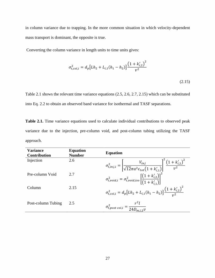
27

in column variance due to trapping. In the more common situation in which velocity-dependent

mass transport is dominant, the opposite is true.

Converting the column variance in length units to time units gives:

𝜎𝑡,𝑐𝑜𝑙,𝑖2 = 𝑑𝑝[𝐿ℎ2 + 𝐿𝑖,1(ℎ1 − ℎ2)]

(1 + 𝑘𝑖,2′ )

2

𝑣2

(2.15)

Table 2.1 shows the relevant time variance equations (2.5, 2.6, 2.7, 2.15) which can be substituted

into Eq. 2.2 to obtain an observed band variance for isothermal and TASF separations.

Table 2.1. Time variance equations used to calculate individual contributions to observed peak

variance due to the injection, pre-column void, and post-column tubing utilizing the TASF

approach.

Variance

Contribution

Equation

Number Equation

Injection 2.6

𝜎𝑡,𝑖𝑛𝑗,𝑖2 = [

𝑉𝑖𝑛𝑗

√12𝜋𝑎2𝜖𝑡𝑜𝑡(1 + 𝑘𝑖,1′ )

]

2(1 + 𝑘𝑖,2

′ )2

𝑣2

Pre-column Void 2.7 𝜎𝑡,𝑣𝑜𝑖𝑑,𝑖

2 = 𝜎𝑡,𝑣𝑜𝑖𝑑,𝑖𝑠𝑜2 [

(1 + 𝑘𝑖,2′ )

(1 + 𝑘𝑖,1′ )

]

2

Column 2.15 𝜎𝑡,𝑐𝑜𝑙,𝑖

2 = 𝑑𝑝[𝐿ℎ2 + 𝐿𝑖,1(ℎ1 − ℎ2)](1 + 𝑘𝑖,2

′ )2

𝑣2

Post-column Tubing 2.5 𝜎𝑡,𝑝𝑜𝑠𝑡 𝑐𝑜𝑙,𝑖

2 =𝑟2𝑙

24𝐷𝑚,𝑖,2𝑣

28

2.3 MATERIALS AND METHODS

2.3.1 Reagents and solutions

Methyl, ethyl, n-propyl, and n-butyl esters of p-hydroxybenzoate (parabens) were purchased from

Sigma-Aldrich (St. Louis, MO). Standard solutions of each paraben were prepared by first

dissolving in acetonitrile, then diluting to the desired concentration and solvent composition with

deionized water. DI water was from an in-house Millipore Milli-Q Synthesis A10 water

purification system (Billerica, MA) and was used without further treatment. Phosphoric acid was

from Fisher Scientific (HPLC grade, Fair Lawn, NJ), and HPLC grade acetonitrile was from

Spectrum Chemical (New Brunswick, NJ). All mobile phases were vacuum degassed and filtered

twice through 0.45 μm nylon filters (Millipore).

2.3.2 van`t Hoff retention studies

2.3.2.1 Instrumentation

A Jasco X-LC 3000 system consisting of a 3059AS autosampler, dual 3085PU semi-micro pumps,

3080DG degasser, 3080MX high pressure mixer, CO-2060 thermostated column compartment,

3177UV variable wavelength UV absorbance detector, and LC-Net II/ADC from Jasco Inc.

(Easton, MD) was used to evaluate the temperature dependence of solute retention. Data analysis

and instrument module control was achieved with EZChrom Elite software from Agilent

Technologies (version 3.2.1, Santa Clara, CA).

2.3.2.2 Chromatographic conditions

A mixture of 25 μM uracil and 50 μM methylparaben, ethylparaben, propylparaben and

butylparaben was made in mobile phase. Samples were injected onto a Waters Acquity BEH C18

column (50 mm x 1.0 mm I.D.; 1.7 μm dp; Waters Corp., Millford, MA). Isocratic separations were

29

made at a flow rate of 200 μL/min with a mobile phase consisting of 80% 10 mM H3PO4, pH 2.7,

20% acetonitrile. The column temperature was varied from 25 to 75 °C in 10 °C steps, the injection

volume was 1.0 μL, and peaks were detected by absorbance of UV light at 210 and 220 nm.

Injections at each temperature were performed in triplicate with the order of the subsequent

temperature analysis selected at random.

2.3.3 TASF instrumentation and chromatographic conditions

2.3.3.1 Column preparation

Figure 2.1 shows a schematic of the instrument used for TASF separations. Capillary columns

were prepared by packing 1.7 μm BEH C18 particles (Waters) into 150 μm I.D. fused-silica

capillaries from Polymicro Technologies (Phoenix, AZ). Columns were fritted by sintering 2 μm,

solid borosilicate spheres (Thermo Scientific, Fremont, CA) into the end of the column blank using

an electrical arc. Particles were slurried in isopropanol (Spectrum) at a concentration of 50 mg/mL,

sonicated for 25 minutes and packed using the downward slurry method at 27500 psi using a Model

DSHF-302 pneumatic amplification pump from Haskel (Burbank, CA). The packing solvent was

acetone (Sigma). Care was taken to pack columns of defined length, ca. 5-6 cm, by limiting the

volume of slurry, and subsequent mass of particles, loaded into the packing system. This allowed

columns to be packed leaving a 2 cm section free of stationary phase at the head of the column.

2.3.3.2 TASF instrumentation

Packed columns were fitted directly to a Cheminert injection valve (Model 07Y-03BH, VICI

Valco, Houston, TX) equipped with a 2 μL sample loop. The sample loop was over-filled with

sample. Injection volume was controlled by controlling the injection time. By this means we

achieved estimated injection volumes from 45 to 1950 nL. A PeakSimple module and associated

30

software (Version 393, SRI Instruments, Las Vegas, NV) were used to actuate the valve. An

Ultimate 3000 RSLCnano high pressure gradient pump (Thermo Scientific, Sunnyvale, CA) with

a an upper pressure limit of 800 bar delivered mobile phase and UV absorbance detection at 210

nm was achieved by a Waters Acquity TUV detector equipped with a 10 nL flow cell (Waters).

Data acquisition and export was achieved through connection of the analog output of the Acquity

TUV to the Jasco ADC described in the van`t Hoff studies. The ADC sampling frequency was 25

Hz, with analysis performed using PeakFit (v4.12, Systat Software, Inc., San Jose, CA).

As shown in Figure 1.1 two different temperature control assemblies were used to regulate column

temperature during the chromatographic run. A Peltier based thermoelectric cooling element

(TEC) from Custom Thermoelectic (part number 03111-5L31-03CF, Bishopville, MD) controlled

the first 7 mm of the column. Utilization of a TEC allowed first cooling the head of the column to

5 °C for 30 s during the injection process, followed by a rapid heating period to the separation

temperature of 60 °C by reversing TEC polarity. To promote rapid heat transfer between the TEC

and column a gallium-indium based eutectic was used at the interface between the TEC and

column [85, 86]. After the desired focusing time TEC polarity was changed manually using a two

position switch. An Agilent 6286A DC power supply powered the TEC, temperature was regulated

by manually tuning the current delivered at fixed potential. A Type T thermocouple (COCO-003,

Omega, Stamford, CT) and a Eurotherm 2416 temperature controller (Invensys Eurotherm,

Ashburn, VA) were used to monitor TEC temperature. Over the course of a day’s experiments

temperature was found to be relatively stable, ±1 °C. The TEC was fixed to a custom aluminum,

water cooled heat sink. A chilled ethylene glycol/water mixture was used to regulate heat sink

temperature. The flow rate for the ethylene glycol/water mixture was 1 L/min; it was delivered by

a Kryo-Thermostat WK 5 chilled circulator (Lauda-Brinkmann, Delran, NJ).

31

The second, isothermal section of the column was heated using a Love Model 1500 proportional-

integral-derivative (PID) controller (Dwyer Instruments, Michigan City, IN) connected to a

Kapton resistive heater (KHLV-103/10-P, Omega). The heater was attached to an aluminum block

onto which the column was placed. A temperature sensor (SA1-RTD, Omega) was fitted inside

the aluminum block and the signal was fed back to the controller; temperature control precision in

the isothermal section of the column was found to be about ±0.1 °C.

2.3.3.3 Injection volume studies

A series of 15 injection volumes from 45 to 1050 nL were performed with and without transiently

cooling the head of the column to test the ability of the TASF methodology to alleviate dispersion

due to pre-column volumes and volume overload. The column used in all injection volume

experiments was 60 mm x 150 μm I.D. and left with a 2 cm void. The flow rate was 3 μL/min, the

mobile phase was 80:20 10 mM H3PO4/acetonitrile and the UV detection wavelength was 210 nm.

Isothermal separations utilized a column temperature of 60 °C. TASF separations employed the

same analysis temperature; the focusing temperature was set to 5 °C. The head of the column was

held at this temperature for 30 s before manually reversing the polarity on the TEC, heating the

column to 60 °C. Isothermal column backpressure was near 330 bar and 470 bar at the 5 °C

focusing temperature. Samples were made in mobile phase at concentrations such that the mass of

each solute injected onto the column was between 3.5 and 9 ng. Table A2.3 provides details

regarding injection volume and sample concentrations used.

2.3.3.4 Limit of quantitation study

Separations were performed with two injection volumes, 60 and 1875 nL. After determining the

ethylparaben limit of quantitation for the Acquity TUV detector using the 10σ value for detector

noise, solute concentrations for each injection volume were selected. The 60 nL injections were

32

performed with samples composed of 1.25 μM ethylparaben; the 1875 nL sample was made at 100

nM. The chromatographic conditions for these separations were nominally identical to those used

in the injection volume studies described in Section 2.4.3.3 with one notable difference. Focusing

conditions were tailored for the separation of ethylparaben to increase usable injection volumes

for TASF separations. Ethylparaben optimization was performed by increasing the focusing time

from 30 to 45 s for the 1875 nL sample. A detailed description related to selection of this focusing

time is reserved for Section 2.4.4.

The following procedure was used to address issues related to carryover between subsequent

injections. Two new 2.0 mL glass syringes from Hamilton (Hamilton Company, Reno, NV) were

used, the first to flush the injection valve with acetonitrile between samples; the second for the

paraben samples. The paraben sample syringe was rinsed three times with acetonitrile before

changing to a different concentration sample. Before injection of paraben samples onto the column,

0.5 mL of acetonitrile was flushed through the 2 μL sample loop while the valve was in the load-

position. The valve was actuated to the inject-position and mobile phase was passed through the

sample loop for five minutes at a flow rate of 3 μL/min. An injection blank consisting of mobile

phase was performed to confirm no sample carryover following this cleaning procedure. This

procedure was repeated between samples.

2.4 RESULTS AND DISCUSSION

2.4.1 Temperature dependence of retention factors

A series of van`t Hoff studies were performed using a commercially available Acquity BEH C18

column prior to implementation of TASF experiments. Partial molar enthalpies of retention for

each solute were determined from van`t Hoff plots (Eq. A1) and retention data over the 25-75 °C

33

temperature range (Table 2.2). Inspection of residuals indicated there was no significant change in

retention enthalpy with temperature. The high degree of linearity allowed extrapolation to the sub-

ambient focusing temperature of 5 °C. The ability to predict solute retention factors at specific

focusing and separation temperatures was critical to modeling the potential of the TASF approach.

Table 2.2. Partial molar enthalpies of retention for methylparaben through butylparaben obtained

from slopes of the van`t Hoff plots (Figure A1.1). Chromatographic conditions can be found in

section 2.4.2.2.

Solute ∆H0/R (K) Error Intercept Error

Methylparaben 1999 11 -5.09 0.03

Ethylparaben 2219 15 -4.87 0.05

Propylparaben 2566 21 -4.98 0.07

Butylparaben 2961 26 -5.24 0.08

2.4.2 Simulation of TASF chromatograms

Equations 2.5, 2.6, 2.7 and 2.15 were used to determine the void, column, and post-column

variances and assess the relative contribution of experimentally accessible parameters on observed

peak variance. To determine the total dispersion of a hypothetical Gaussian peak with no volume

overload, 𝜎𝑡,𝐺2 combination Eqs. 2.5, 2.7, and 2.15 yield:

𝜎𝑡,𝐺,𝑖2 = 𝜎𝑡,𝑣𝑜𝑖𝑑,𝑖

2 + 𝜎𝑡,𝑐𝑜𝑙,𝑖2 + 𝜎𝑡,𝑝𝑜𝑠𝑡 𝑐𝑜𝑙,𝑖

2

(2.16)

Assuming a rectangular injection plug the variance due to injection was redefined as:

𝜎𝑡,𝐵,𝑖2 = 𝜎𝑡,𝑖𝑛𝑗,𝑖

2

(2.17)

34

where 𝜎𝑡,𝐵,𝑖2 describes the variance of a rectangle.

Solving the convolution integral [19] for a rectangular pulse and a Gaussian distribution yields:

𝐶(𝑡) =𝐶0

2√12𝜎𝑡,𝐵,𝑖

[erf√12𝜎𝑡,𝐵,𝑖 − (𝑡 − 𝑡𝑅,𝑖)

√2𝜎𝑡,𝐺,𝑖

+ erf(𝑡 − 𝑡𝑅,𝑖)

√2𝜎𝑡,𝐺,𝑖

]

(2.18)

upon substitution of Eqs. 2.16 and 2.17 where 𝐶0 is sample concentration and 𝑡𝑅,𝑖 is the retention

time for solute 𝑖. The equation used to determine 𝑡𝑅,𝑖 is provided in section A1.2.2. A total of ten

injection volumes were simulated by substitution of the values reported in Table 2.3 into each term

of Eqs. 2.16 and 2.17. Injection volumes used in calculations are reported in Table A1.2.

35

Table 2.3. Parameters involved in isothermal and TASF simulations.

Parameter Determination Value

ts 0.5 min

Vinj 45-1050 nL (See Table A2.2)

F 3 μL/min

Tf 5 °C

Tsep 60 °C

van`t Hoff Plot Slope Experiment See Table 2.2

van`t Hoff Plot Intercept

Dm (310 K) Literature [70, 87] See Table A1.1

η(T) Literature [26, 88] See Eq. A1.2

ϵtot Literature [89] 0.537

A

Literature [84]

20

B 4.5

C 0.01

D 0.42

n 1

dp 1.7 μm

L 6.0 cm

φ 0.2

𝜎𝑡,𝑣𝑜𝑖𝑑,𝑖𝑠𝑜2 Experiment 0.000571 min2

dpost col 25 μm

lpost col 25 cm

36

Figure 2.2 shows two overlays generated from Eq. 2.18. The blue trace in both panels illustrates

the effect of a 5 °C focusing temperature on the observed chromatogram for two injection volumes,

45 and 1050 nL. These injection volumes were selected to mimic experimental results. Using our

system the smallest achievable injection volume was 45 nL. The largest sample used in the

injection volume studies was 1050 nL. In order of elution, peaks were simulated for uracil,

methylparaben, ethylparaben, propylparaben, and butylparaben using appropriate van`t Hoff

parameters and diffusion coefficients. In this calculation uracil was used to mark system dead time

and was defined to have no retention at either the focusing or separation temperatures. Due to this

definition uracil peak shape does not improve when the TASF approach is used at either injection

volume. TASF mitigates pre-column induced dispersion. Simulations assumed all pre-column

dispersion was due to volume overload and the pre-column void. For the 45 nL injection volume

shown in panel A peak heights increased from 15.9 and 15.1 to 34.9 and 30.4 units for

methylparaben and ethylparaben when using TASF. To determine the influence of the pre-column

void on observed peak width a hypothetical system with no pre-column void, i.e. 𝜎𝑡,𝑣𝑜𝑖𝑑,𝑖2 = 0, was

simulated. Figure A1.2 demonstrates the influence of the pre-column void with 5 and 45 nL

injections. A 5 nL injection volume was also selected because it corresponds to just under 1% of

the column volume, analogous to a commonly used 1 μL injection onto a 5 cm x 2.1 mm I.D.

column. Under the simulated conditions with a 5 nL injection volume, implementation of TASF

actually degrades column efficiency by 22% (methylparaben) due to the reduction in column

efficiency at 5 °C. Increasing the injection volume to 45 nL, still without a pre-column void,

already shows improvement in observed column efficiency when using TASF. This result indicates

that a 45 nL injection volume does correspond to volume overload for this column.

37

Figure 2.2. Simulated isothermal (───) and TASF (───) separations of paraben mixtures made

in mobile phase generated using Eq. 2.17. The first peak in each panel is uracil, the void time

marker was defined to have no retention at separation and focusing temperatures. A 45 nL injection

is shown in panel A, panel B shows a 1050 nL injection. Peak area for each solute was held constant

at both injection volumes to allow easy comparison of peak shape between injection volumes.

Values used for simulations can be found in Table 2.3.

38

Panel B of Figure 2.2 demonstrates the ability of TASF to focus large volume samples onto the

head of the column. Defining the liquid volume of the column as the fluid volume of the column

(𝜋𝑎2𝐿𝜖𝑡𝑜𝑡) excluding the pre-column void, a 1050 nL injection corresponds to 160% of the column

volume. The simulated chromatogram clearly shows significant volume overload. Although TASF

with a 5 °C focusing temperature decreased peak width for all solutes, this temperature (5 °C) did

not suffice to increase retention for methylparaben and ethylparaben to create Gaussian peaks.

Retention factors calculated from the van`t Hoff parameters in Table 2.2 are shown in Table A1.1.

To solve this problem further reductions focusing temperature would be required for further

reductions in peak width for low retention solutes such as methylparaben and ethylparaben.

In order to visualize the effect of TASF over a wide range of injection volumes a metric easily

relatable to experimental data was required. The flat-topped peaks obtained at large injection

volumes are not well fit by various Gaussian modifications, e.g. exponentially modified Gaussian

(EMG) or 5-parameter EMG. However, experimental values for the full width at half maximum

(FWHM) can be measured readily. The following approximation was made to allow generation of

FWHM vs. Vinj plots.

𝐹𝑊𝐻𝑀 = [12𝜎𝑡,𝐵2 + (2√2 ln 2 𝜎𝑡,𝐺)

2]

12⁄

(2.19)

Equation 2.19 combines the FWHM of a Gaussian peak, 𝜎𝑡,𝐺, calculated from Eq. 2.16 and adds

it to the injection variance width, 𝜎𝑡,𝐵2 . The square root of the sum accurately estimates the FWHM

of peaks from purely Gaussian to purely rectangular over the range of values used here with a

maximum error of 12%. Systematic increases in the overestimation values for FWHM values with

increased injection value were observed. Figure 2.3 was generated from a series of ten injection

39

volumes ranging from 45 to 1050 nL and values in Table 2.2. Panels A-D correspond to

methylparaben through butylparaben; TASF separations with a 5 °C focusing temperature are

shown in blue. Isothermal separations at 60 °C are in black. Red dashed lines indicate a 5%

increase in FWHM for 45 nL isothermal injections. A 5% increase in FWHM is approximately

equal to a 10% reduction in column efficiency. Benefits obtainable with TASF across all injection

volumes are most prominent for low retention solutes at low injection volumes and high retention

solutes at large injection volumes. At 5 °C TASF reduces the observed FWHM for a 45 nL

injection of methylparaben by a factor of 2.2, speaking to the method’s ability to reduce pre-

column dispersion. TASF is only able to reduce the width of the observed small injection volume

butylparaben band by 5% for a 45 nL injection. This explains why the relative difference between

FWHM values for the isothermal and TASF separations show in panels A-D of Figure 2.3

decreases with increasing isothermal retention factor. At injection volumes greater than the column

volume TASF is able to limit the rate of increase for observed FWHM values. This effect is most

apparent when comparing panels A and D for methylparaben and butylparaben. At an injection

volume of 450 nL the TASF FWHM value for methylparaben has risen above the 5% increase line

for a 45 nL injection. This does not occur for butylparaben at 5 °C until about 1500 nL.

40

Figure 2.3. Simulated isothermal (●) and TASF (●) separations where the injection volume of

paraben samples made in solvent systems identical to the mobile phase was varied from 45 to 1050

nL. Panels A, B, C, and D correspond to simulations for methylparaben through butylparaben,

respectively. Red dashed lines represent a 5% increase in the FWHM for a 45 nL isothermal

injection for each solute. Increases in simulated FWHM values with increasing in injection volume

were due to the pre-column void and volume overload. TASF reduced peak FWHM for all solutes

across all injection volumes under the conditions reported in Table 2.3.

41

2.4.3 Experimental determination of the effect of TASF on peak width

A series of fifteen injection volumes were performed under isothermal and TASF conditions with

paraben samples prepared in mobile phase. Example chromatograms are shown in Figure 2.4; both

panels display TASF separations with 5 °C focusing temperatures in blue and 60 °C isothermal

separations in black. These experimental results mirror the simulated results of Figure 2.2. Panel

A corresponds to a 45 nL injection and B a 1050 nL injection. Estimating the column volume to

be 640 nL, the 45 nL injection corresponded to 7% of the column volume and the 1050 nL injection

160%. The increase in peak height for TASF analyses was the method’s most obvious advantage.

The peak height values for methylparaben and ethylparaben in panel A of Figure 2.4 increased by

20% relative to their peaks in the isothermal separation. At both injection volumes, Figure 2.4

panels A and B, methylparaben, ethylparaben, and propylparaben benefitted most from TASF. At

the retention factor extremes characterized by uracil, no retention, and butylparaben, k’60 °C = 38.4,

the influence of TASF was reduced. Uracil, with k’ = 0, cannot be focused and butylparaben with

its large k’ is focused without the assistance of reduced temperature. Of course, TASF would

improve the butylparaben peak width had larger volumes been injected. These results indicate that

under experimental conditions there was an optimal retention factor ratio present between the

focusing and separation segments of the column. Panel B of Figure 2.4 demonstrates the potential

for TASF to minimize volume overload. The inset in panel B shows the propylparaben peak from

an isothermal separation with a 1050 nL injection volume. It shows that flat topped peaks

characteristic of volume overload were obtained even for relatively high retention compounds.

When TASF was used the large volume sample was effectively focused in the cold trap increasing

peak heights for methylparaben, ethylparaben, and propylparaben by factors of 3.2, 4.2 and 3.4,

respectively.

42

Figure 2.4. Demonstration of the potentiation for the TASF approach to reduce observed peak

width for samples made in mobile phase at multiple injection volumes. Isothermal (───)

separations were performed at 60 °C. A 5 °C focusing temperature and 30 s focusing time were

used with the TASF approach (───). Panel A shows results from a 45 nL injection, panel B a

1050 nL injection. The pop-out in panel B illustrates the flat topped peak profiles observed for the

isothermal propylparaben peak.

43

Figure 2.5 shows measured peak width at half height for each solute as a function of injection

volume. These experimental results correspond to the simulated results in Figure 2.3. Panels A, B,

C, and D of Figure 2.5 present the results of these experiments for methylparaben, ethylparaben,

propylparaben, and butylparaben, respectively. Isothermal separations are plotted as black circles;

TASF experiments are blue. Red dashed lines correspond to a 5% increase in FWHM for a 45 nL

injection. Error bars were calculated from the standard error for each measured FWHM, with n =

3. Qualitatively, the shape of the plots and relative increase in FWHM between isothermal and

TASF experiments mimic the results predicted by the simulations. Low retention solutes are more

susceptible to volume overload-related increases in FWHM. The ability of TASF to limit the rate

of FWHM increase with increasing injection volume for samples made in mobile phase was

impressive. Methylparaben, with an isothermal retention factor of 2.5 was the only solute tested

where volume overload induced dispersion increased FWHM values by more than 5% of the value

for a 45 nL injection with TASF on. These results demonstrate experimentally the capability of

TASF to focus all samples made in mobile phase despite a large pre-column void and modest

focusing temperature of 5 °C.

While the guidance from the theory is quite good, there are discrepancies between the predicted

and experimental results. For example, the predicted benefit of TASF for small volume injections

and low k’ solutes is better than we realize experimentally. One factor is our uncertainty about the

variance contributed by the void. This variance is most important for low k’ compounds. Another

factor is our lack of knowledge of the actual temperature inside the column. We model the changes

in temperature as a step function, but they are actually not. In addition, the temperature changes

are initiated by a manual switch. We are in the process of addressing these limitations.

44

Figure 2.5. Results from volume overload experiments performed under isothermal (●) and TASF

(●) conditions with paraben mixtures made in mobile phase. Panels A, B, C, and D correspond to

methylparaben through butylparaben peaks, respectively. Red dashed lines represent a 5% increase

in the FWHM for a 45 nL injection for each solute. TASF was able to reduce observed FWHM

values relative to its isothermal counterpart for every solute at each injection volume.

45

2.4.4 Improvements in concentration detection limit offered by temperature-assisted solute

focusing

As part of our initial assessment of the practical implementation of the TASF approach, we

evaluated improvements in the concentration detection limits for the targeted determination of

ethylparaben. Assuming constant peak area, reductions in observed peak width due to TASF result

in taller peaks with enhanced S/N ratios. To demonstrate our ability to model the effect of TASF

and realize the benefits in practice, an experiment was designed to address the following question.

Knowing the signal required to be 10-times the standard deviation of the baseline, can you

quantitate an injection using TASF to create a narrow peak at the detection limit from a volume

overloaded injection at a concentration well below the isothermal detection limit?

In this example the standard state retention enthalpy for the target analyte, ethylparaben, was

experimentally determined. Its retention factor and elution velocity in the 5 °C, 7 mm long trapping

section at a flow rate of 3 μL/min were calculated to be 18.0 and 0.15 mm/s. For effective focusing,

the leading edge of the ethylparaben band must remain within the trapping zone, i.e. not elute from

the trap during the focusing time. This condition places a limit on the maximum allowable injection

volume given the defined trap length and temperature. Assuming no dispersion from either the

leading or trailing edges of the ethylparaben band it will take 7 s for the leading edge of the band

to reach the trapping zone and a further 47 s for it to reach the end of the trapping zone. The total

injection time is thus 54 s. The presence of dispersion and other nonidealities of our model will

cause the band’s front edge to reach the end of the trapping zone in a time shorter than 54 s.

Experimentally, a focusing time of 45 s was used with an injection time of 37.5 s (1875 nL).

The chromatograms in Figure 2.6 show the results for two injections of ethylparaben under

isothermal (black traces) and the optimized ethylparaben TASF conditions (blue traces). Panel A

46

shows a 60 nL injection of 1.25 μM ethylparaben in mobile phase with a 30 s focusing time. Due

to the 1.2 s long injection required to achieve a 60 nL injection volume, increasing the focusing

time to 45 s to accommodate larger injection volumes was unnecessary. The red dashed line is at

an absorbance value equal to ten times the standard deviation of the baseline noise. The 60 nL

injection was designed to act as a control and establish the detection limits for the TASF

separations. The detection limit for ethylparaben using the TASF approach and a 60 nL injection

was 7.5×10-14 moles. Panel B shows a more powerful demonstration of TASF’s ability to improve

concentration detection limits. To highlight this, the time axes of panels A and B were plotted to

roughly center the ethylparaben peaks for isothermal and TASF separations, while the length of

each window was held constant at 0.8 minutes. Increasing focusing time and injection volume

resulted in an increase in ethylparaben retention time and peak width. Ethylparaben concentration

in the 1875 nL sample was 100 nM, 1.9×10-13 moles on-column. The most impressive aspect of

the TASF methodology came from the comparison of the 1875 nL isothermal and TASF

separations. A red arrow is used to highlight what we believe to be the severely broadened

ethylparaben peak which is not distinguishable from the baseline noise. The isothermal column is

clearly volume overloaded. Only using TASF we were able to focus the large volume sample,

nearly three times the fluid volume of the column, to achieve a quantifiable peak. This ability

reduced the concentration detection limits for this analysis by a factor of 12.5, relative to the 60

nL injection.

47

Figure 2.6. Chromatograms from the limit of quantitation study performed following optimization

of TASF conditions for the separation of ethylparaben. Ethylparaben concentrations for 60 nL (A)

and 1875 nL (B) injections were 1.25 μM and 100 nM. These concentrations were selected to be

just above the detector’s limit of quantitation, shown by red dashed lines. The TASF approach

offered reductions in peak width and increases in peak height making previously unquantifiable

isothermal analyses (───) quantifiable when implementing TASF (───). The red arrow in panel

B shows what we believe to be the isothermal ethylparaben peak.

48

2.5 CONCLUSIONS

We have investigated the efficacy of temperature assisted on-column solute focusing to ameliorate

all sources of pre-column dispersion and their associated reductions in column efficiency. The

primary advantages to TASF for inducing efficient on-column focusing are as follows.

1. The approach effectively mitigates increases in peak width introduced by injecting

large volumes of samples dissolved in solvents matching the mobile phase. TASF is

orthogonal to solvent-based focusing methods allowing its use to replace or augment

solvent-based methods.

2. A variance based model facilitates accurate in silico simulation of TASF separations

based on solute retention enthalpies, focusing temperature, focusing time, and column

parameters.

3. Optimized TASF analyses will decrease the concentration detection limit when large

volumes with respect to the void volume are injected.

Potential applications of TASF: 1. continuous, online microdicodialysis sampling of for the rapid

quantitation of neurotransmitters [90-92] where large aqueous samples are injected onto a capillary

column operated with less than 5% acetonitrile in the mobile phase and 2. re-focusing fractions of

first dimension effluent sampled and injected onto the second dimension column in capillary online

comprehensive two-dimensional liquid chromatography, LCxLC [93].

49

3.0 TEMPERATURE-BASED ON-COLUMN SOLUTE FOCUSNG IN

CAPILLARY LIQUID CHROMATOGRAPHY REDUCES PEAK BROADENING

FROM PRECOLUMN DISPERSION AND VOLUME OVERLOAD WHEN USED

ALONE OR WITH SOLVENT-BASED FOCUSING

The contents of this chapter were previously published in: Groskreutz, S. R., Horner, A. R. and

Weber, S. G. Journal of Chromatography A, 2015, 1405, 133-139.


3.1 INTRODUCTION

When sample volumes are small and quantitative analysis of low-concentration analytes is the

goal, it is generally advantageous to use capillary liquid chromatography [35]. The advantage

arises from the fact that the use of capillary columns minimizes the dilution of the analytes [18,

94]. With a concentration-sensitive detector, concentration detection limits improve as the injected

volume of the sample increases or the column diameter decreases up to a point, however volume

overload results when the injection volume contribution to observed bandspreading becomes

significant [44, 95]. This contribution of the injected volume to bandspreading is dependent on the

solute retention factor in the sample solvent. If retention is low, injection-related band spreading

can be significant. Volume overload effects are lower for highly retained solutes. Thus, injecting

aqueous samples onto a reversed phase column can be effective at eliminating volume overload as

solutes are retained well while the sample solvent is temporarily acting as the mobile phase. This

concentration effect is termed solvent-based on-column focusing and is a simple solution to the

volume overload problem [48, 94].

50

Temperature also affects retention. Typically in reversed-phase liquid chromatography retention

increases as temperature decreases [68, 96]. Thus, as we have recently shown [97], temperature-

based on-column solute focusing (TASF) can be used to minimize the volume overload problem.

TASF works by maintaining a temperature of a short segment (e.g., 1 cm) at the head of the column

well below the rest of the column temperature for the time period during the injection. Following

sample loading and analyte focusing due to increased retention, the temperature of the column

(focusing) segment is rapidly heated to match the rest of the column. TASF should be most

effective with capillary-scale columns because of their low thermal mass and small radius. The

former permits rapid temperature changes while the latter is responsible for rapid relaxation of

thermal gradients in the column.

Previously, the Greibrokk group exploited sub-ambient column temperatures to focus large-

volume samples of retinyl esters, polyolefin based Irganox antioxidants and ceramides onto the

head of capillary columns [76-80]. High solute hydrophobicity and poor solubility in water

necessitated the use of neat acetonitrile mobile phases. Temperature was left as the only variable

to enhance focusing and control elution. They initiated temperature programs (for the entire

column) at sub-ambient temperatures, ca. 5 °C, to focus these solutes in samples made in 80-100%

acetonitrile. Later Holm et al. developed a column oven with separate hot and cold zones where a

capillary column was moved in-space from the cold zone to a hot zone following temperature-

assisted online preconcentration of Irganox samples dissolved in acetonitrile [81]. Eghabali et al.

also used temperature to enhance detection sensitivity in capillary LC [83]. In this approach a 1

cm long segment of column near the outlet was cooled cryogenically to -20 °C to trap and re-focus

specific proteins within defined regions of the chromatogram. Following focusing, boiling water

51

was used to heat the nitrogen gas flowing around the cooled segment to rapidly release focused

bands in targeted regions of the chromatogram.

In our previous work [97], we demonstrated that TASF decreases volume overload significantly

when the sample is prepared in a liquid with the same composition (chromatographic strength) as

the mobile phase. Here, we demonstrate that TASF is also effective in isocratic elution: 1) when

the sample solvent is weaker than the mobile phase, and 2) when the sample solvent is stronger

than the mobile phase. In the former case, TASF and solvent together dictate the k’ of the solutes

during the injection. In the latter case, TASF makes it possible to inject large volumes. Among

other technical improvements to the TASF system, we have also automated its control and we

demonstrate here its reproducibility in controlling column temperature and focusing for large

volume samples.

3.2 MATERIALS AND METHODS

3.2.1 Reagents and solutions

Methyl, ethyl, and n-propyl esters of p-hydroxybenzoate (parabens) were purchased from Sigma-

Aldrich (St. Louis, MO). Standard solutions of each paraben were prepared by first dissolving in

acetonitrile (AN), then diluting to the desired concentration and solvent composition with

deionized water (DI). Galanin (1-29) (rat) was obtained from Tocris Bioscience (Ellisville, MO).

DI water was from an in-house Milli-Q Synthesis A10 purification system (Billerica, MA) and

used without further treatment. Phosphoric acid (HPLC grade) and LC/MS grade acetonitrile were

from Fisher Scientific (New Brunswick, NJ). Trifluoracetic acid (HPLC grade) and uracil were

also from Sigma-Aldrich.

52

3.2.2 van`t Hoff retention studies using commercial columns

3.2.2.1 Chromatographic instrumentation

A Jasco X-LC system composed of a 3059AS autosampler, dual 3085PU pumps, 3080DG

degasser, 3080MX high pressure mixer, CO-2060 thermostated column compartment, 3177UV

variable wavelength UV absorbance detector and LC-Net II/ADC from Jasco Inc. (Easton, MD)

was used to evaluate the temperature dependence of solute retention. Instrument control and data

analysis was achieved using EzChrom Elite software (version 3.2.1, Agilent Technologies, Santa

Clara, CA)

3.2.2.2 Chromatographic conditions

A total of three van`t Hoff retention studies using a commercially available 1 mm I.D. Waters

Acquity BEH C18 column (50 mm x 1.0 mm I.D.; 1.7 μm dp; Waters Corp., Millford, MA). were

performed for methylparaben, ethylparaben, and propylparaben Solute retention enthalpy values

were determined for mobile phases consisting of 70:30, 80:20 and 90:10 (10 mM H3PO4, pH 2.7:

AN). Column temperature was varied from 25 to 65 °C in 20 °C steps. Samples of 15 μM uracil

and 25 μM of each paraben were made at each mobile phase composition. The injection volume

was 1.0 μL, flow rate was 0.1 mL/min, and peaks were detected by absorbance of UV light at 220

and 254 nm. Injections were performed at each temperature in triplicate. Extra column time was

determined by replacing the column with a zero dead volume union.

3.2.3 Second generation TASF instrumentation and chromatographic conditions

3.2.3.1 Column preparation

Capillary columns used in all TASF experiments were prepared by packing either Acquity BEH

C18 or Acquity CSH C18, 1.7 μm particles (Waters) into 100 or 150 μm I.D. fused-silica

53

capillaries from Polymicro Technologies (Phoenix, AZ). Columns were fritted using an electrical

arc to sinter 2 μm solid borosilicate spheres (Thermo Scientific, Fremont, CA) into the end of the

column blank. Particles were slurried, 65 mg/mL, in isopropanol and sonicated for 20 minutes

prior to packing using the downward slurry method. Fritted blanks were placed into an ultrahigh

pressure column packing fitting adapted from that previously described [98]. A model DSF-150

pneumatic amplification pump from Haskel (Burbank, CA) was used to pack columns at 20,000

psi for 20 minutes. Acetone was used as the packing solvent. Defined length columns, ca. 4.5-6.5

cm, were packed by controlling the mass of particles loaded into the packing reservoir. The

remainder of the capillary blank was packed with 8 μm solid silica spheres (Thermo) for an

additional 20 minutes at 20,000 psi. The silica spheres were slurried at a concentration of 100

mg/mL in a mixture of 50:50 (v/v) isopropanol/water.

3.2.3.2 TASF instrumentation

A 3D rendering of the TASF instrumentation is shown in Figure 3.1. A Thermo Scientific Ultimate

3000 RSLCnano high pressure gradient pump (NCS-3500RS, Germering, Germany) was used to

deliver mobile phase. System pressure was monitored using an externally mounted pressure

transducer (DF2-SS-01-15000, DJ Instruments, Billerica, MA). The outlet of the pressure

transducer was connected to a Cheminert injection valve (C72x-669D, VICI Valco, Houston, TX)

via a 75 μm x 35 cm fused silica nanoViper capillary (Thermo). A second 75 μm x 65 cm

nanoViper capillary, fluidic volume of 2.9 μL, was used as the sample loop. (Note that all injection

volumes were dictated by precisely controlling the period of time the injection loop was in the path

of the column.) The sample loop was loaded by flow from the Ultimate ternary loading pump and

an HP1050 autosampler (Agilent, Waldbronn, Germany). The autosampler injection volume was

set to 75 μL and loading pump flow rate was adjusted to ensure that each sample was introduced

54

Figure 3.1. Schematic of instrument used to implement the TASF approach. TEC and resistive

heaters are shown in gold and red. A loading pump and an autosampler introduced successive

samples into a loop connected to the injection valve. Packed void columns were laid on top of the

focusing segment and connected directly to the valve. The outlet of the column was connected to

the inlet of the detector flow cell using a Teflon sleeve. The insert shows a top- down view of the

injection valve and focusing segment of the column.

55

into the nanoViper injection loop during the previous run. Capillary columns were fitted directly

to the injection valve and the column outlet was connected to an Acquity TUV detector fitted with

a 10 nL flow cell (Waters). Data acquisition at 25 Hz was achieved via connection of the analog

output of the Acquity TUV to the Jasco ADC described in the van`t Hoff studies. Analysis was

performed in MATLAB (MathWorks, Natick, MA) using a simple peak finding algorithm to

automatically find and measure peak full width at half maximum (FWHM). The MATLAB script

used to determine FWHM is provided in Appendix B2.3.

Temperature-based focusing was achieved using a 1.0 x 1.0 cm Peltier thermoelectric cooling

element (TEC) from Custom Thermoelectric (part number 04801-9G30-34RB, Bishopville, MD).

To enhance heat transfer between the TEC and the column a gallium-indium eutectic was used at

the interface between the TEC and column. An Agilent E3646A DC power supply was used to

drive the TEC. TEC temperature was set manually by adjusting the current delivered by the power

supply at fixed potential. A Type T thermocouple (COCO-003, Omega, Stamford, CT) fixed to

the surface of the TEC was connected to a National Instruments 9213 16-channel high speed

thermocouple input module (Austin, TX). TEC polarity was changed using a simple electronically

controlled relay circuit. The TEC was mounted to a custom aluminum, liquid cooled heat sink. A

Kryo-Thermostat WK 5 chilled circulator (Lauda-Brinkmann, Delran, NJ) was used to pump an

ethylene glycol/water mixture at 1 L/min through the heat sink.

The isothermal section of the column was heated resistively in a manner similar that used

previously [92, 99]. Briefly, a Love Model 1500 proportional-integral-derivative (PID) controller

(Dwyer Instruments, Michigan City, IN) was used to control a Kapton resistive heater (KHLV-

103/10-P, Omega). The heater was attached to an aluminum block and an SA1-RTD temperature

sensor (Omega) was used to monitor temperature.

56

Instrument control and acquisition of temperature and pressure profiles was collected at 10 Hz

using a simple LabVIEW program (National Instruments) written in-house. The injection valve

and TEC polarity were also controlled using LabVIEW via an NI 9403 digital I/O module, pressure

and HP1050 autosampler remote start signals were monitored using a NI USB-6008 DAQ.

3.2.3.3 TASF reproducibility study

To evaluate the instrumental improvements and assess the speed of column temperature and

pressure transients, an eighty-five injection sequence was performed. The column was an 8.9 cm-

long, 150 μm I.D capillary packed with 1.7 μm Acquity BEH C18 particles in the downstream 6.5

cm. The 2.4 cm segment of the column at the inlet, which is inside the fitting holding it (see Figure

3.1) to the injection valve and also includes the space between the valve and edge of the TEC, was

packed with 8 μm dp solid silica spheres. We refer to such columns as “packed void” columns. In

all subsequent references to column length only the length of the stationary phase is reported; a

2.4 cm packed void segment is assumed. Flow rate was 4.0 μL/min, the mobile phase was 75:25

10 mM H3PO4/AN and the detection wavelength was 254 nm. A focusing time of 35 s was used;

𝑇1 and 𝑇2 were set to 0 and 65 °C, respectively. Each run was set to 10 minutes (an 11.5-minute

total cycle time including time for 1050AS to perform the injection) with the whole experiment

lasting 975 minutes.

3.2.3.4 Injection volume study

To replicate the results of our previous work with the new TASF system a series of ten timed

injection volumes in the range of 30 to 750 nL were made in triplicate with and without TASF.

The column was an Acquity BEH C18 packed void column, 4.7 cm x 150 μm I.D, 1.7 μm dp. Flow

rate was 4.5 μL/min, the mobile phase was 80:20 10 mM H3PO4/AN and the detection wavelength

57

was 254 nm. Column temperature was 70 °C. TASF separations employed focusing temperatures

of 5 °C, focusing times of 15 s. Samples were made in mobile phase. Table B2.2 provides details

regarding injection volumes and sample concentrations used.

3.2.3.5 Solvent- and temperature-focusing injection volume study

The complementary nature of solvent- and temperature-based on-column focusing was

demonstrated for injection volumes ranging from 100-2000 nL. Isothermal and TASF injections

of uracil, methylparaben, ethylparaben, and propylparaben were made in triplicate with sample

compositions of 80:20 (matching the mobile phase) and 95:5 10 mM H3PO4/AN to evaluate the

effect of solvent- and temperature-based focusing when both focusing techniques were used

together. An Acquity BEH C18 packed void column as described in Section 3.2.3.3 was used. The

fluidic volume of the column, excluding the packed void, was estimated to be 450 nL. The flow

rate was 3 μL/min; the mobile phase and detection wavelengths were the same as Section 3.2.3.4.

Column and focusing temperatures were reduced to -5 and 62.5 °C to enhance temperature-based

focusing. To accommodate the larger injection volumes, the focusing time was increased to 45 s.

Table B2.3 provides details about the injection volumes and sample concentrations used.

3.2.3.6 TASF applied to increasing the sensitivity for the peptide galanin

Isothermal and TASF separations were performed on samples of 100 nM galanin prepared in 80:20

water/AN. Injection volumes of 500 nL were made onto a packed void Acquity CSH C18 column

(6.0 cm x 100 μm I.D., 1.7 μm dp) with the mobile phase composition set to 85:15 0.1%

trifluoroacetic acid/AN. Flow rate and detection wavelength were 0.85 μL/min and 214 nm,

respectively. Isothermal separations were performed at 65 °C. TASF separations utilized focusing

temperatures of -10 °C and focusing times of 40 s.

58


3.3.1 Temperature dependence of retention factors

A commercially available Acquity BEH C18 column was used to determine retention factors under

the various solvent and temperature conditions used in TASF experiments. Retention factors were

corrected for extra-column volume using Eq. B2.1 in Appendix B. Partial molar enthalpies (Table

B2.1) for each solute were determined from the van`t Hoff plots shown in Figure B2.3 (Eq. B2.2),

using retention data collected over the 25-65 °C temperature range. Residual plots showed no

evidence of significant curvature, thus there was no substantial change in retention enthalpy with

temperature. We took advantage of this linearity to extrapolate retention factors to sub-ambient

column temperatures.

3.3.2 TASF instrumentation

We improved the technical capabilities of the TASF system by adding electronic control with data

logging, and incorporating the TASF system into the instrument control process of a commercial

autosampler. In addition, the physical apparatus is now robust and easily incorporated into a

capillary chromatography system. Figure 3.1 is a 3D rendering of the arrangement of the valve,

column, TEC, resistive heater, pressure transducer, and other related components of the TASF

system. The inset panel shows the placement of the TEC and capillary column. The TEC (1.0 cm

x 1.0 cm x 1.6 mm, shown in gold) was mounted to a custom aluminum heat sink fit inside a PVC

fixture machined to hold the TEC-heat sink assembly and resistive heater for the downstream

separation segment of the column. The resistive heater (shown in red) used to heat the separation

segment of the column was maintained at constant temperature (𝑇2) throughout the run. The TEC

changes the column temperature of the focusing segment from 𝑇1 to 𝑇2 and back again. It is clear

59

from the inset panel of Figure 3.1 that the majority of the thermal mass requiring the temperature

change is within the TEC, not the 360 μm O.D. column. Therefore, selection of a thin (low thermal

mass), high power TEC is desirable for rapid temperature changes from 𝑇1 to 𝑇2. The TEC is rated

at 10.9 W, significantly more powerful than the TEC (6.3 W) used in our previous work [97] and

is capable of changing temperatures of the focusing segment by approximately 60-70 oC (𝑇2 - 𝑇1).

The operator can choose actual 𝑇1 and 𝑇2 values according to the need. For example, to concentrate

samples with low retention solutes (at the column temperature and in the sample solvent), a low

𝑇1 would be appropriate to increase focusing and decrease volume overload. However, there is an

attendant limitation on how high 𝑇2 can be when 𝑇1 is low. If the desire is for high column

temperature, then a higher focusing temperature (𝑇1) can be used, but this is accompanied by the

need to inject smaller volumes to avoid volume overload for the lower retention solutes.

To realize the benefits of TASF, solutes must arrive at the cooled trapping segment at the same

time. Thus, in our earlier work we advocated leaving the first ca. 2 cm of capillary – the portion

located within the injection valve and fittings – unpacked. The same concept was applied in the

work of Holm et al. work using temperature-based focusing with Irganox antioxidants [81]. This

void introduced a pre-column volume of more than 350 nL for the 150 um I.D. columns used in

our work. The void added significantly to pre-column dispersion and introduced a time delay on

the order of 5 s to the separation. To address these problems, we created so-called “packed void”

capillary columns. First, the column blank was packed with stationary phase to the desired length.

Then the remainder of the capillary was packed with non-interacting solid silica spheres. The silica

spheres do not contribute to retention; they act only to fill up the empty space in front of the

column. Packing the void reduces the pre-column volume by roughly 65% to 120 nL. Reduced

60

pre-column volume shortened the time delay, but more importantly the particles significantly

reduce pre-column dispersion seen in the absence of temperature- or solvent-based focusing.

To demonstrate the effectiveness of the TASF instrumentation for routine separations and evaluate

the speed of column temperature and pressure transients an overnight injection sequence was

performed consisting of eighty-five injections. Each run was 10 minutes; cycle time was 11.5

minutes when accounting for the autosampler injection time. The whole sequence lasted just over

16 hours. Figure 3.2 shows overlays of focusing temperature and column pressure. The colored

overlays correspond to the first TASF separation performed in the sequence. Black temperature

and pressure traces represent traces from the last injection. There are no visible changes in the

pressure profile and a minimal deviation between the first and last temperature profiles over the

course of the sequence. TEC temperature reached 90% of the set value (58.5 °C) in 5.6 s; this

corresponds to a temperature gradient of 625 °C/min. Column pressure transients mirrored those

for temperature with minimal time lag. This is due to the low thermal mass and high thermal

conductivity of fused silica capillaries [100]. We refer interested readers to Appendix B2.2 for

further discussion regarding TASF instrumentation.

61

Figure 3.2. Focusing segment temperature profiles are shown in red (───) and column pressure

traces in blue (───) for the first TASF separation performed in the 85 injection sequence. Black

traces (───) show temperature and pressure profiles for the last TASF separation in the sequence.

Column temperature was 65 °C, focusing temperature was 0 °C; the focusing time was 35 s.

62

3.3.3 Effect of TASF on peak width

Figure B2.4 (see Appendix B) shows representative chromatograms with and without TASF for

small (30 nL) and large (750 nL) injections of parabens prepared in mobile phase. Figure B2.5

shows measured peak width at half height for each solute as a function of injection volume. Solute

retention factor dictates how susceptible an analyte is to volume overload. Here, we have chosen

solutes and conditions to give a range of 3.0 (methylparaben) < k’ < 17.5 (propylparaben;

ethylparaben has a k’ of 7.1) at 𝑇2 = 70 °C. The data show that for this range of practically useful

isocratic retention factors, TASF alone can be effective. At the 5 °C focusing temperature retention

factors for each solute are greater: 11.7, 32.0 and 99.4, respectively. (Retention factors were

calculated based on the van ‘t Hoff studies detailed in Section 3.2.1. For further details, see section

B2.1 of Appendix B.) Under these conditions, TASF is able to limit the increase in FWHM to 5%

for injection volumes up to nearly 100% of the column volume (450 nL) for methylparaben and

165% for ethylparaben and propylparaben. These data are similar to our published data [97]

confirming, as expected, that technical changes did not alter the essential function of the TASF

device.

3.3.4 Combination of solvent- and temperature-based on-column solute focusing

Figure 3.3 shows results from the large-volume injections performed under isothermal and TASF

conditions with paraben samples prepared in 80:20 and 95:5 10 mM H3PO4/AN. These

experiments were conducted to demonstrate the effectiveness the combination of solvent- and

temperature-based on-column focusing can have to limit increases in peak FWHM for sample

volumes up to 450% of the column volume. Panels A, B, and C present results for methylparaben,

ethylparaben, and propylparaben, respectively. Error bars are the standard error for each measured

FWHM, with n = 3.

63

Figure 3.3. Peak width vs. injection volume for solvent- and temperature-based focusing made

under isothermal and TASF conditions. Panels A, B, and C correspond to methylparaben through

propylparaben peaks, respectively. Black circles represent isothermal separations with sample

made in mobile phase. Red, isothermal with samples in 95:5 phosphate/acetonitrile. TASF

separations with samples made in 95:5 phosphate/acetonitrile are in blue.

64

The benefits of solvent-based on-column focusing are clearly evident from each panel of Figure

3.3. Observed peak width is reduced for every injection volume from 100 nL to 2 μL for each

solute. For the 2 μL injections, representing a volume 450% of the column volume, peak width

values for methylparaben, ethylparaben and propylparaben were reduced from about 40 s

(injection width) when no solvent focusing was present to 5.5, 5.8, and 7.1 s, respectively when

injecting samples made in 95:5 phosphate/AN. TASF and solvent focusing together reduced the

influence of volume overload significantly. FWHM values for the 2 μL injection with solvent- and

temperature-based focusing together were reduced to 1.4, 2.5, and 6.2 s.

Figure 3.4 shows an overlay for 2 μL injections under the three conditions described above. The

black trace shows the result from injecting the paraben mixture made in mobile phase onto an

isothermal column. Clearly, this is unsatisfactory chromatography. The red trace shows the same

sample made in 95:5 phosphate/AN. As expected, chromatographic performance improves when

using solvent-based focusing. Improvement is due to increased solute retention factors in the

sample solvent at the head of the column. Note that injecting a nearly aqueous 2 μL sample onto

the column still does not induce enough on-column focusing to generate a Gaussian peak for

methylparaben. The ethylparaben peak is also significantly broadened. In principle, a completely

aqueous sample would focus more effectively, but not all reversed phase materials perform well

with an aqueous mobile phase. Atypical peak shapes may result for large volume aqueous

injections. The blue trace shows that TASF augments the on-column focusing from solvent. Using

a focusing temperature of -5 °C resulted in peak height increases by factors of 3.4 and 2.2 for

methylparaben and ethylparaben relative to the solvent-focusing-only injection. Better and more

sensitive chromatography can result from using solvent- and temperature-based focusing together.

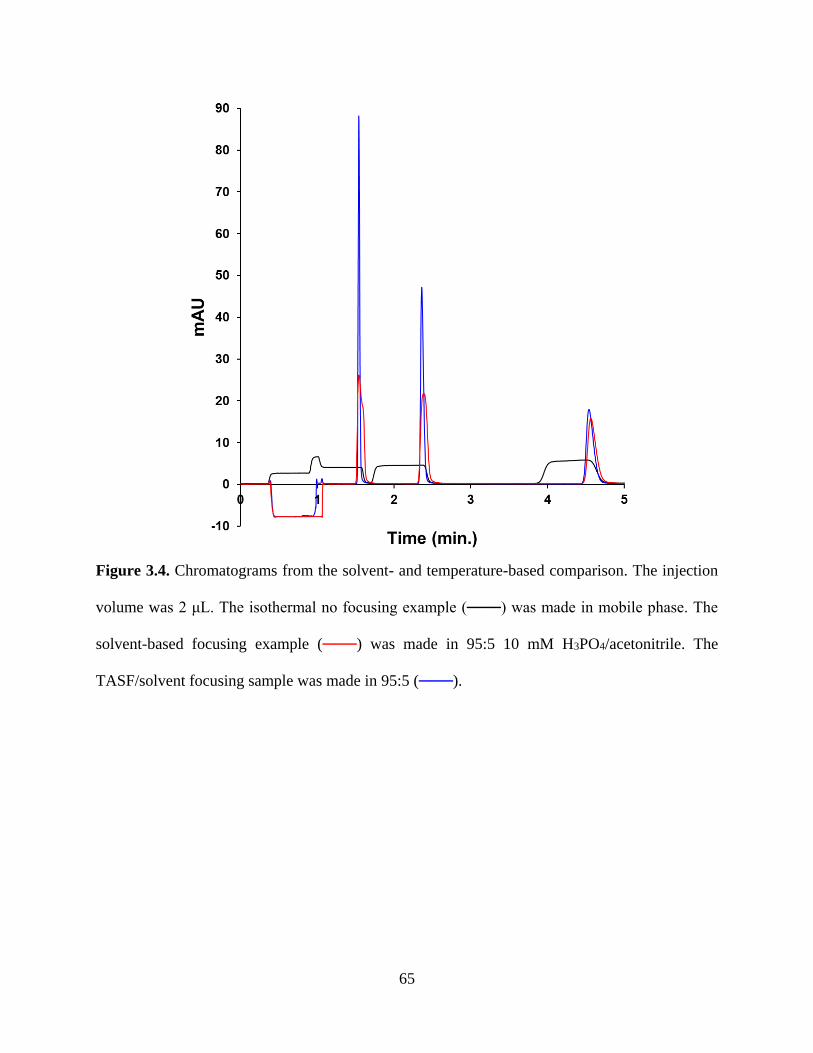
65

Figure 3.4. Chromatograms from the solvent- and temperature-based comparison. The injection

volume was 2 μL. The isothermal no focusing example (───) was made in mobile phase. The

solvent-based focusing example (───) was made in 95:5 10 mM H3PO4/acetonitrile. The

TASF/solvent focusing sample was made in 95:5 (───).

66

3.3.5 TASF increases sensitivity for samples made in strong elution solvent

The problem of peptide adsorption to containers and other surfaces during analysis is a serious one

[101]. Very frequently, a solution of a peptide prepared in an acidic organic/aqueous mixture yields

less adsorption than purely aqueous solvents [14, 101-106]. While adsorption may occur within

the LC instrument itself [102], here we are concerned with the stability of the solution prior to

injection. Maes et al. [102] found that an acidic water/AN (87:13 v/v) solvent was best for a set of

neuropeptides. Earlier, Vatansever et al. noted that acidic AN/water solvents were best for a series

of peptides but the optimal concentration of acetonitrile, which was as high as 30%, depended on

the peptide [103]. Amyloid peptides are best handled in basic water/AN 80:20 [104, 105], while

calcitonin is stable in water/AN (43:57). Thus, very often analytical determinations of peptides

must be carried out with a sample in a solvent with significant elution strength.

We have an interest in the peptide galanin and the products of its hydrolysis in the extracellular

space of hippocampal tissue cultures [107, 108]. Our experimental protocol involves the use of

electroosmotic flow to perfuse an organotypic hippocampal slice culture with a peptide at high

(~300 μM) concentration and variable but low (10 - 25 nL/minute) flow rate. Over a 5-minute

sampling time, we collect 50 – 125 nL of the perfusion solution containing peptide and hydrolysis

products. This volume is diluted to 10 or 15 μL depending on the application [107-109]. The final

concentration of galanin in the injected samples is a few micromolar. Zhou et al. [14] have found

that galanin is most stable in an W/AN 80:20 solution. In this example the elution strength of the

sample matrix is fixed at this composition and stronger than the 85:15 0.1% TFA/AN mobile

phase. In principle, the sample could be diluted with water or an aqueous solution, however the

point of using the acetonitrile-based solvent is to avoid losses by adsorption. Thus, dilution with

an aqueous solution would be counterproductive.

67

TASF, on the other hand, should be capable of concentrating the injected peptide despite its

relatively high organic content. Figure 3.5 shows the results for isothermal (black) and TASF

(blue) separations of a 500 nL injection of 100 nM galanin dissolved in 80:20 W/AN onto a 250

nL volume column. Sensitivity is important to our galanin application. Thus we have selected a

sample concentration to clearly demonstrate the potential for TASF-induced improvements in

preconcentration. The red dashed line in Figure 3.6 indicates the detector’s limit of quantitation

calculated for an absorbance value required to be a factor of ten greater than the standard deviation

of the baseline noise. The isothermal column temperature was 65 °C and the focusing temperature

was -10 °C. Clearly, TASF improves preconcentration and detection limits for trace level peptide

samples made in strong elution solvents.

68

Figure 3.5. Chromatograms resulting from the application of TASF to increasing analysis

sensitivity for the peptide galanin. Galanin samples were made in 80:20 water/acetonitrile and 500

nL samples were injected onto a 250 nL volume column operated with a mobile phase composition

of 85:15 0.1% TFA/acetonitrile. Isothermal (───) column temperature was 65 °C. TASF (───).

The red dashed line represents the detectors limit of quantitation. With a focusing temperature set

to -10 °C peak height increased by a factor of 3, relative to an isothermal analysis.

69

3.4 CONCLUSIONS

This work demonstrates the utility of temperature-based on-column solute focusing to improve

peak shape in capillary LC. We can draw the following conclusions:

1. Dispersion and the increase in apparent void time induced by the pre-column void

necessary for effective implementation of TASF can be significantly reduced by packing

the void with solid non interacting silica spheres.

2. The TASF system is robust; it can be easily incorporated into a modern automated

instrument. It is capable of unattended operation for extend periods.

3. The combination of TASF with solvent-based focusing is very effective. The two focusing

techniques are complementary, improving peak shape and analysis sensitivity for large

volume samples.

4. TASF has the potential to focus large-volume samples made in solvents with elution

strength greater than that of the mobile phase.

These results illustrate the potential of temperature to be used as an effective tool to enhance

overall separation performance. They clearly demonstrate that TASF can be used independently

or in conjunction with solvent-based on-column focusing to enhance analysis sensitivity and

separation efficiency in capillary liquid chromatography.

70

4.0 QUANTITATIVE EVALUATION OF MODELS FOR SOLVENT-BASED

ON-COLUMN FOCUSING IN LIQUID CHROMATOGRAPHY




4.1 INTRODUCTION

In most analytical chromatographic analyses, the injected volume of sample is much smaller than

the volume of mobile phase carrying a peak out of the column (the peak volume). In this case, the

amount of sample injected affects the peak height linearly, but has no effect on the peak width. If

the volume of sample injected is increased to enhance concentration detection limits, at some point

the eluting peak will become broadened. This phenomenon is now termed volume overload. It is

worth noting that a very accurate picture of this phenomenon was published in 1956 by van

Deemter et al. using gas chromatography [3]. Sternberg later put this effect into rigorous

mathematical terms by explaining that volume overload leads to a peak shape that is a convolution

of the peak shape observed with a small-volume injection and the rectangular concentration-

distance profile as injected [110]. The former can be determined from a small-volume injection.

The latter comes from the fact that the length of the zone of solute on the column once the injection

is complete is smaller by the factor 1 (1 + 𝑘′) ⁄ than the length of the column occupied by the

injected solvent. Further, Sternberg pointed out that the variance of the resulting peak was the sum

of the variances of the two functions. It becomes a simple matter to calculate the maximum injected

71

volume that leads to an acceptable increase in peak width. Injecting this volume will lead to the

highest concentration sensitivity with minimal (tolerable) impact on separation quality.

When the sample liquid is a weaker chromatographic solvent than the mobile phase, analyte

retention on the stationary phase is higher, increasing the allowable injected volume in comparison

to the allowable volume when the sample liquid is the mobile phase. This phenomenon, often

called on-column focusing or preconcentration, is used routinely in capillary LC (cLC) where the

injection of low nL-scale volumes is required to avoid volume overload when injecting samples

made in mobile phase [23-25, 63]. On-column focusing is not limited to cLC, it can be used to

advantage with any size column [95, 111] or application from trace analysis to two-dimensional

LC [112-118]. On-column focusing also happens quite often as a natural consequence of gradient

elution chromatography because many solutes are highly retained in the relatively weak initial

solvent composition as described by Snyder [119]. He described an additional effect that occurs in

gradient elution, namely, the peak compression of the already focused band that results because

the tail of the injected band moves with the stronger solvent for a longer time than the front of the

band. As our current interest is in isocratic elution with on-column focusing followed by peak

compression due to the introduction of the stronger mobile phase, we will discuss the problem in

the context of a step gradient. Thus, there are two factors to consider in solvent-based on-column

focusing: one relates to the retention factor of the solute as it is injected and the other is due to the

compression occurring when the mobile phase is stronger than the injected sample’s liquid. In the

following discussion, we do not consider the case where mass overload contributes to

bandspreading.

Several groups have contributed to the understanding of these phenomena. Snyder’s work has been

mentioned [21, 22]. Later, the Poppe group combined the on-column focusing and the step-

72

gradient-induced compression in the context of a precolumn trapping column/backflush for

analytical work [120, 121]. They arrived at the simple result that the solute elutes from the column

in a volume that is a factor 𝑘2 𝑘1 ⁄ smaller than the injected volume, where 𝑘1 is the solute retention

factor in the sample solvent and 𝑘2 is the retention factor in the mobile phase. Here, for simplicity

column dynamics-induced bandspreading was ignored. Hartwick, and subsequently the Desmet

group found the same relationship for post-column peak trapping/concentration and elution [122-

124]. The same relationship was found for preconcentration in CEC [125].

Mills et al. [48] also derived a factor for preconcentration resulting from the step gradient using a

vaguely described function of 𝑘1 and 𝑘2 in Slais et al. [61]. Rather than finding the factor 𝑘2 𝑘1 ⁄

they found the factor (1+𝑘2

1+𝑘1)

2. This predicts rather large focusing effects. For instance, if 𝑘1 = 50

and 𝑘2 = 5, the former relationship predicts that the eluted volume would be 10 times smaller than

the injected volume while Mills et al.’s relationship predicts that the eluted volume would be 72

times smaller than the injected volume.

Unfortunately, no quantitative evaluation of these relationships exists. The rationale for focusing

is to increase sensitivity, so a natural quantitative test is to determine the sensitivity enhancement

from these processes. Numerically, the sensitivity enhancement is the inverse of the ratios

discussed in the last paragraph. However, peak height is strongly influenced by on-column

bandspreading which depends on numerous phenomena. As a result, predicted sensitivity

enhancements that do not take into account on-column dynamic bandspreading will be optimistic

so they cannot themselves form the basis for a quantitative evaluation of a model. Another

approach to testing these predictions is to calculate a volume that can be injected without

significant volume overload and then test this experimentally. This approach requires a knowledge

73

of the number of theoretical plates, N, experienced by each solute in the absence of volume

overload, a knowledge of the shape of the injected volume (in order to estimate its variance

contribution to the overall peak variance), as well as a quantitative assertion of the fractional loss

in N that the chromatographer is willing to accept. Because of these factors, this approach also

cannot quantitatively confirm the expected result despite its significant practical significance.

In this work, we first recapitulate the simple theoretical derivation of the 𝑘2 𝑘1 ⁄ focusing factor.

As described above, there are several extant publications reciting the same result. However, it is

important to show clearly how this result occurs as a part of this discussion. We have designed an

experiment in which we attempt to experimentally validate this relationship by measuring peak

width rather than peak height. As the objective is to determine accurately the ratio of eluted volume

to injected volume, we create eluted volumes significantly greater than the natural peak volume.

This is in contrast to the work cited above where the objective was to demonstrate the utility of

on-column focusing to enhance sensitivity in analytical determinations, not the validity of the

model. Using accurately determined experimental retention factors and measurements of the

injection band width we comment on the validity of the 𝑘2 𝑘1 ⁄ factor and its practical application

to increase analysis sensitivity in liquid chromatography.

4.2 THEORY

4.2.1 Derivation of the 𝒌𝟐 𝒌𝟏 ⁄ factor

Consider a zone of solute of volume Vinj injected into a column. During the injection the relative

volumes of the sample and the column suffice to cause the sample liquid itself to be the mobile

phase transiently during sample loading. The discussion that follows will consider the on-column

length occupied by the injected volume. Figure 4.1 illustrates the process schematically. At t = 0

74

a volume Vinj passes from the loop onto the column. The solute will occupy a length ℓ1on the

column given by Eq. 4.1 in which the injection time, 𝑡𝑖𝑛𝑗 is multiplied by the average zone velocity.

The former is Vinj/F where F is flow rate, while the latter is the determined by the average mobile

phase velocity vmp and k1 the retention factor for the solute in the sample liquid acting as mobile

phase.

ℓ1 = (𝑉𝑖𝑛𝑗

𝐹)

𝑣𝑚𝑝

1 + 𝑘1 = 𝑡𝑖𝑛𝑗

𝑣𝑚𝑝

1 + 𝑘1

(4.1)

As the mobile phase passes through the sample band the step gradient that follows compresses the

zone further. Additional compression results because the stronger elution strength mobile phase

moves the tail of the zone for a longer time than it moves the front. We will thus determine how

far the tail of the zone moves, Δℓ𝑡, and how far the front of the zone moves, Δℓ𝑓, in the time that

it takes for the mobile phase to reach the front of the zone, t1. Once the mobile phase reaches the

front of the zone, there is no further compression by the step gradient. The time, t1, that the mobile

phase requires to reach the moving front of the zone is given by a distance into the column, ℓ2,

and the velocity vmp. The distance ℓ2 (Figure 4.1) is the initial length of the compressed zone plus

the additional distance moved at the front,

ℓ2 = 𝑡1𝑣𝑚𝑝 = ℓ1 + ∆ℓ𝑓

(4.2)

During time t1, the front moves at a velocity vmp/(1+k1). The distance the front moves in time t1 is:

75

∆ℓ𝑓 = 𝑡1

𝑣𝑚𝑝

1 + 𝑘1

(4.3)

Replacing ℓ1 in Eq. 4.2 with Eq. 4.1 and Δℓ𝑓 with Eq. 4.3 and rearranging leads to Eq. 4.4.

𝑡1 =𝑡𝑖𝑛𝑗

𝑘1

(4.4)

Figure 4.1. Schematic describing the effect of solvent-based on-column focusing. Compression of

the injection zone results from the increased retention at the head of the column in the sample

solvent and the step-gradient resulting from the higher elution strength mobile phase passing

through the injection plug.

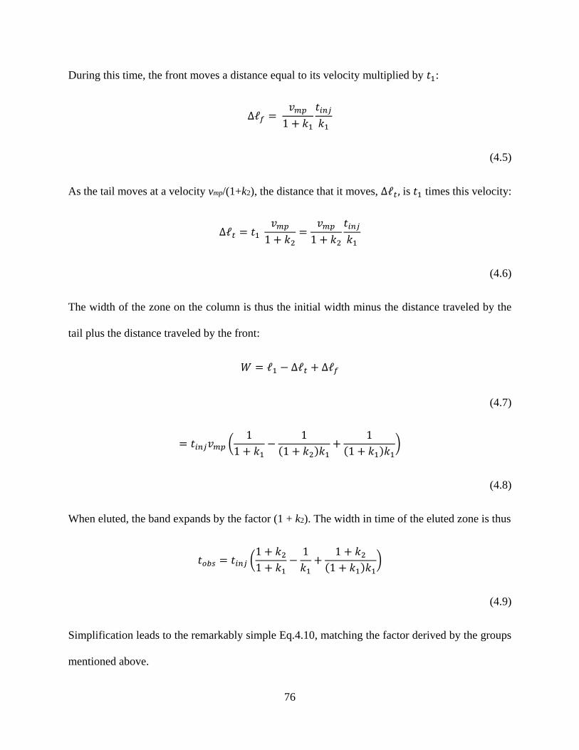
76

During this time, the front moves a distance equal to its velocity multiplied by 𝑡1:

∆ℓ𝑓 = 𝑣𝑚𝑝

1 + 𝑘1

𝑡𝑖𝑛𝑗

𝑘1

(4.5)

As the tail moves at a velocity vmp/(1+k2), the distance that it moves, ∆ℓ𝑡 , is 𝑡1 times this velocity:

∆ℓ𝑡 = 𝑡1 𝑣𝑚𝑝

1 + 𝑘2=

𝑣𝑚𝑝

1 + 𝑘2

𝑡𝑖𝑛𝑗

𝑘1

(4.6)

The width of the zone on the column is thus the initial width minus the distance traveled by the

tail plus the distance traveled by the front:

𝑊 = ℓ1 − ∆ℓ𝑡 + ∆ℓ𝑓

(4.7)

= 𝑡𝑖𝑛𝑗𝑣𝑚𝑝 (1

1 + 𝑘1−

1

(1 + 𝑘2)𝑘1+

1

(1 + 𝑘1)𝑘1)

(4.8)

When eluted, the band expands by the factor (1 + k2). The width in time of the eluted zone is thus

𝑡𝑜𝑏𝑠 = 𝑡𝑖𝑛𝑗 (1 + 𝑘2

1 + 𝑘1−

1

𝑘1+

1 + 𝑘2

(1 + 𝑘1)𝑘1)

(4.9)

Simplification leads to the remarkably simple Eq.4.10, matching the factor derived by the groups

mentioned above.

77

𝑡𝑜𝑏𝑠 = 𝑡𝑖𝑛𝑗

𝑘2

𝑘1

(4.10)

We can break Eq. 4.10 down into two components, one from the initial focusing of the injected

zone as shown in Eq. 4.1 and one from the compression that results. In the absence of this

compression effect, the on-column width of the injected solute zone is given by Eq. 4.1. That on-

column width remains unchanged in this compression-free model. Of course, bandspreading

occurs, but here we just consider the volume overload portion of the problem. In addition, as

explained below in Section 4.2.2, the zone width is somewhat independent of mass-transport-based

bandspreading. When the zone is eluted, its width in time units, 𝑡𝑜𝑏𝑠, is the length, ℓ1, divided by

the velocity which is now dependent on 𝑘2.

𝑡𝑜𝑏𝑠 = 𝑡𝑖𝑛𝑗

𝑣𝑚𝑝

1 + 𝑘1

1 + 𝑘2

𝑣𝑚𝑝= 𝑡𝑖𝑛𝑗

1 + 𝑘2

1 + 𝑘1

(4.11)

By comparison of Eqs. 4.10 and 4.11, it can be seen that the effect of compression alone is

𝑘2

𝑘1

1 + 𝑘1

1 + 𝑘2

(4.12)

In summary, the width in time of the eluted zone resulting from an injection large enough to create

obvious volume overload is expected to be the factor 𝑘2 𝑘1⁄ times the injection time. This factor

is the product of two factors. One is the initial band focusing due to retention of the solute in the

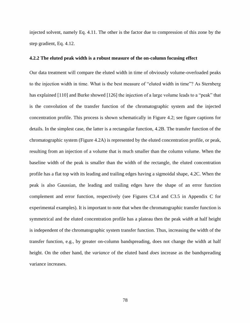
78

injected solvent, namely Eq. 4.11. The other is the factor due to compression of this zone by the

step gradient, Eq. 4.12.

4.2.2 The eluted peak width is a robust measure of the on-column focusing effect

Our data treatment will compare the eluted width in time of obviously volume-overloaded peaks

to the injection width in time. What is the best measure of “eluted width in time”? As Sternberg

has explained [110] and Burke showed [126] the injection of a large volume leads to a “peak” that

is the convolution of the transfer function of the chromatographic system and the injected

concentration profile. This process is shown schematically in Figure 4.2; see figure captions for

details. In the simplest case, the latter is a rectangular function, 4.2B. The transfer function of the

chromatographic system (Figure 4.2A) is represented by the eluted concentration profile, or peak,

resulting from an injection of a volume that is much smaller than the column volume. When the

baseline width of the peak is smaller than the width of the rectangle, the eluted concentration

profile has a flat top with its leading and trailing edges having a sigmoidal shape, 4.2C. When the

peak is also Gaussian, the leading and trailing edges have the shape of an error function

complement and error function, respectively (see Figures C3.4 and C3.5 in Appendix C for

experimental examples). It is important to note that when the chromatographic transfer function is

symmetrical and the eluted concentration profile has a plateau then the peak width at half height

is independent of the chromatographic system transfer function. Thus, increasing the width of the

transfer function, e.g., by greater on-column bandspreading, does not change the width at half

height. On the other hand, the variance of the eluted band does increase as the bandspreading

variance increases.

79

Figure 4.2. Simulated signals for the eluted injection profile corresponding to the convolution of

the column transfer function and rectangular injection profile. Panel A shows an exponentially

modified Gaussian signal resulting from on-column bandspreading (σ = 0.75 s, 𝜏 = 1 s, α5% = 2.8);

panel B a 15 s wide rectangular injection profile. Panel C shows the peak shape resulting from the

convolution of the signals in panels A and B in blue. The black dashed trace is used to overlay the

15 s wide injection profile on the convolved signal illustrating the potential utility of the half width

metric to quantitatively evaluate the on-column focusing effect.

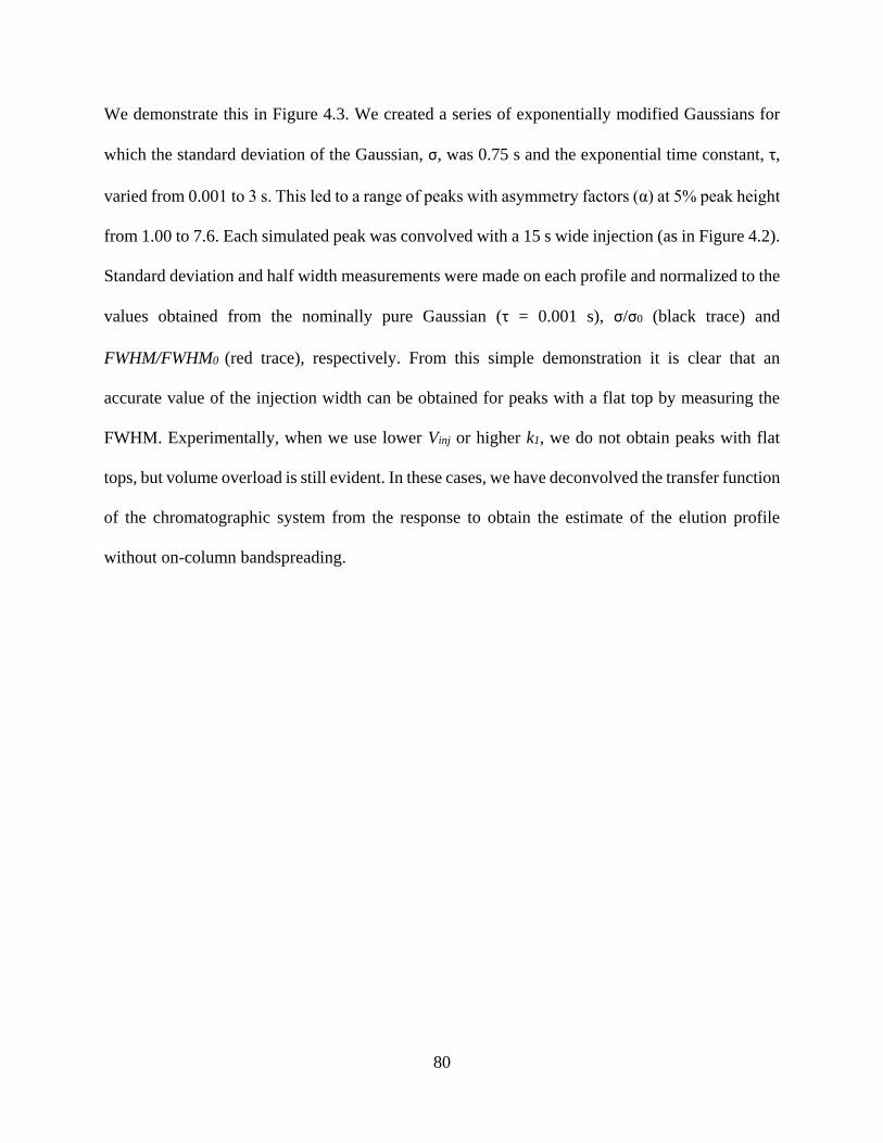
80

We demonstrate this in Figure 4.3. We created a series of exponentially modified Gaussians for

which the standard deviation of the Gaussian, σ, was 0.75 s and the exponential time constant, τ,

varied from 0.001 to 3 s. This led to a range of peaks with asymmetry factors (α) at 5% peak height

from 1.00 to 7.6. Each simulated peak was convolved with a 15 s wide injection (as in Figure 4.2).

Standard deviation and half width measurements were made on each profile and normalized to the

values obtained from the nominally pure Gaussian (τ = 0.001 s), σ/σ0 (black trace) and

FWHM/FWHM0 (red trace), respectively. From this simple demonstration it is clear that an

accurate value of the injection width can be obtained for peaks with a flat top by measuring the

FWHM. Experimentally, when we use lower Vinj or higher k1, we do not obtain peaks with flat

tops, but volume overload is still evident. In these cases, we have deconvolved the transfer function

of the chromatographic system from the response to obtain the estimate of the elution profile

without on-column bandspreading.

81

Figure 4.3. Influence of peak asymmetry on peak variance and half width for a series on

exponentially modified Gaussians simulated using σ = 0.75 s, 𝜏 = 0.001 to 3 s, α5% = 1.00 to 7.6.

Each Gaussian signal was convolved with a 15 s wide injection plug. Peak variances were

calculated using the method of moments, half width measurements were made on each profile and

each was normalized to the values obtained from the untailed Gaussian injection. The black trace

shows the strong influence of peak tailing on the calculated band variance. The red trace highlights

the rather small influence of peak tailing on the bands width at half height.

82

4.3 INSTRUMENTATION AND CHROMATOGRAPHGIC CONDITIONS

4.3.1 Chemicals

Methyl, ethyl, and n-propyl esters of p-hydroxybenzoate (parabens, notated here after as PB1, PB2,

and PB3, respectively) and uracil were purchased from Sigma-Aldrich (St. Louis, MO). Standard

solutions for parabens were made by dissolving each individually in acetonitrile. Uracil stocks

were made in deionized water. Water was from a Millipore Milli-Q Synthesis A10 water

purification system (Billerica, MA) and used without further treatment. Acetonitrile (LC/MS

Optima grade), isopropanol (HPLC grade), acetone (HPLC grade) and phosphoric acid (HPLC

grade) were from Fisher Scientific (Fair Lawn, NJ)

4.3.2 Instrumentation

Figure 4.4 shows a simple schematic for the instrumentation used. Waters 1.7 μm dp Acquity BEH

C18 particles (Milford, MA) were packed in-house into 150 µm ID x 360 µm OD fused-silica

capillaries from Polymicro Technologies (Phoenix, AZ). Column length was 5.5 cm. The

remainder of the column was packed with 8 µm solid silica spheres (Thermo). To determine the

extra column time a nominally identical fused-silica capillary was packed with 8 µm solid silica

spheres. We refer to this column as the e-column. For complete details related to column

preparation see section C3.1 of Appendix C. The columns packed with stationary phase and 8 µm

silica spheres (A) and the e-column (B) were connected directly to a 6-port Cheminert injection

valve (C72-6676EH, VICI Valco, Houston, TX) using 1/16” OD x 0.015” ID PEEK sleeves

(IDEX-Health and Science, Oak Harbor, WA). The additional 3.9 cm segment of each column

allowed the unheated, room temperature segment of capillary (2.4 cm) located within the injection

valve not to adversely influence the solute retention. In addition, 1.5 cm of the capillary served as

83

a mobile phase pre-heater. A 75 cm x 75 µm ID nanoViper capillary (volume = 3.3 µL, Thermo)

was used as the sample loop. An Ultimate 3000 RSLCnano high pressure gradient pump (NCP-

3200, Thermo, Germering, Germany) was used to deliver mobile phase. Detection was achieved

using a Waters Acquity TUV detector equipped with a 10 nL flow cell (Waters) set to 254 nm.

The column outlet and flow cell were connected by a 30 cm x 25 µm ID fused-silica detection

capillary (Polymicro). Data acquisition and export were achieved by connecting the Acquity TUV

analog output to an Agilent 1200 UIB (G1390B, Agilent Technologies, Waldbronn, Germany) and

Agilent OpenLab ChemStation CDS software (rev. C01.06). Valve actuation was controlled by a

National Instruments USB-6008 DAQ and a simple LabVIEW routine written in-house (rev. 2014,

National Instruments, Austin, TX). Column temperature was controlled using a simple homemade

resistive heating assembly previously described [92, 99]. Further details regarding instrument

configuration and control are provided in Appendix C.

Figure 4.4. Diagram for the instrumentation used in this work. Two-segment capillary columns

(A) consisting of non-interacting silica spheres and stationary phase were attached directly to the

injection valve and placed inside a resistively heated insulated enclosure. To accurately determine

84

the extra-column contributions to t0 injections were made into a so-called e-column (B). The e-

column consisted of all portions of the two-segment column except the stationary phase.

4.3.3 Chromatographic conditions

Precise details related to the preparation of eluents and sample solutions used in this study are

critical to interpretation of results. As a result, all samples and eluents were prepared

gravimetrically in batches large enough to minimize irregularities in sample preparation and

absolute mobile phase composition. Mobile phase was prepared by mixing acetonitrile and 10.0

mM H3PO4 in water at 5.0, 10.0, and 20.0% (wt%). The 5.0 and 20.0% acetonitrile mobile phases

were made in 1.000 kg batches; the 10.0% solvent was prepared at the 0.500 kg scale. Mobile

phase was degassed and filtered using 0.45 µm nylon membrane filters (Millipore) prior to use.

Paraben retention studies used 50 nL timed injections of 250 µM uracil, PB1, PB2, PB3 samples

made in each mobile phase. Care was taken to maximize peak height by injecting the highest

concentration sample without mass overloading the column. Stock solutions employed for

retention studies were made at 200 mM in acetonitrile. Spikes, 125 µL, from each stock were made

into 100.0 g volumes of premixed mobile phase to achieve desired solute concentration. For

retention studies, differences between sample and mobile phase composition were kept less than

0.5%. This small composition difference was due to the additional acetonitrile present in the

sample, from the three 125 µL paraben spikes.

Solvent-based focusing studies used large-volume, timed injections corresponding to 500, 1000,

1500, and 2000 nL. Samples were made using 100.0 g portions of the appropriate premixed mobile

phase described above. Paraben concentrations were 10 µM each. Samples were prepared from 50

85

mM stock solutions made in acetonitrile (20 µL spikes). Thus, differences between sample and

eluent composition were less than 0.1%.

The premixed mobile phase for retention and injection volume studies, 80:20 10.0 mM

H3PO4/acetonitrile (wt%), was used as both solvent A and solvent B in the Ultimate 3000 pump.

The flow rate was 4.00 µL/min with eluent composition set to 50:50 channel A/B. Column

temperature was maintained at 60.0 ± 0.1 ºC. All retention studies used samples whose

composition was nominally identical to the mobile phase and retention measurements were made

with n = 4. Focusing studies were performed in duplicate and used samples made in 95:5, 90:10,

and 80:20 10 mM H3PO4/acetonitrile (wt%) with mobile phase composition maintained at 80:20

10 mM H3PO4/acetonitrile (wt%).


4.4.1 Accurate determination of solute retention factors

To assess the validity of each focusing model we need accurate retention factors. Mobile phase

composition and solutes were selected based on our experience to provide a range of k’ values that

would be a good test for the models. Table 4.1 shows the values of k’ determined from solute

retention time at the peak maxima for three mobile phase compositions (80.0:20.0, 90.0:10.0,

95.0:5.0 (wt%)) at 60.0 °C for the three solutes PB1, PB2, PB3. PB3 was omitted from the 5.0%

acetonitrile sample due to excessive retention. Retention factors were calculated using Eq. C3.1

with n = 4. Retention factors were also calculated based on first central moments for uracil and

each paraben (see section C3.4 of Appendix C). No significant difference in focusing results were

obtained using either method.

86

Table 4.1. Experimentally determined retention factors for methylparaben, ethylparaben and

propylparaben.

ϕ 0.20 0.10 0.05

Solute 𝒌′ σk 𝒌′ σk' 𝒌′ σk

PB1 2.06 0.017 7.02 0.019 18.75 0.05

PB2 4.62 0.04 19.62 0.05 59.3 0.19

PB3 10.82 0.08 57.6 0.2 - -

We note here that evaluation of the models requires accurate measurement of the extent of

focusing. This means that injected bands must not be too well-focused or else the natural

bandspreading processes will lead to a peak variance that is much larger than the variance of the

injected rectangular width. The range of k1 and k2 values shown in Table 4.1 reflects this. As we

are using capillary liquid chromatography, extra-column volume can be a significant fraction of,

or even exceed, the column volume. We paid particular attention to determining accurate values

of t0 and solute retention times, tR (see Appendix C for details), in order to determine accurate

values of k1 and k2.

4.4.2 System performance evaluation

As a check on system performance, we performed two control experiments for which the outcome

was reliably predictable. In one, a series of timed injections of uracil were made into a 25 µm ID

87

empty tube. As Figure C3.4 shows, a plot of the full-width of the rectangular zones (in time units)

vs. the injection time is linear. From the slope we can calculate the volumetric flow rate (Eq. C3.2).

Flow rate calculated from the data in Figure C3.4 was 3.977 ± 0.030 µL/minute. In the second

control experiment, a sample of PB1, PB2, and PB3 was prepared in the mobile phase (80:20

(wt%) phosphate/acetonitrile). Injections from 250 to 1500 nL gave wide eluted zones. Plots of

the full-width of the observed zone in units of time vs. the injection time give a slope of 0.992 ±

0.006 and an intercept of -0.008 ± 0.002 (means and 95% confidence intervals, Figure C3.5). Full

details for performance evaluation experiments are provided in sections C3.4 and C3.5 of

Appendix C. We can conclude from results of both control experiments that system performance

is satisfactory for the current work.

4.4.3 Quantitative evaluation of solvent-based focusing

4.4.3.1 Solvent-based on-column focusing examples

We made injections of 10.0% (wt%) acetonitrile containing samples of PB1, PB2, and PB3 with

Vinj = 500 to 2000 nL into a column with 20.0% acetonitrile as the mobile phase. Figure 4.5 shows

two example chromatograms in which a small amount of focusing is expected to occur as the

composition of the injected solution is weaker than the mobile phase (the full data set is Figure

C3.6). Injection volumes for the black and blue traces were 500 and 1500 nL. Qualitatively it is

clearly apparent from Figure 4.5 that the 1500 nL injection leads to a volume overloaded peak for

PB1 and PB2. Low-retention solutes, particularly PB1 in this demonstration, are most susceptible

to volume overload. Under the conditions evaluated, PB1 and PB2 retention factors in the sample

solvent and eluent were k1 = 7.02 and 19.62 with k2 = 2.06 and 4.62. These factors do not lead to

a Gaussian peak shape for the 1500 nL injection.

88

Figure 4.5. Example chromatograms resulting from 500 nL (black) and 1500 nL (blue) injections

of paraben samples made in 90:10 wt% 10 mM H3PO4/acetonitrile. In each of the two

chromatograms, the peaks correspond (in the order of elution) to PB1, PB2, and PB3; mobile phase

consisted of 80:20 wt% 10 mM H3PO4/acetonitrile. Negative peaks are caused by the injection

solvent’s refractive index being different from that of the mobile phase. For chromatographic

conditions see Section 4.3.3.

89

Figure 4.6 shows the results for the full range of injection volumes for each solute under all

focusing conditions evaluated. Panels A, B and C correspond to PB1, PB2, and PB3 in 10.0%

(wt%) acetonitrile. Panels D, E, and F show PB1, PB2, and PB3 in 5.0% (wt%) acetonitrile. After

correcting the time axis for the injection time so that the fronts of all zones for a particular solute

overlap it can be seen that the peaks get wider as the injection volume increases from 500 to 2000

nL for all solutes. For comparison, a 50 nL injection of 250 μM PB1, PB2, and PB3, 5.0% and

10.0 (wt%) acetonitrile, is shown in each panel as a dashed gray line. The relative effect of the

injection width on the peak width, as expected, is smaller for the higher k’ compound PB3 than

the others. Peak width for each solute in panels D, E, and F is narrower than its analogous injection

in panels A, B, and C, as expected, because of the larger values of 𝑘1 in the 5% acetonitrile sample

(see Table 4.1). Note that the PB1 and PB2 peaks in panels D and E still exhibit some signs of

volume overload for the largest injection volumes, however the peak widths for PB3 in panel F

are constant, varying between 3.1 and 3.3 s across the injection volume range tested (50 nL to 2000

nL). The lack of volume overload for the PB3 peak demonstrates the analytical effectiveness of

focusing, but as described above does not help to establish the validity of a quantitative model.

As described above, for clearly volume overloaded peaks with flat tops the simple FWHM

measurements can be used to evaluate focusing accurately. When on-column focusing is

significant as for PB2 and PB3 in panels E and F, deconvolution will be used to remove the

contribution from on-column and post-column processes allowing us to determine the width of the

injection profile. In cases such as the just-described PB3 peaks, volume overload has virtually no

effect on peak width so deconvolution cannot reveal its magnitude.

90

Figure 4.6. Time adjusted chromatograms for 500 (black), 1000 (red), 1500 (blue), and 2000

(purple) nL injections of paraben samples made in 90:10 wt% (A-C) and 95:5 wt% (D-F) 10 mM

H3PO4/acetonitrile; mobile phase consisted of 80:20 wt% 10 mM H3PO4/acetonitrile. Panels A and

D correspond to PB1; B and E to PB2, and C and F to PB3. The time axes for each large volume

injection were aligned to the leading edge of each injection profile. Analogous 50 nL injections

for each solute (- - -) are also provided in each panel. For additional chromatographic conditions

see Section 4.3.3. Complete chromatograms for each injection are provided in Figures C3.7 and

C3.8.

91

4.4.3.2 Quantitative comparison of focusing models

Figure 4.7 is a plot of the expected benefit from solvent-based preconcentration for three cases as

a function of the single variable 𝑘2 𝑘1 ⁄ . The three cases are (red) focusing and compression (Eq.

4.10), the effect of focusing alone (Eq. 4.11, gray), and the prediction of Mills et al. ( lavender).

The latter two are ranges because neither effect can be expressed as a function of 𝑘2 𝑘1 ⁄ only.

Thus, the effect at a given value of 𝑘2 𝑘1 ⁄ depends on the actual values (magnitude) of each of the

two retention factors. Of course, the prediction for Eq. 4.10 is a straight line. The general

conclusions are that the step-gradient-induced compression, while small when considering peak

capacity in gradient elution [21, 22, 119, 127] is nonetheless significant when considered from the

perspective of sensitivity. In addition, for low values of 𝑘2 𝑘1 ⁄ , which would be the normal case

in practice, the Mills et al. theory predicts dramatically better preconcentration than Eq. 4.10.

With accurate values for k1 and k2 for each solute and condition, we can calculate the expected

effect from each case as shown in Figure 4.8 which, as Figure 4.7 shows Eq. 4.10 (red), Eq. 4.11

(black) and Mills et al. (blue). Several things are clear. (1) The data describe, within experimental

error, a straight line. This supports the idea that Eq. 4.10 most adequately predicts the combined

effects of focusing and compression. The experimental slope is 0.90 which is significantly different

than the predicted slope, 1.0. We discuss this below. (2) The prediction of the oft-cited work by

Mills et al. is not at all accurate. We do not believe that there is justification for using this model

to estimate the allowable volume injected or the achievable sensitivity enhancement. (3) As Snyder

points out [127] the effect of compression is small, but it is by no means negligible as Figure 4.8

shows by comparing the black and red points for individual k2/k1 combinations.

92

Figure 4.7. Simulations for the apparent on-column focusing (tobs/tinj) resulting from each model

were calculated as a function of k2/k1. Retention factors were varied from 1 < k1 < 500 and 1 < k2

< 20; tobs/tinj was calculated for every combination of k2/k1 within this range. The lavender and gray

bands represent the range of tobs/tinj values obtained when varying the ratio of k2/k1 based on the

model derived by Mills et al. and Eq. 4.11, respectively. The red line represents the calculated

tobs/tinj based on the k2/k1 model incorporating the effect of the step gradient. Note that for each of

the values of k1 and k2 simulated using the k2/k1 model only a single value for tobs/tinj is obtained

regardless of the magnitude of k1 and k2, i.e. only the ratio of k2/k1 matters; this is not predicted by

the other two models. As expected all three models for on-column focusing converge at both

corners of the plot where no focusing and large amounts of focusing are present.

93

There are several factors that may contribute to the observed deviation from the very simple model.

Among the factors to consider are whether values of k’ at constant temperature are accurate,

whether temperature control is adequate, and whether pressure changes alter the picture. We have

made extensive efforts to account for the potential influence of these parameters on the results

presented in Figure 4.8. Sections C3.2, C3.3, and C3.4 of Appendix C address potential

inaccuracies in k’ values. Temperature irregularities on the order of a few degrees, either in the

form of viscous heating or local temperature variations in the column heating element could not

account for the magnitude of the extra compression observed. The high thermal conductivity of

fused silica columns as well as operating them under the moderate linear velocities used here are

also not likely to induce viscous heating related changes in k’ [100]. Pressurizing the sample in

the loop will reduce its volume and thus reduce the initial zone width. The pump pressurizes the

loop contents to 425 bar. Sample volume will be decreased less than 2% under these conditions

[88]. Thus, it is unlikely that pressure-based compression of the sample either in the loop or at the

head of the column can account for the extra compression.

94

Figure 4.8. Quantitative comparison of on-column focusing models. Experimental data based on

deconvoluted injection width measurements and retention factors in Table 4.1 are plotted as red

circles. Data points correspond to replicate injections of: 1000, 1500, 2000, and 1500 and 2000 nL

injections of methylparaben made in 90:10 and 95:5 wt% 10 mM H3PO4/acetonitrile, 1500, 2000,

and 2000 nL injections of ethylparaben in 90:10 and 95:5 wt% 10 mM H3PO4/acetonitrile, and

2000 nL injections of propylparaben in 90:10 wt% 10 mM H3PO4/acetonitrile. A total of 18 data

points are plotted corresponding to 5 different k2/k1 ratios. The solid red line corresponds to the

degree of focusing predicted by the k2/k1 model and experimental k’ values. Bands calculated based

on Eq. 4.11 and the Mills model for the range of k1 and k2 values encompassed by the experimental

range (see Table 4.1) are plotted as gray and lavender bands, respectively. Individual points based

on each experimental k1 and k2 value are also plotted for these two models and shown as black and

blue circles.

95

One factor that may explain the extra compression is the actual solvent composition profile on the

column when the mobile phase returns to the column behind the injected volume. Consider the

simple case in which the solvent front enters the column as a sharp front but spreads as it proceeds

down the column. The spreading may be caused by column mass transport dynamics or it may be

caused by depletion of organic modifier in the mobile phase at the solvent front as the amount of

adsorbed organic modifier increases to equilibrate with the new, modifier-rich mobile phase.

Recall that the on-column compression is caused by the fact that the tail of the solute zone moves

faster than the front for a particular time governed by the zone width and the mobile phase velocity.

If the tail is exposed to an abrupt change in solvent strength, but the front is exposed to a relatively

gradual change, extra compression will occur. Note that the change in solvent strength is still quite

steep at the front when considered in relation to gradient elution chromatography. The extra

compression for the injected band arises because it takes a longer time for the front of the zone to

be exposed to final composition of the mobile phase when the solvent composition changes over

some distance/time.

4.5 CONCLUSIONS

In this work we have evaluated quantitatively the accuracy of a pair of k’-based models designed

to predict the effectiveness of on-column focusing in liquid chromatography. We can draw the

following conclusions:

1. Quantitative comparisons of models for on-column focusing are best made using metrics

based on the peak width at half height for volume overloaded peaks rather than those

related to peak height or sensitivity enhancement.

2. The frequently derived k2/k1 relationship designed to incorporate focusing due to 1) the

higher solute retention in the sample solvent and 2) compression from the resulting step

96

gradient of the higher elution strength mobile phase is currently the best available analytical

model to describe the effect.

3. The oft-cited model derived by Mills et al. is incorrect and significantly overestimates the

on-column focusing effect. Thus, we feel it should no longer be used to model the

effectiveness of on-column focusing.

4. While the k2/k1 model is reasonably accurate and significantly better than its alternatives,

the model does not account for the additional compression of the injected band resulting

from the steep (but not “step”) gradient resulting from the mobile phase passing through

the injection band.

This work illustrates the utility of the simple k2/k1 relationship for solvent-based on-column

focusing. While this model underestimates the magnitude of focusing it is easy to use and accurate

enough to be practically useful. Experimental results can be expected to be slightly better than

those predicted by the model.

97

5.0 TEMPERATURE-ASSISED SOLUTE FOCUSING WITH

SEQUENTIAL TRAP/RELEASE ZONES IN ISOCRATIC AND GRADIENT

CAPILLARY LIQUID CHROMATOGRAPHY: SIMULATION AND EXPERIMENT




5.1 INTRODUCTION

To adequately monitor low concentration solutes in small-volume biological samples practitioners

turn to gradient elution capillary liquid chromatography (cLC) often coupled to high resolution

mass spectrometry. While capillary columns have been effective for proteomics, [8] metabolomics

[9-11] and in vivo neurochemical measurements [12, 13, 15-17, 128] technological improvements

leading to higher concentration solute bands entering the detector are always welcome. Over the

last decade major improvements in particle and pump technology have benefitted LC performance

[42, 43, 129, 130]. The aforementioned improvements in chromatographic performance are

important, but do not address the issues related to the often (relatively) large injection volumes

used in cLC. The injection of a large enough volume results in so-called volume overload in which

early eluting peaks are broadened as a result of inadequate sample focusing at the head of the

column [25, 44, 63, 95, 131]. Pre-column strategies can be particularly effective because they may

involve solute-specific, high-affinity focusing [132-136] or fractionation, e.g., in proteomics

98

(MudPIT [137, 138]). On-column focusing or preconcentration is a consequence of generating

transient conditions during the injection that result in high solute retention at the head of the

column [20]. For example, focusing can be induced by injecting aqueous samples onto a reversed

phase column or application of a solvent gradient [119]. Such on-column focusing may lack the

ability to take advantage of solute-specific focusing approaches such as SPE [132-134], but it is

very convenient, performed on a single column and widely applicable. On-column focusing at the

column head focuses all analytes in the mixture in contrast to post-column trapping and

remobilization approaches that enhance single for one or two specific solutes in the mixtures [123,

124, 139, 140]. One process that would be difficult to accomplish using online solvent-based

focusing is to amplify the effect by carrying out the focusing process twice, in series, on the same

column.

The small size of cLC columns makes them more susceptible to extra column dispersion and

volume overload but their low thermal mass makes the application of dynamic temperature

changes chromatographically useful [100]. Temperature programming as well as various

temperature pulsing techniques are effective for increasing separation speed and tuning

chromatographic selectivity in cLC [71, 73, 74, 141-150]. Cooling cLC columns to sub-ambient

temperatures is also advantageous. The Greibrokk group has done extensive work in this area with

temperature programs initiated near 5 °C [76-80]. Recently, Schoenmakers et al. immersed a

capillary monolith in ice water to induce an in-column solvent switch [140]. In addition to our

work with temperature-assisted on-column solute focusing (TASF) [97, 151, 152], Holm et al. [81]

and Eghbali et al. [83] used segmented column cooling to focus solute bands at specific times and

locations along the column, the former the column inlet, the latter the outlet. Dynamic changes in

99

column temperature can be used effectively to manipulate solute bands on column and address the

volume overload and dispersion problems.

In our previous work just mentioned we controlled the temperature of a single, one-cm long zone

at the head of a capillary column to focus injected solute bands by cooling. Heating the zone lowers

the retention factor, sending the compressed injected band down the column. In principle, this

process could be repeated to achieve further focusing in a second, adjacent temperature-controlled

zone. Here, we describe the development of this idea. We have termed this approach two-stage

TASF. Our goal is to understand in detail this two-stage TASF approach. Of critical importance,

we have developed a straightforward but powerful simulation of the effect of changing the

temperatures in the two zones on retention, band shape, and band spreading. The simulation uses

a simple stepwise modeling procedure similar to that of Gilar et al. [153, 154]. The Gilar et al.

approach is simpler than the more rigorously formulated approach based on mass balance [155,

156], but it does not calculate on-column dispersion. In the mass balance case, on-column

dispersion must be handled in an ad-hoc fashion because of the Craig-tube-like spreading that

occurs naturally in the computation. We have combined the approach of Gilar et al. in which the

front and rear positions of each individual zone are calculated, with a straightforward approach to

on-column dispersion. Unlike earlier approaches [153, 155-159] we explicitly include the time-

and space-dependence of retention and dispersion. Thus, this simulation is capable of predicting

chromatograms resulting from spatial and temporal temperature programs in combination with

isocratic and solvent gradient elution.

For simulation of experimental chromatograms, solvent- and temperature-dependent retention data

are needed. We determined retention factors at six temperatures in each of twelve mobile phase

compositions for a series of n-alkyl hydroxylbenzoate esters and n-alkyl p-hydroxyphenones.

100

These model solutes were used to assess the instrument’s operation in both isocratic and gradient

modes. Our understanding of the processes involved was assessed by comparison of simulated

chromatograms with no adjustable parameters to actual chromatograms.

5.2 INSTRUMENTATION AND CHROMATOGRAPHIC CONDITIONS

5.2.1 Chemicals

Uracil, methyl, ethyl, n-propyl, and n-butyl esters of p-hydroxybenzoate (parabens, notated here

after as PB1, PB2, PB3, and PB4) were purchased from Sigma-Aldrich (St. Louis, MO). p-

Hydroxy n-alkyl phenones, 1-(4-hydroxy phenyl) ethanone, 1-(4-hydroxy phenyl) propanone, and

1-(4-hydroxy phenyl) butanone (HP2, HP3, and HP4) were from TCI America (Philadelphia, PA).

Standard solutions for each paraben and hydroxyphenone were made by dissolving each

individually in acetonitrile. Uracil stocks were made in deionized water. Water was from a

Millipore Milli-Q Synthesis A10 water purification system (Billerica, MA) and used without

further treatment. Acetonitrile (LC/MS Optima grade), isopropanol (HPLC grade), acetone (HPLC

grade) and phosphoric acid (HPLC grade) were from Fisher Scientific (Fair Lawn, NJ).

5.2.2 Instrumentation

5.2.2.1 Solute retention studies


3080DG degasser, 3080MX high pressure mixer, CO-2060 thermostated column compartment,

3177UV variable wavelength UV absorbance detector, and LC-Net II/ADC from Jasco Inc.

(Easton, MD) was used to evaluate the temperature and solvent composition dependence of solute

retention. Data were acquired using ChromNAV version 1.19.3 software. Chromatograms were

101

exported and analyzed using a peak finding program written in MATLAB 2015a (MathWorks,

Natick, MA).

5.2.2.2 Two-stage temperature-assisted solute focusing

A diagram for the instrumentation used for two-stage TASF is shown in Figure 5.1. Hardware

was similar to that used for single-stage TASF [151, 152]. In this instrument we constructed an

array of three independently controlled 1.0 x 1.0 cm, 10.9 W thermoelectric elements (Peltiers,

TECs) from Custom Thermoelectric (04801-9330-34RB, Bishopville, MD). Each TEC, labeled

TEC A, B, C from the column inlet, was silver soldered to a custom liquid cooled copper heat sink

mounted inside a polyvinylchloride housing. Heat sink temperature was controlled using a Thermo

Haake K10 (Newington, NH) digital temperature controller pumping an ethylene glycol/water

mixture at about 1 L/minute. TECs were separated from each other by a distance of 100 μm. Each

TEC’s temperature was monitored with a 36-gage Type-T thermocouple (Omega Engineering,

Stamford, CT) epoxied to its surface. Care was taken to ensure the tip of each thermocouple rested

on the TEC surface with no epoxy at the TEC/thermocouple interface. Temperature measurements

were made with a National Instruments 9213 16-channel high speed thermocouple input module

(Austin, TX). Each TEC was independently controlled by a Maxim Integrated 1968 electronic

TEC driver (Vmax = 5 V, Imax = ± 3 A, Sunnyvale, CA) interfaced with a NI 9264 32-channel analog

voltage out module. A simple feedback loop-based LabVIEW program was written in-house to

coordinate temperature changes and maintain desired TEC temperature. [152]

102

Figure 5.1. Schematic for the column temperature control used for two-stage TASF. Three

electronically controlled, one-cm long Peltier elements (TEC A, B, C) were silver soldered to a

custom copper liquid cooled heat sink. The remaining segment of the column was heated using a

PID-controlled resistive heater.

The downstream, isothermal segment of the column was heated using a 28 V, 3” long Kapton

resistive heater (KH-103-10-P, Omega) and a Love Model 1500 proportional-integral-derivative

(PID) controller (Dwyer Instruments, Michigan City, IN) as described previously [99].

Mobile phase was delivered by a Thermo/Dionex UltiMate 3000 Nano LC (NCS-3200RS,

Germering, Germany) capillary pump. The pump was connected to an externally mounted 6-port

two-position Cheminert injection valve (C72x-669D, VICI Valco, Houston, TX) by a 55 cm x 50

μm I.D. nanoViper capillary (Thermo). A second 75 cm x 75 μm I.D. nanoViper capillary (3.3 μL

volume) was used as the injection loop. Injected volumes were determined by using timed

injections with valve actuation controlled by the same LabVIEW routine used for TEC temperature

control. Remote start and valve switching signals were coordinated by an NI USB-6008 DAQ.

Fused silica capillary columns (packing described below) were connected directly to the injection

valve using 0.015” I.D. x 1/16” O.D. PEEK sleeves from IDEX-Health and Science (Oak Harbor,

WA). A Waters Acquity TUV fitted with a 10 nL nano flow cell (Waters Corporation, Milford,

MA) was used for detection. A 25 cm long 25 μm I.D. x 360 μm O.D. fused silica detection

103

capillary was placed between the column outlet and flow cell; connections were made using PTFE

unions. Data were acquired at 100 Hz using either an Agilent 1200 Series Universal Interface Box

(Agilent Technologies, Waldbronn, Germany) and ChemStation OpenLab CDS (C01.06) software

or an Atlas A2D and Chromeleon version 6.8 software (Thermo). All data analysis was performed

in MATLAB 2015a using peak evaluation and integration programs written in-house.

5.2.3 Chromatographic conditions

5.2.3.1 van`t Hoff retention studies

Temperature-dependent retention factors for parabens and p-hydroxyphenones were determined

on a new Waters Acquity BEH C18 (50 mm x 2.1 mm I.D., 1.7 μm dp) column. Samples were

made in mobile phase at concentrations between 100 and 250 μM. Column temperature was varied

from 25 to 75 °C in 10 °C steps at each mobile phase composition. Compositions tested were:

0.05, 0.10, 0.15, 0.20, 0.25, 0.30, 0.35, 0.40, 0.45, 0.50, 0.55, and 0.60 (w/w) acetonitrile/10 mM

H3PO4. Each mobile phase was prepared by weight to improve composition accuracy and

minimize inconsistencies in intersystem mobile phase blending. Weight-to-weight aqueous-

organic compositions were converted to volume-to-volume units using density data provided by

Billen et al. [88]. Detection at 100 Hz used absorbance at 235 and 254 nm; injection volume was

5 μL. Flow rate was set to 0.35 mL/min. Retention times were adjusted for extra column time

determined using a Valco zero-dead-volume union in place of the column. Table D4.1 shows the

solutes used at each mobile phase composition and conversion of mobile phase composition from

w/w to v/v units.

5.2.3.2 Two-stage temperature-assisted solute focusing

5.2.3.2.1 Column preparation

104

Fused silica capillary columns were packed in-house using a previously described procedure [20,

151, 152]. Briefly, Waters Acquity BEH C18, 1.7 μm dp, particles were packed into 150 μm

diameter fused silica capillaries from Polymicro Technologies (Phoenix, AZ). Column blanks were

fritted using electrically sintered 2 μm solid borosilicate spheres (Thermo Scientific, Fremont,

CA). Particle suspensions were prepared in isopropanol at 65 mg/mL and sonicated for 20 minutes.

Columns were packed via the downward slurry method using a Haskel DSHF-302 pneumatic

amplification pump. Acetone was the packing solvent. A maximum packing pressure of 20,000

psi was held for 10 minutes. Following packing, system pressure was allowed to dissipate

naturally. After packing the stationary phase bed the remaining length of the capillary was packed

with 8 μm solid silica spheres (Thermo) at 21,500 psi for an additional 10 minutes. Columns were

flushed with acetonitrile prior to use. The column used for TASF instrument evaluation had

dimensions of 78 mm x 0.15 mm I.D. Column fluid volume or dead volume (V0) was estimated at

750 nL.

5.2.3.2.2 Two-stage TASF: Isocratic elution

Mobile phase was prepared by mixing 800.00 g of 10 mM H3PO4 and 200.00 g of acetonitrile.

Samples were made to match the mobile phase composition; an approximately 10 μM sample of

PB2, PB3 and uracil was prepared by adding 20 μL of 50 mM paraben stocks to 100.00 g of the

premixed mobile phase. The difference between the mobile phase and sample solvent was kept

under 0.05%. Flow rate was 3.00 μL/min, with the pump delivering 50:50 channel A/B. Detection

wavelength was 254 nm. Injection volume was 1500 nL for all isocratic separations. The injection

volume corresponded to about 200% of the column void volume.

The 1500 nL injection resulted in a 30 s injection time; TEC A focusing time was set to 35 s. This

value was in line with the focusing times used in our previous work with single-stage TASF [151,

105

152]. TEC B focusing times were varied systematically from 35 s, corresponding to a single-stage

TASF run, to 80 s in 5 s steps up to 70 s. Variable focusing time injections were performed in

duplicate. Injections with focusing times for TEC B at 35 and 60 s were performed in triplicate.

TEC C was operated isothermally, maintaining a fixed temperature throughout the run. Heat sink

temperature was 25 °C. Focusing and separation temperatures for TECs A and B were 5 and 70

°C, respectively. TEC C and the resistive heater were maintained at 70 °C.

5.2.3.2.3 Two-stage TASF: Gradient elution

Mobile phase for channel A was 10 mM H3PO4 in water and channel B was acetonitrile. The linear

gradient was initiated at 5% B and increased to 45% B in 16 minutes. Following the gradient, the

pump and column were reequilibrated at the initial mobile phase condition for 4 minutes. The flow

rate and detection wavelength were 3.00 μL/min and 254 nm. Samples of 5 μM PB1, PB2, PB3,

and PB4, 7.5 μM HP2, HP3, and HP4 and 25 μM uracil were made volumetrically in 5%

acetonitrile to match the initial composition of the gradient. Injection volume was 3000 nL

corresponding to 400% of the column volume. Focusing times for TEC A and TEC B were 65 s

and 65/100 s (single-stage/two-stage TASF). TEC A and B were reequilibrated for 30 s at the

focusing temperature prior to the next run. Focusing and separation temperatures were identical to

those used in the isocratic work. Injections were made in triplicate under isothermal, single-stage

TASF and two-stage TASF conditions.


5.3.1 Dependence of retention factors on temperature and solvent composition

Retention was measured at twelve mobile phase compositions between 0.05 and 0.60 w/w 10 mM

H3PO4/acetonitrile and six column temperatures between 25 and 75 °C at each mobile phase

106

composition. Retention factors under each condition were calculated using Eq. D4.1 with n = 4.

Solute mixtures were selected for each mobile phase composition to have a practical experimental

k’ range at 25 °C from 1 to 65.

Retention data were assessed using a two-step procedure. First partial molar enthalpies of retention

were determined for each solute at each mobile phase composition using van`t Hoff plots (see

Figure D4.1 and Table D4.1). Inspection of residuals indicated there was no significant change in

retention enthalpy with temperature over the range studied. Linearity allowed extrapolation to the

5 °C focusing temperature and ensured the accuracy of simulation results. Second, we fit a recent

equation to predict the influence of changes in solvent composition and column temperature on

solute retention [160] to the retention data. This Neue-Kuss equation is shown as Eq. 5.1:

ln 𝑘 = − ln 𝑘0,𝑇 +𝐷

𝑇+ 2 ln(1 + 𝑎𝜙) − (1 +

𝐷

𝑇)

𝐵𝑇𝜙

1 + 𝑎𝜙

(5.1)

where T is the temperature in Kelvin, φ is the volume-based mobile phase composition, a and D

are coefficients to express the influence of solvent and temperature and k0,T and BT are the

coefficients for retention in 100% water and the slope of the retention relationship with solvent

composition including temperature effects.

Nonlinear curve fitting was performed using the Solver add-in in Excel. Note that all fitting results

used φ values that had been converted from w/w to v/v units using the data from Billen et al. [88].

Results from the curve fitting are shown for all solutes in Table 5.1. Fits for the parabens and

hydroxyphenones were good with R2 values in excess of 0.9996 for each solute. Fit quality

107

compared favorably with the data presented by Neue and Kuss for the four parabens using a

methanol/water mobile phase and the same Waters BEH particle.

Table 5.1. Curve fitting results for Neue-Kuss retention equation using the Waters Acquity BEH

C18 column as a function of temperature (25-75 °C) and solvent composition.

Analyte ln k0,T BT a D Fit (R2) na

p-Hydroxyacetophenone 4.60 2.95 2.42 2559 0.9996 144

p-Hydroxypropiophenone 4.26 2.67 2.03 2878 0.9998 192

p-Hydroxybutyrophenone 4.07 2.65 1.95 3260 0.9998 216

Methylparaben 4.62 2.50 1.96 2890 0.9998 192

Ethylparaben 4.30 2.64 1.99 3271 0.9998 216

Propylparaben 4.24 2.70 2.03 3774 0.9997 216

Butylparaben 4.30 2.73 2.07 4323 0.9996 216

aTotal number of experimental data points used in nonlinear curve fitting.

5.3.2 Characterization of two-stage TASF instrument performance

For effective implementation of two-stage TASF, rapid changes from focusing to separation

temperature for multiple, closely spaced TECs is critical. Temperature transients must also be

precisely controlled to insure reproducibility. To achieve this, commercially available electronic

TEC drivers were used to run, high power, low thermal mass TECs with control software written

in-house. Each TEC was operated individually using a self-learning feedback program written in

LabVIEW and described previously for a single TEC device [152]. The program was designed to

108

deliver a reproducible temperature profile to the column with maximum and minimum steady state

temperatures of 70 and 5 °C.

To demonstrate the effectiveness of the two-stage TASF instrument an example temperature

profile for a two-stage TASF run is shown in panel A of Figure 5.2 for TEC A (red), B (blue), and

C (black). In this example the focusing temperature of 5 °C was held for TEC A for 35 s and TEC

B for 60 s. TEC C temperature was maintained at 70 °C throughout the run. What is important to

observe from this figure is the response of adjacent TECs to the temperature change of their

neighbors. (See Figure D4.4 for plots of the transient portions of Figure 5.2.) After 35 s when TEC

A changed to 70 °C there is a small increase in temperature for TEC B of about 2 °C. The

temperature control feedback loop for TEC B sensed the increase in temperature and pulled TEC

B temperature back towards 5 °C. A similar temperature rise in TEC A and C was observed when

TEC B temperature was raised, but again the feedback loop compensated for this and the 70 °C

temperature was recovered quickly.

The time derivatives of the temperatures of the three TECs are plotted in Figure 5.2B. Maximum

heating rates for 15 replicate TASF cycles for TEC A and B were 1091 ± 9 and 1242 ± 10 °C/min

(5-70 °C). These values compare favorably to the maximum value of 360 °C/min (25-60 °C)

previously reported for a similar array-based TEC setup of Collins et al. [82]. Heating rates for our

device translated to a time-to-90% of the set temperature of 7.1 and 6.3 s for TECs A and B. Higher

maximum heating rates for TEC B were due to the influence of neighboring TECs and the 25 s

delay between heating of TEC A and TEC B. During this time heat from the 70 °C TECs A and C

diffused to TEC B assisting its rate of increase to the separation temperature. TEC A did not have

this assistance during heating, as it had a cold TEC B to one side and room temperature on the

other.

109

One of the advantages to using TECs to control column temperature was their potential for high

speed cooling. High speed heating, up to 1800 °C/min (25-125 °C), has been reported using

resistive heaters in cLC [73, 74, 143], but these devices are limited in two ways by their lack of

cooling capabilities. First, passive cooling restricts the absolute cooling rate to about -150 °C/min

(125-25 °C) [73] and second, it does not allow for use of temperatures below ambient. Various

other cooling methods such as submerging the column in ice water or blowing compressed gas

over it have been reported [140, 144], however these methods are not practical for automated

systems necessary for routine use. Using our TEC-based platform, maximum cooling rates of -

1485 °C/min (70-5 °C) were achieved for TEC B. This value is nearly ten-times as fast as those

reported for passive cooling and over four-times faster than that reported by Collins et al. [82] for

TECs (60-25 °C). Performance figures of merit for the two TASF TECs and isothermal TEC C

have been organized in Table 5.2. Data for TEC C has been included to indicate the isothermal

performance during operation of the two-stage system.

110

Figure. 5.2. A) Typical temperature profiles for TECs A (red), B (blue), and C (black) for two-

stage TASF. Focusing temperature was 5 °C, separation temperature was 70 °C; focusing time for

TEC A was 35 s and 60 s for TEC B. Small, ca. 2 °C, temperature transients were observed for

each TEC due to the temperature change of the adjacent TEC. B) Plot of time derivative of

temperature for TECs A, B, and C. Maximum heating rates were greater than 1000 °C/min (for 5-

70 °C) for TECs A and B; maximum cooling rates were nearly -1500 °C/min (for 70-5 °C) for

TEC B for the specified temperature range.

111

Table 5.2. Two-stage TASF instrumental figures of merit for TEC control, maximum TEC heating

and cooling rates, and maximum and minimum overshoot values following the temperature change

from 5-70 °C.

Figure of Merit TEC A TEC B TEC C

dT/dtHeat,max (°C/min.)a 1091 ± 9 1242 ± 10 -

dT/dtCool,max (°C/min.)b -1287 ± 13 -1485 ± 8 -

THeat,max (°C)c 71.8 71.1 71.2

TCool,min (°C)d 2.1 2.9 68.6

a,bMean from 15 replicates, ± SEM.

c,dMaximum and minimum temperatures from 15 separate temperature profiles.

5.3.3 Simulating two-stage temperature-assisted focusing

5.3.3.1 Development of simulation procedure

In our earlier work on TASF [97] we described a simple model to predict separations using single-

stage TASF in isocratic elution. Using the same basic idea, here we present a more powerful digital

simulation capable of modeling results from instruments with multiple TECs, each subjecting a

section of the column to a unique temperature profile during either isocratic or solvent gradient

elution. The simulations, 1) validated the effectiveness of two-stage TASF, 2) provided insight

into what is actually happening inside the column and 3) can assist in method development for

now more complicated experimental setups.

We predict the position(s) and shapes of the leading and trailing edges of a solute band. First,

consider their positions on column and the elution profile in time. In two-stage TASF and in

112

solvent gradient elution these edges have different velocities that are a function of location, z,

within the column and time, t, into the run. First, we create a time- and distance-dependent column

temperature profile, T(t,z). Second, we determine a time- and distance-dependent solvent profile,

φ(t,z), that incorporates the sample solvent composition, gradient dwell time, initial and final

gradient compositions. Local retention factors are calculated at each t and z based on the Neue-

Kuss equation which uses T(t,z) and φ(t,z). Eq. 5.2 shows the version of the Neue-Kuss equation

used in the simulation:

ln 𝑘𝑙𝑜𝑐,𝑖 = − ln 𝑘0,𝑇,𝑖 +𝐷𝑖

𝑇(𝑡, 𝑧)+ 2 ln(1 + 𝑎𝑖𝜙(𝑡, 𝑧)) − (1 +

𝐷𝑖

𝑇(𝑡, 𝑧))

𝐵𝑇,𝑖𝜙(𝑡, 𝑧)

1 + 𝑎𝑖𝜙(𝑡, 𝑧)

(5.2)

where kloc,i is the local retention factor for solute i, T(t,z) and φ(t,z) are values for temperature and

mobile phase composition at specific times and locations within the column, k0,T,i, Di, ai, and BT,i

are solute dependent numerical parameters resulting from the fit of the Neue-Kuss equation to our

data (Table 5.1).

From the local retention factors the local elution velocity, ui,loc, is determined for each edge of the

band:

𝑢𝑖,𝑙𝑜𝑐 =𝑢

1 + 𝑘𝑙𝑜𝑐,𝑖

(5.3)

where u is the average linear velocity.

Defining a constant time step, Δt, we can track the movement of the edges of the hypothetical

rectangular band from the product of the local elution velocity in Eq. 5.3 and Δt to obtain a distance,

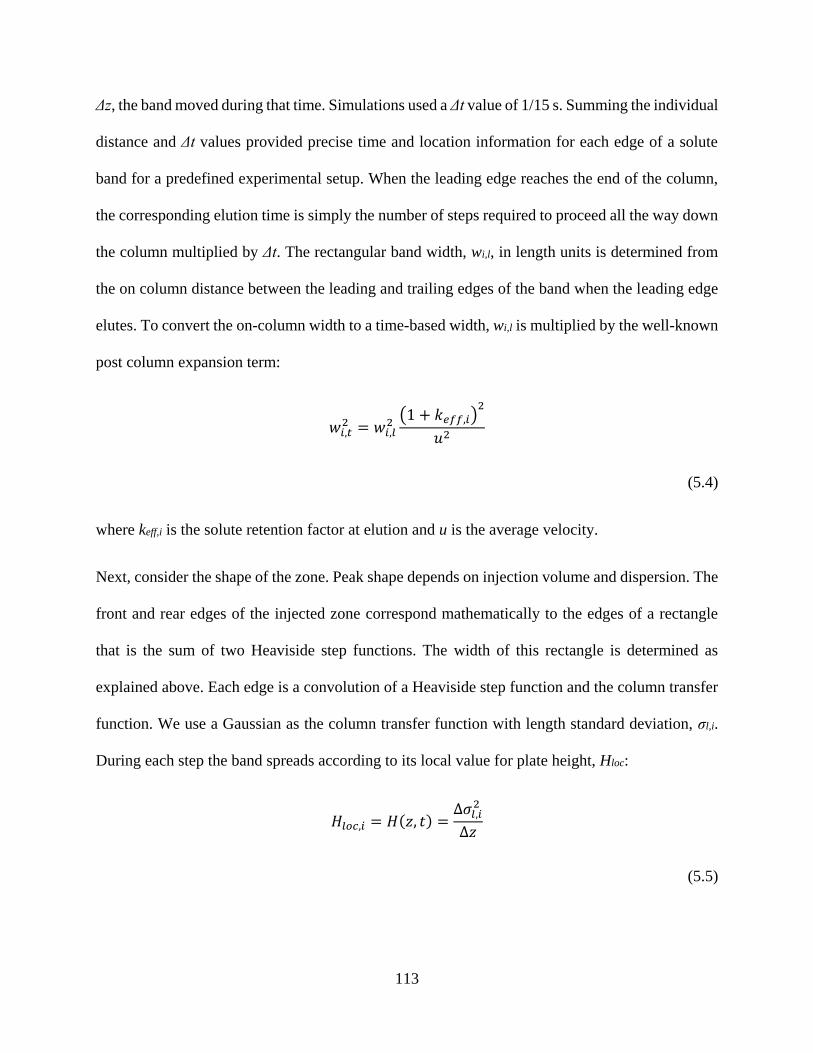
113

Δz, the band moved during that time. Simulations used a Δt value of 1/15 s. Summing the individual

distance and Δt values provided precise time and location information for each edge of a solute

band for a predefined experimental setup. When the leading edge reaches the end of the column,

the corresponding elution time is simply the number of steps required to proceed all the way down

the column multiplied by Δt. The rectangular band width, wi,l, in length units is determined from

the on column distance between the leading and trailing edges of the band when the leading edge

elutes. To convert the on-column width to a time-based width, wi,l is multiplied by the well-known

post column expansion term:

𝑤𝑖,𝑡2 = 𝑤𝑖,𝑙

2(1 + 𝑘𝑒𝑓𝑓,𝑖)

2

𝑢2

(5.4)

where keff,i is the solute retention factor at elution and u is the average velocity.

Next, consider the shape of the zone. Peak shape depends on injection volume and dispersion. The

front and rear edges of the injected zone correspond mathematically to the edges of a rectangle

that is the sum of two Heaviside step functions. The width of this rectangle is determined as

explained above. Each edge is a convolution of a Heaviside step function and the column transfer

function. We use a Gaussian as the column transfer function with length standard deviation, σl,i.

During each step the band spreads according to its local value for plate height, Hloc:

𝐻𝑙𝑜𝑐,𝑖 = 𝐻(𝑧, 𝑡) =Δ𝜎𝑙,𝑖

2

Δ𝑧

(5.5)

114

We use φ(t,z), T(t,z), values from the solvent and temperature programs to calculate each solutes’

local diffusion coefficient, Dm,loc,I, and reduced velocity, νloc,i. Local values for diffusion coefficient

were calculated by converting previously reported diffusion coefficients, Dm,i,T’, at temperature,

T’, to the local conditions, φ(t,z), T(t,z), using the following equation:

𝐷𝑚,𝑙𝑜𝑐,𝑖(𝜙(𝑡, 𝑧), 𝑇(𝑡, 𝑧)) = 𝐷𝑚,𝑖,𝑇′

𝑇(𝑡, 𝑧)𝜂(𝑇′)

𝑇′𝜂(𝑇(𝑡, 𝑧))

(5.6)

Local values for mobile phase viscosity as a function of temperature and composition were

calculated using the correlation of Guillarme et al. [26] fit to viscosity values for acetonitrile water

mixtures from Billen et al. [88]:

𝜂(𝜙, 𝑇) = 10[−2.533+742𝑇⁄ −0.452𝜙+(235

𝑇⁄ )𝜙+1.573𝜙2−(691𝑇⁄ )𝜙2]

(5.7)

Values calculated for Dm,loc,i and νloc,i were inserted into the dimensionless reduced van Deemter

equation to determine Δσloc,i2 for each particular value of Δz:

Δ𝜎𝑙𝑜𝑐,𝑖2 = Δ𝑧𝑖𝑑𝑝 [𝐴 +

𝐵

𝜈𝑙𝑜𝑐,𝑖+ 𝐶𝜈𝑙𝑜𝑐,𝑖]

(5.8)

where dp is the particle size and A, B, and C are dimensionless reduced van Deemter coefficients

measured by Zhang et al. [89].

115

Values for Δσloc,i2 calculated along the way are summed to determine a variance due to column

processes, σl, col,i2 when the band elutes from the column. Converting length to time units results

in:

𝜎𝑡,𝑐𝑜𝑙,𝑖2 = 𝜎𝑙,𝑐𝑜𝑙,𝑖

2(1 + 𝑘𝑒𝑓𝑓,𝑖)

2

𝑢2

(5.9)

Sternberg solved the convolution integral for a rectangular pulse and Gaussian distribution [161]

for the case where there is no focusing. In the presence of focusing, the injection width in time is

not the same as the band width at the exit. Incorporation of the focusing effect yields the following

equation for the concentration profile of the observed band:

𝐶(𝑡) =𝐶0𝑤𝑖𝑛𝑗,𝑡

2𝑤𝑖,𝑡[erf

𝑤𝑖,𝑡 − (𝑡 − 𝑡𝑅,𝑖)

√2𝜎𝑡,𝑐𝑜𝑙,𝑡𝑎𝑖𝑙,𝑖

+ erf(𝑡 − 𝑡𝑅,𝑖)

√2𝜎𝑡,𝑐𝑜𝑙,𝑙𝑒𝑎𝑑,𝑖

]

(5.10)

following substitution of values from Eq. 5.4; where C0 is sample concentration, winj,t, is the

injection width in time (the same for all solutes, i), 𝜎𝑡,𝑐𝑜𝑙,𝑙𝑒𝑎𝑑,𝑖 and 𝜎𝑡,𝑐𝑜𝑙,𝑡𝑎𝑖𝑙,𝑖 are the Gaussian

standard deviations calculated from Eq. 5.9 for the leading and trailing edges of the band and tR,i

is solute retention time. Note that in Eq. 5.10 erf represents the error function.

5.3.3.2 Simulating two-stage TASF with isocratic elution

To judge the effectiveness of two-stage TASF and as an initial validation of our simulation

procedure we simulated the separation of a mixture of uracil (void marker), PB2 and PB3 under

isocratic conditions. The results from this simulation are shown in Figure 5.3. Panels A, B and C

illustrate the distance traveled at any time for the solute band under the three temperature

116

conditions: isothermal (black), single-stage TASF (blue) and two-stage TASF (red), respectively.

An overlay of the simulated chromatograms is in panel D. Column dimensions were 80 mm x 0.15

mm ID, 1.7 μm dp. Injection volume was 1500 nL, flow rate was 3 μL/min, mobile phase

composition was 0.20 (w/w) water/acetonitrile, with focusing and separation temperatures of 5

and 70 °C. Focusing times for TEC A/B in the single stage TASF and TECs A/B in the two-stage

TASF simulations were 35, 35/60 s, respectively. All other chromatographic conditions used in

the simulation are in Table D4.2.

117

Figure 5.3. A) Spatial representation of isothermal chromatogram for 1500 nL injection of mixture

of void marker, ethyl and propylparaben made in mobile phase. B) Same separation under TASF

conditions, T1 = 5 °C for 35 s. C) Two-stage TASF separation demonstrating additional band

compression with second focusing stage. D) Simulated chromatogram for isothermal (black),

single-stage (blue) and two-stage TASF (red) separations.

118

From the spatial representations we can clearly see how TASF and particularly two-stage TASF

can be used to transiently modulate solute retention in chromatographically beneficial ways. In

each spatial representation, sample is injected onto the column from t = 0 until t = 30 s (Vinj = 1.5

μL, F = 3.0 μL/min). During the 30 s sample loading time, the leading edge of each solute band

traveled down the column at a velocity dictated by its local retention factor. The width of the

injection band on-column is the source of volume overload. For the simulation the local retention

factors for PB2 and PB3 under isothermal conditions were 4.4 and 10.0 at 70 °C. The on-column

width of the PB2 and PB3 bands following injection under isothermal conditions were 2.82 and

1.38 cm. In the TASF simulation, column temperature for the first 1.0 cm of the column was set

to 5 °C, so local retention factors for PB2 and PB3 increased to 15.5 and 42.3. The increased local

retention factors at the head of the column resulted in a reduction of on-column zone width for the

injection plug to 0.92 and 0.35 cm for PB2 and PB3. While volume overload was significantly

reduced by the first TASF stage the now narrowed injection zones still were not compressed

enough to induce a Gaussian shaped peak profile at the outlet of the column (blue trace in Figure

5.3D).

Addition of the second focusing segment in two-stage TASF allowed solute loaded onto segment

one (TEC A) to be released and focused again on the second 5 °C column segment (TEC B). This

second focusing effect is clearly visible in Figure 5.3C from about 0.5 to 1.0 min as the trailing

edge of both PB2 and PB3 bands velocity increased with respect to the leading edge traveling in

the cold second segment. The second focusing stage reduced solute band width further and

increased overall peak height for PB2 and PB3 by factors of 2.6 and 2.1 relative to the single-stage

TASF separations. Decreased peak width improves the overall peak capacity and resolution of the

119

separation while increased peak height benefits analysis sensitivity and quantitation figures of

merit.

5.3.3.3 Simulating two-stage TASF using solvent gradient elution

Now we extend the scope of our simulation procedure to the more complicated system of solvent

gradient elution. Figure 5.4 shows the simulation for the separation of, in order or elution, uracil

(void), HP2, PB1, HP3, PB2, HP4, PB3 and PB4 under isothermal, TASF and two-stage TASF

conditions. Darker tones in the spatial representations correspond to the paraben homologs, while

the lighter fill colors represent the hydroxyphenones. Column dimensions were identical to the

isocratic simulations. Injection volume was 3000 nL, flow rate was 3 μL/min, focusing and

separation temperatures were again 5 and 70 °C. The solvent program was a sixteen-minute linear

gradient of water/acetonitrile from 5-45% acetonitrile. Samples were made in 5% acetonitrile;

dwell time was 15 s. The focusing time for the TASF separation was 65 s, with the two-stage

separation using 65 and 100 s focusing times for TEC A and TEC B. All other chromatographic

conditions used in the simulation are in Table D4.3.

Figure 5.4A shows the spatial representation for the isothermal separation. Note that even when

using solvent gradient elution with its gradient compression effect the large sample volume and

relatively low retention factors for the early eluters still generated significant volume overload for

the separation. For clarity, retention factors for each solute under the initial gradient conditions,

k1, and at the time of elution, keff, are provided in Table 5.3. Volume overload is clearly visible for

HP2, PB1, HP3, PB3 and HP4 bands as each has a significant width at elution.

120

Table 5.3. Predicted gradient elution retention factors for each solute under isothermal and two-

stage TASF conditions.

k1, φ = 0.05 keff, 70 °C

Solute 70 °C 5 °C Isothermal

Two-Stage

TASF

p-Hydroxyacetophenone 7.2 32.7 5.3 4.0

p-Hydroxypropiophenone 24.1 135 8.0 7.3

p-Hydroxybutyrophenone 77.4 545 9.4 9.0

Methylparaben 18.5 106 7.7 6.7

Ethylparaben 63.9 454 9.1 8.7

Propylparaben 240 2290 9.9 9.7

Butylparaben 910 12000 10.3 10.3

121

As the most chromatographically interesting section of the representation is located in the first 2.0

cm of the column and initial few minutes of the simulation just the portion within the red square

(4 minutes, 2.5 cm) of Figure 5.4A are plotted for the isothermal, TASF and two-stage TASF in

panels B, C and D of Figure 5.4. Figure 5.4C clearly shows how the addition of the 5 °C focusing

segment benefited the separation by increasing k1 for all solutes. While still not compressing the

HP2 band width enough to create a Gaussian peak, width at the outlet of the column was reduced

significantly, now 0.90 cm compared to 3.70 cm under isothermal conditions. Figure 4D highlights

the importance of the second focusing segment where the 100 s TEC B focusing time was long

enough to allow the leading edge of the HP2 and PB1 bands to enter this segment, get refocused

and be released as a now narrower band. Both the HP2 and PB1 bands are focused twice. Addition

of TEC B reduced band width at the outlet of the column to 0.22 cm for HP2. Note that two-stage

TASF is a somewhat targeted technique as only solute bands moving fast enough to enter the

second cold zone prior to TEC B’s heating get focused twice. Low velocity bands, like PB3 and

PB4 do not encounter the second focusing zone at all. Fortunately, these slow-moving bands focus

well enough on their own, due to large k1 values, and do not need two-stage TASF to produce

acceptable results. This is described in more detail in the discussion of experiments below.

Figure 5.4E shows an overlay for the simulated chromatograms under the three temperature

conditions. TASF (blue) and specifically two-stage TASF (red) work to improve peak shape,

height and overall separation performance for low retention solutes. Using TASF the initial

retention factor for HP2 and PB1 were transiently increased from 7.2 and 18.5 at 70 °C to 32.7 and

106 at 5 °C. These relatively small changes and the spatial temperature program introduced using

two-stage TASF increased peak height by factors of 19.9 for HP2 and 10.7 for PB1 relative to the

isothermal control.

122

Figure 5.4. Simulations for gradient elution separations of parabens and hydroxyphenones. A)

Spatial representation for complete isothermal gradient elution chromatogram. The void maker is

bounded by dashed black lines, hydroxyphenones show as light gray bands, parabens as dark gray

bands. B) Region of isothermal spatial representation indicated by red box in panel A highlighting

segments of column subjected to temperature changes. C) Single-stage TASF spatial

representation for the first 4 minutes of the separation. Focusing time was 65 s. Light blue bands

correspond to the alkylphenones, dark blue the parabens. Band width was reduced by additional

temperature induced focusing at the head of the column. D) Two-stage TASF, alkylphenones are

shown as light red bands, parabens in dark red. p-hydroxyacetophenone and methylparaben peaks

were clearly focused twice using two-stage TASF. E) Simulated chromatograms for isothermal

(black), TASF (blue), and two-stage TASF with 100 s tfocus,B time (red).

123

5.3.4 Two-stage TASF experiments: Isocratic elution

A series of 1500 nL injections of PB2 and PB3 was made under isothermal, TASF, and two-stage

TASF conditions. Sample volume corresponded to 200% of the column fluid volume; sample

composition was fixed such that its composition matched the elution strength of the mobile phase.

Thus, any improvement in peak shape, height, or width were due to only single- or two-stage

TASF. Focusing and separation temperatures for TECs A and B were 5 and 70 °C, respectively.

TEC C and the resistively heated section of the column temperature were maintained at 70 °C.

TEC A focusing time was 35 s. TEC B focusing times were varied from 35 to 80 s in 5 s steps (up

to 70 s).

Panel A of Figure 5.5 shows the signals obtained from the isocratic two-stage TASF runs with the

nine different TEC B focusing times. What is clearly visible from the overlay is peak height

increased for both PB2 and PB3 as TEC B focusing time was increased up to a maximum (55 s,

black trace) when peak height began to decrease for PB2. Panels B and C highlight these transitions

by plotting the sections of chromatogram corresponding to PB2 and PB3. The primary objective

for two-stage TASF was to maximize concentration sensitivity, thus the optimum experimental

conditions yielded maximum detector response. Close examination of the 55 s TEC B focusing

time (black trace) chromatogram in panels B and C show the optimum focusing time for PB2 did

not correspond to the optimum focusing time for PB3. The optimal focusing time for PB2 did not

provide enough time for the PB3 band to enter TEC B prior to heating. The optimum focusing time

for PB3 was 70 s (purple trace), a value unacceptable for an analysis including PB2 as portions of

the band began exiting the TEC B before its temperature rise negating the benefits of TASF.

Differences in optimum TEC B focusing time for PB2 and PB3 were due to their difference in

retention and elution velocity.

124

Figure 5.5. A) Example chromatograms from isocratic two-stage TASF study on the optimal TEC

B focusing time. TEC A focusing time was fixed at 35 s, TEC B focusing time was systematically

increased from 35 s (corresponding to single-stage TASF) to 80 s in 5 s increments. B) Peak

profiles for PB2. C) Peak profiles for PB3. See Section 5.2.3.2.2 for chromatographic conditions.

Optimal focusing time for TEC B represented a compromise between the peak shape for PB2 and

PB3. In this example maximum peak height was desired for both solutes so a small sacrifice in

absolute sensitivity for each was made. Optimal focusing time for the conditions evaluated was

determined to be 60 s. For reference this forcing time is shown in red for each chromatogram in

Figure 5.5.

125

Figure 5.6 shows example chromatograms for isothermal (black), TASF (blue), and two-stage

TASF (red) using the optimal TEC B focusing time for the separation of uracil, PB2, and PB3.

Chromatographic conditions were identical to those used in the optimization study. Not

surprisingly single-stage TASF increased peak height for PB2 and PB3 by factors of 3.4 and 4.3,

relative to isothermal conditions. Note that single-stage TASF also decreased peak width by factors

of 3.6 and 4.6. For symmetrical peaks it is expected improvements in peak height be followed by

equivalent reductions in peak width. The marginally larger relative improvement in width for

TASF peaks was indicative of the potential for TASF to reduce peak tailing and improve peak

symmetry. A similar effect was observed in our previous work using single-stage TASF with small

volume injections where TASF was shown to significantly reduce tailing relative to isothermal

analyses [97]. PB2 peak height was increased by a further factor of 2.3 using two-stage TASF and

peak width decreased by an additional factor of 2.4 relative to single-stage TASF separation.

Improvements for the PB3 peak using two-stage TASF were similar to those for PB2, peak height

increased by a factor of 2.0, peak width decreased by a factor of 2.2. Clearly, when used

appropriately a second TASF stage can induce a multiplicative focusing effect compared to single-

stage TASF for large volume injections.

126

Figure 5.6. Overlay of isocratic chromatograms resulting from 1500 nL injections of uracil, PB2,

and PB3 samples under optimal two-stage conditions. Sample composition was made to match the

mobile phase composition. Isothermal (black) separations were performed at 70 °C. Single-stage

TASF (blue) separations had a focusing time for TEC A and TEC B = 35 s. Two-stage TASF (red)

utilized a focusing time for TEC A of 35 s, focusing time for TEC B was 60 s. Focusing and

separation temperatures for both TASF modes were 5 and 70 °C.

127

5.3.5 Two-stage TASF experiments: Gradient elution

To complete our initial assessment of two-stage TASF, we applied the approach to the separation

of a 3000 nL sample of three p-hydroxyphenones and four parabens using a linear solvent gradient.

The sixteen-minute gradient, initiated at 5% acetonitrile, had a final elution strength of 45%

acetonitrile. This gradient was performed with samples made in 5% acetonitrile. Separations were

conducted under isothermal, TASF, and two-stage TASF conditions. Focusing times for TEC A

and TEC B under TASF conditions were 65 s. Under two-stage TASF conditions, focusing times

were 65 and 100 s, respectively. All other chromatographic conditions were identical to those used

in the isocratic experiments.

Figure. 5.7 shows an overlay for representative baseline subtracted separations performed under

each temperature condition. Isothermal separations are in black, TASF in blue, and two-stage

TASF in red. Non-baseline subtracted chromatograms are provided in Figure D4.5. Panel 5.7A

shows chromatograms containing all seven retained solutes plus uracil. Uracil was added to make

the 1-minute wide injection plug more visible. The isothermal conditions resulted in unsatisfactory

chromatography. It was not until the PB3 peak that isothermal conditions yielded peaks similar to

those obtained when using either single or two-stage TASF. Most salient was the performance

improvement achieved with the addition of the second TASF stage. Two-stage TASF made the

early-eluting HP2 peak now the most prominent feature in the chromatogram.

Figure 5.7B shows the first few minutes of the chromatogram containing only HP2. Reducing

column temperature from 70 to 5 °C increased k1 for HP2 from 7.2 to 32.7. Quantitatively, TASF

improved peak height for HP2 by a factor of 7.1, relative to the isothermal separation. Addition of

the second stage increased peak height further, now by a factor of 22.3 compared to the isothermal

separation. Two-stage TASF also outperformed single-stage TASF by a factor of 3.1 for HP2 and

128

reduced its peak width by a factor of 3.5. Note that HP2 peak width (w1/2) for the 3000 nL injection,

equal to four-times the column fluid volume, was reduced to only 1.52 s using two-stage TASF.

Figure 5.7C focuses on the most hydrophobic solute in the test mixture, PB4. What is most

significant from this overlay is the lack of noticeable difference between the isothermal, TASF,

and two-stage TASF separations. Application of either TASF approach did not degrade separation

performance for the highly retained solutes.

129

Figure 5.7. A) Overlay of isothermal (black), TASF (blue), and two-stage TASF (red) separations

of hydroxyphenones and parabens. B) Excerpt of chromatograms focusing on HP2. Note the

significant differences between the isothermal, TASF and two-stage TASF chromatograms. C)

Section of the chromatogram containing PB4. Minimal differences between the separation modes

is observed indicating the neither TASF approach degraded separation performance.

130

To evaluate the potential improvement in overall separation performance for two-stage TASF

separations, values for peak capacity for the separations shown in Figure 5.7 were calculated under

isothermal, TASF, and two-stage TASF conditions. Peak capacity, nc, was calculated using the

formal definition derived by Grushka [162], shown in Eq. 5.11:

𝑛𝑐 = ∫1

𝑤1 2⁄ ,𝑖𝑑𝑡

𝑡𝑅,𝑙𝑎𝑠𝑡

𝑡𝑅,1

(5.11)

where tR,1 is the retention time for the first solute in the chromatogram, HP2 and tR,last is the

retention time for the last solute, PB4. For peak width, w1/2,i is the width at half height for each

peak in the chromatogram. The advantage to calculating nc in this fashion is that the calculation

does depend on a uniform peak width throughout the chromatogram. We have also adopted the

notion of sample peak capacity from Snyder and Dolan to define limits of integration. [163]. Plots

of the inverse peak width against retention time are shown in Figure 5.8. The isothermal separation

is in black, TASF in blue, and the two-stage separation is in red. The retention time values used

for each curve were from those obtained in the isothermal analysis. The single- and two-stage

TASF approaches shift early eluting peaks to slightly longer retention times making more space

for additional solutes early in the chromatogram, thus the use of retention times from the isothermal

analysis was the fairest method for comparison. Trapezoidal integration of the area under each

curve yielded peak capacity values of: 75, 146, and 185 for isothermal, TASF, and two-stage TASF

separations. Peak capacity improvements were most apparent early in the chromatogram, with

curves converging as solute hydrophobicity increased. What is interesting is that under the

experimental conditions this convergence does not occur until PB4 demonstrating that TASF

would improve peak shape for solutes up to those with hydrophobicity equivalent to PB4.

131

Figure 5.8. Peak capacity for isothermal (black), TASF (blue), and two-stage TASF (red)

separations from the example chromatograms shown in Figure 5.7.

5.3.6 Assessment of simulation procedure: Comparison to experimental results

The basis for the simulations is laid out in section 5.3.3.1. It will be helpful to explicitly state here

the input parameters required to generate simulated chromatograms. The program requires the

following input: injection volume, mobile phase and sample φ, TEC temperatures and their related

switching times, column length, diameter, porosities, particle diameter, dimensionless van

Deemter A, B, C coefficients and mobile phase flow rate. These are all easily specified or

controlled except for the van Deemter parameters which we took from the literature [89]. For

solutes, we experimentally determined the four parameters of the Neue-Kuss equation that define

solute k’ as a function of mobile phase composition and temperature, and we used estimates of

diffusion coefficients at 37 °C and the temperature-dependence of the mobile phase viscosity to

calculate diffusion coefficients at other temperatures. There are no adjustable parameters.

Table 5.4 displays the correspondence between experiment and simulation for the solutes used

under all conditions: no TASF, single-stage TASF, and two-stage TASF. The simulated and

132

experimental retention times are very consistent. From this, we gain considerable confidence in

several important aspects of this work. One is the value of the four-parameter Neue-Kuss equation

including extrapolation to temperatures lower than those used in establishing the parameters in

the equation. A second is the confirmation that the temperature control in the column is fairly

good. It would be difficult to determine the temperature inside the column directly. Even if it were

possible with a device like a thermocouple, the presence of the thermocouple itself would be a

major perturbation. Thus, the accuracy of the simulation across all of the experimental situations

is an indirect indication of the accuracy of the temperature control. In one sense, this should not

be surprising. Based on thermal mass, the power used to change a TEC’s temperature virtually all

goes into changing the TEC’s temperature, not the column’s. Finally, the third observation is that

the overall simulation of retention over different temperatures and solvent strengths is accurate.

This provides evidence of an effective simulation.

Table 5.4 also shows experimental and simulated peak half-widths. The agreement is reasonable.

Note that we used values of A, B, and C (dimensionless) from the literature which were based on

the same stationary phase chemistry and particle, but a different column diameter, 2.1 mm ID, and

chromatograph. This undoubtedly leads to some of the differences noted. The most striking

difference is for the very lowest k’ solute, HP2, in the gradient runs. We suspect that there may be

a secondary mechanism for solute focusing. Figures 5.6 and D4.5 show significant “dips” in the

baseline of TASF chromatograms which we suspect to be due to the changing acetonitrile

concentration in the mobile phase resulting from the change in temperature. This pulse of

acetonitrile transiently increases the velocity of the trailing edge, enhancing focusing (band

compression), but disperses as it passes down the column. Thus wider zones are more affected,

and lower k’ species have wider zones at injection than higher k’ species.

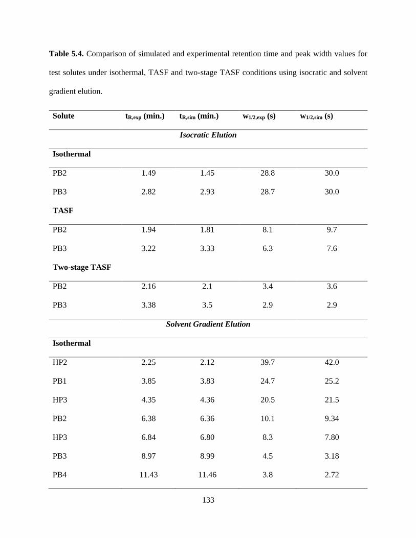
133

Table 5.4. Comparison of simulated and experimental retention time and peak width values for

test solutes under isothermal, TASF and two-stage TASF conditions using isocratic and solvent

gradient elution.

Solute tR,exp (min.) tR,sim (min.) w1/2,exp (s) w1/2,sim (s)

Isocratic Elution

Isothermal

PB2 1.49 1.45 28.8 30.0

PB3 2.82 2.93 28.7 30.0

TASF

PB2 1.94 1.81 8.1 9.7

PB3 3.22 3.33 6.3 7.6

Two-stage TASF

PB2 2.16 2.1 3.4 3.6

PB3 3.38 3.5 2.9 2.9

Solvent Gradient Elution

Isothermal

HP2 2.25 2.12 39.7 42.0

PB1 3.85 3.83 24.7 25.2

HP3 4.35 4.36 20.5 21.5

PB2 6.38 6.36 10.1 9.34

HP3 6.84 6.80 8.3 7.80

PB3 8.97 8.99 4.5 3.18

PB4 11.43 11.46 3.8 2.72

134

Table 5.4 Continued.

TASF

HP2 2.74 2.70 5.4 9.6

PB1 4.13 4.14 4.3 4.4

HP3 4.58 4.58 3.8 3.7

PB2 6.37 6.44 3.4 2.5

HP3 6.83 6.86 3.4 2.5

PB3 8.95 9.02 3.6 2.6

PB4 11.43 11.47 3.8 2.7

Two-stage TASF

HP2 3.09 2.94 1.5 2.1

PB1 4.25 4.16 2.4 2.0

HP3 4.66 4.58 3.1 3.7

PB2 6.42 6.44 3.4 2.5

HP3 6.88 6.86 3.5 2.5

PB3 8.97 9.02 3.6 2.6

PB4 11.44 11.47 3.8 2.7

135

5.3.7 Advantages and limitations

We built a device consisting of three, independently controlled variable temperature segments for

use in packed-column cLC. We used this device to improve on our previously developed TASF

concept, demonstrating the ability of the new design to focus on-column bands twice using the

two-stage TASF approach. The three-TEC system also provides more experimental flexibility than

our previous systems composed of a single one-cm long focusing segment. The three TEC system

can be operated in the single-stage TASF mode with variable length focusing dimensions, namely

one-, two- or three-cm long segments. Longer focusing segments facilitate the use of larger

injection volumes improving analysis sensitivity without observing band “leakage” from cold to

hot column zones. Leakage degrades TASF performance (see Figure 5.5). Further, the linear array-

based TEC configuration allows for dynamic temperature changes in non-TASF applications. For

example, TECs can control retention of selected solutes by controlling temperature at particular

locations along the column at particular times. We view the work presented here using two-stage

TASF as a first step towards developing the ability to module retention in a reliable and

predictable way down the entire length of the cLC column.

While the device presented is a significant advance on our previous single TEC devices, it is not

without limitations. The current configuration has discrete 1-cm long focusing zones. Systems

composed of smaller, ca. 0.5 cm, variable temperature segments offer certain experimental

advantages. The primary advantage to smaller TECs is the ability to use only the required focusing

zone length for the desired solute, injection volume and focusing temperature. Cooling portions of

the column not used for actual focusing wastes system pressure making it unavailable to the

practitioner to increase column length or analysis speed. (Pressure is directly related to viscosity

and viscosity is temperature dependent, usually increasing with reduction in temperature.) A

136

second limitation of the current design concerns TEC lifetime. TECs in our hands last for hundreds

of TASF cycles, but they do wear out eventually becoming unable to change temperature at all. In

the current configuration all three TECs are soldered to a single copper heat sink. Repair

necessitates the entire heat sink assembly must be disassembled to replace a single malfunctioning

TEC. This is the primary limitation of the current design when routine operation is desired. We

are in the process of optimizing heat sink design to solve this problem.

5.4 CONCLUSIONS

In this work we have demonstrated through accurate simulation and experiment the potential to

focus injection bands twice on-column using a process called two-stage TASF. This sequential

temperature-based focusing approach presented is not achievable using the more common solvent-

based approaches. We have validated its efficacy using simulation and shown experimentally its

ability to reduce sample-induced dispersion in isocratic and gradient elution liquid

chromatography. We can draw the following conclusions:

1. Linear arrays of closely spaced TECs can be used effectively to modulate solute

retention in a space and time dependent way.

2. The simple simulation procedure based on local retention factors accurately predicts

experimental band location and shape under isocratic and solvent gradient elution

conditions. Simulations match experiments.

3. The addition of a second TASF stage induces a multiplicative focusing effect when

used under isocratic conditions. The effect roughly doubles that observed for low

retention solutes under single-stage TASF conditions.

137

4. Solvent gradient elution also sees significant benefit from the two-stage TASF

approach, increasing peak capacity for a simple test mixture by a factor of 2.5 relative

to an isothermal control.

These results demonstrate the potential for the broader application of dynamic temperature

changes in capillary liquid chromatography to modulate solute retention in chromatographically

useful ways using simple, reliable and relatively inexpensive hardware.

138

6.0 GRAPHICAL METHOD FOR CHOOSING OPTIMIZED CONDITIONS

GIVEN AN PUMP PRESSURE AND A

PARTICLE DIAMETER IN LIQUID CHROMATOGRAPHY

The contents of this chapter were previously published in: Groskreutz, S. R. and Weber, S.

G. Analytical Chemistry, 2016, 88 (23), 11742-11749.

Reproduced with permission from the American Chemical Society.

6.1 INTRODUCTION

It takes time to get information about a sample from liquid chromatography. How much depends

on the nature of the question and the sample. It also depends upon several parameters related to

the liquid chromatographic (LC) system itself. The complexity of chromatographic instruments

and the significant number of parameters that control them has spawned many efforts to

systematize procedures for optimizing the performance of packed-bed LC which are cited below.

Graphical depictions of chromatographic performance as a function of parameters and variables

can be useful because they contain a lot of information, however the sheer number of parameters

in modern LC confounds efforts to create simple graphics in a two-dimensional format that are

easily interpreted. In this work we briefly review previously developed optimization diagrams and

present a new graphical approach to determine optimized LC parameters for practitioners wishing

to maximize isocratic plate count (N) or peak capacity in gradient elution (nc) in a given analysis

time when using a particular particle diameter and pump pressure.

139

Most famously, van Deemter et al. developed a plot that continues to guide virtually all reasoning

about chromatographic optimization [164]. The van Deemter plot arose from their application of

the mass balance approach [4, 5] to solving for a chromatographic band width as a function of

mobile phase velocity. Based on earlier work by Klinkenberg and Sjenitzer [165], van Deemter et

al. put meat on the bones of the theoretical plate concept of Martin and Synge [1]. What leaps out

of the van Deemter plot is the presence of a minimum in theoretical plate height, the change in

zone variance (in length units) with a change in zone position as it travels down the column. But,

until recently, working at a velocity corresponding to that minimum made for chromatographic

run times that were uncomfortably long. Thus, “Ultimately all questions about optimization are

related to a compromise between efficiency and time” [28]. Key parameters in realizing a

particular chromatographic figure of merit are the available pressure and the particle diameter. The

former limits the column length’s magnitude, L, and the degree to which particle diameter, dp, can

be decreased. The latter, as well as partly governing the pressure required is also a significant

parameter in the van Deemter equation which bounds separating power. These limitations and

opportunities have been described in a number of key papers, and interesting plots, in the decades

of the ‘60s – ‘80s [166-172] some of which we return to below.

Many graphical illustrations of chromatographic performance have been designed to explore the

effect of key parameters like particle diameter, pressure, and temperature. The plots that result

provide information at three limits: What is the effect of the chosen parameter on the maximum

number of theoretical plates? On the highest speed? On the position of the minimum height

equivalent to a theoretical plate, H? Giddings’s used a so-called kinetic plot to demonstrate the

limiting performance of an LC system over long and short timescales in comparison to GC (Figure

E5.1 in Appendix E) [167]. The clear conclusion from the plot was that LC will provide more

140

theoretical plates at long times, but GC will be capable of more theoretical plates with higher speed

at short times. The long time limit of the plot is equivalent to about 30 years. While the plot clearly

makes its point related to the comparison of GC and LC, it does not provide easily accessible

information for practitioners about how to achieve the best performance at reasonable times.

Similarly, Knox and Saleem [168] compared LC and GC over a wide range of conditions

specifying those required to operate at or near the minimum H while using some or all of the

available pressure. Again data are plotted (Figure E5.2) over many orders of magnitude focusing

attention at the limits of chromatographic performance. Flow rates near the maximum hypothetical

value of ν correspond approximately to filling an Olympic sized swimming pool every 30 minutes

with mobile phase passing through a 2.1 mm ID column. Clearly, the point of these early plots is

to illustrate broadly the best approach to attain a large number of theoretical plates, or achieve a

certain effective number of theoretical plates in a given time.

Poppe reinvigorated the discussion of separation power in a paper comparing various formats for

liquid-phase separations including pressure-based chromatography [173]. This work led to another

graphical approach to chromatographic optimization that came to be known as the Poppe plot

which expresses the plate time (t0/N) as a function of N (Figure E5.3). More recently, the Desmet

group demonstrated the information content in a family of kinetic plots [174-183] (Figure E5.4)

developed to expand on the separation impedance concept developed by Knox [184]. These plots

speak more directly to practical figures of merit over a very wide range of conditions for different

chromatographic supports. The Carr group expanded on that of Poppe to generate a plot for

gradient peak capacity production [185]. The same group also clarified the algebraic relationships

among the interacting parameters in liquid chromatography [28]. The latter work is quite helpful

as it clearly distinguishes two important cases: global optimum (maximum plates per time given a

141

certain pressure and mobile phase viscosity) which they called the three-parameter problem, and

the two-parameter optimization when one additional parameter, usually dp, is fixed. Although not

as crisply articulated, it is noteworthy that Knox and Saleem described the same thing in 1969

[168]. There is no question that plots have great value for understanding in broad strokes how to

think about chromatographic optimization.

Both Guiochon [172] and Halasz and Görlitz [186] created nomograms for estimating laboratory

conditions (Figures E5.5 and E5.6). While they do cover a rather wide range of conditions they

are also useful for determining actual experimental conditions. For example, in Figure E5.5, we

illustrate how to find conditions to do a one-minute separation (k’ = 3, mobile phase viscosity = 4

x 10-4 Pa s) with 600 bar pressure: the particle size should be 1 μm. Similarly, the Halasz and

Görlitz plot can be used to deduce similar information. For a k’ = 3 and a one-minute separation,

t0 is 15 s. The intersection of that value and P = 600 bar is shown approximately as a dot on Figure

E5.6. This guides us to a particle size of about 1.5 μm. Chen and Horvath arrived at similar

conclusions for separations of small and large molecules using reasoning analogous to that of

Guiochon [187]. Later Meyer extended the Halasz and Görlitz nomogram concept to maximize

isocratic and gradient peak capacity [188, 189].

In the process of working on fast neurotransmitter separations, we have realized a need for a plot

that illustrates these same concepts, but that also fulfills three other criteria: (1) it is accessible to

a non-expert, (2) it is focused on practical parameter ranges over a few powers of 2, not several

orders of magnitude, reflecting reality in the lab, and (3) provides experimental parameters of

column length and velocity immediately. Here, we explain the plot and demonstrate its value in

determining conditions to achieve certain objectives from applications taken from our laboratory

under isocratic and gradient elution conditions.

142

6.2 THEORY

6.2.1. Information needed to construct the plot

Estimates, of the plate height/velocity and pressure/velocity relationships are required to construct

optimization graphics. Thus, step one involves selection of the desired solute, mobile phase

composition and column temperature. The latter two parameters play a critical role in determining

chromatographic performance due to their influence on eluent viscosity and analyte diffusivity.

Step two comprises a flow study to measure the kinetic and permeability properties of the column.

We used 𝐴, 𝐵, and 𝐶 values in the reduced van Deemter equation shown in Eq. 6.1 from Zhang

et al. [89] for columns packed with 1.7 μm fully porous particles. Conditions used in the calculation

were 25 °C, with a 96:4 water/acetonitrile mobile phase. (Other chromatographic conditions are

provided below.)

ℎ =𝐻

𝑑𝑝= 𝐴 +

𝐵𝐷𝑚

𝑢𝑒𝑑𝑝+

𝐶𝑢𝑒𝑑𝑝

𝐷𝑚

(6.1)

where ℎ is the reduced plate height, 𝐻 is the dimensioned plate height, 𝑑𝑝 is the particle size, 𝐷𝑚

is the solute diffusion coefficient in the mobile phase, 𝑢𝑒 is the interstitial linear velocity and 𝐴,

𝐵, and 𝐶 are the reduced dimensionless van Deemter coefficients.

It requires pressure to force eluent through a chromatographic column. Eq. 6.2 shows a

semiemperical equation derived from Darcy’s law which relates column parameters to pump

pressure, 𝑃, under conditions typically experienced when fluids are passed through packed beds.

143

𝑃 = 𝛷𝜂𝑢𝑒𝐿

𝑑𝑝2

(6.2)

The plots require the dimensionless flow resistance parameter, 𝛷, from Eq. 6.2 which can be

determined from the slope of pressure vs velocity data. Here, we have used 𝛷 and column porosity

values, εe and εtot, reported by Zhang et al.[89] in our calculations.

Numerical values used in subsequent optimization calculations are provided in Table 6.1.

144

Table 6.1. Parameters used in optimization plots.

Parameter Source Value

Pmax (bar) Instrument 600, 1000

Dm,25 °C (cm2/s) Literature [190] 5.6×10-6

Dm(φ,T) Literature [99] See Eq. E5.1

A Literature [89] 0.66

B 10.2

C 0.095

dp (μm) 1.7

Φ 431

εe 0.353

εtot 0.537

Tcol (°C) Experience 25

φ 0.04

η(φ,T) (cP) Literature [26, 88] See Eq. E5.2

145


6.3.1. Introduction to the plot

Figure 6.1 shows an example of a plot generated from the values in Table 6.1 and equations 6.1,

6.2, and the well-known relationships among average velocity, interstitial velocity and porosity,

and among average velocity, length, and time. The vertical axis represents column length (cm);

the horizontal axis interstitial velocity, ue, (cm/s). Dashed lines indicate constant values for t0, from

1 to 80 s with particular values indicated adjacent to each line. Colored contour lines denote

constant values of N. Contours begin with N = 1000 and increase in 1000 plate divisions until N

= 10000, where spacing increases to 5000 plates per division up to a maximum of 30000 plates.

At any point on the plot, a value of ue can be chosen which (with data from Table 6.1) provides a

plate height. Then a value of L can be chosen which provides a value of N. The values of ue and L

immediately dictate t0. For example, near the top of the plot, we see that 20000 theoretical plates

can be generated (purple line) with a t0 of 20 s by using approximately a 15 cm long column and

a ue of 1.0 cm/s. Of course, not all lengths and velocities are accessible because the available

pumping pressure is a limitation. Black hyperbolas are constant pressure isobars for 600 and 1000

bar. Conditions below and to the left of these hyperbolas are achievable combinations of L and ue

for systems with 600 and 1000 bar limits. Thus, we see that the 20000 theoretical plate/20 s t0 point

is not accessible even with a 1000 bar system (at 25 °C). Optimum conditions occur along an

isobar. While one can operate below the isobar, performance is better when the operating point is

on the isobar. Values of L, ue, t0, and N along the isobar are referred to by Carr et al.[28] with

asterisks, e.g., L* etc. To summarize, for a given dp and T (and other particular attributes of the

system as in Table 6.1), each point on this plot represents values of L, ue, t0, and N. One cannot

operate to the right of an isobar. Operating to the left is permissible. Operating on the isobar is

146

best. Points along any isobar correspond to the results of Carr at al.’s “two-parameter” optimization

[28] for a given Pmax.

Figure 6.1 presents a significant amount of useful information regarding optimization concepts

and chromatographic performance. First, ignore for the time being the need for a particular

pressure and focus on the contour lines for N. The constant plate contour lines reflect the shape of

the van Deemter curve. This can be understood by following a horizontal, constant L, trajectory

across the plot. Consider L = 9 cm. For the lowest interstitial velocity, N is low. As velocity

increases, N increases over 10000 then reaches a maximum of about 20000 where the contour line

reaches a minimum near ue = 0.33 cm/s and t0 about 40 s. The minimum in the contour line for N

represents the shortest column at which that number of theoretical plates can be generated. As

velocity is increased further, N decreases. This is consistent with the fact that N = L/H (Eq. 6.1

and L is constant). As a vertical trajectory is taken at constant velocity, N increases steadily, again

in agreement with N = L/H (and H is constant). The B-term region of the van Deemter curve

corresponds to the left side of Figure 6.1 where linear velocity is below the optimum of 0.33 cm/s.

This is the long L, long t0 section of the plot. The C-term dominated portion of Figure 6.1 is in the

lower right corner and corresponds to short columns and analysis times.

Now, let us consider the case where we will use the maximum pressure of 600 bar. Under what

conditions can we obtain 20000 theoretical plates as we did for L = 9 cm, ue = 0.33 cm/s, t0 ~ 40 s

at the van Deemter optimum velocity? The 20000 theoretical plate contour crosses the 600 isobar

at the point designated by the letter A. Operating at 600 bar maintains the plate count but decreases

t0 to about 35 s.

147

Figure 6.1. Plate count, t0, and P as a function of ue and L (given the parameters in Table 6.1). A)

Conditions required to generate N = 20000 in the shortest time, t0 = 35 s, for a pump with a 600

bar pressure limit. B) Conditions that represent the maximum N for t0 = 63.7 s for the 600 bar

system. This point is often referred to as the Knox-Saleem limit where velocity is set to the van

Deemter optimum and column length sufficient to operate the system at its pressure maximum. C)

Points required to generate 2000 plates for the 600 and 1000 bar systems where the increase in

system pressure has little influence on chromatographic speed.

148

There is one place where the isobar crosses a constant N curve at its minimum indicated by the

letter B: It is at the van Deemter optimum velocity with column length such that system pressure

equals Pmax. The conditions for point B are: Pmax = 600 bar, ue = 0.33 cm/s, L = 13.4 cm, t0 = 63.7

s and N = 30000. Conditions represent the maximum N for t0 = 63.7 s for the 600 bar system with

1.7 μm particles at 25 °C. This is the only point on the isobar that is at the van Deemter optimum

velocity. This point is frequently referred to as the Knox-Saleem limit [28, 29, 191].

Supposing we desire a t0 of 20 s with a 600 bar system pressure limit? From the plot, we can expect

that 15000 theoretical plates are generated using a 7.5 cm long column at a linear velocity of 0.57

cm/s. The plot is also useful for a rapid assessment of the consequences of using a particular

column length, e.g., 5, 10, or 15 cm.

Further, the plot helps to see whether increasing pressure can aid the chromatographer who is

interested in speed, for example, t0 < 5 s. A system with a 600 bar limit generates 2000 plates for

a t0 = 1.8 s (Figure 6.1 points C). Increasing Pmax to 1000 bar has a negligible impact on speed for

the 2000 plate separation, decreasing t0 only 0.1 s. Clearly increasing system pressure alone is not

a viable solution to increase speed under these conditions. Graphically, this information is evident

as follows: constant t0 lines are practically parallel to the constant plate contours. Traveling along

a constant t0 line is achieved by changing pressure while changing L and ue proportionally. On the

other hand, if system pressure is increased with a commensurate decrease in particle size both plate

count and separation speed are improved [28]. It is fair to say that, while this plot tells the reader

that increasing pressure alone when working on high-speed separations will have minimal effect

on separation quality, it does not explain why. Probably the algebraic representation as expressed

in Carr et al. [28] (particularly the discussion centered around eqs. 14 – 17) is the best way to

understand why this is the case.

149

6.3.2 Application of the plot to several problems

With this orientation to the plot, we now demonstrate the efficacy of Figure 6.1 based on our

laboratory’s applications. We have an interest in neurochemistry, specifically the study of

monoamine neurotransmitters serotonin (5-HT) and dopamine (DA) in vivo by microdialysis

coupled online to LC. Changes in 5-HT and DA concentration are measured in response to various

chemical and physical stimuli in vivo using online LC. The speed of the separation currently limits

the time resolution. Better time resolution means we can extract more information.

In our first demonstration of the graphic in Figure 6.1 we require the quantitative determination of

5-HT by LC coupled online to microdialysis with high time resolution. Thus, high speed conditions

are required, while the separation must also generate a predetermined number of plates to ensure

accurate quantitation. This is a classic two-parameter optimization problem. Temperature, particle

diameter, and pressure are the major elements of chromatographic optimization. Thus, we use the

plot to assess the role of elevated column temperature and different particle sizes to improve the

speed of our neurotransmitter analyses. Our application yields small sample volumes (10 – 500

nL) with low concentrations, thus quantitation is a challenge. Selection of the best column diameter

represents a compromise between sample dilution (diameter too large) and volume overload

(diameter too small). In a second demonstration we have incorporated the influence of volume

overload into the neurotransmitter optimization procedure. Finally, we expand the scope of the

plot from purely isocratic elution using the theoretical plate concept to gradient elution to increase

the peak capacity production for the analysis of neuropeptide mixtures.

150

6.3.3 Maximizing isocratic plate count for fixed analysis time

For accurate quantitation neurotransmitter separations require a few thousand theoretical plates –

here we specify 5000 theoretical plates. We focus on 5-HT, results are similar for DA.

Chromatography uses “ion-pairing” reversed phase LC, with a small portion of acetonitrile in the

mobile phase, 96:4 aqueous/acetonitrile, to achieve k’ ~ 10 [99]. In Figure 6.2A, the red point is

at 5000 theoretical plates and 600 bar. It has been calculated for 5-HT using 1.7 μm fully porous

particles and a column temperature of 25 °C (see Table 6.1 for conditions). Under the 5000 plate

requirement we see from the light yellow contour, 5000 plates are generated with a t0 of about 5 s

for the 600 bar limit system. 5-HT retention time is 55 s and time resolution is one minute. These

results are similar to our previous in vivo work with 1-minute temporal resolution separations of

5-HT and DA [92, 192]. Now the question becomes how can we adjust chromatographic

parameters to achieve the necessary 5000 plates in less time to improve temporal resolution.

Briefly, we again consider what benefit there is to increasing pressure alone as shown by the blue

arrows. Blue arrows illustrate the effects. The column’s length could be increased to provide more

plates, but the chromatographic time increases. The velocity could be increased, decreasing t0

significantly, but with a concomitant decrease in plates. One could adjust length and velocity to

keep N constant, but only a very small increase in speed would be gained. While it cannot be stated

that increasing pressure does not help for a t0 = 5 s separation, it helps very little to increase speed

without sacrificing efficiency. Fortunately, there is a simple solution to help increase speed.

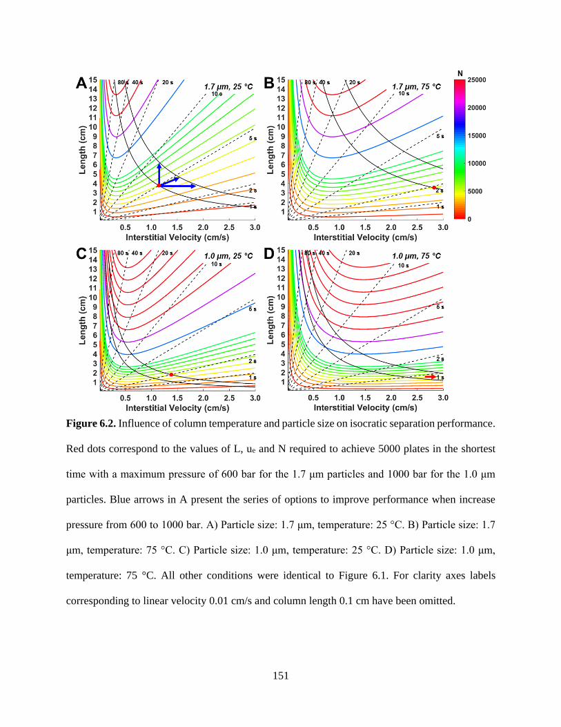
151

Figure 6.2. Influence of column temperature and particle size on isocratic separation performance.

Red dots correspond to the values of L, ue and N required to achieve 5000 plates in the shortest

time with a maximum pressure of 600 bar for the 1.7 μm particles and 1000 bar for the 1.0 μm

particles. Blue arrows in A present the series of options to improve performance when increase

pressure from 600 to 1000 bar. A) Particle size: 1.7 μm, temperature: 25 °C. B) Particle size: 1.7

μm, temperature: 75 °C. C) Particle size: 1.0 μm, temperature: 25 °C. D) Particle size: 1.0 μm,

temperature: 75 °C. All other conditions were identical to Figure 6.1. For clarity axes labels

corresponding to linear velocity 0.01 cm/s and column length 0.1 cm have been omitted.

152

When column temperature is increased the mobile phase viscosity decreases significantly, e.g., η75

°C = 0.4 cP, η25 °C = 0.9 cP. This viscosity decrease has the same mechanical effect as increasing

the system pressure limit: for the same packed bed, the mobile phase velocity and thus separation

time (all else constant) are improved resulting in an increase in speed. At the same time, there is

an increase in 5-HT diffusion coefficient, Dm,75 °C = 1.4×10-5 cm2/s, Dm,25 °C = 0.54×10-5 cm2/s,

which is an increase of a factor of 2.6. In high-speed separations where the van Deemter C-term is

important we note that the C-term is proportional to the parameter 2 /p md D . Increasing temperature

has an effect that is similar to decreasing particle diameter.

Let us return to the 5-HT problem. Increasing the column temperature to 75 °C while maintaining

N ≈ 5000 should increase speed. As Figure 6.2A and B show, this is indeed the case. Now, for

Pmax = 600 bar, N = 5000 is achieved with t0 = 1.9 s, L = 3.5 cm, ue = 2.81 cm/s (red point, Figure

6.2B). This corresponds to a retention time of 21 s for 5-HT and an analysis time of 25 s. Increasing

column temperature would permit 30 s time resolution in the microdialysis experiment. It is

interesting to compare the effect of decreasing particle diameter, Figure 6.2C shows the same plot

as Figure 6.2A with dp = 1.0 μm, T = 25 °C. The line for 5000 plates and 600 bar cross at about L

= 1.5 cm and ue = 1.0 cm/s with t0 = 2.3 s. The decrease in particle size has a similar effect on the

separation quality as raising the temperature, although the speed is 20% poorer. Increasing the

available pressure to 1000 bar (red dot, Fig. 6.2C) provides virtually equivalent performance to

the 75 °C, 600 bar, 1.7 μm particle, case (Fig. 6.2B). Finally, we can see from the red arrow in

Figure 6.2D that increasing the temperature from the conditions in Figure 6.2C more than halves

t0 to an impressive 0.8 s with L = 1.7 cm, ue = 3.4 cm/s and N = 5000 (location of point not shown).

153

Finally, and briefly, we have been discussing the creation of non-standard length columns. This is

not a problem for capillary columns packed in-house, but these plots readily provide useful

information about the performance of columns of fixed length at various conditions.

6.3.4 Volume overload and its impact on optimization

Basal 5-HT concentration in vivo in the rat striatum is about 1 nM or less, sample volume is 500-

1000 nL, consequently accurate quantitation for online neurotransmitter monitoring requires

detection limits sufficient to determine quantitatively ~ 1 fmol or less. It is important to minimize

the volume of the chromatographic zone that contains that femtomole to achieve the highest

possible signal from a concentration sensitive detector. Thus, to avoid significant dilution,

capillary columns are used. Column volume is typically 200-500 nL. Under these conditions

injection volume often is equivalent to, or may exceed the column fluid or dead volume. Large

volume injections can result in a phenomenon known as volume overload. Volume overload occurs

when the injection volume contributes significantly to the observed band spreading, decreasing the

apparent efficiency of the separation. It is worth noting that this phenomenon was explored by van

Deemter et al. in their seminal 1956 paper [164].

The combination of on-column- and volume overload-induced band spreading leads to an observed

column efficiency, Na, shown in Eq. 6.3:

𝑁𝑎 =𝐿

𝐻𝑎=

𝐿

𝐻 + (𝜎𝑖𝑛𝑗

2

𝐿⁄ )

(6.3)

154

where L is column length, Ha is the apparent plate height, H is the non-overload plate height

(calculated as above), and 𝜎𝑖𝑛𝑗2 is the injection variance. The injection variance is a function of the

injection volume, column volume and solute retention factor in the sample solvent [193]. Figure

6.3 shows the plot with contours of Na, rather than the column’s intrinsic plate count, N. The

apparent plate count has been calculated for fixed 125 nL injections into 100 (A), 150 (B) and 250

(C) μm ID columns while the remaining parameters are as in Figure 6.2B. Holding the injection

volume constant reflects the situation in online analysis (e.g., microdialysis) in which the fixed

time resolution corresponds to a particular, fixed volume of sample from a constant flow rate

stream. The solute retention factor in the sample solvent was 10. What is most obvious from Figure

6.3A is the significant loss in observed column efficiency due to the 125 nL injection. Under the

same conditions optimized for speed in Figure 6.2B, indicated by the red dot, N = 5000, t0 = 1.9 s,

L = 3.5 cm, ue = 2.81 cm/s, plate count has decreased from 5000 to 1430.

It is also noteworthy to see the reflection of Eq. 6.3 in Figure 6.3A. The injection variance term is

not velocity dependent. As a result, for short columns where the injection variance term is largest

for a fixed injection volume and column diameter the Na contours are flat at sufficiently high

velocities.

Apparent column efficiency when injecting 125 nL onto the 100 μm ID column does not yield the

required 5000 plates for accurate quantitation. There are several solutions available to regain

column efficiency: decrease injection volume, increase column length, increase column diameter,

improve focusing. Reducing injection volume increases efficiency by reducing volume overload

effects, but a smaller volume injection decreases detector signal as the 5-HT average concentration

in the eluting peak will have decreased. This is not a desirable solution. Increasing column length

adds plates, improving the separation, but also adds time to the separation. The purple dot in Figure

155

6.3A shows this, for Na = 5000, L = 6.9 cm and t0 = 7.2 s. Improving sample focusing (increase k’

in the sample solvent) is the best solution to maintain efficiency with large injection volumes, but

is not always simple to implement. Thus we focus on the role of column diameter. Previously we

have shown this parameter to be critical to the optimization for speed and sensitivity [99]. Figure

6.3B and 6.3C highlight this importance. As in Figure 6.3A purple dots in 6.3B and 6.3C show the

conditions required to achieve Na = 5000 in the shortest time (operating at Pmax = 600 bar). Open

dashed circles in each panel represent the conditions for the target 1.9 s t0 and 30 s temporal

resolution microdialysis experiments. For the 150 μm ID column in Figure 6.3B 5000 plates are

generated using L = 4.4 cm, t0 = 3.0 s and ue = 2.24 s. Increasing diameter to 250 μm results in

conditions in which L = 3.6 cm, t0 = 2.0 s and ue = 2.75 cm/s, virtually identical to the parameters

found without volume overload.

156

Figure 6.3. Effect of volume overload and column diameter on apparent column efficiency

optimization for 1.7 μm diameter particles. A) 100 μm ID column, B) 150 μm ID column, C) 250

μm ID column. The red dot in panel A corresponds to the values of L, ue, and N required to generate

5000 plates in the shortest time for a 600 bar pressure maximum shown in Figure 6.2B. Open red

circles in B and C represent the target conditions indicated by the red dot in A. Purple dots in each

panel denote the new conditions required to achieve 5000 plates factoring in volume overload

effects. Injection volume was 125 nL, retention factor in the sample solvent was 10, column

temperature was 75 °C. All other conditions were identical to Figure 6.1. For clarity axes labels

corresponding to linear velocity 0.01 cm/s and column length 0.1 cm have been omitted.

157

6.3.5 Peak capacity optimization in gradient elution separations

Thus far we have optimized performance of isocratic separations using a series of graphics based

on Figure 6.1. Under gradient conditions, peak capacity is the most relevant metric to assess the

performance of a separation [7]. In this section we have reformatted Figure 6.1 to optimize

separations of neuropeptides by maximizing peak capacity at a given gradient time. Neuropeptides

are an important class of signaling molecules in the brain, regulating processes involved with pain

and learning [194]. We have a longstanding interest in the fate of neuropeptides in the brain,

specifically their hydrolysis by ectopeptidases [195, 196]. To understand the kinetics of

neuropeptide hydrolysis, samples must be analyzed using solvent gradient elution to efficiently

separate moderately hydrophobic peptides from their often very hydrophilic hydrolysis products.

We illustrate this with an example, the quantitative analysis of leucine enkephalin (YGGFL) and

its primary hydrolysis product in tissue, GGFL. Inclusion of sampling and LC internal standards

yields a relatively simple mixture composed of four solutes accessible with isocratic elution [196].

However, much more biochemical information could be obtained by simultaneously determining

other products such as YG, YGG, GFL, and FL. Gradient elution would be the best approach.

Furthermore, other neuropeptides and their products span an even greater range of hydrophobicity

which requires a gradient method for analysis.

Using an approach similar to that for creating Figure 6.1 we calculated values for peak capacity,

nc, using Neue’s formulation [7]:

𝑛𝑐 = 1 +1

4𝑁(𝑡𝑜, 𝐿, 𝑢𝑒)

12⁄

1

𝐺 + 1ln [

𝐺 + 1

𝐺𝑒𝑆∆𝜑 −

1

𝐺]

(6.4)

158

were N is the column efficiency, a function of t0, L, and ue, S is the slope of the log of solute

retention factor vs eluent composition from Snyder’s linear solvent strength theory [193], Δφ is

the range in eluent composition and G = SΔφt0/tG, tG is the gradient time.

Figures 6.4A and 6.4B show peak capacity optimization plots similar to Figure 6.1 for the analysis

of leucine enkephalin hydrolysis mixtures using short linear gradients. Axes remain L and ue,

dashed lines indicate constant t0, solid black lines show 600 and 1000 bar system limits. Colored

contour lines in Figure 6.4 represent constant values of nc calculated from Eq. 6.4. Contour spacing

in Figures 6.4A and 6.4B are 12.5 peak capacity units. Conditions were: S = 20 (lower limit for

small peptides) [197], Δφ = 0.5, tG = 1 and 3 minutes, dp = 1.7 μm, T = 25 °C. For simplicity van

Deemter coefficients matched those in Table 6.1 and plate height dependence on mobile phase

composition was neglected. Column efficiency and pressure were calculated with mobile phase

composition set to 0.2 acetonitrile/water. The diffusion coefficient for leucine enkephalin in water

is Dm,25 °C = 4.1×10-6 cm2/s [190]. The diffusion coefficient for leucine enkephalin under specific

conditions of mobile phase composition and temperature was calculated using Eqs. E6.1 and E6.2.

What is obvious from Figures 6.4A and 6.4B is the difference in shape for the constant peak

capacity contours for each gradient time and presence of a clear nc maximum which is seemingly

independent of column dimensions and system pressure. Unlike the isocratic efficiency plots

(Figure 6.2) where characteristic van Deemter-curve shapes are visible under all conditions the

peak capacity analogs provide a less consistent general shape, but one which is highly dependent

on gradient time. At short gradient times it is particularly obvious that the contours have a shape

that is different from the contours of N in the isocratic case. In both the isocratic and gradient plots,

for a given length, there is an optimum velocity (reminder: irrespective of pressure limitations).

However, only in the gradient plots is there also an optimum length for a given velocity.

159

Figure 6.4. Plots for gradient elution peak capacity as a function of ue, L and tG for separations of

neuropeptides. Gradient times were: A) 1 minute, B) 3 minutes, C) 20 minutes, D) 60 minutes.

Particle size and column temperature were 1.7 μm and 25 °C, respectively. See text and Table 6.1

for other chromatographic conditions. For clarity, axis labels corresponding to linear velocity 0.01

cm/s and column length 0.1 cm have been omitted.

160

Now we return to the enkephalin separation. In Figure 6.4A, with 1000 bar pressure, the maximum

value of nc is 81 (purple dot). However, the contour becomes quite flat in this range of lengths and

velocities for short tG (See Figure E5.8). Thus, lengths from about 3 – 6 cm with appropriate

adjustments in velocity yield nc greater than 75 for the one-minute gradient. Operating at a pressure

of 600 bar, where the maximum value of nc is 80 (red dot), involves no practical sacrifice. As with

the isocratic separations, in this regime of speed there is little to be gained from increasing pressure

alone.

If we relax the time requirement, Figure 6.4B shows similar general properties at tG = 3 min but

with increased maximum peak capacity: 133 at 1000 bar and 128 at 600 bar. When considering

the two upper graphs with reasonably brisk separations, we note that the optimum t0 hardly changes

with changes in pressure. Further, the optimum tG/t0 is in the mid-teens.

As mentioned above, we might ask the question, “If we challenge tissue with a small number of

neuropeptides, what is the best approach to separation and quantitation of all detectable

components in the mixture following hydrolysis in the tissue?”. If we were to perfuse tissue with

three neuropeptide substrates and expect 3 – 4 quantifiable products from each, the separation

would focus on 9 -12 peaks, a rather modest number. Even so, the statistical peak overlap theory

[198] tells us that for a 90% likelihood of a clean separation of 12 components we would need a

peak capacity of 228; for a 95% probability it would be 468. From Figure 6.4C we see that to

achieve a peak capacity of 228 with 1.7 μm particles at 25 °C with a 1000 bar system limit

(indicated by the red dot) we need to use a 20-minute linear gradient, a 5.9 cm column and set ue

= 0.9 cm/s yielding t0 = 9.1 s. We should point out that nc for the 20-minute gradient can be

improved. Moving up and to the left along the 1000 bar pressure contour (to the purple point) leads

to a maximum achievable peak capacity of 313. New conditions for the 20-minute gradient are: L

161

= 12.6 cm, ue = 0.47 cm/s and t0 = 40.8 s. Contour spacing in Figure 6.4C and 6.4D is 25 peak

capacity units.

In the interest of performing the minimum number of experiments in tissue a second question

follows, “What is the maximum number of substrate peptides we can perfuse into tissue while still

realizing enough peak capacity to achieve a satisfactory separation in a reasonable time?” We

define a 60-minute gradient as a reasonable time. Figure 6.4D shows a maximum peak capacity of

about 450 (pink contour) can be reached for the 1000 bar system using a 60-minute gradient. We

should point out that further increase in column length does not yield appreciable increases in nc,

data not shown. Conditions to yield a maximum peak capacity of 460 (red point) are as follows: L

= 21.5 cm, ue = 0.27 cm/s, t0 = 121 s, T = 25 °C. From statistical peak overlap theory and the same

90% likelihood of a clean separation we predict a peak capacity of about 450 could separate 24

peaks from 5-6 neuropeptide substrates.

6.4 CONCLUSIONS

There are several published methods of plotting chromatographic performance vs. controllable

conditions (variables) that precede the one(s) presented here. The underlying ideas and quantitative

expressions of those ideas are the same in all of them. What distinguishes one plot from another is

mostly its intended purpose. Plots of performance have tended to emphasize the big picture and

traverse orders of magnitude of variable space. Our intention has been to emphasize what can be

done in the lab over a restricted range of parameters. The Carr-Wang-Stoll “two parameter”

optimization is easily portrayed in graphical format here. Note that the algebra involved in that

optimization is not required; the plots embody the results naturally. In “three parameter”

optimization (isocratic), the particle diameter is allowed to vary in a continuous fashion (rather

than being limited to commercially available particles which come in discrete sizes). It turns out

162

that using only commercially available particle diameters will yield a result that is acceptably close

to the global optimum [191], as long as changes in diameter are made at the correct t0, thus a small

set of the present plots at commercial particle diameters can provide a pragmatic three-parameter

optimization. The application to gradient elution with a similar format to isocratic elution also

turns out to be quite informative. This plotting approach is somewhat more limited with gradients

because there are other parameters involved such as gradient time and .S In addition, we have

not accounted for gradient compression. However, it is still clear that some general properties

become evident from observing the plots. And actual laboratory conditions can be estimated for a

given gradient time and desired peak capacity.

163

7.0 SUMMARY AND FUTURE WORK

7.1 IMPORTANT CONCLUSIONS AND SUMMARY

In the course of the work described in this dissertation, a series of tools to improve performance

of modern liquid chromatography were developed. We have made significant contributions to the

development of column oven technology where temperature can be changed in a time and space

dependent way with high speed (up to 1250 °C/min, 5-70 °C) and precision (±0.1 °C). The

temperature-assisted solute focusing approach has been shown effective for addressing precolumn

dispersion and solving the volume overload problem in capillary liquid chromatography improving

the most critical figures of merit: resolution, peak capacity and concentration sensitivity.

Considerable time was also dedicated to developing an accurate simulation procedure to model

TASF and two-stage TASF in isocratic and gradient elution chromatography. Further, a new

graphical approach to chromatographic optimization was developed to present key concepts in

simple terms for non-experts. Brief summaries of the primary conclusions from each chapter are

given below.

Chapter 2 describes the development of the TASF concept, modeling its effectiveness using

closed-form theory and proof-of-principle experiments. TASF is an approach designed to combat

pre-column dispersion and volume overload in capillary liquid chromatography by generating

transient conditions at the head of the column that lead to high retention for solute bands using

column cooling. High retention conditions during the injection yields better chromatographic

results. Cooling compresses the injection band as retention is higher at lower temperature. In this

work a single thermoelectric or Peltier element was used to actively cool/heat the first 7 mm of a

6 cm long 0.15 mm ID fused silica column during injection to 5 °C. Following a 30 s focusing time

164

the cooled column segment was heated to 60 °C. Heating decreased retention and released solute

bands for separation on the downstream section of the column. A simple variance based model is

presented to simulate TASF chromatograms based on solute retention enthalpies and

chromatographic condition in isocratic elution. The model allowed a systematic study of the effect

of sample volume on observed column performance with and without TASF. Experiments were

performed with samples made in mobile phase. For all injection volumes evaluated (45-1050 nL)

and solutes with retention factors at 60 °C greater than or equal to 2.5, TASF reduced peak width

and increased peak height, resolution and sensitivity. As an initial application, TASF was used to

improve detection limits for a small molecule test solute, ethylparaben, minimizing the effect of

volume overload. Detection limits using TASF were improved by a factor of 12.5 relative to the

small volume isothermal control.

Chapter 3 presents a more refined, purpose built, system to implement the TASF approach. Key

design improvements were replacing the large precolumn void located between the injection valve

with 8 μm non-porous silica spheres and selection of a more powerful 10.9 W/cm2 TEC to achieve

faster temperature changes with electronic control over switching times. Design improvements

facilitated sequences for TASF and isothermal runs to be performed unattended for up to 975

minutes (16.25 hours). Isocratic injection volume studies were performed with test solute; samples

were made in mobile phase with injection volumes from 30 – 750 nL. Experiments were designed

to compare design improvements between Chapter 2 and Chapter 3 devices. Solvent-based on-

column focusing is the most common method used to reduce pre-column dispersion and other

injection related broadening. A second injection volume study was conducted for volumes up to

3000 nL, 4.5-times the column liquid volume, with samples made in the 80:20 (v/v) mobile phase,

90:10 and 95:5 (v/v) acetonitrile/10 mM H3PO4 to evaluate the combination of solvent-based

165

focusing and the TASF approaches can have to reduce volume overload. The use of TASF and

solvent-based focusing together was found very effective at counteracting injection related

broadening. Finally, TASF was used to focus the moderately hydrophobic peptide galanin in a

sample solvent with elution strength stronger than the mobile phase.

In contrast to the work instrument development work described in Chapters 2 and 3, Chapter 4 is

a quantitative evaluation of three models to predict the concentration sensitivity enhancements

achievable using solvent-based on-column focusing or preconcentration in isocratic elution. We

recapitulate the theory showing the source of the preconcentration phenomena is due to: 1) solute

retention by the column; their velocities are lower than the mobile phase velocity and 2) zones are

compressed due to the step-gradient resulting from the higher elution strength mobile phase

passing through the solute zones. A hypothesis derived by, but not verified by several workers was

experimentally evaluated. This hypothesis predicted the extent of solvent-based focusing is simply

the ratio of the eluted zone width (in time) to the injection time width is the ratio k2/k1, where k1

is the solute retention factor in the sample solvent and k2 is the retention factor in the mobile phase.

In a second focusing model, Mills et. al derived a different result predicting overly optimistic

improvements in preconcentration [48]. After accurately determining retention factors for a

homologous series of n-alkyl parabens under three different mobile phase conditions we performed

large volume injections to induce obvious volume overload. By making accurate measurements of

the eluted to injected widths for a range of k1 and k2 values it was found the data were in general

agreement with the k2/k1 model. Focusing was about 10% better than predicted. The Mills model

was found not to be correct.

Chapter 5 returns to the TASF approach. In this chapter an improvement to the TASF concept

using sequential trap and release zones called two-stage TASF is described. A system consisting

166

of a linear array of three 1.0-cm long, feedback loop controlled Peltier elements (A, B and C) was

built. The two-stage TASF approach has the first two TECs, A and B, cold during the injection.

Following sample loading, TEC A is heated; at some time following TEC A’s temperature rise

TEC B is heated to match the temperature of TEC A. Using this approach bands get focused twice,

first on the cold TEC A, then again on TEC B. The goal was to study this two-stage focusing effect

in detail. powerful digital simulation procedure was developed to predict the impact of the two

focusing zones on band shape (width) and band spreading. The simulation is capable of predicting

chromatograms for isothermal, single-stage TASF and two-stage TASF under isocratic and

gradient elution conditions. The simulation procedure was assessed by comparing simulated

chromatograms to experiments with no adjustable parameters. Simulations accurately reflect

experiment. Using the two-stage TASF approach a multiplicative focusing effect was induced,

increasing signal for a 1500 nL injection of a low retention solute by a factor of 2.2 relative to

single-stage TASF in isocratic elution. Two-stage TASF was found to be more effective in gradient

elution. For a 3000 nL injection peak height increased by a factor of 3.2 for least retained solute

in a test mixture when using two-stage TASF relative to single-stage TASF control. Two-stage

TASF outperformed isothermal conditions for the same solute by a factor of 22.3. Further, two-

stage TASF increased the peak capacity from 75 under isothermal conditions to 185 for two-stage

TASF; analysis time was 12 minutes.

Chapter 6 discusses a simple graphical method to determine optimized chromatographic conditions

to achieve the best separation in one’s own laboratory. In the plot presented in Chapter 6 a

coordinate system is formed with linear axes, column length on the vertical, mobile phase velocity

on the horizontal. From the relationship between velocity and plate height, e.g. van Deemter,

values for plate count, N, can be calculated for every combination of velocity and column length.

167

Constant N contours create a two-dimensional plot. Straight lines with intercept zero denote values

of t0. Hyperbolas correspond to constant values of pressure calculated from the product of length

and velocity; hyperbolas are overlaid on the constant N contours. Points along hyperbolas

represent the best performance, maximum efficiency, one can achieve for given a particle size,

solute diffusion coefficient, temperature and pump pressure. We have used these plots to optimize

isocratic separations of serotonin, evaluating the impact of dp, T, dc and Vinj to optimal values of

column length and velocity necessary to generate 5000 plates in the shortest time. In the second

part of Chapter 6 the plot is extended to maximize peak capacity in gradient elution separations

of neuropeptides; peak capacity optimization replaced constant N contours with vales for nc.

7.2 DIRECTIONS FOR FUTURE WORK

7.2.1 Instrumental advances: Active temperature control

In this section a significant instrumental advancement to that used for the TASF approach is

described. This advancement led to an introduction of a broader terminology to describe the

application of complex spatial and temporal temperature programs in liquid chromatography. This

term is active temperature control, ATC. ATC means to change column temperature in a space

and time dependent way. A device made of a linear array of ten 1.0 x 1.0 cm, replaceable, high

power, PID-controlled Peltiers or TECs has been constructed to realize the benefits of ATC. TECs

are the same as those used in Chapters 3 and 5, but controlled using LabVIEW based PID-control

algorithms. PID parameters have been tuned to optimize TEC performance and facilitate use of

complex multi-segment temperature programs. A schematic of the device is shown in Figure 7.1.

TECs are labeled A through J from the column inlet. A 3”, 28 V resistive heater is placed

downstream of the TEC array. Most significant to the design of the ATC device were the ten

individually replaceable TECs. Replaceable TECs solved the critical design limitation of the

168

device described in Chapter 5, where all three TECs were soldered to the same copper heat sink.

Briefly, in the ATC device TECs were silver soldered to ten 1.0 cm wide, 3.5 cm long, 1.3 mm

thick copper tiles. Tiles were mounted to a custom liquid cooled heat sink using 10 – 32 cap head

screws. To improve heat transfer between the heat sink and copper tiles a 0.004” thick aluminum

thermal sheet (TS-MF3A4, Custom Thermoelectric, Bishopville, MD) coated with a non-silicon

grease was placed between the heat sink and tiles. With the ATC device, up to 10 cm long columns

can be subjected to to dynamic temperature changes over about a 75 °C temperature range with

1.0 cm spatial resolution, thereby exploiting the full richness of ATC to improve chromatographic

performance.

Figure 7.1. Schematic for the ten TEC active temperature control device. Ten independent,

electronically controlled (PID-controlled), one-cm long Peltier elements (TEC A, B, C, etc.) were

silver soldered to individual copper plates mounted to a sealed copper heat sink. The remaining

segment of the column was heated using a PID-controlled resistive heater.

169

Figure 7.2 shows a series of experimental temperature profiles collected with the ATC device

described in Figure 7.1. Panel A of Figure 7.2 shows an overlay of ten temperature profiles for

each TEC. TECs had dedicated drivers and individual control programs. To highlight this each

TEC performed a simulated TASF experiment where TEC switching times were varied from 10

(TEC A) to 100 s (TEC J) in 10 s divisions. A 5 °C focusing temperature was held until the desired

heating time was reached when TEC temperature was stepped to 70 °C. Following heating TECs

were set to 70 °C until 570 s into the run when all TECs were cooled to 5 °C to prepare for the

subsequent run. Figure 7.2B shows the time derivative of the temperature profiles shown in Figure

7.2A. What is clearly evident from the time derivative plot is the high-speed heating and cooling

rates achieved for the current ATC system. Heating rates up to 2460 °C/min (5-70 °C) where

observed, with cooling rates in excess of -2000 °C/min (70-5 °C). These values compare favorably

with those presented in Chapter 5, 1242 (5-70 °C) and -1485 (70-5 °C) for the two-stage TASF

system. Heat sink temperature was 25 °C, the same value used in Chapter 5 with the two-stage

TASF instrument. Figures. 7.2C and D show more complicated temperature programs where TEC

temperature was stepped from initially cool (25 °C), or cold (5 °C), values to 70 °C. TECs were

operated individually or as blocks of small numbers, ca. 5, of TECs. Panels 7.2E and F highlight

the flexibility of the control software where temperature programs are shown with the capability

to perform a series of temperature steps and linear ramps within the same run, all with individual

control over TEC A-J’s temperature. See the caption of Figure 7.2 for further details regarding

temperature programs used in each panel.

170

Figure 7.2. Experimental temperature profiles obtained using the ten TEC active temperature

control device and PID-controlled drivers. A) TECs A-J were programmed to perform a step

gradient from 5 to 70 °C, temperature changes were delayed in 10 s intervals. In all panels the ten

TECs were reequilibrated to initial conditions 570 s into the run for subsequent analyses. B) Time

derivative of temperature profiles show in panel A. Heating and cooling rates were fast, reaching

nearly 2500 °C/min (5-70 °C) when heating and -2500 °C/min (70-5 °C) when cooling. C) Example

temperature program where the first five TECs (A-E) were held at 5 °C for 180 s then heated to 70

171

°C. TECs F-J were maintained at 25 °C until 300 s when they were also heated to 70 °C. D) Time-

delayed two-step temperature program. TECs A-J were held at 5 °C and heated to 30 °C every 10

s. The 30 °C temperature was held for 300 s when TEC temperature was again stepped to 70 °C in

10 s intervals. E) Time-delayed temperature programming example. Each TEC was held at 5 °C;

every 10 s TEC temperature was increased linearly to 70 °C in 300 s. F) Example multi-segment

step/linear temperature program. TEC temperatures were 5 °C, stepped to 30 °C every 10 s, held

until 180 s, then increased linearly to 70 °C in 120 s.

7.2.2 Simulating active temperature control

In Chapters 2 and 5 a simple simulation procedures were presented to predict the outcome of TASF

experiments. These procedures were critical to assess the performance of instrumentation and

understanding of the TASF approach. Only the digital procedure described in Chapter 5 is most

relevant to the current discussion. The simple, yet powerful Chapter 5 approach can predict the

effect of temperature changes in two zones on retention, band shape (width) and band spreading.

The procedure was validated by comparing simulated results to experiment. It was found accurate

under the relatively simple conditions tested. Unfortunately, this procedure was only capable of

predicting band width contributions to peak shape, as only the locations of the leading and trailing

edges of the solute band were calculated directly. While effective, the procedure was unable to

model the consequence of temperature changes on band shape for solute zones “straddling”

column segments at different temperatures. Experiments show asymmetrical peak shapes often

result. For example, in the TEC B focusing time optimization experiments shown in Figure 5.5

fronted and tailed peaks are observed when portions of the solute band begin entering or exiting

column segments with different temperature. The Chapter 5 simulation procedure cannot predict

172

these effects on band shape. Improvements are needed as additional peak shape information is

critical for method development/optimization.

7.2.2.1 Discretized simulation procedure

A discretized-convolution simulation procedure has been developed to predict chromatograms

with complex, asymmetrical band shapes in liquid chromatography. The simulation procedure

functions identically to the digital procedure described in Chapter 5 with one significant change.

In Chapter 5 we simulated the movement of only the leading and trailing edges of the solute band

as one zone. One solute, one zone. Now we subdivide the solute band into ten discrete zones,

tracking the movements of the leading and trailing edges of each as they travel down the column.

One solute, ten zones. At elution we calculate an observed signal from the sum of the ten individual

signals obtained for the discretized zones. Upon preliminary comparison experiment the accuracy

of this new approach is striking.

As an initial demonstration of the discretized-convolution simulation we evaluate its accuracy

(qualitatively) for a significantly volume overload isothermal separation. Figure 7.3 shows a

simulated isothermal gradient elution separation of uracil, n-alkyl parabens and n-alkyl p-

hydroxyphenones. The simulation procedure from Chapter 5 is shown in black, the discretized-

convolution program is in red. Dashed red lines in Figure 7.3B and C show the signals calculated

for the ten discretized zones. The solid red line is the sum of the ten signals. See the caption of

Figure 7.3 for conditions. Figure 7.3A shows the entire 12-minute simulated chromatogram, we

begin our discussion here. Most apparent in Figure 7.3A is the difference between the simulated

signals for solutes early in the chromatogram. The discretized signal shows narrower bands and a

noticeable “tilt” for the early eluters. The Chapter 5 procedure predicts wider zones with flat tops,

i.e. no shape information. Also, note that as solute retention increases with the impact of volume

173

overload and band width are minimized the signals for the two simulation procedures converge to

produce identical signals. The accuracy of the procedure under these conditions is good, see

Chapter 5 for details.

For comparison to an experimental signal see the black trace of Figure 5.7. The experimental

chromatogram was generated under conditions identical to those for both simulations. First, note

the same “tilt” in the signal for the early eluting solutes. We believe this is due to an additional

gradient compression effect from the trailing edge of the band accelerating relative to the leading

edge. Acceleration is due to the higher concentration of strong elution solvent at the rear of the

zone and width of the zone over which the acceleration occurs. Figure 7.3A shows this effect for

p-hydroxy acetophenone, the least retained solute in the mixture, for the discretized signal, the

Chapter 5 procedure does not show this effect. In our discussion of the accuracy of the Chapter 5

procedure we observed systematic over-estimations in peak width for the simulation when

comparing obviously volume overloaded bands to experiment. In the case of p-hydroxy

acetopheone the simulation predicted a 42.0 s wide band, the experimental peak was 39.7 s wide.

The discretized simulation predicted a narrower zone improving the fit to experiment.

Figure 7.3B focuses on the section of the chromatogram containing n-butyparaben. Butylparaben

was the most highly retained solute in the mixture and both simulation procedures predict the same

result. This is not unexpected. The 3000 nL sample is focused on the column due to high initial

retention. Focusing means the only source of band width resulting from on-column convective

dispersion (band spreading), not volume overload. Preliminary results with the discretized

simulation procedure indicate the potential for the simulation to provide more accurate and

informative simulation results.

174

Figure 7.3. A) Simulated gradient separation of uracil, n-alkyl parabens and n-alkyl p-

hydroxyphenones using the procedure outlined in Chapter 5 (black) and the discretized sample-

convolution summation approach (red). Dashed red lines represent the ten individual

chromatograms simulated using the convolution concept. The red trace is the cumulative signal

from the ten underlying chromatograms. B) Excerpt of chromatogram focusing on HP2. Note the

characteristic tilt in the discretized band. C) Section of the chromatogram containing PB4. No

difference is observed between simulation approaches. For comparison, the experimental

chromatogram obtained under the same conditions is shown as the black trace in Figure 5.7.

Conditions: Vinj = 3000 nL, l = 8 cm, dcol = 150 μm, dp = 1.7 μm, F = 3 μL/min, T = 70 °C, φ1 =

0.05, φ2 = 0.45, tg = 16 min. For other simulation conditions see Table D4.3.

175

Now we test the discretized simulation procedure’s ability to predict complex peak shape

information. Figure 7.4 shows simulated isocratic two-stage TASF separations of ethylparaben

under two sets of conditions. We selected simulation conditions to have portions of the

ethylparaben bands in two regions of the column at different temperatures simultaneously.

Simulation conditions accurately reflect those observed in the TEC B focusing time optimization

experiments performed in Chapter 5. (See Figure 5.5 for experimental chromatograms.)

Conditions can be found in the caption of Figure 7.4. Fig. 7.4A shows the two-stage TASF

experiment where TEC A focusing time is 35 s and TEC B focusing time is 40 s. The discretized

simulation is shown in red, the Chapter 5 procedure in black. The 40 s focusing time in Figure

7.4A was chosen to not be sufficient to allow the entire ethylparaben band enter the 5 °C TEC B

prior to heating to 70 °C. We expect only a portion of the band to experience a second TASF

focusing stage and provide a tailed peak. This is the same result seen in Figure 7.4A; the first six

zones of the discretized sample receive the additional focusing of the second TASF stage, the last

four do not. A highly tailed band shape results. This is chromatographically undesirable. The

Chapter 5 method provides no such peak shape information.

Figure 7.4B shows another two-stage TASF separation of ethylparaben. The discretized method is

in blue, the Chapter 5 method in black. In this simulation TEC B focusing time was increased to

70 s, a value long enough to begin letting solute leak from 5 °C TEC B into the 70 °C portion of

the column. We would expect to observe a fronted band as solute exiting the focusing zone prior

to the focusing time is unaffected by the presence of the focusing zone. Solute that remains in TEC

B during heating will be compressed increasing its signal. This is exactly the result the discretized

simulation procedure provides. We see the first three discretized segments exiting TEC B prior to

heating are not focused twice while the final seven receive the additional focusing. A tailed peak

176

results; again no such peak asymmetry information is provided by the Chapter 5 method. The

additional peak shape information offered by the discretized method is useful in TASF and ATC

optimization procedures where TEC switching times for up to ten independently controlled TECs

need to be determined.

177

Figure 7.4. Simulated isocratic two-stage TASF separations of PB2 with variable TEC B focusing

times. TEC A focusing time was 35 s, TEC B focusing time was 40 s (A) and 70 s (B). Focusing

times were selected to ensure bands were in two TECs at two different temperatures during the

temperature change. The black traces in both panels represent the signals obtained using the

simulation procedure described in Chapter 5. The red and blue traces used the discretized sample-

convolution approach. Dashed lines show the ten individual segments of the sample. Conditions:

Vinj = 1500 nL, l = 8 cm, dcol = 150 μm, dp = 1.7 μm, F = 3 μL/min, T1 = 5 °C, T2 = 70 °C φ = 0.2

(w/w). For other simulation conditions see Table D4.2. For comparison to experimental

chromatograms see Figure 5.5.

178

7.2.2.2 Retention enthalpy database

A primary goal of future work is to understand how to fully exploit the ATC concept. To best

achieve this, we must first simulate interesting experiments due to the number of experimentally

adjustable parameters a device with ten independently controlled TECs, each operating at a

different temperature, with different switching times, and solvent gradient elution contains. This

is an optimization nightmare. A digital simulation procedure has been developed and validated in

Chapter 5; the simulation has been further refined in Section 7.2.2. Now retention data on a large

number of more chemically interesting solutes is required.

A library of 105 structurally diverse, but related compounds has been assembled; solvent and

temperature dependent retention data has been collected for each solute on the Waters Acquity

BEH C18 stationary phase. Thus far, retention data has been calculated at 21 mobile phase

compositions and a minimum of 5 temperatures at each composition. The retention library contains

nearly 24000 individual retention measurements made at 6000 different combinations of solute,

temperature and mobile phase composition. Data collection and preliminary analysis has been

completed, results are presented below.

7.2.2.2.1 Chemicals

Uracil and all test solutes shown in Table 7.1 were purchased from either Sigma-Aldrich (St. Louis,

MO), TCI America (Philadelphia, PA) or Alfa Aesar (Ward Hill, MA). Standard solutions for each

solute were made by dissolving each individually in acetonitrile. Uracil and theobromine stocks

were made in deionized water. Water was from a Millipore Milli-Q Synthesis A10 water

purification system (Billerica, MA) and used without further treatment. Acetonitrile (LC/MS

Optima grade) and phosphoric acid (HPLC grade) were from Fisher Scientific (Fair Lawn, NJ).

179

Table 7.1. Solute names, chemical formula, clog P (calculated using Chemicalize.org) and structures for the retention enthalpy

solutes.

Index Common Name Abbreviation Molecular

Weight

(g/mol)

Formula clog P

Structure

1 Benzene Bz 78.11 C6H6 1.97

2 Toluene 1Bz 92.14 C7H8 2.49

3 Ethylbenzene 2Bz 106.17 C8H10 2.93

4 n-Propylbenzene 3Bz 120.20 C9H12 3.38

5 n-Butylbenzene 4Bz 134.22 C10H14 3.82

6 n-Pentylbenzene 5Bz 148.25 C11H14 4.26

7 Iso-butylbenzene i3Bz 134.22 C9H12 3.66

8 Benzaldehyde BzA 106.12 C7H6O 1.69

9 Acetophenone AP2 120.15 C8H8O 1.53

180


10 Propiophenone AP3 134.18 C9H10O 2.23

11 Butyrophenone AP4 148.21 C10H12O 2.68

12 Valerophenone AP5 162.23 C11H14O 3.12

13 Hexanophenone AP6 176.26 C12H16O 3.57

14 Heptanopheone AP7 190.29 C13H18O 4.01

15 Octanophenone AP8 204.31 C14H20O 4.45

16 Benzoic acid BA 122.12 C7H6O2 1.63

17 Methyl benzoate Bz1 136.15 C8H8O2 1.98

181


18 Ethyl benzoate Bz2 150.18 C9H10O2 2.33

19 n-Propyl benzoate Bz3 164.20 C10H12O2 2.86

20 n-Butyl benzoate Bz4 178.23 C11H14O2 3.30

21 p-Hydroxybenzaldehyde hBzA 122.12 C7H6O2 1.38

22 p-Hydroxyacetophenone HP2 136.15 C8H8O2 1.23

23 p-Hydroxypropiopheone HP3 150.18 C9H10O2 1.93

24 p-Hydroxybutyropheone HP4 164.20 C10H12O2 2.37

182


25 p-Hydroxybenzoic acid hBA 138.12 C7H6O3 1.33

26 Methylparaben PB1 152.15 C8H8O3 1.67

27 Ethylparaben PB2 166.18 C9H10O3 2.03

28 n-Propylparaben PB3 180.20 C10H12O3 2.55

29 n-Butylparaben PB4 194.23 C11H14O3 3.00

30 Indole Ind 117.15 C8H7N 2.07

31 Indene Inde 116.16 C9H8 2.70

32 Naphthalene Naph 128.17 C10H8 2.96

33 Diphenylmethane DPM 168.24 C13H12 4.07

183


34 Biphenyl BPh 154.21 C12H10 3.62

35 Diphenylmethanol DPol 184.24 C13H12O 2.99

36 Benzophenone BzP 182.22 C13H10O 3.43

37 Diphenylsulfone DPS 218.27 C12H10O2S 2.93

38 Diphenylamine DPA 169.23 C12H11N 3.41

39 Diphenyl ether DPE 170.21 C12H10O 3.47

40 Carbazole Car 167.211 C12H9N 3.09

41 Phenyl benzoate BzPh 198.22 C13H10O2 3.63

184


42 Benzoin BzI 212.25 C14H12O2 2.65

43 Benzanilide BzTan 197.24 C13H11NO 3.07

44 Benzamide BzAd 121.14 C7H7NO 0.82

45 N-Methylbenzamide nBzAd 135.17 C8H9NO 1.05

46 Acetanilide AcTan 135.17 C8H9NO 1.21

47 α,α,α-Trifluorotoluene TFT 146.11 C7H5F3 2.85

48 Fluorobenzene FBz 96.10 C6H5F 2.12

49 1,3-Difluorobenzene dFBz 114.10 C6H4F2 2.26

50 2-Fluororbibenyl FBPh 172.20 C12H9F 3.76

185


51 Nitrobenzene NtBz 123.11 C6H5NO2 1.91

52 Chlorobenzene ClBz 112.56 C6H5Cl 2.58

53 1,3-Dichlorobenzene dClBz 147.0 C6H4Cl2 3.18

54 Benzenesulfonamide BzSa 157.19 C6H7NO2S 0.58

55 Phenol Phenol 94.11 C6H6O 1.67

56 4-Methoxypheonol 4MPh 124.14 C7H8O2 1.51

57 Salicylic acid ScA 138.12 C7H6O3 1.98

58 Vanillic acid HVA 168.15 C8H8O4 1.17

59 Phenylacetic acid PhAA 136.15 C8H8O2 1.61

186


60 p-hydroxyphenylacetic

acid

HPhAA 152.15 C8H8O3 1.31

61 2-Phenylpropionic acid PhAA 150.18 C9H10O2 2.15

62 4-Methoxybenzonitrile 4MCN 133.15 C8H7NO 1.67

63 Anisole Ans 108.14 C7H8O 1.82

64 Ethoxybenzene BzO2 122.17 C8H10O 2.17

65 2-Methoxynaphthalene mNap 158.20 C11H10O 2.81

66 2-Naphthalenacetic acid 2NAA 186.21 C12H10O2 2.60

67 Phenyl acetate PhAc 135.15 C8H8O2 1.58

68 3-Indoleacetic acid InAA 175.19 C10H9NO2 1.71

69 5-Hydroxyindole hInd 133.15 C8H7NO 1.77

187


70 2-Methylhippuric acid 2HiP 193.20 C10H11NO3 1.04

71 4-Methylhippuric acid 4HiP 193.20 C10H11NO3 1.04

72 Caffeine Caff 194.19 C8H10N4O2 -0.55

73 Theobromine The 180.17 C7H8N4O2 -0.77

74 2,6-Dichloropyridine dClPy 147.99 C5H3Cl2N 2.40

75 2-Chloroquinoline ClQu 163.6 C9H6ClN 2.96

76 6-Methoxy-8-

nitroquinoline

mnQu 204.19 C10H8N2O3 1.91

77 N-Phenylanthranilic

acid

Pan 213.34 C13H11NO2 4.37

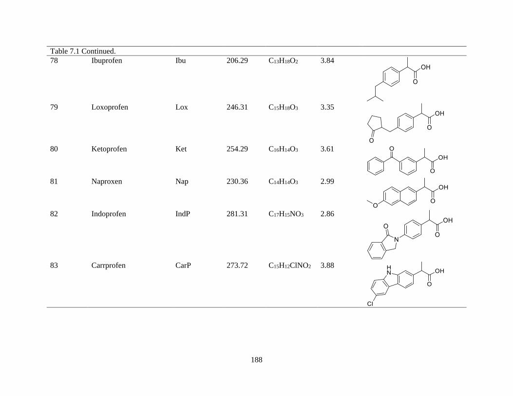
188


78 Ibuprofen Ibu 206.29 C13H18O2 3.84

79 Loxoprofen Lox 246.31 C15H18O3 3.35

80 Ketoprofen Ket 254.29 C16H14O3 3.61

81 Naproxen Nap 230.36 C14H14O3 2.99

82 Indoprofen IndP 281.31 C17H15NO3 2.86

83 Carrprofen CarP 273.72 C15H12ClNO2 3.88

189


84 Flurbiprofen FlBp 244.27 C15H13FO2 3.94

85 Fenoprofen FenP 242.27 C15H14O3 3.65

86 Aspirin Asp 180.16 C9H8O4 1.24

87 Salsalate Sal 258.23 C14H10O5 3.64

88 Diflunisal DifS 250.20 C13H8F2O3 3.91

89 Flufenamic acid FFen 281.23 C14H10F3NO2 5.25

90 Mefenamic acid MFen 241.29 C15H15NO2 5.40

190


91 Tolfenamic acid Tof 261.71 C14H12ClNO2 5.49

92 Diclofenac acid DCFen 296.15 C14H11Cl2NO2 4.26

93 Aceclofenac ACFen 354.18 C16H13Cl2NO4 3.88

94 Etodolac EtD 287.36 C17H21NO3 3.44

95 Oxaprozin OxA 293.32 C18H15NO3 3.46

96 Phenylbutazone PhBtz 308.38 C19H20N2O2 4.14

191


97 Nabumentone Nab 228.29 C15H16O2 3.22

98 Fenbufen FenB 254.29 C16H14O3 3.00

99 Nimesulide Nim 308.31 C13H12N2O5S 1.79

100 Piroxicam Pir 331.35 C15H13N3O4S 0.60

101 Meloxicam Mel 351.40 C14H13N3O4S2 1.60

192


102 Indometacin IndM 357.79 C19H16ClNO4 3.53

103 Sulindac Sul 356.41 C20H17FO3S 2.93

104 Acetaminophen AcTP 151.17 C8H9NO2 0.91

105 Phenacetin PhAct 179.22 C10H13NO2 1.41

193

7.2.2.2.2 Instrumentation


3080DG degasser, 3080MX high pressure mixer, 3177UV variable wavelength UV absorbance

detector, and LC-Net II/ADC from Jasco Inc. (Easton, MN) was used to evaluate the temperature

and solvent composition dependence of solute retention. Either a CO-2060 or CO-2067

thermostatted column compartments, also from Jasco, were used to regulate column temperature.

Data were acquired using ChromNAV version 1.19.3 software. Chromatograms were exported and

analyzed using a peak finding program written in MATLAB 2015a (MathWorks, Natick, MA).

7.2.2.2.3 Chromatographic conditions

Temperature-dependent retention factors for all solutes in Table 7.1 were measured on a series of

four new Waters Acquity BEH C18 (50 mm x 2.1 mm I.D., 1.7 μm dp) columns. The 105 solutes

were broken into four roughly equivalent groups and screened from 0.975:0.025 to 0.05:0.95 10

mM H3PO4/acetonitrile. Care was taken to group solutes from homologous series into the same

sample running them on the same column and batch of mobile phase when possible. Samples were

made in mobile phase at concentrations between 100 and 500 μM. Column temperature was varied

from 25 to 75 °C in 10 °C steps at each mobile phase composition using the CO-2060 oven and

25-65 °C using the CO-2067 oven. The CO-2067 column oven had a temperature maximum of 65

°C, thus the 75 °C runs were omitted. Mobile phase compositions tested ranged from 0.025 to 0.95

(w/w) acetonitrile/10 mM H3PO4 in 0.025 (w/w) acetonitrile steps from 0.025 to 0.10, then 0.05

(w/w) steps to 0.95 (w/w) acetonitrile. Each mobile phase was made by weight to improve

composition accuracy. Weight-to-weight aqueous-organic compositions were converted to

volume-to-volume units using density data provided by Billen et al. [88]. Detection at 100 Hz used

absorbance at 220 and 254 nm; injection volume was 5 μL. Flow rate was set to 0.35 mL/min.

194

Retention times were adjusted for extra column time determined using a Valco zero-dead-volume

union in place of the column.

7.2.2.2.4 Preliminary results: Nonlinear fitting to the Neue-Kuss equation

An equation designed by Neue and Kuss to model the influence of changes in solvent composition

and column temperature was fit to the raw retention data for all 105 test solutes [160]. This

equation is shown as Eq. 7.1:

ln 𝑘 = − ln 𝑘0,𝑇 +𝐷

𝑇+ 2 ln(1 + 𝑎𝜙) − (1 +

𝐷

𝑇)

𝐵𝑇𝜙

1 + 𝑎𝜙

(7.1)

where T is the temperature in Kelvin, φ is the volume-based mobile phase composition, a and D

are coefficients to express the influence of solvent and temperature and k0,T and BT are the

coefficients for retention in 100% water and the slope of the retention relationship with solvent

composition including temperature effects. Nonlinear curve fitting for each solute was performed

in Excel as described in Section 5.4.1. Results for all solutes are organized in Table 7.2. Fits for

all well retained solutes were good, with R2 values in excess of 0.9990. Fit quality did show a

strong correlation with mobile phase composition decreasing for both the high and low acetonitrile

compositions. This result was due to the small, but measurable retention of uracil under the highly

aqueous, <10% acetonitrile, and organic, >90% acetonitrile, conditions. We are in the process of

quantitatively addressing this problem.

195

Table 7.2. Curve fitting results for Neue-Kuss retention equation using the Waters Acquity BEH

C18 column as a function of temperature (25-65 °C) and solvent composition.

Index Analyte ln k0,T BT a D Fit (R2) na

1 Bz 2.38 1.14 0.38 2083 0.9993 260

2 1Bz 2.66 1.42 0.70 2674 0.9997 260

3 2Bz 2.87 1.52 0.80 3174 0.9995 280

4 3Bz 3.01 1.37 0.68 3466 0.9989 260

5 4Bz 3.14 1.15 0.47 3609 0.9984 260

6 5Bz 3.27 0.99 0.32 3741 0.9983 240

7 i4Bz 3.51 1.11 0.46 3700 0.9983 312

8 BzA 3.00 1.63 0.93 2054 0.9990 312

9 AP2 2.46 2.26 1.37 2150 0.9994 260

10 AP3 2.50 2.01 1.17 2547 0.9995 260

11 AP4 2.76 1.98 1.20 3059 0.9994 240

12 AP5 3.10 1.93 1.20 3600 0.9993 260

13 AP6 3.41 1.85 1.17 4085 0.9990 260

14 AP7 3.64 1.70 1.04 4418 0.9987 240

15 AP8 3.80 1.49 0.86 4588 0.9984 240

16 BA 4.24 2.20 1.53 2624 0.9993 240

17 Bz1 2.65 2.03 1.22 2542 0.9995 260

18 Bz2 2.78 2.05 1.27 3026 0.9994 240

19 Bz3 3.04 1.98 1.25 3527 0.9993 260

20 Bz4 3.28 1.89 1.20 3974 0.9991 260

21 hBzA 4.71 2.33 1.85 2354 0.9989 160

22 HP2 4.77 2.85 2.37 2605 0.9995 192

23 HP3 4.30 2.66 2.04 2892 0.9998 216

24 HP4 4.07 2.65 1.95 3259 0.9998 216

25 hBA 6.11 2.15 1.67 2639 0.9979 120

26 PB1 4.65 2.50 1.96 2902 0.9998 216

27 PB2 4.30 2.64 1.99 3270 0.9998 216

28 PB3 4.23 2.70 2.02 3770 0.9997 216

29 PB4 4.33 2.59 1.93 4252 0.9995 240

30 Ind 4.35 1.30 0.71 2836 0.9997 240

31 Inde 3.08 1.60 0.91 3116 0.9998 280

32 Naph 3.76 1.59 0.98 3573 0.9995 288

33 DPM 3.33 1.88 1.17 4258 0.9993 260

34 BPh 3.74 1.56 0.92 3936 0.9992 288

35 DPol 3.14 2.57 1.72 3368 0.9998 200

36 BzP 3.76 1.95 1.30 3723 0.9995 288

37 DPS 4.15 2.29 1.64 3629 0.9999 200

38 DPA 4.08 1.87 1.22 4083 0.9998 240

196


39 DPE 3.48 1.79 1.09 4037 0.9994 260

40 Car 4.60 2.06 1.49 4213 0.9998 220

41 BzPh 3.42 1.99 1.26 3971 0.9995 240

42 BzI 2.90 3.02 2.06 3234 0.9997 200

43 BzTan 3.31 2.09 1.29 3006 0.9997 220

44 BzAd 2.88 2.96 1.43 1647 0.9987 120

45 nBzAd 1.86 4.00 2.10 1510 0.9992 140

46 AcTan 2.66 2.86 1.69 1856 0.9990 160

47 TFT 2.70 1.83 1.03 3224 0.9996 240

48 FBz 2.43 1.31 0.52 2241 0.9994 260

49 dFBz 2.36 1.33 0.52 2320 0.9992 260

50 FBPh 3.32 1.93 1.21 4125 0.9993 260

51 NtBz 2.68 1.14 0.34 2093 0.9984 260

52 ClBz 2.67 1.45 0.71 2724 0.9995 280

53 dClBz 3.10 1.61 0.93 3418 0.9995 280

54 BzSA 4.18 2.20 1.52 2007 0.9977 140

55 Phenol 3.83 2.00 1.45 2185 0.9990 200

56 4MPh 3.78 2.23 1.56 2169 0.9998 180

57 ScA 4.75 1.87 1.33 2841 0.9989 220

58 VA 5.30 3.16 2.61 2638 0.9991 144

59 PhAA 4.06 2.16 1.42 2580 0.9994 240

60 HPhAA 6.63 2.82 2.63 3018 0.9988 144

61 2PhP 4.02 2.52 1.81 3062 0.9998 240

62 4MCN 3.59 1.78 1.11 2621 0.9997 240

63 Ans 3.04 1.33 0.64 2424 0.9996 312

64 BzO2 3.09 1.46 0.77 2847 0.9997 312

65 mNap 3.99 1.65 1.05 3731 0.9995 288

66 2NAA 4.84 2.96 2.36 4151 0.9996 216

67 PhAc 2.86 1.70 0.92 2319 0.9992 288

68 InAA 5.46 2.56 2.05 3303 0.9996 160

69 hInd 5.50 1.46 1.12 2400 0.9998 160

70 2HiP 2.56 3.38 1.77 1855 0.9998 140

71 4HiP 3.15 3.22 1.89 2322 0.9998 160

72 Caff 3.28 4.85 2.67 2084 0.9961 120

73 The 4.40 3.73 0.55 1941 0.9904 80

74 dClPy 1.58 1.39 0.46 1760 0.9986 300

75 ClQu 2.42 2.12 1.28 2624 0.9994 260

76 mnQu 1.78 2.22 1.13 1972 0.9973 260

77 Pan 4.71 2.82 2.20 4948 0.9997 220

78 Ibu 3.94 2.67 1.94 4857 0.9990 264

79 Lox 3.56 4.05 3.05 4239 0.9998 160

80 Ket 4.44 3.32 2.59 4658 0.9995 216

81 NaP 4.68 3.19 2.52 4678 0.9996 216

82 IndP 4.29 4.55 3.64 4867 0.9998 160

197


83 CarP 5.10 3.70 3.05 6108 0.9997 200

84 FlBp 4.08 3.44 2.65 5331 0.9997 200

85 FnP 4.13 3.26 2.49 5048 0.9997 200

86 Asp 4.32 2.96 2.24 2828 0.9997 216

87 Sal 4.71 2.94 2.29 4496 0.9999 200

88 DifS 5.14 2.99 2.42 5274 0.9998 220

89 FFen 4.43 2.95 2.24 5810 0.9994 220

90 MFen 4.44 2.71 2.06 5436 0.9992 240

91 Tof 4.53 2.47 1.85 5387 0.9991 220

92 DCFen 4.41 3.03 2.32 5307 0.9996 200

93 ACFen 4.64 3.21 2.50 5782 0.9996 200

94 EtD 3.48 3.30 2.43 4877 0.9994 220

95 OxA 3.61 4.12 3.19 5504 0.9995 200

96 PhBtz 3.26 2.51 1.67 4485 0.9992 220

97 Nab 3.73 2.59 1.85 4243 0.9996 220

98 FenB 4.49 3.58 2.83 5089 0.9998 180

99 Nim 5.04 2.34 1.73 4543 0.9998 200

100 Pir 2.29 4.15 2.90 3066 0.9991 200

101 Mel 4.05 3.37 2.61 4419 0.9996 200

102 IndM 4.39 3.37 2.62 5736 0.9994 200

103 Sul 4.52 6.00 4.92 6364 0.9996 140

104 AcTP 5.43 4.20 3.91 2281 0.9975 96

105 PhAct 2.89 3.39 2.27 2519 0.9998 216 aTotal number of experimental data points used in nonlinear curve fitting.

198

Panel A of Figure 7.5 shows simulated ln k versus φ curves using the four Neue-Kuss parameters

for each solute in Table 7.2. Column temperature was 70 °C. The degree of chemical diversity and

large number of solutes explains the high degree of overlap between all 105 curves. Panel B plots

a subset of 29 non-steroidal anti-inflammatory (NSAID) and over the counter pain relievers.

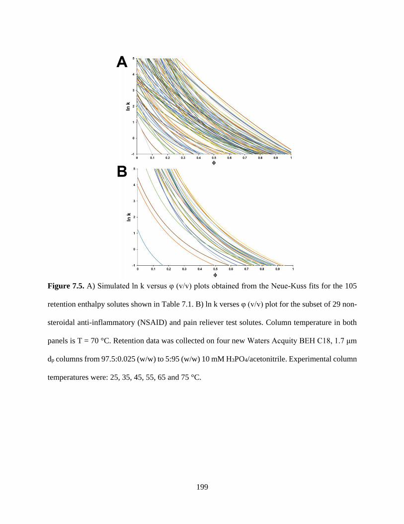
199

Figure 7.5. A) Simulated ln k versus φ (v/v) plots obtained from the Neue-Kuss fits for the 105

retention enthalpy solutes shown in Table 7.1. B) ln k verses φ (v/v) plot for the subset of 29 non-

steroidal anti-inflammatory (NSAID) and pain reliever test solutes. Column temperature in both

panels is T = 70 °C. Retention data was collected on four new Waters Acquity BEH C18, 1.7 μm

dp columns from 97.5:0.025 (w/w) to 5:95 (w/w) 10 mM H3PO4/acetonitrile. Experimental column

temperatures were: 25, 35, 45, 55, 65 and 75 °C.

200

7.2.2.2.5 Future work

Future work will include: 1) gather more retention data on different stationary phases and 2)

determine what additional information resides in the collected dataset. First, we will begin

collecting retention data for the same 105 solutes on two additional reversed phase materials. We

have selected a polar-embedded amide column (Supelco Ascentis Express RP-Amide) and a

pentafluorophenyl propyl phase (Supelco Ascentis Express F5). We have acquired five columns

of each phase from their manufacturer. From the data we have we will determine functional group

contributions to standard state retention enthalpies. We will apply the extrathermodynamic concept

expressed for free energies by the Martin equation. This concept states that retention enthalpy is

the sum of the enthalpies of retention from the individual fragments that comprise the molecule.

In creation of our 105-solute library we have taken care to select specific solutes that differ by only

one or a small number of molecular fragments. Thus, from the solvent and temperature dependent

retention data for a small number of test solutes we can elucidate a single molecular fragment’s

contribution to retention enthalpy. Our hope is to use this information to predict retention

enthalpies for compounds for which we have not collected retention data.

201

APPENDIX A

Supplemental Information for Chapter 2.

A1.1 van`t Hoff retention studies for parabens on Waters BEH C18 phase

Figure A1.1 shows the van’t Hoff plot generated for the four parabens tested under the conditions

outlined in Section 2.3.2.2. Plots were found to be linear over the temperature range evaluated for

samples run in triplicate after inspection of each regression’s residuals. Retention factors

calculated at 5 and 60 °C from the regression applied to Figure A1.1 are reported in Table A1.1.

Figure A1.1. van`t Hoff plot for methylparaben (●), ethylparaben (●), propylparaben (●), and

butylparaben (○) from 25 to 75 °C. For chromatographic conditions see section 2.3.2.2.

202

A1.2. TASF simulations, experimental details

A1.2.1 Influence of changes in focusing and separation temperature

The following discussion illustrates the series of relationships used to generate simulated

isothermal and TASF separations in silico. To model the potential for a hypothetical TASF analysis

the influence of column temperature on solute retention factor and reduced velocity must be known

accurately. The van`t Hoff equation was used to describe the relationship between solute retention

factor and column temperature:

ln 𝑘′ = −∆𝐻0

𝑅𝑇+

∆𝑆0

𝑅+ ln 𝜑

(A1.1)

where ∆𝐻0 is the standard state retention enthalpy, ∆𝑆0 is the standard state retention entropy, 𝑅

is the ideal gas constant and φ is the column phase ratio. From experimental plots of ln k’ vs. 1/T,

so-called van`t Hoff plots (Figure A1.1), retention factors were predicted at specific trapping and

separation temperatures.

Temperature’s influence on reduced velocity arises from reduced velocity’s inverse dependence

on solute diffusion coefficient. Diffusion coefficients are dependent on mobile phase viscosity and

temperature. An empirical relationship for viscosity as a function of composition and temperature

[26] was fit to the apparent integral viscosities at 400 bar for water-acetonitrile mixtures between

20 and 100 °C [88] resulting in:

𝜂(𝑇) = 10[−2.533+742𝑇⁄ −0.452𝑋𝐴𝐶𝑁+(235

𝑇⁄ )𝑋𝐴𝐶𝑁+1.573𝑋𝐴𝐶𝑁2 −(691

𝑇⁄ )𝑋𝐴𝐶𝑁2 ]

(A1.2)

203

Diffusion coefficients at various temperatures and mobile phase compositions were calculated

based on the following empirical equation [91]:

𝐷𝑚,𝑖(𝑇) = 𝐷𝑚,𝑖,𝑇′×𝑇×𝜂(𝑇′)

𝑇′×𝜂(𝑇)

(A1.3)

where the diffusion coefficient for solute 𝑖 at a given temperature (𝑇′) is known (𝐷𝑚,𝑖,𝑇′). Diffusion

coefficients for solutes used in TASF simulations are shown in Table A1.1.

Table A1.1. Experimental diffusion coefficients for each solute in water at 37 °C [87, 199] and

retention factors calculated from Table 1.2 at focusing and separation temperatures.

Solute Dm,37 °C (cm2/s) k’5 °C k’60 °C

Methylparaben 1.09×10-5 8.2 2.5

Ethylparaben 9.80×10-6 18.0 4.5

Propylparaben 9.06×10-6 70.2 15.3

Butylparaben 7.04×10-6 222.5 38.4

Uracilᵻ 9.34×10-6 - -

ᵻDiffusion coefficient measured at 30 °C and converted to 37 °C here using Eq. A1.3.

A1.2.2 Practical considerations of experimental setup

The physical size of the injection valve stator and associated fittings necessary to connect the

column to the valve creates a practical problem. Contained within this 18-20 mm segment of the

204

room temperature valve is stationary phase. The large size of the valve places a 2 cm long column

in front of the Peltier cooled trapping segment. Solutes must first be presented with the cooled

trapping segment upon initial interaction with the stationary phase for effective focusing. If not

analyte bands begin to separate on this 2 cm pre-column. If retention is high enough solutes may

not reach the trap before TEC polarity is reversed negating any potential benefit of the TASF

approach. To alleviate this problem experiments effectively removed this pre-column by leaving

it void of stationary phase. This exact solution to the problem of uncontrolled column temperature

within the injection valve was first proposed by Holm et al. [81] in their application of Peltier

based column cooling.

Introduction of the pre-column void is not without practical consequences. The void adds

significantly to the pre-column volume, >300 nL for the 150 μm I.D. columns used in this work,

introducing additional dispersion and making accurate calculations for solute residence time in the

trapping segment (𝑡𝑓𝑜𝑐𝑢𝑠) and observed retention time (𝑡𝑅,𝑖) more difficult. Due to the relatively

short length, 2 cm, and wide diameter of the pre-column void accurate determination of its

contribution to observed dispersion is difficult to model theoretically, i.e. it is not in the Taylor-

region. The following method was used to ascertain an approximate value for dispersion

introduced by the pre-column void used in TASF simulations. A series of three 45 nL, 60 °C

isothermal injections of methylparaben and ethylparaben were made and observed peak variances

and retention times were measured. Using the Knox equation the column variance (Eq. 1.10) at

reduced velocities of 3, 5 and 10 were estimated from the 𝐴, 𝐵, 𝐶, and 𝑛 coefficients in Table 2.3.

To account for a potentially more poorly packed column two 𝐷-coefficients were used in the

calculation, 0.42 and 0.6. Post-column dispersion was predicted from Taylor theory. Dispersion

due to the column and post-column were subtracted from the observed peak variances for

205

methylparaben and ethylparaben. A value for the isothermal time variance due to the pre-column

void (𝜎𝑡,𝑣𝑜𝑖𝑑,𝑖𝑠𝑜2 ) was estimated from the average of these six values and found to be 0.000571

min2.

To account for the time delay introduced by the pre-column dead volume the void time (tvoid) was

calculated as:

𝑡𝑣𝑜𝑖𝑑 =𝜋𝑎2𝐿𝑣𝑜𝑖𝑑

𝐹

(A1.4)

where 𝑎 is the column radius, 𝐿𝑣𝑜𝑖𝑑 is the length of the void, and 𝐹 is the volumetric flow rate.

The focusing time (𝑡𝑓𝑜𝑐𝑢𝑠) on column 1 is given by:

𝑡𝑓𝑜𝑐𝑢𝑠 = 𝑡𝑠 − 𝑡𝑣𝑜𝑖𝑑

(A1.5)

where 𝑡𝑠 is the time when TEC polarity is reversed, heating the focusing segment of the column

to the separation temperature. Retention times for retained solutes, 𝑡𝑅,𝑖, in TASF experiments were

calculated by summing the individual times required to progress through the fluidic system:

𝑡𝑅,𝑖 = 𝑡𝑖𝑛𝑗 + 𝑡𝑣𝑜𝑖𝑑 + 𝑡𝑓𝑜𝑐𝑢𝑠 + 𝑡𝑟𝑒𝑠,2 + 𝑡𝑝𝑜𝑠𝑡

(A1.6)

where 𝑡𝑖𝑛𝑗 is the injection time, 𝑡𝑣𝑜𝑖𝑑 is the void time, 𝑡𝑓𝑜𝑐𝑢𝑠 is the time the solute resides in the

trapping segment, 𝑡𝑟𝑒𝑠,2 is the time required to the solute to elute from the rest of the column, and

𝑡𝑝𝑜𝑠𝑡 is the time required to pass through the post column tubing.

206

Table A1.2 shows the 10 injection volumes used in simulated experiments.

Table A1.2. Values used for injection volume in simulations.

Injection Number Vinj (nL)

1 45

2 60

3 90

4 120

5 225

6 450

7 600

8 750

9 900

10 1050

Figure A1.2 shows simulated 5 and 45 nL injections in a hypothetical system without any pre-

column void, i.e. 𝜎𝑡,𝑣𝑜𝑖𝑑,𝑖𝑠𝑜2 = 0. Uracil concentration was reduced by a factor of 10 and 5 for the

5 and 45 nL injection simulations.

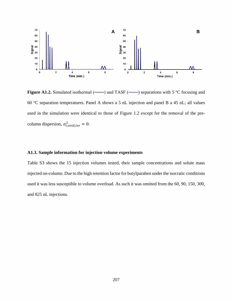
207

Figure A1.2. Simulated isothermal (───) and TASF (───) separations with 5 °C focusing and

60 °C separation temperatures. Panel A shows a 5 nL injection and panel B a 45 nL; all values

used in the simulation were identical to those of Figure 1.2 except for the removal of the pre-

column dispersion, 𝜎𝑡,𝑣𝑜𝑖𝑑,𝑖𝑠𝑜2 = 0.

A1.3. Sample information for injection volume experiments

Table S3 shows the 15 injection volumes tested, their sample concentrations and solute mass

injected on-column. Due to the high retention factor for butylparaben under the isocratic conditions

used it was less susceptible to volume overload. As such it was omitted from the 60, 90, 150, 300,

and 825 nL injections.

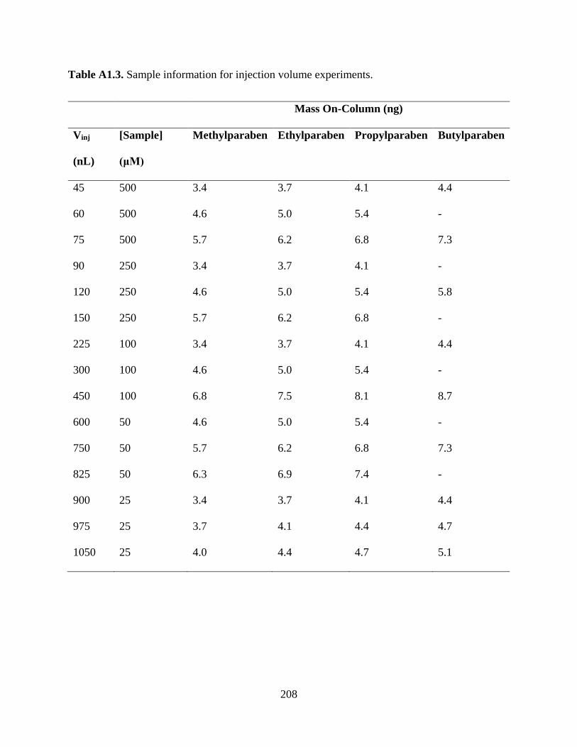
208

Table A1.3. Sample information for injection volume experiments.

Mass On-Column (ng)

Vinj

(nL)

[Sample]

(μM)

Methylparaben Ethylparaben Propylparaben Butylparaben

45 500 3.4 3.7 4.1 4.4

60 500 4.6 5.0 5.4 -

75 500 5.7 6.2 6.8 7.3

90 250 3.4 3.7 4.1 -

120 250 4.6 5.0 5.4 5.8

150 250 5.7 6.2 6.8 -

225 100 3.4 3.7 4.1 4.4

300 100 4.6 5.0 5.4 -

450 100 6.8 7.5 8.1 8.7

600 50 4.6 5.0 5.4 -

750 50 5.7 6.2 6.8 7.3

825 50 6.3 6.9 7.4 -

900 25 3.4 3.7 4.1 4.4

975 25 3.7 4.1 4.4 4.7

1050 25 4.0 4.4 4.7 5.1

209

APPENDIX B


B2.1. van`t Hoff retention studies for parabens on Waters BEH C18 phase

Solute retention factors were corrected for extra-column contributions to retention time using Eq.

B2.1:

𝑘′ = (𝑡𝑅 − 𝑡0

𝑡0 − 𝑡𝐸𝐶)

(B2.1)

where 𝑡𝑅 is solute retention time, 𝑡0 is the column void time and 𝑡𝐸𝐶 is the extra column void time.

The van`t Hoff equation was used to describe the relationship between solute retention factor and

column temperature:

ln 𝑘′ = −∆𝐻0

𝑅𝑇+

∆𝑆0

𝑅+ ln 𝜑

(B2.2)



so-called van`t Hoff plots (Figure. B2.1), retention factors were predicted at specific trapping and


Figure B2.1 shows the van’t Hoff plots generated for the four parabens under the conditions

outlined in Section 3.2.2.2. Plots were found to be linear over the evaluated temperature range for

210

samples run in triplicate after inspection of each regression’s residuals. Panels A-C shows results

for the 90:10, 80:20 and 70:30 10 mM H3PO4/acetonitrile mobile phases, respectively. Table B2.1

shows the results for the linear regressions applied to the van’t Hoff plots in Figure B2.1.

211

Figure B2.1. van`t Hoff plot for methylparaben (●), ethylparaben (●), and propylparaben (●) from

25 to 65 °C. Panels A-C shows results for the 90:10, 80:20 and 70:30 10 mM H3PO4/acetonitrile

mobile phases, respectively For chromatographic conditions see Section 3.2.2.2.

212

Table B2.1. Partial molar enthalpies of retention for methylparaben through propylparaben

obtained from slopes of the van`t Hoff plots in Figure B2.1. For chromatographic conditions see

Section 3.2.2.2.

ϕ Solute -ΔH°/R (K) Std Error Intercept Std Error

0.1


Ethylparaben 2611 23 -4.20 0.07


0.2


Ethylparaben 2205 32 -4.46 0.10


0.3


Ethylparaben 1667 21 -3.70 0.07


B2.2. TASF instrumentation

Figure B2.2 shows plots of temperature and pressure profiles collected from the TASF stability

study discussed in Section 3.3.2. The x-axis has been plotted to emphasize the first 90 s of a typical

TASF separation. The black dashed line has been placed at 35 s to indicate the focusing time, the

time when TEC temperature was changed from 𝑇1 to 𝑇2.

213

Figure B2.2. Column temperature (───) and pressure (───) profiles from TASF stability study

described in Section 3.3.2.

Figure B2.3 shows the long-term stability of the TASF instrumentation. Panel A shows this by

plotting the temperature (panel A) and pressure profiles (panel B) collected over the entire 975-

minute sequence. Temperature and pressure stability over the course of a 975-minute sequence

was good.

Figure B2.3. Column temperature (───) and pressure (───) profiles from TASF stability study

described in Section 3.3.2.

214

B2.3. Data Analysis

The MATLAB script used to determine peak FWHM values is provided below. The program

plotted each run, showing the selected baseline and FWHM for each peak. The file was input into

the MATLAB workspace as a single chromatogram containing the series of individual injections.

Data was first separated from a sequence of chromatograms into individual runs by factoring in

analysis run time. Each run was analyzed for peaks using the “findpeaks” command from the

MATLAB Signal Processing Toolbox. This command finds the local maxima within each data set

by specifying the minimum peak height and minimum distance between peaks. From the

maximum, the algorithm moves down the left and right sides of the peak to determine the baseline.

This is done by measuring the slope between two adjacent points 4 seconds apart until the slope

reaches or passes zero. The 4 second window was chosen so that algorithm would not stop at noise

and the point closest to the peak was used to determine the start of the baseline. The baseline was

then averaged on both sides of the peak. Once the baseline of the peak was determined, another

algorithm moved down from the peak maximum until it reached peak half height on either side

allowing FWHM measurement to be made. The minimum number of data points spanning a

FWHM in a single peak was 24 (FWHM = 0.92 s).

Visual inspection allowed for conformation of FWHM values. This program was fairly automated,

only requiring optimization of the following parameters: minimum peak height, distance between

peaks, length of run, slope thresholds and number of runs. The program allowed rapid analysis of

roughly 100 chromatograms containing 5 peaks each in about 20 seconds.

MATLAB Script:

clear

clf

hertz = 25;

load 2014-07-17-cgram.mat;

[columnlength,width] = size(cgram2);

215

%startingval shifts the window for chopping

startingval = 0;

startrun = 2;

numruns = 70;

%runlentest = 0, analysis; =1, no analysis

runlentest = 0;

%peakstart chooses what peak to start with for outputting the analysis

peakstart = 1;

peakendminus = 0;

runtime = 9.1;

for run = startrun:numruns;

lenrun = runtime*60*hertz;

choppeddatatime(:,run) = cgram2(startingval+run*lenrun-lenrun+1:startingval+run*lenrun,1);

choppeddataabs(:,run) = cgram2(startingval+run*lenrun-lenrun+1:startingval+run*lenrun,2);

if runlentest == 1

plot(choppeddatatime(:,run),choppeddataabs(:,run))

test = run

pause

clf

end

end

for run = startrun:numruns

%datacollectionrate

data(:,2) = choppeddataabs(:,run);

data(:,1) = choppeddatatime(:,run);

[pks,loc] = findpeaks(data(:,2),'minpeakheight',5,'minpeakdistance',900);

actualloc = loc/60/25

%number of peaks

numpeaks(run,:) = size(loc);

noisethresh = -0.000001

distthresh = 100

%find ends of peaks

for i=peakstart:numpeaks(run,1)-peakendminus

lft = loc(i)-800;

rgt = loc(i)+100;

while data(lft+distthresh,2) - data(lft,2) > noisethresh

lft = lft - 1;

end

left(i) = lft;

while data(rgt-distthresh,2) - data(rgt,2) > noisethresh

rgt = rgt + 1;

end

right(i) = rgt;

end

%baseline on each side of peaks

for i=peakstart:numpeaks(run,1)-peakendminus

leftbaseline = data(left(i)-50:left(i),2);

rightbaseline = data(right(i):right(i)+50,2);

peakbaselineavg(i,1) = mean(leftbaseline);

peakbaselineavg(i,2) = mean(rightbaseline);

end

%FWHM

for step = peakstart:numpeaks(run,1)-peakendminus

avgbaseline(step,1) = (peakbaselineavg(step,1)+peakbaselineavg(step,2))/2;

peakheight(step,1) = pks(step,1) - avgbaseline(step,1);

halfpeakheight(step,1) = peakheight(step,1)/2;

lft = loc(step)-1;

rgt = loc(step)+1;

while halfpeakheight(step,1) < (data(lft,2)-avgbaseline(step,1));

lft = lft - 1;

end

fwhmleft(step,1) = lft;

while halfpeakheight(step,1) < (data(rgt,2)-avgbaseline(step,1));

216

rgt = rgt + 1;

end

fwhmright(step,1) = rgt;

fwhm(1,step) = (fwhmright(step,1) - fwhmleft(step,1))/hertz/60;

end

plot(choppeddatatime(:,run),choppeddataabs(:,run))

xlabel('Time (min)')

ylabel('Absorbance (mAu)')

hold on

for i = peakstart:numpeaks(run,1)

p1 = [data(left(i),1),data(left(i),2)];

p2 = [data(right(i),1), data(right(i),2)];

plot([p1(1),p2(1)],[p1(2),p2(2)],'Color','r','LineWidth',0.5)

hold on

fwhm1 = [data(fwhmleft(i,1),1),data(fwhmleft(i,1),2)];

fwhm2 = [data(fwhmright(i,1),1),data(fwhmright(i,1),2)];

plot([fwhm1(1),fwhm2(1)],[fwhm1(2),fwhm1(2)],'Color','r','LineWidth',0.5)

hold on

end

fwhmminutes(run,1:numpeaks(run,1)) = fwhm(1:numpeaks(run,1))

test = run

pause

clf

end

217

B2.4. Second generation TASF instrumentation injection volume control experiments

Table B2.3 shows the 10 injection volumes tested, their sample concentrations and solute mass

injected on-column.

Table B2.2. Sample information for injection volume experiments.

Mass On-Column (ng)

Vinj (nL) [Sample] (μM) Methylparaben Ethylparaben Propylparaben

30 750 3.4 3.7 4.1

75 500 5.7 6.2 6.8

150 250 5.7 6.2 6.8

225 175 6.0 6.5 7.1

300 150 6.8 7.5 8.1

375 125 7.1 7.8 8.4

450 100 6.8 7.5 8.1

525 75 6.0 6.5 7.1

600 50 4.6 5.0 5.4

750 20 3.1 3.1 3.4

Figures B2.4 and B2.5 shows the results from the control experiments used to evaluate the

improved TASF system performance. See sections 3.2.3.4 and 3.3.3 for experimental details and

further discussion.

218

Figure B2.4. Example chromatograms from TASF separations of paraben samples made in mobile

phase. Isothermal (───) separations were performed at 70 °C. A 5 °C focusing temperature and

15 s focusing time were used with the TASF approach (───). Panel A shows the 30 nL injection,

panel B the 750 nL. For chromatographic conditions see Section 3.2.3.4.

219

Figure B2.5. Results from the injection volume experiments performed under isothermal (●) and

TASF (●) conditions with paraben mixtures made in mobile phase. Panels A, B, and C correspond

to methylparaben through propylparaben peaks, respectively. Isothermal separations are in black,

TASF in blue. Error bars were calculated using values for the standard error of each measured

FWHM, with n = 3. Red dashed lines are used to correspond to a 5% increase in peak width relative

to the 30 nL isothermal injection. A 5% increase in FWHM approximates a 10% reduction in

column efficiency. For chromatographic conditions see Section 3.2.3.4.

220

B2.5. Sample information for solvent- and temperature-based focusing injection volume

experiments

Table B2.4 shows the 5 injection volumes tested, their sample concentrations and solute mass

injected on-column.

Table B2.3. Sample information for injection volume experiments.

Mass On-Column (ng)

Vinj (nL) [Sample] (μM) Methylparaben Ethylparaben Propylparaben

100 300 4.6 5.0 5.4

500 100 7.6 8.3 9.0

1000 50 7.6 8.3 9.0

1500 35 8.0 8.7 9.5

2000 25 7.6 8.3 9.0

221

APPENDIX C


C3.1. Column Preparation

Capillary columns were prepared by packing Waters Acquity BEH C18, 1.7 µm particles

(Millford, MA) into 150 µm ID x 360 µm OD fused-silica capillaries from Polymicro

Technologies (Phoenix, AZ). Column frits were made by sintering 2 µm solid borosilicate spheres

(Thermo Scientific, Fremont, CA) into the end of the 20 cm long column blank. Frits were about

1 mm in length. Fritted column blanks were placed into an ultrahigh pressure column packing

fitting described previously [98]. The column packing fitting was connected to a high pressure

straight coupler (60-21HF4, High Pressure Equipment, Erie, PA) with an internal volume of about

100 µL. Particles were slurried in isopropanol at a concentration of 65 mg/mL and sonicated for

20 minutes prior to packing using the downward slurry method. A Haskel model DHSF-302

pneumatic amplification pump (Haskel, Burbank, CA) was used to pack the column at 18,500 psi

for 10 minutes. Acetone was used as the packing solvent. A defined length column was packed by

controlling the mass of particles loaded into the bomb. In this case 30 µL of the particle slurry was

used to pack the column blank to a length of 5.5 cm. Following initial packing with stationary

phase pump pressure was allowed to dissipate naturally. The remaining section of the column

blank was packed with 8 µm solid silica spheres (Thermo). Particles were slurried in a 50:50 (v/v)

mixture of isopropanol and water at a concentration of 100 mg/mL. This second section of the

222

capillary column was packed at 20,000 for an additional 10 minutes. The packed, dual segment

column was flushed with acetonitrile and the solid silica section was cut to 3.9 cm prior to use.

To determine extra column time accurately a second nominally identical column blank was packed

with only 8 µm solid silica spheres. This column consisted of every portion of the separation

column, 8 µm silica spheres, frit, and the connection capillary between the column outlet and the

detector. We refer to this column as the e-column. The e-column was packed at 1,500 psi for 10

minutes using the same procedure described above. Following packing the column was flushed

with acetonitrile and cut to 3.9 cm prior to use.

C3.2. Experimental setup

Figure C3.1 shows a block diagram describing how instrument control and timing was achieved.

Agilent OpenLab CDS ChemStation (rev. C.01.06) was used to control the instrumentation

indirectly and acquire data. ChemStation methods were set to collect data at 100 Hz using the

Agilent 1200 UIB (G1390B). The UIB was also used to send a ‘remote start’ signal via its internal

relays to an analog input channel of the National Instruments USB-6008 DAQ. A simple

LabVIEW VI was written to interpret this signal and immediately actuate the Valco C72-6676EH

6-port injection valve ‘beginning’ the chromatographic run. The valve was controlled using TTL

logic. The VI was designed to mimic a sequence table where a series of injections of various

injection volume (time) could be specified. The table was indexed by the remote signals sent from

the Agilent UIB. This configuration meant that a certain amount of discontinuity between the

detector time controlled by timers inside ChemStation and the UIB and valve actuation controlled

by LabVIEW timers was present. This resulted in a certain time lag between when data collection

began and when the injection valve was physically actuated.

223

Figure C3.1. Block diagram detailing the configuration for the instrument used in this work.

Figure C3.2 demonstrates the presence of the lag time between data collection and actuation

described above for retention experiments under two different mobile phase conditions. Mobile

phase composition in panels A and C was 25% (w/w) acetonitrile; B and D was 20% (w/w)

acetonitrile. Panels A and B show overlays from four consecutive 50 nL timed injections of 250

µM PB1, PB2, PB3 and uracil made in mobile phase. Panels C and D focus on the UV disturbances

introduced by valve actuation at the beginning of the run. UV disturbances, indicated by red

arrows, are highly reproducible from run-to-run. Disturbances were found to systematically drift

to longer retention times for injections made later in the LabVIEW injection sequence table.

Retention times for actuation disturbances for the four runs of panel A occurred at 1.41, 1.37, 1.41,

and 1.45 s, respectively. Data for these runs were collected early in the LabVIEW sequence table.

Disturbances for panel B occurred at 2.86, 2.88, 2.92, and 2.97 s and were collected later in the

injection sequence. To collect accurate k’ values the systematic difference (increase) in extra

column time for runs must be taken into account. Details regarding the procedure to handle this is

described below.

224

Figure C3.2. Influence of injection delay on observed retention times for UV disturbance peaks

due to injection valve actuation.

C3.3. Accurate determination of t0 and tec

In capillary liquid chromatography, the extra-column volume can be a significant fraction of the

total liquid volume between the injection loop and the optical path of the detector. Thus, the

determination of t0 is not trivial. We determined the extra-column volume by making a column

containing only extra-column volume, i.e., it does not have the stationary phase-containing portion

of the column. As Figure 4.1 shows, this column has the 8 µm solid silica spheres, the frit, and the

connecting tubing between the column outlet and the detector. For convenience, we will refer to

this as the e-column. Volumes were determined by injecting the unretained (assumed) solute uracil

into both the e-column and a column with the stationary phase-containing portion. The

chromatographic void volume was determined as the difference between the two volumes.

225

Retention factors, corrected for extra-column volume, were calculated using Eq. C3.1

𝑘′ =𝑡𝑅,𝑖 − 𝑡0

𝑡0 − 𝑡𝑒𝑐

(C3.1)

where tR,i is the retention time for solute i, t0 is the dead time for the column using uracil and an

unretained solute, and tec is the retention time correction for extra-column volume (extra-column

time).

Extra-column time was determined by performing a series of 20 replicate 50 nL injections of uracil

into the e-column. Mobile phase composition was 80:20 (w/w) 10 mM H3PO4/acetonitrile; flow

rate was set to 4 µL/min. Figure C3.3 shows the overlay of the 20 injections of 1 mM samples of

uracil made in mobile phase. Panel A shows the instrument contributions to the observed peak

profile for the 50 nL injections. Panel B focuses on the instrument induced peak tailing due to all

extra-column processes. Panel C clearly shows the presence of the UV disturbances produced by

valve actuation. Retention time reproducibility for these disturbances is clearly quite good.

226

Figure C3.3. Injection profiles for 20 consecutive 50 nL injections of 1 mM uracil onto a 3.9 cm

x 150 µm ID column packed with 8 µm solid silica spheres.

Retention factors under each mobile phase composition were calculated using the following

procedure. To correct for the time lag between data collection and valve actuation all signals, uracil

extra-column time injections and paraben injections under different mobile phase compositions,

were aligned using the first UV disturbance induced by valve actuation. A simple MATLAB script

(MathWorks, Natick, MA) was written to find the first UV disturbance (valley) then align all signal

vectors to the same disturbance in each respective chromatogram. Following alignment, a new

time axis beginning at the base of the valley was assigned to the signal vector. The ‘findpeaks’

function was then used to find the local maxima and retention times for each peak. Finally,

retention factors were calculated by substituting the retention times (tR,i and t0) output by the

MATLAB script and a value of 0.147 minutes (the average aligned extra-column time, n = 20, σtec

= 0.0004 min., %RSD = 0.3%) for tec in Eq C3.1.

227

C3.4. Accurate calculation of k’

To further address potential inaccuracies in values for k’ retention factors were calculated k’ based

on solute retention time at peak maximum and each peak’s first central moment. Table C3.1 shows

the results from these calculations (n = 4). While small differences in k’ are present under each

condition when both datasets are used individual to create Figure 4.8 no significant difference in

the magnitude of tobs/tinj or the slope of the tobs/tinj vs k2/k1 is observed. Note that retention factors

calculated based on moments are smaller, not larger (as expected), than those determined using

time at peak maxima. This is due to the first moment calculated for uracil peaks. Uracil retention

under experimental conditions is minimal. Thus peak shape is significantly influenced by the

injector effects and connections between capillaries. Both combine to increased peak tailing for

uracil relative to retained solutes. Increased peak tailing increases the magnitude of the first

moment for the void marker leading to a reduction in calculated retention factor.

Table C3.1. Paraben retention factors calculated using time at peak maxima (tR,max) and first

central moments (μ1).

φ

0.2 0.1 0.05

Solute

k' σk k' σk k' σk

PB1 tR,max 2.06 0.017 7.02 0.02 15.89 0.04

μ1 1.93 0.04 6.56 0.13 15.06 0.2

PB2 tR,max 4.62 0.032 19.62 0.05 50.28 0.13

μ1 4.34 0.07 18.4 0.3 47.6 0.7

PB3 tR,max 10.82 0.08 57.56 0.2 - -

μ1 10.18 0.16 54 0.9 - -

228

C3.5. Open-tube injection analysis

As an instrument control and to demonstrate the ability to reproducibility for injections up to 2000

nL using the 75 cm x 75 μm ID nanoViper (V = 3.3 uL) injection loop a series of timed injections

were made into a 35 cm x 25 μm ID capillary connecting the injection valve directly to the detector

flow cell. Mobile phase composition was 80:20 10 mM H3PO4/acetonitrile, flow rate was set to 4

μL/min and data was collected at 100 Hz by monitoring UV absorbance at 254 nm. The sample

was 1 μM uracil in mobile phase. Injections were made from 250 nL to 2500 nL in 250 nL steps.

Order of large volume injections was random and a 50 nL injection of the uracil sample was made

between every large volume injection. Figure S4A shows an overlay for all ten injections in black

with the 50 nL injection in red.

Figure C3.4. Panel A shows injection profiles obtained from time injections from 250 to 2500 nL

(black) of 1 µM uracil into a 25 µm ID capillary. The red trace represents the profile obtained

when using a 50 nL injection. Panel B shows a plot of injection plug width versus injection volume.

Performing a series of injections into an open tube serves as a good control for the LabVIEW VI,

its timers used to control the injection valve, injection time and subsequently the injection volume

229

delivered to the column. Timed injections were used in all experiments. Thus, as equation C3.2

shows, the width of the injection band in time units, tinj, is the desired injection volume, Vinj, over

the volumetric flow rate, F, delivered by the pump. If the system (LabVIEW timers, injection

valve, and pump) are performing as designed and delivering appropriate length (volume) injections

the injection time should equal the width of the injection band at the detector, w1/2.

𝑡𝑖𝑛𝑗 = 𝑤1/2 =1

𝐹𝑉𝑖𝑛𝑗

C3.2

A plot of measured width versus injection time should be linear and have a slope equal to the one.

This plot is show in panel B of Figure C3.4. The equation from the linear regression was y = 1.0058

± 0.0075x – 0.0039 ± 0.0029 (95% confidence interval). The slope of the linear regression yielded

an experimentally determined flow rate of 3.977 ± 0.030 not significantly different from 4 µL/min,

the set value at the 95% confidence level. Thermo/Dionex does not provide a specification for flow

rate accuracy for the pump used, although we conclude the value of 0.5% to be quite good and will

not influence the results of our work.

C3.6. Non on-column focusing instrument control

A second instrument validation test was performed using a series of large volume injections with

samples made in mobile phase. For samples made in mobile phase any focusing of the sample

band induced by retention at the head of the column due to retention will be reversed as the band

expands at the column outlet. For large injections injection time (volume) and measure band width

are directly related.

230

Panel A of Figure C3.5 shows a series of 50 µM paraben injections from 250 to 1500 nL in 250

nL steps onto a 150 µm x 5.5 cm BEH C18, 1.7 µm dp column. Samples were made in 80:20 (wt%)

10 mM H3PO4/acetonitrile. Mobile phase composition was also 80:20 (wt%) 10 mM

H3PO4/acetonitrile. Flow rate was set to 4 µL/min and column temperature was 60 ºC.

Panel B shows the linear increase in peak width (in time units) with injection volume for all three

solutes. The dashed line with slope equal to one has been added to highlight the direct, as expected,

relationship between the two variables. Note that only the point for the 250 nL injection for PB3

shows any visible deviation from the linear increase between injection volume and peak width.

After performing regression calculations residuals plots clearly showed width values for the 250

nL injections for each solute had significant contributions due to on-column bandspreading. As

such the 250 nL points were excluded from the linear regression performed for all three solutes.

(Note that for smaller injection volumes on-column convective dispersion begins to contribute a

significant fraction of the observed to peak width, i.e. the injection volume is no longer volume

overloading the column under the experimental conditions.) The slope and intercept for the linear

regression were 0.992 ± 0.006 and -0.008 ± 0.002 (95% confidence interval), respectively.

Deviations from the predicted value of 1.0 while significant, are only 2% and represent an

acceptable error.

231

Figure C3.5. Injections of 250 to 1500 nL of 50 mM PB1, PB2, and PB3 made in mobile phase

onto 150 μm x 5.5 cm BEH C18 column. Panel B shows a plot of measured peak width versus

injection time for PB1 (●), PB2 (●), PB3 (●). To add clarity, the dashed line represents a line with

unit slope and intercept at the origin. For chromatographic conditions see Section 4.3.3.

C3.7. Effect of sample solvent composition and volume on peak shape

Figure C3.6 shows the chromatograms obtained from 500 (black), 1000 (red), 1500 (blue), and

2000 nL (purple) injections of PB1, PB2 and PB3 made in 90:10 (wt%) 10 mM H3PO4/acetonitrile.

These are provided to the reader with the complete chromatograms referenced in Section 4.4.3 and

Figure 4.6.

232

Figure C3.6. Effect of injection volume of peak shape for samples of PB1, PB2, and PB3 made in

90:10 (w/w) 10 mM H3PO4/acetonitrile injected into a mobile phase consisting of 80:20 (w/w) 10

mM H3PO4/acetonitrile.

Figure C3.7 shows similar chromatograms obtained from 500 (black), 1000 (red), 1500 (blue), and

2000 nL (purple) injections of PB1, PB2 and PB3 made in 95:5 (wt%) 10 mM H3PO4/acetonitrile.

These are provided to the reader with the complete chromatograms referenced in Section 4.4.3 and

Figure 4.6.

233

Figure C3.7. Effect of injection volume of peak shape for samples of PB1, PB2, and PB3 made in

95:5 (wt%) 10 mM H3PO4/acetonitrile injected into a mobile phase consisting of 80:20 (wt%) 10

mM H3PO4/acetonitrile.

C3.8. Plot of focusing data vs the independent variable (k2+1)/(k1+1)

A reviewer suggested that we plot the observed focusing factors vs the variable (k2+1)/(k1+1). This

is equivalent to testing the assumption that there is no step (or “steep”) gradient compression of

the injected zone. Figure C3.8 shows that the data (red circles): 1) do not lie on a straight line and

2) are consistently lower than the hypothetical result (black line) by significant and variable

relative quantities. While the information in Figure C3.8 is the same as that in Figure 4.8, it is

perhaps clearer in Figure C3.8 than in Figure 4.8 that on-column compression is a significant factor

in the overall focusing phenomenon in solvent-based focusing/isocratic elution.

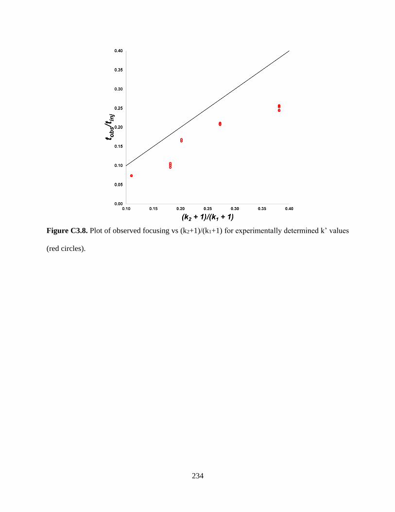
234

Figure C3.8. Plot of observed focusing vs (k2+1)/(k1+1) for experimentally determined k’ values

(red circles).

235

APPENDIX D


D4.1. Temperature and solvent composition dependence of retention factors

Values for retention factors for each solute were calculated based on their retention time and that

of uracil to approximate the void time, t0. Extra column time, tec, was measured by placing a Valco

ZDV union in place of the column. Eq. D4.1 was used to calculate retention factors while

accounting for the extra column time:

𝑘′ = 𝑡𝑅,𝑖 − 𝑡0

𝑡0 − 𝑡𝑒𝑐

(D4.1)

The van`t Hoff equation was used to describe the relationship between solute retention factor and

column temperature:

ln 𝑘′ = −∆𝐻0

𝑅𝑇+

∆𝑆0

𝑅+ ln 𝜑

(D4.2)



236

so-called van`t Hoff plots (Figure D4.1), retention factors were predicted at specific trapping and


237

Figure D4.1 van`t Hoff plots for parabens (●) p-hydroxyphenones (●). Mobile phase

compositions: 0.05 w/w (A), 0.10 (B), 0.15 (C), 0.20 (D), 0.25 (E), 0.30 (F), 0.35 (G), 0.40 (H),

0.45 (I), 0.50 (J), 0.55 (K), 0.60 (L). For chromatographic conditions see section 5.2.3.1.

238

Table D4.1. Partial molar enthalpies of retention for each solute used in retention studies obtained

from slopes of the van`t Hoff plots shown in Figure D4.1.

Solute φ (w/w) φ (v/v) -ΔH°/R (K) Error Intercept Error

p-Hydroxyacetophenone 0.050 0.063 2335 16 -5.07 0.05

0.100 0.124 1902 9 -4.54 0.03

0.150 0.184 1555 9 -4.10 0.03

0.200 0.242 1312 8 -3.83 0.03

0.250 0.299 1165 9 -3.75 0.03

0.300 0.354 1095 7 -3.84 0.02

p-Hydroxypropiophenone 0.050 0.063 2602 24 -4.64 0.07

0.100 0.124 2193 15 -4.30 0.05

0.150 0.184 1830 14 -3.91 0.04

0.200 0.242 1543 13 -3.62 0.04

0.250 0.299 1344 13 -3.48 0.04

0.300 0.354 1221 11 -3.49 0.03

0.350 0.407 1149 8 -3.59 0.03

0.400 0.460 1124 6 -3.79 0.02

p-Hydroxybutyrophenone 0.100 0.124 2459 22 -4.09 0.07

0.150 0.184 2090 19 -3.80 0.06

0.200 0.242 1770 17 -3.51 0.05

0.250 0.299 1522 17 -3.31 0.05

0.300 0.354 1352 15 -3.26 0.05

0.350 0.407 1243 13 -3.32 0.04

239

Table D4.1 Continued.

0.400 0.460 1190 11 -3.50 0.03

0.450 0.511 1148 9 -3.66 0.03

0.500 0.561 1117 7 -3.83 0.02

Methylparaben 0.050 0.063 2599 24 -4.89 0.07

0.100 0.124 2254 13 -4.69 0.04

0.150 0.184 1909 11 -4.32 0.03

0.200 0.242 1624 10 -4.02 0.03

0.250 0.299 1421 10 -3.85 0.03

0.300 0.354 1309 9 -3.87 0.03

0.350 0.407 1233 7 -3.95 0.02

0.400 0.460 1204 5 -4.13 0.02

Ethylparaben 0.100 0.124 2492 20 -4.37 0.06

0.150 0.184 2122 17 -4.06 0.05

0.200 0.242 1794 15 -3.73 0.05

0.250 0.299 1542 15 -3.51 0.05

0.300 0.354 1390 14 -3.50 0.04

0.350 0.407 1275 12 -3.53 0.04

0.400 0.460 1224 9 -3.70 0.03

0.450 0.511 1167 7 -3.81 0.02

0.500 0.561 1139 5 -3.97 0.02

Propylparaben 0.150 0.184 2473 20 -4.16 0.06

0.200 0.242 2093 18 -3.79 0.06

240

Table D4.1 Continued.

0.250 0.299 1780 19 -3.49 0.06

0.300 0.354 1573 18 -3.40 0.05

0.350 0.407 1408 17 -3.35 0.05

0.400 0.460 1328 14 -3.49 0.04

0.450 0.511 1247 12 -3.58 0.04

0.500 0.561 1209 10 -3.75 0.03

0.550 0.609 1141 8 -3.82 0.02

Butylparaben 0.200 0.242 2436 21 -3.98 0.07

0.250 0.299 2064 22 -3.60 0.07

0.300 0.354 1803 21 -3.43 0.07

0.350 0.407 1586 21 -3.30 0.07

0.400 0.460 1474 19 -3.41 0.06

0.450 0.511 1367 17 -3.46 0.05

0.500 0.561 1317 14 -3.65 0.04

0.550 0.609 1243 12 -3.73 0.04

0.600 0.657 1237 13 -3.99 0.04

Figure D4.3 shows Neue-Kuss fits to experimental retention data for the parabens and

hydroxyphenones in red and blue, respectively. Panels A, B, C, D, E and F correspond to column

temperatures of 25, 35, 45, 55, 65 and 75 °C. Fitting parameters are provided in Table 5.1.

241

Figure D4.2 Overlay of Neue-Kuss curve fitting results with experimentally determined retention

factors for parabens (●) p-hydroxyphenones (●). Column temperature: 25 (A), 35 (B), 45 (C), 55

(D), 65 (E), 75 °C (F). For chromatographic conditions see section 5.2.3.1.

242

D4.2. Characterization of two-stage TASF instrument performance

Figure D4.3 shows temperature profiles for TEC A (red), B (blue) and C (black) (panels A and B)

and temperature rate-of-change profiles (C and D) for the transient portions of Figure 5.2. The

temperature change was from 5 to 70 °C.

Figure D4.3 Temperature (A, B) and temperature ROC (C, D) profiles for transient

heating/cooling sections of Figure 5.2. TEC A is shown in red, TEC B blue, TEC C black.

243

D4.3. Simulating two-stage temperature-based focusing

Chromatographic conditions not reported in section 5.4.3 for isothermal, TASF and two-stage

TASF simulations are provided in Tables D4.2 and D4.3. Table D4.2 lists parameters used in the

isocratic simulations, D4.3 gradient elution parameters.

Table D4.2. Parameters used in isocratic isothermal, TASF and two-stage TASF simulations.

Parameter Value

Sample

Vinj (nL) 1500

φsample (v/v) 0.242 (0.2 w/w)

Temperature Program

T1,A; T1,B (°C) 5, 70

T2,A; T2,B (°C) 5, 70

Tcol (°C) 70

tfocus,A (s) 35

tfocus,B (s) 35, 60

Column Conditions

φ 0.242

L (cm) 8.0

dc (um) 150

F (uL/min.) 3

εe 0.38

εtot 0.56

dp (μm) 1.7

A (dimensionless van Deemter) 0.66

B 10.2

C 0.095

244

Table D4.3. Parameters used in gradient elution isothermal, TASF and two-stage TASF

simulations.

Parameter Value

Sample

Vinj (nL) 3000

φsample (v/v) 0.05

Temperature Program

T1,A; T1,B (°C) 5, 70

T2,A; T2,B (°C) 5, 70

Tcol (°C) 70

tfocus,A (s) 65

tfocus,B (s) 65, 100

Gradient Conditions

φinitial 0.05

φfinal 0.45

tdwell (s) 15

tg (s) 960

L (cm) 8.0

dc (um) 150

F (uL/min.) 3

εe 0.38

εtot 0.56

dp (μm) 1.7

A (dimensionless van Deemter) 0.66

B 10.2

C 0.095

D4.4. Two-stage TASF experiments: Gradient elution

Raw, non-baseline subtracted chromatograms are provided in Figure D4.3. Note in the raw signals

for the TASF and two-stage TASF runs exhibit large system peaks visible just after 2 minutes in

the TASF run and two transient peaks between 2 and 3 minutes in the two-stage experiments.

These transients correspond to the changes in column temperature and we believe they are due to

additional acetonitrile partitioning into the cold sections of the column. Following heating the

245

acetonitrile concentration in the stationary phase stabilizes, but heating releases a bolus of ACN

rich mobile phase leading to a change in the refractive index observed at the detector.

Figure D4.4 Example non-baseline subtracted gradient elution chromatograms under isothermal

(black), TASF (blue) and two-stage TASF (red) conditions. Baseline signals under each condition

are shown in gray.

246

D4.5. Simulation/Experiment Comparison

Figures D4.5 and D4.6 show qualitative comparisons of experimental and simulated

chromatograms collected under isocratic and gradient elution conditions for each temperature

program, isothermal (black), TASF (blue) and two-stage TASF (red).

Figure D4.5 Simulated (A) and experimental chromatograms (B) collected for isocratic

separations of paraben samples under isothermal (black), TASF (blue) and two-stage TASF (red)

conditions.

247

Figure D4.6 Simulated (A) and experimental chromatograms (B) collected using solvent gradient

elution conditions for the separation of paraben and p-hydroxyphenone samples under isothermal

(black), TASF (blue) and two-stage TASF (red) conditions.

248

APPENDIX E


E5.1 Historical Plots Used for Chromatographic Optimization

Figure E5.1 shows the initial kinetic plot presented by Giddings to compare the separation time in

gas and liquid chromatography [167].

Figure E5.1. Reproduced from Giddings, J. C. Anal. Chem. 1964, 36, 1890–1892. Copyright 1964

American Chemical Society.

249

Figure E5.2 is taken from Knox and Saleem to show the range of velocities presented to explore

the limits of liquid chromatography [168].

Figure E5.2. Reproduced from Knox, J. H.; Saleem, M. J. Chromatogr. Sci. 1969, 7, 614–622,

Copyright 1969, with permission from Oxford University Press.

Figure E5.3 is the first example of the Poppe plot [173].

250

Figure E5.3. Reprinted from the J. Chromatogr. A, Vol. 778, Poppe, H. Some reflections on speed

and efficiency of modern chromatographic methods, pp. 3 – 21. Copyright 1997, with permission

from Elsevier.

Figure E5.4 is a graphical representation of Kinetic Plot Method from Desmet et al. [183]. The

plot in the red square shows the fully transformed H vs u0 data.

251

Figure E5.4. Reproduced from Desmet, G.; Clicq, D.; Gzil, P. Analytical Chemistry 2005, 77,

4058–4070. Copyright 2005 American Chemical Society.

252

Figure E5.5 is the nomogram developed by Guiochon to determine the minimum analysis time to

achieve a desired number of theoretical plates [172].

Figure E5.5. Reprinted from High-Performance Liquid Chromatography Advances and

Perspectives Vol. 2, Guiochon, G. Optimization in Liquid Chromatography, pp. 1 – 56. Copyright

1980, with permission from Elsevier.

253

Figure E5.6 is the Halasz and Görlit [186] nomogram to estimate laboratory conditions under

similar conditions to Guiochon.

Figure E5.6. Reproduced from Optimale Parameter in der schnellen

Fluessigkeitschchromatographie (HPLC), Halász, I.; Görlitz, G. Angew. Chem. 1982, 94, 50–62 .

Copyright 1982 Wiley.

254

E5.2 Equations Used for Chromatographic Optimization

The value for serotonin’s diffusion coefficient measured in water at 25 °C, 5.4×10-6 cm2/s [190],

was translated to various temperatures and mobile phase compositions using the following

empirical equation [99]:

𝐷𝑚,𝑖(𝑇) = 𝐷𝑚,𝑖,𝑇′×𝑇×𝜂(𝑇′)

𝑇′×𝜂(𝑇)

(E5.1)

where Dm,T’ is the measured diffusion coefficient at a given temperature (T’), n(T’) is the viscosity

under those conditions, T is the desired temperature, and η(T) is the viscosity at the desired

composition and temperature.

An empirical relationship for viscosity as a function of composition and temperature was fit to the

apparent integral viscosities at 400 bar for water-acetonitrile mixtures between 20 and 100 °C

resulting in [26, 88]:

𝜂(𝑇) = 10[−2.533+742𝑇⁄ −0.452𝑋𝐴𝐶𝑁+(235

𝑇⁄ )𝑋𝐴𝐶𝑁+1.573𝑋𝐴𝐶𝑁2 −(691

𝑇⁄ )𝑋𝐴𝐶𝑁2 ]

(E5.2)

where T is the temperature in Kelvin and XACN is the volume fraction of acetonitrile and water.

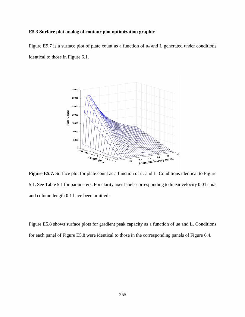
255

E5.3 Surface plot analog of contour plot optimization graphic

Figure E5.7 is a surface plot of plate count as a function of ue and L generated under conditions

identical to those in Figure 6.1.

Figure E5.7. Surface plot for plate count as a function of ue and L. Conditions identical to Figure

5.1. See Table 5.1 for parameters. For clarity axes labels corresponding to linear velocity 0.01 cm/s

and column length 0.1 have been omitted.

Figure E5.8 shows surface plots for gradient peak capacity as a function of ue and L. Conditions

for each panel of Figure E5.8 were identical to those in the corresponding panels of Figure 6.4.

256

Figure E5.8 Gradient peak capacity surface plots as a function of ue, t0 and tG for gradient times:

1, 3, 20, 60 minutes. Conditions identical to Figure 6.1. For clarity axes labels corresponding to

linear velocity 0.01 cm/s and column length 0.1 have been omitted.

E5.3 Statistical peak overlap theory calculations

Values for peak capacity required to resolve a predetermined number of unknown compounds, m,

with a desired probability, P1, of resolution as single component bands were calculated using

equation E5.3 [198]:

𝑃1 = exp (−2𝑚

𝑛𝑐)

(E5.3)

257

Figure E5.9 shows the peak capacity required to separate m sample constituents with a 90 (blue)

and 95% (black) probability of observing pure, single component peaks.

Figure E5.9 Peak capacity required to resolve samples composed of m constituents with a 90

(blue) and 95% (black) probability of observing each as a single pure peak.

258

BIBLIOGRAPHY

[1] A.J.P. Martin, R.L.M. Synge, A new form of chromatogram employing two liquid phases. I. A

theory of chromatography. Ii. Application to the microdetermination of the higher monoamino

acids in proteins, Biochem. J., 35 (1941) 1358-1368.

[2] B.L. Karger, L.R. Snyder, C. Horváth, An introduction to separation science, Wiley, New York,

1973.

[3] J. van Deemter, F. Zuiderweg, A. Klinkenberg, Longitudinal diffusion and resistance to mass

transfer as causes of nonideality in chromatography, Chemical Engineering Science, 5 (1956) 271-

289.

[4] P.R. Kasten, L. Lapidus, N.R. Amundson, Mathematics of adsorption in beds. V. Effect of

intraparticle diffusion in flow systems in fixed beds, J. Phys. Chem., 56 (1952) 683-688.

[5] L. Lapidus, N.R. Amundson, Mathematics of adsorption in beds. Vi. The effect of longitudinal

diffusion in ion-exchange and chromatographic columns, J. Phys. Chem., 56 (1952) 984-988.

[6] J.C. Giddings, Maximum number of components resolvable by gel filtration and other elution

chromatographic methods, Analytical Chemistry, 39 (1967) 1027-1028.

[7] U.D. Neue, Theory of peak capacity in gradient elution, Journal of Chromatography A, 1079

(2005) 153-161.

[8] Y. Ishihama, Proteomic lc–ms systems using nanoscale liquid chromatography with tandem

mass spectrometry, Journal of Chromatography A, 1067 (2005) 73-83.

[9] G. Theodoridis, H.G. Gika, I.D. Wilson, Lc-ms-based methodology for global metabolite

profiling in metabonomics/metabolomics, TrAC Trends in Analytical Chemistry, 27 (2008) 251-

260.

259

[10] L.A. Filla, W. Yuan, E.L. Feldman, S. Li, J.L. Edwards, Global metabolomic and isobaric

tagging capillary liquid chromatography–tandem mass spectrometry approaches for uncovering

pathway dysfunction in diabetic mouse aorta, Journal of Proteome Research, 13 (2014) 6121-6134.

[11] X. Gao, Q. Zhang, D. Meng, G. Isaac, R. Zhao, T.L. Fillmore, R.K. Chu, J. Zhou, K. Tang,

Z. Hu, R.J. Moore, R.D. Smith, M.G. Katze, T.O. Metz, A reversed-phase capillary ultra-

performance liquid chromatography–mass spectrometry (uplc-ms) method for comprehensive top-

down/bottom-up lipid profiling, Analytical and Bioanalytical Chemistry, 402 (2012) 2923-2933.

[12] W.E. Haskins, Z. Wang, C.J. Watson, R.R. Rostand, S.R. Witowski, D.H. Powell, R.T.

Kennedy, Capillary lc−ms <sup>2</sup> at the attomole level for monitoring and discovering

endogenous peptides in microdialysis samples collected in vivo, Analytical Chemistry, 73 (2001)

5005-5014.

[13] Y. Zhou, O.S. Mabrouk, R.T. Kennedy, Rapid preconcentration for liquid chromatography–

mass spectrometry assay of trace level neuropeptides, Journal of The American Society for Mass

Spectrometry, 24 (2013) 1700-1709.

[14] Y. Zhou, R.T. Kennedy, Capillary liquid chromatography-mass spectrometry detection of

trace level neuropeptides, 41st International Symposium on High Performance Liquid Phase

Separations and Related Techniques, (2014).

[15] Y. Zhou, J.-M.T. Wong, O.S. Mabrouk, R.T. Kennedy, Reducing adsorption to improve

recovery and in vivo detection of neuropeptides by microdialysis with lc-ms, Analytical

Chemistry, 87 (2015) 9802-9809.

[16] K. Maes, G. Béchade, J. Van Schoors, Y. Van Wanseele, J. Van Liefferinge, Y. Michotte,

S.N. Harden, E.E. Chambers, J. Claereboudt, I. Smolders, A. Van Eeckhaut, An ultrasensitive nano

260

uhplc–esi–ms/ms method for the quantification of three neuromedin-like peptides in

microdialysates, Bioanalysis, 7 (2015) 605-619.

[17] K. Maes, J. Van Liefferinge, J. Viaene, J. Van Schoors, Y. Van Wanseele, G. Béchade, E.E.

Chambers, H. Morren, Y. Michotte, Y. Vander Heyden, J. Claereboudt, I. Smolders, A. Van

Eeckhaut, Improved sensitivity of the nano ultra-high performance liquid chromatography-tandem

mass spectrometric analysis of low-concentrated neuropeptides by reducing aspecific adsorption

and optimizing the injection solvent, Journal of Chromatography A, 1360 (2014) 217-228.

[18] M.V. Novotny, I. Daido, Microcolumn separations columns, instrumentation, and ancillary

techniques, Elsevier ; Distributors for the U.S. and Canada, Elsevier Science Pub. Co., Amsterdam;

New York; New York, 1985.

[19] J.C. Sternberg, Advances in chromatography, 2 (1966) 205-270.

[20] S.R. Groskreutz, S.G. Weber, Quantitative evaluation of models for solvent-based, on-column

focusing in liquid chromatography, Journal of Chromatography A, 1409 (2015) 116-124.

[21] L.R. Snyder, Principles of gradient elution, Chromatographic Reviews, 7 (1965) 1-51.

[22] L.R. Snyder, D.L. Saunders, Optimized solvent programming for separations of complex

samples by liquid-solid adsorption chromatography in columns, Journal of Chromatographic

Science, 7 (1969) 195-208.

[23] A. Prüß, C. Kempter, J. Gysler, T. Jira, Extracolumn band broadening in capillary liquid

chromatography, Journal of Chromatography A, 1016 (2003) 129-141.

[24] J. Vissers, A. Deru, M. Ursem, J. Chervet, Optimised injection techniques for micro and

capillary liquid chromatography, Journal of Chromatography A, 746 (1996) 1-7.

261

[25] M.D. Foster, M.A. Arnold, J.A. Nichols, S.R. Bakalyar, Performance of experimental sample

injectors for high-performance liquid chromatography microcolumns, Journal of Chromatography

A, 869 (2000) 231-241.

[26] D. Guillarme, S. Heinisch, J.L. Rocca, Effect of temperature in reversed phase liquid


[27] J.D. Thompson, P.W. Carr, High-speed liquid chromatography by simultaneous optimization

of temperature and eluent composition, Analytical Chemistry, 74 (2002) 4150-4159.

[28] P.W. Carr, X. Wang, D.R. Stoll, Effect of pressure, particle size, and time on optimizing

performance in liquid chromatography, Analytical Chemistry, 81 (2009) 5342-5353.

[29] P.W. Carr, D.R. Stoll, X. Wang, Perspectives on recent advances in the speed of high-

performance liquid chromatography, Analytical Chemistry, 83 (2011) 1890-1900.

[30] C.V. McNeff, B. Yan, D.R. Stoll, R.A. Henry, Practice and theory of high temperature liquid

chromatography, Journal of Separation Science, 30 (2007) 1672-1685.

[31] P.L. Zhu, L.R. Snyder, J.W. Dolan, N.M. Djordjevic, D.W. Hill, L.C. Sander, T.J. Waeghe,

Combined use of temperature and solvent strength in reversed-phase gradient elution i. Predicting

separation as a function of temperature and gradient conditions, Journal of Chromatography A,

756 (1996) 21-39.

[32] P.L. Zhu, J.W. Dolan, L.R. Snyder, Combined use of temperature and solvent strength in

reversed-phase gradient elution ii. Comparing selectivity for different samples and systems,

Journal of Chromatography A, 756 (1996) 41-50.

[33] P.L. Zhu, J.W. Dolan, L.R. Snyder, D.W. Hill, L. Van Heukelem, T.J. Waeghe, Combined

use of temperature and solvent strength in reversed-phase gradient elution iii. Selectivity for

262

ionizable samples as a function of sample type and ph, Journal of Chromatography A, 756 (1996)

51-62.

[34] P.L. Zhu, J.W. Dolan, L.R. Snyder, N.M. Djordjevic, D.W. Hill, J.T. Lin, L.C. Sander, L. Van

Heukelem, Combined use of temperature and solvent strength in reversed-phase gradient elution

iv. Selectivity for neutral (non-ionized) samples as a function of sample type and other separation

conditions, Journal of Chromatography A, 756 (1996) 63-72.

[35] G. Desmet, S. Eeltink, Fundamentals for lc miniaturization, Analytical Chemistry, 85 (2013)

543-556.

[36] E.J. Caliguri, P. Capella, L. Bottari, I.N. Mefford, High-speed microbore liquid

chromatography with electrochemical detection using 3-.Mu.M c18 packing material, Analytical

Chemistry, 57 (1985) 2423-2425.

[37] I.N. Mefford, E.J. Caliguri, R.K. Grady, P. Capella, T.A. Durkin, P. Chevalier, Microbore

hplc of biogenic amines in small biological samples, in: Methods in enzymology, Elsevier, 1986,

pp. 402-412.

[38] A.P. Newton, J.B. Justice, Temporal response of microdialysis probes to local perfusion of

dopamine and cocaine followed with one-minute sampling, Analytical Chemistry, 66 (1994) 1468-

1472.

[39] G.A. Guiochon, H.M. Colin, Microcolumn high-performance liquid chromatography,

Elsevier, Amsterdam; New York, 1984.

[40] J.C. Gluckman, M.V. Novotny, Microcolumn separations columns, instrumentation, and

ancillary techniques, Elsevier, Amsterdam; New York, 1985.

263

[41] B. Bobály, D. Guillarme, S. Fekete, Systematic comparison of a new generation of columns

packed with sub-2 μm superficially porous particles, Journal of Separation Science, (2014) In

press.

[42] S. Fekete, D. Guillarme, Possibilities of new generation columns packed with 1.3μm core–

shell particles in gradient elution mode, Journal of Chromatography A, 1320 (2013) 86-95.

[43] A.C. Sanchez, G. Friedlander, S. Fekete, J. Anspach, D. Guillarme, M. Chitty, T. Farkas,

Pushing the performance limits of reversed-phase ultra high performance liquid chromatography

with 1.3μm core–shell particles, Journal of Chromatography A, 1311 (2013) 90-97.

[44] H. Colin, M. Martin, G. Guiochon, Extra-column effects in high-performance liquid


[45] S. Bakalyar, C. Phipps, B. Spruce, K. Olsen, Choosing sample volume to achieve maximum

detection sensitivity and resolution with high-performance liquid chromatography columns of 1.0,

2.1 and 4.6 mm i.D, Journal of Chromatography A, 762 (1997) 167-185.

[46] T. Tsuda, G. Nakagawa, Open-tubular microcapillary liquid chromatography with 30–40 μm

i.D. Columns, Journal of Chromatography A, 199 (1980) 249-258.

[47] V.L. McGuffin, M. Novotny, Nanoliter injection system for microcolumn liquid

chromatography, Analytical Chemistry, 55 (1983) 580-583.

[48] M.J. Mills, J. Maltas, W. John Lough, Assessment of injection volume limits when using on-

column focusing with microbore liquid chromatography, Journal of Chromatography A, 759

(1997) 1-11.

[49] M. Tsimidou, R. Macrae, Influence of injection solvent on the reversed-phase

chromatography of triglycerides, Journal of Chromatography A, 285 (1984) 178-181.

264

[50] D. Vukmanic, M. Chiba, Effect of organic solvents in sample solutions and injection volumes

on chromatographic peak profiles of analytes in reversed-phase high-performance liquid


[51] J. Layne, T. Farcas, I. Rustamov, F. Ahmed, Volume-load capacity in fast-gradient liquid

chromatographyeffect of sample solvent composition and injection volume on chromatographic

performance, Journal of Chromatography A, 913 (2001) 233-242.

[52] F. Gritti, C.A. Sanchez, T. Farkas, G. Guiochon, Achieving the full performance of highly

efficient columns by optimizing conventional benchmark high-performance liquid

chromatography instruments, Journal of Chromatography A, 1217 (2010) 3000-3012.

[53] A.C. Sanchez, J.A. Anspach, T. Farkas, Performance optimizing injection sequence for

minimizing injection band broadening contributions in high efficiency liquid chromatographic

separations, Journal of Chromatography A, 1228 (2012) 338-348.

[54] J.A. Apffel, T.V. Alfredson, R.E. Majors, Automated on-line multi-dimensional high-

performance liquid chromatographic techniques for the clean-up and analysis of water-soluble

samples, Journal of Chromatography A, 206 (1981) 43-57.

[55] F. Erni, R. Frei, Two-dimensional column liquid chromatographic technique for resolution of

complex mixtures, Journal of Chromatography A, 149 (1978) 561-569.

[56] K. Horváth, J.N. Fairchild, G. Guiochon, Detection issues in two-dimensional on-line


[57] G. Vivo-Truyols, S. van der Wal, P.J. Schoenmakers, Comprehensive study on the

optimization of online two-dimensional liquid chromatographic systems considering losses in

theoretical peak capacity in first- and second-dimensions: A pareto-optimality approach,

Analytical Chemistry, 82 (2010) 8525-8536.

265

[58] Y. Oda, N. Asakawa, T. Kajima, Y. Yoshida, T. Sato, On-line determination and resolution

of verapamil enantiomers by high-performance liquid chromatography with column switching,


[59] S.W. Simpkins, J.W. Bedard, S.R. Groskreutz, M.M. Swenson, T.E. Liskutin, D.R. Stoll,

Targeted three-dimensional liquid chromatography: A versatile tool for quantitative trace analysis

in complex matrices, Journal of Chromatography A, 1217 (2010) 7648-7660.

[60] S.R. Groskreutz, M.M. Swenson, L.B. Secor, D.R. Stoll, Selective comprehensive multi-

dimensional separation for resolution enhancement in high performance liquid chromatography.

Part i: Principles and instrumentation, Journal of Chromatography A, 1228 (2012) 31-40.

[61] K. Šlais, D. Kouřilová, M. Krejčí, Trace analysis by peak compression sampling of a large

sample volume on microbore columns in liquid chromatography, Journal of Chromatography A,

282 (1983) 363-370.

[62] B.L. Ling, W. Baeyens, C. Dewaele, Comparative study of “on-column focusing” applied to

micro-lc and conventional lc, Journal of Microcolumn Separations, 4 (1992) 17-22.

[63] S. Héron, A. Tchapla, J.P. Chervet, Influence of injection parameters on column performance

in nanoscale high-performance liquid chromatography, Chromatographia, 51 (2000) 495-499.

[64] M.E. León-González, N. Rosales-Conrado, L.V. Pérez-Arribas, L.M. Polo-Díez, Large

injection volumes in capillary liquid chromatography: Study of the effect of focusing on

chromatographic performance, Journal of Chromatography A, 1217 (2010) 7507-7513.

[65] G. D’Orazio, S. Fanali, Combination of two different stationary phases for on-line pre-

concentration and separation of basic drugs by using nano-liquid chromatography, Journal of

Chromatography A, 1285 (2013) 118-123.

266

[66] G. Vanhoenacker, P. Sandra, Elevated temperature and temperature programming in

conventional liquid chromatography – fundamentals and applications, Journal of Separation

Science, 29 (2006) 1822-1835.

[67] G. Vanhoenacker, P. Sandra, High temperature and temperature programmed hplc:

Possibilities and limitations, Analytical and Bioanalytical Chemistry, 390 (2007) 245-248.

[68] T. Teutenberg, High-temperature liquid chromatography: A user's guide for method

development, RSC Pub, Cambridge, 2010.

[69] T. Teutenberg, Potential of high temperature liquid chromatography for the improvement of

separation efficiency—a review, Analytica Chimica Acta, 643 (2009) 1-12.

[70] P.K. Zarzycki, E. Wlodarczyk, D.-W. Lou, K. Jinno, Evaluation of methanol-water and

acetonitrile-water binary mixtures as eluents for temperature-dependent inclusion

chromatography, Analytical Sciences, 22 (2006) 453-456.

[71] O. Nordstrom, P. Molander, T. Greibrokk, R. Blomhoff, E. Lundanes, Evaluation of

temperature programming for gradient elution in packed capillary liquid chromatography coupled

to electrochemical detection, Journal of Microcolumn Separations, 13 (2001) 179-185.

[72] P. Jandera, L.G. Blomberg, E. Lundanes, Controlling the retention in capillary lc with

solvents, temperature, and electric fields, Journal of Separation Science, 27 (2004) 1402-1418.

[73] B. Gu, H. Cortes, J. Luong, M. Pursch, P. Eckerle, R. Mustacich, Low thermal mass liquid


[74] T.J. Causon, H.J. Cortes, R.A. Shellie, E.F. Hilder, Temperature pulsing for controlling

chromatographic resolution in capillary liquid chromatography, Analytical Chemistry, 84 (2012)

3362-3368.

267

[75] M. Pursch, P. Eckerle, B. Gu, J. Luong, H.J. Cortes, Selectivity tuning via temperature pulsing

using low thermal mass liquid chromatography and monolithic columns, Journal of Separation

Science, 36 (2013) 1217-1222.

[76] P. Molander, K. Haugland, D.R. Hegna, E. Ommundsen, E. Lundanes, T. Greibrokk,

Determination of low levels of an antioxidant in polyolefins by large-volume injection

temperature-programmed packed capillary liquid chromatography, Journal of Chromatography A,

864 (1999) 103-109.

[77] P. Molander, S.J. Thommesen, I.A. Bruheim, R. Trones, T. Greibrokk, E. Lundanes, T.E.

Gundersen, Temperature-programmed packed capillary liquid chromatography separation with

large volume on-column focusing of retinyl esters, Journal of High Resolution Chromatography,

22 (1999) 490-494.

[78] P. Molander, A. Holm, E. Lundanes, T. Greibrokk, E. Ommundsen, Separation of ceramides

by sub-ambient temperature-assisted large volume injection in temperature-programmed packed

capillary liquid chromatography, Journal of High Resolution Chromatography, 23 (2000) 653-655.

[79] P. Molander, A. Holm, E. Lundanes, D.R. Hegna, E. Ommundsen, T. Greibrokk,

Temperature-promoted large-volume solute enrichment in column-switching miniaturized liquid

chromatography: Determination of an antioxidant, The Analyst, 127 (2002) 892-897.

[80] Å. Larsen, P. Molander, Temperature optimization for improved determination of

phosphatidylserine species by micro liquid chromatography with electrospray tandem mass

spectrometric detection, Journal of Separation Science, 27 (2004) 297-303.

[81] A. Holm, P. Molander, E. Lundanes, T. Greibrokk, Novel column oven concept for cold spot

large volume sample enrichment in high throughput temperature gradient capillary liquid


268

[82] D. Collins, E. Nesterenko, D. Connolly, M. Vasquez, M. Macka, D. Brabazon, B. Paull,

Versatile capillary column temperature control using a thermoelectric array based platform,


[83] H. Eghbali, K. Sandra, B. Tienpont, S. Eeltink, P. Sandra, G. Desmet, Exploring the

possibilities of cryogenic cooling in liquid chromatography for biological applications: A proof of

principle, Analytical Chemistry, 84 (2012) 2031-2037.

[84] J.H. Knox, Band dispersion in chromatography—a universal expression for the contribution

from the mobile zone, Journal of Chromatography A, 960 (2002) 7-18.

[85] T.J. Anderson, I. Ansara, The ga-in (gallium-indium) system, Journal of Phase Equilibria, 12

(1991) 64-72.

[86] V. Prokhorenko, V. Kotov, Liquid gallium: Potential uses as a heat-transfer agent, High

Temperature, 38 (2000) 954-968.

[87] K. Nishida, Y. Ando, H. Kawamura, Diffusion coefficients of anticancer drugs and

compounds having a similar structure at 30 c, Colloid & Polymer Science, 261 (1983) 70-73.

[88] J. Billen, K. Broeckhoven, A. Liekens, K. Choikhet, G. Rozing, G. Desmet, Influence of

pressure and temperature on the physico-chemical properties of mobile phase mixtures commonly

used in high-performance liquid chromatography, Journal of Chromatography A, 1210 (2008) 30-

44.

[89] Y. Zhang, X. Wang, P. Mukherjee, P. Petersson, Critical comparison of performances of

superficially porous particles and sub-2μm particles under optimized ultra-high pressure

conditions, Journal of Chromatography A, 1216 (2009) 4597-4605.

[90] Y. Liu, J. Zhang, X. Xu, M.K. Zhao, A.M. Andrews, S.G. Weber, Capillary ultrahigh

performance liquid chromatography with elevated temperature for sub-one minute separations of

269

basal serotonin in submicroliter brain microdialysate samples, Analytical Chemistry, 82 (2010)

9611-9616.

[91] J. Zhang, Y. Liu, A. Jaquins-Gerstl, Z. Shu, A.C. Michael, S.G. Weber, Optimization for

speed and sensitivity in capillary high performance liquid chromatography. The importance of

column diameter in online monitoring of serotonin by microdialysis, Journal of Chromatography

A, 125 (2012) 54-62.

[92] J. Zhang, A. Jaquins-Gerstl, K.M. Nesbitt, S.C. Rutan, A.C. Michael, S.G. Weber, In vivo

monitoring of serotonin in the striatum of freely moving rats with one minute temporal resolution

by online microdialysis–capillary high-performance liquid chromatography at elevated

temperature and pressure, Analytical Chemistry, 85 (2013) 9889-9897.

[93] J. Haun, J. Leonhardt, C. Portner, T. Hetzel, J. Tuerk, T. Teutenberg, T.C. Schmidt, Online

and splitless nanolc × capillarylc with quadrupole/time-of-flight mass spectrometric detection for

comprehensive screening analysis of complex samples, Analytical Chemistry, 85 (2013) 10083-

10090.

[94] G. Guiochon, H. Colin, Microcolumn high-performance liquid chromatography, Elsevier ;

Distributors for the U.S. and Canada, Elsevier Science Pub. Co, Amsterdam ; New York : New

York, NY, 1984.

[95] S.R. Bakalyar, C. Phipps, B. Spruce, K. Olsen, Choosing sample volume to achieve maximum

detection sensitivity and resolution with high-performance liquid chromatography columns of 1.0,

2.1 and 4.6 mm i.D, Journal of Chromatography A, 762 (1997) 167-185.

[96] L.R. Snyder, J.J. Kirkland, J.W. Dolan, Introduction to modern liquid chromatography, Wiley,

Hoboken, N.J., 2010.

270

[97] S.R. Groskreutz, S.G. Weber, Temperature-assisted on-column solute focusing: A general

method to reduce pre-column dispersion in capillary high performance liquid chromatography,


[98] K.D. Patel, A.D. Jerkovich, J.C. Link, J.W. Jorgenson, In-depth characterization of slurry

packed capillary columns with 1.0-μm nonporous particles using reversed-phase isocratic

ultrahigh-pressure liquid chromatography, Analytical Chemistry, 76 (2004) 5777-5786.

[99] J. Zhang, Y. Liu, A. Jaquins-Gerstl, Z. Shu, A.C. Michael, S.G. Weber, Optimization for

speed and sensitivity in capillary high performance liquid chromatography. The importance of

column diameter in online monitoring of serotonin by microdialysis, J. Chromatogr. A, 1251

(2012) 54-62.

[100] M. Verstraeten, M. Pursch, P. Eckerle, J. Luong, G. Desmet, Modelling the thermal

behaviour of the low-thermal mass liquid chromatography system, Journal of Chromatography A,

1218 (2011) 2252-2263.

[101] K. Maes, I. Smolders, Y. Michotte, A. Van Eeckhaut, Strategies to reduce aspecific

adsorption of peptides and proteins in liquid chromatography–mass spectrometry based

bioanalyses: An overview, Journal of Chromatography A, 1358 (2014) 1-13.

[102] K. Maes, J. Van Liefferinge, J. Viaene, J. Van Schoors, Y. Van Wanseele, G. Béchade, E.E.

Chambers, H. Morren, Y. Michotte, Y.V. Heyden, J. Claereboudt, I. Smolders, A. Van Eeckhaut,

Improved sensitivity of the nano ultra-high performance liquid chromatography-tandem mass

spectrometric analysis of low-concentrated neuropeptides by reducing aspecific adsorption and

optimizing the injection solvent, Journal of Chromatography A, (2014).

[103] B. Vatansever, S.L. Lahrichi, A. Thiocone, N. Salluce, M. Mathieu, E. Grouzmann, B.

Rochat, Comparison between a linear ion trap and a triple quadruple ms in the sensitive detection

271

of large peptides at femtomole amounts on column, Journal of Separation Science, 33 (2010) 2478-

2488.

[104] L. Dillen, W. Cools, L. Vereyken, P. Timmerman, A screening uhplc–ms/ms method for the

analysis of amyloid peptides in cerebrospinal fluid of preclinical species, Bioanalysis, 3 (2011)

45-55.

[105] T. Oe, B.L. Ackermann, K. Inoue, M.J. Berna, C.O. Garner, V. Gelfanova, R.A. Dean, E.R.

Siemers, D.M. Holtzman, M.R. Farlow, I.A. Blair, Quantitative analysis of amyloidβ peptides in

cerebrospinal fluid of alzheimer's disease patients by immunoaffinity purification and stable

isotope dilution liquid chromatography/negative electrospray ionization tandem mass

spectrometry, Rapid Communications in Mass Spectrometry, 20 (2006) 3723-3735.

[106] C.H. Suelter, M. DeLuca, How to prevent losses of protein by adsorption to glass and plastic,

Analytical Biochemistry, 135 (1983) 112-119.

[107] A.E. Rupert, Development of electroosmotic sampling for the investigation of galanin-

degrading ectopeptidase activity in the hippocampus, in: Dissertation, Department of Chemistry,

University of Pittsburgh, 2012, pp. 132 pp.

[108] A.E. Rupert, Y. Ou, M. Sandberg, S.G. Weber, Electroosmotic push–pull perfusion:

Description and application to qualitative analysis of the hydrolysis of exogenous galanin in

organotypic hippocampal slice cultures, ACS Chemical Neuroscience, 4 (2013) 838-848.

[109] Y. Ou, J. Wu, M. Sandberg, S.G. Weber, Electroosmotic perfusion of tissue: Sampling the

extracellular space and quantitative assessment of membrane-bound enzyme activity in

organotypic hippocampal slice cultures, Analytical and Bioanalytical Chemistry, 406 (2014) 6455-

6468.

[110] J.C. Sternberg, Advances in chromatography, New York, NY, United States, 2 (1966) 205.

272

[111] H.A. Claessens, M.A.J. Kuyken, A comparative study of large volume injection techniques

for microbore columns in hplc, Chromatographia, 23 (1987) 331-336.

[112] J.F.K. Huber, J.A.R.J. Hulsman, C.A.M. Meijers, Quantitative analysis of trace amounts of

estrogenic steroids in pregnancy urine by column liquid-liquid chromatography with ultraviolet

detection, Journal of Chromatography A, 62 (1971) 79-91.

[113] G. Kamperman, J.C. Kraak, Simple and fast analysis of adrenaline and noradrenaline in

plasma on microbore high-performance liquid chromatography columns using fluorimetric

detection, Journal of Chromatography B: Biomedical Sciences and Applications, 337 (1985) 384-

390.

[114] J.C. Kraak, F. Smedes, J.W.A. Meijer, Application of on-column concentration of

deproteinized serum to the hplc-determination of anticonvulsants, Chromatographia, 13 (1980)

673-676.

[115] K. Buonasera, G. D’Orazio, S. Fanali, P. Dugo, L. Mondello, Separation of

organophosphorus pesticides by using nano-liquid chromatography, Journal of Chromatography

A, 1216 (2009) 3970-3976.

[116] P. Jandera, T. Hájek, P. Česla, Effects of the gradient profile, sample volume and solvent on

the separation in very fast gradients, with special attention to the second-dimension gradient in

comprehensive two-dimensional liquid chromatography, Journal of Chromatography A, 1218

(2011) 1995-2006.

[117] G. Vivó-Truyols, S. van der Wal, P.J. Schoenmakers, Comprehensive study on the

optimization of online two-dimensional liquid chromatographic systems considering losses in

theoretical peak capacity in first- and second-dimensions: A pareto-optimality approach,


273

[118] D.R. Stoll, E.S. Talus, D.C. Harmes, K. Zhang, Evaluation of detection sensitivity in

comprehensive two-dimensional liquid chromatography separations of an active pharmaceutical

ingredient and its degradants, Analytical and Bioanalytical Chemistry, (2014).

[119] L.R. Snyder, Linear elution adsorption chromatography, Journal of Chromatography A, 13

(1964) 415-434.

[120] J. Lankelma, H. Poppe, Determination of methotrexate in plasma by on-column

concentration and ion-exchange chromatography, Journal of Chromatography A, 149 (1978) 587-

598.

[121] H. Poppe, J. Paanakker, M. Bronckhorst, Peak width in solvent-programmed


[122] S.-H. Hsu, T. Raglione, S.A. Tomellini, T.R. Floyd, N. Sagliano Jr, R.A. Hartwick, Zone

compressesion effects in high-performance liquid chromatography, Journal of Chromatography A,

367 (1986) 293-300.

[123] J. De Vos, G. Desmet, S. Eeltink, A generic approach to post-column refocusing in liquid


[124] J. De Vos, S. Eeltink, G. Desmet, Peak refocusing using subsequent retentive trapping and

strong eluent remobilization in liquid chromatography: A theoretical optimization study, Journal

of Chromatography A, 1381 (2015) 74-86.

[125] M.J. Hilhorst, G.W. Somsen, G.J. de Jong, Sensitivity enhancement in capillary

electrochromatography by on-column preconcentration, Chromatographia, 53 (2000) 190-196.

[126] N.A. Wright, D.C. Villalanti, M.F. Burke, Fourier transform deconvolution of instrument

and column band broadening in liquid chromatography, Analytical Chemistry, 54 (1982) 1735-

1738.

274

[127] L.R. Snyder, High-performance gradient elution: The practical application of the linear-

solvent-strength model, John Wiley, Hoboken, NJ, 2007.

[128] Z. Zhang, C. Jia, L. Li, Neuropeptide analysis with liquid chromatography-capillary

electrophoresis-mass spectrometric imaging: Sample preparation, Journal of Separation Science,

35 (2012) 1779-1784.

[129] B. Bobály, D. Guillarme, S. Fekete, Systematic comparison of a new generation of columns

packed with sub-2 μm superficially porous particles: Liquid chromatography, Journal of

Separation Science, 37 (2014) 189-197.

[130] J. De Vos, M. De Pra, G. Desmet, R. Swart, T. Edge, F. Steiner, S. Eeltink, High-speed

isocratic and gradient liquid-chromatography separations at 1500 bar, Journal of Chromatography

A, 1409 (2015) 138-145.

[131] M. Gilar, T.S. McDonald, J.S. Johnson, J.P. Murphy, J.W. Jorgenson, Wide injection zone

compression in gradient reversed-phase liquid chromatography, Journal of Chromatography A,

1390 (2015) 86-94.

[132] J. Plotka-Wasylka, N. Szczepanska, M. de la Guardia, J. Namiesnik, Modern trends in solid

phase extraction: New sorbent media, TrAC, Trends Anal. Chem., 77 (2016) 23-43.

[133] J. Wackerlig, R. Schirhagl, Applications of molecularly imprinted polymer nanoparticles

and their advances toward industrial use: A review, Anal. Chem. (Washington, DC, U. S.), (2015)

Ahead of Print.

[134] D. Wei, M. Li, K.W. King, L. Yang, Online and automated sample extraction, Bioanalysis,

7 (2015) 2227-2233.

[135] S. Tang, H. Zhang, H.K. Lee, Advances in sample extraction, Anal. Chem. (Washington,

DC, U. S.), (2015) Ahead of Print.

275

[136] D. Gode, M.M. Martin, F. Steiner, C.G. Huber, D.A. Volmer, Rapid narrow band elution for

on-line spe using a novel solvent plug injection technique, Anal. Bioanal. Chem., 404 (2012) 433-

445.

[137] M.P. Washburn, D. Wolters, J.R. Yates, Large-scale analysis of the yeast proteome by

multidimensional protein identification technology, Nat. Biotechnol., 19 (2001) 242-247.

[138] D.A. Wolters, M.P. Washburn, J.R. Yates, III, An automated multidimensional protein

identification technology for shotgun proteomics, Anal. Chem., 73 (2001) 5683-5690.

[139] J. De Vos, G. Desmet, S. Eeltink, Enhancing detection sensitivity in gradient liquid

chromatography via post-column refocusing and strong-solvent remobilization, Journal of


[140] H.C. van de Ven, A.F.G. Gargano, S. van der Wal, P.J. Schoenmakers, Switching solvent

and enhancing analyte concentrations in small effluent fractions using in-column focusing, Journal

of Chromatography A, 1427 (2016) 90-95.

[141] T. Greibrokk, T. Andersen, Temperature programming in liquid chromatography, Journal of


[142] T. Andersen, P. Molander, R. Trones, D.R. Hegna, T. Greibrokk, Separation of polyethylene

glycol oligomers using inverse temperature programming in packed capillary liquid


[143] M. Pursch, P. Eckerle, B. Gu, J. Luong, H.J. Cortes, Selectivity tuning via temperature

pulsing using low thermal mass liquid chromatography and monolithic columns: Liquid


276

[144] M. Verstraeten, M. Pursch, P. Eckerle, J. Luong, G. Desmet, Thermal modulation for

multidimensional liquid chromatography separations using low-thermal-mass liquid

chromatography (lc), Analytical Chemistry, 83 (2011) 7053-7060.

[145] J. Bowermaster, H. McNair, Microbore high-performance liquid chromatographic columns:

Speed, efficiency, sensitivity and temperature programming, Journal of Chromatography A, 279

(1983) 431-438.

[146] J. Bowermaster, H.M. McNair, Temperature programmed microbore hplc--part i, Journal of

Chromatographic Science, 22 (1984) 165-170.

[147] M.H. Chen, C. Horváth, Temperature programming and gradient elution in reversed-phase

chromatography with packed capillary columns, Journal of Chromatography A, 788 (1997) 51-61.

[148] K. Ryan, N.M. Djordjevic, F. Erni, Temperature programming in open tubular liquid

chromatography, Journal of Liquid Chromatography & Related Technologies, 19 (1996) 2089-

2099.

[149] S. Wiese, T. Teutenberg, T.C. Schmidt, General strategy for performing temperature

programming in high performance liquid chromatography: Prediction of linear temperature

gradients, Analytical Chemistry, 83 (2011) 2227-2233.

[150] R. De Pauw, M. Pursch, G. Desmet, Using the column wall itself as resistive heater for fast

temperature gradients in liquid chromatography, Journal of Chromatography A, 1420 (2015) 129-

134.

[151] S.R. Groskreutz, A.R. Horner, S.G. Weber, Temperature-based on-column solute focusing

in capillary liquid chromatography reduces peak broadening from pre-column dispersion and

volume overload when used alone or with solvent-based focusing, Journal of Chromatography A,

1405 (2015) 133-139.

277

[152] R.E. Wilson, S.R. Groskreutz, S.G. Weber, Improving the sensitivity, resolution, and peak

capacity of gradient elution in capillary liquid chromatography with large-volume injections by

using temperature-assisted on-column solute focusing, Analytical Chemistry, 88 (2016) 5112-

5121.

[153] M. Gilar, T.S. McDonald, J.S. Johnson, J.P. Murphy, J.W. Jorgenson, Wide injection zone

compression in gradient reversed-phase liquid chromatography, J. Chromatogr. A, 1390 (2015)

86-94.

[154] M. Gilar, T.S. McDonald, G. Roman, J.S. Johnson, J.P. Murphy, J.W. Jorgenson, Repetitive

injection method: A tool for investigation of injection zone formation and its compression in

microfluidic liquid chromatography, J. Chromatogr. A, 1381 (2015) 110-117.

[155] L.N. Jeong, R. Sajulga, S.G. Forte, D.R. Stoll, S.C. Rutan, Simulation of elution profiles in

liquid chromatography-i: Gradient elution conditions, and with mismatched injection and mobile

phase solvents, J. Chromatogr. A, 1457 (2016) 41-49.

[156] M. Czok, G. Guiochon, The physical sense of simulation models of liquid chromatography:

Propagation through a grid or solution of the mass balance equation, Anal. Chem., 62 (1990) 189-

200.

[157] A. Felinger, G. Guiochon, Rapid simulation of chromatographic band profiles on personal

computers, J. Chromatogr. A, 658 (1994) 511-515.

[158] Z. Ma, G. Guiochon, Application of orthogonal collocation on finite elements in the

simulation of nonlinear chromatography, Comput. Chem. Eng., 15 (1991) 415-426.

[159] M.Z. El Fallah, G. Guiochon, Gradient elution chromatography at very high column loading:

Effect of the deviation from the langmuir model on the band profile of a single component, Anal.

Chem., 63 (1991) 2244-2252.

278

[160] U.D. Neue, H.-J. Kuss, Improved reversed-phase gradient retention modeling, Journal of


[161] J.C. Sternberg, Advances in chromatography, New York, NY, United States, 1966.

[162] E. Grushka, Chromatographic peak capacity and the factors influencing it, Analytical

Chemistry, 42 (1970) 1142-1147.

[163] J. Dolan, L. Snyder, N. Djordjevic, D. Hill, T. Waeghe, Reversed-phase liquid

chromatographic separation of complex samples by optimizing temperature and gradient timei.

Peak capacity limitations, Journal of Chromatography A, 857 (1999) 1-20.

[164] J.J. van Deemter, F.J. Zuiderweg, A. Klinkenberg, Longitudinal diffusion and resistance to

mass transfer as causes of nonideality in chromatography, Chemical Engineering Science, 5 (1956)

271-289.

[165] A. Klinkenberg, F. Sjenitzer, Holding-time distributions of the gaussian type, Chem. Eng.

Sci., 5 (1956) 258-270.

[166] J.H. Knox, The speed of analysis by gas chromatography, J. Chem. Soc., (1961) 433-441.

[167] J.C. Giddings, Comparison of theoretical limit of separating speed in gas and liquid


[168] J.H. Knox, M. Saleem, Kinetic conditions for optimum speed and resolution in column

chromatography, Journal of Chromatographic Science, 7 (1969) 614-622.

[169] J.H. Knox, High speed liquid chromatography, Annual Review of Physical Chemistry, 24

(1973) 29-49.

[170] I. Halász, R. Endele, J. Asshauer, Ultimate limits in high-pressure liquid chromatography,


279

[171] M. Martin, C. Eon, G. Guiochon, Study of the pertinency of pressure in liquid

chromatography iii. A practical method for choosing the experimental conditions in liquid


[172] G. Guiochon, Optimization in liquid chromatography, in: High-performance liquid

chromatography, Elsevier, 1980, pp. 1-56.

[173] H. Poppe, Some reflections on speed and efficiency of modern chromatographic methods,


[174] K. Broeckhoven, D. Cabooter, S. Eeltink, G. Desmet, Kinetic plot based comparison of the

efficiency and peak capacity of high-performance liquid chromatography columns: Theoretical

background and selected examples, Journal of Chromatography A, 1228 (2012) 20-30.

[175] T.J. Causon, K. Broeckhoven, E.F. Hilder, R.A. Shellie, G. Desmet, S. Eeltink, Kinetic

performance optimisation for liquid chromatography: Principles and practice, Journal of


[176] S. Eeltink, W.M.C. Decrop, F. Steiner, M. Ursem, D. Cabooter, G. Desmet, W.T. Kok, Use

of kinetic plots for the optimization of the separation time in ultra-high-pressure lc, Journal of


[177] D. Cabooter, F. Lestremau, A. de Villiers, K. Broeckhoven, F. Lynen, P. Sandra, G. Desmet,

Investigation of the validity of the kinetic plot method to predict the performance of coupled

column systems operated at very high pressures under different thermal conditions, Journal of


[178] S. Heinisch, G. Desmet, D. Clicq, J.-L. Rocca, Kinetic plot equations for evaluating the real

performance of the combined use of high temperature and ultra-high pressure in liquid


280

[179] D. Cabooter, F. Lestremau, F. Lynen, P. Sandra, G. Desmet, Kinetic plot method as a tool

to design coupled column systems producing 100,000 theoretical plates in the shortest possible

time, Journal of Chromatography A, 1212 (2008) 23-34.

[180] D. Clicq, S. Heinisch, J.L. Rocca, D. Cabooter, P. Gzil, G. Desmet, Use of the kinetic plot

method to analyze commercial high-temperature liquid chromatography systems, Journal of


[181] D. Cabooter, S. Heinisch, J.L. Rocca, D. Clicq, G. Desmet, Use of the kinetic plot method

to analyze commercial high-temperature liquid chromatography systems, Journal of


[182] G. Desmet, D. Clicq, D.T.T. Nguyen, D. Guillarme, S. Rudaz, J.-L. Veuthey, N. Vervoort,

G. Torok, D. Cabooter, P. Gzil, Practical constraints in the kinetic plot representation of

chromatographic performance data: Theory and application to experimental data, Analytical

Chemistry, 78 (2006) 2150-2162.

[183] G. Desmet, D. Clicq, P. Gzil, Geometry-independent plate height representation methods for

the direct comparison of the kinetic performance of lc supports with a different size or morphology,


[184] P.A. Bristow, J.H. Knox, Standardization of test conditions for high performance liquid

chromatography columns, Chromatographia, 10 (1977) 279-289.

[185] X. Wang, D.R. Stoll, P.W. Carr, P.J. Schoenmakers, A graphical method for understanding

the kinetics of peak capacity production in gradient elution liquid chromatography, Journal of


[186] I. Halász, G. Görlitz, Optimale parameter in der schnellen flüssigkeitschromatographie

(hplc), Angewandte Chemie, 94 (1982) 50-62.

281

[187] H. Chen, C. Horváth, High-speed high-performance liquid chromatography of peptides and

proteins, Journal of Chromatography A, 705 (1995) 3-20.

[188] V.R. Meyer, The 1000 bar and 24 hour limits of one-dimensional hplc – graphical

representations, Analytical and Bioanalytical Chemistry, 396 (2010) 1633-1640.

[189] V.R. Meyer, How to generate peak capacity in column liquid chromatography: The halasz

nomograms revised, Journal of Chromatography A, 1187 (2008) 138-144.

[190] G. Gerhardt, R.N. Adams, Determination of diffusion coefficients by flow injection analysis,


[191] A.J. Matula, P.W. Carr, Separation speed and power in isocratic liquid chromatography:

Loss in performance of poppe vs knox-saleem optimization, Analytical Chemistry, 87 (2015)

6578-6583.

[192] H. Gu, E.L. Varner, S.R. Groskreutz, A.C. Michael, S.G. Weber, In vivo monitoring of

dopamine by microdialysis with 1 min temporal resolution using online capillary liquid

chromatography with electrochemical detection, Analytical Chemistry, 87 (2015) 6088-6094.

[193] S.R. Groskreutz, S.G. Weber, Quantitative evaluation of models for solvent-based, on-

column focusing in liquid chromatography, J. Chromatogr. A, 1409 (2015) 116-124.

[194] S.O. Ögren, E. Kuteeva, E. Elvander-Tottie, T. Hökfelt, Neuropeptides in learning and

memory processes with focus on galanin, European Journal of Pharmacology, 626 (2010) 9-17.

[195] A.E. Rupert, Y. Ou, M. Sandberg, S.G. Weber, Electroosmotic push-pull perfusion:

Description and application to qualitative analysis of the hydrolysis of exogenous galanin in

organotypic hippocampal slice cultures, ACS Chem. Neurosci., 4 (2013) 838-848.

282

[196] H. Xu, Y. Guy, A. Hamsher, G. Shi, M. Sandberg, S.G. Weber, Electroosmotic sampling.

Application to determination of ectopeptidase activity in organotypic hippocampal slice cultures,

Anal. Chem. (Washington, DC, U. S.), 82 (2010) 6377-6383.

[197] X. Wang, D.R. Stoll, A.P. Schellinger, P.W. Carr, Peak capacity optimization of peptide

separations in reversed-phase gradient elution chromatography: Fixed column format, Analytical

Chemistry, 78 (2006) 3406-3416.

[198] J.M. Davis, J.C. Giddings, Statistical theory of component overlap in multicomponent

chromatograms, Analytical Chemistry, 55 (1983) 418-424.

[199] T. Seki, J. Mochida, M. Okamoto, O. Hosoya, K. Juni, K. Morimoto, Measurement of

diffusion coefficients of parabens and steroids in water and 1-octanol, Chemical &

Pharamaceutical Bulletin, 51 (2003) 734-736.

IMPROVING LIQUID CHROMATOGRAPHY PERFORMANCE: NOVEL...

Documents

Transcript of IMPROVING LIQUID CHROMATOGRAPHY PERFORMANCE: NOVEL...