Improving light-based geolocation by including sea surface temperature

Improving light-based geolocation by including sea surfacetemperature

ANDERS NIELSEN,1,* KEITH A. BIGELOW,2

MICHAEL K. MUSYL1 AND JOHN R. SIBERT1

1Pelagic Fisheries Research Program, Joint Institute for Marineand Atmospheric Research, University of Hawai’i at Manoa,

1000 Pope Road, MSB 312, Honolulu, HI, 96822, USA2NOAA/Pacific Islands Fisheries Science Center, 2570 Dole St.,Honolulu, HI, 96822, USA

ABSTRACT

An approach to integrate sea surface temperature(SST) measurements into estimates of geolocationscalculated by changes in ambient light level from datadownloaded from pop-up satellite archival tags(PSAT) is presented. The model is an extension of anapproach based on Kalman filter estimation in a state-space model. The approach uses longitude and latitudeestimated from light, and SST. The extra informationon SST is included in a consistent manner within themilieu of the Kalman filter. The technique was eval-uated by attaching PSATs directly on thermistor-equipped global positioning system drifter buoys. SSTsmeasured in the PSATs and drifter buoy were statis-tically compared with SSTs determined from satellites.The method is applied to two tracks derived fromPSAT-tagged blue sharks (Prionace glauca) in thecentral Pacific Ocean. The inclusion of SST in themodel produced substantially more probable trackswith lower prediction variance than those estimatedfrom light-level data alone.

Key words: blue shark, geolocation errors, Hawaii,Kalman filter, Lagrangian drifters, pop-up satellitearchival tags, sea surface temperature

INTRODUCTION

Fisheries research organizations, universities, and gov-ernments spend large amounts of funding on electronictagging devices to address a variety of fundamental

biological and practical management questions (e.g.Arnold and Dewar, 2001; Gunn and Block, 2001).Electronic tagging devices are used to gain informationabout fisheries interactions, post-release survivability,and to delimit spawning locations and migration cor-ridors. As water is (nearly) impenetrable to radio waves,alternative strategies are needed in electronic taggingdevices to provide estimates of geographical location(i.e. geolocations) for fishes that do not regularly visitthe surface. For animals that breath air, and hence areat the surface for long periods, it is possible to use Argosor Global Positioning System (GPS) tags, which arehighly accurate. Archival or data storage tags and pop-up satellite archival tags (PSATs) are electronic tagsthat store ambient light-level data fromwhich estimatesof dawn and dusk can be used to calculate longitude(from local noon) and latitude (from local day length)(Wilson et al., 1992; Hill, 1994; Musyl et al., 2001).

Despite their enormous potential, archival tags andPSATs have several limitations, including tag retent-ion, variable reporting rates, amount of transmitteddata and the magnitude and extent of geolocationerrors from light-based techniques. This paper providesa method that can be used to improve the accuracy oflight-based geolocation estimates so that these may beapplied to analyze movement in relation to oceano-graphic variability.

Raw geolocations (i.e. unfiltered and uncorrected)derived from light-based algorithms are often verynoisy, and it is common that devices are mistakenly‘placed’ hundreds of kilometers from their actuallocation (Gunn et al., 1994; Musyl et al., 2001; Sibertet al., 2003). Estimation of latitude by light-basedmethods around the time of the equinox can beespecially problematic because day length is nearlyequal at all latitudes. Light-based geolocation methodsare often rendered even more difficult by the behaviorof the animals. For instance, animals such as swordfishand bigeye tuna spend a substantial fraction of the dayat great depth where light intensity is near thethreshold of sensitivity for most electronic tags, or divenear the time of sunrise and sunset (Musyl et al.,2003). It is obvious that these raw geolocations areessentially useless by themselves because of the likelymagnitude and extent of geolocation errors.

*Correspondence. e-mail: [email protected]

Received 23 June 2004

Revised version accepted 18 May 2005

FISHERIES OCEANOGRAPHY Fish. Oceanogr. 15:4, 314–325, 2006

314 doi:10.1111/j.1365-2419.2005.00401.x � 2006 Blackwell Publishing Ltd.

A widely used (e.g. Musyl et al., 2003; Wilsonet al., 2005), and in most cases successful, approach tomake sense of these raw geolocations is based on astate-space model (Sibert et al., 2003), and estimatedby the Kalman filter (Harvey, 1990). This model as-sumes that the tagged individual moves according to abiased random walk, and the raw geolocations areinterpreted as the true position plus some measure-ment error. The measurement error is parameterized toproduce large latitude errors near an equinox andsmaller latitude errors near a solstice, which is oftenseen in the raw geolocations as a side effect of light-based geolocation (Hill and Braun, 2001). State-spacemodels are also used in animal tracking in combina-tion with the Bayesian paradigm, where prior beliefsare part of the specified model (Jonsen et al., 2003).

The Kalman filter is named after Rudolph EmilKalman, who published this elegant recursive method(Kalman, 1960). The Kalman filter is one of the mostwell-known and often-used tools in statistical time-series analysis, with a wealth of applications in, forinstance, finance, missile guidance, and interactivecomputer graphics. The usages of the Kalman filter aredescribed in full detail in the Methods section, butintuitively this approach uses two components: rawgeolocations and predictions from the underlyingrandom walk. The method uses the raw geolocationsto estimate the random walk parameters in the periodswhen data are reliable, but relies mainly on therandom walk predictions in periods where data areunreliable.

However, most electronic tagging devices storemore than just light intensities. Water temperatureand pressure (depth) are also commonly stored.Ancillary information can be used to estimate geo-graphic position. In particular, Smith and Goodman(1986) envisaged the use of ambient water tempera-ture to estimate latitude. The use of sea surface tem-perature (SST) to estimate latitude from archival tagshas since become common (e.g. Inagake et al., 2001;Takahashi et al., 2003; Teo et al., 2004).

The data stored in electronic tags represent a sub-stantial investment of time and financial resources.Temperature measurements are already stored in thetags, and using them to refine the geolocation esti-mates from the tags is a logical extension. The purposeof this paper is to extend a model relying only on rawgeolocations to a model that uses all the informationavailable from the tags – longitude, latitude and SST.The method developed in this paper is not restrictedto SST, but could potentially be used to reconstructtracks from other measurements (e.g. depth and tem-perature at depth) if they were available.

MATERIALS AND METHODS

Wildlife Computers pop-up archival transmitting tags(PAT, version 2) were deployed on two WOCE/GPSdrifter buoys (ClearSat-15 from Clearwater Instru-mentation, Inc., Watertown, MA, USA), and set topop up after 9 months. The tags were attached withshort monofilament tethers (approximately 40 cm) sothat they would float at the surface without beingshaded by the bouys for extended periods. Both drifterbuoys were deployed (PAT 21760 at 161.975 W,23.086 N and PAT 21765 at 174.538 W, 26.304 N)in September 2002 prior to the equinox and set toacquire hourly histograms of depth and temperature.

As part of ongoing investigations to determinepost-release survivability in blue shark (Prionace glau-ca) released from longline fishing gear, model PTT-100PSATs from Microwave Telemetry (MT) were affixedto two blue sharks in the central Pacific Ocean (M.K.Musyl and R.W. Brill, unpublished data). In thesestudies, sharks were caught by conventional longlinefishing gear configured in typical Hawaiian ‘swordfish’style (i.e. shallow nighttime sets with less thanapproximately 100 m, as determined by attached timedepth recorders, about 4–5 hooks per basket with agreen chemical light stick above each dropper, usuallybaited with squid (Illex spp.) on 15/0 hooks. Sharkswere brought on board the NOAA research vesselTownsend Cromwell in a sling and were restrained bycrew with mattresses. PSATs were affixed to theshark’s dorsal fin by drilling a hole (approximately 10–15 mm diameter) near the base of the fin andthreading 49-braid stainless steel wire encased inTygon tubing which acted as the harness. Stainlesscrimps were used to attach the harness to a tethermade of 122 kg fluorocarbon which was crimped to thenose cone of the PSAT.

Pop-up satellite archival tags from MT deployed onsharks were programmed to acquire raw temperatureand pressure (depth) readings every hour and the tag’spop-off dates were set at 13 months after deployment.‘Fail-safe’ options were programmed in the PSAT toreceive data in the event the animal died and sank orif the tag was shed. In the event of a sinking PSAT, apressure release mechanism (corrosional link) was setat 1200 m. In this scenario, the tag jettisons from theshark and floats to the surface to start transmittingdata to Argos satellites. Alternatively, if the tag doesnot experience any significant pressure changes in fourconsecutive days (e.g. shed tag floating at the surfaceor a stationary tag at a depth <1200 m), it will auto-matically initiate data recovery procedures. Forthe MT tags, estimates for dawn and dusk are

Improving light-based geolocation by SST 315

� 2006 Blackwell Publishing Ltd, Fish. Oceanogr., 15:4, 314–325.

automatically calculated in the tag by a proprietaryalgorithm (Gunn and Block, 2001). PSAT 13097 wasaffixed to an approximately 2-m female blue shark onApril 2, 2001 at 158.76 W, 28.28 N, and PSAT 13093was affixed to a 1.5-m female blue shark on April 11,2001 at 158.28 W, 18.88 N.

Two satellite-derived SST products were obtainedfor inclusion in the Kalman filter. Fine-scale SST fields(error estimate 0.3–0.5�C) at a resolution of 9 km and8-day averages were obtained from Advanced VeryHigh Resolution Radiometers (AVHRR) Pathfinderdata (Vazquez et al., 1998). Mesoscale SST fields (er-ror estimate 0.7�C) at geographic resolution of 1� anda weekly time scale were based on an optimal inter-polation analysis of AVHRR and in situ ship and buoydata (Reynolds and Smith, 1994). Fine-scale data wereused for the blue shark tags. Mesoscale data were usedfor the drifter buoy tags as these data have no gapscaused by clouds. The rationale for using the meso-scale product was to simplify the computations, be-cause the geolocation estimates for the buoys were sopoor.

Model

The model is based on an improved and extendedversion of the state-space Kalman filter model of Sibertet al. (2003), where the state equation is describingthe movements along the sphere. A random walkmodel is assumed:

ai ¼ ai�1 þ ci þ gi; i ¼ 1; . . . ; T: ð1ÞHere ai is a two-dimensional vector containing the

coordinates (ai,1, ai,2) in nautical miles along thesphere from a translated origin at time ti, ci is the driftvector describing the deterministic part of the move-ment, gi is the noise vector describing the random partof the movement, and T is the number of observationsin the track. The deterministic part of the movementis assumed to be proportional to time ci ¼ (uDti, vDti)¢.The random part is assumed to be serially uncorrelatedand follow a two-dimensional Gaussian distributionwith mean vector 0 and covariance matrix Qi ¼2DDtiI2·2. Here D is a model parameter quantifyingthe diffusive movement component and I2·2 is thetwo-dimensional identity matrix.

The measurement equation of the state-spacemodel is a non-linear function describing the expec-ted observation at a given state (ai). Each observationyi consists of three elements: longitude, latitude, andSST. The first two coordinates are the light-basedgeolocation estimates and the last is the SST recor-ded by the tag. The measurement equation describingyi is:

yi ¼ zðaiÞ þ di þ ei; i ¼ 1; . . . ; T: ð2ÞThe first two coordinates of z comprise the coordinatechange function, and the last coordinate describes theexpected SST at a given position. z is given by:

zðaiÞ ¼

ai;1

60 cosðai;2p=180=60Þai;2

60

s ai;1

60 cosðai;2p=180=60Þ ;ai;2

60

� �

0BB@

1CCA: ð3Þ

Here the factor p/180 converts from degrees to radians,and 60 is the distance corresponding to 1� of longitudeat the equator. The function s(longitude, latitude)describes the expected SST at a given location andtime. How this function is constructed will be describedlater. The observational bias di ¼ (blon, blat, bSST)¢, ifpresent, describes systematic measurement errors, forinstance if the internal clock in the tag is not absolutelycorrect. The bias term was not necessary in any of thetracks presented in this paper. The measurement errorei is assumed to follow a Gaussian distribution withmean vector 0 and covariance matrix Hi, where

Hi ¼r2lon 0 00 r2lati 0

0 0 r2SST

0@

1A: ð4Þ

The variance of the latitude measurements r2lati isclosely related to the equinox, as measurements closeto an equinox have large latitude errors. The followingvariance structure is assumed:

r2lati ¼r2lat0

cos2f2p½Ji þ ð�1Þsi b0�=365:25g þ a0; ð5Þ

where Ji is the number of days since last solstice prior toall observations, si is the season number since thebeginning of the track (1 as long as Ji < 182.625, then 2for the next 182.625 days, then 3 and so on). Themodelparameter b0 express the number of days, before or afteralternating with season, the latitude errors will peakcompared with the date of the equinox. The modelparameter r2lat0 is theminimum latitude variance, and a0ensures an upper bound for the latitude variance.

Extended Kalman filter

As the model described in the previous section is non-linear, an approximation is needed to apply the Kal-man filter. The extended Kalman filter (Harvey, 1990)simply uses a first-order Taylor approximation aroundthe optimal estimator aiji�1:

zðaiÞ � zðaiji�1Þ þ Ziðai � aiji�1Þ: ð6Þ

316 A. Nielsen et al.


Here Zi is the first derivative (or the Jacobi matrix) ofthe function z, which is calculated as:

z0ðaiÞ ¼@zðaiÞ@ai

¼

160 cosðai;2�p=180=60Þ

ai;1p sinðai;2�p=180=60Þ180½60 cosðai;2�p=180=60Þ�2

0 160

@s@zi;1

160 cosðai;2�p=180=60Þ

@s@zi;1

ai;1p sinðai;2�p=180=60Þ180½60 cosðai;2�p=180=60Þ�2

þ @s@zi;2

160

0BBB@

1CCCA:

ð7Þ

The optimal estimator aiji�1 is inserted into the matrixin Eqn 7 to obtain Zi. The extended Kalman filterupdate equations are written as:

aiji�1 ¼ ai�1 þ ci; predict next position; ð8Þ

Piji�1 ¼ Pi�1 þ Qi; calculate its variance; ð9Þ

Fi ¼ ZiPiji�1Z0i þ Hi;

transform into measurement variance; ð10Þ

wi ¼ yi � zðaiji�1Þ � di; calculate prediction error;

ð11Þ

ai ¼ aiji�1 þ Piji�1Z0iF

�1i wi;

adjust prediction with observation; ð12Þ

Pi ¼ Piji�1 � Piji�1Z0iF

�1i ZiPiji�1;

adjust prediction variance: ð13Þ

The filter is started by calculating a0 ¼ z�1ðy0Þ andassuming this position to be known without error(P0 ¼ 02·2).

Model parameters are estimated by maximumlikelihood; the negative log-likelihood function for theKalman filter is (Harvey, 1990):

‘ðhÞ ¼ � log LðYjhÞ ¼ 3T

2logð2pÞ

þ 0:5XT

i¼1

logðjFijÞ þ 0:5XT

i¼1

w0iF

�1i wi: ð14Þ

Obtaining the SST field s and its derivative

The temperature field s and its derivatives ¶s/¶zi,1 and¶s/¶zi,2 must be known in order to evaluate thecoordinate change function (Eqn 3). Naturally thetemperature field is not known, but must be estimated

from observations. A fine-scale SST field is comprisedof approximately 200 000 measurements. Such a sub-stantial volume of data could probably be handleddirectly in the Kalman filter numerical optimization,but would require a substantial amount of computermemory or clever data structures.

Smoothing of observed SST field is appropriate forthis work for several reasons. The Kalman filter re-quires that s and its derivatives be evaluated at allpoints within the study area. Observations are oftenmissing in some areas because of cloud cover. Theobserved SST field may be very irregular so that theapparent SST may vary substantially over short dis-tances because of fine structure in the temperaturefield or to measurement noise. Finally, the daily SSTestimate computed from the data recorded by the tag isin fact a daily average, so even if the true SST field isnot smooth, the tag measurement corresponds to afield which has been locally smoothed by averaging.

For the purposes of the Kalman filter, the estimatedSST field is represented by a local polynomial regres-sion (Loader, 1999). This algorithm fits local polyno-mials to the observations to ensure a surface smoothedto a degree specified by the modeler. The ‘nearestneighbor fraction’ determines what fraction of thenearest points are used to fit the local polynomial. Forthe tracks analyzed here, a nearest neighbor fraction of5% was chosen. Three different degrees of smoothingwere tested (2.5%, 5%, 10%) to investigate the sen-sitivity to the degree of smoothing. Advantages of thisalgorithm are that data can be smoothed to the extentnecessary, the derivative field is computed directly bythe smoothing algorithm, and predictions can be madewhere data are missing. Figure 1 shows an example of asmoothed SST field.

The most-probable track

The Kalman filter and the maximum likelihood prin-ciple supply estimates of the model parameters and thepredicted track. A point on the predicted track at anygiven time point is calculated using all observationsavailable at that time: ai ¼ Eðaijy1; . . . ; yiÞ. Betterestimates can be produced once the entire track isknown. The most-probable track is calculated using allobservations after all parameters have been estimated:aijT ¼ Eðaijy1; . . . ; yTÞ.

The actual computation of the most-probable trackis made in a single backwards updating sweep of thepredicted track. The last point of the most-probabletrack is identical to the last point of the predictedtrack, as all observations were available to the pre-dicted track at the final point. The last point of themost-probable track is known aTjT ¼ aT and the



prediction error of the last point PT|T ¼ PT. Thefollowing equations are used to compute the previouspoints of the most-probable track:

aijT ¼ ai þ P?i ðaiþ1jT � ai � ciþ1Þ;

update position given all observations; ð15Þ

PijT ¼ Pi þP?i ðPiþ1jT �Piþ1jiÞP?0

i ; where P?i ¼ PiP

�1iþ1ji:

ð16Þ

This technique is known as ‘smoothing’ in text-books on the Kalman filter (e.g. Harvey, 1990), as theresulting track most often is smoother than the pre-dicted track. The matrix Pi|T is the covariance esti-mate of the ith position estimate on the most-probabletrack measured in nautical miles. Pi|T is a measure ofthe variability of the position estimate after all obser-vations (past and future) have been taken into account.

Fixed pop-up position

If the last position is known without error, or with anerror term which is negligible compared with the light-based geolocations, it can be used as a fixed point. Thiscorresponds to setting the measurement error and themeasurement bias to zero for the last observation

((HT)1,1, (HT)2,2, (dT)1, and (dT)2 all zero). This re-sults in a predicted (and most-probable) track endingup in the fixed pop-up location.

A software package to run the model described hasbeen developed and is publicly available (Nielsen andSibert 2005).

RESULTS

The tags on both drifter tags reported on schedule.PAT 21760 should have transmitted 6024 readings forboth depth and temperature. For the raw depth his-togram data, only 107 readings were received (1.8% ofall possible readings). For the raw temperature histo-gram data, only 96 readings were received (1.6% of allpossible readings). For the profile of depth-temperaturedata (PDT), only 92 readings were received (1.5% ofall possible readings). From the PDT data the averageof the daily SST temperature readings at the surfacewere taken. Software from the manufacturer (WildlifeComputers, Redmond, WA, USA; dated March 2003)was used to estimate geolocations for the PSAT and167 estimates were given (66.5% of all possible days).As a comparison, the GPS drifter buoy over the sametime period transmitted 7316 geolocations (more thanone per hour) and 1166 SSTs (or 19.4%).

190 200 210 220 230

Longitude (°E)

010

2030

40

Latit

ude

(°N

)

010

2030

40

Latit

ude

(°N

)

190 200 210 220 230

Longitude (°E)

Figure 1. The observed fine-scale sea surface temperature field from the first week of January 2001 (left), and the (5% nearestneighbor fraction) smoothed version used by Kalman filter (right).



PAT 21765 should have transmitted 5856 readingsfor both depth and temperature. For the raw depthhistogram data, only 81 readings were received (1.4%of all possible readings). For the raw temperature his-togram data, only 71 readings were received (1.2% ofall possible readings). For the PDT data, only 92readings were received (1.6% of all possible readings).Software from the manufacturer was used to estimategeolocations for the PSAT and 154 estimates weregiven (63% of all possible days). As a comparison, theGPS drifter buoy over the same time period trans-mitted 7521 geolocations (more than one per hour)and 1234 SSTs (or 21.1%).

The shark affixed with PSAT 13093 spent 90% ofits depth at 100 m or less. The shark with tag 13097spent 90% of its time at 160 m or less and had a highcorrelation between average nighttime depth and

lunar illumination indicating a pronounced diel depthpattern. For PSAT 13097, at liberty for 233 days, 47%of the possible raw depth and temperature data and42% of geolocations were received. For PSAT 13097,at liberty for 102 days, 50% of the possible raw depthand temperature data and 42% of geolocations werereceived.

Analysis of the two-tagged female blue sharks withthe method using only the light-based geolocationsand the extended method with SST showed pro-nounced differences in the estimated, most-probabletracks (Figs 2 and 3). The longitude estimates for themost-probable tracks remained fairly unchanged bythe inclusion SST. The latitude estimates of the most-probable tracks were dramatically changed by inclu-sion of SST (Figs 2 and 3). These results are notsurprising as longitudinal SST gradients are small

196

202

0 40 80 120Days at liberty

Long

itude

(°E

)

0 40 80 120Days at liberty

Latit

ude

(°N

)

Latit

ude

(°N

)

1525

35

SS

T (

°C)

2224

26

2Apr

2001

22A

pr20

01

12M

ay20

01

1Jun

2001

21Ju

n200

1

11Ju

l200

1

31Ju

l200

1

20A

ug20

01

Date Longitude (°E)

196 198 200 202 204

3515

2025

30

Figure 2. Most-probable track for blue shark number 13097 (right) fitted with (thick line) and without sea surface temperature(SST) information (thin line). Thin white line connects the raw light-based geolocations. Left column shows how well themodel fits the three different information sources (longitude, latitude, and SST). Raw geolocations and observed SST are markedby crosses, deployment point is marked by ‘,’, and known recapture/pop-up position is marked by ‘n’.



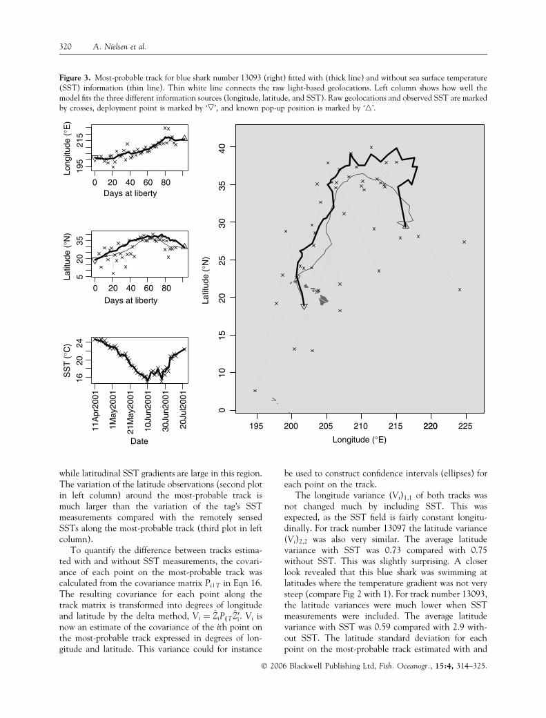
while latitudinal SST gradients are large in this region.The variation of the latitude observations (second plotin left column) around the most-probable track ismuch larger than the variation of the tag’s SSTmeasurements compared with the remotely sensedSSTs along the most-probable track (third plot in leftcolumn).

To quantify the difference between tracks estima-ted with and without SST measurements, the covari-ance of each point on the most-probable track wascalculated from the covariance matrix Pi|T in Eqn 16.The resulting covariance for each point along thetrack matrix is transformed into degrees of longitudeand latitude by the delta method, Vi ¼ ZiPijTZ0

i . Vi isnow an estimate of the covariance of the ith point onthe most-probable track expressed in degrees of lon-gitude and latitude. This variance could for instance

be used to construct confidence intervals (ellipses) foreach point on the track.

The longitude variance (Vi)1,1 of both tracks wasnot changed much by including SST. This wasexpected, as the SST field is fairly constant longitu-dinally. For track number 13097 the latitude variance(Vi)2,2 was also very similar. The average latitudevariance with SST was 0.73 compared with 0.75without SST. This was slightly surprising. A closerlook revealed that this blue shark was swimming atlatitudes where the temperature gradient was not verysteep (compare Fig 2 with 1). For track number 13093,the latitude variances were much lower when SSTmeasurements were included. The average latitudevariance with SST was 0.59 compared with 2.9 with-out SST. The latitude standard deviation for eachpoint on the most-probable track estimated with and

SS

T (

°C)

1620

24

11A

pr20

01

1May

2001

21M

ay20

01

10Ju

n200

1

30Ju

n200

1

20Ju

l200

1

Date

0 20 40 60 80

Days at liberty

520

35

Latit

ude

(°N

)

195

215

0 20 40 60 80Days at liberty

Long

itude

(°E

)

220195 200 205 210 215 220 225

Longitude (°E)

Latit

ude

(°N

)

3540

1520

100

2530

Figure 3. Most-probable track for blue shark number 13093 (right) fitted with (thick line) and without sea surface temperature(SST) information (thin line). Thin white line connects the raw light-based geolocations. Left column shows how well themodel fits the three different information sources (longitude, latitude, and SST). Raw geolocations and observed SST are markedby crosses, deployment point is marked by ‘,’, and known pop-up position is marked by ‘n’.



without SST measurements (Fig. 4) illustrates thedifference. The latitude standard error of the purelylight-based method is between 1.5� and 2�, meaningthat a 95% confidence interval could span up to 8�.

The standard error of the method including SST isbetween 0.4 and 1.5, and about half of the time around0.5, which corresponds to a 95% confidence intervalspanning only 2�. The average longitude variance was2.3 for track number 13093 and 0.54 for track number13097, both estimated in the model with SST.

The double-tagging buoy experiment was not de-signed to evaluate the method of incorporating SST,but to investigate the error structure of light-basedgeolocations. Unfortunately the light-based latitudeinformation from these specific tags produced esti-mates with huge geolocation errors (Figs 5 and 6).With measurement errors of up to 50� latitude, thisinformation is practically useless. However, the dou-ble-tagging buoy experiment offers a unique oppor-tunity to test the SST method in the absence ofconsistent latitude information on a moving tag.

The first double-tagging buoy experiment (Fig. 5)showed that the SST-enhanced method is able toestimate the actual track of the drifter buoy. Theestimated longitude coordinates from the most-prob-able track match the GPS-determined longitude very

0 20 40 60 80

0.0

0.5

1.0

1.5

2.0

Days at liberty

SD

(m

ost p

roba

ble

latit

ude)

Figure 4. Estimated standard deviation for the latitudecomponent of the most-probable track 13093 estimated with(lower thick line) and without sea surface temperatureinformation (upper thin line).

Long

itude

(°E

)

Days at liberty0 50 100 150 200 250

196

199

Latit

ude

(°N

)

Days at liberty0 50 100 150 200 250

−50

50

SS

T (

°C)

2428

10S

ep20

02

30O

ct20

02

19D

ec20

02

7Feb

2003

29M

ar20

03

18M

ay20

03

Date

Days at liberty0 50 100 150 200 250

196

199

Long

itude

(°E

)

Days at liberty0 50 100 150 200 250

Latit

ude

(°N

)

1821

24

SS

T (

°C)

2426

10S

ep20

02

30O

ct20

02

19D

ec20

02

7Feb

2003

29M

ar20

03

18M

ay20

03

Date

Figure 5. Most-probable track for drifter buoy 21760 (solid line) compared with the raw observations (crosses left plot), and tothe true positions from global positioning system measurements (dashed lines right plot). The shaded area indicates a time periodwhen the buoy was beached on an island.



closely, as expected (the root mean squared, or RMS,difference ¼ 0.31�) and are slightly better than theraw longitude (RMS difference ¼ 0.36�). The latitudecoordinates are also close to the GPS-determinedlatitude (RMS difference ¼ 0.99�), which is moreremarkable, as the raw latitude was not very helpful(RMS ¼ 29.23�). The most-probable latitude track isderived almost solely from SST information. The buoybeached itself for a period of 3 weeks and then wentback into the water (Fig. 5). The buoy kept trans-mitting and recording, and the reconstructed trackseems unaffected by stranding.

The second double-tagging buoy experiment(Fig. 6) is more problematic to evaluate, as the buoywas caught on a reef about half of the time. The most-probable longitude track agrees well with the GPSinformation (RMS difference ¼ 0.15) and is betterthan the raw longitude estimates (RMS difference ¼0.32). Raw latitude measurements had errors up to 60�(RMS difference ¼ 36.17) compared with the actualtrack. The most-probable latitude track is off by only

1� or 2� from the actual track and had smaller RMSdifferences (1.00). The buoy entered Maro Reef after120 days at liberty and remained within the reefcomplex for the last 4 months (Fig. 6). The PSATfunctioned normally during this period recording dataand transmitting on schedule.

To illustrate the sensitivity of the degree ofsmoothing to the SST temperature field, three dif-ferent degrees of smoothing were tested on the fourtracks. Normal (5% nearest neighbor fraction), twiceas coarse (10%), and twice as fine (2.5%). Here finerefers to less smoothing, which is closer to the ob-served SST field. This sensitivity analysis showedonly minor differences between the reconstructedtracks (Fig. 7). In fact, most of the tracks wereidentical. In one case, the very finest smoothingseemed to give a more variable track in a fewpoints.

The degree of smoothing used in the track analysiswas chosen simply by looking at the smoothed fieldscompared with the observed fields. A more objective

Long

itude

(°E

)

Days at liberty

0 50 100 150 200 250

185

188

Long

itude

(°E

)

Days at liberty

0 50 100 150 200 250

185

188

Days at liberty

0 50 100 150 200 250

Latit

ude

(°N

)

−60

060

Days at liberty

0 50 100 150 200 250

Latit

ude

(°N

)

2325

27

SS

T (

°C)

1824

17S

ep20

02

6Nov

2002

26D

ec20

02

14F

eb20

03

5Apr

2003

25M

ay20

03

Date

SS

T (

°C)

2225

28

17S

ep20

02

6Nov

2002

26D

ec20

02

14F

eb20

03

5Apr

2003

25M

ay20

03

Date

Figure 6. Most-probable track for drifter buoy 21765 (solid line) compared with the raw observations (crosses left plot), and tothe true positions from GPS measurements (dashed lines right plot). The shaded area indicates a time period when the buoy wascaught on a reef.



and automatic approach would be to select the degreeof smoothing based on a cross-validation scheme(Efron and Tibshirani, 1993).

DISCUSSION

Geolocation based on indirect measurements is un-likely to ever achieve the precision of GPS methods,but combining several indirect measurements in acoherent manner is the best solution possible. Thelatitude variance estimates, (Vi)2,2, are substantiallylower that those anticipated by Smith and Goodman(1986) and approach the theoretical limit discussed byMetcalfe (2001).

The general approach of matching individualmeasurements to a corresponding externally deter-mined field, within the milieu of the Kalman filter, can

potentially be used to further improve (or replace)light-based geolocation by including more measurableor detectable environmental variables. For instancesalinity, geomagnetism, chemical tracers, or waterdepth for demersal species (Hunter et al., 2003). Thepresent paper demonstrates the use of supplementaryfields by illustrating how the inclusion of SST meas-urements is able to reduce the geolocation error sub-stantially (Fig. 4), and even reconstruct a track wherethe light-based latitude measurements were practicallyuseless (Fig. 5). Reduction in geolocation error isgreatest in the directions and areas where the gradientof the ancillary field is steepest. In the case of SST, theSST field in the study area had steepest gradients inthe latitude direction, which is also the directionwhere light-based geolocation is poorest. When con-sidering to include additional variables to improve

0 20 60 100

185

190

195

200

205

210

215

220

20

25

30

35

40

0 40 80 120 0 50 150 250 0 50 150 250

11A

pr20

01

1May

2001

21M

ay20

01

10Ju

n200

1

30Ju

n200

1

20Ju

l200

1

2Apr

2001

22A

pr20

0112

May

2001

1Jun

2001

21Ju

n200

111

Jul2

001

31Ju

l200

120

Aug

2001

10S

ep20

02

30O

ct20

02

19D

ec20

02

7Feb

2003

29M

ar20

03

18M

ay20

03

10S

ep20

02

30O

ct20

02

19D

ec20

02

7Feb

2003

29M

ar20

03

18M

ay20

03

Date

Days at liberty

Latit

ude

(°N

) Lo

ngitu

de (

°E)

13093 13097 21760 21765

Figure 7. Most-probable longitude (top row) and latitude (bottom row) of the four estimated tracks with three levels ofsmoothing of the sea surface temperature (SST) field: normal (dashed line), twice as coarse (solid line), and twice as fine (dottedline). Fine-scale SST fields were applied to tracks 13093 and 13097. Mesoscale data were applied to tracks 21760 and 21765.



geolocation, it should be a concern whether or notthat information is really already implicitly represen-ted. For instance, if the SST and salinity fields areproportional in the study area, it would not contributemuch to include them both. The state space Kalmanfilter approach (Sibert et al., 2003) is an importantpart of the presented method. It ensures that thematching between tag observations and the underlyingfield is made locally. The field can potentially havemany areas where the value matches the tag observedvalue, and the Kalman filter provides an objectivemethod to select the value that is most consistent withall observations.

Drifter buoys are not the perfect tools for evaluatinghow well this method works on live animals, as theirbehavior is somewhat different. Free-ranging largepelagic fish make vertical excursions in the watercolumn and do not run aground. These abnormalperiods could have influenced the SST measurements.The 3-week beaching seems not to have influencedthe measurements or the reconstructed track. The4 months at a fixed position in the shallow waters of areef might have given slightly higher SST readingsthan if a tagged individual was swimming freely in thesurrounding waters. This may account for the moresoutherly estimated track. Despite these difficulties thedrifter buoy experiments demonstrate that SST isuseful in estimating latitude, even when the light-based latitude is practically useless.

The inclusion of ocean temperature in the Kalmanfilter estimation process could result in more accurategeolocations for several pelagic species. Light-basedgeolocations are problematic for species with largediurnal vertical migrations (e.g. swordfish, bigeyetuna and thresher sharks). These species descendbefore dawn to occupy mesopelagic depths during theday and ascend after dusk to occupy near-surfacedepths at night. Latitude estimates are often inac-curate because of dim ambient light at mesopelagicdepths and extensive vertical movements at the timeof dawn and dusk (Musyl et al., 2001). However,these species often occupy the mixed layer during thenight and SST information could improve the geo-locations. Takahashi et al. (2003) used a searchingalgorithm to match tag temperatures at 0, 80 and160 m to ocean temperatures at a monthly 2� lati-tude and 5� longitude scale to estimate latitudes froman archival tag recovered from a swordfish. A similarapproach could be envisaged in a Kalman filter pro-cess whereby tag temperatures at several depths couldbe linked with observed temperature-at-depth data orOceanic General Circulation Model (OGCM) modeloutput.

A simple sensitivity analysis was conducted toillustrate the effect of smoothing the SST temperaturefield. While current results indicate only minor differ-ences when using three different degrees of smoothing,further work is required to investigate the spatial aswell as temporal effects of scale and smoothing. Theappropriate scale of SST data and smoothing willdepend on several factors such as the ocean dynamicsin the study area and data quality because of cloudcover. Scale and smoothing considerations would bedifferent for an analysis of a western boundary current(Kuroshio, Gulf Stream) region compared with a lessstratified mid-ocean gyre. The abundance of cloudsmay dictate the scale and smoothing required as theKalman filter requires that all points be included inthe study area and smoothing was necessary to removeSST pixels with no data (excessive cloud cover),especially in the fine-scale (9 km) data.

Use of the average of the water temperature meas-urements collected from the tag at depths <15 m is anarbitrary choice. Using for instance the median or themode might work equally well (or better) within theframework of the outlined method. Similarly, othersources and scales of SST fields should be considered.

The application of SST to estimation of positionsfrom archival tag data inevitably requires some arbi-trary decisions: a specific SST product, scale, andresolution must be selected; a means to estimate SSTfrom data recorded by the tag must be devised; a cri-terion to determine what constitutes a match betweenenvironmental and tag SST estimates must be speci-fied. Modifications to the Kalman filter model des-cribed here eliminate the third decision by includingthe SST variance in the likelihood function (Eqn 14)in a statistically consistent way with other sources ofvariance. Furthermore, smoothing the SST surface andthe use of averaging to compute the tag SST mitigatethe consequences of the first two decisions. Othertemperature correction methods assume that the light-based longitude estimates are either error free or haveerrors that can be reduced to near zero by removal ofoutliers. The Kalman filter makes no such assumptionsand uses all of the data. In principal, inclusion of SSTalso enables correction of longitude errors where trackscross regions with large longitudinal SST gradients.

ACKNOWLEDGEMENTS

The research was supported by the SLIP researchschool under the Danish Network for Fisheriesand Aquaculture Research (http://www.fishnet.dk)financed by the Danish Ministry for Food, Agricul-ture and Fisheries and the Danish Agricultural and



Veterinary Research Council. The work described inthis paper was partly sponsored by the University ofHawaii Pelagic Fisheries Research Program undercooperative agreement number NA17RJ1230 from theNational Oceanic and Atmospheric Administration.We thank Kevin Wong, NOAA/PIFSC and PhilWhite, crew, and officers of the NOAA research shipTownsend Cromwell for their outstanding help indeploying the drifter buoys and PSAT tags. We thankthe NOAA CoastWatch – Central Pacific Node forproviding SST data. Finally we acknowledge StevenTeo for comments and suggestions to a previous versionof this paper, which greatly improved the final result.

REFERENCES

Arnold, G. and Dewar, H. (2001) Electronic tags in marinefisheries research: a 30-year perspective. In: Electronic Taggingand Tracking in Marine Fisheries Reviews: Methods and Tech-nologies in Fish Biology and Fisheries. J.R. Sibert & J.L. Nielsen(eds) Dordrecht: Kluwer Academic Press, pp. 7–64.

Efron, B. and Tibshirani, R.J. (1993) An Introduction to theBootstrap. London: Chapman & Hall.

Gunn, J. and Block, B. (2001) Advances in acoustic, archival,and satellite tagging of tunas. In: Tuna Physiology, Ecology,and Evolution. B.A. Block & E.D. Stevens (eds) New York:Academic Press, pp. 167–224.

Gunn, J., Polachek, T., Davis, T., Sherlock, M. and Betlehem, A.(1994) The development and use of archival tags for study-ing the migration, behaviour and physiology of bluefin tuna,with an assessment of the potential for transfer of the tech-nology for groundfish research. ICES C.M. Mini 21:1–23.

Harvey, A.C. (1990) Forecasting, Structural Time Series Modelsand the Kalman Filter. Cambridge: Cambridge UniversityPress.

Hill, R. (1994) Theory of geolocation by light levels. In: Ele-phant Seals: Population Ecology, Behaviour, and Physiology.B.J., LeBoeuf & R.M., Laws (eds) Berkeley, CA: Universityof California Press, pp. 227–236.

Hill, R.D. and Braun, M.J. (2001) Geolocation by light level –the next step: latitude. In: Electronic Tagging and Tracking inMarine Fisheries. J.R. Sibert & J. Nielsen (eds) Dordrecht:Kluwer Academic Publishers, pp. 315–330.

Hunter, E., Aldridge, J.N., Metcalfe, J.D. and Arnold, G.P.(2003) Geolocation of free-ranging fish on the Europeancontinental shelf as determined from environmental varia-bles: I. Tidal location method. Mar. Biol. 142:601–609.

Inagake, D., Yanada, H., Segawa, K., Okazaki, M., Nitta, A. andItoh, T. (2001) Migration of young Bluefin Tuna, Thunnusorientalis Temminck et Schlegal, through archival taggingexperiments and its relation with oceanographic conditionsin the western North Pacific. Bull. Nat. Res. Inst. Far SeasFish. 38:53–81.

Jonsen, I.D., Myers, R.A. and Flemming, J.M. (2003) Meta-analysis of animal movement using state-space models.Ecology 84:3055–3063.

Kalman, R.E. (1960) A new approach to linear filtering andprediction problems. Trans. ASME J. Basic Eng. 82:35–45.

Loader, C. (1999) Local Regression and Likelihood. New York:Springer.

Metcalfe, J.D. (2001) Summary report of a workshop on daylightmeasurements for geolocation in animal telemetry. In:Electronic Tagging and Tracking In Marine Fisheries Reviews:Methods and Technologies in Fish Biology and Fisheries. J. Sibert& J. Nielsen (eds) Dordrecht: Kluwer Academic Press, pp.443–456.

Musyl, M.K., Brill, R.W., Curran, D.S. et al. (2001) Ability ofarchival tags to provide estimates of geographical positionbased on light intensity. In: Electronic Tagging and Tracking inMarine Fisheries Reviews: Methods and Technologies in FishBiology and Fisheries. J.R. Sibert & J.L. Nielsen (eds) Dor-drecht: Kluwer Academic Press, pp. 343–368.

Musyl, M.K., Brill, R.W., Boggs, C.H., Curran, D.S., Kazama,T.K. and Seki, M.P. (2003) Vertical movements of bigeyetuna (Thunnus obesus) associated with islands, buoys, andseamounts near the main Hawaiian Islands from archivaltagging data. Fish. Oceanogr. 12:152–169.

Nielsen, A. and Sibert, J. (2005) KFSST: an R-package toefficiently estimate the most probable track from light-basedlongitude, latitude and SST. Available at http://www.soest.hawaii.edu/tag-data/tracking/kfsst.

Reynolds, R.W. and Smith, T.M. (1994) Improved global seasurface temperature analyses using optimal interpolation.J. Clim. 7:929–948.

Sibert, J., Musyl, M.K. and Brill, R.W. (2003) Horizontalmovements of bigeye tuna (Thunnus obesus) near Hawaiidetermined by Kalman filter analysis of archival tagging data.Fish. Oceanogr. 12:141–151.

Smith, P. and Goodman, D. (1986) Determining Fish Movementfrom an ‘Archival’ Tag: Precision of Geographical PositionsMade from a Time Series of Swimming Temperature and Depth.NOAA Technical Memorandum, NOAA-TM-NMFS-SWFC-60, 13 pp.

Takahashi, M., Okamura, H., Yokawa, K. and Okazaki, M.(2003) Swimming behaviour and migration of a swordfishrecorded by an archival tag. Mar. Freshw. Res. 54:527–553.

Teo, S.L.H., Boustany, A., Blackwell, S., Walli, A., Weng, K.C.and Block, B.A. (2004) Validation of geolocation estimatesbased on light level and sea surface temperature from elec-tronic tags. Mar. Ecol. Prog. Ser. 283:81–98.

Vazquez, J., Perry, K. and Kilpatrick, K. (1998) NOAA/NASAAVHRR Oceans Pathfinder Sea Surface Temperature Data SetUser’s Reference Manual, Version 4.0. 10 April 1998. Pasa-dena, CA: Jet Propulsion Laboratory. JPL PublicationD-14070.

Wilson, R.P., Ducamp, J.-J., Rees, W.G., Culik, B.M. andNeikamp, K. (1992) Estimation of location: global coverageusing light intensity. In: Wildlife Telemetry: Remote Monitor-ing and Tracking of Animals. I.G. Priede & S.M. Swift (eds).New York: Ellis Horwood, pp. 131–134.

Wilson, S.G., Lutcavage, M.E., Brill, R.W., Genovese, M.P.,Cooper, A.B. and Everly, A.W. (2005) Movements ofbluefin tuna (Thunnus thynnus) in the northwestern AtlanticOcean recorded by pop-up satellite archival tags. Mar. Biol.146:409–423.



Improving light-based geolocation by including sea surface temperature

Documents

Transcript of Improving light-based geolocation by including sea surface temperature