Improving landfill monitoring programs with the aid of...
96
Evaluating SWIG using Turbo Codes Master of Science Thesis in Communication Engineering OSKAR ARVIDSSON TJ ¨ ADER and LINH TRAN Department of Signals and Systems CHALMERS UNIVERSITY OF TECHNOLOGY Gothenburg, Sweden 2011 Master’s Thesis EX029/2011
Transcript of Improving landfill monitoring programs with the aid of...

Improving landfill monitoring programswith the aid of geoelectrical - imaging techniquesand geographical information systems Master’s Thesis in the Master Degree Programme, Civil Engineering
KEVIN HINE
Department of Civil and Environmental Engineering Division of GeoEngineering Engineering Geology Research GroupCHALMERS UNIVERSITY OF TECHNOLOGYGöteborg, Sweden 2005Master’s Thesis 2005:22
Evaluating SWIG using Turbo CodesMaster of Science Thesis in Communication Engineering
OSKAR ARVIDSSON TJADER and LINH TRAN
Department of Signals and SystemsCHALMERS UNIVERSITY OF TECHNOLOGYGothenburg, Sweden 2011Master’s Thesis EX029/2011

Evaluating SWIG using Turbo CodesOskar S. V. Arvidsson Tjader and Linh M. Tran
c© Oskar S. V. Arvidsson Tjader and Linh M. Tran, 2011
Technical report no EX029/2011 Department of Signals and SystemsChalmers University of TechnologySE-41296 GothenburgSwedenTelephone +46-(0)31 772 1000
Department of Signals and SystemsGothenburg, Sweden 2011

Abstract
Nowadays many larger companies have built up extensive libraries writtenin the system programming languages C or C++. These languages are ca-pable of a wide variety of operations and have very fast execution timescompared to scripting languages. The down-side is that the user friendli-ness and interactivity can become very low. Simplified Wrapper InterfaceGenerator (SWIG) is a software development tool that integrates C/C++modules with scripting languages to exploit the strengths of each language.The objective of this thesis is to evaluate whether SWIG can be used to wrapthe Ericsson library Baseband Core Library (BCL) so that it can be used ina Python environment. The concept was proven by wrapping a turbo codeclass in the open source library IT++. To do this, two data conversion fileswere created to handle the passing of IT++ data structures between C++and Python.
If the library to be wrapped has few dependencies to other libraries andonly contains standard C++ data types, then wrapping with SWIG is ratherstraight forward. The libraries IT++ and BCL however use IT++ defineddata structures which introduces additional complexity. To decide whetherit is beneficial to wrap modules with converter files and glue code one shouldconsider the amount of time and effort that is required to write the glue codescompared to the amount of usage.

”Experience is what you get when you didn’t get what you wanted”
— Anders Hansson, quoting Randy Pausch, referencing a quote used at Electronic Arts

Contents
1 Introduction 51.1 Background . . . . . . . . . . . . . . . . . . . . . . . . . . . . 51.2 Objective and Approach . . . . . . . . . . . . . . . . . . . . . 6
1.2.1 Scope . . . . . . . . . . . . . . . . . . . . . . . . . . . 7
2 IT++ 82.1 Vector Class . . . . . . . . . . . . . . . . . . . . . . . . . . . . 82.2 Turbo Code Class . . . . . . . . . . . . . . . . . . . . . . . . . 9
3 SWIG 103.1 Comparison of C++ and Python . . . . . . . . . . . . . . . . 11
3.1.1 C++ . . . . . . . . . . . . . . . . . . . . . . . . . . . . 113.1.2 Python . . . . . . . . . . . . . . . . . . . . . . . . . . . 113.1.3 Combining the Languages . . . . . . . . . . . . . . . . 12
3.2 SWIG Structure . . . . . . . . . . . . . . . . . . . . . . . . . . 133.2.1 Interface File . . . . . . . . . . . . . . . . . . . . . . . 133.2.2 SWIG Output . . . . . . . . . . . . . . . . . . . . . . . 14
3.3 Templates . . . . . . . . . . . . . . . . . . . . . . . . . . . . . 163.3.1 Templates in C++ . . . . . . . . . . . . . . . . . . . . 163.3.2 Templates in SWIG . . . . . . . . . . . . . . . . . . . . 17
3.4 Namespaces . . . . . . . . . . . . . . . . . . . . . . . . . . . . 193.5 Type Conversion . . . . . . . . . . . . . . . . . . . . . . . . . 193.6 SWIG Libraries . . . . . . . . . . . . . . . . . . . . . . . . . . 20
3.6.1 std vector.i . . . . . . . . . . . . . . . . . . . . . . . . 203.6.2 std string.i . . . . . . . . . . . . . . . . . . . . . . . . . 21
4 Turbo and Turbo-like Codes 224.1 Discrete-time Equivalent Baseband Model . . . . . . . . . . . 22

CONTENTS 3
4.2 Convolutional Codes . . . . . . . . . . . . . . . . . . . . . . . 234.2.1 Code Weight and Minimum Distance . . . . . . . . . . 274.2.2 Recursive Convolutional Encoders . . . . . . . . . . . . 27
4.3 Maximum Likelihood Sequence Decoding and the Viterbi Al-gorithm . . . . . . . . . . . . . . . . . . . . . . . . . . . . . . 28
4.4 Maximum A-Posteriori Symbol Decoding . . . . . . . . . . . . 294.5 BCJR Algorithm . . . . . . . . . . . . . . . . . . . . . . . . . 29
4.5.1 A Posteriori Information . . . . . . . . . . . . . . . . . 304.5.2 Derivation of α, β, γ . . . . . . . . . . . . . . . . . . . 314.5.3 Decoding . . . . . . . . . . . . . . . . . . . . . . . . . 334.5.4 Outline of the Algorithm . . . . . . . . . . . . . . . . . 34
4.6 Turbo Codes . . . . . . . . . . . . . . . . . . . . . . . . . . . . 344.6.1 Concatenated Codes with Interleaver . . . . . . . . . . 344.6.2 Extrinsic Information . . . . . . . . . . . . . . . . . . . 374.6.3 Iterative Decoding . . . . . . . . . . . . . . . . . . . . 38
5 Implementation and Results 415.1 Wrapping IT++ . . . . . . . . . . . . . . . . . . . . . . . . . 42
5.1.1 Libraries . . . . . . . . . . . . . . . . . . . . . . . . . . 445.2 Wrapping BCL . . . . . . . . . . . . . . . . . . . . . . . . . . 45
6 Discussion and Conclusion 47References . . . . . . . . . . . . . . . . . . . . . . . . . . . . . . . . 50
Acronyms 51
A User’s Guide 53A.1 Setup . . . . . . . . . . . . . . . . . . . . . . . . . . . . . . . . 53A.2 Wrap . . . . . . . . . . . . . . . . . . . . . . . . . . . . . . . . 53
B Code 55B.1 SWIG modules . . . . . . . . . . . . . . . . . . . . . . . . . . 55
B.1.1 demo.cc . . . . . . . . . . . . . . . . . . . . . . . . . . 55B.1.2 demo.h . . . . . . . . . . . . . . . . . . . . . . . . . . . 57B.1.3 demo.i . . . . . . . . . . . . . . . . . . . . . . . . . . . 58B.1.4 setup.py . . . . . . . . . . . . . . . . . . . . . . . . . . 58B.1.5 turbo.py . . . . . . . . . . . . . . . . . . . . . . . . . . 59B.1.6 converters.cc . . . . . . . . . . . . . . . . . . . . . . . . 61

CONTENTS 4
B.1.7 converters.h . . . . . . . . . . . . . . . . . . . . . . . . 64B.1.8 converters.py . . . . . . . . . . . . . . . . . . . . . . . 64B.1.9 com funcs.py . . . . . . . . . . . . . . . . . . . . . . . 65
B.2 Turbo Code . . . . . . . . . . . . . . . . . . . . . . . . . . . . 68B.2.1 turbo.py . . . . . . . . . . . . . . . . . . . . . . . . . . 68B.2.2 com funcs.py . . . . . . . . . . . . . . . . . . . . . . . 73B.2.3 help funcs.py . . . . . . . . . . . . . . . . . . . . . . . 76B.2.4 outer encoder.py . . . . . . . . . . . . . . . . . . . . . 79B.2.5 inner encoder.py . . . . . . . . . . . . . . . . . . . . . 81B.2.6 BCJR outer.py . . . . . . . . . . . . . . . . . . . . . . 84B.2.7 BCJR inner.py . . . . . . . . . . . . . . . . . . . . . . 89

Chapter 1
Introduction
1.1 Background
Nowadays many larger companies have built up extensive libraries to beused for their development needs. At many times these libraries are crucialto achieve results that are of direct relevance for the company. They are oftenwritten in the system programming languages C or C++. These languagesare capable of a wide variety of operations from low-level operations suchas flipping bits and manipulating inputs as well as higher-level operations.This makes them suitable for building up libraries from scratch. C and C++also have very fast execution times which is required for some applications.The down-side to all this is that the user friendliness and interactivity canbecome very low for users of the library. The sheer size and complexity ofthese libraries can make a trivial task complicated. The system programminglanguages are also not suitable when small code changes have to be performedoften. After each change, no matter how small, the code will have to be re-compiled for the changes to come into effect.
Scripting languages on the other hand were not primarily meant for build-ing programs from scratch but rather for plugging together existing programsand functions. For this task they are very flexible. Since scripting languagesuse interpreters and not compilers there is also no lengthy compilation timebetween code changes. They do however have longer execution times becauseof this.
As can be seen, both types of languages have their advantages and hencea way to combine these advantages would be valuable. One way of solving
1.2 Objective and Approach 6
this is by using Simplified Wrapper Interface Generator (SWIG). SWIG is asoftware development tool that generates wrappers for C and C++ modulesso that these can be used by scripting languages.
Baseband Core Library (BCL) is a large library developed by Ericsson,containing functions for simulating baseband communication. It is writtenin C++ and is quite large and complex, around 500,000 lines of code intotal. If this library could be wrapped using SWIG, it would greatly aid inits development and testing.
For Ericsson the desired scripting language to integrate with BCL isPython. Python has a syntax which is similar to MATLAB and supportsobject orientation and advanced data structures which makes it suitable forEricsson’s needs.
1.2 Objective and Approach
The objective of this master thesis work is to evaluate whether SWIG can beused to wrap BCL so that it can be used in a Python environment. A largeand complex library like BCL is however not the ideal starting library towrap with SWIG. The details of BCL are also confidential and hence cannotbe covered in this report. However, BCL uses data structures from the opensource library IT++ developed at Chalmers University of Technology. IT++is a library which contains mathematical, signal processing and communica-tion classes and functions intended to be used for communications relatedsimulations. It is also a library, which compared to BCL, contains fewerdependencies to other libraries. This reduces the complexity of wrappingit considerably. As a proof of concept, the IT++ library will therefore bewrapped. This will show how SWIG can be used to wrap a library that isapplicable to Ericsson’s needs. Given how BCL uses IT++ data structures,successfully wrapping IT++ will also be a step towards wrapping BCL. Tothe best of our knowledge this has not been accomplished before in a waythat allows data to be passed back and forth between Python and IT++using SWIG.
A good choice for showcasing how SWIG can be used by Ericsson is towrap the turbo encoder and decoder in IT++. This is a non-trivial classwhich can be troublesome to implement. It also requires many computationswhich makes it preferable to implement in a language with fast executiontime. On top of this there are few dependencies to other classes which might

1.2 Objective and Approach 7
otherwise cause difficulties. With the Turbo class wrapped, it can be usedinteractively in a Monte Carlo loop in Python. The generation of informa-tion bits, modulation, addition of noise, and other trivial communicationoperations can be done in Python while the actual turbo details are done inthe wrapped IT++ turbo encoder and decoder. Once this configuration isimplemented it will be possible to manipulate the inputs and outputs of theturbo class functions as well as store and plot data using only Python. In thisreport we will showcase this by running the Monte Carlo loop and generatingBit Error Rate (BER) plots for a range of Signal to Noise Ratio (SNR) val-ues. A turbo encoder and decoder will be implemented in Python to test andverify the Monte Carlo loop until the IT++ decoder is successfully wrapped.
In order to do this, however, we need to understand how a turbo decoderworks within a communication system. To be able to combine it with Pythonand give the various functions the correct inputs and outputs an explanationof the theory behind turbo codes is covered.
Once IT++ is successfully wrapped the task of wrapping BCL can bestarted. As in the IT++ case a single class from BCL will be wrapped. Asmentioned before, the details of this class cannot be presented due to Ericssonconfidentiality but the lessons learned will be explained in this report.
1.2.1 Scope
A comparable solution for intregrating IT++ or BCL with a scripting lan-guage is to use MEX to integrate the library with MATLAB. Since Ericssonwas interested in Python such a solution was never considered in any detailand will hence not be covered by this report.
There exists many other programs, such as Pyrex, SIP, and Boost, whichperform similar functions to SWIG. In this master thesis SWIG is covered.The analyzed version of SWIG is 2.0 which is integrated with Python 3.1.1.
Since BCL and IT++ are both based on C++, modules written in thislanguage will be wrapped. Focus is mainly put on wrapping a turbo code.
Chapter 2
IT++
IT++ is an open source C++ library of mathematical, signal processing andcommunication classes and functions [1]. It is mainly used for simulation andresearch in the communications area. The library was originally developedat the former department of Information Theory at Chalmers University ofTechnology in Sweden.
The library contains definitions of classes with associated routines whichmakes it possible to create data structures in C++ in a similar way as inMATLAB or GNU Octave. It covers a wide span of modules in a communica-tion system, from basic components such as vectors, matrices and classes forrandom number generation to more advanced classes for channel modeling,interleaving, encoding, and decoding.
To demonstrate how IT++ can be used we give two short examples inthe following sections.
2.1 Vector Class
IT++ defines a class Vec<Num T> which utilizes the template feature inC++. It makes it possible to create vectors of different types, such as int,double, etc. For example, we can create a vector of type double with thefollowing line
vec my vector ;
As in MATLAB, many operations can be performed on the vector. Forinstance we can create a vector of zeros with length n with
2.2 Turbo Code Class 9
my vector = ze ro s (n ) ;
We can also insert, remove or shift elements in a vector, or concatenateseveral vectors.
IT++ provides an Application Programming Interface (API) that de-scribes all classes and functions. In a similar way matrices can be createdand operations performed according to the API.
2.2 Turbo Code Class
One of the more advanced classes implemented in IT++ is Turbo Codec, theclass that will be wrapped in this thesis. It implements a turbo encoderand decoder which has several parameters such as the choice of decodingmethod, interleaver length, encoder generator vectors, number of iterations,etc. The details of these parameters will be discussed in Chapter 4. Many ofthe functions in Turbo Codec takes different types of Vec<Num T> as input.How these types can be passed from python to C++ are described in section5.1.

Chapter 3
SWIG
SWIG is a software development tool that connects programs written inC/C++ with scripting languages such as Python, Perl, and Tcl. By takingthe declarations in the C/C++ header files it generates a glue code (wrapper)that enables the target languages to call functions within the C/C++ code.Figure 3.1 illustrates the basic idea behind SWIG.
Script language
SWIG wrapper
C/C++ module
Figure 3.1: Basic idea behind SWIG.
For simplicity’s sake, in the following sections the examples are writtenfor C++ only.

3.1 Comparison of C++ and Python 11
3.1 Comparison of C++ and Python
Combining a scripting language, such as Python, with a system programminglanguage like C++ is very powerful since it can exploit the strengths of eachlanguage. In this section the strengths and weaknesses relevant for buildingand using large libraries with these languages will be covered.
3.1.1 C++
C++ is a language intended to function on a mid-level of programming,meaning that it has to be capable of both low- and high-level operations.This results in a very flexible programming language that can interact withhardware with few restrictions but also function on a higher level of abstrac-tion [2]. This allows for almost any complex data structure or algorithm tobe implemented and the flexibility makes it suitable for building a librarysuch as BCL from scratch. The down-side to this is that the code can oftenbecome quite large and complex. Since the library is built from scratch theprogrammer also needs to understand both high- and low-level programming.
C++ is based on static typing which means that the type is checked whenthe code is compiled and not during run-time. This allows the compiler todetect certain type related errors. It also allows the compiler to generatespecialized code. For example, since it already knows the type it can justgenerate type specific instructions without any additional instructions fortype checking. This optimization gives very fast execution times. It doeshowever mean that code cannot be easily re-used. In addition, the codehas to be re-compiled between each change, no matter how insignificant itmay be. For large codes or libraries this can be a considerable delay indevelopment time [3].
3.1.2 Python
Python on the other hand is a scripting language, which has somewhat dif-ferent characteristics than C++. The first, and probably greatest, differenceis that unlike C++ a scripting language assumes that useful components,written in other languages, already exist. In other words it is not designedto build programs from scratch but rather plugging or ”gluing” together ex-isting components. For this reason scripting languages are also referred to as
3.1 Comparison of C++ and Python 12
system integration languages or glue languages. In order to allow this con-nectivity between components, scripting languages are usually typeless. Thismeans that there are no prior restrictions forced upon the data. Any com-ponent or value can thereby be used in any situation. This allows for codeto be re-used for tasks the programmer never intended. This does howeverrequire instructions for type checking. Another major difference comparedto C++ is that Python is not compiled but interpreted, which eliminatescompilation time. The price one pays for these advantages is execution time.This is the result of using interpreters instead of compilers as well as havingthe components designed for ease of use instead of efficient mapping ontounderlying hardware.
Python is a higher level programming language than C++ regarding thenumber of operations a single statement performs on average. Statementsin a scripting language, such as Python, can produce hundreds to thousandsof machine instructions, whereas a typical statement in languages like C++executes five machine instructions on average [4]. The main cause for this isthat the primitive operations in scripting languages are much more powerfulthan in languages like C++ [4].
As a scripting language, Python distinguishes itself in a number of wayswhich is of interest for Ericsson. It has a syntax that can be very similarto MATLAB, which is a language already used at Ericsson. Additionally,Python also allows for more advanced data structures than MATLAB. It alsosupports object orientation which can be useful in numerous applications.Another advantage with Python are the many already existing functionsavailable. Besides the standard libraries there are also many third partymodules.
3.1.3 Combining the Languages
As the two previous sections show there are advantages and disadvantagesof both languages. The purpose of SWIG can hence be seen as combiningthe advantages of both languages. By wrapping C++ libraries to Pythonthe speed and flexibility of C++ can be combined with the interactivity andease of use of Python. In theory, this can be used to reduce the developmenttime.

3.2 SWIG Structure 13
3.2 SWIG Structure
In this section we will go through the structure and components of SWIG.Figure 3.2 illustrates the key components and their inter-dependencies togenerate the final extension module.
interface fileexample.i
setup filesetup.py
Distutils
input
shared library_example.so
generates
SWIG
input
python fileexample.py
generates
import to
wrapperexample_wrap.cxx
generates input
Python
import to
created by user
Figure 3.2: SWIG dependencies.
3.2.1 Interface File
The input to SWIG is a file containing ANSI C/C++ and special SWIGdeclarations. Normally this file is a special SWIG interface file denoted witha .i or .swg suffix. Below follows an example of the most common appearanceof a basic SWIG interface file
%module example%{#inc lude ”example . h”%}// ANSI C/C++ dec l a r a t i o n sint func ( int x , int y ) ;int another func ( int x ) ;. . .

3.2 SWIG Structure 14
The name of the module generated by SWIG is given after the %module
directive. In the %{ ... %} block all header files and declarations that areneeded to make the wrapper code compile should be included. This text isnot parsed or interpreted by SWIG but only copied to the generated wrapperfile. At the end of the file all functions that should be accessible from Pythonshould be declared.
3.2.2 SWIG Output
The output from SWIG consist of two files: a Python source file and a C++source file that contains all the wrapper code that is required to build theextension module.
The command line
swig −c++ −python example . i
will produce a C++ source file example wrap.cxx and a Python source fileexample.py. The name of the wrapper comes from SWIG taking the nameof the interface file and appending wrap to it. To create the final extensionmodule the C++ source file needs to be compiled and linked with the rest ofthe C++ program. The Python source file is the file that will be importedinto Python in order to use the module.
The recommended way to build an extension module for python is to usedistutils. Distutils is a package in Python which provides support for build-ing and installing additional modules into Python installations. It makessure that the extension is built with the correct flags and headers etc. for thePython version that is being used. Distutils compiles the SWIG generatedwrapper code into a shared library (.so-file for Linux and .pyd-file for Win-dows) that is included in the Python source file. The compilation is doneby using a configuration file that describes the related extensions. Such aconfiguration file is conventionally called setup.py but can assume any name.Below follows an example
from d i s t u t i l s . core import setup , Extension
example module = Extension ( ’ example ’ ,s ou r c e s =[ ’ example wrap . cxx ’ ,
’ example . cpp ’ ] ,)

3.2 SWIG Structure 15
setup (name = ’ example ’ ,v e r s i on = ’ 1 .0 ’ ,author = ”Linh and Oskar” ,d e s c r i p t i o n = ””” Simple swig example ””” ,ext modules = [ example module ] ,py modules = [ ”example” ] ,)
The line example module = Extension(...) generates an extension module ob-ject using the source code files example wrap.cxx and example.cpp (the originaltarget source file) and sets the name of the module to example. Extensionmodules to SWIG are normally named by using the same name as the pythonmodule prefixed with an underscore. In this case the name of the librarywould then be example.so for Linux. The command to build the sharedlibrary using the setup file and distutils is
python setup . py bu i l d ex t −−i np l a c e
where
• python - is the version of Python we want to use
• setup.py - is the name of the configuration file
• build ext - tells distutils to build extensions
• −−inplace - tells distutils to put the extension lib in the current direc-tory.
An alternative way to create the extension module is to let distutils handlethe generation of the wrapper code and Python source file. Distutils supportscreation of SWIG extension modules and so by modifying the configurationfile slightly we can generate the extension module by only running the lastdistutils command. The setup.py file would then look like this
from d i s t u t i l s . core import setup , Extension
example module = Extension ( ’ example ’ ,s ou r c e s =[ ’ example . i ’ ,
’ example . cpp ’ ] ,sw ig opt s=[ ’−c++’ ]
)

3.3 Templates 16
setup (name = ’ example ’ ,v e r s i on = ’ 1 .0 ’ ,author = ”Linh and Oskar” ,d e s c r i p t i o n = ””” Simple swig example ””” ,ext modules = [ example module ] ,py modules = [ ”example” ] ,)
A second argument, swig opts, has now been added to the Extension con-structor which specifies the target language for the generated wrapper. Also,instead of giving the wrapper file as source we take the interface file. Thebuild ext command will then run SWIG on the interface file and compile theresulting C++ file into the final extension module [5].
Other necessary arguments to the Extension constructor are
• include dirs — the paths to directories where include files are stored
• library dirs — the paths to directories where libraries are stored
• libraries — names of included libraries.
Due to circular dependency the listed order of the libraries in the setupfile is important. That is, if library B depend on library A, then A should beput before B in the list. Also, note that all libraries included in the setup fileshould be built with the same compiler version as the one used for SWIG.
3.3 Templates
Templates can be of use in a wide variety of applications. In signal processingtemplates can be used for representing different bit widths or hard or softinformation. One can for instance use a float or double that can contain 4and 8 bytes of data respectively to represent the bit widths.
Templates allows one to create special functions or classes that can op-erate with generic types. These functions and classes can be adapted tomore than one type without rewriting the entire code for each type by usingtemplate parameters.
3.3.1 Templates in C++
The syntax for declaring a function template with template parameters inC++ is

3.3 Templates 17
template <class i d e n t i f i e r > f u n c t i o n d e c l a r a t i o n ;
For example this could look like
template <class T> void f unc t i on (T x ) ;
where T could be an int, double, float, etc. To call this function we canwrite
int x ;funct ion<int> ( x ) ;
3.3.2 Templates in SWIG
Compilers do not treat templates as normal functions or classes. Templatesare compiled on demand, which means that they are not compiled untilan instantiation with specific template arguments is required. When it isrequired the compiler generates a function specifically for the given arguments[2]. Because of this characteristic, information about a specific templateinstantiation needs to be provided to SWIG in order to wrap a template.Let us illustrate this with the following example code
// Header f i l e : s t a c k . h
template <class T>class MyStack {
MyStack ( ) ;void push (T i ) ;T pop ( ) ;int top ;T s t [ 1 0 0 ] ;
} ;
// C++ f i l e : s t a c k . cc
#inc lude ” stack . h”
template <class T>MyStack<T> : :MyStack ( ){
top = −1;}

3.3 Templates 18
template <class T>void MyStack<T> : : push (T i ){
s t [++top ] = i ;}
template <class T>T MyStack<T> : : pop ( ){
return s t [ top−−];}
These template declarations alone will be ignored by SWIG since it cannotgenerate any code until a definition of the type T is given. One way to createwrappers for templates is to use the %template directive as
%template ( in tStack ) MyStack<int >;%template ( doubleStack ) MyStack<double>;
where the argument to %template() is the name of the instantiation in thetarget language.
Since templates are compiled when required, the declaration and defini-tion of a template function/class must be in the same file. Therefore, if wehave a separate header file for the interface and one with the implementation(definition), then these must be included in the file that uses the template.This means that in SWIG we need to include both the .h-file and .cpp-filein the interface file where the %template directive is used. The interface filewould then have the following look
%module s tack%{
#inc lude ” stack . h”#inc lude ” stack . cpp”
%}
%inc lude ” stack . h”%inc lude ” stack . cc ”%template ( in tStack ) MyStack<int >;
With these directives included in the interface file we can create an instanti-ation of MyStack<int>::MyStack() directly from python as
3.4 Namespaces 19
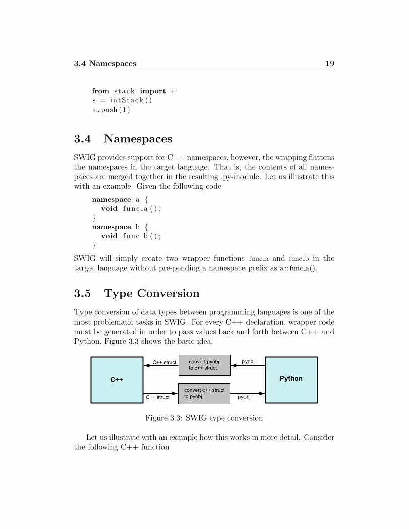
from s tack import ∗s = intStack ( )s . push (1 )
3.4 Namespaces
SWIG provides support for C++ namespaces, however, the wrapping flattensthe namespaces in the target language. That is, the contents of all names-paces are merged together in the resulting .py-module. Let us illustrate thiswith an example. Given the following code
namespace a {void func a ( ) ;
}namespace b {
void func b ( ) ;}
SWIG will simply create two wrapper functions func a and func b in thetarget language without pre-pending a namespace prefix as a :: func a().
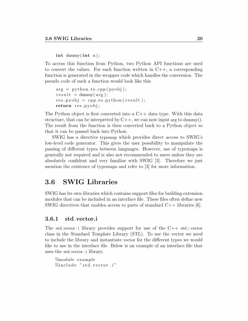
3.5 Type Conversion
Type conversion of data types between programming languages is one of themost problematic tasks in SWIG. For every C++ declaration, wrapper codemust be generated in order to pass values back and forth between C++ andPython, Figure 3.3 shows the basic idea.
Python
convert pyobj to c++ struct
convert c++ struct to pyobj
C++
pyobj
C++ struct pyobj
C++ struct
Figure 3.3: SWIG type conversion
Let us illustrate with an example how this works in more detail. Considerthe following C++ function
3.6 SWIG Libraries 20
int dummy( int n ) ;
To access this function from Python, two Python API functions are usedto convert the values. For each function written in C++, a correspondingfunction is generated in the wrapper code which handles the conversion. Thepseudo code of such a function would look like this
arg = python to cpp ( pyobj ) ;r e s u l t = dummy( arg ) ;r e s pyob j = cpp to python ( r e s u l t ) ;return r e s pyob j ;
The Python object is first converted into a C++ data type. With this datastructure, that can be interpreted by C++, we can now input arg to dummy().The result from the function is then converted back to a Python object sothat it can be passed back into Python.
SWIG has a directive typemap which provides direct access to SWIG’slow-level code generator. This gives the user possibility to manipulate thepassing of different types between languages. However, use of typemaps isgenerally not required and is also not recommended to users unless they areabsolutely confident and very familiar with SWIG [3]. Therefore we justmention the existence of typemaps and refer to [3] for more information.
3.6 SWIG Libraries
SWIG has its own libraries which contains support files for building extensionmodules that can be included in an interface file. These files often define newSWIG directives that enables access to parts of standard C++ libraries [6].
3.6.1 std vector.i
The std vector . i library provides support for use of the C++ std :: vector
class in the Standard Template Library (STL). To use the vector we needto include the library and instantiate vector for the different types we wouldlike to use in the interface file. Below is an example of an interface file thatuses the std vector . i library.
%module example%inc lude ” s t d v e c t o r . i ”
3.6 SWIG Libraries 21
namespace std {%template ( v e c t o r i ) vector<int >;%template ( v e c t o r s ) vector<s t r i ng >;
} ;
Here we have made two instantiations of the vector class. One is of the typeint and the other of type string . Assume we have a C++ function that lookslike the following
void p r i n t v e c t o r ( vector<int> v ) {for ( int i =0; i<v . s i z e ( ) ; i++) {
cout << v [ i ] << endl ;}
}
we can then create a vectori object in Python, fill it with data and input itto print vector . When a vector<int> is returned from C++ to Python it isinterpreted as the Python data structure list .
3.6.2 std string.i
Another library is std string . i which enables passing of the object string inSWIG. To use the library it should be included in the interface file with the%include directive similar to the example in section 3.6.1.

Chapter 4
Turbo and Turbo-like Codes
Turbo codes revolutionized the coding community by achieving performanceclose to the Shannon limit. Today they are used in many communicationsystems. In this chapter we will explain the relevant theory for understandingthe basics of turbo and turbo-like codes.
4.1 Discrete-time Equivalent Baseband Model
Consider the transmission system in Figure 4.1. This is the transmission sys-tem model that subsequent sections will be based upon. It is a discrete-timeequivalent baseband model similar to the one Schlegel and Perez introducein [7]. A way of obtaining this model is through matched filtering.
Convolutional Encoder
AWGN DecoderModulationu c x r û
Figure 4.1: Reference Transmission System
The input to the system is the binary information sequence uK1 of length
K. Each bit, uk, is assumed to be independently drawn from a uniformdistribution {0, 1}. It can be interpreted as data subject to perfect sourcecompression, i.e., no redundancy. This information sequence is encoded bya convolutional encoder, generating the code sequence
cK1 = (c1, c2, . . . , cK) (4.1)

4.2 Convolutional Codes 23
where the length of each ck is n0. The code sequence is modulated to formthe symbol sequence, xS
1 where each symbol, xs, belongs to some finite dis-crete alphabet and the length of the sequence, S, depends on the chosenmodulation. Any modulation could be used but for simplicity we will in thisreport limit us to only using Binary Phase Shift Keying (BPSK). This resultsin the modulated sequence, xK
1 , and each symbol, xk, taking on the values{−√Es,+
√Es
}.
The output sequence, xK1 , is the input to the Additive White Gaussian
Noise (AWGN) channel. The white gaussian noise vector nK1 is added to the
signal forming the received sequence, rK1 as
rK1 = xK1 + nK
1 (4.2)
where E {nk} = 0 and E {nknl} = N0/2δkl where δkl is the Kroneckerdelta.
The decoder’s task is based on decoding the received sequence, rKk out-putting the best possible decision, uK
1 , of the input information sequence.
4.2 Convolutional Codes
Binary convolutional encoders are finite-memory systems which for every k0information bits inserted generate n0 binary output bits. Hence the coderate, Rc, is defined as
Rc = k0/n0. (4.3)
The encoder is composed of N shift registers containing k0 bits, giving atotal of Nk0 stages inside the encoder, see Figure 4.2. The parameter N iscalled the convolutional code’s constraint length. At each time instance t,the block of bits inside each shift register is shifted to the next one to theright and a new block of k0 information bits is inserted into the first, andnow empty, input shift register. The bit values of these positions are thenused by n0 modulo-2 adders to generate n0 code bits that are fed to theoutput register. It can be concluded that such encoders’ output code bitsare not only dependent on the current input bits but on all M = k0(N − 1)previous ones [8]. These bits correspond to the state of the encoder and willbe defined as
Sk =(s(1)k , s
(2)k , · · · , s(M)
k
)(4.4)
4.2 Convolutional Codes 24
1 2 k0. . . 1 2 k0
. . . 1 2 k0. . . 1 2 k0
. . .
1 2 . n0. .
. . .
u
k0
information bits
c n0
coded bits
} } }1 2 N. . . . .
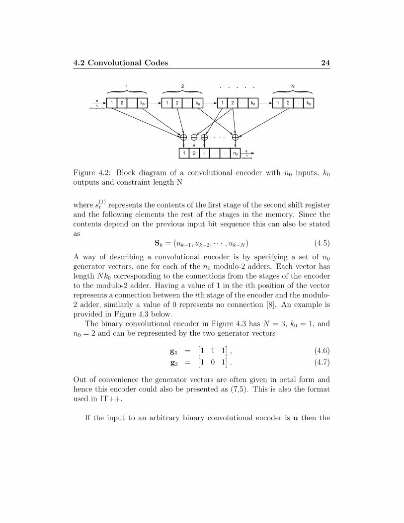
Figure 4.2: Block diagram of a convolutional encoder with n0 inputs, k0outputs and constraint length N
where s(1)t represents the contents of the first stage of the second shift register
and the following elements the rest of the stages in the memory. Since thecontents depend on the previous input bit sequence this can also be statedas
Sk = (uk−1, uk−2, · · · , uk−N) (4.5)
A way of describing a convolutional encoder is by specifying a set of n0
generator vectors, one for each of the n0 modulo-2 adders. Each vector haslength Nk0 corresponding to the connections from the stages of the encoderto the modulo-2 adder. Having a value of 1 in the ith position of the vectorrepresents a connection between the ith stage of the encoder and the modulo-2 adder, similarly a value of 0 represents no connection [8]. An example isprovided in Figure 4.3 below.
The binary convolutional encoder in Figure 4.3 has N = 3, k0 = 1, andn0 = 2 and can be represented by the two generator vectors
g1 =[1 1 1
], (4.6)
g2 =[1 0 1
]. (4.7)
Out of convenience the generator vectors are often given in octal form andhence this encoder could also be presented as (7,5). This is also the formatused in IT++.
If the input to an arbitrary binary convolutional encoder is u then the

4.2 Convolutional Codes 25
uk uk-1 uk-2uk
ck1
ck2
Figure 4.3: [7,5] encoder
output sequence is given by:
c(1) = u ∗ g1 (4.8)
c(2) = u ∗ g2 (4.9)...
c(n0) = u ∗ gn0 (4.10)
where ∗ represents convolution using binary arithmetic. The output codesequence c is then formed in the following manner
cK1 =
(c(1)1 , c
(2)1 , · · · , c(n0)
1 , c(1)2 , c
(2)2 , · · · , c(n0)
2 , · · · , c(1)K , c(2)K , · · · , c(n0)
K
). (4.11)
For our (7,5) encoder the output sequence will be formed as
c(1)k = uk + uk−1 + uk−2 (4.12)
c(2)k = uk + uk−2 (4.13)
ck = (c(1)k , c
(2)k ) (4.14)
It is common that the D-transform is used to explain the operation of aconvolutional encoder. This transform is equivalent to the z-transform exceptthat the operator is D = z−1. If the discrete time input to an arbitrary binaryconvolutional encoder is uk then let the corresponding D-transform be
u(D) =∑k
ukDk (4.15)

4.2 Convolutional Codes 26
The generator vectors can also be represented using the D-transform. Forthe (7,5) example the generators would be expressed as
g1(D) = 1 +D +D2
g2(D) = 1 +D2 (4.16)
It is now possible to express the encoder operation for this example as afunction of the input and generator vectors as
c(1)(D) = u(D)g1(D) (4.17)
c(2)(D) = u(D)g2(D). (4.18)
(4.19)
An alternative description of the binary convolutional encoder is the trel-lis diagram which connects different states over subsequent time steps. Anexample of such a trellis diagram is shown in Figure 4.4 which illustrates thebefore-mentioned (7,5) encoder. The nodes along the same vertical axis rep-resent the various states at that discrete time k. In general there will be 2M
such states. Each of these states would have 2k0 branches entering it and 2k0
branches leaving it, one for each possible input segment. The branch fromone state to another represents new inputs affecting the state of the encoderand generating the corresponding code bits. The code bits generated by eachbranch between two states given an input are written alongside these edgesin the format input/code bits in 4.4. The branches between different stateswill generate a path through the trellis. This path is unique for a given inputsequence and starting state.
State
00
01
10
11
m
0
1
2
3
k = 0 1 2 3 4 5 6
0/00 0/00 0/00 0/00 0/00 0/00
1/11 1/11 1/11 1/11
0/11 0/11 0/11 0/11
1/00 1/00
0/10 0/10 0/10 0/10
1/01 1/01 1/01
0/01 0/01 0/01
1/10 1/10
Figure 4.4: Trellis for (7,5) code
Customarily the code sequence is started and terminated in the S = 0state of the trellis.

4.2 Convolutional Codes 27
4.2.1 Code Weight and Minimum Distance
The weight of a codeword, c ∈ C, is the number of nonzero componentsof that codeword and is expressed as w(c). For linear codes the distancebetween two codewords can be written as d(c1, c2) = w(c1 − c2). A usefulmetric for evaluating codes is the minimum distance, dmin, which is the theminimum of all possible distances between codewords and is expressed as
dmin = minc1,c2∈Cc1 6=c2
d(c1, c2) (4.20)
4.2.2 Recursive Convolutional Encoders
A systematic encoder is an encoder where the input sequence is a directpart of the output sequence. It can be proven that systematic convolutionalencoding, in general, will give lower minimum distances than nonsystematicencoders [8]. Using recursion, it is however possible to construct systematicencoders from any nonsystematic encoder of rate 1/n0 while maintaining thesame minimum distance as the nonsystematic encoder. As can be seen in(4.17), in order to have the input sequence included directly in the output,one of the generator polynomials has to be equal to one. To achieve this, letus divide each encoder output by g1(D), which results in
c(1)(D) = u(D)g1(D)
g1(D)= u(D)
c(2)(D) = u(D)g2(D)
g1(D)...
c(n0)(D) = u(D)gn0(D)
gn0(D). (4.21)
This corresponds to a convolutional encoder with feedback [8]. It is realizedwith shift registers and feedback. Such codes are commonly referred to asRecursive Convolution Codes (RCC). An example of how this can be imple-mented for the (7,5) encoder is shown in (4.21). It can be proven that suchan encoder is equivalent to the original non-recursive non-systematic encodersince both will generate the same set of codewords, albeit for different inputsequences [9].
4.3 Maximum Likelihood Sequence Decoding and the ViterbiAlgorithm 28
uk-1 uk-2
ck1
ck2
ukuk
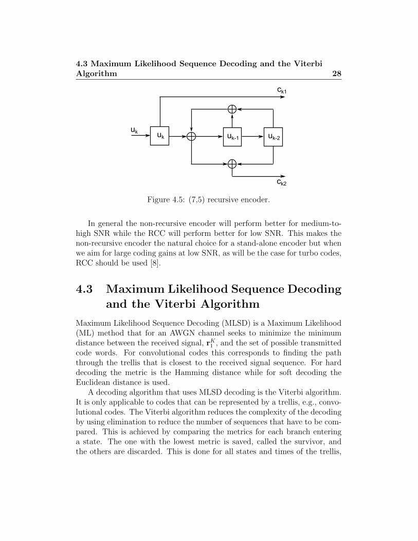
Figure 4.5: (7,5) recursive encoder.
In general the non-recursive encoder will perform better for medium-to-high SNR while the RCC will perform better for low SNR. This makes thenon-recursive encoder the natural choice for a stand-alone encoder but whenwe aim for large coding gains at low SNR, as will be the case for turbo codes,RCC should be used [8].
4.3 Maximum Likelihood Sequence Decoding
and the Viterbi Algorithm
Maximum Likelihood Sequence Decoding (MLSD) is a Maximum Likelihood(ML) method that for an AWGN channel seeks to minimize the minimumdistance between the received signal, rK1 , and the set of possible transmittedcode words. For convolutional codes this corresponds to finding the paththrough the trellis that is closest to the received signal sequence. For harddecoding the metric is the Hamming distance while for soft decoding theEuclidean distance is used.
A decoding algorithm that uses MLSD decoding is the Viterbi algorithm.It is only applicable to codes that can be represented by a trellis, e.g., convo-lutional codes. The Viterbi algorithm reduces the complexity of the decodingby using elimination to reduce the number of sequences that have to be com-pared. This is achieved by comparing the metrics for each branch enteringa state. The one with the lowest metric is saved, called the survivor, andthe others are discarded. This is done for all states and times of the trellis,

4.4 Maximum A-Posteriori Symbol Decoding 29
thereby greatly reducing the complexity of the decoder. This does not affectthe optimality of the decoder since for any future branches through the trel-lis the survivor will still have the lowest metric according to the principle ofoptimality [10].
4.4 Maximum A-Posteriori Symbol Decoding
Another approach to decoding is to minimize the bit error probability ofeach received symbol. One should then aim to maximize the a posterioriprobability (APP) for each bit of the transmitted sequence. This is calledMaximum a Posteriori Probability (MAP) decoding and can be expressed as
uk = argmaxuk
p(uk|rK1 ) = argmaxuk
Pr(uk)p(rK1 |uk)
p(rK1 )(4.22)
∝ argmaxuk
Pr(uk)p(rK1 |uk) (4.23)
The main difference between the Viterbi algorithm and APP algorithms is thetype of output. Whereas Viterbi outputs a hard decision of the transmittedinformation bits the APP algorithm gives the a posteriori probability. The aposteriori probabilities can be interpreted as a soft estimate of the probabilitythat the information bits correspond to a certain input.
4.5 BCJR Algorithm
The BCJR algorithm, named after its inventors: Bahl, Cocke, Jelinek andRaviv, is an optimal decoding method for linear codes which minimizes thesymbol error probability [11]. Unlike the Viterbi algorithm, which minimizesthe probability of word error using ML decoding, BCJR uses the MAP crite-rion. The algorithm is sometimes also called Soft Input Soft Output (SISO)since the information to and from the decoder is soft. The algorithm isderived using the chain rule and Bayes rule iteratively.
Consider the trellis in Figure 4.4 again. A state transition between thestates m′ and m is controlled by the transition probability
Pr(Sk = m|Sk−1 = m′) (4.24)
and the output byp(xk = x|Sk−1 = m′;Sk = m) (4.25)

4.5 BCJR Algorithm 30
The algorithm is based on a forward recursion αk(m), a backward recur-sion βk(m), and a branch metric γk(m′,m). The forward recursion computesthe probability of being in a state, Sk, given that we know all state and tran-sition probabilities up to a time k. The backward recursion is the probabilityof being in the state, Sk, given that we know all state and transition proba-bilities after time k, i.e. for k + 1 to K. The branch metric is a measure ofthe cost of moving from one state Sk to another Sk+1. When these probabil-ities are calculated, the final step is to compute λk(m) and σk(m′,m), whereλk(m) is the probability of being in state m at time k and σk(m′,m) is theprobability of the transition from any state m′ at time k− 1 to a state m atk. In the following sections we will derive the just mentioned probabilities.
4.5.1 A Posteriori Information
The BCJR algorithm uses the observations of the received signal up to timeK, to calculate the APP of the states and transitions [11]. The receivedsignal is represented as K modulated code words
rK1 = (r1, r2, . . . , rK) (4.26)
where the length of each rk is n0. Each node of the trellis in Figure 4.4 isassociated with the APP Pr(Sk = m|rK1 ) and each branch is associated withthe corresponding p(Sk−1 = m′;Sk = m|rK1 ). The aim of the decoder is tocalculate these a posteriori probabilities.
It is easier to derive joint probabilities than to work with the conditionalprobabilities, therefore we introduce
λk(m) = p(Sk = m; rK1 ) (4.27)
andσk(m′,m) = p(Sk−1 = m′;Sk = m; rK1 ) (4.28)
.Since p(rK1 ) is constant for a given rK1 ( p(rK1 ) = λK(0) which is known in
the decoder), we can divide λk(m) and σk(m′,m) with p(rK1 ) to express theAPPs as
Pr(Sk = m|rK1 ) =p(Sk = m; rK1 )
p(rK1 )(4.29)

4.5 BCJR Algorithm 31
p(Sk−1 = m′;Sk = m|rK1 ) =p(Sk−1 = m′;Sk = m; rK1 )
p(rK1 )(4.30)
4.5.2 Derivation of α, β, γ
Let us define the forward and backward recursions and branch metric
αk(m) = p(Sk = m; rk1) (4.31)
βk(m) = p(rKk+1|Sk = m) (4.32)
γk(m′,m) = p(Sk = m; rk|Sk−1 = m′) (4.33)
Nowλk(m) = p(Sk = m; rK1 )p(rKk+1|Sk = m; rk1) (4.34)
Since events after time k are independent of rk1 if Sk is known
λk(m) = αk(m)p(rKk+1|Sk = m)
= αk(m)βk(m). (4.35)
In the same way σk(m′,m) can be expressed as
σk(m′,m) = p(Sk−1 = m′; rk−11 )p(Sk = m; rk|Sk−1 = m′)p(rKk+1|Sk = m)
= αk−1(m′)γk(m′,m)βk(m) (4.36)
In words, to calculate the probability of being in a state m at time k weneed to calculate the cost of being at this state using both the forward andbackward recursions. Similarly, the probability of transitioning from statem′ at time k − 1 to state m at time k is dependent on the cost of being instate m′ at k − 1 obtained using the forwards recursion, the cost of being inm at time k using the backwards recursion and the branch metric associatedwith this branch.
To derive the forward recursion, consider αk(m) for k = 1, 2, . . . , K
αk(m) =M−1∑m′=0
p(Sk−1 = m′;Sk = m; rK1 ) (4.37)

4.5 BCJR Algorithm 32
Similarly as before, if Sk−1 is known, then rk−11 does not affect events aftertime k − 1, so the following can be obtained
αk(m) =∑m′
p(Sk−1 = m′; rk−11 )p(Sk = m; rk|Sk−1 = m′)
=∑m′
αk−1(m′)γk(m′,m) (4.38)
Assuming the code is initialized in the zero state then for k = 0 we have that
α0(0) = 1 (4.39)
α0(m) = 0 , m 6= 0 (4.40)
In the same way we can derive the backward recursion. Consider βk(m)for k = 1, 2, . . . , K − 1
βk(m) =M−1∑m′=0
p(Sk+1 = m′; rKk+1|Sk = m)
=∑m′
p(Sk+1 = m′; rk+1|Sk = m)p(rKk+2|Sk+1 = m′)
=∑m′
βk+1(m′)γk+1(m,m
′) (4.41)
Assuming the code is terminated in the zero state then for k = K we havethe boundary conditions
βK(0) = 1 (4.42)
βK(m) = 0 , m 6= 0 (4.43)
Relations (4.38) and (4.41) show that αk(m) and βk(m) are recursively ob-tained.
The branch metric can be expressed as
γk(m′,m) = p(Sk = m; rk|Sk−1 = m′) (4.44)
= p(Sk = m|Sk−1 = m′)p(rk|Sk = m,Sk−1 = m′) (4.45)
= Pr(uk)p(rk|uk) (4.46)
= Pr(uk)p(rk|xk) (4.47)

4.5 BCJR Algorithm 33
Now, assuming an AWGN channel, we can express
p(rk|xk) =
n0−1∏n=0
p(rnk |xnk) (4.48)
=
n0−1∏n=0
1√2πσ2
exp (− |rnk − xnk |2 1
2σ2) (4.49)
where xnk is the hypothesized received signal belonging to the modulationalphabet. For BPSK modulation the variance is σ2 = N0/2.
4.5.3 Decoding
Minimization of the symbol probability of error is done by determining themost likely input bits, uk from rK1 . Let Ak be the set of transitions corre-sponding to the input being uk = u, where u ∈ {0, 1}. We can then calculate
p(uk = u; rK1 ) =∑
(m′,m)∈A(j)k
σk(m′,m) (4.50)
This is calculated for both p(u = 0; rK1 ) and p(u = 1; rK1 ). In order to obtainthe conditional probability of uk = 1 given rK1 we normalize
Pr(uk = 1|rK1 ) =p(uk = 1; rK1 )
p(uk = 0; rK1 ) + p(uk = 1; rK1 )(4.51)
We can now decode uk = 1 if Pr(uk = 1|rK1 ) ≥ 0.5 and uk = 0 otherwise.
The APP of the encoder output, p(x(j)k = 0; rK1 ) can also be calculated.
Let B(j)k be the set of all transitions from Sk−1 = m′ to Sk = m which
correspond to the jth output digit , x(j)k , being 0. For time-invariant codes,
which will be assumed here, B(j)k is independent of k. Then
p(x(j)k = 0; rK1 ) =
∑(m′,m)∈B(j)
k
σk(m′,m) (4.52)
and this can be normalized similarly to (4.51) in order to form Pr(x(j)k =
1|rK1 ).
4.6 Turbo Codes 34
4.5.4 Outline of the Algorithm
Let us summarize the steps of the algorithm that need to be performed inthe decoder to obtain λk(m) and σk(m′,m).
1. First, α0(m) and βK(m) for m = 0, 1, . . . ,M − 1 are initialized as in(4.39) and (4.42).
2. When the whole sequence r1K is received, γk+1(m,m
′), αk(m) andβk(m) is computed recursively using (4.44), (4.38) and (4.41). The resultsare then stored for all times and states.
3. The decoder then has all information it needs to compute all λk(m)and σk(m′,m) using (4.35) and (4.36).
4. Using the calculated values the decoder can output the APP of theinput sequence, uK
1 , using (4.50) from which hard decisions can be made. Itcan also output the APP of the encoder output sequence xK
1 using (4.52).From the steps above it can be concluded that the algorithm will require
a lot of memory to store all values α, β, and γ. Also since σk and λk aredependent on calculations based on all previous and subsequent k in rK1 theamount of calculations will grow too many if the block lengths and constraintlengths are not kept low.
4.6 Turbo Codes
Berrou et al. introduced turbo codes in 1993 and achieved performance closeto the Shannon limit [12]. Since then further research has resulted in otherturbo-like codes. Turbo codes and turbo-like codes can be viewed as a re-finement of a concatenated encoding structure. For decoding the BCJRalgorithm is used iteratively. The purpose of this section is to explain thebasics needed for understanding such codes.
4.6.1 Concatenated Codes with Interleaver
The performance of a convolutional code is mainly defined by its error correc-tion capability which depends on the minimum distance of the code. Codescan have different lengths for a given code rate, Rc. Longer codes give largerminimum distance and thus offer better performance [9]. However, withincreasing lengths the decoding complexity also increases, generally expo-nentially. A way of obtaining long block lengths and keeping reasonablecomplexity is to concatenate codes with shorter block lengths. The code

4.6 Turbo Codes 35
words of the first encoder will act as the input to the second, and so on,forming increasingly longer code words. In this report only two levels ofconcatenation will be considered. The first encoder will be called the outerencoder and it generates the outer code, co, and the second will be called theinner encoder and it generates the inner code, ci. If the outer encoder hasrate Ro
c = ko/no and the inner encoder Ric = ki/ni then the overall rate of
the concatenated code is simply the product of the two codes [8]:
Rc =kono
kini
= RocR
ic (4.53)
The main advantage of concatenated codes is that the received, con-catenated codewords can be decoded by subsequent decoders. The code isdecoded in the reverse encoding order, i.e. first the inner decoder decodesthe inner code and passes on the result to the outer decoder. This has theeffect of breaking up the large code into several, simpler codes. Codes withsuch encoding and decoding scheme are often referred to as Serially Concate-nated Convolutional Codes (SCCC), an example of which can be observedin Figure 4.6.
CC1 CC2
CC1-1 CC2
-1
u x
n
r
û
mod
demod
Figure 4.6: Communication system using Serially Concatenated Convolu-tional Codes
It has been shown that the optimal decoding solution for concatenatedcodes is to pass the APP from the inner decoder to the outer decoder [8]. Toreach this optimum one therefore needs the demodulator and inner decoderto generate soft outputs.
When Berrou et al. introduced turbo codes one of the key componentswas a concatenated encoding scheme combined with an interleaver. By in-troducing a pseudo-random interleaver Parallel Concatenated Convolutional

4.6 Turbo Codes 36
Codes (PCCC) can be constructed as in Figure 4.7 as well as the more intu-itive serial concatenated codes in Figure 4.8. In the traditional turbo code,introduced by [11], parallel concatenation was used but as interest grew inthe coding community serial concatenation was also utilized in turbo-likecodes [13]. In the PCCC case both encoders use RCC whereas for SCCCsthe outer encoder is non-recursive, non systematic and the inner is RCC. Asmentioned earlier RCCs are suitable when one aims to gain large code gainsat low SNRs.
mod
mod
mod
CC1
CC2
u
n
n
n
Figure 4.7: Transmission system using Parallel Concatenated ConvolutionalCodes with interleaver
CC1 CC2
u x
n
mod
Figure 4.8: Transmission system using Serial Concatenated ConvolutionalCodes with interleaver
For both serial and parallel concatenation the interleaving has the effectof producing codes with very few low-weight codewords. This does not meanthat the free distance of the code is thereby large but does result in thecodewords being relatively sparse and having few nearest neighbors. In otherwords, the coding gain is achieved as result of the interleaver introducing thissparsity, called multiplicity, of codewords of low-weight.

4.6 Turbo Codes 37
The introduction of the interleaver has the side-effect of making the num-ber of possible states for the entire codeword very large. This is the result ofthe interleaver randomly permuting the outer code and feeding this as inputto the inner encoder. Any state diagram over the entire encoding procedurewould hence have to take this into effect and will thereby become impossibleto decode in an optimal way.
4.6.2 Extrinsic Information
An additional performance increasing factor introduced by Berrou et al. isextrinsic information [12]. Extrinsic information can, from an abstract level,be viewed as extra knowledge gained from the decoding process. In practice,this means that the information delivered from the outer to the inner encoderis no longer the APP but extrinsic information formed by the normalizationof the computed APP by its corresponding a priori probability. In otherwords the values are based on information coming from all symbols, exceptthe one corresponding to the same symbol. A trivial way of realizing this isby modifying the APP output as
Pr(uk = 1|rK1 )′= Pr(uk = 1|rK1 )/Pr(uk = 1). (4.54)
Pr(uk = 1|rK1 )′will then be the extrinsic output. The division by Pr(uk = 1)
can however result in numerical problems, especially for the last iterationswhere the a priori values can approach 0. An alternate solution to this isto not include the a priori values when calculating the γk(m′,m) used tocalculate σk(m′,m) [14]. This is expressed as
γ′k(m′,m) = p(rk|xk) (4.55)
and σ′k(m′,m) can now be expressed as
σ′k(m′,m) = αk−1(m′)γ′k(m′,m)βk(m) (4.56)
The extrinsic output can now be obtained by modifying (4.50) as
p(uk = u; rK1 )′=
∑(m′,m)∈A(j)
k
σ′k(m′,m) (4.57)
and from this Pr(uk = 1|rK1 )′
can be formed through normalization as in(4.51).

4.6 Turbo Codes 38
4.6.3 Iterative Decoding
Since the large number of states in turbo and turbo-like codes make optimaldecoding impossible, Berrou et al. introduced a suboptimal iterative decod-ing algorithm, known as the turbo decoding algorithm. This algorithm wasbased on iteratively using concatenated and locally optimal decoders basedon the BCJR algorithm. This eventually results in an APP estimate of thetransmitted information bits. Since there exists both parallel and serial en-coder schemes there are also parallel and serial decoder schemes. They bothuse the same decoding principles, albeit in different configurations, and henceonly one will be explained in any detail in this report. The decoder for theserially concatenated code tends to be somewhat simpler to describe and isthereby chosen here.
The inner decoder feeds the the outer decoder with extrinsic informationcalculated from the received signal and a priori values. The outer decodercalculates the APP of the outer encoder output for each iteration and feedsthis back to the inner decoder in the subsequent iteration, where it is usedas a priori values.
The SCCC decoding scheme can be observed in Figure 4.9. If the feedbackis disregarded one can observe that for each operation in the encoder thereis an inverse operation in the decoder. The order of the decoding operationsis also the reverse of the encoder.
CC1 CC2
CC1-1 CC2
-1
u x
n
r
û
APPe a priori
mod
-1ĉ' ĉ
c c'
demod
Figure 4.9: Serially Concatenated Convolutional Turbo-like code
The inner decoder receives the soft-valued symbol sequence, rK1 and usesthis information to compute all γ′-values according to (4.55). Since γ′ is notdependent on the a priori probabilities this can be calculated once for eachreceived sequence and then stored. With all γ′ calculated the decoder can,

4.6 Turbo Codes 39
for each iteration, calculate the γ-values as
γk(m′,m) = Pr(uk)γ′k(m′,m). (4.58)
During the first iteration the a priori probability used for these calculationsis unknown and is hence set to 0.5 if one uses the probability domain. Theα- and β-values can now be calculated according to (4.38) and (4.41). Nowσ′ can be calculated according to (4.56). With σ′ calculated the extrinsicinformation output, called c′ in Figure 4.9, can be computed according to(4.57).
Thereafter, c′ is de-interleaved to generate c which is used by the outerdecoder. Here one cannot use the BCJR algorithm exactly as in the innerdecoder. Since the input now is a probability the branch cost has to becalculated differently. The γ-value is obtained according to
γk(m′,m) =
n0−1∏n=0
Pr(c(n)k = c(n)(m′,m)) (4.59)
where c(n)(m′,m) ∈ {0, 1} is the code bit n associated with the trellis tran-sition (m′,m). In other words
Pr(c(n)k = c(n)(m′,m)) =
{c(n)k , c(n) = 1
1− c(n)k , c(n) = 0(4.60)
This γ will have to be re-calculated for each iteration since it is dependenton c which varies for each iteration. After this the decoding algorithm canfunction as in the inner decoder and calculate α, β, and σ. From σ the APP-values of the inserted information bits can be formed using (4.50). Fromthese the most likely bits for this iteration can be computed. The γ valuesare also used to calculate the APP of the outer encoder output according to(4.52). This is then interleaved to form the a priori information and a newiteration is begun. In the new iteration these priors are now used by the innerdecoder in (4.44). Except for this difference everything else is done in thesame manner as in the first iteration. This iterative process continues untila fixed number of iterations have been performed or some stopping criterionhas been met. After this the APP-values of the input bits for this iterationare returned and decisions can be performed on these to form uK
1 .For PCCC turbo codes the basics of the algorithm are similar but there
are some differences to take into consideration. These differences are related
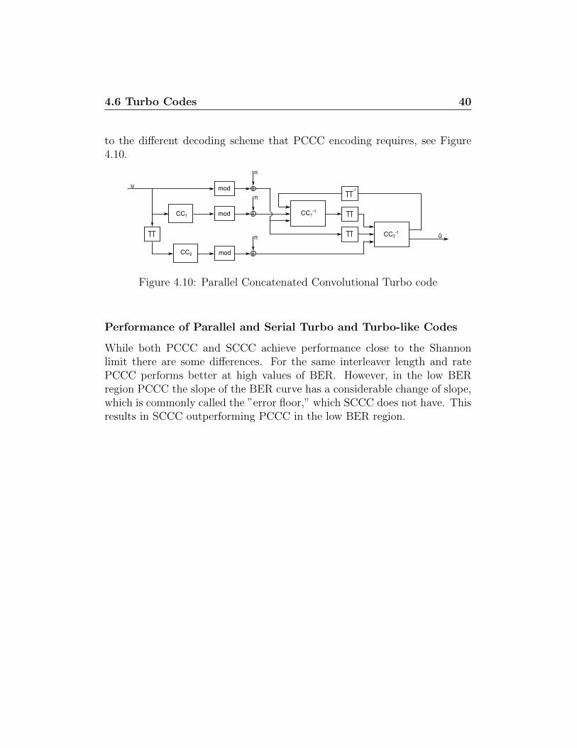
4.6 Turbo Codes 40
to the different decoding scheme that PCCC encoding requires, see Figure4.10.
mod
mod
mod
CC1-1
CC2-1
-1
CC1
CC2
u
n
n
n û
Figure 4.10: Parallel Concatenated Convolutional Turbo code
Performance of Parallel and Serial Turbo and Turbo-like Codes
While both PCCC and SCCC achieve performance close to the Shannonlimit there are some differences. For the same interleaver length and ratePCCC performs better at high values of BER. However, in the low BERregion PCCC the slope of the BER curve has a considerable change of slope,which is commonly called the ”error floor,” which SCCC does not have. Thisresults in SCCC outperforming PCCC in the low BER region.

Chapter 5
Implementation and Results
The IT++ turbo decoder that is wrapped using SWIG is not a stand aloneclass. It requires other functions such as modulation, adding noise and count-ing errors in order for any results to be obtained. It also requires the correctparameters to be passed to it, such as the noise variance and the generatorvectors. Since it functions at such low BER one also needs to send it largeamounts of information bits in order for the simulation results to be statisti-cally sound. To make sure all this would not cause problems once the IT++turbo decoder was successfully wrapped, a Monte Carlo loop with an SCCCturbo-like decoder was implemented in Python beforehand. The main file iscalled turbo.py, see Appendix B.2.1.
The Monte Carlo loop has two stopping criteria: it has to have processedat least a certain amount of blocks and a certain amount of errors. The firstcriterion will ensure that at least some blocks are used when the BER ishigh, otherwise all errors could occur in a single block. The second criterionguarantees that for low BER, enough blocks are sent so that the results arestatistically meaningful.
With the Monte Carlo loop tested and completed the SCCC turbo-likeencoder and decoder were implemented. What we wanted to achieve was aPython code that shows the BER for each SNR value and each iteration thedecoder performs.
The Python code is implemented in such a manner that it is possible toreplace and re-use the different functions. In order to show how SWIG canbe used interactively with Python the encoder and decoder were replacedwith the IT++ encoder and decoder functions. These functions are a partof the class Turbo Codec and in order to integrate them with Python the

5.1 Wrapping IT++ 42
Figure 5.1: BER plot for recursive [14,15] turbo code.
class needed to be wrapped. The results of running this Monte Carlo loopare presented in Figure 5.1. The simulated code is a recursive [14,15] turbocode with interleaver size 16384.
5.1 Wrapping IT++
The main problem encountered when trying to wrap the class Turbo Codec
was to wrap the special data structures that IT++ defines. Let us illustratethe problem with an example.
Turbo Codec contains an encoder whose function declaration looks like
void encode ( const bvec &input , bvec &output )
The arguments to the function are references to the type bvec which is abinary vector. This vector is not a standard C++ data structure but isdefined by IT++. Therefore we cannot pass the values from Python toSWIG as is the case when we have an int or double, etc. Since SWIG doesnot recognize these special data types and cannot perform a standard typeconversion they have to be handled separately.
Assume we have generated a bit sequence in Python that is of the datastructure list . Now, we want to pass this to the IT++ encoder but in orderto do that the list first has to be converted to a standard C++ data type
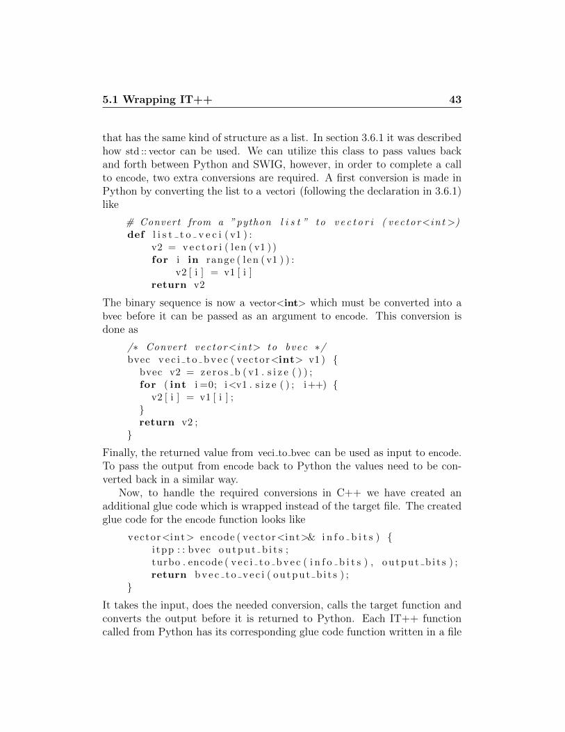
5.1 Wrapping IT++ 43
that has the same kind of structure as a list. In section 3.6.1 it was describedhow std :: vector can be used. We can utilize this class to pass values backand forth between Python and SWIG, however, in order to complete a callto encode, two extra conversions are required. A first conversion is made inPython by converting the list to a vectori (following the declaration in 3.6.1)like
# Convert from a ”python l i s t ” to v e c t o r i ( vec tor<in t >)def l i s t t o v e c i ( v1 ) :
v2 = ve c t o r i ( l en ( v1 ) )for i in range ( l en ( v1 ) ) :
v2 [ i ] = v1 [ i ]return v2
The binary sequence is now a vector<int> which must be converted into abvec before it can be passed as an argument to encode. This conversion isdone as
/∗ Convert vec tor<in t> to bvec ∗/bvec v e c i t o bv e c ( vector<int> v1 ) {
bvec v2 = ze ro s b ( v1 . s i z e ( ) ) ;for ( int i =0; i<v1 . s i z e ( ) ; i++) {
v2 [ i ] = v1 [ i ] ;}return v2 ;
}
Finally, the returned value from veci to bvec can be used as input to encode.To pass the output from encode back to Python the values need to be con-verted back in a similar way.
Now, to handle the required conversions in C++ we have created anadditional glue code which is wrapped instead of the target file. The createdglue code for the encode function looks like
vector<int> encode ( vector<int>& i n f o b i t s ) {i tpp : : bvec ou tpu t b i t s ;turbo . encode ( v e c i t o bv e c ( i n f o b i t s ) , ou tpu t b i t s ) ;return bv e c t o v e c i ( ou tpu t b i t s ) ;
}
It takes the input, does the needed conversion, calls the target function andconverts the output before it is returned to Python. Each IT++ functioncalled from Python has its corresponding glue code function written in a file

5.1 Wrapping IT++ 44
called demo.cc. Two files, converters .h and converters .py, with all requiredconverters have been created, see Appendix B.1.7 and B.1.8. Figure 5.2shows how these files are used by the C++ and Python modules.
converters.h
demo.cc
converters.py
turbo.pySWIG
Figure 5.2: Dependencies between converters and C++ and Python modules.
Let us now summarize what we have done. Since IT++ uses its owndefined data structures we cannot wrap the IT++ classes and functions di-rectly. Instead we have created a glue code called demo.cc which is wrappedinstead. This glue code contains functions that call the IT++ functions andincludes converters .h.
The file which implements the Monte Carlo loop is turbo.py. It is alsothe file that includes the SWIG generated Python module which enablescalls to demo.cc. It uses converters .py for handling non-standard C++ datastructures, such as list (), to demo.cc.
An alternative and more complex way to handle the IT++ data types isto write a library similar to std vector . i. However, we will begin with usingconverters .h and converters .py since the main task is to determine whetherBCL can be wrapped by SWIG or not.
5.1.1 Libraries
IT++ uses the libraries Basic Linear Algebra Subprograms (blas), Com-plex Basic Linear Algebra Subprograms (cblas), Linear Algebra PACKage(LAPACK), and Fastest Fourier Transform in the West (fftw), thereforethese have to be included in the setup file. The libraries blas, cblas, andLAPACK all give support for linear algebra operations, whereas fftw is usedfor computing discrete Fourier transforms.

5.2 Wrapping BCL 45
5.2 Wrapping BCL
The previous section showed how classes in IT++ can be wrapped. The goalof this thesis however is to wrap a class in BCL.
Due to the Ericsson confidentiality policy we will not mention the realname of the class or any variables but only show examples that describe theprinciples behind certain code sections of the class. For the sake of simplicitywe will refer to the class as bcl class .
We have already seen how classes can be wrapped using converters .h.However, writing glue code can be somewhat inefficient and cumbersome. Abetter way would be to wrap a BCL class without using any glue code. Sucha solution would require a library similar to std vector . i, as mentioned insection 3.6.1, but written for IT++ data types. This is however not in thescope of this thesis. Instead, the aim is to examine whether it is possible at allto wrap a BCL class. An attempt to wrap the BCL class directly was madebut this was prevented by protected sections in bcl class . Generally, SWIGdoes not support protected or private declarations and simply ignores thesekind of sections [3]. The program will run until the protected variable is usedand then generate an error message about an unknown variable.
Since the BCL class cannot be wrapped without glue code it has beenwrapped in the same way as for IT++ where converters .h and converters .py
are used for passing IT++ data structures between C++ and Python.The main problem encountered when wrapping bcl class was to wrap
namespaces. To illustrate, consider the following header file
/∗ Header f i l e ns example . h ∗/
#inc lude ”b . h”
namespace a {using namespace b ;
}
In normal C++ code this will function without any problem if the declarationof b is written in b.h. However, in SWIG this would give the error message
Error : Nothing known about namespace ’ b ’
The preprocessor simply ignores the namespace declaration in b.h. A work-around to this problem is to add %include b.h before %include ns example.h

5.2 Wrapping BCL 46
in the interface file. This solution is based on making sure that SWIG seesthe declaration of namespace b before it processes ns example.h.
The same error will be generated if namespace b is not defined. This canbe solved by defining the namespace in the interface file like
/∗ I n t e r f a c e f i l e ns example . i ∗/
%module ns example
%{#include ”ns example . h”%}
namespace b {} ;
%inc lude ”ns example . h”
With the solutions converters .h, converters .py, and glue code it is possible towrap BCL.

Chapter 6
Discussion and Conclusion
The result of having a C++ function wrapped using SWIG and having itaccessible in Python can be very useful. The interactivity of Python is com-bined with the flexibility and fast execution time of C++. As can be seenfrom our example of wrapping the IT++ turbo class, SWIG enables a veryconvenient way of interacting with a C++ class from Python. The parame-ters can be quickly altered without the need to recompile. The resulting dataof the C++ class is then available and can be manipulated and presented inPython.
If the library to be wrapped has few dependencies to other libraries andonly contains standard C++ data types, then wrapping with SWIG is ratherstraight forward. The libraries IT++ and BCL however use IT++ defineddata structures which introduces additional complexity. A favorable solutionto handle these data structures would be a library similar to std vector . i.However, BCL includes protected sections which SWIG does not support,therefore such a solution is not applicable in this case. Instead we haveimplemented a solution to cope with the restraints of BCL. It was achieved,not by wrapping the functions/classes themselves but rather by wrappingwritten glue code for each function/class.
In order to pass special data types between Python and C++ the createdfiles converters .h and converters .py are used. This solution is somewhat cum-bersome. Since Python is a typeless language the user needs to understandwhat data types are used by the functions and make the appropriate typeconversions. Although writing this glue code might seem ponderous, it onlyneeds to be done once. To decide whether it is beneficial to wrap modules inthis way one should consider the amount of time and effort that is required

48
to write the glue codes compared to the amount of usage. To give an ex-ample, consider the IT++ turbo code. If we would have implemented theMonte Carlo loop in C++, re-compilation would have been needed even af-ter the slightest change, such as changing generator vectors. Since Python isinterpreted, by implementing the Monte Carlo loop in Python and importingthe wrapped IT++ turbo code, we would avoid these re-compilations. If theturbo code will have to changed only a couple of times then maybe wrappingit will not be beneficial. However, if it will be altered often, perhaps in atesting environment, then using SWIG can have great advantages.
SWIG gives support for most standard C++ directives. There are how-ever some limitations, such as that SWIG generally cannot handle privateor protected sections. This can be seen as a flaw of the tool, given thatthese kind of data types are commonly used. There are work-arounds to thisproblem, but it requires additional effort and knowledge from the user (suchas writing glue code). Ideally SWIG should handle this for the user. Apartfrom protected sections, if we consider the fact that BCL uses non standardC++ data types a solution similar to std vector . i should be possible. Thiswould remove the need for any glue code to be written by the user and wouldthereby bring out the full potential of SWIG.

Bibliography
[1] “About it++.” http://itpp.sourceforge.net/current/index.html [Ac-cessed 19 May 2011].
[2] “Templates.” http://www.cplusplus.com/doc/tutorial/templates/ [Ac-cessed 19 May 2011].
[3] D. M. Beazley, “Swig-2.0 documentation.” http://www.swig.org/Doc2.0/SWIGDocumentation.pdf [Accessed 1 June 2011].
[4] J. K. Ousterhout, “Scripting: Higher level programming for the 21stcentury,” IEEE Computer magazine, 1998.
[5] “Distutils.” http://docs.python.org/distutils/setupscript.html [Ac-cessed 19 May 2011].
[6] D. M. Beazley, “Swig-2.0 library.” http://www.swig.org/Doc2.0/Library.html[Accessed 1 June 2011].
[7] C. Schlegel and L. C. Perez, Trellis Coding. Lightning Source Inc, 1997.
[8] S. Benedetto and E. Biglieri, Principles of Digital Transmission WithWireless Applications. Kluwer Academic/Plenum Publishers, 1999.
[9] J. G. Proakis and M. Salehi, Digital Communications. McGraw-Hill,5th ed., 2008.
[10] U. Madhow, Fundamentals of Digital Communications. Cambridge Uni-versity Press, 2008.
[11] L. R. Bahl, J. Cocke, F. Jelinek, and J. Raviv, “Optimal decoding oflinear codes for minimizing symbol error rate,” IEEE Transactions onInformation Theory, vol. 20, pp. 284–287, March 1974.
BIBLIOGRAPHY 50
[12] C. Berrou, A. Glavieux, and P. Thitimajshima, “Near shannon limiterror-correcting coding and decoding,” in Proc. IEEE InternationalConference on Communications, pp. 1064–1070, May 1993.
[13] S. Benedetto, D. Divsalar, G. Montorsi, and F. Pollara, “Serial concate-nation of interleaved codes: Performance analysis, design, and iterativedecoding,” IEEE Trans. Inform. Theory, vol. 44, pp. 909–926, 1998.
[14] S. Benedetto, D. Divsalar, F. Ieee, G. Montorsi, and F. Pollara, “A soft-input soft-output app module for iterative decoding of concatenatedcodes,” IEEE Commun. Lett, vol. 1, pp. 22–24, 1997.
[15] “Install it++.” http://itpp.sourceforge.net/stable/installation.html[Accessed 6 June 2011].
[16] “Install swig.” http://sourceforge.net/projects/swig/files/swig/ [Ac-cessed 6 June 2011].
[17] “install python.” http://diveintopython3.org/installing-python.html#ubuntu [Accessed 9 June 2011].
[18] “Numpy.” http://sourceforge.net/projects/numpy/files/NumPy/ [Ac-cessed 9 June 2011].

Acronyms
API Application Programming Interface
APP a posteriori probability
AWGN Additive White Gaussian Noise
BCL Baseband Core Library
BER Bit Error Rate
blas Basic Linear Algebra Subprograms
BPSK Binary Phase Shift Keying
cblas Complex Basic Linear Algebra Subprograms
fftw Fastest Fourier Transform in the West
LAPACK Linear Algebra PACKage
MAP Maximum a Posteriori Probability
ML Maximum Likelihood
MLSD Maximum Likelihood Sequence Decoding
OS Operating System
PCCC Parallel Concatenated Convolutional Codes
RCC Recursive Convolution Codes
SCCC Serially Concatenated Convolutional Codes

BIBLIOGRAPHY 52
SISO Soft Input Soft Output
SNR Signal to Noise Ratio
STL Standard Template Library
SWIG Simplified Wrapper Interface Generator

Appendix A
User’s Guide
This guide describes the steps required to wrap the encode() function in IT++with SWIG and integrate it with Python. Installations vary depending onthe used Operating System (OS). These instructions are written for LinuxUbuntu.
A.1 Setup
Before writing any code we need to install all required software.1. Install IT++ following the instructions in [15].2. Install SWIG. Most popular Linux distributions come with SWIG but
the version may vary depending on which distribution. The version used inthis thesis is 2.0.1 and it can be downloaded from [16].
3. Install Python. Most popular Linux distributions come with Pythonbut the version may vary depending on which distribution. The version usedin this thesis is 3.1.1 Follow the instructions in [17] to install. The numpy
package is needed in order to use functions such as rand(), sqrt(), etc. Version1.6.0 is compatible with Python 3.x and can be found at [18].
A.2 Wrap
With all tools installed we can now start to wrap.1. Create the interface file, see section 3.2.1 and appendix B.1.3. De-
pending on what type of data structures we want to pass between Python

A.2 Wrap 54
and C++ other instantiations of std :: vector can be made. New converterscan be written using std :: vector.
2. Create the glue code and the corresponding header file for the cho-sen target function, see section 5.1, appendix B.1.1 and B.1.2. Make sureconverters .h is included in the .cc-file.
3. Write the setup file, see section 3.2.2 and appendix B.1.4. As men-tioned in section 3.2.2 there are two ways to generate the extension module.Here we use the second mentioned method, therefore, give the interface file,target file and converters file as input to sources. When including libraries,make sure they are built with the same gcc compiler version as the one usedfor running SWIG.
4. Run the following command to generate the wrapper, python moduleand shared library:
python setup . py bu i l d ex t −−i np l a c e
5. We can now import the python module into Python and use it togetherwith converters .py to pass data to the wrapped function. This can be donein the command prompt like
>>>from demo import ∗>>>from conve r t e r s import ∗
or it can be included into a .py-file, see appendix B.1.5.

Appendix B
Code
B.1 SWIG modules
B.1.1 demo.cc
/∗∗ The func t i on s in t h i s f i l e a c t s as g l u e code f o r c a l l i n g IT++ func t i on s .
∗/
#include <iostream>#include <s t r i ng>#include <vector>#include < i t b a s e . h>#include <bc l . h>#include ” turbo . h”#include ”modulator . h”#include ” e r r o r c oun t e r s . h”#include ”demo . h”#include ” conve r t e r s . h”
using namespace std ;
// Globa l o b j e c t si tpp : : Turbo Codec turbo ;
/∗∗ Ca l l s the IT++ func t i on decode@param rec A vec to r con ta in ing r e c e i v ed data@return A vec to r con ta in ing the decoded r e c e i v ed data

B.1 SWIG modules 56
∗/vector<int> decode ( vector<double> r e c ) {
i tpp : : bvec d e c b i t s ;i tpp : : i v e c i t e r ;turbo . decode ( vecd to vec ( r ec ) , d e c b i t s , i t e r ) ;return bv e c t o v e c i ( d e c b i t s ) ;
}
/∗∗ Ca l l s the IT++ func t i on encode@param i n f o b i t s A vec to r con ta in ing in format ion b i t s@return A vec to r con ta in ing the encoded in format ion b i t s
∗/vector<int> encode ( vector<int>& i n f o b i t s ) {
i tpp : : bvec ou tpu t b i t s ;turbo . encode ( v e c i t o bv e c ( i n f o b i t s ) , ou tpu t b i t s ) ;return bv e c t o v e c i ( ou tpu t b i t s ) ;
}
/∗∗ Ca l l s the IT++ func t i on wcdma turbo in t e r l eave r s equence@param n In t e r l e a v e r l e n g t h@return A vec to r con ta in ing the i n t e r l e a v e r sequence
∗/vector<int> g e t i n t e r l e a v e r ( int n) {
return i v e c t o v e c i ( i tpp : : wcdma turbo inte r l eaver sequence ( n) ) ;
}
/∗∗ Ca l l s the IT++ func t i on se t paramete r s . I n i t i a l i z e turbo f o rl o g max decoding@param gen1 A vec to r con ta in ing the genera tor po lynomia l s
f o r the f i r s t c on s t i t u en t encoder@param gen2 A vec to r con ta in ing the genera tor po lynomia l s
f o r the second con s t i t u en t encoder@param con s t r a i n t l e n g t h The con s t r a i n t l e n g t h o f the two
con s t i t u en t encoders@param i n t e r l e a v e r I n t e r l e a v e r sequence@param i n i t e r a t i o n s The number o f decoding i t e r a t i o n s@param in l o gmax s c a l e f a c t o r This parameter a l l ow s f o r a
down−s c a l i n g o f the e x t r i n s i c in format ion t ha t w i l l bepassed on to the next decoder
∗/void i n i t turbo max ( vector<s t r i ng>& gen1 , vector<s t r i ng>& gen2 ,

B.1 SWIG modules 57
int c on s t r a i n t l e n g t h , vector<int>& in t e r l e a v e r , inti t e r a t i o n s , double i n l o gmax s c a l e f a c t o r ) {
i tpp : : i v e c gen1 ive c = v e c s t o i v e c ( gen1 ) ;i tpp : : i v e c gen2 ive c = v e c s t o i v e c ( gen2 ) ;i tpp : : i v e c i n t e r l e a v e r i v e c = v e c i t o i v e c ( i n t e r l e a v e r ) ;turbo . s e t paramete r s ( gen1 ivec , gen2 ivec , c on s t r a i n t l eng th ,
i n t e r l e a v e r i v e c , i t e r a t i o n s , ”LOGMAX” ,i n l o gmax s c a l e f a c t o r ) ;
}
/∗∗ Ca l l s the IT++ func t i on se t paramete r s . I n i t i a l i z e turbo f o rl o g map decoding@param gen1 A vec to r con ta in ing the genera tor po lynomia l s
f o r the f i r s t c on s t i t u en t encoder@param gen2 A vec to r con ta in ing the genera tor po lynomia l s
f o r the second con s t i t u en t encoder@param con s t r a i n t l e n g t h The con s t r a i n t l e n g t h o f the two
con s t i t u en t encoders@param i n t e r l e a v e r I n t e r l e a v e r sequence@param i n i t e r a t i o n s The number o f decoding i t e r a t i o n s
∗/void i n i t turbo map ( vector<s t r i ng>& gen1 , vector<s t r i ng>& gen2 ,
int c on s t r a i n t l eng th , vector<int>& in t e r l e a v e r , inti t e r a t i o n s ) {
i tpp : : i v e c gen1 ive c = v e c s t o i v e c ( gen1 ) ;i tpp : : i v e c gen2 ive c = v e c s t o i v e c ( gen2 ) ;i tpp : : i v e c i n t e r l e a v e r i v e c = v e c i t o i v e c ( i n t e r l e a v e r ) ;turbo . s e t paramete r s ( gen1 ivec , gen2 ivec , c on s t r a i n t l eng th ,
i n t e r l e a v e r i v e c , i t e r a t i o n s , ”LOGMAP” ) ;}
/∗∗ Set s c a l i n g f a c t o r@param Lc Sca l ing f a c t o r
∗/void s e t s c a l e f a c t o r (double Lc ) {
turbo . s e t s c a l i n g f a c t o r (Lc ) ;}
B.1.2 demo.h
#include <vector>using namespace std ;

B.1 SWIG modules 58
vector<int> decode ( vector<double> r e c ) ;vector<int> encode ( vector<int>& i n f o b i t s ) ;vector<int> g e t i n t e r l e a v e r ( int n) ;void i n i t turbo max ( vector<s t r i ng>& gen1 , vector<s t r i ng>& gen2 ,
int c on s t r a i n t l eng th , vector<int>& in t e r l e a v e r , inti t e r a t i o n s , double i n l o gmax s c a l e f a c t o r ) ;
void i n i t turbo map ( vector<s t r i ng>& gen1 , vector<s t r i ng>& gen2 ,int c on s t r a i n t l eng th , vector<int>& in t e r l e a v e r , inti t e r a t i o n s ) ;
void s e t s c a l e f a c t o r (double Lc ) ;
B.1.3 demo.i
%module demo
%inc lude ” s t d s t r i n g . i ”%inc lude ” s t d v e c t o r . i ”
%{#include < i t b a s e . h>#include ”demo . h”%}
// I n s t a n t i a t i o n s o f v e c t o r ( s t d v e c t o r . i )namespace std {
%template ( v e c t o r i ) vector<int >;%template ( vectord ) vector<double>;%template ( v e c t o r s ) vector<std : : s t r i ng >;} ;
%inc lude ”demo . h”
B.1.4 setup.py
from d i s t u t i l s . core import ∗demo module = Extension (
’ demo ’ ,s ou r c e s = [ ’demo . i ’ , ’demo . cc ’ , ’ c onve r t e r s . cc ’ ] ,
i n c l u d e d i r s = [ ’ example/path/ to / inc lude / f i l e / ’ ] ,
l i b r a r y d i r s =[ ’ example/path/ to / l i b r a r y / ’ ] ,
l i b r a r i e s =[ ’ lapack ’ , ’ b l a s ’ , ’ f f tw3 ’ , ’ cb l a s ’ , ’ i tpp−ex t e rna l ’ , ’lapack−noopt ’ , ’ g f o r t r an ’ , ’ i tpp ’ ] ,

B.1 SWIG modules 59
sw ig opt s=[”−c++” ])setup (
name = ’demo ’ ,v e r s i on = ’ 3 .0 ’ ,author = ”Oskar Arivdsson Tjader , Linh Tran” ,d e s c r i p t i o n = ” swig demo us ing IT++” ,ext modules = [ demo module ] ,py modules = [ ”demo” ]
)
B.1.5 turbo.py
# Note : The IT++ decoder does not return the d i f f e r e n t BER foreach i t e r a t i o n but only for the l a s t . S ince we want to showi t s performance for each i t e r a t i o n and SNR value we need toi n s t a n t i a t e a new decoder for each i t e r a t i o n o f each \ac{SNR}to get around this
from demo import ∗from conve r t e r s import ∗
from he lp func s import ∗from com funcs import∗from he lp func s import∗
from numpy import array
de f main ( ) :
BLOCK SIZE = 16384c on s t r a i n t l e n g t h = 4gen = ( ’ 013 ’ , ’ 015 ’ )metr ic = ’LOGMAP’l o g s c a l e f a c t o r = 0 .7
SNR dB min = 0 # min SNRSNR dB max = 50 # max SNRSNR dB step = 5 # SNR granu l a r i t yEb = 1 # Bit ( symbol ) energy
MIN NO ERRORS = 100 # Limit for number o f e r r o r s (monte c a r l o )
MIN NO BLOCKS = 100 # Limit for number o f

B.1 SWIG modules 60
t ransmit ted b locks (monte c a r l o )ITERATIONS = 12 # No o f i t e r a t i o n s in turbo
decoder
SNR dB vec = range (SNR dB min , SNR dB max + SNR dB step ,SNR dB step )
SNR dB vec real = array ( SNR dB vec , f loat ) /100
# generate i n t e r l e a v e ri n t e r l e a v e r = l i s t t o v e c i ( g e t i n t e r l e a v e r (BLOCK SIZE) )
for SNR idx in SNR dB vec real :len sym=49164ra t e = BLOCK SIZE/ len symSNR linear = pow(10 , SNR idx /10)N0 = (1/ SNR linear ) / ra t evar=N0/2
for i t e r a t i o n in range (ITERATIONS) :
random . seed (1 )g en ve c i = l i s t t o v e c s ( gen )i f ( metr ic ==’LOGMAX’ ) :
in i t turbo max ( gen vec i , gen vec i ,c on s t r a i n t l eng th , i n t e r l e a v e r ,i t e r a t i o n +1, metric , l o g s c a l e f a c t o r)
else :i n i t turbo map ( gen vec i , gen vec i ,
c on s t r a i n t l eng th , i n t e r l e a v e r ,i t e r a t i o n +1, metr ic )
# Generate in fo rmat ion b i t si n f o b i t s =l i s t t o v e c i ( c r e a t e da ta (BLOCK SIZE) )
# Encode in fo rmat ion b i t sou tpu t b i t s = l i s t t o v e c i ( encode ( i n f o b i t s ) )
# Modulate b i t ssymbols = modulate ( ou tpu t b i t s )
r a t e = ( f loat (BLOCK SIZE) / l en ( symbols ) )No err = 0no b locks = 0

B.1 SWIG modules 61
while ( No err < MIN NO ERRORS) or ( no b locks <MIN NO BLOCKS) :
no i s e = create AWGN( len sym , var )r ec = l i s t t o v e c d ( symbols + no i s e )
#s e t s c a l e f a c t o rs c a l e f a c t o r = 4/N0s e t s c a l e f a c t o r ( s c a l e f a c t o r )
# Decode r e c i v ed symbolsd e c b i t s = decode ( r ec )
# Count e r r o r sNo err += coun t e r r o r s ( i n f o b i t s ,
d e c b i t s )no b locks += 1
ber = No err /( no b locks ∗BLOCK SIZE)pr in t ( ”SNR : ” , SNR idx )p r i n t ( ” i t e r a t i o n : ” , i t e r a t i o n +1)p r in t ( ” BER : ” , ber )f i l ename=’BER’+metr ic+’ . txt ’with open ( f i l ename , mode=’ a ’ , encoding=’ utf−8 ’ )
as a f i l e :a f i l e . wr i t e ( ” ” + s t r ( ber ) )
B.1.6 converters.cc
/∗∗ This f i l e con ta ins f unc t i on s f o r conve r t a t i on between i t p p : :Vec<Type> and s t d : : vec tor<Type>
∗/
#include <vector>using namespace std ;#include ” conve r t e r s . h”
/∗∗ Convert v e c t o r o f type i t p p : : bvec to s t d : : vec tor<in t>∗ @param v1 vec to r o f b i n a r i e s∗ @return vec t o r∗/vector<int> bv e c t o v e c i ( i tpp : : bvec v1 ) {
vector<int> v2 ;for ( int i =0; i<v1 . s i z e ( ) ; i++) {

B.1 SWIG modules 62
v2 . push back ( v1 [ i ] ) ;}return v2 ;
}
/∗∗ Convert v e c t o r o f type i t p p : : i v e c to s t d : : vec tor<in t>∗ @param v1 vec to r o f i n t e g e r s∗ @return vec t o r∗/vector<int> i v e c t o v e c i ( i tpp : : i v e c v1 ) {
vector<int> v2 ;for ( int i =0; i<v1 . s i z e ( ) ; i++) {
v2 . push back ( v1 [ i ] ) ;}return v2 ;
}
/∗∗ Convert v e c t o r o f type i t p p : : vec to s t d : : vec tor<double>∗ @param v1 vec to r o f decimal va l u e s∗ @return vec t o r∗/vector<double> vec to vecd ( i tpp : : vec v1 ) {
vector<double> v2 ;for ( int i =0; i<v1 . s i z e ( ) ; i++) {
v2 . push back ( v1 [ i ] ) ;}return v2 ;
}
/∗∗ Convert v e c t o r o f type s t d : : vec tor<in t> to i t p p : : bvec∗ @param v1 vec to r o f i n t e g e r s∗ @return vec t o r∗/i tpp : : bvec v e c i t o bv e c ( vector<int> v1 ) {
i tpp : : bvec v2 = itpp : : z e r o s b ( v1 . s i z e ( ) ) ;for ( int i =0; i<v1 . s i z e ( ) ; i++) {
v2 [ i ] = v1 [ i ] ;}return v2 ;
}
/∗∗ Convert v e c t o r o f type s t d : : vec tor<in t> to i t p p : : i v e c∗ @param v1 vec to r o f i n t e g e r s∗ @return vec t o r∗/

B.1 SWIG modules 63
i tpp : : i v e c v e c i t o i v e c ( vector<int> v1 ) {i tpp : : i v e c v2 = itpp : : z e r o s i ( v1 . s i z e ( ) ) ;for ( int i =0; i<v1 . s i z e ( ) ; i++) {
v2 [ i ] = v1 [ i ] ;}return v2 ;
}
/∗∗ Convert v e c t o r o f type s t d : : vec tor<s t r i n g> to i t p p : : i v e c∗ @param v1 vec to r o f s t r i n g s∗ @return vec t o r∗/i tpp : : i v e c v e c s t o i v e c ( vector<s t r i ng> v1 ) {
i tpp : : i v e c v2 = itpp : : z e r o s i ( v1 . s i z e ( ) ) ;s t r i n g tmp ;for ( int j =0; j< v1 . s i z e ( ) ; j++){
tmp = ”” ;for ( int i =0; i<v1 [ j ] . s i z e ( ) ; i++) {
tmp += v1 [ j ] [ i ] ;}v2 [ j ] = a t o i (tmp . c s t r ( ) ) ;
}return v2 ;
}
/∗∗ Convert v e c t o r o f type s t d : : vec tor<in t> to i t p p : : vec∗ @param v1 vec to r o f i n t e g e r s∗ @return vec t o r∗/i tpp : : vec v e c i t o v e c ( vector<int> v1 ) {
i tpp : : vec v2 = itpp : : z e r o s ( v1 . s i z e ( ) ) ;for ( int i =0; i<v1 . s i z e ( ) ; i++) {
v2 [ i ] = v1 [ i ] ;}return v2 ;
}
/∗∗ Convert v e c t o r o f type s t d : : vec tor<double> to i t p p : : vec∗ @param v1 vec to r o f doub le∗ @return vec t o r∗/i tpp : : vec vecd to vec ( vector<double> v1 ) {
i tpp : : vec v2 = itpp : : z e r o s ( v1 . s i z e ( ) ) ;for ( int i =0; i<v1 . s i z e ( ) ; i++) {
v2 [ i ] = v1 [ i ] ;

B.1 SWIG modules 64
}return v2 ;
}
B.1.7 converters.h
#include < i t b a s e . h>#include <vector>using namespace std ;
vector<int> bv e c t o v e c i ( i tpp : : bvec v1 ) ; // i t p p : : bvecto vec tor<in t>
vector<int> i v e c t o v e c i ( i tpp : : i v e c v1 ) ; // i t p p : : i v e cto vec tor<in t>
vector<double> vec to vecd ( i tpp : : vec v1 ) ; // i t p p : : vecto vec tor<in t>
i tpp : : bvec v e c i t o bv e c ( vector<int> v1 ) ; // vector<in t>to i t p p : : bvec
i tpp : : i v e c v e c i t o i v e c ( vector<int> v1 ) ; // vector<in t>to i t p p : : i v e c
i tpp : : i v e c v e c s t o i v e c ( vector<s t r i ng> v1 ) ; // vector<s t r i n g> to i t p p : : i v e c
i tpp : : vec v e c i t o v e c ( vector<int> v1 ) ; // vector<in t>to i t p p : : vec
i tpp : : vec vecd to vec ( vector<double> v1 ) ; // vector<f l o a t> to i t p p : : vec
B.1.8 converters.py
from demo import vectori from demo import vectord from demo import vec-tors
# Convert a ”python l i s t ” to v e c t o r i ( vector<int>)# inparam : a l i s t o f i n t e g e r s# return : a vector<int>de f l i s t t o v e c i ( v1 ) :
v2 = ve c t o r i ( l en ( v1 ) )for i in range ( l en ( v1 ) ) :
v2 [ i ] = v1 [ i ]return v2
# Convert a ”python l i s t ” to v e c t o r f ( vector<f loat >)# inparam : a l i s t o f f l o a t s# return : a vector<f loat>de f l i s t t o v e c d ( v1 ) :
v2 = vectord ( l en ( v1 ) )
B.1 SWIG modules 65
for i in range ( l en ( v1 ) ) :v2 [ i ] = v1 [ i ]
return v2
# Convert a ”python l i s t ” to ve c t o r s ( vector<s t r i ng >)# inparam : a l i s t o f s t r i n g s# return : a vector<s t r i ng>de f l i s t t o v e c s ( v1 ) :
v2 = vec to r s ( l en ( v1 ) )for i in range ( l en ( v1 ) ) :
v2 [ i ] = v1 [ i ]return v2
B.1.9 com funcs.py
from he lp func s import ∗
from numpy import arrayfrom numpy import randomfrom numpy import s q r tfrom numpy import z e r o sfrom numpy import t ransposefrom math import c e i l
#−−−−−−−−−−−−−−−−−−−−−−−−−−−−−−−−−−−−−−−−−−−−−−−−−−−−−−−−−−−−−−−−−−−−−−−−−−−−−−−−−−−−−−−−−−−−−−−−−−−−−−−−−−#
# BPSK modulation .# inparam : a b i t# re turn : an i n t (−1 or 1)def BPSK( b i t ) :
return −b i t ∗2 + 1#−−−−−−−−−−−−−−−−−−−−−−−−−−−−−−−−−−−−−−−−−−−−−−−−−−−−−−−−−−−−−−−−−−−−−−−−−−−−−−−−−−−−−−−−−−−−−−−−−−−−−−−−−−#
# Generate stream of ones and zeros , ( normal ly d i s t r i b u t e d ) , e . g. array ( [ 1 , 0 , 1 , 1 , 0 ] )
# inparam : l en g t h o f generated stream# return : array o f ones and zerosdef c r e a t e da ta (n) :
return random . rand int ( 0 , 2 , ( n , ) ) . t o l i s t ( )#−−−−−−−−−−−−−−−−−−−−−−−−−−−−−−−−−−−−−−−−−−−−−−−−−−−−−−−−−−−−−−−−−−−−−−−−−−−−−−−−−−−−−−−−−−−−−−−−−−−−−−−−−−#

B.1 SWIG modules 66
# Generate array wi th AWGN# inparam1 : l en g t h o f generated stream# inparam2 : no i se var iance# return : array o f f l o a t sdef create AWGN(n , var i ance ) :
return s q r t ( var iance ) ∗random . randn (n)#−−−−−−−−−−−−−−−−−−−−−−−−−−−−−−−−−−−−−−−−−−−−−−−−−−−−−−−−−−−−−−−−−−−−−−−−−−−−−−−−−−−−−−−−−−−−−−−−−−−−−−−−−−#
# Hard dec i s i on −1 −> 0 , 1 −> 1# inparam : l i s t o f −1 and 1# return : l i s t o f 1 and 0def hard dec ( data ) :
for i in range ( l en ( data ) ) :i f ( data [ i ]>0) : data [ i ]=1else : data [ i ]=0
return data#−−−−−−−−−−−−−−−−−−−−−−−−−−−−−−−−−−−−−−−−−−−−−−−−−−−−−−−−−−−−−−−−−−−−−−−−−−−−−−−−−−−−−−−−−−−−−−−−−−−−−−−−−−#
# In t e r l e a v e r# inparam : l en g t h o f array# return : l i s t or array wi th i n t e r l e a v e d e lements and array wi th
i nd e c i e sdef g e n i n t e r l e a v e r (n) :
i n t e r l e a v e r=range (n)random . s h u f f l e ( i n t e r l e a v e r )return i n t e r l e a v e r
#−−−−−−−−−−−−−−−−−−−−−−−−−−−−−−−−−−−−−−−−−−−−−−−−−−−−−−−−−−−−−−−−−−−−−−−−−−−−−−−−−−−−−−−−−−−−−−−−−−−−−−−−−−#
# In t e r l e a v e r# inparam : l i s t or array o f i n t s or f l o a t s# re turn : l i s t or array wi th i n t e r l e a v e d e lements and array wi th
i nd e c i e sdef i n t e r l e a v e ( b i t s , i n t e r l e a v e r ) :
b i t s=s t r 2a r r ay ( b i t s )i n t e r l e a v e d b i t s=b i t s [ i n t e r l e a v e r ]return i n t e r l e a v e d b i t s . t o l i s t ( )
#−−−−−−−−−−−−−−−−−−−−−−−−−−−−−−−−−−−−−−−−−−−−−−−−−−−−−−−−−−−−−−−−−−−−−−−−−−−−−−−−−−−−−−−−−−−−−−−−−−−−−−−−−−#
# Dein t e r l e a v e r# inparam1 : l i s t or array o f i n t s or f l o a t s
B.1 SWIG modules 67
# inparam2 : array wi th i n d e c i e s# re turn : l i s t or array wi th d e i n t e r l e a v e d e lementsdef d e i n t e r l e a v e r ( i n t e r l e a v e d b i t s , i n t e r l e a v e r ) :
s t r 2 a r r ay ( i n t e r l e a v e d b i t s )d e i n t e r l e a v e d b i t s=ze ro s ( l en ( i n t e r l e a v e d b i t s ) , f l o a t )d e i n t e r l e a v e d b i t s [ i n t e r l e a v e r ]= i n t e r l e a v e d b i t s
return d e i n t e r l e a v e d b i t s . t o l i s t ( )#−−−−−−−−−−−−−−−−−−−−−−−−−−−−−−−−−−−−−−−−−−−−−−−−−−−−−−−−−−−−−−−−−−−−−−−−−−−−−−−−−−−−−−−−−−−−−−−−−−−−−−−−−−#
# Modulation wi th BPSK# inparam : l i s t o f s t r i n g s e . g [ ’ 1 ’ , ’ 1 ’ , ’ 0 ’ ]# re turn : l i s t o f i n t s [1 ,1 ,−1]def modulate ( data ) :
mod data = [ ]for d in data :
mod data . append (BPSK( in t (d) ) )return mod data
#−−−−−−−−−−−−−−−−−−−−−−−−−−−−−−−−−−−−−−−−−−−−−−−−−−−−−−−−−−−−−−−−−−−−−−−−−−−−−−−−−−−−−−−−−−−−−−−−−−−−−−−−−−#
# Normalize a long columns in a matrix# inparam : a matrix wi th i n t s or f l o a t s# re turn : column−normal ized matrixdef norm mtrx col (mtrx ) :
for c o l in range ( shape (mtrx ) [ 1 ] ) :i f (sum(mtrx [ : , c o l ] ) != 0) :
mtrx [ : , c o l ]=mtrx [ : , c o l ] / sum(mtrx [ : , c o l ] )return mtrx
#−−−−−−−−−−−−−−−−−−−−−−−−−−−−−−−−−−−−−−−−−−−−−−−−−−−−−−−−−−−−−−−−−−−−−−−−−−−−−−−−−−−−−−−−−−−−−−−−−−−−−−−−−−#
# Count number o f e r ro r sdef c oun t e r r o r s ( in f o data , hard data ) :
return l en ( t ranspose ( ( array ( i n f o da t a )−array ( hard data ) ). nonzero ( ) ) )
#−−−−−−−−−−−−−−−−−−−−−−−−−−−−−−−−−−−−−−−−−−−−−−−−−−−−−−−−−−−−−−−−−−−−−−−−−−−−−−−−−−−−−−−−−−−−−−−−−−−−−−−−−−#
# Normalize a long columns in a matrix# inparam : an array# return : normal ized arraydef norm( array ) :
sum array=sum( array )

B.2 Turbo Code 68
i f ( sum array != 0) :for idx in range ( l en ( array ) ) :
array [ idx ]= f l o a t ( array [ idx ] ) / sum arrayreturn array
B.2 Turbo Code
B.2.1 turbo.py
#−−−−−−−−−−−−−−−−−−−−−−−−−−−−−−−−−−−−−−−−−−−−−−−−−−−−−−−−−−−−−−−−−−−−−−−−−−−−−−−−−−−−−−−−−−−−−−−−−−−−−−−−−−#
BLOCK SIZE = 5GENERATORS = ( ’ 11 ’ , ’ 1101 ’ )RATE INNER = 1.0/2RATEOUTER = 1.0/2RATETOT= RATEOUTER∗RATE INNER
SNR dB min = −25 # min SNRSNR dB max = −25 # max SNRSNR dB step = 5 # SNR granu l a r i t yEb = 1 # Bit ( symbol ) energy
MIN NO ERRORS = 0 # Limit f o r number o f e r ro r s (monteca r l o )
MIN NO BLOCKS = 1 # Limit f o r number o f t ransmi t t edb l o c k s (monte ca r l o )
ITERATIONS = 7 # No of i t e r a t i o n s in turbo decoder
SNR dB vec = range (SNR dB min , SNR dB max + SNR dB step ,SNR dB step )
#−−−−−−−−−−−−−−−−−−−−−−−−−−−−−−−−−−−−−−−−−−−−−−−−−−−−−−−−−−−−−−−−−−−−−−−−−−−−−−−−−−−−−−−−−−−−−−−−−−−−−−−−−−#
import s c ipy . i o as s i ofrom oute r encoder import ∗from i nne r encode r import ∗from BCJR inner import ∗from BCJR outer import ∗from he lp func s import ∗from com funcs import∗
from numpy import array

B.2 Turbo Code 69
from numpy import randomfrom numpy import s q r tfrom numpy import z e r o sfrom numpy import onesfrom numpy import t ransposefrom math import c e i limport matp lo t l i b . pyplot as p l t
#−−−−−−−−−−−−−−−−−−−−−−−−−−−−−−−−−−−−−−−−−−−−−−−−−−−−−−−−−−−−−−−−−−−−−−−−−−−−−−−−−−−−−−−−−−−−−−−−−−−−−−−−−−#
# Maindef main ( ) :
n = len (GENERATORS) # leng t h o f one code wordk = in t (RATEOUTER∗n) # leng t h o f one inputmem = 0for g in GENERATORS:
mem = max(mem, l en ( g ) )
BER mtrx=ze ro s ( (ITERATIONS, l en ( SNR dB vec ) ) )i n f o b i t s = c r ea t e da ta (BLOCK SIZE) # genera te
in format ion b i t si n f o b i t s a r r a y = array ( i n f o b i t s . t o l i s t ( ) + ze ro s (mem−1, i n t
) . t o l i s t ( ) ) # append t a i li n f o b i t s=a r r ay2 s t r ( i n f o b i t s a r r a y )
oute r enc = OUTERENC(GENERATORS,RATEOUTER,mem) #in s t a n t i a t e outer encoder
f f t a b l e o u t e r , f b t ab l e ou t e r , c ode t ab l e one s ou t e r ,c o d e t a b l e z e r o s o u t e r = oute r enc . c r e a t e t r a n s t a b l e ( ) #crea t e outer alpha , be ta t a b l e s
c od ed b i t s ou t e r = oute r enc . encode ( i n f o b i t s ) # outerencode
i n t e r l e a v e r = g en i n t e r l e a v e r ( l en ( c od ed b i t s ou t e r ) )c od ed b i t s ou t e r=i n t e r l e a v e ( coded b i t s ou t e r , i n t e r l e a v e r ) #
in t e r l e a v e coded b i t sc od ed b i t s ou t e r=ar r ay2 s t r ( array ( coded b i t s ou t e r , i n t ) )
i nne r enc = INNER ENC(GENERATORS,RATE INNER,mem) #in s t a n t i a t e n inner encoder
f f t a b l e i n n e r , f b t ab l e i nn e r , code tab l e one s ,c o d e t ab l e z e r o s = inne r enc . c r e a t e t r a n s t a b l e ( ) #

B.2 Turbo Code 70
c r ea t e inner alpha , be ta t a b l e scoded b i t s , s t a t e = inne r enc . encode ( coded b i t s ou t e r , ’ ’ .
z f i l l (mem−1) ) # inner encode
# inner encoder i s r e cu r s i v e −> t e rmina t ing b i t s depend ons t a t e
i f ( s t a t e [0]== ’ 1 ’ ) :t e rm b i t s=’ 100 ’
else :t e rm b i t s=’ 000 ’
coded term , s ta t e t e rm=inne r enc . encode ( te rm bi t s , s t a t e ) #encode termina t ing b i t s
coded b i t s=coded b i t s+coded term # append t a i l
mod data = modulate ( coded b i t s ) # modulate
t t o t i n n e r = in t ( c e i l ( l en (mod data ) ∗RATE INNER) ) # numbero f t ransmi t t ed symbols per b l o c k
BER vec = [ ]BER vec uncod = [ ]BER vec turbo = [ ]BER turbo iter = ze ro s (ITERATIONS)n o e r r t u r b o i t e r = ze ro s (ITERATIONS)SNR dB vec real = array ( SNR dB vec , f l o a t ) /100
b c j r i n n e r = BCJR inner (GENERATORS,RATE INNER, t t o t i n n e r ,mem) # in s t a n t i a t e BCJR inner
b c j r o u t e r = BCJR outer (GENERATORS,RATEOUTER, i n t ( c e i l ( l en (c od ed b i t s ou t e r ) ∗RATEOUTER) ) ,mem) # in s t a n t i a t e BCJRouter
for SNR idx in range ( l en ( SNR dB vec real ) ) :
SNR linear = pow(10 , ( f l o a t ( SNR dB vec real [ SNR idx ] ) )/10)
N0 = ( f l o a t (Eb) /SNR linear ) /( f l o a t (BLOCK SIZE) / l en (mod data ) )
var = f l o a t (N0) /2 # noise var iance ( f o r BPSK)N0 uncod = f l o a t (Eb) /SNR linearvar uncod = f l o a t (N0 uncod ) /2no e r r = 0 # no of e r ro r s f o r a g iven SNRno err uncod = 0

B.2 Turbo Code 71
no b locks = 0 # number o f t ransmi t t ed b l o c k s f o ra g iven SNR
print ”∗∗∗∗∗∗∗∗∗∗∗∗∗∗∗∗∗∗∗∗∗∗∗∗∗∗∗ SNR dB : ” + s t r ( f l o a t( SNR dB vec real [ SNR idx ] ) ) + ”∗∗∗∗∗∗∗∗∗∗∗∗∗∗∗∗∗∗∗∗∗∗∗∗∗∗∗∗”
while ( no e r r < MIN NO ERRORS) or ( no b locks <MIN NO BLOCKS) :no i s e = create AWGN( len (mod data ) , var )r e c da ta = mod data + no i s e
uncod data = modulate ( i n f o b i t s ) + create AWGN( len (i n f o b i t s ) , var uncod )
a p p l i s t = (0 . 5∗ ones ( ( t t o t i n n e r ) ) ) . t o l i s t ( ) # i n i ta p r i o r i v e c t o r to inner decoder
cos t mtrx ex = b c j r i n n e r . c a l c c o s t mt rx ex ( rec data, f f t a b l e i n n e r , var ) # gamma e x t r i n s i c
print ”∗∗∗∗∗∗∗∗∗∗∗∗∗∗∗∗ MONTE CARLO ” + s t r (no b locks+1) + ” ∗∗∗∗∗∗∗∗∗∗∗∗∗∗∗”
for u in range (ITERATIONS) :print ”−−−−−−− ITERARTION ” + s t r (u+1) + ”−−−−−−−−”
b c j r i n n e r = BCJR inner (GENERATORS,RATE INNER,t t o t i n n e r ,mem) # in s t a n t i a t e BCJR inner
b c j r o u t e r = BCJR outer (GENERATORS,RATEOUTER,i n t ( c e i l ( l en ( c od ed b i t s ou t e r ) ∗RATEOUTER) ) ,mem) # in s t a n t i a t e BCJR outer
cos t mtrx inner , Pr FF inner = b c j r i n n e r .f f d e c od e ( rec data , f f t a b l e i n n e r , var ,a pp l i s t , co s t mtrx ex ) # alpha recurs ion ,c a l c u l a t e gamma
Pr FB inner = b c j r i n n e r . fb decode ( rec data ,f b t ab l e i nn e r , c o s t mt rx inne r ) # betarecur s ion
s igma mtrx inner = b c j r i n n e r . ca l c s i gma (cost mtrx ex , Pr FB inner , Pr FF inner ,f f t a b l e i n n e r ) # ca l c u l a t e sigma e x t r i n s i c
p r o b l i s t = b c j r i n n e r . c a l c p rob (s igma mtrx inner , a p p l i s t ) # ca l c u l a t e ap o s t e r i o r i to outer decoder ( e x t r i n s i c i n f o )
p r o b l i s t=d e i n t e r l e a v e r ( p r o b l i s t , i n t e r l e a v e r )# de i n t e r l e a v e a p o s t e r i o r i

B.2 Turbo Code 72
cost mtrx , Pr FF = bc j r ou t e r . f f d e c od e (f f t a b l e o u t e r , p r o b l i s t ) # alpha recurs ion ,c a l c u l a t e gamma
Pr FB = bc j r ou t e r . fb decode ( p r ob l i s t ,f b t ab l e ou t e r , cost mtrx ) # beta recur s ion
sigma mtrx = bc j r ou t e r . ca l c s i gma ( cost mtrx ,Pr FB , Pr FF , f f t a b l e o u t e r ) # ca l c u l a t esigma
a p p l i s t = bc j r o u t e r . ca l c app ( sigma mtrx ,c ode t ab l e one s ou t e r , c od e t ab l e z e r o s ou t e r, p r o b l i s t ) # ca l c u l a t e a p r i o r i to innerdecoder
a p p l i s t=i n t e r l e a v e ( app l i s t , i n t e r l e a v e r ) #in t e r l e a v e a p r i o r i
a p p l i s t = padd ( app l i s t , 0 . 5 ,mem−1) # appendt a i l
hard turbo = bc j r ou t e r . ha rd de c i s i on ( sigma mtrx, BLOCK SIZE) # hard de c i s i on f o r t h i si t e r a t i o n
no e r r tu rbo = sum( hard turbo != i n f o b i t s a r r a y[ 0 : BLOCK SIZE ] )
print ” no e r r tu rbo : ” + s t r ( no e r r tu rbo )BER turbo = f l o a t ( no e r r tu rbo ) /BLOCK SIZEprint ”BER: ” + s t r (BER turbo )BER mtrx [ u , SNR idx ] += no e r r tu rbo
no b locks += 1hard uncod = hard dec ( uncod data ) # hard de c i s i on
f o r t h i s SNR and b l o c kno e r r += no e r r tu rboprint ” no e r r : ” + s t r ( no e r r )BER = f l o a t ( no e r r ) /( no b locks ∗BLOCK SIZE)print ”BER: ” + s t r (BER)no err uncod += sum( hard uncod != i n f o b i t s a r r a y )BER uncod = f l o a t ( no err uncod ) /( no b locks ∗
BLOCK SIZE)BER turbo iter=array ( n o e r r t u r b o i t e r , f l o a t ) /(
no b locks ∗BLOCK SIZE)
BER vec turbo . append ( BER turbo iter /( no b locks ) )
B.2 Turbo Code 73
BER vec . append (BER)BER vec uncod . append (BER uncod)BER mtrx [ : , SNR idx ] /= ( no b locks ∗BLOCK SIZE)
print ”BER mtrx : ” + s t r (BER mtrx)print ” no b locks : ” +s t r ( no b locks )
s i o . savemat ( ’ ber mtrx .mat ’ , { ’BER mtrx ’ : BER mtrx})p l t . f i g u r e (1 )p l t . subplot (211)p l t . semi logy ( SNR dB vec real , BER vec , ’−o ’ )p l t . semi logy ( SNR dB vec real , BER vec uncod , ’−x ’ )p l t . y l ab e l ( ’BER’ )p l t . x l ab e l ( ’SNR [dB ] ’ )p l t . t i t l e ( ’BER vs SNR ’ )p l t . l egend ( ( ’ coded ’ , ’ uncoded ’ ) )
p l t . subplot (212)for vec in BER mtrx [ : , ] :
p l t . semi logy ( SNR dB vec real , vec , ’−o ’ )
p l t . y l ab e l ( ’BER 1− ’ + s t r ( l en ( BER vec turbo ) ) + ’i t e r a t i o n s ’ )
p l t . x l ab e l ( ’SNR [dB ] ’ )p l t . t i t l e ( ’BER vs SNR ’ )p l t . show ( )
B.2.2 com funcs.py
from he lp func s import ∗
from numpy import arrayfrom numpy import randomfrom numpy import s q r tfrom numpy import z e r o sfrom numpy import t ranspose
#−−−−−−−−−−−−−−−−−−−−−−−−−−−−−−−−−−−−−−−−−−−−−−−−−−−−−−−−−−−−−−−−−−−−−−−−−−−−−−−−−−−−−−−−−−−−−−−−−−−−−−−−−−#
# BPSK modulation .# inparam : a b i t# re turn : an i n t (−1 or 1)def BPSK( b i t ) :
B.2 Turbo Code 74
return b i t ∗2 − 1#−−−−−−−−−−−−−−−−−−−−−−−−−−−−−−−−−−−−−−−−−−−−−−−−−−−−−−−−−−−−−−−−−−−−−−−−−−−−−−−−−−−−−−−−−−−−−−−−−−−−−−−−−−#
# Generate stream of ones and zeros , ( normal ly d i s t r i b u t e d ) , e . g. array ( [ 1 , 0 , 1 , 1 , 0 ] )
# inparam : l en g t h o f generated stream# return : array o f ones and zerosdef c r e a t e da ta (n) :
return random . rand int ( 0 , 2 , ( n , ) )#−−−−−−−−−−−−−−−−−−−−−−−−−−−−−−−−−−−−−−−−−−−−−−−−−−−−−−−−−−−−−−−−−−−−−−−−−−−−−−−−−−−−−−−−−−−−−−−−−−−−−−−−−−#
# Generate array wi th AWGN# inparam1 : l en g t h o f generated stream# inparam2 : no i se var iance# return : array o f f l o a t sdef create AWGN(n , var i ance ) :
return s q r t ( var iance ) ∗random . randn (n)#−−−−−−−−−−−−−−−−−−−−−−−−−−−−−−−−−−−−−−−−−−−−−−−−−−−−−−−−−−−−−−−−−−−−−−−−−−−−−−−−−−−−−−−−−−−−−−−−−−−−−−−−−−#
# Hard dec i s i on −1 −> 0 , 1 −> 1# inparam : l i s t o f −1 and 1# return : l i s t o f 1 and 0def hard dec ( data ) :
for i in range ( l en ( data ) ) :i f ( data [ i ]>0) : data [ i ]=1else : data [ i ]=0
return data#−−−−−−−−−−−−−−−−−−−−−−−−−−−−−−−−−−−−−−−−−−−−−−−−−−−−−−−−−−−−−−−−−−−−−−−−−−−−−−−−−−−−−−−−−−−−−−−−−−−−−−−−−−#
# In t e r l e a v e r# inparam : l en g t h o f array# return : l i s t or array wi th i n t e r l e a v e d e lements and array wi th
i nd e c i e sdef g e n i n t e r l e a v e r (n) :
i n t e r l e a v e r=range (n)random . s h u f f l e ( i n t e r l e a v e r )return i n t e r l e a v e r
#−−−−−−−−−−−−−−−−−−−−−−−−−−−−−−−−−−−−−−−−−−−−−−−−−−−−−−−−−−−−−−−−−−−−−−−−−−−−−−−−−−−−−−−−−−−−−−−−−−−−−−−−−−#
# In t e r l e a v e r

B.2 Turbo Code 75
# inparam : l i s t or array o f i n t s or f l o a t s# re turn : l i s t or array wi th i n t e r l e a v e d e lements and array wi th
i nd e c i e sdef i n t e r l e a v e ( b i t s , i n t e r l e a v e r ) :
b i t s=s t r 2a r r ay ( b i t s )i n t e r l e a v e d b i t s=b i t s [ i n t e r l e a v e r ]return i n t e r l e a v e d b i t s . t o l i s t ( )
#−−−−−−−−−−−−−−−−−−−−−−−−−−−−−−−−−−−−−−−−−−−−−−−−−−−−−−−−−−−−−−−−−−−−−−−−−−−−−−−−−−−−−−−−−−−−−−−−−−−−−−−−−−#
# Dein t e r l e a v e r# inparam1 : l i s t or array o f i n t s or f l o a t s# inparam2 : array wi th i n d e c i e s# re turn : l i s t or array wi th d e i n t e r l e a v e d e lementsdef d e i n t e r l e a v e r ( i n t e r l e a v e d b i t s , i n t e r l e a v e r ) :
s t r 2 a r r ay ( i n t e r l e a v e d b i t s )d e i n t e r l e a v e d b i t s=ze ro s ( l en ( i n t e r l e a v e d b i t s ) , f l o a t )d e i n t e r l e a v e d b i t s [ i n t e r l e a v e r ]= i n t e r l e a v e d b i t s
return d e i n t e r l e a v e d b i t s . t o l i s t ( )#−−−−−−−−−−−−−−−−−−−−−−−−−−−−−−−−−−−−−−−−−−−−−−−−−−−−−−−−−−−−−−−−−−−−−−−−−−−−−−−−−−−−−−−−−−−−−−−−−−−−−−−−−−#
# Modulation wi th BPSK# inparam : l i s t o f s t r i n g s e . g [ ’ 1 ’ , ’ 1 ’ , ’ 0 ’ ]# re turn : l i s t o f i n t s [1 ,1 ,−1]def modulate ( data ) :
mod data = [ ]for d in data :
mod data . append (BPSK( in t (d) ) )return mod data
#−−−−−−−−−−−−−−−−−−−−−−−−−−−−−−−−−−−−−−−−−−−−−−−−−−−−−−−−−−−−−−−−−−−−−−−−−−−−−−−−−−−−−−−−−−−−−−−−−−−−−−−−−−#
# Normalize a long columns in a matrix# inparam : a matrix wi th i n t s or f l o a t s# re turn : column−normal ized matrixdef norm mtrx col (mtrx ) :
for c o l in range ( shape (mtrx ) [ 1 ] ) :i f (sum(mtrx [ : , c o l ] ) != 0) :
mtrx [ : , c o l ]=mtrx [ : , c o l ] / sum(mtrx [ : , c o l ] )return mtrx
#−−−−−−−−−−−−−−−−−−−−−−−−−−−−−−−−−−−−−−−−−−−−−−−−−−−−−−−−−−−−−−−−−−−−−−−−−−−−−−−−−−−−−−−−−−−−−−−−−−−−−−−−−−#

B.2 Turbo Code 76
# Count number o f e r ro r s# inparam1 : o r i g i n a l in format ion b i t s# inparam2 : es t imated b i t sdef c oun t e r r o r s ( in f o data , hard data ) :
return l en ( t ranspose ( ( in f o data−hard data ) . nonzero ( ) ) )#−−−−−−−−−−−−−−−−−−−−−−−−−−−−−−−−−−−−−−−−−−−−−−−−−−−−−−−−−−−−−−−−−−−−−−−−−−−−−−−−−−−−−−−−−−−−−−−−−−−−−−−−−−#
# Normalize a long columns in a matrix# inparam : an array# return : normal ized arraydef norm( array ) :
sum array=sum( array )i f ( sum array != 0) :
for idx in range ( l en ( array ) ) :
array [ idx ]= f l o a t ( array [ idx ] ) / sum arrayreturn array
B.2.3 help funcs.py
from numpy import arrayfrom numpy import randomfrom numpy import s q r tfrom numpy import z e r o sfrom numpy import shape
#−−−−−−−−−−−−−−−−−−−−−−−−−−−−−−−−−−−−−−−−−−−−−−−−−−−−−−−−−−−−−−−−−−−−−−−−−−−−−−−−−−−−−−−−−−−−−−−−−−−−−−−−−−#
# Append a va lue ( i n t or f l o a t ) to the end o f a l i s t# inparam1 : a l i s t# inparam2 : number o f e lements to be appended# return : padded l i s tdef padd ( l , v , n ) :
for i in range (n) :l . append (v )
return l#−−−−−−−−−−−−−−−−−−−−−−−−−−−−−−−−−−−−−−−−−−−−−−−−−−−−−−−−−−−−−−−−−−−−−−−−−−−−−−−−−−−−−−−−−−−−−−−−−−−−−−−−−−#
# Append zeros to the end o f a s t r i n g# inparam1 : a s t r i n g# inparam2 : number o f z e ros to be appended# return : zero padded s t r i n g

B.2 Turbo Code 77
def append zeros ( s t r i ng , n) :for i in range (n) :
s t r i n g = s t r i n g + ’ 0 ’return s t r i n g
#−−−−−−−−−−−−−−−−−−−−−−−−−−−−−−−−−−−−−−−−−−−−−−−−−−−−−−−−−−−−−−−−−−−−−−−−−−−−−−−−−−−−−−−−−−−−−−−−−−−−−−−−−−#
# Binary to decimal convers ion# inparam1 : a binary , s t r i n g or l i s t# re turn : decimal r ep r e s en t a t i on o f b inarydef bin2dec (number ) :
i f i s i n s t a n c e (number , s t r ) :return i n t (number , 2)
# e . g . ,’110 ’ becomes 6
else :return sum(number ∗ pow(2 , array ( range ( l en (number )−1,
−1, −1) ) ) ) # e . g . , [ 1 , 1 , 0 ] becomes 6
#−−−−−−−−−−−−−−−−−−−−−−−−−−−−−−−−−−−−−−−−−−−−−−−−−−−−−−−−−−−−−−−−−−−−−−−−−−−−−−−−−−−−−−−−−−−−−−−−−−−−−−−−−−#
# Decimal to b inary convers ion# inparam1 : decimal number# inparam2 : l en g t h o f the b inary output# re turn : b inary r ep r e s en t a t i on o f decimaldef dec2bin ( dec num , b in l eng th ) :
return bin ( i n t ( dec num ) ) . l s t r i p ( ’−0b ’ ) . z f i l l ( b i n l eng th )
#−−−−−−−−−−−−−−−−−−−−−−−−−−−−−−−−−−−−−−−−−−−−−−−−−−−−−−−−−−−−−−−−−−−−−−−−−−−−−−−−−−−−−−−−−−−−−−−−−−−−−−−−−−#
# Returns a l l b inary combinat ions f o r an i n t e g e r e . g . 4 −>[ ’ 00 ’ , ’ 01 ’ , ’ 10 ’ , ’ 11 ’ ]
# inparam1 : an i n t e g e r# inparam2 : l en g t h o f the b inary output# re turn : l i s t o f b inary combinat ions ( s t r i n g s )def b in range ( bin range , b in l eng th ) :
l = [ ]for i in range ( b in range ) :
l . append ( dec2bin ( i , b i n l eng th ) )return l
#−−−−−−−−−−−−−−−−−−−−−−−−−−−−−−−−−−−−−−−−−−−−−−−−−−−−−−−−−−−−−−−−−−−−−−−−−−−−−−−−−−−−−−−−−−−−−−−−−−−−−−−−−−#

B.2 Turbo Code 78
# Converts an array to s t r i n g e . g . array ( [ 1 , 0 , 1 ] ) −> ’101 ’# inparam1 : array# return : s t r i n gdef a r r ay2 s t r ( a ) :
s t r i n g = ’ ’for elem in a :
s t r i n g = s t r i n g + s t r ( elem )return s t r i n g
#−−−−−−−−−−−−−−−−−−−−−−−−−−−−−−−−−−−−−−−−−−−−−−−−−−−−−−−−−−−−−−−−−−−−−−−−−−−−−−−−−−−−−−−−−−−−−−−−−−−−−−−−−−#
# Converts a s t r i n g to array e . g . ’101 ’ −> array ( [ 1 , 0 , 1 ] )# inparam1 : s t r i n g# return : arraydef s t r 2 a r r ay ( s t r i n g ) :
array=ze ro s ( l en ( s t r i n g ) )for i in range ( l en ( s t r i n g ) ) :
array [ i ]=( s t r i n g [ i ] )return array
#−−−−−−−−−−−−−−−−−−−−−−−−−−−−−−−−−−−−−−−−−−−−−−−−−−−−−−−−−−−−−−−−−−−−−−−−−−−−−−−−−−−−−−−−−−−−−−−−−−−−−−−−−−#
# Converts a s t r i n g to l i s t o f s t r i n g s e . g ’001 ’ −>[ ’ 0 ’ , ’ 0 ’ , ’ 1 ’ ]
# inparam1 : s t r i n g# return : l i s t o f s t r i n g sdef s t r 2 l i s t ( s t r i n g ) :
return s t r ( s t r i n g ) [ 1 : −1 ] . s p l i t ( ’ , ’ )
#−−−−−−−−−−−−−−−−−−−−−−−−−−−−−−−−−−−−−−−−−−−−−−−−−−−−−−−−−−−−−−−−−−−−−−−−−−−−−−−−−−−−−−−−−−−−−−−−−−−−−−−−−−#
# Finds the index o f the maximum va lue f o r each column in amatrix
# inparam : matrix# re turn : l i s t o f i n d e c i e sdef maxidx mtrx col (Mtrx ) :
max ind=ze ro s ( ( ( shape (Mtrx ) ) [ 1 ] ) , i n t )for c o l in range ( ( shape (Mtrx ) ) [ 1 ] ) :
max ind [ c o l ]=((Mtrx [ : , c o l ] ) . t o l i s t ( ) ) . index (max(Mtrx [ : ,c o l ] ) )
return max ind

B.2 Turbo Code 79
B.2.4 outer encoder.py
from numpy import dotfrom numpy import t ransposefrom numpy import z e r o sfrom math import l ogfrom numpy import appendfrom he lp func s import ∗from operator import xor
#−−−−−−−−−−−−−−−−−−−−−−−−−−−−−−−−−−−−−−−−−−−−−−−−−−−−−−−−−−−−−−−−−−−−−−−−−−−−−−−−−−−−−−−−−−−−−−−−−−−−−−−−−−#
class OUTERENC:
# Contructordef i n i t ( s e l f , generator s , rate ,mem) :
s e l f . n = len ( gene ra to r s ) # numbero f codewords
s e l f . k = in t ( ra t e ∗ s e l f . n ) # numbero f input b i t s
s e l f . g ene ra to r s = gene ra to r s #genera tor po lynomia l s
s e l f . r a t e = ra t e # codera t e = k/n
s e l f .mem = mem # numbero f memory e lements o f the s h i f t r e g i s t e r
s e l f . n o s t a t e s = pow(2 , s e l f .mem−s e l f . k ) # numbero f s t a t e s in t r e l l i s
s e l f . s t a t e l e n = in t ( l og ( s e l f . no s ta t e s , 2 ) ) # numbero f b i t s r ep r e s en t i n g one s t a t e
s e l f . no inputs = pow(2 , s e l f . k ) # numbero f inpu t s to encoder
s e l f . g e n l i s t = [ ] # l i s tcon ta in ing a l l g enera tor s
for g in s e l f . g ene ra to r s :g padded = g . l j u s t ( s e l f .mem, ’ 0 ’ )s e l f . g e n l i s t . append ( g padded ) # zero
pad so t ha t a l l g enera tor s have same l en g t h

B.2 Turbo Code 80
# Create t r a n s i t i o n t a b l e s# feed forward t a b l e ( a lpha ) : e . g . {0: [{ ’ to ’ : 0 , ’ in ’ : 0 , ’
out ’ : ’00 ’} , { ’ to ’ : 2 , ’ in ’ : 1 , ’ out ’ : ’ 11 ’} ]}# The number b e f o r e ’ : ’ i n d i c a t e s from which s t a t e we are
going .# feed backward t a b l e ( be ta ) : e . g . {0: [{ ’ out ’ : ’00 ’ , ’ from
’ : 0 , ’ in ’ : ’0 ’} , { ’ out ’ : ’11 ’ , ’ from ’ : 1 , ’ in ’ : ’ 0 ’} ]}# The number b e f o r e ’ : ’ i n d i c a t e s to which s t a t e we are
going .# cod e t a b l e on e s i n d i c a t e s which branches g i v e a ’1 ’ as
f i r s t output b i t .# c o d e t a b l e z e r o s i n d i c a t e s which branches g i v e a ’0 ’ as
f i r s t output b i t .# re turn : f e ed forward t a b l e , f e ed backward t a b l e ,
c ode t a b l e one s , c o d e t a b l e z e r o sdef c r e a t e t r a n s t a b l e ( s e l f ) :
f f t a b l e = d i c t ( )f b t a b l e = d i c t ( )c ode t ab l e one s = d i c t ( )c od e t ab l e z e r o s = d i c t ( )
inputs = bin range (pow(2 , s e l f . k ) , s e l f . k ) # ge ta l l input combinations , pow(2 , s e l f . k ) = number o finpu t s to encoder
for s t a t e in range ( s e l f . n o s t a t e s ) :f f t a b l e [ s t a t e ] = l i s t ( )f b t a b l e [ s t a t e ] = l i s t ( )
for n in range ( s e l f . n ) :c od e t ab l e one s [ n ] = l i s t ( )c od e t ab l e z e r o s [ n ] = l i s t ( )
for o l d s t a t e in b in range ( s e l f . no s ta t e s , s e l f . s t a t e l e n) : # I t e r a t e over a l l s t a t e sfor i n b i t s in inputs :
output , new state = s e l f . encoder ( i n b i t s ,o l d s t a t e )
o l d i dx = bin2dec ( o l d s t a t e )new idx = bin2dec ( new state )f f t a b l e [ o l d i dx ] . append ({ ’ to ’ : new idx , ’ in ’ :
i n b i t s , ’ out ’ : output })f b t a b l e [ new idx ] . append ({ ’ from ’ : o ld idx , ’ in ’ :
i n b i t s , ’ out ’ : output })for i , o in z ip ( range ( l en ( output ) ) , output ) :
i f ( o == ’ 1 ’ ) :

B.2 Turbo Code 81
c ode t ab l e one s [ i ] . append ( i n t ( o l d s t a t e, 2 ) ∗ s e l f . no inputs+in t ( i n b i t s , 2 ) )
else :c o d e t ab l e z e r o s [ i ] . append ( i n t ( o l d s t a t e
, 2 ) ∗ s e l f . no inputs+in t ( i n b i t s , 2 ) )return f f t a b l e , f b t ab l e , code tab l e one s ,
c o d e t ab l e z e r o s
# Encodes a stream of i n f o b i t s and re turns the output# inparam : a s t r i n g o f in format ion b i t s# re turn : a s t r i n g o f coded b i t sdef encode ( s e l f , i n f o b i t s ) :
outputs = ””o l d s t a t e = ’ ’ . z f i l l ( s e l f .mem−1)for i in range (0 , l en ( i n f o b i t s ) , s e l f . k ) :
output , o l d s t a t e = s e l f . encoder ( i n f o b i t s [ i : i+s e l f .k ] , o l d s t a t e )
outputs = outputs + outputreturn outputs
# Encodes the input b i t s f o r one t r a n s i t i o n in t r e l l i s andre turns the output from one t r a n s i t i o n in t r e l l i s and thenew s t a t e
# inparam1 : a s t r i n g o f in format ion b i t s# inparam2 : the s t a t e o f encoder (a s t r i n g )# re turn : output o f encoder ( s t r i n g ) , new s t a t e o f encoder (
s t r i n g )def encoder ( s e l f , i n b i t s , s t a t e ) :
s t a t e s i n t e r n a l = i n b i t s+s t a t ecoded b i t s=””for gen in s e l f . g e n l i s t :
c oded b i t s =coded b i t s + s t r ( reduce ( xor ,map( int , l i s t( bin ( i n t ( gen , 2 )&in t ( s t a t e s i n t e r n a l , 2 ) ) ) [ 2 : ] ) ) )
s t a t e = s t a t e s i n t e r n a l [ :− s e l f . k : ]return coded b i t s , s t a t e
B.2.5 inner encoder.py
from numpy import dotfrom numpy import t ransposefrom numpy import z e r o s

B.2 Turbo Code 82
from math import l ogfrom numpy import appendfrom he lp func s import ∗from com funcs import ∗from operator import xor
#−−−−−−−−−−−−−−−−−−−−−−−−−−−−−−−−−−−−−−−−−−−−−−−−−−−−−−−−−−−−−−−−−−−−−−−−−−−−−−−−−−−−−−−−−−−−−−−−−−−−−−−−−−#
class INNER ENC:
# Contructordef i n i t ( s e l f , generator s , rate ,mem) :
s e l f . n = len ( gene ra to r s ) # numbero f codewords
s e l f . k = in t ( ra t e ∗ s e l f . n ) # numbero f input b i t s
s e l f . g ene ra to r s = gene ra to r s #genera tor po lynomia l s
s e l f . r a t e = ra t e # codera t e = k/n
s e l f .mem = mem # numbero f memory e lements o f the s h i f t r e g i s t e r
s e l f . n o s t a t e s = pow(2 , s e l f .mem−s e l f . k ) # numbero f s t a t e s in t r e l l i s
s e l f . s t a t e l e n = in t ( l og ( s e l f . no s ta t e s , 2 ) ) # numbero f b i t s r ep r e s en t i n g one s t a t e
s e l f . no inputs = pow(2 , s e l f . k ) # numbero f inpu t s to encoder
s e l f . g e n l i s t = [ ] # l i s tcon ta in ing a l l g enera tor s
for g in s e l f . g ene ra to r s :g padded = g . l j u s t ( s e l f .mem, ’ 0 ’ )s e l f . g e n l i s t . append ( g padded ) # zero
pad so t ha t a l l g enera tor s have same l en g t h
# Create t r a n s i t i o n t a b l e s# feed forward t a b l e ( a lpha ) : e . g . {0: [{ ’ to ’ : 0 , ’ in ’ : 0 , ’
out ’ : ’00 ’} , { ’ to ’ : 2 , ’ in ’ : 1 , ’ out ’ : ’ 11 ’} ]}# The number b e f o r e ’ : ’ i n d i c a t e s from which s t a t e we are
going .

B.2 Turbo Code 83
# feed backward t a b l e ( be ta ) : e . g . {0: [{ ’ out ’ : ’00 ’ , ’ from’ : 0 , ’ in ’ : ’0 ’} , { ’ out ’ : ’11 ’ , ’ from ’ : 1 , ’ in ’ : ’ 0 ’} ]}
# The number b e f o r e ’ : ’ i n d i c a t e s to which s t a t e we aregoing .
# cod e t a b l e on e s i n d i c a t e s which branches g i v e a ’1 ’ asf i r s t output b i t .
# c o d e t a b l e z e r o s i n d i c a t e s which branches g i v e a ’0 ’ asf i r s t output b i t .
# re turn : f e ed forward t a b l e , f e ed backward t a b l e ,c ode t a b l e one s , c o d e t a b l e z e r o s
def c r e a t e t r a n s t a b l e ( s e l f ) :f f t a b l e = d i c t ( )f b t a b l e = d i c t ( )c ode t ab l e one s = d i c t ( )c od e t ab l e z e r o s = d i c t ( )
inputs = bin range ( s e l f . no inputs , s e l f . k )for s t a t e in range ( s e l f . n o s t a t e s ) :
f f t a b l e [ s t a t e ] = l i s t ( )f b t a b l e [ s t a t e ] = l i s t ( )
for n in range ( s e l f . n ) :c od e t ab l e one s [ n ] = l i s t ( )c od e t ab l e z e r o s [ n ] = l i s t ( )
for o l d s t a t e in b in range ( s e l f . no s ta t e s , s e l f . s t a t e l e n) :for i n b i t s in inputs :
output , new state = s e l f . encoder ( i n b i t s ,o l d s t a t e )
o l d i dx = bin2dec ( o l d s t a t e )new idx = bin2dec ( new state )f f t a b l e [ o l d i dx ] . append ({ ’ to ’ : new idx , ’ in ’ :
i n b i t s , ’ out ’ : output , ’ out dec ’ : modulate (output ) })
f b t a b l e [ new idx ] . append ({ ’ from ’ : o ld idx , ’ in ’ :i n b i t s , ’ out ’ : output , ’ out dec ’ : modulate (output ) })
for i , o in z ip ( range ( l en ( output ) ) , output ) :i f ( o == ’ 1 ’ ) :
c od e t ab l e one s [ i ] . append ( i n t ( o l d s t a t e, 2 ) ∗ s e l f . no inputs+in t ( i n b i t s , 2 ) )
else :c o d e t ab l e z e r o s [ i ] . append ( i n t ( o l d s t a t e
, 2 ) ∗ s e l f . no inputs+in t ( i n b i t s , 2 ) )

B.2 Turbo Code 84
return f f t a b l e , f b t ab l e , code tab l e one s ,c o d e t ab l e z e r o s
# Recur s i e l y encodes a stream of i n f o b i t s and re turns theoutput and new new s t a t e o f the encoder
# inparam1 : a s t r i n g o f in format ion b i t s# inparam2 : the i n i t i a l s t a t e o f encoder (a s t r i n g )# re turn : a s t r i n g o f coded b i t s , new s t a t e o f encoder (
s t r i n g )def encode ( s e l f , i n f o b i t s , i n i t s t a t e ) :
o l d s t a t e = i n i t s t a t eoutputs=’ ’for i in range (0 , l en ( i n f o b i t s ) , s e l f . k ) :
output , o l d s t a t e = s e l f . encoder ( i n f o b i t s [ i : i+s e l f .k ] , o l d s t a t e )
outputs = outputs+outputreturn outputs , o l d s t a t e
# Recur s i v e l y encodes the input b i t s f o r one t r a n s i t i o n int r e l l i s and re turns the output and the new s t a t e
# inparam1 : a s t r i n g o f in format ion b i t s# inparam2 : the s t a t e o f encoder (a s t r i n g )# re turn : output o f encoder ( s t r i n g ) , new s t a t e o f encoder (
s t r i n g )def encoder ( s e l f , i n b i t s , s t a t e ) :
s t a t e i n t e r=i n b i t s+s t a t enom=reduce ( xor ,map( int , l i s t ( bin ( i n t ( s e l f . g e n l i s t [ 0 ] , 2 )&
in t ( s t a t e i n t e r , 2 ) ) ) [ 2 : ] ) )s t a t e r= bin (nom) [ 2 : ]+ s t a t ecoded b i t s = s t r ( i n b i t s [ 0 ] )for gen in s e l f . g e n l i s t [ 1 : ] :
c oded b i t s = coded b i t s + s t r ( reduce ( xor ,map( int ,l i s t ( bin ( i n t ( gen , 2 )&in t ( s t a t e r , 2 ) ) ) [ 2 : ] ) ) )
s t a t e = s t a t e r [:− s e l f . k : ]return coded b i t s , s t a t e
B.2.6 BCJR outer.py
from numpy import dot

B.2 Turbo Code 85
from numpy import t ransposefrom numpy import z e r o sfrom numpy import onesfrom math import l ogfrom math import expfrom numpy import appendfrom he lp func s import ∗from com funcs import ∗
#−−−−−−−−−−−−−−−−−−−−−−−−−−−−−−−−−−−−−−−−−−−−−−−−−−−−−−−−−−−−−−−−−−−−−−−−−−−−−−−−−−−−−−−−−−−−−−−−−−−−−−−−−−#
class BCJR outer :
# Contructordef i n i t ( s e l f , generator s , rate , data len ,mem) :
s e l f . n = len ( gene ra to r s ) # number o f codewordss e l f . k = in t ( ra t e ∗ s e l f . n ) # number o f input b i t ss e l f . g ene ra to r s = gene ra to r s # genera tor po lynomia l ss e l f . r a t e = ra t e # code ra t e = k/ns e l f .mem = mem # number o f memory
e lements o f the s h i f t r e g i s t e r
s e l f . n o s t a t e s = pow(2 , s e l f .mem−s e l f . k ) # number o fs t a t e s in t r e l l i s
s e l f . t t o t a l = data l en+1 # number o f’ time s t a t e s ’ in t r e l l i s
s e l f . s t a t e l e n = in t ( l og ( s e l f . no s ta t e s , 2 ) ) # number o fb i t s r ep r e s en t i n g one s t a t e
s e l f . no branches = pow(2 , s e l f . k ) # number o fbranches in t r e l l i s
s e l f . Pr FF = ze ro s ( ( s e l f . no s ta t e s , s e l f . t t o t a l ) , f l o a t )# matrix con ta in ing p r o b a b i l i t e s f o r each s t a t e
s e l f . Pr FF [ 0 , 0 ] = 1s e l f . Pr FB = ze ro s ( ( s e l f . no s ta t e s , s e l f . t t o t a l ) , f l o a t )
# matrix con ta in ing p r o b a b i l i t e s f o r each s t a t es e l f . Pr FB [ 0 , s e l f . t t o t a l −1] = 1
# Decode r e c e i v ed data# inparam1 : f e ed forward t a b l e ( a lpha ) e . g . {0: [{ ’ to ’ : 0 , ’
in ’ : ’0 ’ , ’ out ’ : ’00 ’} , { ’ to ’ : 2 , ’ in ’ : ’1 ’ , ’ out ’ :’ 11 ’} ]}

B.2 Turbo Code 86
# inparam2 : v ec t o r wi th a p r i o r i f ed from inner decoder# re turn : matrix wi th c a l c u l a t e d cos t s , f e ed forward
p r o b a b i l i t y matrixdef f f d e c od e ( s e l f , f f t a b l e , p r o b l i s t ) :
cost mtrx = ze ro s ( ( s e l f . n o s t a t e s ∗ s e l f . no branches , s e l f .t t o t a l −1) , f l o a t )
for t in range ( s e l f . t t o t a l −1) :prob output = p r o b l i s t [ t ∗ s e l f . n : t ∗ s e l f . n+s e l f . n ]for s in range ( s e l f . n o s t a t e s ) :
for b in range ( s e l f . no branches ) :t o s t a t e = f f t a b l e [ s ] [ b ] . get ( ’ to ’ )output = f f t a b l e [ s ] [ b ] . get ( ’ out ’ )co s t = s e l f . b r anch co s t ou t e r ( output ,
prob output )cost mtrx [ s ∗ s e l f . no branches+b ] [ t ] = co s ts e l f . Pr FF [ t o s t a t e , t+1] += s e l f . Pr FF [ s , t
]∗ co s ts e l f . Pr FF [ : , t+1] = norm( s e l f . Pr FF [ : , t +1])cost mtrx [ : , t ] = norm( cost mtrx [ : , t ] )
return cost mtrx , s e l f . Pr FF
# Decode r e c e i v ed data# inparam1 : l i s t con ta in ing r e c e i v ed data# inparam2 : f e ed backward t a b l e ( be ta ) e . g . {0: [{ ’ out ’ :
’00 ’ , ’ from ’ : 0 , ’ in ’ : ’0 ’} , { ’ out ’ : ’11 ’ , ’ from ’ : 1 , ’ in’ : ’ 0 ’} ]}
# inparam3 : matrix wi th c o s t s o f a l l branches in t r e l l i sbased on the r e c e i v ed data and a p r i o r i
# re turn : f e ed backward p r o b a b i l i t y matrixdef fb decode ( s e l f , r e c b i t s , f b t ab l e , cost mtrx ) :
for t in range ( s e l f . t t o t a l ) [ : : − 1 ] [ : s e l f . t t o t a l −1] :for s in range ( s e l f . n o s t a t e s ) :
for b in range ( s e l f . no branches ) :f r om s ta t e = f b t a b l e [ s ] [ b ] . get ( ’ from ’ )inputs = bin2dec ( f b t a b l e [ s ] [ b ] . get ( ’ in ’ ) )output = modulate ( f b t a b l e [ s ] [ b ] . get ( ’ out ’ ) )r ec output = r e c b i t s [ t ∗ s e l f . n−s e l f . n : t ∗ s e l f
. n ]s e l f . Pr FB [ f rom state , t−1] += s e l f . Pr FB [ s ,
t ]∗ cost mtrx [ f r om s ta t e ∗ s e l f . no branches+inputs , t−1]
s e l f . Pr FB [ : , t−1] = norm( s e l f . Pr FB [ : , t−1])return s e l f . Pr FB

B.2 Turbo Code 87
# Ca lcu l a t e sigma , formed e x t r i n s i c a l l y by d i s ca rd ing ap r i o r i in format ion
# inparam1 : matrix wi th c o s t s o f a l l branches in t r e l l i sbased on the r e c e i v ed data only
# inparam2 : f e ed backward p r o b a b i l i t y matrix# inparam3 : f e ed forward p r o b a b i l i t y matrix# inparam4 : f e ed forward t a b l e ( a lpha )# re turn : sigma matrixdef ca l c s i gma ( s e l f , cost mtrx , Pr fb , Pr f f , f f t a b l e ) :
s i g mtrx=ze ro s ( shape ( cost mtrx ) )for c o l in range ( shape ( cost mtrx ) [ 1 ] ) :
for s in range ( s e l f . n o s t a t e s ) :for b in range ( s e l f . no branches ) :
t o s t a t e = f f t a b l e [ s ] [ b ] . get ( ’ to ’ )row = s ∗ s e l f . no branches+bs ig mtrx [ row , c o l ] = P r f f [ s , c o l ]∗ Pr fb [
t o s t a t e , c o l +1]∗ cost mtrx [ row , c o l ]s i g mtrx [ : , c o l ]=norm( s ig mtrx [ : , c o l ] )
return s ig mtrx
# Make hard d e c i s i on s based on sigma matrix# inparam1 : sigma matrix# inparam2 : b l o c k s i z e# re turn : l i s t wi th hard b i t sdef ha rd de c i s i on ( s e l f , sigma mtrx , BLOCK SIZE) :
for t in range ( shape ( sigma mtrx ) [ 1 ] ) :max = 0co l = sigma mtrx [ : , t ]
p rob ze ro s=ze ro s ( shape ( sigma mtrx ) [ 1 ] )prob ones=ones ( shape ( sigma mtrx ) [ 1 ] )for t in range ( shape ( sigma mtrx ) [ 1 ] ) :
p rob ze ro s [ t ]=sum( sigma mtrx [ : , t ] [ 0 : : s e l f .no branches ] )
prob ones [ t ]=sum( sigma mtrx [ : , t ] [ 1 : : s e l f . no branches] )
p rob ze ro s=prob ze ro sprob ones=prob onesd e c i s i o n v e c=prob ones [ 0 : BLOCK SIZE ]ha rd b i t s=1∗array ( d e c i s i o n v e c > 0 . 5 )return ha rd b i t s

B.2 Turbo Code 88
# Ca lcu l a t e co s t f o r a branch t r a n s i t i o n# inparam1 : t h e o r e t i c a l output from inner decoder# inparam2 : p r o b a b i l i t y o f an output from inner decoder# re turn : co s tdef branch co s t ou t e r ( s e l f , outputs , prob outer ) :
c o s t = 1for idx , output in z ip ( range ( l en ( outputs ) ) , outputs ) :
i f ( output==’ 1 ’ ) :c o s t∗= prob outer [ idx ]
else :c o s t ∗= 1 − prob outer [ idx ]
return co s t
# Ca lcu l a t e the output o f outer decoder# inparam1 : sigma matrix# inparam2 : c od e t a b l e on e s i n d i c a t e s which branches g i v e a
’1 ’ as f i r s t output b i t# inparam3 : c o d e t a b l e z e r o s i n d i c a t e s which branches g i v e a
’0 ’ as f i r s t output b i t# inparam4 : v ec t o r wi th a p r i o r i f ed back from outer decoder# re turn : output o f outer decoderdef ca l c app ( s e l f , sigma mtrx , code tab l e one s ,
c od e t ab l e z e r o s , p r o b l i s t ) :a p p l i s t = ze ro s ( ( s e l f . t t o t a l −1)∗ s e l f . n , f l o a t )a p p l i s t o n e s=ze ro s ( ( s e l f . t t o t a l −1)∗ s e l f . n , f l o a t )a p p l i s t z e r o s=ze ro s ( ( s e l f . t t o t a l −1)∗ s e l f . n , f l o a t )for t in range ( s e l f . t t o t a l −1) :
for c in range ( s e l f . n ) :a p p l i s t o n e s [ t ∗ s e l f . n+c ]=sum( sigma mtrx [
c ode t ab l e one s [ c ] , t ] )a p p l i s t z e r o s [ t ∗ s e l f . n+c ]=sum( sigma mtrx [
c od e t ab l e z e r o s [ c ] , t ] )for i in range ( l en ( a pp l i s t o n e s ) ) :
i f p r o b l i s t [ i ] != 0 and p r o b l i s t [ i ] != 1 :a p p l i s t o n e s [ i ] = app l i s t o n e s [ i ] / p r o b l i s t [
i ]a p p l i s t z e r o s [ i ] = a p p l i s t z e r o s [ i ] / (1−
p r o b l i s t [ i ] )s = app l i s t o n e s + a p p l i s t z e r o sfor i in range ( l en ( s ) ) :
i f s [ i ] != 0 :

B.2 Turbo Code 89
a p p l i s t [ i ] = app l i s t o n e s [ i ] / ( a p p l i s t o n e s [i ] + a p p l i s t z e r o s [ i ] )
return a p p l i s t
B.2.7 BCJR inner.py
from numpy import dotfrom numpy import t ransposefrom numpy import z e r o sfrom numpy import onesfrom math import l ogfrom math import expfrom numpy import appendfrom he lp func s import ∗from com funcs import ∗
#−−−−−−−−−−−−−−−−−−−−−−−−−−−−−−−−−−−−−−−−−−−−−−−−−−−−−−−−−−−−−−−−−−−−−−−−−−−−−−−−−−−−−−−−−−−−−−−−−−−−−−−−−−#
class BCJR inner :
# Contructordef i n i t ( s e l f , generator s , rate , data len ,mem) :
s e l f . n = len ( gene ra to r s ) # number o f codewordss e l f . k = in t ( ra t e ∗ s e l f . n ) # number o f input b i t ss e l f . g ene ra to r s = gene ra to r s # genera tor po lynomia l ss e l f . r a t e = ra t e # code ra t e = k/ns e l f .mem = mem # number o f memory
e lements o f the s h i f t r e g i s t e r
s e l f . n o s t a t e s = pow(2 , s e l f .mem−s e l f . k ) # number o fs t a t e s in t r e l l i s
s e l f . t t o t a l = data l en+1 # number o f’ time s t a t e s ’ in t r e l l i s
s e l f . s t a t e l e n = in t ( l og ( s e l f . no s ta t e s , 2 ) ) # number o fb i t s r ep r e s en t i n g one s t a t e
s e l f . no branches = pow(2 , s e l f . k ) # number o fbranches in t r e l l i s
s e l f . Pr FF = ze ro s ( ( s e l f . no s ta t e s , s e l f . t t o t a l ) , f l o a t )# matrix con ta in ing p r o b a b i l i t e s f o r each s t a t e
s e l f . Pr FF [ 0 , 0 ] = 1s e l f . Pr FB = ze ro s ( ( s e l f . no s ta t e s , s e l f . t t o t a l ) , f l o a t )
# matrix con ta in ing p r o b a b i l i t e s f o r each s t a t es e l f . Pr FB [ 0 , s e l f . t t o t a l −1] = 1

B.2 Turbo Code 90
# Ca l cu l a t e s the c o s t s o f a l l branches in t r e l l i s based onthe r e c e i v ed data only ( not dependent o f a p r i o r i ) .
# inparam1 : s t r i n g o f r e c e i v ed data# inparam2 : f e ed forward t a b l e ( a lpha )# inparam3 : no i se var iance# return : matrix wi th c a l c u l a t e d c o s t sdef c a l c c o s t mt rx ex ( s e l f , r e c b i t s , f f t a b l e , var ) :
cost mtrx = ze ro s ( ( s e l f . n o s t a t e s ∗ s e l f . no branches , s e l f .t t o t a l −1) , f l o a t )
for t in range ( s e l f . t t o t a l −1) :for s in range ( s e l f . n o s t a t e s ) :
for b in range ( s e l f . no branches ) :output = f f t a b l e [ s ] [ b ] . get ( ’ out dec ’ )r ec output = r e c b i t s [ t ∗ s e l f . n : t ∗ s e l f . n+s e l f
. n ]co s t = s e l f . b ranch cos t ( output , rec output ,
var )cost mtrx [ s ∗ s e l f . no branches+b ] [ t ] = co s t
return cost mtrx
# Decode r e c e i v ed data# inparam1 : l i s t con ta in ing r e c e i v ed data# inparam2 : f e ed forward t a b l e ( a lpha ) e . g . {0: [{ ’ to ’ : 0 , ’
in ’ : ’0 ’ , ’ out ’ : ’00 ’} , { ’ to ’ : 2 , ’ in ’ : ’1 ’ , ’ out ’ :’ 11 ’} ]}
# inparam3 : no i se var iance# inparam4 : v ec t o r wi th a p r i o r i f ed back from outer decoder# inparam5 : matrix wi th c o s t s o f a l l branches in t r e l l i s
based on the r e c e i v ed data only# re turn : matrix wi th c a l c u l a t e d cos t s , f e ed forward
p r o b a b i l i t y matrixdef f f d e c od e ( s e l f , r e c b i t s , f f t a b l e , var , a pp l i s t ,
co s t mtrx ex ) :cost mtrx = ze ro s ( ( s e l f . n o s t a t e s ∗ s e l f . no branches , s e l f .
t t o t a l −1) , f l o a t )for t in range ( s e l f . t t o t a l −1) :
for s in range ( s e l f . n o s t a t e s ) :for b in range ( s e l f . no branches ) :
t o s t a t e = f f t a b l e [ s ] [ b ] . get ( ’ to ’ )output = f f t a b l e [ s ] [ b ] . get ( ’ out dec ’ )
B.2 Turbo Code 91
r ec output = r e c b i t s [ t ∗ s e l f . n : t ∗ s e l f . n+s e l f. n ]
i n pu t b i t = f f t a b l e [ s ] [ b ] . get ( ’ in ’ )i f ( i npu t b i t==’ 1 ’ ) :
app=app l i s t [ t ]else :
app= 1 − a p p l i s t [ t ]c o s t=app∗ cos t mtrx ex [ s ∗ s e l f . no branches+b , t
]+1e−175cost mtrx [ s ∗ s e l f . no branches+b ] [ t ] = co s ts e l f . Pr FF [ t o s t a t e , t+1] += s e l f . Pr FF [ s , t
]∗ co s ts e l f . Pr FF [ : , t+1] = norm( s e l f . Pr FF [ : , t +1])
return cost mtrx , s e l f . Pr FF
# Decode r e c e i v ed data# inparam1 : l i s t con ta in ing r e c e i v ed data# inparam2 : f e ed backward t a b l e ( be ta ) e . g . {0: [{ ’ out ’ :
’00 ’ , ’ from ’ : 0 , ’ in ’ : ’0 ’} , { ’ out ’ : ’11 ’ , ’ from ’ : 1 , ’ in’ : ’ 0 ’} ]}
# inparam3 : matrix wi th c o s t s o f a l l branches in t r e l l i sbased on the r e c e i v ed data and a p r i o r i
# re turn : f e ed backward p r o b a b i l i t y matrixdef fb decode ( s e l f , r e c b i t s , f b t ab l e , cost mtrx ) :
for t in range ( s e l f . t t o t a l ) [ : : − 1 ] [ : s e l f . t t o t a l −1] :for s in range ( s e l f . n o s t a t e s ) :
for b in range ( s e l f . no branches ) :f r om s ta t e = f b t a b l e [ s ] [ b ] . get ( ’ from ’ )inputs = bin2dec ( f b t a b l e [ s ] [ b ] . get ( ’ in ’ ) )r ec output = r e c b i t s [ t ∗ s e l f . n−s e l f . n : t ∗ s e l f
. n ]s e l f . Pr FB [ f rom state , t−1] += s e l f . Pr FB [ s ,
t ]∗ cost mtrx [ f r om s ta t e ∗ s e l f . no branches+inputs , t−1]
s e l f . Pr FB [ : , t−1] = norm( s e l f . Pr FB [ : , t−1])return s e l f . Pr FB
# Ca lcu l a t e sigma , formed e x t r i n s i c a l l y by d i s ca rd ing ap r i o r i in format ion

B.2 Turbo Code 92
# inparam1 : matrix wi th c o s t s o f a l l branches in t r e l l i sbased on the r e c e i v ed data only
# inparam2 : f e ed backward p r o b a b i l i t y matrix# inparam3 : f e ed forward p r o b a b i l i t y matrix# inparam4 : f e ed forward t a b l e ( a lpha )# re turn : sigma matrixdef ca l c s i gma ( s e l f , cost mtrx , Pr fb , Pr f f , f f t a b l e ) :
s i g mtrx=ze ro s ( shape ( cost mtrx ) )for c o l in range ( shape ( cost mtrx ) [ 1 ] ) :
for s in range ( s e l f . n o s t a t e s ) :for b in range ( s e l f . no branches ) :
t o s t a t e = f f t a b l e [ s ] [ b ] . get ( ’ to ’ )row = s ∗ s e l f . no branches+bs ig mtrx [ row , c o l ] = P r f f [ s , c o l ]∗ Pr fb [
t o s t a t e , c o l +1]∗ cost mtrx [ row , c o l ]return s ig mtrx
# Make hard d e c i s i on s based on sigma matrix# inparam : sigma matrix# re turn : l i s t wi th hard b i t sdef ha rd de c i s i on ( s e l f , sigma mtrx ) :
ha rd b i t s = [ ]for t in range ( shape ( sigma mtrx ) [ 1 ] ) :
max = 0co l = sigma mtrx [ : , t ]for i in range ( s e l f . no branches ) :
Pr sum = sum( co l [ i : : s e l f . no branches ] )i f Pr sum > max :
max = Pr suminput dec = i
ha rd b i t s . append ( i n t ( dec2bin ( input dec , s e l f . k ) ) )return ha rd b i t s
# Ca lcu l a t e the output o f inner decoder# inparam1 : sigma matrix# inparam2 : v ec t o r wi th a p r i o r i f ed back from outer decoder# re turn : output o f inner decoderdef ca l c p rob ( s e l f , sigma mtrx , a p p l i s t ) :
a p p l i s t=a pp l i s t [ :−( s e l f .mem−1) ]p r o b l i s t = ze ro s ( l en ( a p p l i s t ) , f l o a t )p r o b l i s t o n e s=ze ro s ( l en ( a p p l i s t ) , f l o a t )p r o b l i s t z e r o s=ze ro s ( l en ( a p p l i s t ) , f l o a t )

B.2 Turbo Code 93
for t in range ( l en ( a p p l i s t ) ) :c o l = sigma mtrx [ : , t ]p r o b l i s t z e r o s [ t ] = sum( co l [ 0 : : s e l f . no branches ] )p r o b l i s t o n e s [ t ] = sum( co l [ 1 : : s e l f . no branches ] )
s = p r o b l i s t z e r o s + p r o b l i s t o n e sfor i in range ( l en ( s ) ) :
i f s [ i ] != 0 :p r o b l i s t [ i ] = p r o b l i s t o n e s [ i ] / (
p r o b l i s t z e r o s [ i ] + p r o b l i s t o n e s [ i ] )return p r o b l i s t
# Ca lcu l a t e co s t f o r a branch t r a n s i t i o n# inparam1 : t h e o r e t i c a l data# inparam2 : r e c e i v ed data# return : co s tdef branch cos t ( s e l f , data , rec data , var ) :
co s t = 1for idx in range ( l en ( data ) ) :
c o s t ∗= exp(−(pow( data [ idx ]− r e c da ta [ idx ] , 2 ) )∗ ( 1 . 0/ (2∗ var ) ) )
co s t = cos t + 1e−175return co s t