Improving Credit Risk Scorecards

1

Paper 344-2010

Improving Credit Risk Scorecards with Memory-Based Reasoning to Reject

Inference with SAS® Enterprise Miner™

Billie Anderson, Susan Haller, Naeem Siddiqi, James Cox, and David Duling

SAS Institute Inc.

ABSTRACT

Many business elements are used to develop credit scorecards. Reject inference, related to the issue of

sample bias, is one of the key processes required to build relevant application scorecards and is vital in

creating successful scorecards. Reject inference is used to assign a target class (that is, a good or bad

designation) to applications that were rejected by the financial institution and to applicants who refused

the financial institution’s offer. This paper uses real-world data to present an example of using memory-

based reasoning as a reject inference technique. SAS® Enterprise Miner™ software is used to perform

the analysis. The paper discusses the technical concepts in reject inference and the methodology behind

using memory-based reasoning as a reject inference technique. Several misclassification measures are

reported to determine how well memory-based reasoning performs as a reject inference technique.

In addition, a macro to determine how to pick the number of neighbors for the memory-based

reasoning technique is given and discussed. This macro is implemented in a SAS® Enterprise Miner™

code node.

OVERVIEW OF SCORECARDS

Credit scorecard development is a method of modeling potential risk of credit applicants. It involves

using different statistical techniques and past historical data to create a scorecard that financial

institutions use to assess credit applicants in terms of risk. A scorecard model is built from a number of

characteristic inputs. Each characteristic can have a number of attributes. In the example scorecard

shown in Figure 1, age is a characteristic and “25<=AGE<33” is an attribute. Each attribute is associated

with a number of scorecard points. These scorecard points are statistically assigned to differentiate risk,

based on the predictive power of the variables, correlation between the variables, and business

considerations.

For example, in Figure 1, the credit application of a 32-year-old person, who owns his own home and

has an annual income of $30,000 would be accepted for credit by this institution. The total score of an

applicant is the sum of the scores for each attribute that is present in the scorecard. Smaller scores

imply a higher risk of default, and vice versa.

SAS Presents... SolutionsSAS Global Forum 2010

2

Figure 1: Example Scorecard

REJECT INFERENCE

One of the main uses of credit scorecard models in the credit industry is application scoring. When an

applicant approaches a financial institution to apply for credit, the institution has to determine the

likelihood of this applicant repaying the loan on time or of defaulting. Financial institutions are

constantly seeking to update and improve scorecard models in an attempt to identify crucial

characteristics that help distinguish between good and bad risks in the future.

The only data available to build a model that determines good and bad risk is from the accepted

applicants, since these are the only cases whose true good or bad status is known. The good or bad

status of the rejected applicants will never be known because they are not approved. However, the

credit scoring model is designed to be used on all applicants rather than just on the approved applicants.

The result is that the data used to build this scorecard model are an inaccurate representation of the

population of all future applicants (also called “through-the-door” applicants). Mismatch between the

development population and the future scored population, becomes a very critical issue (Verstraeten

and Van den Poel 2005; Hand and Henley 1994).

Reject inference is a technique that tries to account for and correct this sample bias. Reject inference is

a technique used in the credit industry that attempts to infer the good or bad loan status of the rejected

applicants based on various techniques. By inferring the status, you can build a scorecard that is more

representative of the entire applicant population.

Another reason for performing reject inference is to help increase market share. The ultimate objective

of these models is to increase accuracy in loan-granting decisions, so that more creditworthy applicants

are granted credit, thereby increasing profits, and non-creditworthy applicants are denied credit, thus

decreasing losses. A slight improvement in accuracy translates into future savings that can have an

important impact on profitability (Siddiqi 2006).


3

USING MEMORY-BASED REASONING AS A REJECT INFERENCE TECHNIQUE

Memory-based reasoning is a classification technique by which observations are classified based on

their proximity to previously classified observations. It classifies an observation based on the votes of

each of the k-nearest neighbors to that observation, usually based on some metric space. Unlike other

modeling techniques, it does not build any global decision criteria. Thus the data are not limited to any

functional form.

A novel use of memory-based reasoning for reject inference is in a situation in which a sufficient number

of accepts did ultimately default. In this case you can map all of the observations of the accepts or a

subset in a Euclidean space and then find the closest neighbors in that space of the rejects to infer a

probability of default. Normally, this is done using logistic regression in standard reject inference. But

logistic regression imposes a number of assumptions on the data that are not made by the memory-

based reasoning approach.

Table 1 explains the k-nearest neighbor algorithm in more practical terms. Suppose you want to classify

a rejected applicant as a good or bad loan using the k-nearest neighbor approach and you specify a

value of k=10. The first column in Table 1 lists the 10 accepted applicants who are closest to the rejected

applicant. The second column gives the good/bad loan status for each of the accepted applicants. The

third column ranks how close each of the accepted applicants is to the rejected applicant. Applicant

number 35 has the shortest distance and applicant 123 has the longest distance to the rejected

applicant.

Table 2 demonstrates how the posterior probability for a new case is determined. If k=3, the good/bad

loan status of the three nearest neighbors (35,190, and 6) are used. The good/bad loan status values for

these three neighbors are good, bad, and good. Therefore, the posterior probability for the new rejected

applicant to have a good/bad loan status of good or bad is 2/3 (66.7%) or 1/3 (33.3%), respectively.

Similarly, if k=10, seven accepted applicants have a good/bad loan status of good and three accepted

applicants have a good/bad loan status of bad. The posterior probability for the rejected applicant to

have a good/bad loan status of good or bad is 7/10 (70%) or 3/10 (30%), respectively.

Applicant ID Good/Bad Loan Status Ranking Based on the Distance to the Rejected Applicant (1=closest, 10=farthest)

6 good 3

15 bad 8

35 good 1

68 good 9

123 good 10

178 bad 7

190 bad 2

205 good 4

255 good 6

269 good 5 Table 1: Illustration of the k-Nearest Neighborhood Algorithm Using 10 Nearest Neighbors


4

k Applicant ID of Nearest Neighbor

Good/Bad Loan Status Value of Nearest Neighbor

Posterior Probability P of the Good/Bad Loan Status

3 35, 190, 6 good, bad, good P(good)=2/3=66.7% P(bad)=1/3=33.3%

10 25,190,6,205,269,255,178,15, 68,123

good, bad, good, good, good, good, bad, bad, good, good

P(good)=7/10=70% P(bad)=3/10=30%

Table 2: Example of Calculating Posterior Probabilities Using k-Nearest Neighbor

AUTO LOAN CASE STUDY

The analysis presented in this paper is performed using a real-world auto loan data set. This is an

unusual data set in the sense that among the accepted applicants, there were enough bad loans that

the data could be split into accepted applicants and pseudo rejected applicants (that is, applicants who

were accepted and whose performance is known, but who are treated as rejects for the purpose of this

study).

The data set used in this study is an auto loan data set with a mix of demographic, financial, and credit

bureau characteristics. A cutoff credit score of 200, based on the existing scorecard is used to separate

the accepted applicants from the pseudo rejects. This cutoff score is chosen such that there is a

sufficiently large number of bad loans among the pseudo rejected applicants in order to perform reject

inference.

Using this data set, the purpose of the paper is to contrast a memory-based reasoning technique with

the standard reject inference techniques in SAS Enterprise Miner for performing reject inference. An

important step in performing reliable reject inference is the development of a good preliminary

scorecard. Before the details of how to use memory-based reasoning as a reject inference are discussed,

a synopsis of the methodology used to build the scorecard from the accepted applicants is warranted.

SCORECARD DEVELOPMENT METHODOLOGY

The first step in any scorecard building process is the grouping of the characteristic variables into bins

(that is, attributes), and then using predictive strength and logical relationships with risk to determine

which characteristic variables are to be used in the model fitting step. These two aims are primarily

handled with the Interactive Grouping node in the SAS Enterprise Miner credit suite. The scorecard

modeler must also know when and how to override the automatic binning made by the software in

order for the characteristic variables to conform to good business logic and still have sufficient

predictive power to be considered for the scorecard.

The main reason for grouping the input variables is to determine a logical relationship between the

weight of evidence (WOE) values and the bins. WOE is defined as )Badon Distributi

Goodon Distributiln(

i

i for attribute

i. WOE is a measure of how well the attributes discriminate between good and bad loans for a given

characteristic variable. In the Interactive Grouping node, you can view the distribution of WOE for each

bin on the Coarse Detail tab. If a WOE distribution is produced that does not make business sense, you

can use the Fine Detail tab to modify the groupings produced by the Interactive Grouping node.


5

For this case study, automatically generated bins were changed for variables to produce logical

relationships. Some characteristic variables were rejected if their relationship could not be explained.

Some variables with low information values (IVs) were kept as input characteristics if they displayed a

logical relationship with the target and provided unique information, such as vehicle mileage. IV is a

common statistical measure that determines the predictive power of a characteristic (Siddiqi 2006).

After all the strong characteristics are binned and the WOE for each attribute is calculated, the

Scorecard node is used to develop the scorecard.

EVALUATION OF THE MEMORY-BASED REASONING TECHNIQUES

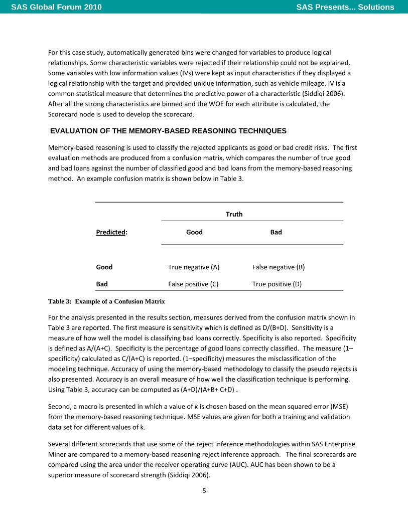
Memory-based reasoning is used to classify the rejected applicants as good or bad credit risks. The first

evaluation methods are produced from a confusion matrix, which compares the number of true good

and bad loans against the number of classified good and bad loans from the memory-based reasoning

method. An example confusion matrix is shown below in Table 3.

Truth

Predicted: Good Bad

Good True negative (A) False negative (B)

Bad False positive (C) True positive (D)

Table 3: Example of a Confusion Matrix

For the analysis presented in the results section, measures derived from the confusion matrix shown in

Table 3 are reported. The first measure is sensitivity which is defined as D/(B+D). Sensitivity is a

measure of how well the model is classifying bad loans correctly. Specificity is also reported. Specificity

is defined as A/(A+C). Specificity is the percentage of good loans correctly classified. The measure (1–

specificity) calculated as C/(A+C) is reported. (1–specificity) measures the misclassification of the

modeling technique. Accuracy of using the memory-based methodology to classify the pseudo rejects is

also presented. Accuracy is an overall measure of how well the classification technique is performing.

Using Table 3, accuracy can be computed as (A+D)/(A+B+ C+D) .

Second, a macro is presented in which a value of k is chosen based on the mean squared error (MSE)

from the memory-based reasoning technique. MSE values are given for both a training and validation

data set for different values of k.

Several different scorecards that use some of the reject inference methodologies within SAS Enterprise

Miner are compared to a memory-based reasoning reject inference approach. The final scorecards are

compared using the area under the receiver operating curve (AUC). AUC has been shown to be a

superior measure of scorecard strength (Siddiqi 2006).


6

RESULTS

The first set of result graphs are designed to decide which value of k is appropriate. Figures 2 through 4

show the sensitivity, specificity, and (1–specificity) values for different values of k. Figure 2 shows that as

k increases, the memory-based reasoning is doing a better job at classifying the bad loans correctly. This

result is due to the methodology behind the memory-based technique. As the neighborhood size

increases, more bad loans are being captured, thus increasing the chances of correctly classifying a bad

loan correctly.

The graph of specificity versus k shows an opposite pattern. As k increases, the percentage of good

loans that are correctly classified decreases. In terms of classifying good loans correctly, a smaller

neighborhood size is needed for this data set.

It is important for a risk manager to examine statistics such as sensitivity and specificity to obtain an

overall idea of how the reject inference model is classifying the good and bad loans. Typically, one of

the key goals in reject inference is to determine whether you are turning away any potential

creditworthy applicants. From a business perspective, the risk manager is trying to identify applicants

that should have been approved. Thus, the plot of (1–specificity) is very important.

Figure 4 displays the (1–specificity) measure for different values of k. The best (1–specificity) values are

obtained for higher values of k. The value (1–specificity) can be thought of as “turning money away.”

The quantity (1–specificity) represents the percentage of applicants that were really actually good loans,

but the model classified them as bad loans. If you want the best (1–specificity) rate, you should choose a

k value of 16 for this data.

Figure 5 displays the overall accuracy for different values of k using the memory-based methodology.

The best accuracy occurs when k is more than 13. Overall, for all values of k, accuracy is high.

Figure 2: Sensitivity versus k for the Pseudo Rejected Applicants Using Memory-Based Reasoning


7

Figure 3: Specificity versus k for the Pseudo Rejected Applicants Using Memory-Based Reasoning

Figure 4: (1–specificity) versus k for the Pseudo Rejected Applicants Using Memory-Based Reasoning

Figure 5: Accuracy rates versus k for the Pseudo Rejected Applicants Using Memory-Based Reasoning


8

Since different values of k were used, it would be interesting to see which value of k achieved the

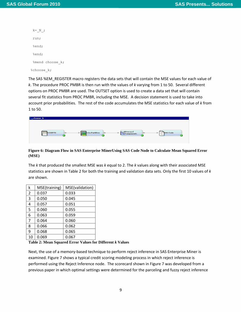
smallest MSE value for the memory-based methodology. Following is the %CHOOSE_k macro which was

written in a SAS code node within SAS Enterprise Miner. This macro creates a data set in which the MSE

values are accumulated for different values of k using the PMBR procedure. PROC PMBR is the

procedure that SAS uses within SAS Enterprise Miner to perform memory-based reasoning. Figure 6

displays the full diagram that was created in SAS Enterprise Miner. A Principal Component node must

be run prior to running PROC PMBR because one of the assumptions of memory-based reasoning is that

the input variables must be orthogonal and standardized (SAS Institute Inc. 2008).

%macro choose_k;

%do i=1 %to 50;

%em_register(key=f&i, type=data);

proc pmbr data=EMWS3.PRINCOMP_VALIDATE dmdbcat=&EM_USER_MBR_DMDB

outest = &&em_user_f&i

k = &i

epsilon = 0

method = SCAN

weighted;

target BAD_IND

decision decdata=&EM_USER_BAD_IND

decvars=

DECISION1

DECISION2

priorVar=DECPRIOR

;

run;

%if &i=1 %then %do;

data &EM_USER_MISC (keep= _VMSE_ );

set &&EM_USER_f&i ;

run;

%end;

%else %if &i ne 1 %then %do;

data &EM_USER_MISC (keep= _VMSE_ k );

set &EM_USER_MISC &&EM_USER_f&i;


9

k=_N_;

run;

%end;

%end;

%mend choose_k;

%choose_k;

The SAS %EM_REGISTER macro registers the data sets that will contain the MSE values for each value of

k. The procedure PROC PMBR is then run with the values of k varying from 1 to 50. Several different

options on PROC PMBR are used. The OUTSET option is used to create a data set that will contain

several fit statistics from PROC PMBR, including the MSE. A decision statement is used to take into

account prior probabilities. The rest of the code accumulates the MSE statistics for each value of k from

1 to 50.

Figure 6: Diagram Flow in SAS Enterprise MinerUsing SAS Code Node to Calculate Mean Squared Error

(MSE)

The k that produced the smallest MSE was k equal to 2. The k values along with their associated MSE

statistics are shown in Table 2 for both the training and validation data sets. Only the first 10 values of k

are shown.

k MSE(training) MSE(validation)

2 0.037 0.033

3 0.050 0.045

4 0.057 0.051

5 0.060 0.055

6 0.063 0.059

7 0.064 0.060

8 0.066 0.062

9 0.068 0.065

10 0.069 0.067 Table 2: Mean Squared Error Values for Different k Values

Next, the use of a memory-based technique to perform reject inference in SAS Enterprise Miner is

examined. Figure 7 shows a typical credit scoring modeling process in which reject inference is

performed using the Reject Inference node. The scorecard shown in Figure 7 was developed from a

previous paper in which optimal settings were determined for the parceling and fuzzy reject inference


10

techniques for this same data set (Anderson, Haller, and Siddiqi 2009). Those same settings for this

scorecard are used here to compare against the memory-based reject inference techniques.

Figure 7: Credit Scoring Process Using SAS Enterprise Miner

Figure 8 shows how this goal is achieved. First, the Score node is used to assign rejected applicants a

good/bad loan status based on the model created by the memory-based reasoning node. A SAS code

node is then used to create the augmented data set. The augmented data set contains the accepted

applicants (with their known good/bad loan status) and the rejected applicants with their classified

good/bad status coming from the MBR node. The SAS code node is also used to calculate the weight

variable for the rejected applicants. The weight variable is calculated in the same manner as it is

currently calculated using the reject inference node for each reject inference technique (Anderson,

Haller, and Siddiqi 2009).

After the augmented data set is created to remove the sample bias of building a scorecard solely on

accepted applicants, the credit scoring methodology is applied. The Interactive Grouping node is used

for grouping the interval level variables and to calculate the WOE values, and the Scorecard node is used

to create the scorecard. A Model Comparison node is used to obtain the AUC values. This process is

repeated for values of k from 2 to 16 in the memory-based reasoning node.

Figure 8: Using Memory-Based Reasoning as a Reject Inference Technique


11

First, the memory-based technique is compared to a reject inference parceling technique. Parceling

classifies rejected applicants in proportion to the expected bad rate at a particular credit score

(Anderson, Haller, and Siddiqi 2009). Using optimal settings for the parceling method, the final scorecard

shown in Figure 7 has an AUC value of 0.80. The AUC values for different values of k are shown in Table

3. When k reaches values of 15 or higher, the memory-based reject inference technique is

outperforming the parceling technique. Just as was shown in the plot of sensitivity, as k increases, the

methodology seems to be doing a better job at classifying. This phenomenon is due to the fact that as k

increases, the larger the region size is becoming for classification, hence increasing the chances of

correctly classifying an applicant.

k AUC Parceling-AUC

- 0.80

2 0.69

3 0.75

4 0.79

5 0.76

10 0.79

15 0.83

20 0.81

25 0.81

30 0.81 Table 3: Using Memory-Based Reasoning as a Reject Inference Technique for the Final Scorecard

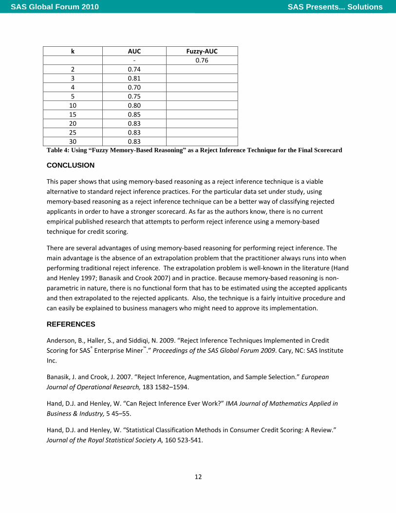
Table 4 shows the same type of results as Table 3, except now the fuzzy reject inference technique is

used to create the final scorecard shown in Figure 7(Anderson, Haller, and Siddiqi 2009). The fuzzy reject

inference technique assigns each rejected applicant into a “partial good” and a “partial bad”

classification. For each rejected applicant, two observations are generated: one observation has a good

loan status classification, and the other has a bad loan status classification (Anderson, Haller, and Siddiqi

2009).

A type of “fuzzy memory-based reasoning” is designed using the same type of flow that is shown in

Figure 8. In the SAS code node, two observations are generated for each rejected applicant. The weight

that is created for the rejected applicants was the same as using a fuzzy method except the predicted

probabilities that are in the weight formula are multiplied by the posterior probabilities from the MBR

node. Anderson, Haller, and Siddiqi 2009 give the details of how the weight is created for the fuzzy

method in the reject inference node.

As shown in Table 4, using optimal settings for the fuzzy method the final scorecard shown in Figure 7

has an AUC value of 0.76. When k reaches values of 10 or higher, the “fuzzy memory-based reasoning”

reject inference technique is outperforming the parceling technique.


12

k AUC Fuzzy-AUC

- 0.76

2 0.74

3 0.81

4 0.70

5 0.75

10 0.80

15 0.85

20 0.83

25 0.83

30 0.83 Table 4: Using “Fuzzy Memory-Based Reasoning” as a Reject Inference Technique for the Final Scorecard

CONCLUSION

This paper shows that using memory-based reasoning as a reject inference technique is a viable

alternative to standard reject inference practices. For the particular data set under study, using

memory-based reasoning as a reject inference technique can be a better way of classifying rejected

applicants in order to have a stronger scorecard. As far as the authors know, there is no current

empirical published research that attempts to perform reject inference using a memory-based

technique for credit scoring.

There are several advantages of using memory-based reasoning for performing reject inference. The

main advantage is the absence of an extrapolation problem that the practitioner always runs into when

performing traditional reject inference. The extrapolation problem is well-known in the literature (Hand

and Henley 1997; Banasik and Crook 2007) and in practice. Because memory-based reasoning is non-

parametric in nature, there is no functional form that has to be estimated using the accepted applicants

and then extrapolated to the rejected applicants. Also, the technique is a fairly intuitive procedure and

can easily be explained to business managers who might need to approve its implementation.

REFERENCES

Anderson, B., Haller, S., and Siddiqi, N. 2009. “Reject Inference Techniques Implemented in Credit

Scoring for SAS® Enterprise Miner™.” Proceedings of the SAS Global Forum 2009. Cary, NC: SAS Institute

Inc.

Banasik, J. and Crook, J. 2007. “Reject Inference, Augmentation, and Sample Selection.” European

Journal of Operational Research, 183 1582–1594.

Hand, D.J. and Henley, W. “Can Reject Inference Ever Work?” IMA Journal of Mathematics Applied in

Business & Industry, 5 45–55.

Hand, D.J. and Henley, W. “Statistical Classification Methods in Consumer Credit Scoring: A Review.”

Journal of the Royal Statistical Society A, 160 523-541.


13

SAS Institute Inc. (2008). “SAS Enterprise Miner and SAS Text Miner Procedures Reference for SAS 9.1.3

The PMBR Procedure (Book Excerpt).” Source downloaded from

<http://support.sas.com/documentation/onlinedoc/miner/emtmsas913/PMBR.pdf>

Siddiqi, Naeem. 2006. Credit Risk Scorecards: Developing and Implementing Intelligent Credit Scoring.

New York, NY: John Wiley & Sons.

Verstraeten, G. and Van den Poel, D. 2005. “The Impact of Sample Bias on Consumer Credit Scoring

Performance and Profitability.” Journal of the Operational Research Society, 56 981–992.

CONTACT INFORMATION

Your comments and questions are valued and encouraged. Contact the main author at:

Billie Anderson, Ph.D.

Research Statistician

SAS Institute Inc.

SAS Campus Dr.

Cary, NC 27513

Email: [email protected]


http://support.sas.com/documentation/onlinedoc/miner/emtmsas913/PMBR.pdf

mailto:[email protected]

Improving Credit Risk Scorecards

Documents

Transcript of Improving Credit Risk Scorecards