Improving Coverage Prediction for

Primary Multi-Transmitter Networks

Operating in the TV Whitespaces

Andreas Achtzehn, Janne Riihijarvi, Guilberth Martınez Vargas, Marina Petrova, Petri Mahonen

Institute for Networked Systems, RWTH Aachen University

Kackertstrasse 9, D-52072 Aachen, Germany

Email: {aac, jar, gma, mpe, pma}@inets.rwth-aachen.de

Abstract—Future wireless networks will be able to exploitunused spectrum whitespaces in the currently underutilizedterrestrial TV bands. In order to protect incumbent broadcastingsystems from extensive interference from whitespace devices,accurate signal power estimations are needed. Reliable and robustmodels for predicting the radio propagation in those bands arethus a key enabler of secondary operations. Depending on theirlevel of abstraction and the complexity of the environment, thesemodels can perform quite well, but they require a significantamount of auxiliary information and fine-tuning. Additionally,they usually consider transmitters in one frequency band tohave uncorrelated signals, an uncommon scenario in today’sdigital TV networks where the same geographical area is oftenserved by multiple towers that form a single-frequency network(SFN). Using data from a measurement campaign carried outin a mid-sized Central European city we assess the accuracy ofthree widely used propagation models in predicting TV signalstrengths for configurations of multiple high-power transmitters.We empirically show that the standard deviation of the estimationerror is up to 4 dB higher in a multi-transmitter scenarios withcorrelated signals than in the single-transmitter case. We putthe results in contrast to the prediction capabilities of a genericpropagation model that estimates pathloss coefficients and indi-vidual correction factors from measurements and combines themwith information on transmitter locations, power emissions andantenna patterns. Finally, we study the use of spatial statisticsbased techniques for directly estimating the coverage characteris-tics without relying on explicit transmitter information. We showthat with only a small subset of measurement locations accuracybeyond standard pathloss models can be achieved.

I. INTRODUCTION

Propagation models have for decades been used to predict

signal quality and improve performance of radio systems.

In future wireless networks, they will also be an essential

cornerstone for the peaceful coexistence of whitespace devices

with licensed primary operations. In order to estimate coverage

of primary systems and their robustness against interference

from secondary radio devices, these propagation models try

to estimate phenomena such as diffraction, scattering, and

reflection to make accurate predictions.

Many models are based on the observation that the received

signal is generally a mixture of delayed and attenuated copies

of the same transmitted waveform. Each of these signal

components is assumed to have traveled along a different

path to the receiver. Since the composition of paths and their

effects is specific to each scenario, pure physical models such

as the log-distance pathloss model are often augmented with

correction factors gathered from statistics derived in large-

scale measurement campaigns. Though these corrections may

improve their accuracy, propagation models remain to have a

non-negligible prediction error.

For the current generation of digital TV broadcasting net-

works, the imperfections of propagation models become even

more acute. In their often employed configuration as a single

frequency network (SFN), the same signal is emitted from

multiple sources and arrives at the receiver with an angle and

delay distribution that is considerably different from the single

transmitter case [1], [2]. Previously established knowledge on

the statistics of single-source signals used for traditional fine-

tuning of propagation models does not apply here anymore.

The resulting prediction error may lead to outage or severely

worsened performance once whitespace operations become

common in these bands. This raises the question of whether

new or modified prediction methods are required in order to

make more precise claims on the necessary protection of the

primary system against interference.

The peculiarities of the multi-transmitter scenario play until

now only a minor role in the literature on secondary operations

in TV bands. Given the advent of whitespace devices, we argue

that more research on this matter is urgently needed. We found

that in all currently proposed or enacted whitespace ruling,

only rudimentary assumptions were made on the configuration

of the primary TV system. For all cases, a simple summation

of signal powers as predicted for the individual TV transmitters

has been deemed sufficient. Following our argument above we

expect that this approach may result in even higher prediction

errors, not only because each signal contribution is afflicted

with an individual prediction error, but also due to the signal

cancellation and amplifications effects of highly correlated

signals that may manifest here.

In order to quantify the prediction errors in the multi-

transmitter scenario that may arise in propagation modeling for

TV whitespaces, we study the complex case of a real urban

environment. We initially assess the propagation variability

2012 9th Annual IEEE Communications Society Conference on Sensor, Mesh and Ad Hoc Communications and Networks(SECON)

978-1-4673-1905-8/12/$31.00 ©2012 IEEE 547

from a measurement campaign that was carried out for three

different tower configurations in a Central European city. In

the following we investigate whether traditional propagation

models may be improved to better capture multi-transmitter

scenarios by incorporating the results of a limited number

of measurements. We explore two complementary methods in

this paper that either try to improve the parametric fit of an

existing propagation model or build upon spatial statistics to

estimate the surrounding radio environment. The results of

this paper are indicative for the requirement to build more

sophisticated coverage prediction models for TV networks that

need to incorporate configuration-specific features to derive the

protection requirements for whitespace devices.

This paper is organized as follows: In Section II we present

a concise overview of related work on propagation modeling.

To build a practical foundation for our work, we report

in Section III on the results of a measurement campaign

that we have carried out in a mid-sized city. Section IV

quantifies the estimation errors of current propagation models

for the studied scenario. Results from our efforts to improve

the predictive capabilities of an existing model with limited

measurements are presented in Section V. An alternative

approach to measurement-based propagation prediction that

employs spatial statistics is discussed in Section VI. Section

VII concludes the paper.

II. RELATED WORK

The switch-over from analogue to digital systems for TV

broadcasting, accompanied by an exponential growth in wire-

less data consumption has raised interest in allowing sec-

ondary wireless operations in the TV bands. The amount of

whitespace that will be freed in accordance with regulatory

legislation on interference has been initially acquired e.g. for

the U.S. by Harrison et al. [3] and for Central Europe by

van de Beek et al. [4], and has subsequently been studied for

deployment prospects of secondary networks, e.g. in [5].

With the emergence of the digital broadcasting standards,

new design-induced constraints of single frequency networks

have started to be of practical concern. Common potential

pitfalls have been identified, e.g. by Mattsson [6]. Tang et al.

[2] have carried out empirical tests with a deployment of two

synchronized transmitters and found that a tapped delay line

(TDL) approach for modeling the signal is a feasible approach

for their controlled scenario in a rural environment.

The specific propagation of multi-transmitter TV signals

in urban environments has been the subject of works by

Angueira et al. [1]. They have carried out measurements for

a three-tower scenario in Madrid, Spain and have derived

a technology-specific mapping between carrier-to-noise ratio

and bit-error rate for this case.

Fitting measurement data to assumptions on RF propagation

has been conducted for many different terrains, climates and

environments and had led to the derivation of such widely

used models as the Okumura-Hata model [7], [8] or the ITU

model P.1546-3 [9]. The amount of literature in this area is

vast, therefore we can only refer to some good review text

450mmap source: openstreetmap.org

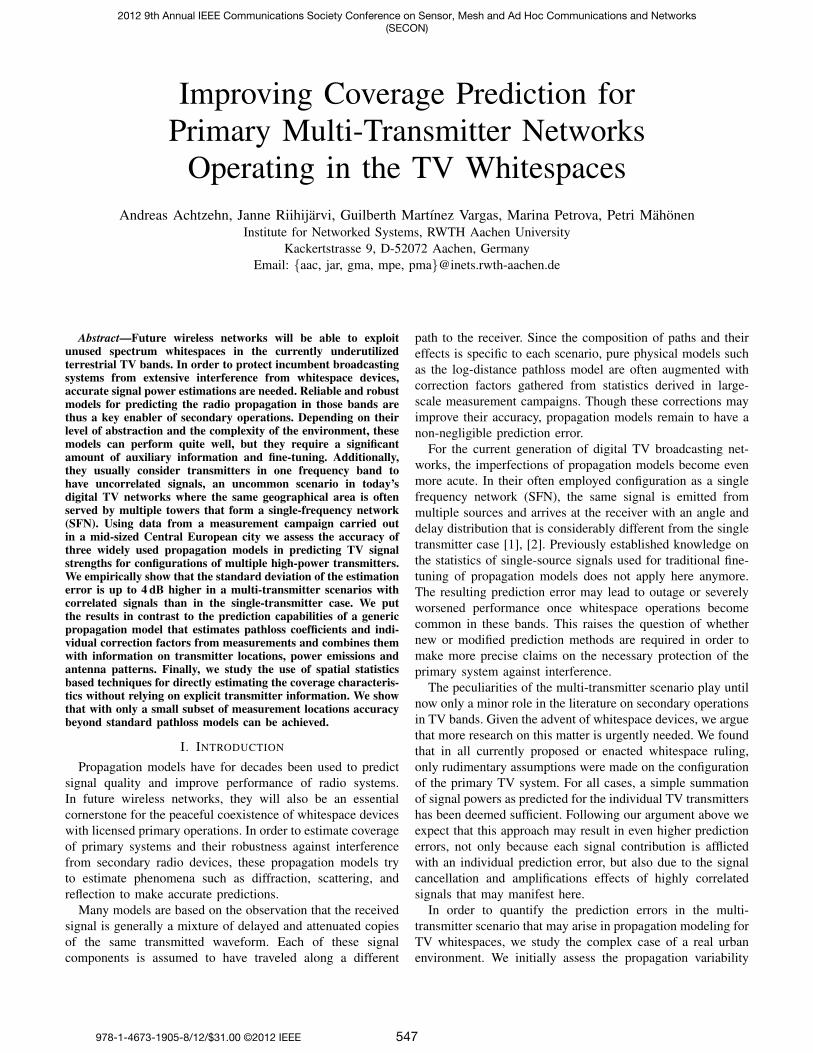
Fig. 1. Measurement locations in Aachen, Germany.

books, e.g. [10], [11]. The specific strengths and weaknesses of

models are often of interest when an application choice needs

to be made. Lately, comparison studies have been conducted

e.g. by Phillips et al. [12], who, like us, conduct parameter

fitting for the urban scenario. While their work is focusing

on data gathered for a magnitude of low-power transmitters

operating within the study region, we focus in our work

on holistically capturing the propagation effects for a small

number of high-power transmitters outside the region.

TABLE IMEASUREMENT EQUIPMENT AND CONFIGURATION.

Spectrum analyzer Rohde & Schwarz FSL6

Displayed average noise −162 dBm/Hz

Preamplifier 20 dB

Resolution bandwidth 300 kHz

Sweep points 251 per sweepSweep time 420ms per sweepNumber of sweepsper location

1000

Center frequency Sweep 1: 514MHz

Sweep 2: 586MHz

Frequency span 75.3MHz

Detector RMSRepeatability 0.05 dB/99%

Antenna Aaronia BicoLOG 30100

Form factor BiconicalAntenna height 1.8meters

Gain (typ.) 1 dBi

Mechanical tilting precision ±5◦

Other components

Cable losses (typ.) 0.3 dB @ 500MHz

Reported channel noise floor(typ.)

−91.95 dBm

(±0.91 dB)

548

Belgium

Nether-

lands

Germany

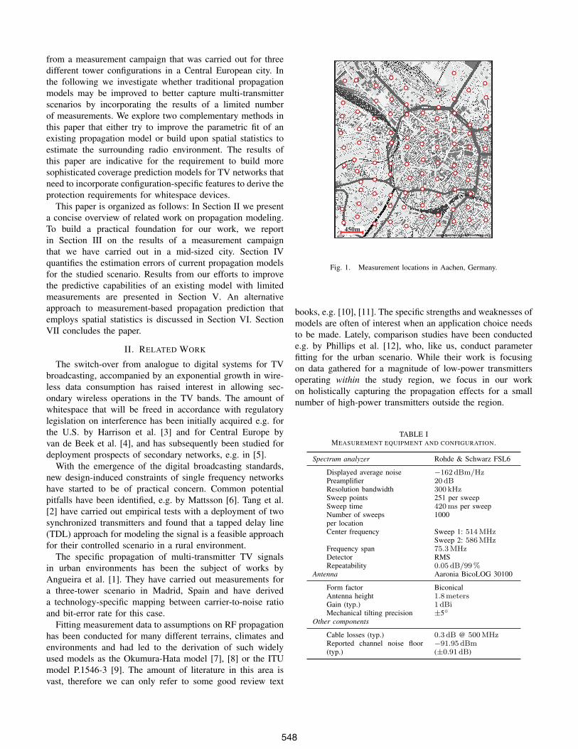
Fig. 2. Observable TV transmitters with the study region shown as the redsquare.

III. MEASUREMENT CAMPAIGN

In order to determine the combined signal strength received

from multiple TV transmitters, a measurement campaign was

carried out in Aachen, a mid-sized German town located at

the border to the Netherlands and Belgium. Like many other

Central European cities, Aachen exhibits a circular cultivation,

with a commercial area in the center, nestled by two ring roads

that separate it from residential and industrial areas. Aachen

is surrounded by a natural elevation partially shadowing it

against outside radio emissions. Given its population and

layout, it is regarded to be a typical urban scenario in this

area.

During the campaign, measurements were carried out at 96

roughly equidistant locations in a 2.5 km×3 km regular grid,

shown as red circles in the Figure 1. The distance between

grid points was chosen to fit the 3-arc second resolution of

terrain data provided through the Shuttle Radar Topography

Mission (SRTM) [13] required later. We manually selected

measurement locations in a way that they do not follow each

other along the same line-of-sight path of any of the measured

transmitters. Furthermore, to minimize the potential waveg-

uiding effects along streets observed in earlier measurement

campaigns [14], measurement points do not have a line of

sight between them.

A test setup with the key features listed in Table I was

built to specifically meet the requirements for measuring TV

signals with the peculiarities of the scenario at hand. Besides

a high-precision spectrum analyzer with low residual noise

floor, a mast-mounted antenna construction was built to simul-

taneously capture power emissions of all radio sources. Due

to the predominance of vertically-polarized TV transmitters

in the area, the antenna was mounted perpendicularly and

mechanically aligned to the vertical plane at each location.

Samples were created repeatedly with the smallest possible

resolution of the hardware to average over fast-fading, modu-

lation effects and the noise floor of the device, and combined

to create channel power estimations.

A. Radio Environment

Within the selected frequency range, the study region is

served by three multi-transmitter setups shown in Figure 2

and furthermore denoted by the TV broadcasting-specific

term as Single Frequency Networks (SFNs). Information on

these SFNs including tower locations, transmit powers and

antenna patterns is publicly available through the national

regulator [15] and has been used as a reference for the our

assessment. Resulting statistics of a selection of channels are

listed in Table II. The Aachen SFN is the closest one and

consists of two towers, located South-West and North-East

of the study region, respectively. The smaller Aachen tower

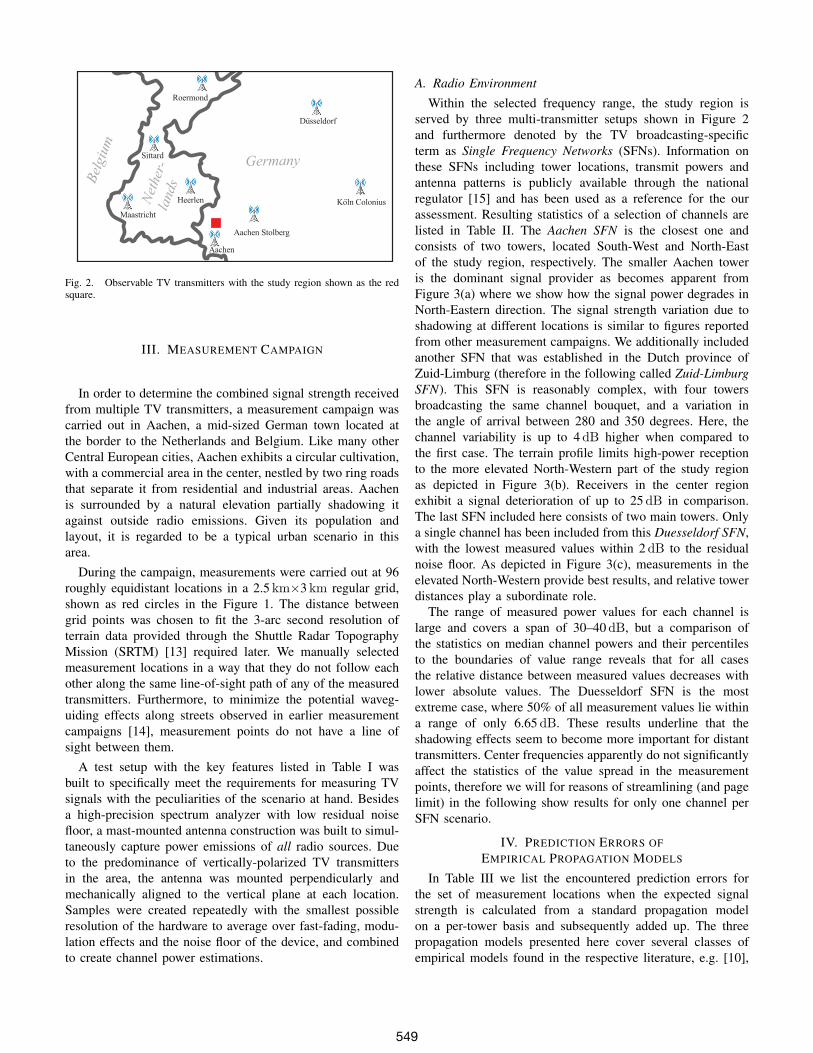
is the dominant signal provider as becomes apparent from

Figure 3(a) where we show how the signal power degrades in

North-Eastern direction. The signal strength variation due to

shadowing at different locations is similar to figures reported

from other measurement campaigns. We additionally included

another SFN that was established in the Dutch province of

Zuid-Limburg (therefore in the following called Zuid-Limburg

SFN). This SFN is reasonably complex, with four towers

broadcasting the same channel bouquet, and a variation in

the angle of arrival between 280 and 350 degrees. Here, the

channel variability is up to 4dB higher when compared to

the first case. The terrain profile limits high-power reception

to the more elevated North-Western part of the study region

as depicted in Figure 3(b). Receivers in the center region

exhibit a signal deterioration of up to 25dB in comparison.

The last SFN included here consists of two main towers. Only

a single channel has been included from this Duesseldorf SFN,

with the lowest measured values within 2dB to the residual

noise floor. As depicted in Figure 3(c), measurements in the

elevated North-Western provide best results, and relative tower

distances play a subordinate role.

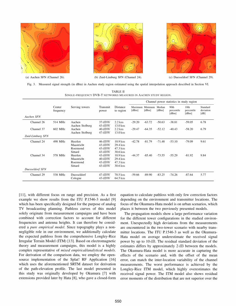
The range of measured power values for each channel is

large and covers a span of 30–40dB, but a comparison of

the statistics on median channel powers and their percentiles

to the boundaries of value range reveals that for all cases

the relative distance between measured values decreases with

lower absolute values. The Duesseldorf SFN is the most

extreme case, where 50% of all measurement values lie within

a range of only 6.65dB. These results underline that the

shadowing effects seem to become more important for distant

transmitters. Center frequencies apparently do not significantly

affect the statistics of the value spread in the measurement

points, therefore we will for reasons of streamlining (and page

limit) in the following show results for only one channel per

SFN scenario.

IV. PREDICTION ERRORS OF

EMPIRICAL PROPAGATION MODELS

In Table III we list the encountered prediction errors for

the set of measurement locations when the expected signal

strength is calculated from a standard propagation model

on a per-tower basis and subsequently added up. The three

propagation models presented here cover several classes of

empirical models found in the respective literature, e.g. [10],

549

(a) Aachen SFN (Channel 26). (b) Zuid-Limburg SFN (Channel 24). (c) Duesseldorf SFN (Channel 29).

Fig. 3. Measured signal strength (in dBm) in Aachen study region estimated using the spatial interpolation approach described in Section VI.

TABLE IISINGLE-FREQUENCY DVB-T NETWORKS MEASURED IN AACHEN STUDY REGION.

Channel power statistics in study region

Centerfrequency

Serving towers Transmitpower

Distanceto region

Maximum

[dBm]

Minimum

[dBm]

Median

[dBm]

90th

percentile

[dBm]

10th

percentile

[dBm]

Standard

deviation

[dB]

Aachen SFN

Channel 26 514 MHz Aachen 37 dBW 2.2 km -29.20 -63.72 -50.63 -38.81 -59.05 6.78Aachen Stolberg 43 dBW 13.0 km

Channel 37 602 MHz Aachen 40 dBW 2.2 km -29.47 -64.35 -52.12 -40.43 -58.20 6.79Aachen Stolberg 47 dBW 13.0 km

Zuid-Limburg SFN

Channel 24 498 MHz Heerlen 46 dBW 10.9 km -42.78 -81.79 -71.48 -53.10 -79.09 9.61Maastricht 43 dBW 29.4 kmRoermond 43 dBW 47.3 kmSittard 43 dBW 30.6 km

Channel 34 578 MHz Heerlen 43 dBW 10.9 km -44.37 -85.40 -73.55 -55.29 -81.92 9.84Maastricht 40 dBW 29.4 kmRoermond 43 dBW 47.3 kmSittard 43 dBW 30.6 km

Duesseldorf SFN

Channel 29 538 MHz Duesseldorf 47 dBW 70.5 km -59.66 -89.90 -83.25 -74.26 -87.64 5.77Cologne 43 dBW 64.5 km

[11], with different focus on range and precision. As a first

example we show results from the ITU P.1546-3 model [9]

which has been specifically designed for the purpose of analog

TV broadcasting planning. Pathloss curves of this model

solely originate from measurement campaigns and have been

combined with correction factors to account for different

frequencies and antenna heights. It can therefore be consid-

ered a pure empirical model. Since topography plays a non-

negligible role in our environment, we additionally calculate

the expected pathloss from the comprehensive Longley-Rice

Irregular Terrain Model (ITM) [13]. Based on electromagnetic

theory and measurement campaigns, this model is a highly

complex representative of mixed empirical/analytical models.

For derivation of the comparison data, we employ the open-

source implementation of the Splat! RF Application [16]

which uses the aforementioned SRTM dataset for derivation

of the path-elevation profile. The last model presented in

this study was originally developed by Okumura [7] with

extensions provided later by Hata [8], who gave a closed-form

equation to calculate pathloss with only few correction factors

depending on the environment and transmitter locations. The

focus of the Okumura-Hata model is on urban scenarios, which

places it between the two previously presented models.

The propagation models show a large performance variation

for the different tower configurations in the studied environ-

ment. Unexpectedly high deviations from the measurements

are encountered in the two-tower scenario with nearby trans-

mitter locations. The ITU P.1546-3 as well as the Okumura-

Hata model on average underestimate the received signal

power by up to 10dB. The residual standard deviation of the

estimates differs by approximately 2dB between the models.

The Okumura-Hata model is more accurate in capturing the

effects of the scenario and, with the offset of the mean

error, can match the inter-location variability of the channel

measurements. The worst performance is achieved by the

Longley-Rice ITM model, which highly overestimates the

received signal power. The ITM model also shows residual

error moments of the distribution that are not superior over the

550

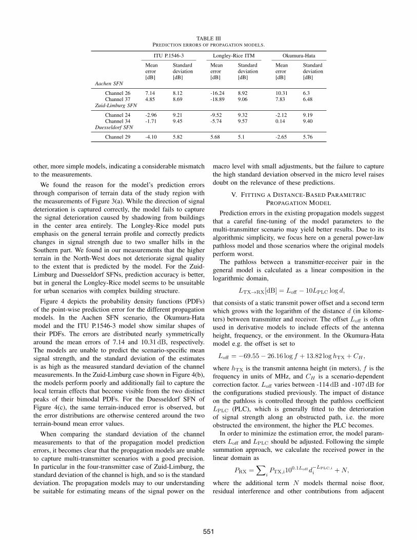
TABLE IIIPREDICTION ERRORS OF PROPAGATION MODELS.

ITU P.1546-3 Longley-Rice ITM Okumura-Hata

Meanerror[dB]

Standarddeviation[dB]

Meanerror[dB]

Standarddeviation[dB]

Meanerror[dB]

Standarddeviation[dB]

Aachen SFN

Channel 26 7.14 8.12 -16.24 8.92 10.31 6.3Channel 37 4.85 8.69 -18.89 9.06 7.83 6.48

Zuid-Limburg SFN

Channel 24 -2.96 9.21 -9.52 9.32 -2.12 9.19Channel 34 -1.71 9.45 -5.74 9.57 0.14 9.40

Duesseldorf SFN

Channel 29 -4.10 5.82 5.68 5.1 -2.65 5.76

other, more simple models, indicating a considerable mismatch

to the measurements.

We found the reason for the model’s prediction errors

through comparison of terrain data of the study region with

the measurements of Figure 3(a). While the direction of signal

deterioration is captured correctly, the model fails to capture

the signal deterioration caused by shadowing from buildings

in the center area entirely. The Longley-Rice model puts

emphasis on the general terrain profile and correctly predicts

changes in signal strength due to two smaller hills in the

Southern part. We found in our measurements that the higher

terrain in the North-West does not deteriorate signal quality

to the extent that is predicted by the model. For the Zuid-

Limburg and Duesseldorf SFNs, prediction accuracy is better,

but in general the Longley-Rice model seems to be unsuitable

for urban scenarios with complex building structure.

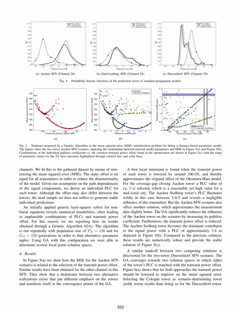
Figure 4 depicts the probability density functions (PDFs)

of the point-wise prediction error for the different propagation

models. In the Aachen SFN scenario, the Okumura-Hata

model and the ITU P.1546-3 model show similar shapes of

their PDFs. The errors are distributed nearly symmetrically

around the mean errors of 7.14 and 10.31dB, respectively.The models are unable to predict the scenario-specific mean

signal strength, and the standard deviation of the estimates

is as high as the measured standard deviation of the channel

measurements. In the Zuid-Limburg case shown in Figure 4(b),

the models perform poorly and additionally fail to capture the

local terrain effects that become visible from the two distinct

peaks of their bimodal PDFs. For the Duesseldorf SFN of

Figure 4(c), the same terrain-induced error is observed, but

the error distributions are otherwise centered around the two

terrain-bound mean error values.

When comparing the standard deviation of the channel

measurements to that of the propagation model prediction

errors, it becomes clear that the propagation models are unable

to capture multi-transmitter scenarios with a good precision.

In particular in the four-transmitter case of Zuid-Limburg, the

standard deviation of the channel is high, and so is the standard

deviation. The propagation models may to our understanding

be suitable for estimating means of the signal power on the

macro level with small adjustments, but the failure to capture

the high standard deviation observed in the micro level raises

doubt on the relevance of these predictions.

V. FITTING A DISTANCE-BASED PARAMETRIC

PROPAGATION MODEL

Prediction errors in the existing propagation models suggest

that a careful fine-tuning of the model parameters to the

multi-transmitter scenario may yield better results. Due to its

algorithmic simplicity, we focus here on a general power-law

pathloss model and those scenarios where the original models

perform worst.

The pathloss between a transmitter-receiver pair in the

general model is calculated as a linear composition in the

logarithmic domain,

LTX→RX[dB] = Loff − 10LPLC log d,

that consists of a static transmit power offset and a second term

which grows with the logarithm of the distance d (in kilome-

ters) between transmitter and receiver. The offset Loff is often

used in derivative models to include effects of the antenna

height, frequency, or the environment. In the Okumura-Hata

model e.g. the offset is set to

Loff = −69.55− 26.16 log f + 13.82 log hTX + CH ,

where hTX is the transmit antenna height (in meters), f is the

frequency in units of MHz, and CH is a scenario-dependent

correction factor. Loff varies between -114dB and -107dB for

the configurations studied previously. The impact of distance

on the pathloss is controlled through the pathloss coefficient

LPLC (PLC), which is generally fitted to the deterioration

of signal strength along an obstructed path, i.e. the more

obstructed the environment, the higher the PLC becomes.

In order to minimize the estimation error, the model param-

eters Loff and LPLC should be adjusted. Following the simple

summation approach, we calculate the received power in the

linear domain as

PRX =∑

iPTX,i10

0.1Loffd−LPLC,i

i +N,

where the additional term N models thermal noise floor,

residual interference and other contributions from adjacent

551

−30 −20 −10 0 10 20 300

0.01

0.02

0.03

0.04

0.05

0.06

0.07

0.08

0.09

0.1

0.11

Prediction error [dB]

PD

F

ITU P.1546−3Longley-RiceOkumura-Hata

(a) Aachen SFN (Channel 26).

−30 −20 −10 0 10 20 300

0.01

0.02

0.03

0.04

0.05

0.06

0.07

0.08

0.09

0.1

0.11

Prediction error [dB]

PD

F

ITU P.1546−3Longley-RiceOkumura-Hata

(b) Zuid-Limburg SFN (Channel 24).

−30 −20 −10 0 10 20 300

0.01

0.02

0.03

0.04

0.05

0.06

0.07

0.08

0.09

0.1

0.11

Prediction error [dB]

PD

F

ITU P.1546−3Longley-RiceOkumura-Hata

(c) Duesseldorf SFN (Channel 29).

Fig. 4. Probability density functions of the prediction errors of standard propagation models.

−100 −95 −90 −85384

386

388

390

392

394

396

398

Transmit power o!set [dB]

Me

an

Sq

ua

red

Err

or

(MS

E)

(a)

384

386

388

390

392

394

396

398M

ea

n S

qu

are

d E

rro

r (M

SE

)

2.5 3 3.5 4 4.5 5 5.5 6Pathloss coe!cient

AachenAachen Stolberg

(b)

−98 −96 −94 −92 −90 −883

3.5

4

4.5

5

5.5

Transmit power o!set [dB]

Pa

thlo

ss c

oe

"ci

en

t

AachenAachen Stolberg

(c)

Fig. 5. Solutions proposed by a Genetic Algorithm to the mean squared error (MSE) minimization problem for fitting a distance-based parametric model.The figures show the two-tower Aachen SFN scenario, depicting the relationship between selected model parameters and MSE in Figure 5(a) and Figure 5(b).Combinations of the individual pathloss coefficients vs. the common transmit power offset found in the optimization are shown in Figure 5(c) with the rangeof parameter values for the 5% best outcomes highlighted through colored bars and solid lines.

channels. We fit this to the gathered dataset by means of min-

imizing the mean squared error (MSE). The static offset is set

equal for all transmitters in order to reduce the dimensionality

of the model. Given our assumption on the path dependencies

of the signal components, we derive an individual PLC for

each tower. Although the offset may also differ between the

towers, the used sample set does not suffice to generate stable

individual predictions.

An initially applied generic least-squares solver for non-

linear equations reveals numerical instabilities, often leading

to implausible combinations of PLCs and transmit power

offset. For this reason, we are reporting here on results

obtained through a Genetic Algorithm (GA). The algorithm

is run repeatedly with population size of PN = 120 and for

GN = 150 generations in order to find alternative parameter

tuples. Using GA with this configuration we were able to

determine several focal point solution spaces.

A. Results

In Figure 5(a) we show how the MSE for the Aachen SFN

scenario is related to the selection of the transmit power offset.

Similar results have been obtained for the other channel in this

SFN. They show that a dichotomy between two alternative

realizations exists that put different emphasis on the towers

and manifests itself in the convergence points of the GA.

A first local minimum is found when the transmit power

of each tower is lowered by around 100dB, and thereby

approximates the original offset of the Okumura-Hata model.

For the coverage-gap closing Aachen tower a PLC value of

ca. 3 is selected, which is a reasonable yet high value for a

mid-sized city. The Aachen Stolberg tower’s PLC fluctuates

wildly in this case between 3–6.5 and reveals a negligible

influence of this transmitter. But the Aachen SFN scenario also

offers another solution, which approximates the measurement

data slightly better. The GA significantly reduces the influence

of the Aachen tower on the scenario by increasing its pathloss

coefficient. Furthermore, the transmit power offset is reduced.

The Aachen Stolberg tower becomes the dominant contributor

to the signal power with a PLC of approximately 3.4 as

depicted in Figure 5(b). Compared to the previous solution,

these results are numerically robust and provide the stable

solution of Figure 5(c).

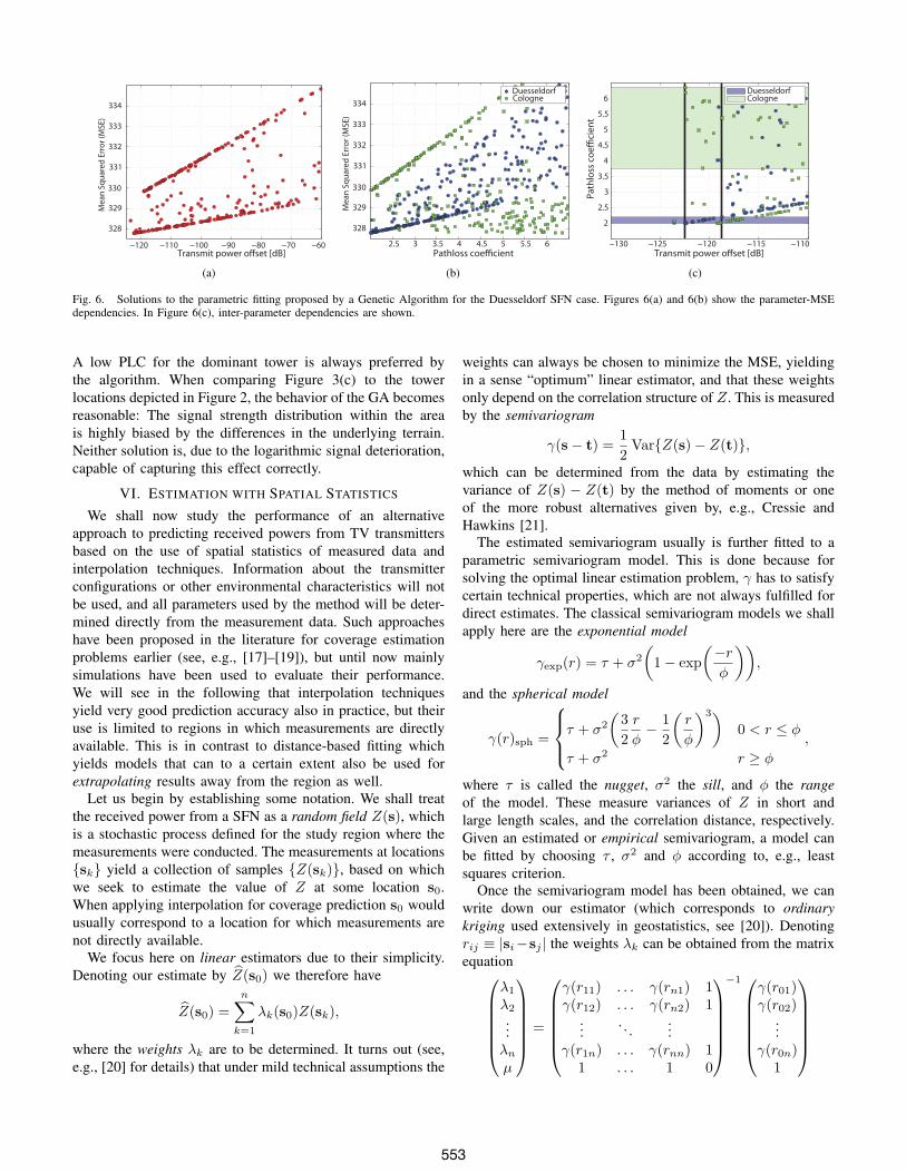
A similar tradeoff between two competing solutions is

discovered for the two-tower Duesseldorf SFN scenario. The

GA converges towards two solution spaces in which either

of the tower’s PLC is matched with the transmit power offset.

Figure 6(a) shows that for both approaches the transmit power

should be lowered to improve on the mean squared error.

Selecting the Cologne tower as scenario-determining tower

yields worse results than doing so for the Duesseldorf tower.

552

−120 −110 −100 −90 −80 −70 −60

328

329

330

331

332

333

334

Transmit power o!set [dB]

Me

an

Sq

ua

red

Err

or

(MS

E)

(a)

2.5 3 3.5 4 4.5 5 5.5 6

DuesseldorfCologne

328

329

330

331

332

333

334

Pathloss coe!cient

Me

an

Sq

ua

red

Err

or

(MS

E)

(b)

−130 −125 −120 −115 −110

2

2.5

3

3.5

4

4.5

5

5.5

6

Transmit power o!set [dB]

Pa

thlo

ss c

oe

"ci

en

t

DuesseldorfCologne

(c)

Fig. 6. Solutions to the parametric fitting proposed by a Genetic Algorithm for the Duesseldorf SFN case. Figures 6(a) and 6(b) show the parameter-MSEdependencies. In Figure 6(c), inter-parameter dependencies are shown.

A low PLC for the dominant tower is always preferred by

the algorithm. When comparing Figure 3(c) to the tower

locations depicted in Figure 2, the behavior of the GA becomes

reasonable: The signal strength distribution within the area

is highly biased by the differences in the underlying terrain.

Neither solution is, due to the logarithmic signal deterioration,

capable of capturing this effect correctly.

VI. ESTIMATION WITH SPATIAL STATISTICS

We shall now study the performance of an alternative

approach to predicting received powers from TV transmitters

based on the use of spatial statistics of measured data and

interpolation techniques. Information about the transmitter

configurations or other environmental characteristics will not

be used, and all parameters used by the method will be deter-

mined directly from the measurement data. Such approaches

have been proposed in the literature for coverage estimation

problems earlier (see, e.g., [17]–[19]), but until now mainly

simulations have been used to evaluate their performance.

We will see in the following that interpolation techniques

yield very good prediction accuracy also in practice, but their

use is limited to regions in which measurements are directly

available. This is in contrast to distance-based fitting which

yields models that can to a certain extent also be used for

extrapolating results away from the region as well.

Let us begin by establishing some notation. We shall treat

the received power from a SFN as a random field Z(s), whichis a stochastic process defined for the study region where the

measurements were conducted. The measurements at locations

{sk} yield a collection of samples {Z(sk)}, based on which

we seek to estimate the value of Z at some location s0.

When applying interpolation for coverage prediction s0 would

usually correspond to a location for which measurements are

not directly available.

We focus here on linear estimators due to their simplicity.

Denoting our estimate by Z(s0) we therefore have

Z(s0) =n∑

k=1

λk(s0)Z(sk),

where the weights λk are to be determined. It turns out (see,

e.g., [20] for details) that under mild technical assumptions the

weights can always be chosen to minimize the MSE, yielding

in a sense “optimum” linear estimator, and that these weights

only depend on the correlation structure of Z. This is measured

by the semivariogram

γ(s− t) =1

2Var{Z(s)− Z(t)},

which can be determined from the data by estimating the

variance of Z(s) − Z(t) by the method of moments or one

of the more robust alternatives given by, e.g., Cressie and

Hawkins [21].

The estimated semivariogram usually is further fitted to a

parametric semivariogram model. This is done because for

solving the optimal linear estimation problem, γ has to satisfy

certain technical properties, which are not always fulfilled for

direct estimates. The classical semivariogram models we shall

apply here are the exponential model

γexp(r) = τ + σ2

(1− exp

(−r

φ

)),

and the spherical model

γ(r)sph =

τ + σ2

(3

2

r

φ−

1

2

(r

φ

)3)0 < r ≤ φ

τ + σ2 r ≥ φ

,

where τ is called the nugget, σ2 the sill, and φ the range

of the model. These measure variances of Z in short and

large length scales, and the correlation distance, respectively.

Given an estimated or empirical semivariogram, a model can

be fitted by choosing τ , σ2 and φ according to, e.g., least

squares criterion.

Once the semivariogram model has been obtained, we can

write down our estimator (which corresponds to ordinary

kriging used extensively in geostatistics, see [20]). Denoting

rij ≡ |si−sj | the weights λk can be obtained from the matrix

equation

λ1

λ2

...

λn

µ

=

γ(r11) . . . γ(rn1) 1γ(r12) . . . γ(rn2) 1

.... . .

...

γ(r1n) . . . γ(rnn) 11 . . . 1 0

−1

γ(r01)γ(r02)

...

γ(r0n)1

553

0 500 1000 1500 2000 2500

0

10

20

30

40

Distance [m]

Sem

ivar

ian

ce

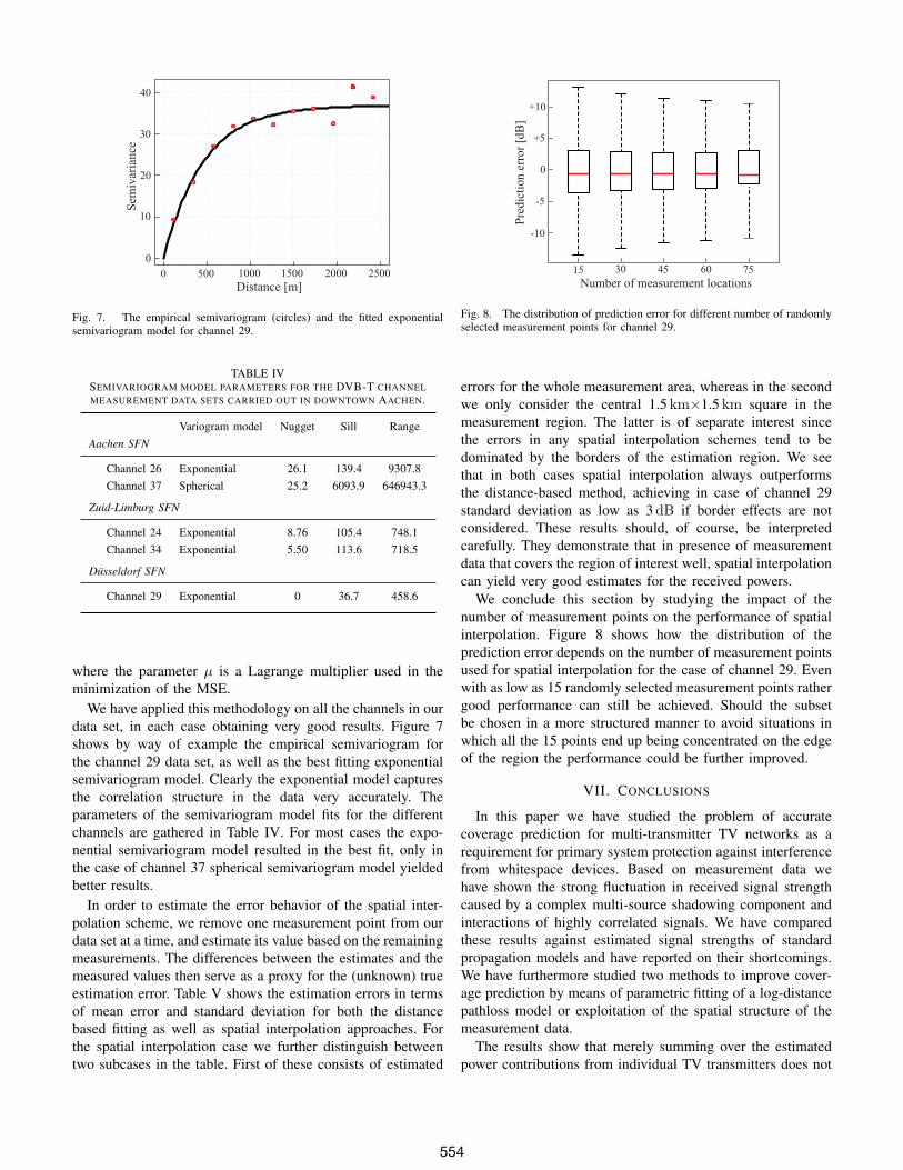
Fig. 7. The empirical semivariogram (circles) and the fitted exponentialsemivariogram model for channel 29.

TABLE IVSEMIVARIOGRAM MODEL PARAMETERS FOR THE DVB-T CHANNEL

MEASUREMENT DATA SETS CARRIED OUT IN DOWNTOWN AACHEN.

Variogram model Nugget Sill Range

Aachen SFN

Channel 26 Exponential 26.1 139.4 9307.8

Channel 37 Spherical 25.2 6093.9 646943.3

Zuid-Limburg SFN

Channel 24 Exponential 8.76 105.4 748.1

Channel 34 Exponential 5.50 113.6 718.5

Dusseldorf SFN

Channel 29 Exponential 0 36.7 458.6

where the parameter µ is a Lagrange multiplier used in the

minimization of the MSE.

We have applied this methodology on all the channels in our

data set, in each case obtaining very good results. Figure 7

shows by way of example the empirical semivariogram for

the channel 29 data set, as well as the best fitting exponential

semivariogram model. Clearly the exponential model captures

the correlation structure in the data very accurately. The

parameters of the semivariogram model fits for the different

channels are gathered in Table IV. For most cases the expo-

nential semivariogram model resulted in the best fit, only in

the case of channel 37 spherical semivariogram model yielded

better results.

In order to estimate the error behavior of the spatial inter-

polation scheme, we remove one measurement point from our

data set at a time, and estimate its value based on the remaining

measurements. The differences between the estimates and the

measured values then serve as a proxy for the (unknown) true

estimation error. Table V shows the estimation errors in terms

of mean error and standard deviation for both the distance

based fitting as well as spatial interpolation approaches. For

the spatial interpolation case we further distinguish between

two subcases in the table. First of these consists of estimated

15 30 45 60 75

-10

-5

0

+5

+10

Number of measurement locations

Pre

dic

tio

n e

rro

r [d

B]

Fig. 8. The distribution of prediction error for different number of randomlyselected measurement points for channel 29.

errors for the whole measurement area, whereas in the second

we only consider the central 1.5 km×1.5 km square in the

measurement region. The latter is of separate interest since

the errors in any spatial interpolation schemes tend to be

dominated by the borders of the estimation region. We see

that in both cases spatial interpolation always outperforms

the distance-based method, achieving in case of channel 29

standard deviation as low as 3dB if border effects are not

considered. These results should, of course, be interpreted

carefully. They demonstrate that in presence of measurement

data that covers the region of interest well, spatial interpolation

can yield very good estimates for the received powers.

We conclude this section by studying the impact of the

number of measurement points on the performance of spatial

interpolation. Figure 8 shows how the distribution of the

prediction error depends on the number of measurement points

used for spatial interpolation for the case of channel 29. Even

with as low as 15 randomly selected measurement points rather

good performance can still be achieved. Should the subset

be chosen in a more structured manner to avoid situations in

which all the 15 points end up being concentrated on the edge

of the region the performance could be further improved.

VII. CONCLUSIONS

In this paper we have studied the problem of accurate

coverage prediction for multi-transmitter TV networks as a

requirement for primary system protection against interference

from whitespace devices. Based on measurement data we

have shown the strong fluctuation in received signal strength

caused by a complex multi-source shadowing component and

interactions of highly correlated signals. We have compared

these results against estimated signal strengths of standard

propagation models and have reported on their shortcomings.

We have furthermore studied two methods to improve cover-

age prediction by means of parametric fitting of a log-distance

pathloss model or exploitation of the spatial structure of the

measurement data.

The results show that merely summing over the estimated

power contributions from individual TV transmitters does not

554

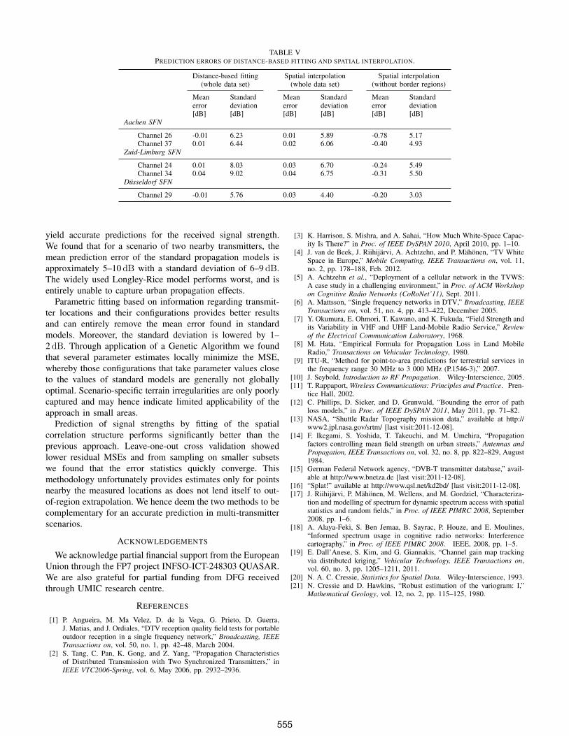
TABLE VPREDICTION ERRORS OF DISTANCE-BASED FITTING AND SPATIAL INTERPOLATION.

Distance-based fitting Spatial interpolation Spatial interpolation(whole data set) (whole data set) (without border regions)

Meanerror[dB]

Standarddeviation[dB]

Meanerror[dB]

Standarddeviation[dB]

Meanerror[dB]

Standarddeviation[dB]

Aachen SFN

Channel 26 -0.01 6.23 0.01 5.89 -0.78 5.17Channel 37 0.01 6.44 0.02 6.06 -0.40 4.93

Zuid-Limburg SFN

Channel 24 0.01 8.03 0.03 6.70 -0.24 5.49Channel 34 0.04 9.02 0.04 6.75 -0.31 5.50

Dusseldorf SFN

Channel 29 -0.01 5.76 0.03 4.40 -0.20 3.03

yield accurate predictions for the received signal strength.

We found that for a scenario of two nearby transmitters, the

mean prediction error of the standard propagation models is

approximately 5–10dB with a standard deviation of 6–9dB.The widely used Longley-Rice model performs worst, and is

entirely unable to capture urban propagation effects.

Parametric fitting based on information regarding transmit-

ter locations and their configurations provides better results

and can entirely remove the mean error found in standard

models. Moreover, the standard deviation is lowered by 1–

2dB. Through application of a Genetic Algorithm we found

that several parameter estimates locally minimize the MSE,

whereby those configurations that take parameter values close

to the values of standard models are generally not globally

optimal. Scenario-specific terrain irregularities are only poorly

captured and may hence indicate limited applicability of the

approach in small areas.

Prediction of signal strengths by fitting of the spatial

correlation structure performs significantly better than the

previous approach. Leave-one-out cross validation showed

lower residual MSEs and from sampling on smaller subsets

we found that the error statistics quickly converge. This

methodology unfortunately provides estimates only for points

nearby the measured locations as does not lend itself to out-

of-region extrapolation. We hence deem the two methods to be

complementary for an accurate prediction in multi-transmitter

scenarios.

ACKNOWLEDGEMENTS

We acknowledge partial financial support from the European

Union through the FP7 project INFSO-ICT-248303 QUASAR.

We are also grateful for partial funding from DFG received

through UMIC research centre.

REFERENCES

[1] P. Angueira, M. Ma Velez, D. de la Vega, G. Prieto, D. Guerra,J. Matias, and J. Ordiales, “DTV reception quality field tests for portableoutdoor reception in a single frequency network,” Broadcasting, IEEE

Transactions on, vol. 50, no. 1, pp. 42–48, March 2004.[2] S. Tang, C. Pan, K. Gong, and Z. Yang, “Propagation Characteristics

of Distributed Transmission with Two Synchronized Transmitters,” inIEEE VTC2006-Spring, vol. 6, May 2006, pp. 2932–2936.

[3] K. Harrison, S. Mishra, and A. Sahai, “How Much White-Space Capac-ity Is There?” in Proc. of IEEE DySPAN 2010, April 2010, pp. 1–10.

[4] J. van de Beek, J. Riihijarvi, A. Achtzehn, and P. Mahonen, “TV WhiteSpace in Europe,” Mobile Computing, IEEE Transactions on, vol. 11,no. 2, pp. 178–188, Feb. 2012.

[5] A. Achtzehn et al., “Deployment of a cellular network in the TVWS:A case study in a challenging environment,” in Proc. of ACM Workshop

on Cognitive Radio Networks (CoRoNet’11), Sept. 2011.[6] A. Mattsson, “Single frequency networks in DTV,” Broadcasting, IEEE

Transactions on, vol. 51, no. 4, pp. 413–422, December 2005.[7] Y. Okumura, E. Ohmori, T. Kawano, and K. Fukuda, “Field Strength and

its Variability in VHF and UHF Land-Mobile Radio Service,” Review

of the Electrical Communication Laboratory, 1968.[8] M. Hata, “Empirical Formula for Propagation Loss in Land Mobile

Radio,” Transactions on Vehicular Technology, 1980.[9] ITU-R, “Method for point-to-area predictions for terrestrial services in

the frequency range 30 MHz to 3 000 MHz (P.1546-3),” 2007.[10] J. Seybold, Introduction to RF Propagation. Wiley-Interscience, 2005.[11] T. Rappaport,Wireless Communications: Principles and Practice. Pren-

tice Hall, 2002.[12] C. Phillips, D. Sicker, and D. Grunwald, “Bounding the error of path

loss models,” in Proc. of IEEE DySPAN 2011, May 2011, pp. 71–82.[13] NASA, “Shuttle Radar Topography mission data,” available at http://

www2.jpl.nasa.gov/srtm/ [last visit:2011-12-08].[14] F. Ikegami, S. Yoshida, T. Takeuchi, and M. Umehira, “Propagation

factors controlling mean field strength on urban streets,” Antennas and

Propagation, IEEE Transactions on, vol. 32, no. 8, pp. 822–829, August1984.

[15] German Federal Network agency, “DVB-T transmitter database,” avail-able at http://www.bnetza.de [last visit:2011-12-08].

[16] “Splat!” available at http://www.qsl.net/kd2bd/ [last visit:2011-12-08].[17] J. Riihijarvi, P. Mahonen, M. Wellens, and M. Gordziel, “Characteriza-

tion and modelling of spectrum for dynamic spectrum access with spatialstatistics and random fields,” in Proc. of IEEE PIMRC 2008, September2008, pp. 1–6.

[18] A. Alaya-Feki, S. Ben Jemaa, B. Sayrac, P. Houze, and E. Moulines,“Informed spectrum usage in cognitive radio networks: Interferencecartography,” in Proc. of IEEE PIMRC 2008. IEEE, 2008, pp. 1–5.

[19] E. Dall’Anese, S. Kim, and G. Giannakis, “Channel gain map trackingvia distributed kriging,” Vehicular Technology, IEEE Transactions on,vol. 60, no. 3, pp. 1205–1211, 2011.

[20] N. A. C. Cressie, Statistics for Spatial Data. Wiley-Interscience, 1993.[21] N. Cressie and D. Hawkins, “Robust estimation of the variogram: I,”

Mathematical Geology, vol. 12, no. 2, pp. 115–125, 1980.

555