Improving AI in Skat through Human Imitation and Policy ...
62
Improving AI in Skat through Human Imitation and Policy Based Inference by Douglas Rebstock A thesis submitted in partial fulfillment of the requirements for the degree of Master of Science Department of Computing Science University of Alberta © Douglas Rebstock, 2019
Transcript of Improving AI in Skat through Human Imitation and Policy ...

Improving AI in Skat through Human Imitation andPolicy Based Inference
by
Douglas Rebstock
A thesis submitted in partial fulfillment of the requirements for the degree of
Master of Science
Department of Computing Science
University of Alberta
© Douglas Rebstock, 2019

Abstract
Creating strong AI systems for trick-taking card games is challenging. This is
mostly due to the long action sequences and extremely large information sets
common in this type of game. Thus far, search-based methods have shown to
be most effective in this domain.
In this thesis, I explore learning model-free policies for Skat, a popular
three player German trick-taking card game. The policies are parametrized
using deep neural networks (DNNs) trained from human game data. I produce
a new state-of-the-art system for bidding and game declaration by introducing
methods to a) directly vary the aggressiveness of the bidder and b) declare
games based on expected value while mitigating issues with rarely observed
state-action pairs. While bidding and declaration were improved, the cardplay
policy performs marginally worse than the search-based method, but runs
orders of magnitude faster.
I also introduce the Policy Based Inference (PI) algorithm that uses the
resultant model-free policies to estimate the reach probability of a given state.
I show that this method vastly improves the inference as compared to previ-
ous work, and improves the performance of the current state-of-the-art search
based method for cardplay.
ii

Preface
This thesis is based on joint work of which I was the first author. Chapters 3
and 4 are based on joint work with Chris Solinas and Michael Buro [RSB19].
Chapters 5 and 6 are based on joint work with Chris Solinas, Michael Buro and
Nathan R. Sturtevant [Reb+19]. The remaining chapters include work from
these papers. Both papers will appear in the proceedings of IEEE Conference
on Games (CoG) 2019.
iii

Education without values, as useful as it is, seems rather to make man a
more clever devil.
– C.S. Lewis
iv

Acknowledgements
I would like to thank Dr. Michael Buro for his supervision and mentorship, and
of course, for introducing me to the beautiful game of Skat. I am thankful for
the friendship and support from my peers Ian, Michael, Marius, Nicolas, Arta,
Shuyi, and especially Chris. In addition, I would like to thank Dr. Nathan
Sturtevant for his guidance.
And I would like to recognize Dr. Andrew Martin for his support in my
early research career to which I am forever grateful. I have been very fortunate
over the years as a student at the University of Alberta, and I am thankful for
all the investments the institution has made in me. I specifically acknowledge
the NSERC funding I received to produce the central research of this thesis.
While this funding may not seem like much, it is absolutely critical in allowing
individuals like me to pursue our passions and hopefully enrich society as a
whole. And of course, none of this would be possible or worth it without my
friends and family.
Thank you.
v

Contents
1 Introduction 1
2 Background and Related Work 52.1 Background Material . . . . . . . . . . . . . . . . . . . . . . . 5
2.1.1 Imperfect Information Games . . . . . . . . . . . . . . 52.1.2 Trick-taking Card Games . . . . . . . . . . . . . . . . . 72.1.3 Skat . . . . . . . . . . . . . . . . . . . . . . . . . . . . 7
2.2 Related Work . . . . . . . . . . . . . . . . . . . . . . . . . . . 102.2.1 Determinized Search Techniques . . . . . . . . . . . . . 102.2.2 Inference in Search . . . . . . . . . . . . . . . . . . . . 122.2.3 Counter Factual Regret (CFR) . . . . . . . . . . . . . 142.2.4 Supervised and Reinforcement Learning . . . . . . . . 142.2.5 State-of-the-Art in Skat . . . . . . . . . . . . . . . . . 15
3 Imitation Based Policies for Pre-Cardplay in Skat 173.1 Pre-cardplay Method . . . . . . . . . . . . . . . . . . . . . . . 173.2 Bidding Experiments . . . . . . . . . . . . . . . . . . . . . . . 23
4 Learning Policies from Human Data For Cardplay in Skat 284.1 Cardplay Method . . . . . . . . . . . . . . . . . . . . . . . . . 284.2 Cardplay Experiments . . . . . . . . . . . . . . . . . . . . . . 30
5 Policy Based Inference in Skat 345.1 Inference Method . . . . . . . . . . . . . . . . . . . . . . . . . 345.2 Direct Inference Evaluation . . . . . . . . . . . . . . . . . . . 37
6 Applying Policy Based Inference in Determinized Search 416.1 Cardplay Tournament . . . . . . . . . . . . . . . . . . . . . . 41
7 Conclusion 467.1 Future Work . . . . . . . . . . . . . . . . . . . . . . . . . . . . 47
References 49
vi

List of Tables
2.1 Game Type Description . . . . . . . . . . . . . . . . . . . . . 92.2 Game Type Modifiers . . . . . . . . . . . . . . . . . . . . . . . 9
3.1 Network input features . . . . . . . . . . . . . . . . . . . . . . 193.2 Corresponding actions to Network Outputs . . . . . . . . . . . 193.3 Pre-cardplay training set sizes and imitation accuracies . . . . 193.4 Player configurations in a single match consisting of six hands
(K=Kermit, NW=Network Player) . . . . . . . . . . . . . . . 243.5 Game type breakdown by percentage for each player, over their
5,000 match tournament. Soloist games are broken down intotypes. Defense games (Def) and games that were skipped dueto all players passing (Pass) are also included. The K vs Xentries list breakdowns of Kermit playing against player(s) Xwith identical bidding behavior. . . . . . . . . . . . . . . . . 27
3.6 Tournament results over 5,000 matches between learned pre-cardplay polices and the baseline player (Kermit). All play-ers use Kermit’s cardplay. Rows are sorted by score differ-ence (TP/G=tournament points per game, S=soloist percent-age) Starred TP/G diff. values were not found to be significantat p=0.01. . . . . . . . . . . . . . . . . . . . . . . . . . . . . . 27
4.1 Network input features . . . . . . . . . . . . . . . . . . . . . . 294.2 Cardplay train/test set sizes . . . . . . . . . . . . . . . . . . . 304.3 Cardplay tournament results over 5,000 matches between bots
using pre-cardplay policies from the previous section and thelearned cardplay policies. All variants were played against thebaseline, Kermit (TP/G=tournament points per game, S=soloistpercentage). All difference values ∆ were found to be statisti-cally significant. . . . . . . . . . . . . . . . . . . . . . . . . . . 31
4.4 Cardplay tournament results over 5,000 matches between botsusing pre-cardplay policies from the previous section and thelearned cardplay policies. All variants were played against thebaseline, Kermit (TP/G=tournament points per game, S=soloistpercentage). Difference values ∆ not found to be statisticallysignificant at p=0.01 have been starred. . . . . . . . . . . . . . 33
4.5 Mirrored cardplay tournament results over 5,000 matches be-tween Kermit and hybridized bots. DefX indicates that thehybridized bot used the Kermit card player starting at trickX for defense and the learned policy prior. SolX indicates thesame thing, except in the soloist context. All values are howmany TP/G the hybridized bot outperformed Kermit. All pre-cardplay done using Kermit. . . . . . . . . . . . . . . . . . . . 33
vii

6.1 Tournament results for each game type. Shown are averagetournament scores per game for players NI (No Inference), CLI(Card-Location Inference), PI (Policy Inference), and KI (Ker-mit’s Inference) which were obtained by playing 5,000 matchesagainst each other, each consisting of two games with soloist/defenderroles reversed. The component of ∆TP attributed to Def andSol is also indicated . . . . . . . . . . . . . . . . . . . . . . . . 43
6.2 Tournament results for each game type. Shown are averagetournament scores per game for players CLI (Card-LocationInference), PI20 (Policy Inference with 20,000 card configura-tions sampled), PIF20 (Policy Inference with 20,000 states sam-pled), PI20 (Policy Inference with 100,000 card configurationssampled), and C (Cheating Inference) which were obtained byplaying 5,000 matches against each other, each consisting of twogames with soloist/defender roles reversed. . . . . . . . . . . . 44
6.3 Tournament results for each game type in the 6-way match be-tween CLI and PI20. 5,000 matches were played for each gametype. . . . . . . . . . . . . . . . . . . . . . . . . . . . . . . . 45
viii

List of Figures
2.1 Simple Game tree for perfect information game. . . . . . . . . 62.2 An example of an imperfect information game. Tree is similar
to Figure 2.1, but now P2 cannot distinguish between statesinside the information set (dotted rectangle) since they couldnot observe the private move made by P1. . . . . . . . . . . . 7
3.1 Network architecture used across all game types for both soloistand defenders. . . . . . . . . . . . . . . . . . . . . . . . . . . . 20
5.1 Average TSSR after Card Number cards have been played. Datais separated by game type and whether the player to move isthe soloist (left) or a defender (right). . . . . . . . . . . . . . . 39
ix

Chapter 1
Introduction
Since the early days of computing, there has been a strong fascination with
games. While settling for a Tic-Tac-Toe solver, Charles Babbage had aims of
creating a Chess player back in the 1840s, while Alan Turing hand simulated
the first game of computer Chess in the early 1950s [CHH02]. The fascination
with applying computers to games has only grown since these early days of
computing, and it is an important factor in the field of Artificial Intelligence
(AI). Games are the perfect testbed for intelligent systems, since they can be
arbitrarily complex and have the power to capture the imagination.
Perfect information games are ones in which all the information is public.
Chess is an example of a perfect information game, since the player knows the
exact state they are in simply by observing the board. Over the years, there
has been great success in creating super-human AI systems for games of this
type. Super-human AI systems have been created in games that once were
seen as quintessentially human: Logistello for Othello [Bur97], Deep Blue for
Chess [CHH02], Chinook for Checkers [Sch+07], and most recently AlphaGo
for Go [Sil+16]. Imperfect information games feature private information, so
the players do not necessarily know which state they are in. The techniques
used for perfect information games are very well understood, but creating
strong AI systems becomes much more difficult in the imperfect information
domain.
In this thesis, I demonstrate novel methods to improve upon the state-of-
the-art AI system for Skat, a popular 3 player trick-taking card game. Like
1

most card games, it is an imperfect information game since the players keep
their hands private. Like Contract Bridge, Skat features a bidding and decla-
ration phase, followed by card play. The winner of the bidding becomes the
soloist and plays against the other two players who form a team. Skat is a
large game in terms of both the size of the information sets, and the number
of histories. Informally, an information set is a set of game states that a player
cannot tell apart given his observations and histories are the sequence of states
and actions. At the beginning of cardplay, the size of an information set can
be as large as ≈ 2.8 · 109. Overall, there are ≈ 4.4 · 1019 terminal histories
in the pre-cardplay portion alone and many more when taking cardplay into
account.
Recent advances in Poker [BS18; Mor+17] demonstrate that techniques
based on counterfactual regret minimization (CFR) [Zin+08] can be effective
in large imperfect information games. For these large games, the general ap-
proach for using CFR methods is to first abstract the game into a smaller
version of itself, solve that, and then map those strategies back to the original
game. This process implies a game-specific tradeoff between abstraction size
and how well the strategies computed on the abstraction translate to the real
game. In Skat, however, the size of the game makes this prohibitively difficult.
For example, in Poker where CFR has shown to be effective, before the flop
(when the first three cards are revealed) there are 1326 possible combinations
of public and private cards from the point of view of one of the players [Joh13].
In Skat, there can be 225,792,840 such combinations from the point of view
of the soloist, when only looking at games in which the player picked up the
skat. The sheer size difference makes it difficult to construct abstractions that
are small enough to use with CFR methods, but expressive enough to capture
the per-card dependencies that are vital to success in the full game.
The characteristics in Skat that prevent the application of CFR techniques
are common to other popular trick-taking-card games, like Spades, Hearts,
and Contract Bridge. The most common approach for these games is to use
determinized search algorithms. Determinized search algorithms allow for the
application of perfect information algorithms to imperfect information games.
2

These algorithms are composed of two steps: sampling and evaluation. First,
a state is sampled from the player’s current information set. The state is then
evaluated using a perfect information algorithm such as minimax. While this
has been quite successful, open-handed simulations have been criticized across
the literature [FB98; RN16] because they assume that a strategy can take
different actions in different states that are part of the same information set.
Also, with the large size of the games, determinized search algorithms can be
very computationally expensive.
Inspired by the recent success in AlphaGo, I explored the use of supervised
learning on human data to create neural network parametrized policies for
Skat. With these networks, I present a method for varying the aggressiveness
of the bidder by viewing the output of the imitation network as a distribution
of the aggressiveness of the humans and selecting the action that maps to
the desired percentile of bidder aggression. I improve upon the declaration
policy performance by accounting for rarely-seen state-action pairs without
generating new experience. These contributions lead to a new state-of-the-art
bidding system for Skat, and a reasonably strong card player that performs
orders of magnitude faster than search based methods.
While these policies can be used directly, they can also be used for inference.
Inference is a central concept in imperfect information games. It involves using
a model of the opponent’s play to determine their private information based
on the actions taken in the game so far. Because the states that constitute
the player’s information set are not always equally likely, inference plays a key
role in the performance of determinized search algorithms.
In this thesis, I present an algorithm for performing inference in trick-
taking card games called Policy Inference (PI). It works by using models of
the opponents policy to estimate the reach probability of a given state by
taking the product of all transition probabilities. I use the previously discussed
learned policies as my models for the other players, and apply the algorithm to
Skat. This leads to improvements over the previous state-of-the-art techniques
for inference in Skat, and improved performance of the determinized search
based cardplay method.
3

The rest of this thesis is organized as follows. Firstly, I provide relevant
background information and related work. In the next chapter, I present my
work on learned pre-cardplay policies in Skat, followed by a chapter on learning
cardplay policies. I then present the PI algorithm, and directly demonstrate
its effectiveness in inference and how it improves the current-best search based
method for cardplay in Skat. I finish the thesis with conclusions and possible
future work.
4
Chapter 2
Background and Related Work
2.1 Background Material
2.1.1 Imperfect Information Games
Perfect information games feature only public information. In these games,
all players know the exact state, s, they are in, so they can directly evaluate
their position. Chess is an example of a perfect information game, since the
position of all pieces are always visible. It is not necessary, however, for all
game information to be visible at all times. As long as all decisions and states
are visible and the players move sequentially, it is perfect information. For
instance, a card game in which the initial deal is known and all actions are
public is a perfect information game, since with perfect recall, all information
is public. Recall is the ability to retain information from previous states.
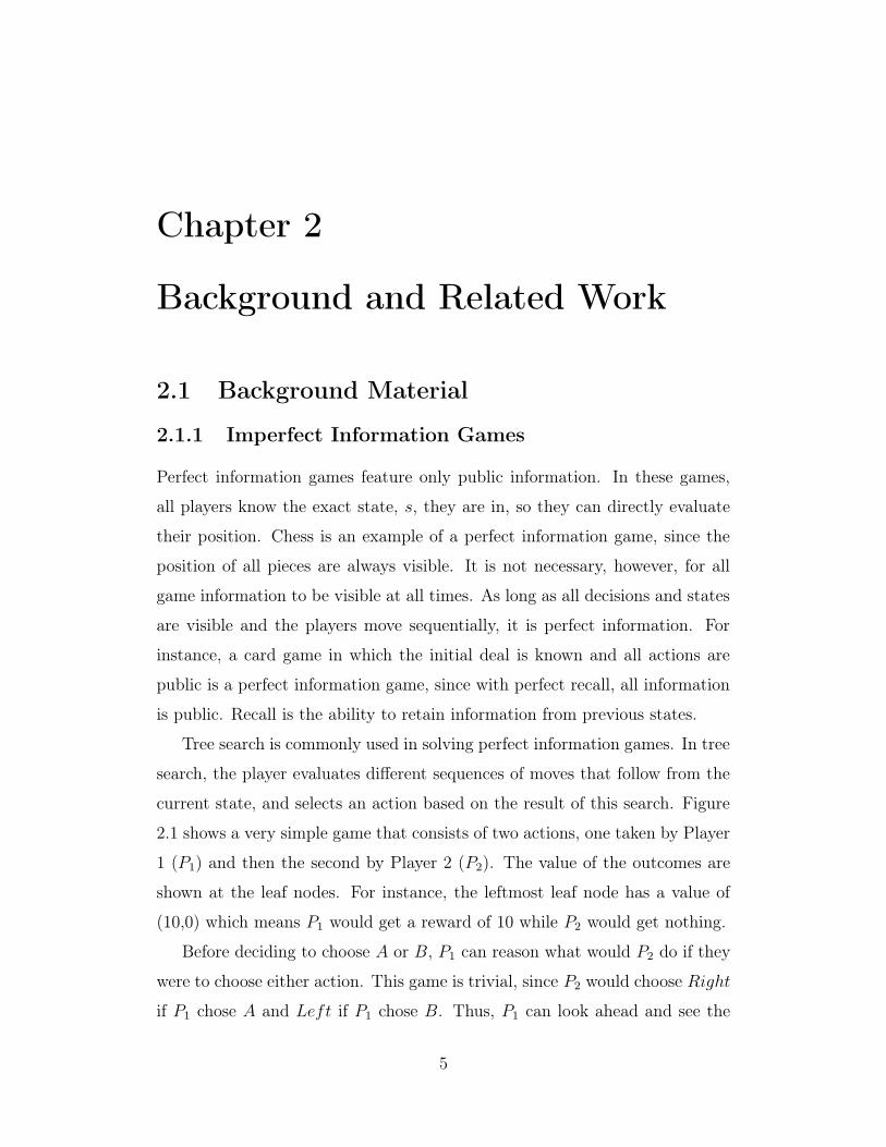
Tree search is commonly used in solving perfect information games. In tree
search, the player evaluates different sequences of moves that follow from the
current state, and selects an action based on the result of this search. Figure
2.1 shows a very simple game that consists of two actions, one taken by Player
1 (P1) and then the second by Player 2 (P2). The value of the outcomes are
shown at the leaf nodes. For instance, the leftmost leaf node has a value of
(10,0) which means P1 would get a reward of 10 while P2 would get nothing.
Before deciding to choose A or B, P1 can reason what would P2 do if they
were to choose either action. This game is trivial, since P2 would choose Right
if P1 chose A and Left if P1 chose B. Thus, P1 can look ahead and see the
5

P1
P2
(10, 0)
Left
(0, 1)
Right
A
P2
(1, 0)
Left
(0,−100)
Right
B
Figure 2.1: Simple Game tree for perfect information game.
only positive outcome happens if they choose B, resulting in a reward of 1.
This is a trivial example of lookahead search.
Imperfect information games feature private information. Due to this pri-
vate information, a player does not always know which state they are in, but
only which set of states they could be in which is termed the information set,
I. This causes problems with traditional search techniques, since the player
cannot directly perform search on the current state if they do not know what
the state is. Within this context, a player must infer the probability that they
are in a given state. When viewed from the start of the game, this is called
the reach probability, η.
Figure 2.2 shows an example of an imperfect information game tree. The
only difference in this game is that P2 does not observe the action of P1, so P2
does not know which of the two states they are in. These two states make up
an information set for P2 and it is demarcated with a dashed box in the tree.
Suppose you were P2, and you wanted to do a look ahead search. They only
problem is that you do not know what the next state will be, since you don’t
know where you are. While this problem can be solved using game theory, it
would suffice to say that it would be trivial to solve if P2 knew the probability
that they are in any given state. With this knowledge, they could simply find
the expected value of moving left or right and select the one with the greater
value.
6

P1
(10, 0)
Left
(0, 1)
Right
A
(1, 0)
Left
(0,−100)
Right
B
P2
Figure 2.2: An example of an imperfect information game. Tree is similar toFigure 2.1, but now P2 cannot distinguish between states inside the informationset (dotted rectangle) since they could not observe the private move made byP1.
2.1.2 Trick-taking Card Games
Card games are a prominent example of imperfect information games. Typi-
cally, players hold private information in the form of their hands, the hidden
cards they hold. Trick-taking card games like Contract Bridge, Skat, and
Hearts are card games in which players sequentially play cards to win tricks.
A trick leader plays a card, and the remaining players play a card in turn.
As the game progresses, information set sizes shrink rapidly due to hidden
information being revealed by player actions.
2.1.3 Skat
In this section I provide the reader with the necessary background related
to the three player trick-taking card game of Skat. Originating in Germany
in the 1800s, Skat is played competitively in clubs around the world. The
following is a shortened explanation that includes the necessary information
to understand the work presented here. For more in-depth explanation about
the rules of Skat, interested readers should refer to https://www.pagat.com/
schafk/skat.html.
Skat is played using a 32-card deck which is built from a standard 52-card
by removing 2,3,4,5,6 in each suit. A hand consists of each of the three players
being dealt 10 cards with the remaining two kept face down in the so-called
skat.
7

Games start with the bidding phase. In the cardplay phase, the winner of
the bidding phase plays as the soloist against the team formed by the other two
players. of the game. Upon winning the bidding, the soloist decides whether
or not to pickup the skat followed by discarding two cards face down, and
then declares what type of game will be played during cardplay. The game
type declaration determines both the rules of the cardplay phase and also the
score for each player depending on the outcome of the cardplay phase. Players
typically play a sequence of 36 of such hands and keep a tally of the score over
all hands to determine the overall winner.
The game value, which is the number of points the soloist can win, is the
product of a base value (determined by the game type, see Table 2.1) and
a multiplier. The multiplier is determined by the soloist having certain con-
figurations of Jacks and other high-valued trumps in their hand and possibly
many game type modifiers explained in Table 2.2. An additional multiplier is
applied to the game value for every modifier.
After dealing cards, the player to the right of the dealer starts bidding by
declaring a value that must be less than or equal to the value of the game he
intends to play — or simply passing. If the soloist declares a game whose value
ends up lower than the highest bid, the game is lost automatically. Next, the
player to the dealer’s left decides whether to accept the bid or pass. If the
player accepts the bid, the initial bidder must proceed by either passing or
bidding a higher value than before. This continues until one of the player’s
decides to pass. Finally, the dealer repeats this process by bidding to the player
who has not passed. Once two players have passed, the remaining player has
won the bidding phase and becomes the soloist. At this point, the soloist
decides whether or not to pick up the skat and replace up to two of the cards
in his hand and finally declares a game type.
Cardplay consists of 10 tricks in which the trick leader (either the player
who won the previous trick or the player to the left of the dealer in the first
trick) plays the first card. Play continues clockwise around the table until
each player has played. Passing is not permitted and players must play a card
of the same suit as the leader if they have one — otherwise any card can be
8

Table 2.1: Game Type Description
Base Soloist WinType Value Trumps Condition
Diamonds 9 Jacks and Diamonds ≥ 61 card pointsHearts 10 Jacks and Hearts ≥ 61 card pointsSpades 11 Jacks and Spades ≥ 61 card pointsClubs 12 Jacks and Clubs ≥ 61 card pointsGrand 24 Jacks ≥ 61 card pointsNull 23 No trump losing all tricks
Table 2.2: Game Type Modifiers
Modifier DescriptionSchneider ≥90 card points for soloistSchwarz soloist wins all tricks
Schneider Announced soloist loses if card points < 90Schwarz Announced soloist loses if opponents win a trick
Hand soloist does not pick up the skatOuvert soloist plays with hand exposed
played. The winner of the trick is the player who played the highest card in
the led suit or the highest trump card.
In suit and grand games, both parties collect tricks which contain point
cards (Jack:2, Queen:3,King:4,Ten:10,Ace:11) and non-point cards (7,8,9). Un-
less certain modifiers apply, the soloist must get 61 points or more out of the
possible 120 card points in the cardplay phase to win the game. In null games
the soloist wins if he loses all tricks.
Comparison to Contract Bridge
While Skat is a popular trick-taking card game, more research has been done
in Contract Bridge, a game with many similarities to Skat. For this reason,
I present a lot of related work in the domain of Contract Bridge. Both are
trick-based games featuring bidding and cardplay phases. The numerical Skat
bidding seems simpler than Bridge bidding because no bidding conventions
have to be followed and there is not much room (and incentive) in Skat to
convey hand information to other players. However, Skat adds uncertainty in
form of unknown Skat cards in the bidding phase. Other notable differences
include cardplay for points in Skat rather than achieving a certain number of
9

tricks, Skat’s hidden discard move, and changing coalitions versus fixed 2 vs. 2
team play in Contract Bridge.
2.2 Related Work
In this section, I will present prior work on trick-taking card games, use of su-
pervised learning from human data, inference in search, and finally the specifics
of the current state-of-the art computer Skat program.
One WBridge5 [WBr19] and Jack [Sof19] have had recent success in the
World Computer Bridge Championship [Fed19], but due to the commercial
natures of these AI systems, their implementation details are not readily avail-
able.
2.2.1 Determinized Search Techniques
Determinized search techniques seek to apply perfect information algorithms
to imperfect information games. In a perfect information game, a player always
know which state they are in, so they can perform a tree search rooted at the
current state. For an imperfect information game, the player only knows which
set of states they could possibly be in, the information set. As seen earlier,
this makes the naive application of the search impossible. Determinized search
techniques sidestep this issue by assuming a given s within I is the current
state (determinizing), and performing search rooted at this state. These search
techniques are split into two main parts, sampling and evaluation. Sampling is
the repeated determinization of the state, and evaluation is the determination
of the values of the possible actions through the use of search.
Long et al. [Lon+10] explain why trick-taking card games are an ap-
propriate setting for determinized search algorithms. These algorithms are
considered state-of-the-art in several trick-taking card games.
Perfect Information Monte Carlo Tree Search (PIMC)
PIMC [Lev89] is a form of determinized search in which all possible actions are
evaluated by sampling states from the current information state, and averaging
10

PIMC(InfoSet I, int n)for a ∈ A(I) do
v[a] = 0endfor i ∈ {1..n} do
s← Sample(I, p)for a ∈ A(I) do
v[a]← v[a] + PerfectInfoVal(s, a)end
endreturn argmaxav[a]
Algorithm 1: vanilla PIMC. In the algorithm, a is action, p is probability,and v is value.
the values over the states which were determined using perfect information
algorithms. Algorithm 1 is a basic version of PIMC.
The first successful application of determinized search in a trick-taking card
game was GIB [Gin01] in Contract Bridge with the of PIMC. PIMC has shown
great success in other trick-taking card games including Skat [Bur+09], and
Hearts [Stu08]. The current state-of-the-art for cardplay in Skat uses PIMC
[SRB19].
Monte Carlo Tree Search (MCTS)
MCTS [Cou06; KS06] has shown to be a very strong search algorithm for
perfect information games, as demonstrated by the strength of the AlphaGo
architecture in Go [Sil+16], Chess and Shogi [Sil+17]. Broadly speaking, it
works by maintaining search statistics for each node of the tree based upon
rollouts that passed through that node. UCT [KS06], a form of MCTS, chooses
actions in the rollouts by treating each decision as a bandit problem.
Determinized UCT applies UCT in the imperfect information domain by
determinizing the state for each rollout. Determinized UCT was applied to
Skat [SBH08] with little success. ISMCTS [CPW12] is the application of
MCTS to imperfect information games by maintaining nodes for information
sets as opposed to states as is normally seen in MCTS. ISMCTS still relies on
determinization of the state for each rollout. Singe Observer(SO)-ISMCTS is
11

the single observer variant, and works under the assumption that all moves are
fully observable. Multiple Observer(MO)-ISMCTS takes into account partially
observable moves, and maintains separate tree for each distinct observer.
Imperfect Information Monte Carlo Tree Search (IIMC)
Later, Imperfect Information Monte-Carlo Search [FB13] was introduced. This
replaces the perfect information evaluation, with an imperfect information
evaluation. For example, PIMC could be used for the the evaluation. This
was shown to be very effective in Skat [FB13], and is still the strongest card
player for Skat. The biggest issue with this method though is that its extremely
computationally expensive. Currently, it is not a feasible solution when time is
of importance, which is typically the case in an online decision making setting.
Issues with Determinized Search
In perfect information game trees, the values of nodes depend only on the
values of their children, but in imperfect information games, a node’s value
can depend on other parts of the tree. This issue, called non-locality, is one
of the main reasons why determinized search has been heavily criticized in
prior work [FB98; RN16]. The other main issue identified is strategy fusion.
The strategy for an information set should be the same for any state within
that set since they are indistinguishable by definition. However, during the
determinized rollouts the strategy is now specific to the state. Fusing these
strategies together does not necessarily provide a good overall strategy, and
clearly does not take into account the roll of hidden information.
2.2.2 Inference in Search
In the context of imperfect information games, inference is the reasoning that
leads to the beliefs held on other players’ private information. Inference helps
with non-locality by biasing state samples so that they are more probable with
respect to the actions that the opponent has made. This seems to improve the
overall performance of determinized algorithms. However, the gains provided
by inference come at the cost of increasing the player’s exploitability. If the
12

inference model is incorrect or has been deceived by a clever opponent, using
it can result in low-quality play against specific opponents.
Previous applications of determinized search in trick-taking card games
acknowledge the relationship between inference and playing performance. In
Skat, Kermit [Bur+09; FB13] used a table-based technique to bias state sam-
pling based on opponent bids and declarations. This approach only accounts
for a limited amount of the available state information and neglects important
inference opportunities that occur when opponents play specific cards. Solinas
et al. [SRB19] extend this process by using a neural network to make predic-
tions about individual card locations. By assuming independence between
these predictions, the probability of a given configuration was calculated by
multiplying the probabilities corresponding to card locations in the configura-
tion. This enables information from the cardplay phase to bias state sampling.
While this method is shown to be effective, the independence assumption does
not align with the fact that for a given configuration, the probability that a
given card is present is highly dependent on the presence of other cards. For
instance, their approach cannot capture situations in which a player’s actions
indicate that their hand likely contains either the clubs Jack or the spades
Jack, but not both.
While not providing the likelihood of states, rule based policies can be
used to bias the sampling of states in determinized algorithms. Ginsberg
[Gin01] uses rule based bidding in GIB to sample states that are consistent with
the assumed bidding policy of the other players within the PIMC algorithm.
Likewise, Amit and Markovitch [AM06] use a rule based policy for bidding
in Bridge to limit the number of inconsistencies in sampled worlds in their
proposed determinized search algorithm.
In other domains, Richards and Amir [RA07] model the opponent’s policy
using a static evaluation technique and then perform inference on the oppo-
nent’s remaining tiles given their most recent move in Scrabble.
Sturtevant and Bowling [SB06] build a generalized model of the opponent
from a set of candidate player strategies. My use of aggregated human data
could be viewed as a general model that captures common action preferences
13

from a large, diverse player base.
2.2.3 Counter Factual Regret (CFR)
CFR techniques [Zin+08] work by minimizing counterfactual regret. The coun-
terfactual value, vσ(I) is the expected payoff for a player if they took actions
to reach I multiplied by the reach probability η, given the strategy profiles σ
of all players. vσ(I, a) is the same, except that the player takes a at I. The
instantaneous regret is the difference of these two values, basically how much
the player regrets making the decision to choose a. The counterfactual regret
is the sum over these regrets. Regret matching [HM00] is typically used for
minimizing regret. CFR is shown to able to find an ϵ-Nash equilibrium for two
player zero sum games [Zin+08].
These techniques have proven to be very successful in Poker [BS18; Mor+17].
For larger games, the general approach for using CFR methods is to first ab-
stract the game into a smaller version of itself, solve that, and then map those
strategies back to the original game. This was the case for the Poker appli-
cations. This is problematic for trick-taking card games, such as Skat. With
the vast amount of possible holdings and the highly interactive nature of these
hands, creating good abstractions is very difficult. For example, for a given
game type, Skat has 225,792,840 possible holdings from the point of view of the
soloist after picking up the skat, much larger than the 1326 possible holdings
that a player has in Poker. Recent advances in Regression CFR [Wau+15] may
provide a means of using functional representation within the CFR framework
for Skat, but it is not clear how this would be effectively applied to a game of
this size.
2.2.4 Supervised and Reinforcement Learning
With the recent success in machine learning, directly applying supervised and
reinforcement learning to games has shown great promise. Within the domain
of perfect information games, the foundation of AlphaGo [Sil+16] was built
upon policy and value networks trained on expert human data. One prominent
14

use of learning in the context of trick-taking card games is for bidding, with
great success demonstrated in Contract Bridge.
Yeh et al. [YHL18] directly use reinforcement learning algorithms to learn
a value network for bidding in Bridge, however, this was limited to the case
where the opposing team always passes. While this greatly simplifies the
problem, it ignores key elements of the game. Rong et al. [RQA19] train
a network to predict the individual card locations and use this as an input
into the policy network. Both the inference network and the policy network
were trained using expert human data, but like [Sil+16], both the networks
are refined using reinforcement learning. While showing positive results, both
these contributions are evaluated on the double dummy results, a heuristic for
actual cardplay strength. This is done to avoid using search based algorithms
that are too costly to produce game play.
In the cardplay setting, Baier et al. [Bai+18] leverage policies trained from
supervised human data to bias MCTS results in the trick-taking card game
Factory Spades. This is similar to our approach in that it uses human data
to train an opponent model, but different because their model is not used to
infer opponent hidden information.
In the domain of Hanabi, Foerster et al. present Bayesian Auto Decoder
(BAD) a method of inference for cooperative multi-agent reinforcement learn-
ing problems [Foe+18]. Hanabi is a cooperative card game that features private
information, although interestingly enough a player’s hand is only kept from
themselves. By maintaining a public belief and shared policies, players are
able to better infer their holdings and the beliefs of others. While this line of
research seems promising, it is not obvious how to apply it to the adversarial
setting in Skat and Bridge.
2.2.5 State-of-the-Art in Skat
Previous work on Skat AI has applied separate solutions for decision-making
in the pre-cardplay and cardplay phases. The cardplay phase has received the
most attention — probably due to its similarity to cardplay in other trick-
taking card games.15

The current state-of-the-art for the pre-cardplay phase [Bur+09] uses PIMC
and evaluates the leaf nodes after the discard phase using the GLEM frame-
work [Bur98]. The evaluation function is based on a generalized linear model
over table-based features indexed by abstracted state properties. These tables
are computed using human game play data. Evaluations take the player’s
hand, the game type, the skat, and the player’s choice of discard into account
to predict the player’s winning probability. The maximum over all player
choices of discard and game type is taken and then averaged over all possible
skats. Finally, the program bids if the such estimated winning probability is
higher than some constant threshold.
Despite its shortcomings, PIMC Search [Lev89] continues be the state-of-
the-art cardplay method for Skat, with the determinized states solved using
minimax search. Inference is done using the card location method described
earlier [SRB19] and is used to bias the sampling of the states in the search
algorithm, so that the likelihood of sampling the state is proportional to the
estimated probability the player is in that state. When time for decision
making is not a factor,the current strongest computer Skat player uses IIMC
with PIMC used for the evaluation [FB13], however, I do not examine this
implementation in my thesis since I find it to be too computationally expensive
for an online player.
Together, the described solutions make up Kermit, the current strongest
Skat AI that has shown to play at expert human level strength [Bur+09].
16

Chapter 3
Imitation Based Policies forPre-Cardplay in Skat
It was the goal of the work in this chapter to produce strong and fast policies
for Skat using supervised learning on data from Skat games played between
humans. First, I describe the training of imitation networks using the data,
and how I use those networks to create pre-cardplay policies for Skat. Then,
I present a simple policy that selects the maximum output from the imitation
network that corresponds to a legal action. Next, I study the issue of overly
conservative bidding that comes as a result of the simple aforementioned policy,
and how I can remedy the issue. Finally, I explore using a value network in
conjunction with the imitation network for creating the declaration/pickup
phases’ policies, in order to perform better than using either separately.
3.1 Pre-cardplay Method
The pre-cardplay phase has 5 decision points: max bid for the Bid/Answer
Phase, max bid for the Continue/Answer Phase, the decision whether to pickup
the skat or declare a hand game, the game declaration and the discard. The
bidding phases feature sequential bids between two players, but further bids
can only be made if the other player has not already passed. This allows
a player to effectively pre-determine what their max bid will be. This ap-
plies to both the Bid/Answer and Continue/Answer phases. However, in the
Continue/Answer phase remaining players must consider which bid caused a
17

player to pass in the first bidding phase. The Declaration and Discard phases
happen simultaneously and could be modelled as a single decision point, but
for simplicity’s sake I separate them.
For each decision point, a separate DNN was trained using human data
from a popular Skat server, DOSKV [DOS18]. The server is open to the public,
thus the spread of skill levels is quite large. For discard, separate networks
were trained for each game type except for Null and Null Ouvert. These were
combined because of their similarity and the low frequency of Ouvert games
in the dataset.
The features for each network are one-hot encoded. The features and the
number of bits for each are listed in Table 3.1. The Bid/Answer network uses
the Player Hand, and Player Position features. The Continue/Answer network
uses the same features as Bid/Answer, plus the Bid/Answer Pass Bid, which
is the pass bid from the Bid/Answer phase. The Hand/Pickup network uses
the same features as Continue/Answer, plus the Winning Bid. The Declare
network uses the Player Hand + Skat feature in place of the Player Hand
feature, as the skat is part of their hand at this point. The Discard networks
use the same features as the Declare network, with the addition of the Ouvert
feature, which indicates whether the game is played with the soloist’s hand
revealed.
Note that the game type is not included in the feature set of the Discard
networks because they are split into different networks based on that context.
Assuming no skip bids (not normally seen in Skat) these features represent the
raw information needed to reconstruct the game state as observed from the
player. Thus, abstraction and feature engineering in this approach is limited.
The outputs for each network correspond to any of the possible actions
in the game at that phase. The legality of the actions depend on the state.
Table 3.2 lists the actions that correspond to the outputs of each network,
accompanied by the number of possible actions.
The networks all have identical structure, except for the input and output
layers. Each network has 5 fully connected hidden layers and use rectified linear
units (ReLU) [NH10]. The network structure can be seen in Figure 3.1. The
18

Table 3.1: Network input features
Features WidthPlayer Hand 32
Player Position 3Bid/Answer Pass Bid 67
Winning Bid 67Player Hand + Skat 32
Ouvert 1
Table 3.2: Corresponding actions to Network Outputs
Phase Action WidthBid/Answer MaxBid 67
Continue/Answer MaxBid 67Hand/Pickup Game Type or Pickup 13
Declare Game Type 7Discard Pair of Cards 496
Table 3.3: Pre-cardplay training set sizes and imitation accuraciesTrain Size Train Test
Phase (millions) Acc.% Acc.%Bid/Answer 23.2 83.5 83.2
Continue/Answer 23.2 79.7 80.1Pickup/Hand 23.2 97.3 97.3
Declare 21.8 85.6 85.1Discard Diamonds 2.47 76.3 75.7Discard Hearts 3.13 76.5 75.0Discard Spades 3.89 76.5 75.5Discard Clubs 5.07 76.6 75.8Discard Grand 6.21 72.1 70.3Discard Null 1.46 84.5 83.2
largest of the pre-cardplay networks consists of just over 2.3 million weights.
Tensorflow [Aba+16] was used for the entire training pipeline. Networks are
trained using the ADAM optimizer [KB14] to optimize cross-entropy loss with
a constant learning rate set to 10−4. The middle 3 hidden layers incorporate
Dropout [Sri+14], with keep probabilities set to 0.6. Dropout is only used for
learning on the training set. Each network was trained with early stopping
[Pre98] for at most 20 epochs. The size of the training sets, and accuracies
after the final epoch are listed for each network in Table 3.3. These accuracies
appear to be reasonable, given the number of options available at each decision
point. The test dataset sizes were set to 10,000. Training was done using a
19

OUTPUT
dropout
dropout dropout
FC-R
ELU
102
4
FC-R
ELU
102
4
FC-R
ELU
256
FC-R
ELU
512
FC-R
ELU
512
k-SO
FTM
AX
STAT
E FE
ATU
RES
Figure 3.1: Network architecture used across all game types for both soloistand defenders.
single GPU (Nvidia GTX 1080 Ti) and took around 8 hours for the training
of all pre-cardplay finalized networks.
These networks are optimized to predict what action a player from this
dataset would choose given a representation of the game context as an input,
which is done with the goal of using the networks to produce a policy that
is representative of the human players. For this reason, I refer to them as
imitation networks. One issue is that while the exact actions during the bid-
ding phase are captured, the intent of how high the player would have bid is
not. The intent is based largely on the strength of the hand, but how high
the player bids is dependent on the what point the other player passed. For
example, if a player decided their maximum bid was 48 but both other players
passed at 18, the maximum bid reached is 18. For this reason, the max bid
data was limited to the two players who passed in the bidding phase. The max
bid for these players is known since they either passed at that bid (if they are
the player to bid) or at the next bid (if they are the player to answer).
In the approach I chose, the output of the bidding networks corresponds to
the maxbid a player reached. The data is only representative of players who
20

passed in the bidding phase, and does not use the data of the bidding winner
since the maxbid they intended to reach is not available to train on. The
argmax on the outputs provides the most likely maxbid as predicted by the
network, but it would not utilize the sequential structure of the bids. What I
propose is to take the bid that corresponds to a given percentile, termed A. In
this way, the distribution of players aggressiveness in the human population
can be utilized directly to alter the aggressiveness of the player. Let B be the
ordered set of possible bids, with bi being the ith bid, with b0 corresponding
to passing without bidding. The maxbid is determined using
maxbid(s, A) = min(bi) s.t. Σij=0p(bj; θ|I) ≥ A (3.1)
where p(bj) is the output of the trained network, which is interpreted as the
probability of selecting bj as the maxbid for the given Information Set I and
parameters θ in the trained network. Given the returned maxbid bi and the
current highest bid in the game bcurr, the policy for the bidding player is
πbid(bi, bcurr) =
{bcurrent+1 if bi > bcurrentpass otherwise (3.2)
while the policy for the answer player is
πans(bi, bcurr) =
{yes if bi ≥ bcurrentpass otherwise (3.3)
Another limiting factor in the strength of direct imitation is that the policy
is trained to best copy humans, regardless of the strength of the move. While
the rational player would always play on expectation, it appears there is a
tendency for risk aversion in the human data set. For example, the average
human seems to play far fewer Grands than Kermit. Since Grands are high
risk / high reward, they are a good indication of how aggressive a player is.
To improve the pre-cardplay policy in the Hand/Pickup and Declare phases,
one can instead select actions based on learned values for each possible game
type. Formally, this policy is
πMV (I, a; θ) = argmax(v(I, a; θ)) (3.4)
21

where v is the output of the trained network for the given Information Set I,
action a, and parameters θ, and is interpreted as the predicted value of the
game.
Two additional networks were trained, one for the Hand/Pickup phase and
one for the Declare phase. These networks were identical to the previous
ones, except linear activation units are used for the outputs. The network
was trained to approximate the value of the actions. The value labels are
simply the endgame value of the game to the soloist, using the TP system.
For winning, the value is simply the TP awarded, but for losing the value is
the TP lost plus an additional negative 40 points in order to take into account
the defenders’ bonus for winning.
The loss was the mean squared error of prediction on the actual action
taken. For the Hand/Pickup network, the train and test loss were 607 and
623 respectively. For the Declare network, the values were 855 and 898. These
values seem quite large, but with the high variance and large scores in Skat,
they are in the reasonable range. For instance, the lowest base value for a
game is 18. If a player were to win this game, they would be awarded 68 TP.
If they were to lose, they would lose 108 TP and both their opponents would
gain 40 TP. Altogether, the smallest point swing in terms of relative standings
from a win to a loss is 208 points, which creates a potential for high values for
the squared error loss.
The πMV seen in Equation 3.4 is problematic. The reason for this is that
many of the actions, while legal, are never seen in the training data within a
given context. This leads to action values that are meaningless, which can be
higher than the other meaningful values. For example, Null Ouvert is rarely
played, has high game value and is most often won. Thus the network will
predict a high value for the Null Ouvert action in unfamiliar situations which
in turn are not appropriate situations to play Null Ouvert. This results in an
overly optimistic player in the face of uncertainty, which can be catastrophic.
This is demonstrated in the results section.
To remedy this issue, I decided to use the supervised policy network in
tandem with the value network. The probability of an action from the policy
22

network is indicative of how often the move is expected to be played given the
observation. The higher this probability is, the more likely the network has
seen a sufficient number of “relevant” situations in which the action was taken.
With a large enough dataset, I assume that probabilities above a threshold in-
dicate that there is enough representative data to be confident in the predicted
action value. 0.1 was chosen as the threshold. There is no theoretical reason
for this exact threshold, other than it is low enough that it guarantees that
there will always be a value we are confident in. Furthermore, the probability
used is normalized after excluding all illegal actions.
The policy for the Hand/Pickup and Declare phases using the method
described above is
πMLV (I, a; θ) = argmax(vL(I, a; θ)) (3.5)
wherevL(I, a; θ) =
{v(I, a; θ) if plegal(a; θ|I) ≥ λ−∞ otherwise (3.6)
in which plegal is the probability normalized over all legal actions and λ is a
constant set to 0.1 in our case.
3.2 Bidding Experiments
Since Kermit is the current strongest Skat AI system [Bur+09] [SRB19], it is
used as the baseline for the rest of this paper. Since the network-based player
learned off of human data, it is assumed that defeating Kermit is indicative
of the overall strength of the method, and not based on exploiting it’s specific
policy.
Because Skat is a 3-player game, each match in the tournament is broken
into six games. In a match, all player configurations are considered, with the
exception of all three being the same bot, resulting in six games (see Table 3.4).
In each game, once the pre-cardplay phase is finished, the rest of the game
is played out using Kermit cardplay, an expert level player based on PIMC
search which samples 160 worlds — a typical setting. The results for each bot
is the resultant average over all the games played. Each tournament was ran
23

Table 3.4: Player configurations in a single match consisting of six hands(K=Kermit, NW=Network Player)
Game Number Seat1 Seat2 Seat31 K K NW2 K NW K3 K NW NW4 NW NW K5 NW K NW6 NW K K
for 5,000 matches. All tournaments featured the same identical deals in order
to decrease variance.
Different variations of the pre-cardplay policies were tested against the
Kermit baseline. Unless otherwise stated, the policies use the aggressiveness
transformation discussed in the previous section, with the A value following
the policies prefix. The variations are:
• Direct Imitation Max (DI.M): selects the action deemed most probable
from the imitation networks
• Direct Imitation Sample (DI.S): like DI.M, but samples instead of taking
the argmax
• Aggressive Bidding (AB): like DI.M, but uses the aggressiveness trans-
formation in bidding
• Maximum Value (MV): like AB, but selects the maximum value action
in the Hand/Pickup and Declare phases
• Maximum Likely Value (MLV): like AB but uses the maximum likely
value policy, πMLV , in the Hand/Pickup and Declare phases
While the intuition behind the aggressiveness transformation is rooted in in-
creasing the aggressiveness of the bidder, the choice for A is not obvious. MLV
and AB were investigated with A values of 0.85, 0.89, 0.925. Through limited
trial and error, these values were chosen to approximately result in the player
being slightly less aggressive, similarly aggressive, and more aggressive than
24

Kermit’s bidding, as measured by share of soloist games played in the tourna-
ment setting. MV was only tested with A of 0.89 since it was clear that the
issue of overoptimism was catastrophic.
An overview of the game type selection breakdown is presented in Ta-
ble 3.5, while an overview on the performance is presented in Table 3.6. To
measure game playing performance I use the Fabian-Seeger tournament point
(TP) scoring system which awards the soloist (50 + game value) points if they
win. In the case of a loss, the soloist loses (50 + 2· game value) points and the
defenders are awarded 40 points. All tournament points per game (TP/G)
difference values reported were found to be significant, unless otherwise stated.
These tests were done using Wilcon signed-rank test [WKW70], with a signif-
icance level set to p=0.01. This test is valid for paired data that is on a ratio
scale and it does not assume a normal distribution. The data is paired since
the deal is the same for all games within a match and a ratio scale is used for
the scoring, thus the test is appropriate.
Clearly, naively selecting the max value (MV) in the Hand/Pickup and
Declare phases causes the bot to perform very poorly as demonstrated by it
performing -75.6 TP/G worse than the Kermit baseline. It plays 96% of its
suit games as hand games, which is extremely high to the point of absurdity.
In the previous section, I explained how actions that are not representative of
normal play in the dataset provide values that are overly optimistic, and these
results align with this explanation.
Direct Imitation Argmax (DI.M) performed much better, but still per-
formed slightly worse than the baseline by 2.1 TP/G. Direct Imitation Sample
(DI.S) performed 4.2 TP/G worse than baseline and slightly worse than DI.M.
The issue with being overly conservative is borne out for both these players
with the player being soloist approximately half as often as Kermit.
The direct imitation with the aggressiveness transformation (AB) per-
formed better than Kermit for the lower values, but slightly worse for AB.925.
None of these values were statistically significant. The best value for A was
0.85 (AB.85) which leads to +0.4 TP/G against Kermit. The advantage de-
creases with increasing A values. At the 0.85 A value, the player is soloist
25

a fewer of 1.81 times per 100 games played, indicating it is a less aggressive
bidder than Kermit.
The players selecting the max value declarations within a confidence thresh-
old (MLV) performed the best overall, outperforming the AB players at each
A value level. The best overall player against Kermit is the MLV.85 player. It
outperforms Kermit by 1.2 TP/G, 0.8 TP/G more than the best AB player.
The actual breakdown of games is quite interesting, as it shows that the
AB and MLV players are markedly different in their declarations. Across the
board, AB is more conservative as it plays more Suit games and less Grand
games (worth more and typically more risky) than the corresponding MLV
player.
These results indicate that the MLV method that utilizes the networks
trained on human data provides the new state-of-the-art for Skat bots in pre-
cardplay.
26

Table 3.5: Game type breakdown by percentage for each player, over their5,000 match tournament. Soloist games are broken down into types. Defensegames (Def) and games that were skipped due to all players passing (Pass) arealso included. The K vs X entries list breakdowns of Kermit playing againstplayer(s) X with identical bidding behavior.
Match Grand Suit Null NO Def PassDI.S 6.8 17.1 1.2 0.8 68.9 5.2DI.M 6.6 16.0 0.9 0.9 69.3 6.3MV.89 8.2 25.4 0.0 0.3 64.8 1.4MLV.85 10.6 19.0 1.6 1.3 65.6 1.9MLV.89 11.0 19.8 1.7 1.4 64.8 1.4MLV.925 11.6 20.5 1.8 1.5 63.6 1.1AB.85 8.7 21.5 1.1 1.2 65.6 1.9AB.89 9.2 22.3 1.1 1.2 64.8 1.4AB.925 9.7 23.1 1.2 1.3 63.6 1.1K vs DI.S 10.7 21.0 3.8 2.0 57.1 5.5K vs DI.M 10.7 21.6 3.8 2.0 55.5 6.4K vs *.85 11.0 17.5 2.5 1.8 64.9 2.4K vs *.89 10.9 16.8 2.2 1.8 66.4 1.9K vs *.925 11.0 15.8 2.0 1.7 68.0 1.5
Table 3.6: Tournament results over 5,000 matches between learned pre-cardplay polices and the baseline player (Kermit). All players use Kermit’scardplay. Rows are sorted by score difference (TP/G=tournament points pergame, S=soloist percentage) Starred TP/G diff. values were not found to besignificant at p=0.01.
Player (P) TP/G(P) TP/G(K) diff. S(P) S(K) diff.MV.89 -41.3 34.3 -75.6 33.8 31.7 2.1DI.S 19.2 23.3 -4.1 25.9 37.2 -11.3DI.M 20.6 22.7 -2.1 24.3 38.1 -13.8AB.925 22.4 22.6 -0.2∗ 35.3 30.5 4.9AB.89 22.9 22.5 0.4∗ 33.8 31.7 2.1AB.85 23.0 22.6 0.4∗ 32.5 32.8 -0.3MLV.925 23.0 22.3 0.8∗ 35.3 30.5 4.9MLV.89 23.3 22.3 1.0∗ 33.8 31.7 2.1MLV.85 23.6 22.4 1.2 32.5 32.8 -0.3
27

Chapter 4
Learning Policies from HumanData For Cardplay in Skat
4.1 Cardplay Method
With improved pre-cardplay policies, the next step was to create a strong
and fast cardplay policy using the human data. To do this, a collection of
networks were trained to predict the human play in the dataset using the
same network architecture used for the pre-cardplay imitation networks. Six
networks were trained in all; defender and soloist versions of Grand, Suit, and
Null. The networks take the game context encoded into features as the input,
and predicts the action the player would take as the output.
To capture the intricacies of the cardplay phase, handcrafted features were
used — they are listed in Table 4.1. Player Hand represents all the cards in the
players hand. Hand Value is the sum of the point values of all cards in a hand
(scaled to the maximum possible value). Lead cards represents all the cards the
player led (first card in the trick). Sloughed cards indicate all the non-Trump
cards that the player played that did not follow the suit. Void suits indicate the
suits which a player cannot have based on past moves. Trick Value provides
the point value of all cards in the trick (scaled to the max possible value).
Max Bid Type indicates the suit bid multipliers that match the maximum
bid of the opponents. For example, a maximum bid of 36 matches with both
the Diamond multiplier, 9, and the Clubs multiplier, 12. The special soloist
declarations are encoded in Hand Game, Ouvert Game, Schneider Announced,
28

Table 4.1: Network input features
Common Features WidthPlayer Hand 32Hand Value 1
Played Cards (Player, Opponent 1&2) 32*3Lead Cards (Opponent 1&2) 32*2
Sloughed Cards (Opponent 1&2) 32*2Void Suits (Opponent 1&2) 5*2
Current Trick 32Trick Value 1
Max Bid Type (Opponent 1&2) 6*2Soloist Points 1
Defender Points 1Hand Game 1Ouvert Game 1
Schneider Announced 1Schwarz Announced 1
Soloist Only Features WidthSkat 32
Needs Schneider 1
Defender Only Features WidthWinning Current Trick 1
Declarer Position 2Declarer Ouvert 32
Suit/Grand Features WidthTrump Remaining 32
Suit Only Features WidthSuit Declaration 4
and Schwartz announced. Skat encodes the cards placed in the skat by the
soloist, and Needs Schneider indicates whether the extra multiplier is needed
to win the game. Both of these are specific to the soloist networks. Specific to
the defenders are the Winning Current Trick and the Declarer Ouvert features.
Winning Current Trick encodes whether the current highest card in the trick
was played by the defense partner. Declarer Ouvert represents the soloist’s
hand if the soloist declared Ouvert. Trump remaining encodes all the trump
cards that the soloist does not possess and have not been played, and is used in
the Suit and Grand networks. Suit Declaration indicates which suit is trump
29

Table 4.2: Cardplay train/test set sizes
Train Size Train TestPhase (millions) Acc.% Acc.%
Grand Soloist 53.7 80.3 79.7Grand Defender 105.4 83.4 83.1
Suit Soloist 145.8 77.5 77.2Suit Defender 289.1 82.3 82.2Null Soloist 5.4 87.3 86.3
Null Defender 10.7 72.9 71.6
based on the soloist’s declaration, and is only used in the Suit networks. These
features are one-hot encoded, except for Trick Value, Hand Value, Soloist and
Defender points, which are floats scaled between 0 and 1. The network has 32
outputs — each corresponding to a given card.
The resultant data set sizes, and accuracies after the final epoch are listed
in Table 4.2. The test set had a size of 100,000 for all networks. The accuracies
are quite high, however, this doesn’t mean much in isolation as actions can be
forced, and the number of reasonable actions is often low in the later tricks.
Training was done using a single GPU (Nvidia GTX 1080 Ti) and took around
16 hours for the training of the finalized cardplay networks. The largest of the
cardplay networks consists of just under 2.4 million weights.
4.2 Cardplay Experiments
Bidding policies from the previous chapter, as well as original Kermit bidding,
were used in conjunction with the learned cardplay networks. The cardplay
policy (C) takes the argmax over the legal moves of the game specific network’s
output, and plays the corresponding card. AB and MLV bidding policies were
tested at all three bidding aggressiveness levels. I also tried sampling of the
policy network (CS), to see how it affected the play. The sampling was only
done for Kermit bidding as it performed worse than the argmax policy.
Each variant played against Kermit in the same tournament setup from
the previous section. Again, all TP/G difference reported were found to be
significant. Results are reported in Table 4.3. Again, the Wilcoxon signed-
30

Table 4.3: Cardplay tournament results over 5,000 matches between botsusing pre-cardplay policies from the previous section and the learned card-play policies. All variants were played against the baseline, Kermit(TP/G=tournament points per game, S=soloist percentage). All differencevalues ∆ were found to be statistically significant.
Player (P) TP/G(P) TP/G(K) ∆ S(P) S(K) ∆
K+C 21.9 24.6 -2.6 31.9 31.9 0.0K+CS 21.1 26.0 -4.9 31.9 31.9 0.0AB.89+C 22.4 24.5 -2.1 33.8 31.7 2.1AB.925+C 22.3 24.2 -1.9 35.3 30.5 4.9AB.85+C 22.6 24.4 -1.8 32.5 32.8 -0.3MLV.925+C 22.8 24.1 -1.3 35.3 30.5 4.9MLV.89+C 23.1 24.4 -1.3 33.8 31.7 2.1MLV.85+C 23.4 22.4 1.0 32.5 32.8 -0.3
rank test is used for all TP/G difference values reported with a significance
level of 0.01.
The strongest full network player was MLV.85+C, and it outperformed
Kermit by 1.0 TP/G. All the rest of the cardplay network players performed
worse than Kermit. Like the bidding results, all MLV players performed bet-
ter than all AB players. Kermit’s search based cardplay is quite strong, and
it appears to be stronger than the imitation cardplay, as demonstrated by it
outperforming K+C by 2.6 TP/G. The sampling variant K+CS performed 4.9
TP/G worse than the search based method. I propose two main explanations
for why argmax performs better than sampling; keeping the trajectory within
a space closer to the training set and avoiding mistakes. The trajectory ex-
planation comes from the idea that by choosing a more likely action given
a world, we have a greater chance of transitioning to a state that resembles
worlds that we have seen. The mistake avoidance argument rests on the idea
that if human players randomly make mistakes, these mistakes would appear
as a noisy training signal. By taking the most likely action, we are effectively
filtering out this noise. The overall poorer performance of the cardplay pol-
icy is probably due to the effectiveness of search to play near perfectly in the
later half of the game when a lot is known about the hands of the players.
While these results are compelling, it should be noted that further investiga-
31

tion into the interplay between the bidding and cardplay policies is required
to get a better understanding of their strengths. One advantage the imitation
network cardplay has is that its much faster, taking turns at a constant rate
of around 2.5 ms, as compared to Kermit which takes multiple seconds on the
first trick, and an average time of around 650 ms (both using a single thread
on consumer-level CPU).
To investigate the assumption that the search based method is stronger
in the later stages of the game, I performed experiments using hybridized
players. These players used the learned cardplay policy up to a given trick,
and the Kermit cardplay after that. Unlike the previous experiments, I used
the mirrored adversarial tournament setup. Two games are played per match;
player A plays as soloist against two clones of player B and the reverse of that.
All matches start at cardplay, and feature the same starting positions that
have been created using Kermit pre-cardplay policies. 9 tournaments were
ran, with the Kermit policy taking over after varying trick numbers. This
ranged from the starting at the first trick, to not starting at all. The results
are shown in Table 4.4. Hybrid-1 performs the strongest, with a +0.7 TP/G
over Kermit. It is not significant at p = 0.01, however the p value is still quite
small at 0.028. As the cardplay policy is used further along into the game
past the first trick, the performance decreases. This fits with the theory that
search based methods are stronger in later stages of the game.
Since I used the mirrored setup, I could separate the defense and soloist
play. In this way, I could see how the combination of different hybridizations
for soloist and defense would perform. The difference in TP/G for each combi-
nation is shown in Table 4.5, with positive values indicating that the hybridized
combination outperforms Kermit. Def0-Sol0 is actually pure Kermit since Ker-
mit takes over prior to the first trick for both soloist and defense. The reason
why it performs worse than it’s identical counterpart can be attributed to the
randomness in the sampling of worlds. The strongest cardplayer combination
is Def1-Sol3 which outperforms Kermit by 0.9 TP/G.
32

Table 4.4: Cardplay tournament results over 5,000 matches between botsusing pre-cardplay policies from the previous section and the learned card-play policies. All variants were played against the baseline, Kermit(TP/G=tournament points per game, S=soloist percentage). Difference values∆ not found to be statistically significant at p=0.01 have been starred.
Player (P) TP/G (P) TP/G (K) ∆ TP/GHybrid-0 22.1 22.1 -0.1∗
Hybrid-1 22.3 21.5 0.7∗
Hybrid-2 22.1 21.7 0.3∗
Hybrid-3 22.2 21.9 0.3∗
Hybrid-4 21.8 22.4 -0.5∗
Hybrid-5 21.5 23.0 -1.5Hybrid-6 20.6 23.8 -3.1Hybrid-7 20.0 24.8 -4.7Hybrid-8 20.0 25.1 -5.2Hybrid-9 19.8 25.3 -5.5
Table 4.5: Mirrored cardplay tournament results over 5,000 matches betweenKermit and hybridized bots. DefX indicates that the hybridized bot used theKermit card player starting at trick X for defense and the learned policy prior.SolX indicates the same thing, except in the soloist context. All values arehow many TP/G the hybridized bot outperformed Kermit. All pre-cardplaydone using Kermit.
Def0 Def1 Def2 Def3 Def4 Def5 Def6 Def7 Def8 Def9Sol0 -0.1 0.7 0.5 0.2 -0.4 -1.2 -2.1 -3.3 -3.7 -4.0Sol1 -0.1 0.7 0.5 0.2 -0.4 -1.2 -2.1 -3.3 -3.7 -4.0Sol2 -0.3 0.5 0.3 -0.1 -0.6 -1.4 -2.3 -3.5 -3.9 -4.2Sol3 0.1 0.9 0.6 0.3 -0.3 -1.1 -1.9 -3.2 -3.6 -3.9Sol4 -0.2 0.6 0.4 0.0 -0.5 -1.3 -2.2 -3.4 -3.8 -4.1Sol5 -0.4 0.4 0.2 -0.2 -0.8 -1.5 -2.4 -3.6 -4.0 -4.3Sol6 -1.1 -0.3 -0.5 -0.9 -1.5 -2.3 -3.1 -4.4 -4.8 -5.1Sol7 -1.5 -0.7 -0.9 -1.3 -1.9 -2.7 -3.5 -4.7 -5.2 -5.4Sol8 -1.5 -0.7 -0.9 -1.3 -1.9 -2.6 -3.5 -4.7 -5.2 -5.4Sol9 -1.6 -0.8 -1.0 -1.4 -2.0 -2.8 -3.6 -4.8 -5.3 -5.5
33

Chapter 5
Policy Based Inference in Skat
In the previous two chapters I have demonstrated that neural networks trained
off of human data can be used to create strong policies for the game of Skat.
While these policies can be used directly, the search based method proves to
be stronger in the cardplay portion of Skat. It is the goal of the work in
the chapter to improve the strength of the inference used in the search based
method. In this section, I present an algorithm that uses these policies to
improve inference in these games. As explained earlier, inference is a key part
of determinized search and specifically, in the search based cardplay in Kermit.
5.1 Inference Method
To determine the probability of a given state s in an information set I, we
need to calculate its reach probability η. If we can perfectly determine the
probability of each action that leads to this state, we can simply multiply all
the probabilities together and get η. Each s in I has a unique history h, the
sequence of all previous s and a that lead to it. h · a represents the history
appended with the action action taken at that state. Thus, there is a subset
of h, containing all the h · a for a given s. Formally:
η(s|I) =∏h·a⊑s
π(h, a) (5.1)
For trick-taking card games, the actions are either taken by the world
(chance nodes in dealing), other players’ actions, and our actions. Transition
34

EstimateDist(InfoSet I, int k, OppModel π)S ← SampleSubset(I, k)for s ∈ S do
η(s)← 1for h, a ∈ StateActionHistory(s) do
η(s)← η(s) ∗ π(h, a)end
endreturn Normalize(η)
Algorithm 2: Estimate the state distribution of an information set givenan opponent model and the actions taken so far.
probabilities of chance nodes can be directly computed since these are only
related to dealing, and the probability of our actions can be taken as 1 since we
chose actions that lead to the given state with full knowledge of our own policy.
This leaves us with determining the move probability of the other players. If we
have access to the other players’ policies, we can use Equation (5.1) to perfectly
determine the probability we are in a given state within the information set. If
we repeat this process for all states within the information set, we can calculate
the probability distribution across states. If we can perfectly evaluate the
value of all the state-action pairs, we can select the action that maximizes this
expected value which provides an optimal solution.
There are two main issues with this approach. The first is that we either
do not have access to the other players’ policies, or they are expensive to
compute. This makes opponent/partner modelling necessary, in which we
assume a computationally inexpensive model of the other players, and use
them to estimate the reach probability of the state. The second problem is
that the number of states in the information set can be quite large. To get
around this, one can sample the worlds and normalize the distribution over the
subset of states. Because in Skat the information set size for a player prior to
card-play can consist of up to 281 billion states, we employed sampling. I use
Algorithm 2 to estimate a state’s relative reach probability. When sampling
is not needed, this becomes an estimate of the states true reach probability.
While I have access to the policy of the current strongest Skat bot, using
35

its policy directly would be computationally intractable because it uses an
expensive search based method that also performs inference. Also, it is the
goal of this research to develop robust inference that is not based upon the
play of a single player. Thus, I decided to use policies learned directly from
a large pool of human players. These policies are parameterized by the deep
neural networks trained on human games seen in the previous chapters. The
features for the pre-cardplay networks are a lossless one-hot encoding of the
game state while considerable feature engineering was necessitated for the
cardplay networks. Separate networks were trained for each distinct decision
point in the pre-cardplay section, and for each game type for the cardplay
networks. More details on the training and the dataset can be found in the
previous chapters.
The decision points in pre-cardplay are bidding, picking up or declaring a
hand game, choosing the discard, and declaring the game. The decision points
in the cardplay section are every time a player chooses what card to play. While
inference would be useful for decision-making in the pre-cardplay section, we
are only applying it to cardplay in this paper. As such, one can abstract
the bidding decisions into the maximum bids of the bidder and answerer in
the bid/answer phase, and the maximum bids of bidder and answerer in the
continue/answer phase. For these maximum bid decision points, the maximum
bid is only observable if the player passes. For the cases in which the intent of
maximum bid is hidden, the probability attached to that decision point is the
sum of all actions that would have resulted in the same observation, namely
the probability of all maximum bids greater than the pass bid. The remaining
player decision points are pickup or declare a hand game, discard and declare,
and which card to play. As these are not abstracted actions, the probability
of the move given the state can be determined directly from the appropriate
imitation network detailed in the previous section.
The current state-of-the-art Skat bot, Kermit, uses search-based evaluation
that samples card configurations. A card configuration is the exact location
of all cards, and thus doesn’t take into account which cards where originally
present in the soloist’s hand prior to picking up the skat. Depending on the
36

game context, there are either 1 or 66 (12 choose 2) states that correspond to
a card configuration during the cardplay phase. Two variants of inference were
explored. The first variant samples card configurations. Decision points are
ignored for inference if there are multiple states with the same card configura-
tion but different features (input to the network). The second variant samples
states directly, thus avoiding this issue. For this implementation, the need to
distinguish states that share a configuration only occurs when a player does
inference on the soloists actions prior to picking up the two hidden cards in
the skat. Sampling card configurations will be treated as the default approach
for PI. When states are sampled instead, the inference will be labelled PIF,
for Policy Inference Full.
5.2 Direct Inference Evaluation
In this section, I test the quality of the inference directly. These inference mod-
ules are the original Kermit Inference (KI) [Bur+09], card-location inference
(CLI) [SRB19], and no inference (NI).
To measure the inference quality directly, I measured the True State Sam-
pling Ratio (TSSR) [SRB19] for each main game type, separately for defender
and soloist. TSSR measures how many times more likely the true state will
be selected than uniform random.
TSSR = η(s∗|I) / (1/|I|) = η(s∗|I) · |I| (5.2)
η(s∗|I) is the probability that the true state is selected given the information
set I, and |I| is the number of possible states. Since the state evaluator of
Kermit does not distinguish between states within the same card configuration,
I will slightly change the definition to measure how many times more likely
the card configuration (world) will be sampled than uniform random.
Since the players tested use a sampling procedure when the number of
worlds is too large, the TSSR value cannot easily be directly computed as
this would require all the world probabilities to be determined. I therefore
estimate it empirically. Since sampling was performed without replacement,
37

I use the given inference method to evaluate η given that the true world was
sampled k times. The resulting values can combined to get the combined
probability that the true world is selected:
TSSR = |I| · ΣkBinDist(k, p) · k · η(s∗|I, k) (5.3)
where BinDist is the probability mass of the binomial distribution with k
successes and probability of sampling the true world p which is 1/|I|. Terms of
the summation were only evaluated if the BinDist(k, p) value were significant,
which I cautiously thresholded at 10−7.
When the number of worlds is less than the set threshold parameter specific
to the player, all the worlds are sampled directly to compute the value. For
the sake of the TSSR experiments, null games were further subdivided into
the two main variants, null and null ouvert. Null ouvert is played with an
open hand for the soloist, thus making the inference quite different from that
of regular null games from the perspective of the defenders. For each game in
the respective test set, the TSSR value was calculated for each move for the
soloist, and one of the defenders. The test set was taken from the human data,
and was not used in training. The number of games in the test sets were 4,000
for grand and suit, 3,800 for null, and 13,000 for null ouvert.
Figure 5.1 shows the average TSSR metric after varying number of cards
have been revealed. The inference variants tested are PI20, PIF20, PI100,
CLI, and KI. NI was not tested because it will always have a value of 1. PI20
and PI100 sample 20,000 and 100,000 card configurations respectively, while
PIF20 samples 20,000 states. CLI samples 500,000 card configurations, and KI
samples 3200 card configurations in soloist, and a varying number in defense.
CLI inference was not implemented for null ouvert.
TSSR is higher on defense, with the exception of null ouvert. This is likely
due to there being many more possible worlds in the defenders information
set because of the hidden cards in the skat. Also, the defender can use the
declaration of the soloist for inference, which is a powerful indicator of the
soloist’s hidden cards. Null ouvert does not follow this trend because there
are only 66 possible worlds at most in defense while there are 184,756 for the38

Soloist Defender
(a) Grand
(b) Suit
(c) Null
(d) Null Ouvert
Figure 5.1: Average TSSR after Card Number cards have been played. Datais separated by game type and whether the player to move is the soloist (left)or a defender (right). 39

soloist. This allows for higher TSSR values for the soloist.
PI20, PIF20, and PI100 all achieve significantly higher TSSR values than
the other methods, across all game-types and roles. KI performs better than
CLI at the beginning of games, but surpasses KI once more cards are played.
PI100 appears to consistently perform better in defense than the other
Policy Inference variants, while PIF20 appears to perform slightly better than
PI20 in the first half of defender games, but not significantly so. All TSSR
values trend down to 1 at the endgame, as the number of possible worlds
approaches 1.
One common feature across all games is the spiking of TSSR values, which
is best exemplified in suit games. The spiking is consistent between players
within the same game type and role graph. However, between graphs it is
not consistently occurring at the same number of cards played. I do not see
an obvious reason for this. However, these tests were done on human games
and thus I am not controlling for inherent biases in the distribution. Further
investigation is needed to determine why these spikes occur.
It is clear from these results that the Policy Inference approach provides
larger TSSR values, since the error envelopes are completely separated in the
figure. It also should be noted that perfect inference would not result in the
upper bound TSSR value which is equal to the number of worlds. Even with
perfect knowledge of the opponents’ policies, uncertainty is inherent and thus
a player with perfect TSSR value is not possible.
40

Chapter 6
Applying Policy Based Inferencein Determinized Search
With the vastly improved inference from the previous chapter, I investigate the
effect of applying the PI algorithm in the PIMC search that had already been
implemented in the Kermit AI system. It is the goal of this work to improve the
state-of-the art cardplay system by improving the inference in that system. As
explained earlier, the inference can be used to bias the sampling of the states
in the determinizing step of PIMC.
6.1 Cardplay Tournament
To test the performance of PI in cardplay, we played 5,000 matches for each
of suit, grand, and null games between the baseline players and the PI based
player in a pairwise setup. Only the cardplay phase of the game is played, while
the bidding and declaration is taken directly from the human data-set. These
games were held out from the policy training set. In a match, each player
will play as soloist against two copies of the opponent, as well as against two
copies of itself. The baseline players are all versions of Kermit, with the only
difference being the inference module used. These inference modules are KI,
CLI, with the addition of no inference (NI). This experiment is designed to see
if (a) the performance of the player improves as measured by its play against
opponents and (b) to determine the extent to which the defender and soloist
performance is responsible for this difference.
41

For each match-up I report the average tournament points per game (TP/G)
for the games in which the players played against each-other. The games in
which the player played against a copy of itself were used to determine the
difference in the effectiveness of the defenders and soloists.
AvBB denotes a match-up in which the soloist is of type A while the
defenders are both of type B. The value of the game AvBB is in terms of the
soloist score, therefore it is the sum of the soloist’s score and the negation of
the defenders’ score. In this notation, the performance of player A relative to
player B is given as
∆TP/G = [AvBB − BvAA]/3 (6.1)
The value is divided by 3 since it is enforced that a player is soloist 1/3
the time in the tournament setup. To directly compare the performance of
the defenders, one can measure the performance difference between scenarios
where the only difference is the change in defenders.
∆Def/G = [(AvBB +BvBB)− (AvAA+BvAA)]/6 (6.2)
A negative value for ∆Def/G indicates A performs better than B in defense.
The same concept can also be applied to directly compare the efficacy of the
soloist.
∆Sol/G = [(AvAA− BvAA) + (AvBB − BvBB)]/6 (6.3)
A positive value for ∆Sol/G indicates A performs better than B as the soloist.
The results for the tournament match-ups are shown in Table 6.1. All ∆
values reported have a ∗ attached if they are not found to be significant at a
p value of 0.01 when a Wilcoxon signed-rank [WKW70] test was performed.
This test is valid for paired data that is on a ratio scale and does not assume
a normal distribution. The data is paired since the pre-cardplay is the same
for all games within a match and a ratio scale is used for the scoring, thus the
test is appropriate.
The general trend is that PI performs the best, followed by CLI, then
KI, then NI. This fits with the expectation that better TSSR values seen in
42

Table 6.1: Tournament results for each game type. Shown are average tourna-ment scores per game for players NI (No Inference), CLI (Card-Location Infer-ence), PI (Policy Inference), and KI (Kermit’s Inference) which were obtainedby playing 5,000 matches against each other, each consisting of two games withsoloist/defender roles reversed. The component of ∆TP attributed to Def andSol is also indicated
Matchup Game Type TP ∆ TP ∆ Def ∆ Sol
KI : CLISuit 17.6 : 20.8 -3.2 -2.8 -0.4∗
Grand 37.0 : 39.0 -2.0 -1.8 -0.1∗
Null 17.2 : 19.8 -2.6 -2.7 0.1∗
KI : PISuit 16.5 : 21.6 -5.1 -4.2 -0.9
Grand 36.4 : 39.6 -3.1 -2.3 -0.8∗
Null 17.3 : 19.7 -2.4 -2.9 0.6∗
NI : CLISuit 16.1 : 24.1 -8.0 -7.4 -0.6∗
Grand 36.6 : 40.5 -3.9 -3.4 -0.5∗
Null 16.0 : 22.5 -6.5 -6.6 0.1∗
PI : CLISuit 19.5 : 17.2 2.3 1.6∗ 0.7∗
Grand 37.9 : 37.2 0.6∗ 0.2∗ 0.5∗
Null 18.8 : 17.3 1.6 1.1 0.4∗
KI : NISuit 23.3 : 18.6 4.6 4.5 0.1∗
Grand 39.7 : 38.4 1.3 1.3 0.1∗
Null 21.6 : 17.8 3.8 3.9 -0.0∗
NI : PISuit 14.6 : 25.0 -10.4 -9.1 -1.4
Grand 36.5 : 40.0 -3.6 -3.1 -0.4∗
Null 15.8 : 22.1 -6.3 -6.8 0.5
Figure 5.1 would translate into stronger game performance. Another inter-
esting result is that the majority of the performance gain seems to be from
the defenders, as demonstrated by the ∆Def values being consistently larger
than the ∆Sol values. The most interesting match-up is PI : CLI since it
roots the previous state-of-the-art skat inference against the new policy-based
method. PI outperforms CLI by 2.3, 0.6, and 1.6 TP/G in suit, grand, and
null, respectively. The grand result did not provide statistical significance.
The major drawback of the PI inference is the runtime. When combined
with evaluation, PI20 takes roughly 5 times longer to make a move than CLI.
43

Table 6.2: Tournament results for each game type. Shown are average tour-nament scores per game for players CLI (Card-Location Inference), PI20 (Pol-icy Inference with 20,000 card configurations sampled), PIF20 (Policy Infer-ence with 20,000 states sampled), PI20 (Policy Inference with 100,000 cardconfigurations sampled), and C (Cheating Inference) which were obtained byplaying 5,000 matches against each other, each consisting of two games withsoloist/defender roles reversed.
Game Type Suit Grand NullMatchup TP ∆ TP TP ∆ TP TP ∆ TP
PI : CLI 19.5 : 17.2 2.3 37.9 : 37.2 0.6∗ 18.8 : 17.3 1.6PIF20 : CLI 19.3 : 17.7 1.6 37.7 : 37.2 0.5∗ 18.0 : 17.7 0.3∗
PI100 : CLI 19.5 : 16.7 2.9 38.2 : 36.1 2.1 18.1 : 17.1 1.0∗
C : CLI 14.7 : 18.0 -3.3 30.0 : 38.5 -8.5 20.8 : 11.0 9.8PI : CLI (6way) 19.1 : 17.8 1.2 37.6 : 37.3 0.4∗ 18.3 : 17.7 0.6
Further experiments were conducted to test the effect of increasing the
number of sampled worlds to 100,000 (PI100) and sampling states instead
of card configurations (PIF20). In addition, a cheating version of Kermit was
introduced (C) in which it places all probability on the true state. All programs
were tested against CLI with only the mirrored adversarial setup used. The
rest of the experimental setup was identical.
The results in Table 6.2 indicate that PI100 performs stronger than the
other PI variants in suit and grand, when playing against CLI, however, only
the grand result is significantly better. The opposite is true for null, in which
PI20 performs strongest out of the PI variants. This result contradicts the
idea that a higher TSSR value necessarily corresponds to better cardplay per-
formance. Cheating inference performs worse than CLI in all but null games.
This is interesting because it puts all the probability mass on the true world,
but still plays worse than a player that is not cheating. This result in con-
junction with the worse null game score for PI100 indicates that further inves-
tigation into the exact role inference quality has within the context of PIMC
is required. Also, PI20 outperforms PIF20 over all game types, showing that
there can be benefits to sampling card configurations instead of states when
44

Table 6.3: Tournament results for each game type in the 6-way match betweenCLI and PI20. 5,000 matches were played for each game type.
Game Type ∆Sol ∆DefCLI ∆DefPI
Suit 1.0 -1.1 0.6*Grand 0.4* 0.0* 0.2*Null 0.2* -0.6* 0.5*
there is a limited sampling budget.
One further experiment was performed to determine whether performance
gains would be present with mixed defenders. This is interesting since it is pos-
sible the gain would only be present if the partner’s inference was compatible
with their own. For the sake of time, this was only done for the CLI and PI20
matchup. The added arrangements are AvAB, AvBA, BvAB, and BvBA.
With these added, we now have six games for each tournament match. The
results for this match-up are included in Table 6.2. PI is consistently stronger
than CLI (the grand result is not significant), but the effect size is smaller.
This is expected because PI is now defending against PI in the mixed setup
games. To further analyze the the relative effectiveness of the players as soloist
against only the mixed team defenders, we can calculate:
∆Sol = [(AvAB − BvAB) + (AvBA− BvBA)]/6 (6.4)
A positive value for ∆Sol means that PI is more effective than CLI as soloist in
the mixed setting. ∆DefB measures the difference in effectiveness of a mixed
defense (A and B) and a pure defense of A’s. It is calculated by averaging the
effect of swapping in player B into defense for all match-ups that included two
A’s on defense. The reverse can be done to find the effect of swapping in A to
form a mixed defense. A positive value for ∆DefPI means defense improved
when it was added, and same for ∆DefCLI .
While all the values in Table 6.3 show the same trends of PI performing
better on defense and soloist across all game types, the effect is only statisti-
cally significant for ∆Sol and ∆DefCLI in the suit games.
45

Chapter 7
Conclusion
In this thesis I have demonstrated that pre-cardplay policies for Skat can be
learned from human game data and that it performs better than Kermit’s
pre-cardplay — the prior state-of-the-art. Naively imitating all aspects of
the pre-cardplay by taking the argmax over the legal actions (DI-M) resulted
in a bidding policy that performed an average of 2.1 TP/G worse than the
Kermit baseline. The same procedure but with sampling (DI-S) resulted in the
player performing 4.1 TP/G worse than baseline. Using the novel method to
increase the aggressiveness of the bidder led to it performing 0.4 TP/G better
than the baseline, with A set to 0.85 (AB.85). Using this in conjunction with
game declaration based on the predicted values and probabilities of actions
(MLV.85), resulted in the best overall pre-cardplay policy, beating the baseline
by 1.2 TP/G. Also, the time for pre-cardplay decisions are much faster, as it
does not rely on search.
The direct imitation cardplay policy decreases the strength of the overall
player, performing 2.8 TP/G worse than the Kermit player when utilizing the
Kermit bidder. The best overall full network based player was MLV.925+C,
which outperformed Kermit by 1.0 TP/G. This full network player is order
of magnitudes faster than the search based player, and in this tournament
setup, performs better. One drawback is that while more computation can
be done to improve the search (improving the number of worlds sampled for
example), the same cannot be done for the network player. While the learned
cardplay policy was shown to be weaker overall than the search based method,
46

the hybrid player that uses the policy then switches over to search after a few
moves is shown to be stronger than the search based policy alone.
Policy Inference (PI) appears to provide much stronger inference than its
predecessors, namely Kermit Inference (KI) and Card Location Inference (CLI)
as demonstrated by the TSSR value figures. Across the board, the higher
TSSR values translate into stronger game-play as demonstrated in card-play
tournament settings. PI20 outperforms CLI by 2.3, 0.6, and 1.6 TP/G in
suit, grand, and null games, respectively. Also, it seems that increasing the
number of states sampled increases the performance of PI, however, this did
not translate into the null game type. Further investigation into this null
game result is needed. I would expect that when substantially increasing the
sampling threshold, the state sampling employed by PIF20 would be more ef-
fective. But under this limited sampling regimen, sampling card configurations
is more effective than sampling states.
7.1 Future Work
Now that success has been established for training model-free policies from
human data in Skat, the next logical step is to improve these policies di-
rectly through experience similar to the process shown in the original AlphaGo
[Sil+16]. In [Sri+18] regret minimization techniques often used to solve im-
perfect information games are related to model-free multi-agent reinforcement
learning. The resulting actor-critic style agent showed fast convergence to ap-
proximate Nash equilibria during self-play in small variants of Poker. Applying
the same approach may be difficult because of Skat’s size and the fact that it
is not zero-sum, but starting with learning a best response to the full imitation
player discussed in this work should be feasible and may yield a new state-of-
the-art player for all phases of the game. The next step would be to create a
fully-fledged self-play regime for Skat. Learning policies through self-play has
shown to yield strategies that are “qualitatively different to human play” in
other games [Sil+17]. This could be problematic because Skat involves coop-
eration on defense during the card play phase. Human players use conventions
47

and signals to coordinate and give themselves the best chance of defeating
the soloist. In order to play well with humans, policies need to account for
these signals from their partner and send their own. Continually incorporating
labelled data from human games may help alleviate this problem.
Also, with a strong and fast network based policy, the IIMC Skat player
[FB13] can be sped up by using the network player for the lower level imperfect
information algorithm. The policy can also be used for move ordering and
pruning in the existing search based methods.
Future work related to inference in trick-taking card games should focus on
the relationship between opponent modelling and exploitability. In particular,
measuring the exploitability of our current policy trained from human data
to see how our algorithm would fare against the worst-case opponent could
lead to insight regarding the robustness of our approach. Likewise, adjusting
player models online could enable us to better exploit our opponents and
cooperate with team-mates. Another direction is to experiment with heuristics
that allow our algorithm to prune states that are highly unlikely and stop
considering them altogether. This could help us sample more of the states
that are shown to be realistic given our set of human games and possibly
improve the performance of the search.
And finally, testing the current iteration of Kermit against human players
would be illuminating, as the strength has dramatically improved since the
last time it was measured against human experts [Bur+09].
48

References
[Aba+16] Martn Abadi, Paul Barham, Jianmin Chen, Zhifeng Chen, AndyDavis, Jeffrey Dean, Matthieu Devin, Sanjay Ghemawat, GeoffreyIrving, Michael Isard, et al. “Tensorflow: A System for Large-scaleMachine Learning.” In: OSDI. Vol. 16. 2016, pp. 265–283. 19
[AM06] Asaf Amit and Shaul Markovitch. “Learning to Bid in Bridge.” In:Machine Learning 63.3 (2006), pp. 287–327. 13
[Bai+18] Hendrik Baier, Adam Sattaur, Edward Powley, Sam Devlin, JeffRollason, and Peter Cowling. “Emulating Human Play in a Lead-ing Mobile Card Game.” In: IEEE Transactions on Games (2018).
15
[BS18] Noam Brown and Tuomas Sandholm. “Superhuman AI for Heads-up No-limit Poker: Libratus Beats Top Professionals.” In: Science359.6374 (2018), pp. 418–424. 2, 14
[Bur97] Michael Buro. “The Othello Match of the Year: Takeshi Murakamivs. Logistello.” In: ICGA Journal 20.3 (1997), pp. 189–193. 1
[Bur98] Michael Buro. “From Simple Features to Sophisticated Evalua-tion Functions.” In: International Conference on Computers andGames. Springer. 1998, pp. 126–145. 16
[Bur+09] Michael Buro, Jeffrey Richard Long, Timothy Furtak, and NathanR Sturtevant. “Improving State Evaluation, Inference, and Searchin Trick-Based Card Games.” In: IJCAI. 2009, pp. 1407–1413. 11, 13, 16, 23, 37, 48
[CHH02] Murray Campbell, A Joseph Hoane Jr, and Feng-hsiung Hsu.“Deep Blue.” In: Artificial intelligence 134.1-2 (2002), pp. 57–83. 1
[Cou06] Rémi Coulom. “Efficient Selectivity and Backup Operators inMonte-Carlo Tree Search.” In: International conference on com-puters and games. Springer. 2006, pp. 72–83. 11
[CPW12] Peter I Cowling, Edward J Powley, and Daniel Whitehouse. “Infor-mation Set Monte Carlo Tree Search.” In: IEEE Transactions onComputational Intelligence and AI in Games 4.2 (2012), pp. 120–143. 11
49

[DOS18] DOSKV. DOSKV: Deutcher Online Skatverband. https://www.doskv.de/skat-spielen.htm. 2018. url: https://www.doskv.de/skat-spielen.htm. 18
[Fed19] World Bridge Federation. World Computer Bridge Championship.https://bridgebotchampionship.com/. 2019. url: https://bridgebotchampionship.com/. 10
[Foe+18] Jakob N Foerster, Francis Song, Edward Hughes, Neil Burch, IainDunning, Shimon Whiteson, Matthew Botvinick, and MichaelBowling. “Bayesian Action Decoder for Deep Multi-agent Rein-forcement Learning.” In: arXiv preprint arXiv:1811.01458 (2018).
15
[FB98] Ian Frank and David Basin. “Search in Games with IncompleteInformation: A Case Study Using Bridge Card Play.” In: ArtificialIntelligence 100.1-2 (1998), pp. 87–123. 3, 12
[FB13] Timothy Furtak and Michael Buro. “Recursive Monte CarloSearch for Imperfect Information Games.” In: Computational In-telligence in Games (CIG), 2013 IEEE Conference on. IEEE.2013, pp. 1–8. 12, 13, 16, 48
[Gin01] Matthew L Ginsberg. “GIB: Imperfect Information in a Computa-tionally Challenging Game.” In: Journal of Artificial IntelligenceResearch 14 (2001), pp. 303–358. 11, 13
[HM00] Sergiu Hart and Andreu Mas-Colell. “A Simple Adaptive Proce-dure Leading to Correlated Equilibrium.” In: Econometrica 68.5(2000), pp. 1127–1150. 14
[Joh13] Michael Johanson. “Measuring the size of large no-limit pokergames.” In: arXiv preprint arXiv:1302.7008 (2013). 2
[KB14] Diederik P Kingma and Jimmy Ba. “Adam: AMethod for Stochas-tic Optimization.” In: arXiv preprint arXiv:1412.6980 (2014). 19
[KS06] Levente Kocsis and Csaba Szepesvári. “Bandit Based Monte-CarloPlanning.” In: European conference on machine learning. Springer.2006, pp. 282–293. 11
[Lev89] David NL Levy. “The Million Pound Bridge program.” In: Heuris-tic Programming in Artificial Intelligence (1989). 10, 16
[Lon+10] Jeffrey Richard Long, Nathan R Sturtevant, Michael Buro, andTimothy Furtak. “Understanding the Success of Perfect Informa-tion Monte Carlo Sampling in Game Tree Search.” In: Twenty-Fourth AAAI Conference on Artificial Intelligence. 2010. 10
50

[Mor+17] Matej Moravk, Martin Schmid, Neil Burch, Viliam Lis, DustinMorrill, Nolan Bard, Trevor Davis, Kevin Waugh, Michael Jo-hanson, and Michael Bowling. “Deepstack: Expert-level ArtificialIntelligence in Heads-up No-limit Poker.” In: Science 356.6337(2017), pp. 508–513. 2, 14
[NH10] Vinod Nair and Geoffrey E Hinton. “Rectified Linear Units Im-prove Restricted Boltzmann Machines.” In: Proceedings of the 27thinternational conference on machine learning (ICML-10). 2010,pp. 807–814. 18
[Pre98] Lutz Prechelt. “Automatic Early Stopping Using Cross Valida-tion: Quantifying the Criteria.” In: Neural Networks 11.4 (1998),pp. 761–767. 19
[RSB19] Douglas Rebstock, Christopher Solinas, and Michael Buro.“Learning Policies from Human Data for Skat.” In: arXiv preprintarXiv:1905.10907 (2019). iii
[Reb+19] Douglas Rebstock, Christopher Solinas, Michael Buro, andNathan R Sturtevant. “Policy Based Inference in Trick-TakingCard Games.” In: arXiv preprint arXiv:1905.10911 (2019). iii
[RA07] Mark Richards and Eyal Amir. “Opponent Modeling in Scrabble.”In: IJCAI. 2007, pp. 1482–1487. 13
[RQA19] Jiang Rong, Tao Qin, and Bo An. “Competitive Bridge Biddingwith Deep Neural Networks.” In: arXiv preprint arXiv:1903.00900(2019). 15
[RN16] Stuart J Russell and Peter Norvig. Artificial Intelligence: A Mod-ern Approach. Malaysia; Pearson Education Limited, 2016. 3, 12
[Sch+07] Jonathan Schaeffer, Neil Burch, Yngvi Björnsson, Akihiro Kishi-moto, Martin Müller, Robert Lake, Paul Lu, and Steve Sutphen.“Checkers is Solved.” In: science 317.5844 (2007), pp. 1518–1522. 1
[SBH08] Jan Schäfer, Michael Buro, and Knut Hartmann. “The UCTAlgorithm Applied to Games with Imperfect Information.” In:Diploma, Otto-Von-Guericke Univ. Magdeburg, Magdeburg, Ger-many (2008). 11
[Sil+16] David Silver, Aja Huang, Chris J Maddison, Arthur Guez, Lau-rent Sifre, George Van Den Driessche, Julian Schrittwieser, IoannisAntonoglou, Veda Panneershelvam, Marc Lanctot, et al. “Master-ing the Game of Go with Deep Neural Networks and Tree Search.”In: nature 529.7587 (2016), p. 484. 1, 11, 14, 15, 47
51

[Sil+17] David Silver, Julian Schrittwieser, Karen Simonyan, IoannisAntonoglou, Aja Huang, Arthur Guez, Thomas Hubert, LucasBaker, Matthew Lai, Adrian Bolton, et al. “Mastering the Gameof Go Without Human Knowledge.” In: Nature 550.7676 (2017),p. 354. 11, 47
[Sof19] Kuijf & Kuijf Software. Jack. http://www.jackbridge.com/eindex.htm. 2019. url: http://www.jackbridge.com/eindex.htm. 10
[SRB19] Christopher Solinas, Douglas Rebstock, and Michael Buro. Im-proving Search with Supervised Learning in Trick-Based CardGames. 2019. eprint: arXiv:1903.09604. 11, 13, 16, 23, 37
[Sri+18] Sriram Srinivasan, Marc Lanctot, Vinicius Zambaldi, Julien Péro-lat, Karl Tuyls, Rémi Munos, and Michael Bowling. “Actor-criticPolicy Optimization in Partially Observable Multiagent Environ-ments.” In: Advances in Neural Information Processing Systems.2018, pp. 3426–3439. 47
[Sri+14] Nitish Srivastava, Geoffrey Hinton, Alex Krizhevsky, IlyaSutskever, and Ruslan Salakhutdinov. “Dropout: a Simple Wayto Prevent Neural Networks from Overfitting.” In: The Journal ofMachine Learning Research 15.1 (2014), pp. 1929–1958. 19
[SB06] N. Sturtevant and M. Bowling. “Robust Game Play Against Un-known Opponents.” In: Autonomous Agents and Multiagent Sys-tems (AAMAS). ACM. 2006, pp. 713–719. url: http://www.cs.du.edu/~sturtevant/papers/softmaxn.pdf. 13
[Stu08] Nathan Sturtevant. “An Analysis of UCT in Multi-player Games.”In: ICGA Journal 31.4 (2008), pp. 195–208. 11
[Wau+15] Kevin Waugh, Dustin Morrill, James Andrew Bagnell, andMichael Bowling. “Solving Games with Functional Regret Esti-mation.” In: AAAI. Vol. 15. 2015, pp. 2138–2144. 14
[WBr19] WBridge5. WBridge5. http://www.wbridge5.com/. 2019. url:http://www.wbridge5.com/. 10
[WKW70] Frank Wilcoxon, SK Katti, and Roberta A Wilcox. “Critical Val-ues and Probability Levels for the Wilcoxon Rank Sum Test andthe Wilcoxon Signed Rank Test.” In: Selected tables in mathemat-ical statistics 1 (1970), pp. 171–259. 25, 42
[YHL18] Chih-Kuan Yeh, Cheng-Yu Hsieh, and Hsuan-Tien Lin. “Auto-matic Bridge Bidding Using Deep Reinforcement Learning.” In:IEEE Transactions on Games 10.4 (2018), pp. 365–377. 15
52

[Zin+08] Martin Zinkevich, Michael Johanson, Michael Bowling, andCarmelo Piccione. “Regret Minimization in Games with Incom-plete Information.” In: Advances in neural information processingsystems. 2008, pp. 1729–1736. 2, 14
53