Improving Ad Click Prediction by Considering Non-displayed ...
17
Improving Ad Click Prediction by Considering Non-displayed Events Bowen Yuan National Taiwan University [email protected] Jui-Yang Hsia ∗ National Taiwan University [email protected] Meng-Yuan Yang † ETH Zurich [email protected] Hong Zhu Huawei Noah’s ark lab [email protected] Chih-Yao Chang Huawei Noah’s ark lab [email protected] Zhenhua Dong Huawei Noah’s ark lab [email protected] Chih-Jen Lin National Taiwan University [email protected] ABSTRACT Click-through rate (CTR) prediction is the core problem of build- ing advertising systems. Most existing state-of-the-art approaches model CTR prediction as binary classification problems, where dis- played events with and without click feedbacks are respectively considered as positive and negative instances for training and of- fline validation. However, due to the selection mechanism applied in most advertising systems, a selection bias exists between distri- butions of displayed and non-displayed events. Conventional CTR models ignoring the bias may have inaccurate predictions and cause a loss of the revenue. To alleviate the bias, we need to conduct coun- terfactual learning by considering not only displayed events but also non-displayed events. In this paper, through a review of existing ap- proaches of counterfactual learning, we point out some difficulties for applying these approaches for CTR prediction in a real-world ad- vertising system. To overcome these difficulties, we propose a novel framework for counterfactual CTR prediction. In experiments, we compare our proposed framework against state-of-the-art conven- tional CTR models and existing counterfactual learning approaches. Experimental results show significant improvements. CCS CONCEPTS • Information systems Computational advertising. KEYWORDS CTR prediction, Recommender system, Missing not at random, Selection bias, Counterfactual learning ∗ This author contributes equally with Bowen Yuan. † Work done at Huawei. Permission to make digital or hard copies of all or part of this work for personal or classroom use is granted without fee provided that copies are not made or distributed for profit or commercial advantage and that copies bear this notice and the full citation on the first page. Copyrights for components of this work owned by others than ACM must be honored. Abstracting with credit is permitted. To copy otherwise, or republish, to post on servers or to redistribute to lists, requires prior specific permission and/or a fee. Request permissions from [email protected]. CIKM ’19, November 3–7, 2019, Beijing, China © 2019 Association for Computing Machinery. ACM ISBN 978-1-4503-6976-3/19/11. . . $15.00 https://doi.org/10.1145/3357384.3358058 ACM Reference Format: Bowen Yuan, Jui-Yang Hsia, Meng-Yuan Yang, Hong Zhu, Chih-Yao Chang, Zhenhua Dong, and Chih-Jen Lin. 2019. Improving Ad Click Prediction by Considering Non-displayed Events. In The 28th ACM International Con- ference on Information and Knowledge Management (CIKM ’19), Novem- ber 3–7, 2019, Beijing, China. ACM, New York, NY, USA, 17 pages. https: //doi.org/10.1145/3357384.3358058 1 INTRODUCTION Online advertising is a major profit model for most Internet com- panies where advertisers pay publishers for promoting ads on their services. Advertising systems perform in the role of a dispatcher that decides which and where ads are displayed. Though there are many compensation methods in advertising systems, in this work, we focus on cost-per-click (CPC) systems, where advertisers are only charged if their ads are clicked by users. We give a simplified example of CPC systems in Figure 1. Because the number of positions from publishers is limited, the system must select the most valuable ads to display. Therefore, when the system receives a request, all ads must be ranked accord- ing to the following expected revenue ECPM = × , (1) where = Pr ( click | event) (2) is the probability of an event associated with a ( request, ad) pair being clicked, and is the price paid by advertisers if the event is clicked. Then the system selects and displays the top events on the publishers. In Figure 1, the example shows that five events bid for three advertising positions, so the system ranks them by (1). Event ‘1’,‘2’ and ‘3’ are the top three, and get the chance to be displayed. Once the event is displayed, the system will receive signals if a customer clicks it, which can be considered as the feedback of this event. Then the system gains revenue from the advertiser. As the example shown in Figure 1, among the three displayed events, event ‘2’ is clicked, while the other two are not clicked. To maximize the revenue, the estimation of (2), also referred as click-through rate (CTR) prediction, is the core problem of build- ing advertising systems. To estimate CTR, the most widely used
Transcript of Improving Ad Click Prediction by Considering Non-displayed ...

Improving Ad Click Prediction by Considering Non-displayedEvents
Bowen Yuan
National Taiwan University
Jui-Yang Hsia∗
National Taiwan University
Meng-Yuan Yang†
ETH Zurich
Hong Zhu
Huawei Noah’s ark lab
Chih-Yao Chang
Huawei Noah’s ark lab
Zhenhua Dong
Huawei Noah’s ark lab
Chih-Jen Lin
National Taiwan University
ABSTRACTClick-through rate (CTR) prediction is the core problem of build-
ing advertising systems. Most existing state-of-the-art approaches
model CTR prediction as binary classification problems, where dis-
played events with and without click feedbacks are respectively
considered as positive and negative instances for training and of-
fline validation. However, due to the selection mechanism applied
in most advertising systems, a selection bias exists between distri-
butions of displayed and non-displayed events. Conventional CTR
models ignoring the bias may have inaccurate predictions and cause
a loss of the revenue. To alleviate the bias, we need to conduct coun-
terfactual learning by considering not only displayed events but also
non-displayed events. In this paper, through a review of existing ap-
proaches of counterfactual learning, we point out some difficulties
for applying these approaches for CTR prediction in a real-world ad-
vertising system. To overcome these difficulties, we propose a novel
framework for counterfactual CTR prediction. In experiments, we
compare our proposed framework against state-of-the-art conven-
tional CTR models and existing counterfactual learning approaches.
Experimental results show significant improvements.
CCS CONCEPTS• Information systems� Computational advertising.
KEYWORDSCTR prediction, Recommender system, Missing not at random,
Selection bias, Counterfactual learning
∗This author contributes equally with Bowen Yuan.
†Work done at Huawei.
Permission to make digital or hard copies of all or part of this work for personal or
classroom use is granted without fee provided that copies are not made or distributed
for profit or commercial advantage and that copies bear this notice and the full citation
on the first page. Copyrights for components of this work owned by others than ACM
must be honored. Abstracting with credit is permitted. To copy otherwise, or republish,
to post on servers or to redistribute to lists, requires prior specific permission and/or a
fee. Request permissions from [email protected].
CIKM ’19, November 3–7, 2019, Beijing, China© 2019 Association for Computing Machinery.
ACM ISBN 978-1-4503-6976-3/19/11. . . $15.00
https://doi.org/10.1145/3357384.3358058
ACM Reference Format:Bowen Yuan, Jui-Yang Hsia, Meng-Yuan Yang, Hong Zhu, Chih-Yao Chang,
Zhenhua Dong, and Chih-Jen Lin. 2019. Improving Ad Click Prediction
by Considering Non-displayed Events. In The 28th ACM International Con-ference on Information and Knowledge Management (CIKM ’19), Novem-ber 3–7, 2019, Beijing, China. ACM, New York, NY, USA, 17 pages. https:
//doi.org/10.1145/3357384.3358058
1 INTRODUCTIONOnline advertising is a major profit model for most Internet com-
panies where advertisers pay publishers for promoting ads on their
services. Advertising systems perform in the role of a dispatcher
that decides which and where ads are displayed. Though there are
many compensation methods in advertising systems, in this work,
we focus on cost-per-click (CPC) systems, where advertisers are
only charged if their ads are clicked by users. We give a simplified
example of CPC systems in Figure 1.
Because the number of positions from publishers is limited, the
system must select the most valuable ads to display. Therefore,
when the system receives a request, all ads must be ranked accord-
ing to the following expected revenue
ECPM = 𝑃 × 𝑅, (1)
where
𝑃 = Pr(click | event) (2)
is the probability of an event associated with a (request, ad) pairbeing clicked, and 𝑅 is the price paid by advertisers if the event is
clicked. Then the system selects and displays the top events on the
publishers. In Figure 1, the example shows that five events bid for
three advertising positions, so the system ranks them by (1). Event
‘1’,‘2’ and ‘3’ are the top three, and get the chance to be displayed.
Once the event is displayed, the system will receive signals if
a customer clicks it, which can be considered as the feedback of
this event. Then the system gains revenue from the advertiser. As
the example shown in Figure 1, among the three displayed events,
event ‘2’ is clicked, while the other two are not clicked.
To maximize the revenue, the estimation of (2), also referred as
click-through rate (CTR) prediction, is the core problem of build-
ing advertising systems. To estimate CTR, the most widely used

𝐸1
𝐸2
𝐸3
𝐸4
𝐸5
✗
✓
✗
?
?
Displayed
Event 1 (𝒙1)
Event 2 (𝒙2)
Event 3 (𝒙3)
Event 4 (𝒙4)
Event 5 (𝒙5)
Figure 1: A simplified example to illustrate the procedureof selecting events and collecting feedbacks in CPC systems.The symbols ‘✓’, ‘✗’, and ‘?’ indicate the event is clicked, notclicked, and not displayed, respectively.
approach is to learn from historically displayed events via machine
learning techniques. Specifically, assume that we have the following
𝐿 events
(𝑦1, 𝒙1), · · · , (𝑦𝐿, 𝒙𝐿), (3)
where𝑦𝑙 and 𝒙𝑙are the label and the feature vector of the 𝑙th events,
respectively. To model CTR prediction as binary classification prob-
lems, we assume that the label 𝑦 satisfies
𝑦 =
{1 the event was displayed and clicked,
−1 the event was displayed but not clicked.
Then we need to find a decision function 𝑦 (𝒙) ∈ [−∞,∞] so thatit can be used to predict the label. For example, in a typical classifi-
cation setting the predicted label is{1 if 𝑦 (𝒙) ≥ 0,
−1 otherwise.
For CTR prediction, a probability output may be needed, so we can
transform 𝑦 (𝒙) to a value in [0, 1] by a sigmoid function. To obtain
a good decision function, many state-of-the-art models for CTR
prediction problems have been proposed (e.g., logistic regression
[4, 24, 28], factorization machines [27], field-aware factorization
machines [15, 16], and deep learning approaches [8, 26, 38]). A
review of some of these models will be given in Section 2.1.
Recall the example in Figure 1. Two events are not displayed
so their feedbacks are not available. Most works mentioned above
ignore non-displayed events. We think the reason supporting this
decision is that some pioneering works (e.g., [28, Section 3]) thought
causality exists between a display and a click, where the click is
understood as a consequence of the display. Then, they give the
following basic but far-reaching assumption:
Assumption 1.1. The probability of an event being clicked butnot displayed is zero.
With the assumption, no click information is included for non-
displayed events. Therefore, the probability of an event being clicked
can be measured by CTR defined as
CTR =number of clicks
number of displayed events
× 100%.
Table 1: Main notation.𝐿 numbers of displayed events
�̂� numbers of displayed and non-displayed events
𝒙, 𝑦 feature vector and label
𝐷 numbers of features
𝑆𝑡 set of events logged by the uniform policy
𝑆𝑐 set of events logged by non-uniform policies
𝑦 (·), 𝜎 (·) CTR model and imputation model
𝑚,𝑛 numbers of requests and ads
Ω set of displayed (request, ad) pairs
𝑌,𝑌,𝐴 label matrix, output matrix,
and the matrix of imputed labels
However, in Section 2.2, by following some past works (e.g.,
[18, 31]), we argue the importance of handling non-displayed events.
That is, through considering non-displayed events as unlabeled in-
stances, CTR prediction should be modeled as a learning problem
with labeled and unlabeled instances. Further, through an A/B test
conducted in our online system, we show that due to the incon-
sistency between distributions of labeled and unlabeled samples,
the ignorance of non-displayed events may cause a strong bias and
inaccurate predictions. To eliminate the bias in CTR prediction,
not only displayed events but also non-displayed events should be
considered. However, because of lacking labels for non-displayed
events, we need to solve a learning problem with partial labels,
which is also referred to as “batch learning from logged bandit
feedbacks” or “counterfactual learning” [31].
In Section 3, through a review on existing approaches of counter-
factual learning, we point out some difficulties of applying them in
a real-world CPC system. For example, many existing approaches
required that events are sampled to be displayed through the impor-
tance sampling technique. However, as illustrated in Figure 1, most
real-world CPC systems deterministically select the top events with
the highest expected revenues. Therefore, these approaches are in-
applicable to practical CTR prediction. Additionally, some existing
approaches need to solve a difficult optimization problem, a situa-
tion not impractical for industrial-scale CTR prediction. Our main
contribution in Section 4 is to propose a novel framework for coun-
terfactual CTR prediction to overcome these difficulties. To address
the issue of the training efficiency, we link the proposed framework
to recommender systems with implicit feedbacks and develop effi-
cient algorithms. In Section 5, experiments are conducted on a semi-
synthetic small data set and a real-world data set collected from
our online system. Results show our framework is superior to both
conventional and counterfactual learning approaches. Table 1 gives
main notation in this paper. Supplementary materials and code for
experiments are at https://www.csie.ntu.edu.tw/~cjlin/papers/occtr.
2 HANDLING UNOBSERVED DATA IN CTRPREDICTION
In this section, we first give a brief review on the widely-used
settings for CTR prediction. Next we show that under this setting, a
bias may exist and cause inconsistency between offline and online
evaluations.

2.1 A Review on CTR Prediction by BinaryClassification
As mentioned in Section 1, the task of CTR prediction is to find a
model, which inputs 𝒙 , outputs 𝑦 (𝒙) and generates a probability
value as the prediction of (2). If we have 𝐿 displayed events as
training samples shown in (3), most CTR works solve the following
optimization problem.
min
W_𝑅(W) +
𝐿∑𝑙=1
ℓ (𝑦𝑙 , 𝑦𝑙 ), (4)
where 𝑦𝑙 ≡ 𝑦 (𝒙𝑙 ),W is a set of model parameters, ℓ (𝑎, 𝑏) is aloss function convex in 𝑏, and 𝑅(W) is the regularization term
with the parameter _ decided by users. Logistic regression (LR) is a
commonly used model for CTR prediction. Assume𝐷 is the number
of features in each vector 𝒙𝑙 , and a vector𝒘 ∈ R𝐷 is considered as
the setW of model parameters. LR then sets
𝑦 (𝒙) = 𝒘𝑇 𝒙
and considers the following logistic loss
ℓ (𝑎, 𝑏) = log(1 + 𝑒−𝑎𝑏 ) . (5)
Past studies (e.g., [4, 16]) have shown that learning the effect of
feature conjunctions is crucial for CTR prediction. However, due to
the high dimensionality and the high sparsity of 𝒙 , LR may have
difficulty to learn from all feature conjunctions of 𝒙 . To overcome
the difficulty, factorization machine (FM) [27] and its variants such
as field-aware factorization machine (FFM) [16] are proposed. They
consider a low-rank approximation to the coefficient matrix of all
feature conjunctions. The output of FM is
𝑦FM (𝒙) =𝐷∑𝑗1=1
𝐷∑𝑗2≥ 𝑗1+1
(𝒘𝑇𝑗1𝒘 𝑗2 )𝑥 𝑗1𝑥 𝑗2 , (6)
where 𝒘 𝑗 ∈ R𝑘 ,∀𝑗 are the latent vectors and 𝑘 is a pre-specified
value. FFM extends FM to assume that features are grouped to
several “fields.”
𝑦FFM (𝒙) =𝐷∑𝑗1=1
𝐷∑𝑗2≥ 𝑗1+1
(𝒘𝑇𝑗1,𝑓𝑗
2
𝒘 𝑗2,𝑓𝑗1
)𝑥 𝑗1𝑥 𝑗2 , (7)
where 𝑓𝑗1 and 𝑓𝑗2 are the corresponding fields of features 𝑗1 and 𝑗2,
respectively, and𝒘 𝑗1,𝑓𝑗2
∈ R𝑘 is a latent vector which learns the la-
tent effect between feature 𝑗1 and the interacted features belonging
to the field 𝑓𝑗2 . It has been shown in some past competitions (e.g.,
[14, 16]) and industry scenarios [15] that FFM gives state-of-the-art
results on CTR prediction.
For evaluation, two metrics are commonly used [4, 9, 16]. Sup-
pose 𝐿 is the number of events being evaluated. The first criterion
is the negative logarithmic loss (NLL):
NLL ≡ − 1
𝐿
𝐿∑𝑙=1
log(1 + 𝑒−𝑦𝑙 𝑦𝑙 ). (8)
Another one is the area under the ROC curve (AUC):
AUC ≡
∑𝐿𝑝
𝑙=1Rank𝑙 −
(𝐿𝑝
2
)(𝐿𝑝 (𝐿 − 𝐿𝑝 ))
, (9)
Given an event 𝑙 , a logging policy 𝜋
decides if it can be displayed
Displayed
Clicked
𝑦𝑙 = 1
Non-clicked
𝑦𝑙 = −1
Non-displayed
Non-observable
𝑦𝑙 =?
Logged bandit feedbacks
Figure 2: A diagram of CTR prediction being formulized asa selective labels problem
where 𝐿𝑝 is the number of positive instances, and Rank𝑙 is the
rank of a positive event 𝑙 in all 𝐿 events, which are ranked in a
descending order according to their predicted values.
2.2 The Importance of HandlingNon-displayed Events1
Let Pr(C,XXX) be the distribution to generate events 𝒙 and the cor-
responding clicks or not-clicks 𝑦. The probability value from CTR
model 𝑦 (𝒙) obtained by solving the following expected risk mini-
mization should be an optimal estimation of (2).
min
�̂�𝑅(𝑦), where 𝑅(𝑦) =
∫ℓ (𝑦,𝑦 (𝒙))𝑑 Pr(𝑦, 𝒙) . (10)
In practice, because Pr(C,XXX) is unknown, we conduct empirical
risk minimization byminimizing the average loss of sampled results.
Most CTR models conducted training and validation on the dis-
played events. Let Pr(C,XXX,O = 1) be the joint distribution of clicks,
events being displayed. Models obtained by solving (4) implicitly
assume that
Pr(C,XXX) ∝ Pr(C,XXX,O = 1),such that
min
�̂�𝑅(𝑦), where 𝑅(𝑦) =
∫ℓ (𝑦,𝑦 (𝒙))𝑑 Pr(𝑦, 𝒙,O = 1) . (11)
is equivalent to (10). However, in the subsequent discussion, we
show that this assumption is not precise. We start by following
[18] to formalize CTR prediction as a selective labels problem. As
illustrated in Figure 2, we can view our system as a labeling platform,
where customers help to label 𝐿+𝐿U instances. However, due to the
limitation of capacity, an algorithm 𝜋 (also called logging policy)
selects 𝐿 instances and asks customers to label them. From this view,
the displayed events are labeled instances (also called logged bandit
feedbacks), while non-displayed events are unlabeled instances.
Because of lacking labels, the click information of non-displayed
events, is unknown rather than zero in Assumption 1.1.
Because (11) can be reformulated as
𝑅(𝑦) =∫
ℓ (𝑦,𝑦 (𝒙))𝑑 Pr(𝑦, 𝒙,O = 1)𝑑 Pr(𝑦, 𝒙) 𝑑 Pr(𝑦, 𝒙), (12)
1Some descriptions in this section are improved after the publication of the paper by
following the explanation in the paper [35]
10-5
10-4
10-3
10-2
10-1
100
0
0.5
1
1.5
2
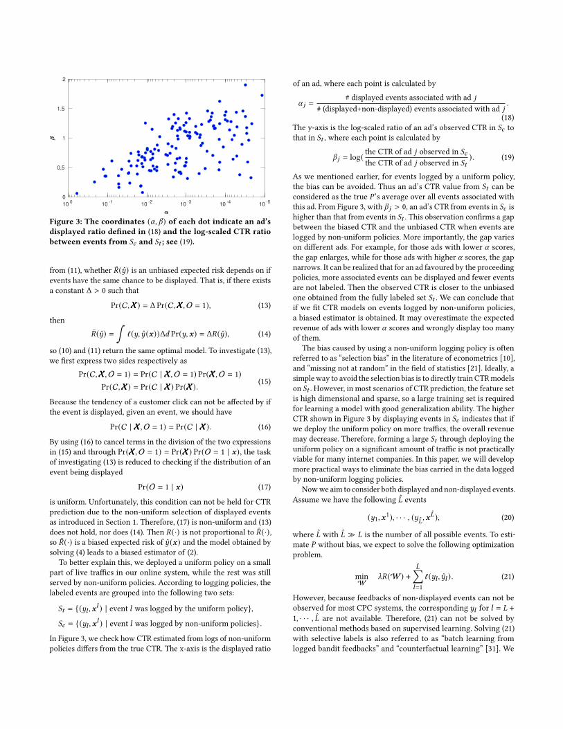
Figure 3: The coordinates (𝛼, 𝛽) of each dot indicate an ad’sdisplayed ratio defined in (18) and the log-scaled CTR ratiobetween events from 𝑆𝑐 and 𝑆𝑡 ; see (19).
from (11), whether 𝑅(𝑦) is an unbiased expected risk depends on if
events have the same chance to be displayed. That is, if there exists
a constant Δ > 0 such that
Pr(C,XXX) = Δ Pr(C,XXX,O = 1), (13)
then
𝑅(𝑦) =∫
ℓ (𝑦,𝑦 (𝒙))Δ𝑑 Pr(𝑦, 𝒙) = Δ𝑅(𝑦), (14)
so (10) and (11) return the same optimal model. To investigate (13),
we first express two sides respectively as
Pr(C,XXX,O = 1) = Pr(C | XXX,O = 1) Pr(XXX,O = 1)Pr(C,XXX) = Pr(C | XXX) Pr(XXX). (15)
Because the tendency of a customer click can not be affected by if
the event is displayed, given an event, we should have
Pr(C | XXX,O = 1) = Pr(C | XXX). (16)
By using (16) to cancel terms in the division of the two expressions
in (15) and through Pr(XXX,O = 1) = Pr(XXX) Pr(O = 1 | 𝒙), the taskof investigating (13) is reduced to checking if the distribution of an
event being displayed
Pr(O = 1 | 𝒙) (17)
is uniform. Unfortunately, this condition can not be held for CTR
prediction due to the non-uniform selection of displayed events
as introduced in Section 1. Therefore, (17) is non-uniform and (13)
does not hold, nor does (14). Then 𝑅(·) is not proportional to 𝑅(·),so 𝑅(·) is a biased expected risk of 𝑦 (𝒙) and the model obtained by
solving (4) leads to a biased estimator of (2).
To better explain this, we deployed a uniform policy on a small
part of live traffics in our online system, while the rest was still
served by non-uniform policies. According to logging policies, the
labeled events are grouped into the following two sets:
𝑆𝑡 = {(𝑦𝑙 , 𝒙𝑙 ) | event 𝑙 was logged by the uniform policy},
𝑆𝑐 = {(𝑦𝑙 , 𝒙𝑙 ) | event 𝑙 was logged by non-uniform policies}.
In Figure 3, we check how CTR estimated from logs of non-uniform
policies differs from the true CTR. The x-axis is the displayed ratio
of an ad, where each point is calculated by
𝛼 𝑗 =# displayed events associated with ad 𝑗
# (displayed+non-displayed) events associated with ad 𝑗.
(18)
The y-axis is the log-scaled ratio of an ad’s observed CTR in 𝑆𝑐 to
that in 𝑆𝑡 , where each point is calculated by
𝛽 𝑗 = log( the CTR of ad 𝑗 observed in 𝑆𝑐
the CTR of ad 𝑗 observed in 𝑆𝑡). (19)
As we mentioned earlier, for events logged by a uniform policy,
the bias can be avoided. Thus an ad’s CTR value from 𝑆𝑡 can be
considered as the true 𝑃 ’s average over all events associated with
this ad. From Figure 3, with 𝛽 𝑗 > 0, an ad’s CTR from events in 𝑆𝑐 is
higher than that from events in 𝑆𝑡 . This observation confirms a gap
between the biased CTR and the unbiased CTR when events are
logged by non-uniform policies. More importantly, the gap varies
on different ads. For example, for those ads with lower 𝛼 scores,
the gap enlarges, while for those ads with higher 𝛼 scores, the gap
narrows. It can be realized that for an ad favoured by the proceeding
policies, more associated events can be displayed and fewer events
are not labeled. Then the observed CTR is closer to the unbiased
one obtained from the fully labeled set 𝑆𝑡 . We can conclude that
if we fit CTR models on events logged by non-uniform policies,
a biased estimator is obtained. It may overestimate the expected
revenue of ads with lower 𝛼 scores and wrongly display too many
of them.
The bias caused by using a non-uniform logging policy is often
referred to as “selection bias” in the literature of econometrics [10],
and “missing not at random” in the field of statistics [21]. Ideally, a
simpleway to avoid the selection bias is to directly train CTRmodels
on 𝑆𝑡 . However, in most scenarios of CTR prediction, the feature set
is high dimensional and sparse, so a large training set is required
for learning a model with good generalization ability. The higher
CTR shown in Figure 3 by displaying events in 𝑆𝑐 indicates that if
we deploy the uniform policy on more traffics, the overall revenue
may decrease. Therefore, forming a large 𝑆𝑡 through deploying the
uniform policy on a significant amount of traffic is not practically
viable for many internet companies. In this paper, we will develop
more practical ways to eliminate the bias carried in the data logged
by non-uniform logging policies.
Nowwe aim to consider both displayed and non-displayed events.
Assume we have the following �̂� events
(𝑦1, 𝒙1), · · · , (𝑦
�̂�, 𝒙�̂�), (20)
where �̂� with �̂� ≫ 𝐿 is the number of all possible events. To esti-
mate 𝑃 without bias, we expect to solve the following optimization
problem.
min
W_𝑅(W) +
�̂�∑𝑙=1
ℓ (𝑦𝑙 , 𝑦𝑙 ). (21)
However, because feedbacks of non-displayed events can not be
observed for most CPC systems, the corresponding 𝑦𝑙 for 𝑙 = 𝐿 +1, · · · , �̂� are not available. Therefore, (21) can not be solved by
conventional methods based on supervised learning. Solving (21)
with selective labels is also referred to as “batch learning from
logged bandit feedbacks” and “counterfactual learning” [31]. We

give a brief review of existing approaches on this topic in the next
section.
3 EXISTING APPROACHES FOR LEARNINGFROM SELECTIVE LABELS
Existing approaches for solving (21) with selective labels broadly
fall into the following three categories: direct method, the inverse-
propensity-scoring method, and the doubly robust method.
3.1 Direct MethodAs we mentioned above, the key challenge in solving (21) is that we
lack labels of those non-displayed events. Direct methods are based
on an intuitive idea that we can find a relationship 𝜎 (·) betweenlabels and features of displayed events such that 𝜎 (𝒙𝑙 ) ≈ 𝑦𝑙 , for
𝑙 = 1, · · · , 𝐿. We call 𝜎 (·) as an imputation model, which can impute
labels for all events and have the following �̂� labeled samples
(𝜎1, 𝒙1), · · · , (𝜎
�̂�, 𝒙�̂�),
where 𝜎𝑙 ≡ 𝜎 (𝒙𝑙 ). Then we solve the following standard supervisedlearning problem.
min
W_𝑅(W) +
�̂�∑𝑙=1
ℓ (𝜎𝑙 , 𝑦𝑙 ) . (22)
Clearly, the performance of a direct method is determined by the
quality of 𝜎 (·). Many past works found 𝜎 (·) via conductingmachine
learning techniques on the labeled data set. For example, ridge linear
regression [6], and random forests [19] are considered.
3.2 Inverse-Propensity-Scoring (IPS) MethodBy assuming the logging policy is stochastic, the IPS method pro-
posed in [11] weights each labeled event with the inverse of its
propensity score, which refers to the tendency or the likelihood
of an event being logged. Specifically, given the event 𝑙 , we can
observe an indicator 𝑂𝑙 ∈ {0, 1}, which indicates if the event was
displayed. Following [30, 32], we assume that 𝑂𝑙 is sampled from a
Bernoulli distribution as 𝑂𝑙 ∼ Bern(𝑧𝑙 ), where 𝑧𝑙 is the probabilityof the event being displayed. Here we consider 𝑧𝑙 as the propensity
scores of event 𝑙 . The IPS method solves the following problem.
min
W_𝑅(W) +
�̂�∑𝑙=1
ℓ (𝑦𝑙 , 𝑦𝑙 )𝑧𝑙
𝑂𝑙 ,
which, according to the observations of 𝑂𝑙 , ∀𝑙 , is equivalent to
min
W_𝑅(W) +
𝐿∑𝑙=1
ℓ (𝑦𝑙 , 𝑦𝑙 )𝑧𝑙
. (23)
The following proof has been given in past works, which shows
that solving (23) can get an unbiased estimator of 𝑃 .
E𝑂 [�̂�∑𝑙=1
ℓ (𝑦𝑙 , 𝑦𝑙 )𝑧𝑙
𝑂𝑙 ] =�̂�∑𝑙=1
ℓ (𝑦𝑙 , 𝑦𝑙 )𝑧𝑙
· E𝑂 [𝑂𝑙 ] = (21).
Before solving (23), we need to know 𝑧𝑙 for 𝑙 = 1, · · · , 𝐿. Thework[30] differentiates two settings for the assignment mechanism of 𝑧𝑙 .
The first is an experimental setting, where any event 𝑧𝑙 is decided
by us and𝑂𝑙 is generated according to 𝑧𝑙 . Therefore we can directly
solve (23) with known 𝑧𝑙 . Many past works and data sets (e.g.,
[20, 31]) are based on this setting. The second is an observational
setting, where𝑂𝑙 is not controlled by us, so 𝑧𝑙 is implicit. In this case,
we must estimate 𝑧𝑙 first by some techniques. For example, naive
Bayes [30], survival models [37], and more generally, by assigning
𝑂𝑙 =
{1 the event was displayed,
0 the event was not displayed,
we can find a relationship 𝑜 (·) between 𝑂𝑙 and the given features
such that 𝑜 (𝒙𝑙 ) ≈ 𝑂𝑙 , for 𝑙 = 1, · · · , �̂� by any machine learning
techniques (e.g., logistic regression [30], gradient boosting [25]).
Then 𝑧𝑙 ≡ 𝑜 (𝒙𝑙 ) for 𝑙 = 1, · · · , 𝐿 can be used as the propensity
scores in (23).
3.3 Doubly Robust MethodDoubly robust method for counterfactual learning was first pro-
posed in [6], which takes advantage of the two aforementioned
approaches by combining them together. Therefore, the following
optimization problem is solved.
min
W_𝑅(W)+
𝐿∑𝑙=1
( ℓ (𝑦𝑙 , 𝑦𝑙 )𝑧𝑙
− ℓ (𝜎𝑙 , 𝑦𝑙 ))
︸ ︷︷ ︸IPS method part
+�̂�∑𝑙=1
ℓ (𝜎𝑙 , 𝑦𝑙 )︸ ︷︷ ︸direct method part
. (24)
The analysis in [6] shows that the bias of the doubly robust method
is the product of the two parts from the direct method and the IPS
method. Therefore, the bias of the doubly robust method can be
eliminated if either the direct method part or the IPS method part is
unbiased. Empirical studies confirm that the doubly robust method
performs better than solely a direct method or an IPS method.
3.4 Discussion on Feasibility of ExistingApproaches for CPC Systems
Though the estimators obtained by above-mentioned methods are
expected to give unbiased predictions of 𝑃 , we show that there
exist three main obstacles for applying these approaches for CTR
prediction in a real-world CPC system.
First, from the theoretic guarantee established by past literatures,
IPS works when the logging policy is stochastic such that with the
increase of 𝐿, sufficient events with various propensity scores can be
observed. That is, though the policy tends to select the events with
high propensity scores, those with low propensity scores still can
have a chance to be displayed and included in the labeled set. For
events with low propensity scores, the formulation in (23) leads to
larger corresponding instance weights, and then IPS can correct the
selection bias. However, commercial products such as CPC systems
usually avoid a stochastic policy because of the risk of revenue loss.
Instead, as we introduced in Section 1, the policy makes decisions
by considering if the expected revenue is large enough. Therefore,
the logging policy of our CPC system can be considered as under
the following deterministic setting.
𝑂𝑙 = I(ECPM𝑙 > 𝑡), (25)
where ECPM𝑙 is the expected revenue of the event 𝑙 , and 𝑡 is a
dynamic threshold. This policy deterministically selects the events
with high propensity scores to be displayed. In this case, the events

with low propensity scores are absent in the labeled set. The de-
terministic logging policy makes theory and practice of the IPS
method inapplicable to practical CTR prediction.
Secondly, for the direct method and the corresponding part in
the doubly robust method, we need an imputation model 𝜎 (·) togenerate labels for non-displayed events. However, as we have
shown that displayed events may carry the selection bias in Sec-
tion 2.2, many existing works [6, 19] find that imputation models
learnt from displayed events will propagate the selection bias to the
non-displayed events. Then both the direct and the doubly robust
methods cannot give unbiased predictions.
The third issue is that for estimators obtained by solving opti-
mization problems like (22) and (24), they involveO(�̂�) costs of time
and space. However, �̂� is extremely large considering all displayed
and non-displayed events. Therefore, to have a practical framework
for large-scale counterfactual CTR prediction, any O(�̂�) cost ofstorage and computation should be avoided.
4 A PRACTICAL FRAMEWORK FORCOUNTERFACTUAL CTR PREDICTION
To address issues mentioned in Section 3.4, we propose a practical
framework for counterfactual CTR prediction. Our framework ex-
tends the doubly robust method by dropping the propensity scores
to address the issue of using a deterministic logging policy. We call
it as the propensity-free doubly robust method. To further improve
the robustness of our framework, we propose a new way to obtain
the imputation model by taking the advantage of the small but
unbiased set 𝑆𝑡 defined in Section 2.2. Finally, by connecting the
CTR prediction with recommender systems, we propose an efficient
training algorithm so that the prohibitive O(�̂�) cost can be trickily
avoided if some conditions are satisfied.
4.1 Propensity-free Doubly Robust MethodA recent work [19] describes an analogous scenario that many
commercial statistical machine translation systems only determin-
istically provide the best translation result to users and then collect
corresponding feedbacks. Then they find that in their scenario, the
doubly robust method still can perform well even under a deter-
ministic logging policy. Their analysis provides a reason behind the
result that the direct method part of doubly robust imputes labels
for non-displayed events, which remedies the absence of unlabeled
events and improves the generalization ability of the model. This
result motivates us to investigate if the similar idea can be extended
on CTR prediction. Specifically, we follow [19] to set 𝑧𝑙 = 1 for all
displayed events logged by a deterministic policy. Then we modify
(24) to have the following problem of the propensity-free doubly
robust method.
min
W_𝑅(W) +
𝐿∑𝑙=1
(ℓ (𝑦𝑙 , 𝑦𝑙 ) −𝜔ℓ (𝜎𝑙 , 𝑦𝑙 )
)+𝜔
�̂�∑𝑙=1
ℓ (𝜎𝑙 , 𝑦𝑙 ), (26)
where 𝜔 is used as a hyper-parameter to balance the IPS part and
the direct method part.
Recall that the concept of the doubly robust method is that the
bias can be eliminated if either one of the two sub-estimators is
unbiased. Compared with (24), we can see that the IPS part in (26)
under the setting of 𝑧𝑙 = 1 is essentially reduced to the naive binary
Unbiased
Set 𝑆𝑡
Imputation
Model 𝜎 (·)
Displayed
𝑆𝑐 ∪ 𝑆𝑡
Non-displayed
All events
CTR
Model 𝑦 (·)
Uniform
Policy
Learned from
𝑆𝑡
Non-uniform
Policies
Imputing
Labels
Propensity-free
Doubly Robust
Figure 4: A diagram showing components of our framework
classification problem (4), which definitely cannot give unbiased
predictions. Therefore, we rely on the direct method part to get unbi-
ased predictions. However, if we follow existing works of the doubly
robust method (e.g., [6, 19]) to learn 𝜎 (·) from displayed events, the
carried selection bias will be propagated to non-displayed events
through the imputation model. In this case, the direct method part
can not give unbiased predictions either. In order to avoid this situ-
ation, we design a new approach to obtain the imputation model in
the next section.
4.2 Unbiased Imputation ModelsRecall that in Section 2.2, to help realize the severity of the selection
bias, we collect a labeled set 𝑆𝑡 through deploying a uniform policy
on a small percentage of our online traffic. Though 𝑆𝑡 is very small,
it still contains some gold-standard unbiased information. We aim
to leverage 𝑆𝑡 in our framework.
Past studies that have used 𝑆𝑡 include, for example, [3, 29]. By
considering both 𝑆𝑐 and 𝑆𝑡 as training sets, they jointly learn two
models respectively from the two sets in a multi-task fashion and
conduct predictions by combining the two models. Our approach
differs from theirs on the usage of 𝑆𝑡 . As illustrated in Figure 4, we
learn the imputation model 𝜎 (·) from 𝑆𝑡 and apply the model to
impute labels of all displayed and non-displayed events; see the last
term in (26).
Note that in our framework, learning the imputation model and
learning the CTR model are two separate tasks. Different from the
task of learning the CTR model which is generally complex and
requires a large training set, the task of learning the imputation
model is much more flexible. We can decide the imputation model
and the corresponding feature set depending on the size of 𝑆𝑡 . That
is, when 𝑆𝑡 is large enough, the task can be as complex as that of
learning the CTR model. But when the size of 𝑆𝑡 is limited, the task
can be reduced to impute labels with a single value inferred from
𝑆𝑡 (e.g., the average CTR in 𝑆𝑡 ). Through the experimental results
shown in Section 5.5, we will see that unbiased imputation models
help our framework to obtain good performances even if 𝑆𝑡 is very
small.
4.3 Efficient TrainingBy imputing labels for all possible events in the direct method part,
(26) becomes a standard classification problem with �̂� instances.
Because �̂� can be extremely large for a real-world CPC system, any
cost of O(�̂�) will make the training process infeasible. Therefore,

many existing optimization techniques, if directly applied, are un-
able to efficiently solve (26). For example, the stochastic gradient
(SG) method popularly used for CTR prediction [8, 16] may face
difficulties in the process of sampling O(�̂�) instances.2 To overcome
the difficulties, we connect CPC systems with a related but different
field, called recommender systems, where an analogous issue has
been well-studied.
In a typical recommender system, we observe part of a rating
matrix 𝑌 ∈ R𝑚×𝑛 of𝑚 users and 𝑛 items. For each observed (𝑖, 𝑗)pair, 𝑌𝑖 𝑗 indicates the rating of item 𝑗 given by user 𝑖 . The goal is to
predict the rating of an item not rated by a user yet. Following the
idea, if we consider an event as a (request, ad) pair, an advertising
system is naturally a recommender system. As illustrated in Figure
5, the 𝐿 displayed events can be considered as 𝐿 observed (request,
ad) entries in a rating matrix 𝑌 ∈ R𝑚×𝑛 , where 𝑚 is the total
number of requests and 𝑛 is the total number of ads. According
to whether the ad was clicked by the user or not, these observed
entries can be grouped into the following two sets
Ω+ = {(𝑖, 𝑗) | ad 𝑗 was displayed and clicked in request 𝑖},Ω− = {(𝑖, 𝑗) | ad 𝑗 was displayed but not clicked in request 𝑖}.
By assigning ratings to observed entries as
𝑌𝑖 𝑗 =
{1 (𝑖, 𝑗) ∈ Ω+,−1 (𝑖, 𝑗) ∈ Ω−,
and replacing the index 𝑙 with the index (𝑖, 𝑗), we can re-write (26)
as
min
W_𝑅(W) +
∑(𝑖, 𝑗) ∈Ω
(ℓ (𝑌𝑖 𝑗 , 𝑌𝑖 𝑗 ) − 𝜔ℓ (𝐴𝑖 𝑗 , 𝑌𝑖 𝑗 )
)+ 𝜔
𝑚∑𝑖=1
𝑛∑𝑗=1
ℓ (𝐴𝑖 𝑗 , 𝑌𝑖 𝑗 ),(27)
where
Ω = Ω+ ∪ Ω−
is the set of displayed pairs with |Ω | = 𝐿, �̂� =𝑚𝑛, 𝑌 ∈ R𝑚×𝑛 is the
output matrix with 𝑌𝑖 𝑗 = 𝑦 (𝒙𝑖, 𝑗 ), and 𝐴 ∈ R𝑚×𝑛 is the matrix of
imputed labels with
𝐴𝑖 𝑗 = 𝜎 (𝒙𝑖, 𝑗 ) . (28)
Under the above setting, �̂� = 𝑚𝑛 indicates the total number of
possible events. The second term in (27) involves O(𝑚𝑛) = O(�̂�)operations, which are prohibitive when𝑚 and 𝑛 are large. The same
O(𝑚𝑛) difficulty occurs in a topic called “recommender systems
with implicit feedbacks” [12, 13, 33, 36]. It describes a scenario
where a rating matrix 𝑌 includes both positive and negative entries.
However, only a subset Ω+ including some positive entries have
been observed. An approach to handle this scenario is to treat all
unobserved pairs as a negative rating 𝑟 , such as 0 or -1 in [34, 36].
Let 𝐴 ∈ R𝑚×𝑛 be an artificial rating matrix with
𝐴𝑖 𝑗 =
{1 (𝑖, 𝑗) ∈ Ω+,𝑟 (𝑖, 𝑗) ∉ Ω+ .
(29)
2The failure of SG on handling similar scenarios has been reported in several past
works [33, 36].
ad 1 ad 2 · · · · · · ad 𝑛
request 1
.
.
.
request𝑚
✓ ✗ ? ? ?
? ? ? ✓ ✗
? ✓ ? ? ✗
Figure 5: An illustration of a rating matrix of 𝑚 requestsand 𝑛 ads, where 𝐿 events are displayed. The symbols ‘✓’, ‘✗’,and ‘?’ indicate the event is clicked, not clicked, and not dis-played, respectively.
To find a model fitting all 𝐴𝑖 𝑗 values, the cost of O(𝑚𝑛) arises insolving the following problem with𝑚𝑛 instances.
min
W_𝑅(W) +
𝑚∑𝑖=1
𝑛∑𝑗=1
𝐶𝑖 𝑗 ℓ (𝐴𝑖 𝑗 , 𝑌𝑖 𝑗 ) . (30)
where 𝐶𝑖 𝑗 is a cost parameter. To avoid the O(𝑚𝑛) cost, existingstudies [1, 33, 34, 36] impose some resctrictions on terms over values
not in Ω+ and change (30) to
min
W_𝑅(W) +
∑(𝑖, 𝑗) ∈Ω+
𝐶𝑖 𝑗 ℓ (1, 𝑌𝑖 𝑗 ) +∑(𝑖, 𝑗)∉Ω+
𝐶𝑖 𝑗 ℓ̄ (𝑟, 𝑌𝑖 𝑗 )
=_𝑅(W) +∑(𝑖, 𝑗) ∈Ω+
(𝐶𝑖 𝑗 ℓ (1, 𝑌𝑖 𝑗 ) −𝐶𝑖 𝑗 ℓ̄ (𝑟, 𝑌𝑖 𝑗 )
)+
𝑚∑𝑖=1
𝑛∑𝑗=1
𝐶𝑖 𝑗 ℓ̄ (𝑟, 𝑌𝑖 𝑗 ), (31)
where the following conditions should apply.
• The cost parameters 𝐶𝑖 𝑗 in (31) cannot be arbitrary values. In
practice, a constant value is often considered.
• A simple loss function ℓ̄ (·, ·) is needed. In most existing works
the squared loss is considered.
• The model function 𝑦 (·) can not be an arbitrary one. Specifically,
given a feature vector 𝒙𝑖, 𝑗 , 𝑦 (𝒙𝑖, 𝑗 ) can be factorized into multiple
parts, each of which is only related to 𝑖 or 𝑗 and convex in the
corresponding parameters. For example, a modified FFM model
proposed in [36] satisfies this condition.
Optimization methods have been proposed so that the O(𝑚𝑛) termin the overall cost can be replaced with a smaller O(𝑚) +O(𝑛) term.
The main reason why O(𝑚𝑛) can be eliminated is because results
on all 𝑖 and all 𝑗 can be obtained by using values solely related to
𝑖 and 𝑗 , respectively. A conceptual illustration is in the following
equation.
𝑚∑𝑖=1
𝑛∑𝑗=1
(· · · ) =𝑚∑𝑖=1
(· · · ) × or +𝑛∑𝑗=1
(· · · ). (32)
By considering the similarity between (27) and (31), with the
corresponding restrictions in mind, we propose the following final

realization of the framework (26):
min
W_𝑅(W) +
∑(𝑖, 𝑗) ∈Ω
(ℓ (𝑌𝑖 𝑗 , 𝑌𝑖 𝑗 ) − 𝜔 (𝐴𝑖 𝑗 − 𝑌𝑖 𝑗 )2
)+ 𝜔
𝑚∑𝑖=1
𝑛∑𝑗=1
(𝐴𝑖 𝑗 − 𝑌𝑖 𝑗 )2 .(33)
For (𝑖, 𝑗) in Ω, we allow general convex loss functions in the original
IPS part to maintain the connection to conventional CTR training,
while in the direct method part, we follow the above restriction for
ℓ̄ in (31) to consider the squared loss. We then compare the two
O(𝑚𝑛) terms in (31) and (33). By respectively excluding 𝐶𝑖 𝑗 and 𝜔 ,
ours considers a more complicated setting of 𝐴 in (28), where all
𝑚𝑛 entries can be various rather than only a constant value in (31).
There remains a cost of O(𝑚𝑛) caused by 𝐴 in (33). Inspired by
the restriction of 𝑦 (·) that is used to have 𝑌𝑖 𝑗 = 𝑦 (𝒙𝑖, 𝑗 ), to extendexisting optimization methods for (31) on our proposed framework,
an additional condition should be considered:
• The imputation model function 𝜎 (·) can not be an arbitrary one.
Specifically, given a feature vector 𝒙𝑖, 𝑗 , 𝜎 (𝒙𝑖, 𝑗 ) can be factorized
into multiple parts, each of which is only related to 𝑖 or 𝑗 but
not required to be convex in parameters. Thus the choice of 𝜎 (·)is broader than that of 𝑦 (·). For example, the multi-view deep
learning approach proposed in [7] satisfies this condition.
In our realization, we implement various imputation models from
simple to complex, all of which satisfy the above condition; see
details in Section 5.2.2.
To use (33), we consider the FFM model for 𝑦 (𝒙𝑖, 𝑗 ) and develop
an optimization method. Details are in Section A of supplementary
materials.
5 EXPERIMENTSWe begin by presenting our experimental settings including data
sets and parameter selections. Then, we design and conduct a series
of experiments to demonstrate the effectiveness and robustness of
our proposed framework in Section 4.
5.1 Data SetsWe consider the following data sets for experiments, where statistics
are described in Table 2.
• CPC: This is a large-scale data set for CTR prediction, which
includes events of nine days from a real-world CPC system. We
consider a two-slot scenario so that for each request, the two
ads with the highest expected revenues from 140 candidates
are displayed. To have training, validation and test sets under
uniform and non-uniform policies, as illustrated in Figure 6, we
segment the data to six subsets. The five subsets used in our
experiments are described below.
– 𝑆𝑡 , 𝑆𝑐 defined in Section 2.2, are used separately or together as
the training set depending the approach.
– 𝑆va is the set obtained in the validation period under the uni-
form logging policy. As an unbiased set, it is used by all meth-
ods for the parameter selection.
– 𝑆te is the set obtained in the test period under the uniform
logging policy. As an unbiased set, it is used to check the test
performance of all methods.
Non-uniform
policies:
𝑆𝑐 𝑆 ′𝑐
Uniform
policy:
𝑆𝑡 𝑆va 𝑆te
1 2 3—9
days
Figure 6: An illustration of data segmentation according totraining, validation, and test periods.
Table 2: Data statistics
Data set 𝑚 𝑛 𝐷 |𝑆𝑐 | |𝑆𝑡 | |𝑆va | |𝑆te |Yahoo! R3 14,877 1,000 15,877 176,816 2,631 2,775 48,594
CPC 21.7M 140 1.4M 42.8M 0.35M 0.31M 2.0M
– 𝑆 ′𝑐 is the set of events logged by non-uniform policies in the
validation period. For methods that have involved 𝑆𝑐 for train-
ing in the validation process, after parameters are selected, 𝑆 ′𝑐is included for training the final model to predict 𝑆te.
For the feature set, we collect user profiles, contextual informa-
tion (e.g., time, location) of each request and side information of
each advertisement. All are categorical features.
• Yahoo! R3 [23]: The data set, from a music recommendation ser-
vice, includes a training and a test set of rated (user, song) pairs in
a rating matrix 𝑅. For the training set, users deliberately selected
and rated the songs by preference, which can be considered as
a stochastic logging policy by following [30, 32]. For the test
set, users were asked to rate 10 songs randomly selected by the
system. Because the logging policy of the test set is completely
random, the ratings contained in the test set can be considered
as the ground truth without the selection bias. In Section B.1 of
supplementary material, we give details of modifying the prob-
lem to simulate a deterministic logging policy, which is what our
framework intends to handle.
5.2 Considered ApproachesThe considered approaches in our comparison fall into two main
categories.
5.2.1 Conventional Approaches for CTR Prediction. This categoryincludes approaches that solve the binary classification problem in
(4) with the following CTR model.
• FFM: This is the CTR model reviewed in Section 2.1. We consider
the slightly modified formulation proposed in [36].
For the training set, we consider the following three combinations
of 𝑆𝑐 and 𝑆𝑡 .
• 𝑆𝑐 : This is a large set including events logged by non-uniform
policies; see Section 2.2. This simulates the setting of most sys-
tems for CTR prediction.
• 𝑆𝑡 : This is a small set including events logged by a uniform policy;
see Section 2.2. Because the set is free from the selection bias,
some works (e.g., [22]) deploy a model trained on 𝑆𝑡 , though an
issue is that |𝑆𝑡 | is small.
• 𝑆𝑐 ∪ 𝑆𝑡 : This is the set of all logged events.

5.2.2 Counterfactual Learning Approaches. This category includes
the following approaches, where all of them consider FFM as the
CTR model and 𝑆𝑐 ∪ 𝑆𝑡 as the training set.
• IPS: The approach was reviewed in Section 3.2. For the estimation
of propensity scores, we follow [30] to consider the following
Naive Bayes propensity estimator.
𝑧𝑙 ≈ 𝑃 (𝑂𝑙 = 1 | 𝑦𝑙 = 𝑦) ≈ 𝑃 (𝑦,𝑂 = 1)𝑃 (𝑦) , (34)
where 𝑦 = {−1, 1} is the label, 𝑃 (𝑦,𝑂 = 1) is the ratio of events
labeled as𝑦 in the displayed set, and 𝑃 (𝑦) is the ratio of the eventslabeled as 𝑦 in a selection-bias free set. We estimated them by
respectively using 𝑆𝑐 ∪ 𝑆𝑡 and 𝑆𝑡 .• CausE: The “causal embedding” approach [3] jointly learns two
CTR models 𝑦𝑐 (·) and 𝑦𝑡 (·) respectively from 𝑆𝑐 and 𝑆𝑡 . They
solve the following optimization problem.
min
W𝑐 ,W𝑡
1
|𝑆𝑐 |∑
(𝑦,𝒙) ∈𝑆𝑐ℓ (𝑦,𝑦𝑐 (𝒙)) +
1
|𝑆𝑡 |∑
(𝑦,𝒙) ∈𝑆𝑡ℓ (𝑦,𝑦𝑡 (𝒙))
+ _𝑐𝑅(W𝑐 ) + _𝑡𝑅(W𝑡 ) + _ ∥𝑡−𝑐 ∥ ∥W𝑐 −W𝑡 ∥22 ,
whereW𝑐 andW𝑡 are are parameters of 𝑦𝑐 (·) and 𝑦𝑡 (·), respec-tively, and the last term controls the discrepancy betweenW𝑐
andW𝑡 . The original study in [3] only supports matrix factor-
ization models. We make an extension to support more complex
models (e.g., FFM). For the prediction, we follow [3] to use only
𝑦𝑐 (·).• New: This approach is a realization of our proposed framework
in (33), where we use the logistic loss defined in (5) as ℓ (·, ·). We
use a modified FFM model in [36] for the CTR model 𝑦 (·). Itsatisfies the conditions needed in Section 4.3. For the imputation
model 𝜎 (·), we consider three settings.– avg: This is a simple setting is to impute labels with the
average CTR in 𝑆𝑡 . We use the following logit function to
transform a probability to a model output in [−∞,∞].
𝜎 (𝒙𝑖, 𝑗 ) = log( CTR
1 − CTR), ∀𝑖, 𝑗
where CTR is the average CTR from events in 𝑆𝑡 .
– item-avg: This is an item-wise extension of avg as
𝜎 (𝒙𝑖, 𝑗 ) = log(CTR𝑗
1 − CTR 𝑗
), ∀𝑖
where CTR𝑗 is the average CTR of ad 𝑗 from events in 𝑆𝑡 .
– complex: This is a complex setting to learn 𝜎 (·) from 𝑆𝑡 by
solving (4) with the modified FFM model in [36].
We further include two constant predictors as baselines.
• average (𝑆𝑐 ): This is a constant predictor defined as
𝑦 (𝒙𝑖, 𝑗 ) = log( CTR
1 − CTR), ∀𝑖, 𝑗
where CTR is the average CTR from events in 𝑆𝑐 .
• average (𝑆𝑡 ): It is the same as average (𝑆𝑐 ), except that the averageCTR from events in 𝑆𝑡 is considered.
Table 3: A performance comparison of different approaches.We show the relative improvements over the average (𝑆𝑐 ) ontest NLL and AUC scores. The best approach is bold-faced.
Metric NLL AUC NLL AUC
Approach
Data set Yahoo! R3 CPC
average (𝑆𝑐 ) +0.0% +0.0% +0.0% +0.0%
average (𝑆𝑡 ) +79.1% +0.0% +29.6% +0.0%
FFM (𝑆𝑐 ) -7.7% +36.4% -16.9% +32.2%
FFM (𝑆𝑡 ) -20.7% +4.6% +32.4% +42.8%
FFM (𝑆𝑐 ∪ 𝑆𝑡 ) +0.2% +36.4% +10.6% +34.6%
IPS +62.2% +23.2% +28.5% +31.2%
CausE +6.8% +37.8% +25.3% +39.4%
New (avg) +79.1% +51.8% +32.9% +48.6%
New (item-avg) +76.8% +54.2% +32.4% +48.2%
New (complex) -0.2% +37.4% +33.4% +50.6%
Table 4: The performance when 𝑆𝑡 becomes smaller sets. |𝑆𝑡 |indicates the size of 𝑆𝑡 as the percentage of total data. Wepresent the relative improvements over the average (𝑆𝑐 ) ontest NLL and AUC scores. The CPC set is considered and thebest approach is bold-faced.
Metric NLL AUC NLL AUC
Approach
|𝑆𝑡 |0.1% 0.01%
average (𝑆𝑡 ) +29.2% +0.0% +28.7% +0.0%
FFM (𝑆𝑡 ) +28.6% +18.6% +26.5% +1.2%
FFM (𝑆𝑐 ∪ 𝑆𝑡 ) -12.5% +29.6% -16.9% +32.0%
IPS +26.1% +26.8% +18.7% +23.6%
CausE +25.6% +37.4% +22.4% +31.6%
New (avg) +33.5% +48.4% +30.4% +47.2%New (item-avg) +31.5% +46.6% +26.7% +46.0%
New (complex) +32.2% +44.6% +32.5% +43.0%
For evaluation criteria, we consider NLL and AUC respectively
defined in (8) and (9) and report relative improvements over the
method average (𝑆𝑐 ) as
𝑐𝑟𝑖𝑡𝑒𝑟𝑖𝑜𝑛𝑎𝑝𝑝𝑟𝑜𝑎𝑐ℎ − 𝑐𝑟𝑖𝑡𝑒𝑟𝑖𝑜𝑛average (𝑆𝑐 )|𝑐𝑟𝑖𝑡𝑒𝑟𝑖𝑜𝑛average (𝑆𝑐 ) |
,
where 𝑐𝑟𝑖𝑡𝑒𝑟𝑖𝑜𝑛 is either NLL or AUC, and 𝑎𝑝𝑝𝑟𝑜𝑎𝑐ℎ is the ap-
proach being measured. Because the performance of average (𝑆𝑐 ) isunchanged in all experiments, results presented in different tables
can be comparable. Details of our parameter selection procedure
are in supplementary materials.
5.3 Comparison on Various ApproachesBy comparing models in Table 3, we have the following observa-
tions.
• For two constant predictors, NLL scores of average (𝑆𝑡 ) are much
better than those of average (𝑆𝑐 ) estimated from the biased 𝑆𝑐 set.
The reason is that the distribution of 𝑆𝑡 is consistent with that
of the test set. However, because average (𝑆𝑡 ) is still a constantpredictor, its AUC scores are the same as those of average (𝑆𝑐 ).

• For FFM (𝑆𝑡 ), it performs much better than FFM (𝑆𝑐 ) and FFM(𝑆𝑐 ∪ 𝑆𝑡 ) on CPC set. This result confirms our conjecture in Sec-
tion 2.2 that conventional approaches considering only displayed
events selected by non-uniform policies may cause a strong se-
lection bias. However, the result of FFM (𝑆𝑡 ) on Yahoo! R3 set
is not ideal. The reason is that the feature set of Yahoo! R3 is
too sparse by having only two identifier features3and 𝑆𝑡 is too
small to learn an FFM model.
• IPS has good NLL scores, but its AUC scores are not competitive.
In (34) to estimate propensity scores, the set 𝑆𝑡 is used. This
may explain why the obtained NLL is similar to that by average(𝑆𝑡 ). On the other hand, the unsatisfactory AUC results may be
because the Naive Bayes estimator used in (34) is too simple.
• For CausE, it performs better than FFM (𝑆𝑐 ) and FFM (𝑆𝑐 ∪ 𝑆𝑡 )but worse than FFM (𝑆𝑡 ) on the CPC set. The reason might be
that models learnt from 𝑆𝑡 are better than those learnt from 𝑆𝑐 ,
but we follow [3] to use only 𝑦𝑐 (·) for prediction.• Our proposed framework performs significantly better than oth-
ers, though an exception is New (complex) on the Yahoo! R3set. The reason is analogous to the explanation of the bad result
of FFM (𝑆𝑡 ) on Yahoo! R3 set where 𝑆𝑡 is too small. In contrast,
for the CPC set, because 𝑆𝑡 is large enough to learn a complex
imputation model, New (complex) performs the best.
5.4 Impact of Unbiased Imputation ModelsLearnt from 𝑆𝑡
In Section 4.2, we proposed unbiased imputation models because
past works [6, 19] find that learning from biased data sets will propa-
gate the carried selection bias to non-displayed events and worsens
the performance. We conduct an experiment to verify this conjec-
ture and the importance of using an unbiased imputation model.
Detailed results are in Section B.3 of supplementary materials.
5.5 Impact of the Size of 𝑆𝑡To examine the robustness of the approaches relying on 𝑆𝑡 to learn
an unbiased imputation model, we shrink 𝑆𝑡 to see how they per-
form on the CPC set. For experiments in Section 5.3, 𝑆𝑡 includes
1% of the data. We now select two subsets respectively having 0.1%
and 0.01% of total data. These subsets are then used as 𝑆𝑡 for exper-
iments, though each model’s parameters must be re-selected. The
set 𝑆𝑐 remains unchanged.
The result is in Table 4. By comparing the third column of Table 3,
which shows the result of using 1% data as 𝑆𝑡 , we observe that with
the shrinkage of 𝑆𝑡 , the performance of all approaches gradually
becomes worse. However, our proposed framework still performs
significantly better than others. In particular, for other approaches
AUC values are strongly affected by the size of 𝑆𝑡 , but ours remain
similar. Among the three settings of our framework, the simple
setting New (avg) of using average CTR in 𝑆𝑡 as the imputation
model is competitive. This might be because for small 𝑆𝑡 , training
a complicated imputation model is not easy.
3See details of the Yahoo! R3 set in supplementary materials
6 CONCLUSIONIn this work, through an A/B test on our system, we show that
conventional approaches for CTR prediction considering only dis-
played events may cause a strong selection bias and inaccurate
predictions. To alleviate the bias, we need to conduct counterfac-
tual learning by considering non-displayed events. We point out
some difficulties for applying counterfactual learning techniques
in real-world advertising systems.
(1) For many advertising systems, the thresholding operation (25)
is applied as a deterministic logging policy, but existing ap-
proaches may require stochastic policies.
(2) Learning imputation models from displayed events causes the
selection bias being propagated to non-displayed events.
(3) The high cost of handling all displayed and non-displayed
events causes some approaches impractical for large systems.
To overcome these difficulties, we propose a novel framework for
counterfactual CTR prediction. We introduce a propensity-free dou-
bly robust method. Then we propose a setting to obtain unbiased
imputation models in our framework. For efficient training we
link the proposed framework to recommender systems with im-
plicit feedbacks and adapt algorithms developed there. Experiments
conducted on real-world data sets show our proposed framework
outperforms not only conventional approaches for CTR prediction
but also some existing counterfactual learning methods.
REFERENCES[1] Immanuel Bayer, Xiangnan He, Bhargav Kanagal, and Steffen Rendle. 2017. A
generic coordinate descent framework for learning from implicit feedback. In
WWW.
[2] Mathieu Blondel, Masakazu Ishihata, Akinori Fujino, and Naonori Ueda. 2016.
Polynomial Networks and Factorization Machines: new Insights and Efficient
Training Algorithms. In ICML.[3] Stephen Bonner and Flavian Vasile. 2018. Causal Embeddings for Recommenda-
tion. In RecSys.[4] Olivier Chapelle, Eren Manavoglu, and Romer Rosales. 2015. Simple and scalable
response prediction for display advertising. ACM TIST 5, 4 (2015), 61:1–61:34.
[5] Wei-Sheng Chin, Bo-Wen Yuan, Meng-Yuan Yang, and Chih-Jen Lin. 2018. An
Efficient Alternating Newton Method for Learning Factorization Machines. ACMTIST 9 (2018), 72:1–72:31.
[6] Miroslav Dudík, John Langford, and Lihong Li. 2011. Doubly robust policy
evaluation and learning. In ICML.[7] Ali Mamdouh Elkahky, Yang Song, and Xiaodong He. 2015. A multi-view deep
learning approach for cross domain user modeling in recommendation systems.
In WWW.
[8] Huifeng Guo, Ruiming Tang, Yunming Ye, Zhenguo Li, and Xiuqiang He. 2017.
DeepFM: a factorization-machine based neural network for CTR prediction. In
IJCAI.[9] Xinran He, Junfeng Pan, Ou Jin, Tianbing Xu, Bo Liu, Tao Xu, Yanxin Shi, Antoine
Atallah, Ralf Herbrich, Stuart Bowers, and Joaquin Quiñonero Candela. 2014.
Practical Lessons from Predicting Clicks on Ads at Facebook. In ADKDD.[10] James J. Heckman. 1979. Sample selection bias as a specification error. Econo-
metrica 47, 1 (1979), 153–161.[11] Daniel G. Horvitz and Donovan J. Thompson. 1952. A Generalization of Sampling
Without Replacement From a Finite Universe. J. Amer. Statist. Assoc. 47 (1952),663–685.
[12] Cho-Jui Hsieh, Nagarajan Natarajan, and Inderjit Dhillon. 2015. PU Learning for
Matrix Completion. In ICML.[13] Yifan Hu, Yehuda Koren, and Chris Volinsky. 2008. Collaborative filtering for
implicit feedback datasets. In ICDM.
[14] Machael Jahrer, Andreas Töscher, Jeong-Yoon Lee, Jingjing Deng, Hang Zhang,
and Jacob Spoelstra. 2012. Ensemble of Collaborative Filtering and Feature
EngineeredModel for Click Through Rate Prediction. InKDDCup 2012Workshop.[15] Yuchin Juan, Damien Lefortier, and Olivier Chapelle. 2017. Field-aware factoriza-
tion machines in a real-world online advertising system. In WWW.
[16] Yuchin Juan, Yong Zhuang, Wei-Sheng Chin, and Chih-Jen Lin. 2016. Field-aware
Factorization Machines for CTR Prediction. In RecSys.

[17] Yehuda Koren, Robert M. Bell, and Chris Volinsky. 2009. Matrix Factorization
Techniques for Recommender Systems. Computer 42 (2009).[18] Himabindu Lakkaraju, Jon Kleinberg, Jure Leskovec, Jens Ludwig, and Send-
hil Mullainathan. 2017. The selective labels problem: Evaluating algorithmic
predictions in the presence of unobservables. In KDD.[19] Carolin Lawrence, Artem Sokolov, and Stefan Riezler. 2017. Counterfactual
Learning from Bandit Feedback under Deterministic Logging: A Case Study in
Statistical Machine Translation. In EMNLP.[20] Damien Lefortier, Adith Swaminathan, Xiaotao Gu, Thorsten Joachims, and
Maarten de Rijke. 2016. Large-scale validation of counterfactual learningmethods:
A test-bed. In NIPS Workshop on Inference and Learning of Hypothetical andCounterfactual Interventions in Complex Systems.
[21] Roderick J. A. Little and Donald B. Rubin. 2002. Statistical Analysis with MissingData (second ed.). Wiley-Interscience.
[22] David C. Liu, Stephanie Rogers, Raymond Shiau, Dmitry Kislyuk, Kevin C. Ma,
Zhigang Zhong, Jenny Liu, and Yushi Jing. 2017. Related Pins at Pinterest: The
Evolution of a Real-World Recommender System. In WWW.
[23] Benjamin M. Marlin and Richard S. Zemel. 2009. Collaborative Prediction and
Ranking with Non-random Missing Data. In RecSys.[24] H. Brendan McMahan, Gary Holt, D. Sculley, Michael Young, Dietmar Ebner,
Julian Grady, Lan Nie, Todd Phillips, Eugene Davydov, Daniel Golovin, Sharat
Chikkerur, Dan Liu, Martin Wattenberg, Arnar Mar Hrafnkelsson, Tom Boulos,
and Jeremy Kubica. 2013. Ad Click Prediction: a View from the Trenches. In
KDD.[25] Yusuke Narita, Shota Yasui, and Kohei Yata. 2019. Efficient Counterfactual
Learning from Bandit Feedback. In AAAI.[26] Yanru Qu, Bohui Fang, Weinan Zhang, Ruiming Tang, Minzhe Niu, Huifeng
Guo, Yong Yu, and Xiuqiang He. 2018. Product-Based Neural Networks for User
Response Prediction over Multi-Field Categorical Data. ACM TOIS 37 (2018),
5:1–5:35.
[27] Steffen Rendle. 2010. Factorization machines. In ICDM.
[28] Matthew Richardson, Ewa Dominowska, and Robert Ragno. 2007. Predicting
clicks: estimating the click-through rate for new ADs. In WWW.
[29] Nir Rosenfeld, Yishay Mansour, and Elad Yom-Tov. 2017. Predicting counterfac-
tuals from large historical data and small randomized trials. In WWW.
[30] Tobias Schnabel, Adith Swaminathan, Ashudeep Singh, Navin Chandak, and
Thorsten Joachims. 2016. Recommendations As Treatments: Debiasing Learning
and Evaluation. In ICML.[31] Adith Swaminathan and Thorsten Joachims. 2015. Batch learning from logged
bandit feedback through counterfactual risk minimization. JMLR 16 (2015),
1731–1755.
[32] Longqi Yang, Yin Cui, Yuan Xuan, Chenyang Wang, Serge Belongie, and Debo-
rah Estrin. 2018. Unbiased offline recommender evaluation for missing-not-at-
random implicit feedback. In RecSys.[33] Hsiang-Fu Yu, Mikhail Bilenko, and Chih-Jen Lin. 2017. Selection of Negative
Samples for One-class Matrix Factorization. In SDM.
[34] Hsiang-Fu Yu, Hsin-Yuan Huang, Inderjit S. Dihillon, and Chih-Jen Lin. 2017.
A Unified Algorithm for One-class Structured Matrix Factorization with Side
Information. In AAAI.[35] Bowen Yuan, Yaxu Liu, Jui-Yang Hsia, Zhenhua Dong, and Chih-Jen Lin. 2020.
Unbiased Ad click prediction for position-aware advertising systems. In Proceed-ings of the 14th ACM Conference on Recommender Systems. http://www.csie.ntu.
edu.tw/~cjlin/papers/debiases/debiases.pdf
[36] Bowen Yuan, Meng-Yuan Yang, Jui-Yang Hsia, Hong Zhu, Zhirong Liu, Zhenhua
Dong, and Chih-Jen Lin. 2019. One-class Field-aware Factorization Machines forRecommender Systems with Implicit Feedbacks. Technical Report. National TaiwanUniversity. http://www.csie.ntu.edu.tw/~cjlin/papers/ocffm/imp_ffm.pdf
[37] Weinan Zhang, Tianxiong Zhou, JunWang, and Jian Xu. 2016. Bid-aware gradient
descent for unbiased learning with censored data in display advertising. In KDD.[38] Guorui Zhou, Xiaoqiang Zhu, Chenru Song, Ying Fan, Han Zhu, XiaoMa, Yanghui
Yan, Junqi Jin, Han Li, and Kun Gai. 2018. Deep interest network for click-through
rate prediction. In KDD.

Supplementary Materials for“Improving Ad Click Prediction
by Considering Non-displayed Events”
A DETAILS OF EFFICIENT TRAININGAs we mentioned in Section 4.3, to solve (33) without O(𝑚𝑛) costs,the CTR model and the imputation model should satisfy some
conditions. In this section, we take a modified FFM model proposed
in [36] as an example to present our efficient training algorithm.
The modified FFM model, which is a multi-block convex function
[2], is considered as both CTR and imputation models.
We note that [36] considers a slightly modified FFM model to
make each sub-problem convex, where the idea is extended from
related works in [2, 5]. If we let
𝒙 =
𝒙1
.
.
.
𝒙𝐹
be considered as a concatenation of 𝐹 sub-vectors, where 𝒙 𝑓 ∈ R𝐷𝑓
includes 𝐷 𝑓 features which belong to the field 𝑓 , then the modified
function is
𝑦 (𝒙) =𝐹∑
𝑓1=1
𝐹∑𝑓2=𝑓1
(𝑊 𝑓2𝑓1
𝑇 𝒙 𝑓1 )𝑇 (𝐻 𝑓1
𝑓2
𝑇 𝒙 𝑓2 )
=
𝐹∑𝑓1=1
𝐹∑𝑓2=𝑓1
𝒑 𝑓1,𝑓2𝑇 𝒒𝑓2,𝑓1 ,
(A.1)
where
𝑊𝑓2𝑓1
= [𝒘1,𝑓2 , · · · ,𝒘𝐷𝑓
1,𝑓2 ]
𝑇 ∈ R𝐷𝑓1×𝑘 ,
𝐻𝑓1𝑓2
=
{𝑊
𝑓1𝑓2
𝑓1 ≠ 𝑓2,
[𝒉1,𝑓1 , · · · ,𝒉𝐷𝑓
2,𝑓1 ]𝑇 𝑓1 = 𝑓2,
𝒑 𝑓1,𝑓2=𝑊
𝑓2𝑓1
𝑇 𝒙 𝑓1 and 𝒒𝑓2,𝑓1 = 𝐻𝑓1𝑓2
𝑇 𝒙 𝑓2 . (A.2)
We do not show that (A.1) is a minor modification from (7); for
details, please see [36].
In recommendation, each 𝒙 is usually a combination of user
feature 𝒖 and item feature 𝒗. For 𝒙𝑙 corresponding to user 𝑖 and
item 𝑗 , 𝒙𝑙 can be written as
𝒙𝑖, 𝑗 =
[𝒖𝑖
𝒗 𝑗
].
Under any given field 𝑓 , the vector 𝒙𝑖, 𝑗𝑓
consists of two sub-vectors
respectively corresponding to request 𝑖 and ad 𝑗 .
𝒙𝑖, 𝑗𝑓
=
{𝒖𝑖𝑓
𝑓 ≤ 𝐹𝑢 ,
𝒗 𝑗𝑓
𝑓 > 𝐹𝑢 .(A.3)
where 𝐹𝒖 is the number of user fields and 𝐹𝒗 is number of item
fields. The corresponding output function is
𝑦 (𝒙𝑖, 𝑗 ) =𝐹𝒖+𝐹𝒗∑𝑓1=1
𝐹𝒖+𝐹𝒗∑𝑓2=𝑓1
(𝑊 𝑓2𝑓1
𝑇 𝒙𝑖, 𝑗𝑓1)𝑇 (𝐻 𝑓1
𝑓2
𝑇 𝒙𝑖, 𝑗𝑓2)
=
𝐹∑𝑓1=1
𝐹∑𝑓2=𝑓1
𝒑𝑖, 𝑗𝑓1,𝑓2
𝑇 𝒒𝑖, 𝑗𝑓2,𝑓1
, (A.4)
where
𝒑𝑖, 𝑗𝑓1,𝑓2
=𝑊𝑓2𝑓1
𝑇 𝒙 𝑓1 , 𝒒𝑖, 𝑗
𝑓2,𝑓1= 𝐻
𝑓1𝑓2
𝑇 𝒙 𝑓2 . (A.5)
With the reformulation, our proposed (33) has a multi-block ob-
jective function. At each cycle of the block CD method we sequen-
tially solve one of 𝐹 (𝐹 + 1) convex sub-problems by the following
loop.
1: for 𝑓1← {1 · · · 𝐹 } do2: for 𝑓2← {𝑓1 · · · 𝐹 } do3: Solve a sub-problem of𝑊
𝑓2𝑓1
by fixing others
4: Solve a sub-problem of 𝐻𝑓1𝑓2by fixing others
5: end for6: end forIf we consider to update the block𝑊
𝑓2𝑓1
corresponding to fields
𝑓1 and 𝑓2, then the convex sub-problem is to minimize
_
2
𝑅(𝑊 𝑓2𝑓1) +
∑(𝑖, 𝑗) ∈Ω
(ℓ (𝐴𝑖 𝑗 , 𝑌𝑖 𝑗 ) − 𝜔 (𝐴𝑖 𝑗 − 𝑌𝑖 𝑗 )2)
+𝑚∑𝑖=1
𝑛∑𝑗=1
𝜔 (𝐴𝑖 𝑗 − 𝑌𝑖 𝑗 )2,(A.6)
where l2 regularization is considered. That is, 𝑅(𝑊 ) = ∥𝑊 ∥2F. In
[36], the sub-problem is a special case of (A.6), where the objective
function is quadratic because of the squared loss function. Thus
solving the sub-problem in [36] is the same as solving a linear sys-
tem by taking the first derivative to be zero. In contrast, ours in (A.6)
is a general convex function, so some differentiable optimization
techniques such as gradient descent, Quasi-Newton or Newton are
needed. All these methods must calculate the gradient (i.e., the first
derivative) or the Hessian-vector product (where Hessian is the
second-order derivative), but the O(𝑚𝑛) cost is the main concern.
In next content, by following [34, 36], we develop an efficient
Newton method for solving (A.6), where any O(𝑚𝑛) cost can be
avoided.
A.1 Newton Methods for Solving Sub-problemsWe discuss details in solving the sub-problem of𝑊
𝑓2𝑓1
in (A.6). Fol-
lowing [36], for easy analysis, we write (A.6) to a vector form
𝑓 (�̃�),
where �̃� = vec(𝑊 𝑓2𝑓1) and vec(·) stacks the columns of a matrix. We
consider Newton methods to solve the sub-problem.

An iterative procedure is conducted in a Newton method. Each
Newton iteration minimizes a second-order approximation of the
function to obtain a updating direction 𝒔
min
𝒔∇𝑓 (�̃�)𝑇 𝒔 + 1
2
𝒔𝑇∇2 𝑓 (�̃�)𝒔 . (A.7)
Because 𝑓 (�̃�) is convex, the direction 𝒔 can be obtained by solving
the following linear system
∇2 𝑓 (�̃�)𝒔 = −∇𝑓 (�̃�) . (A.8)
We follow [36] to solve (A.7) by a iterative procedure called the
conjugate gradient method (CG). The main reason of using CG is
that ∇2 𝑓 (�̃�) is too large to be stored, and each CG step requires
mainly the product between ∇2 𝑓 (�̃�) and a vector 𝒗
∇2 𝑓 (�̃�)𝒗, (A.9)
which, with the problem structure, may be conducted without ex-
plicitly forming ∇2 𝑓 (�̃�).A difference from [36] is that the sub-problem in [36] is a qua-
dratic function because of the squared loss. Thus, an optimization
procedure like the Newton method is not needed. Instead, only one
linear system is solved by CG.
To ensure the convergence of the Newton method, after obtain-
ing an updating direction 𝒔, a line search procedure is conducted
to find a suitable step size \ . Then we update the �̃� by
�̃� ← �̃� + \𝒔 .
We follow the standard backtracking line search to check a sequence
1, 𝛽, 𝛽2, · · · and choose the largest \ such that the sufficient decrease
of the function value is obtained
𝑓 (�̃� + \𝒔) − 𝑓 (�̃�) ≤ \a∇𝑓 𝑇 (�̃�)𝒔 . (A.10)
where 𝛽, a ∈ (0, 1) are pre-specified constants.
A.2 Algorithm DetailsTo discuss techniques for addressing the issue of O(𝑚𝑛) complexity,
let
�̃� = vec(𝑊 𝑓2𝑓1)
and re-write (A.6) as
𝑓 (�̃�) = _
2
∥�̃� ∥22+ 𝐿+ (�̃�) + 𝐿− (�̃�), (A.11)
where
𝐿+ (�̃�) =∑(𝑖, 𝑗) ∈Ω
ℓ (𝑌𝑖 𝑗 , 𝑌𝑖 𝑗 ) − 𝜔1
2
(𝐴𝑖 𝑗 − 𝑌𝑖 𝑗 )2 (A.12)
𝐿− (�̃�) = 𝜔
𝑚∑𝑖=1
𝑛∑𝑗=1
1
2
(𝐴𝑖 𝑗 − 𝑌𝑖 𝑗 )2 .
Then the gradient and Hessian-vector product can be respectively
re-written as
∇ ˜𝑓 (�̃�) = _�̃� + ∇𝐿+ (�̃�) + ∇𝐿− (�̃�),
∇2 ˜𝑓 (�̃�)𝒗 = _𝒗 + ∇2𝐿+ (�̃�)𝒗 + ∇2𝐿− (�̃�)𝒗 .
A.2.1 The Computation of the Right-hand Side of the Linear System.To efficiently calculate the gradient, [36] takes a crucial property
of recommender systems into account.
For each request 𝑖 and ad 𝑗 pairs, there are 𝐹 (𝐹 + 1) numbers of
feature embedding vectors according to different field combinations
of 𝑓1 and 𝑓2. From (A.2) and (A.3),
𝒑𝑖, 𝑗𝑓1,𝑓2→
𝒑𝑖𝑓1,𝑓2
=𝑊𝑓2𝑓1
𝑇𝒖𝑖𝑓1
𝑓1 ≤ 𝐹𝑢 ,
𝒑 𝑗
𝑓1,𝑓2=𝑊
𝑓2𝑓1
𝑇𝒗 𝑗𝑓1
𝑓1 > 𝐹𝑢 ,
and
𝒒𝑖, 𝑗𝑓1,𝑓2→
𝒒𝑖𝑓2,𝑓1
= 𝐻𝑓1𝑓2
𝑇𝒖𝑖𝑓2
𝑓1 ≤ 𝐹𝑢 ,
𝒒 𝑗𝑓2,𝑓1
= 𝐻𝑓1𝑓2
𝑇𝒗 𝑗𝑓2
𝑓1 > 𝐹𝑢 .
When updating vec(𝑊 𝑓2𝑓1), the value 𝑌𝑖 𝑗 can be written as
𝒙𝑖, 𝑗𝑓1
𝑇𝑊𝑓2𝑓1𝒒𝑖, 𝑗𝑓2,𝑓1+ const. = vec(𝑊 𝑓2
𝑓1)𝑇 (𝒒𝑖, 𝑗
𝑓2,𝑓1⊗ 𝒙𝑖, 𝑗
𝑓1) + const.
= �̃�𝑇 (𝒒𝑖, 𝑗𝑓2,𝑓1⊗ 𝒙𝑖, 𝑗
𝑓1) + const.
= �̃�𝑇 vec(𝒙𝑖, 𝑗𝑓1𝒒𝑖, 𝑗𝑓2,𝑓1
𝑇 ) + const.(A.13)
and its first derivative (𝑌𝑖 𝑗 )′ with respect to �̃� is
�̃�𝑖, 𝑗𝑓1
= vec(𝒙𝑖, 𝑗𝑓1𝒒𝑖, 𝑗𝑓2,𝑓1
𝑇 ).
Then ∇𝐿+ (�̃�) and ∇𝐿− (�̃�) can be computed as
∇𝐿+ (�̃�) =∑(𝑖, 𝑗) ∈Ω
(ℓ ′(𝑌𝑖 𝑗 , 𝑌𝑖 𝑗 ) − 𝜔 (𝑌𝑖 𝑗 −𝐴𝑖 𝑗 )) (𝑌𝑖 𝑗 )′
=∑(𝑖, 𝑗) ∈Ω
vec((ℓ ′(𝑌𝑖 𝑗 , 𝑌𝑖 𝑗 ) − 𝜔 (𝑌𝑖 𝑗 −𝐴𝑖 𝑗 ))𝒙𝑖, 𝑗𝑓1 𝒒𝑖, 𝑗
𝑓2,𝑓1
𝑇 )
(A.14)
where ℓ ′(𝑌,𝑌 ) indicates the derivative with respect to 𝑌 , and
∇𝐿− (�̃�) =𝑚∑𝑖=1
𝑛∑𝑗=1
vec(𝜔 (𝑌𝑖 𝑗 −𝐴𝑖 𝑗 ) (𝑌𝑖 𝑗 )′
=
𝑚∑𝑖=1
𝑛∑𝑗=1
vec(𝜔 (𝑌𝑖 𝑗 −𝐴𝑖 𝑗 )𝒙𝑖, 𝑗𝑓1 𝒒𝑖, 𝑗
𝑓2,𝑓1
𝑇 ). (A.15)
From (A.4),
𝑌𝑖 𝑗 =
𝐹∑𝛼=1
𝐹∑𝛽=𝛼
𝒑𝑖, 𝑗𝛼,𝛽
𝑇 𝒒𝑖, 𝑗𝛽,𝛼
.
The ∇𝐿+ (�̃�) evaluation requires the summation of O(|Ω |) terms.
With |Ω | ≪𝑚𝑛, ∇𝐿+ (�̃�) can be easily calculated but the bottleneck
is on ∇𝐿− (�̃�), which sum up O(𝑚𝑛) terms.
In order to deal with the O(𝑚𝑛) cost, in [36], an efficient ap-
proach has been provided to compute
∇𝐿− (�̃�) =𝑚∑𝑖=1
𝑛∑𝑗=1
vec(𝜔 (𝑌𝑖 𝑗 − 𝑟 )𝒙𝑖, 𝑗𝑓1 𝒒𝑖, 𝑗
𝑓2,𝑓1
𝑇 ). (A.16)
where all 𝐴𝑖 𝑗 are treated as a constant 𝑟 . We can leverage their
technique by breaking (A.15) into two parts
𝑚∑𝑖=1
𝑛∑𝑗=1
vec(𝜔𝑌𝑖 𝑗𝒙𝑖, 𝑗𝑓1 𝒒𝑖, 𝑗
𝑓2,𝑓1
𝑇 ) (A.17)

and
−𝑚∑𝑖=1
𝑛∑𝑗=1
vec(𝜔𝐴𝑖 𝑗𝒙𝑖, 𝑗
𝑓1𝒒𝑖, 𝑗𝑓2,𝑓1
𝑇 ). (A.18)
It is clear that (A.17) is actually a specific case in [36] with 𝑟 = 0.
Furthermore, since a FFM imputation model is used, 𝑌𝑖 𝑗 and 𝐴𝑖 𝑗
have an identical structure.
𝐴𝑖 𝑗 =
𝐹∑𝛼=1
𝐹∑𝛽=𝛼
𝒑′𝑖, 𝑗𝛼,𝛽
𝑇 𝒒′𝑖, 𝑗𝛽,𝛼
(A.19)
where
𝒑′𝑖, 𝑗𝑓1,𝑓2→
𝒑′𝑖
𝑓1,𝑓2=𝑊 ′𝑓2
𝑓1
𝑇𝒖𝑖𝑓1
𝑓1 ≤ 𝐹𝑢 ,
𝒑′ 𝑗𝑓1,𝑓2
=𝑊 ′𝑓2𝑓1
𝑇𝒗 𝑗𝑓1
𝑓1 > 𝐹𝑢 ,
and
𝒒′𝑖, 𝑗𝑓1,𝑓2→
𝒒′𝑖
𝑓2,𝑓1= 𝐻 ′𝑓1
𝑓2
𝑇𝒖𝑖𝑓2
𝑓1 ≤ 𝐹𝑢 ,
𝒒′ 𝑗𝑓2,𝑓1
= 𝐻 ′𝑓1𝑓2
𝑇𝒗 𝑗𝑓2
𝑓1 > 𝐹𝑢 .
We have that𝑊 ′ and 𝐻 ′ are the imputation model’s embedding
matrixes. Therefore, we can apply same computation method on
(A.17) and (A.18).
The computation of (A.17) depends on the following three cases𝑓1, 𝑓2 ≤ 𝐹𝑢 ,
𝑓1, 𝑓2 > 𝐹𝑢 ,
𝑓1 ≤ 𝐹𝑢 , 𝑓2 > 𝐹𝑢 .
Let
𝑃𝑓2𝑓1
=
[𝒑1
𝑓1,𝑓2, · · · ,𝒑𝑚
𝑓1,𝑓2
]𝑇, 𝑄
𝑓1𝑓2=
[𝒒1
𝑓2,𝑓1, · · · , 𝒒𝑛
𝑓2,𝑓1
]𝑇,
𝑃 ′𝑓2𝑓1=
[𝒑′1𝑓1,𝑓2 , · · · ,𝒑
′𝑚𝑓1,𝑓2
]𝑇, 𝑄 ′𝑓1
𝑓2=
[𝒒′1𝑓2,𝑓1 , · · · , 𝒒
′𝑛𝑓2,𝑓1
]𝑇,
𝑈𝑓1 =
[𝒖1
𝑓1, · · · , 𝒖𝑚
𝑓1
]𝑇.
• For the first case, (A.17) can be computed by
𝑈𝑇𝑓1
diag(𝒛)𝑄 𝑓1𝑓2,
where
𝑧𝑖 = 𝜔 (𝑛𝑎𝑖 +𝑛∑𝑗=1
𝑏 𝑗 + 𝑑𝑖 ),
𝒅 =
𝐹𝑢∑𝛼=1
𝐹∑𝛽=𝐹𝑢+1
(𝑃𝛽𝛼 (𝑄𝛼𝛽𝑇 1𝑛×1)) ∈ R𝑚,
𝑎𝑖 =
𝐹𝑢∑𝛼=1
𝐹𝑢∑𝛽=𝛼
𝒑𝑖𝛼,𝛽
𝑇 𝒒𝑖𝛽,𝛼
, and 𝑏 𝑗 =
𝐹∑𝛼=𝐹𝑢+1
𝐹∑𝛽=𝛼
𝒑 𝑗
𝛼,𝛽𝑇 𝒒 𝑗
𝛽,𝛼.
Similarly, (A.18) can be computed by
−𝑈𝑇𝑓1
diag(𝒛′)𝑄 𝑓1𝑓2,
where
𝑧′𝑖 = 𝜔 (𝑛𝑎′𝑖 +𝑛∑𝑗=1
𝑏 ′𝑗 + 𝑑′𝑖 ),
𝒅 ′ =𝐹𝑢∑𝛼=1
𝐹∑𝛽=𝐹𝑢+1
(𝑃 ′𝛽𝛼 (𝑄 ′𝛼𝛽𝑇 1𝑛×1)) ∈ R𝑚,
𝑎′𝑖 =𝐹𝑢∑𝛼=1
𝐹𝑢∑𝛽=𝛼
𝒑′𝑖𝛼,𝛽𝑇 𝒒′𝑖𝛽,𝛼 , and 𝑏
′𝑗 =
𝐹∑𝛼=𝐹𝑢+1
𝐹∑𝛽=𝛼
𝒑′ 𝑗𝛼,𝛽
𝑇 𝒒′ 𝑗𝛽,𝛼
.
The overall summation of (A.14) and (A.15) can be written as
𝑈𝑇𝑓1
diag(𝒛)𝑄 𝑓1𝑓2,
where
𝑧𝑖 = 𝑧𝑖 − 𝑧′𝑖 +∑𝑗 ∈Ω𝑖
(ℓ ′(𝑌𝑖 𝑗 , 𝑌𝑖 𝑗 ) − 𝜔 (𝑌𝑖 𝑗 −𝐴𝑖 𝑗 ))
and Ω𝑖 = { 𝑗 | (𝑖, 𝑗) ∈ Ω}.• For the second case, let
𝑉𝑓1 =
[𝒗1
𝑓1, · · · , 𝒗𝑛
𝑓1
]𝑇.
Then (A.17) can be computed as
𝑉𝑇𝑓1
diag(𝒛)𝑄 𝑓1𝑓2,
where
𝑧 𝑗 = 𝜔 (𝑚∑𝑖=1
𝑎𝑖 +𝑚𝑏 𝑗 + 𝑒 𝑗 ),
and
𝒆 =𝐹𝑢∑𝛼=1
𝐹∑𝛽=𝐹𝑢+1
(𝑄𝛼𝛽(𝑃𝛽𝛼𝑇 1𝑚×1)) ∈ R𝑛,
Similarly, (A.18) can be computed as
−𝑉𝑇𝑓1
diag(𝒛′)𝑄 ′𝑓1𝑓2,
where
𝑧′𝑗 = 𝜔 (𝑚∑𝑖=1
𝑎′𝑖 +𝑚𝑏 ′𝑗 + 𝑒′𝑗 ),
and
𝒆′ =𝐹𝑢∑𝛼=1
𝐹∑𝛽=𝐹𝑢+1
(𝑄 ′𝛼𝛽 (𝑃′𝛽𝛼𝑇 1𝑚×1)) ∈ R𝑛,
The overall summation of (A.15) and (A.14) can be written as
𝑉𝑇𝑓1
diag(𝒛′)𝑄 𝑓1𝑓2,
where
𝑧 𝑗 = 𝑧 𝑗 − 𝑧′𝑗 +∑𝑖∈Ω̄ 𝑗
(ℓ ′(𝑌𝑖 𝑗 , 𝑌𝑖 𝑗 ) − 𝜔 (𝑌𝑖 𝑗 −𝐴𝑖 𝑗 ))
and Ω̄ 𝑗 = {𝑖 | (𝑖, 𝑗) ∈ Ω}.• Considering the third case, (A.17) can be computed as
𝜔 ((𝑈𝑇𝑓1𝒂)𝒒𝑇
o+ (𝑈𝑇
𝑓11𝑚×1)𝒒𝑇
b+𝑈𝑇
𝑓1𝑇 ),
where
𝑇 =
𝐹𝑢∑𝛼=1
𝐹∑𝛽=𝐹𝑢+1
(𝑃𝛽𝛼 (𝑄𝛼𝛽𝑇𝑄
𝑓1𝑓2)),
𝒒o= 𝑄
𝑓1𝑓2
𝑇 1𝑛×1, and 𝒒b= 𝑄
𝑓1𝑓2
𝑇 𝒃 .
Similarly, the (A.18) can be computed as
−𝜔 ((𝑈𝑇𝑓1𝒂′)𝒒
o
𝑇 + (𝑈𝑇𝑓11𝑚×1)𝒒′
b
𝑇 +𝑈𝑇𝑓1𝑇 ′),
where
𝑇 ′ =𝐹𝑢∑𝛼=1
𝐹∑𝛽=𝐹𝑢+1
(𝑃 ′𝛽𝛼 (𝑄 ′𝛼𝛽𝑇𝑄
𝑓1𝑓2))

and
𝒒′b= 𝑄
𝑓1𝑓2
𝑇 𝒃 ′.
The overall summation of (A.15) and (A.14) can be written as
𝑈𝑇𝑓1
𝒛𝑇
1
.
.
.
𝑧𝑇𝑚
+ 𝜔 ((𝑈𝑇𝑓1𝒂)𝒒𝑇
o+ (𝑈𝑇
𝑓11𝑚×1)𝒒𝑇
b+𝑈𝑇
𝑓1𝑇 )
− 𝜔 ((𝑈𝑇𝑓1𝒂′)𝒒
o
𝑇 + (𝑈𝑇𝑓11𝑚×1)𝒒′
b
𝑇 +𝑈𝑇𝑓1𝑇 ′),
where
𝒛𝑖 =∑𝑗 ∈Ω𝑖
(ℓ ′(𝑌𝑖 𝑗 , 𝑌𝑖 𝑗 ) − 𝜔 (𝑌𝑖 𝑗 −𝐴𝑖 𝑗 ))𝒒 𝑗𝑓2,𝑓1 .
A.2.2 The computation of Matrix-vector Products. From the repre-
sentation of 𝑌𝑖 𝑗 in (A.13), (A.14) and (A.15),
∇2𝐿+ (�̃�) =∑(𝑖, 𝑗) ∈Ω
(ℓ ′′(𝑌𝑖 𝑗 , 𝑌𝑖 𝑗 ) − 𝜔)�̃�𝑖, 𝑗𝑓1 �̃�𝑖, 𝑗
𝑓1
𝑇(A.20)
and
∇2𝐿− (�̃�) = 𝜔
𝑚∑𝑖=1
𝑛∑𝑗=1
�̃�𝑖, 𝑗𝑓1�̃�𝑖, 𝑗𝑓1
𝑇 , (A.21)
where ℓ ′′(𝑌,𝑌 ) indicates the second derivative with respect to 𝑌 .
Following the calculation in [36], the two products∇2𝐿+ (�̃�) vec(𝑀)and ∇2𝐿− (�̃�) vec(𝑀) can be computed as
∇2𝐿+ (�̃�) vec(𝑀)
=∑(𝑖, 𝑗) ∈Ω
(ℓ ′′(𝑌𝑖 𝑗 , 𝑌𝑖 𝑗 ) − 𝜔)�̃�𝑖, 𝑗𝑓1 �̃�𝑖, 𝑗
𝑓1
𝑇vec(𝑀)
=∑(𝑖, 𝑗) ∈Ω
(ℓ ′′(𝑌𝑖 𝑗 , 𝑌𝑖 𝑗 ) − 𝜔) vec(𝒙𝑖, 𝑗𝑓1(𝒙𝑖, 𝑗
𝑓1
𝑇𝑀𝒒𝑖, 𝑗
𝑓2,𝑓1)𝒒𝑖, 𝑗
𝑓2,𝑓1
𝑇 ),
(A.22)
and
∇2𝐿− (�̃�) vec(𝑀)
= 𝜔
𝑚∑𝑖=1
𝑛∑𝑗=1
�̃�𝑖, 𝑗𝑓1�̃�𝑖, 𝑗𝑓1
𝑇vec(𝑀)
= 𝜔
𝑚∑𝑖=1
𝑛∑𝑗=1
vec(𝒙𝑖, 𝑗𝑓1(𝒙𝑖, 𝑗
𝑓1
𝑇𝑀𝒒𝑖, 𝑗
𝑓2,𝑓1)𝒒𝑖, 𝑗
𝑓2,𝑓1
𝑇 ) . (A.23)
The cost of evaluating∇2𝐿+ (�̃�) vec(𝑀) is proportional toO(|Ω |)and can be computed directly. However, ∇2𝐿− (�̃�) vec(𝑀) needs adelicate derivation. We adopt the results in [36] below.
If first situation considered, the ∇2𝐿− (�̃�) vec(𝑀) can be com-
puted as
vec(𝑈𝑇𝑓1
diag(𝒛)𝑄 𝑓1𝑓2),
where
𝒛 = 𝜔𝑛
((𝑈𝑓1𝑀) ⊙𝑄
𝑓1𝑓2
)1𝑘×1
The overall summation of (A.22) and (A.23) can be written as
𝑈𝑇𝑓1
diag(𝒛)𝑄 𝑓1𝑓2,
where
𝒛𝑖 = 𝒛𝑖 +∑𝑗 ∈Ω𝑖
(ℓ ′′(𝑌𝑖 𝑗 , 𝑌𝑖 𝑗 ) − 𝜔)𝒖𝑖𝑓1𝑇𝑀 �̃�𝑖
𝑓2,𝑓1
For the second case, details are omitted because an analogous
derivation of the first case can be used. If the third case is considered,
(A.22) can be computed as
𝜔 vec(𝑈𝑇𝑓1(𝑈𝑓1𝑀) (𝑄
𝑓1𝑓2
𝑇𝑄𝑓1𝑓2)) .
The overall summation of (A.22) and (A.23) can be written as
vec(𝑈𝑇𝑓1
𝝉𝑇
1
.
.
.
𝝉𝑇𝑚
)) + 𝜔 vec(𝑈𝑇𝑓1(𝑈𝑓1𝑀) (𝑄
𝑓1𝑓2
𝑇𝑄𝑓1𝑓2)),
where
𝝉𝑖 =∑𝑗 ∈Ω𝑖
(ℓ ′′(𝑌𝑖 𝑗 , 𝑌𝑖 𝑗 ) − 𝜔) (𝒖𝑖𝑓1𝑇𝑀 �̃� 𝑗
𝑓2,𝑓1)�̃� 𝑗
𝑓2,𝑓1.
For complexity analysis please see [36].
A.2.3 Line Search. To check the sufficient decrease condition in
(A.10), for the current iterate �̃� and a direction 𝑆 , we must calculate
𝑓 (�̃� + \ vec(𝑆)) − 𝑓 (�̃�) . (A.24)
Because
1
2
_∥�̃� ∥ + 𝐿− (�̃�)
is quadratic, (A.24) is equivalent to
𝐿+ (�̃� + \ vec(𝑆)) − 𝐿+ (�̃�) + \∇( 12
_∥�̃� ∥2 + 𝐿− (�̃�))𝑇 vec(𝑆)
+ 1
2
\2vec(𝑆)𝑇∇2 ( 1
2
_∥�̃� ∥2 + 𝐿− (�̃�)) vec(𝑆)
= 𝐿+ (�̃� + \ vec(𝑆)) − 𝐿+ (�̃�) + \ (_�̃� + ∇𝐿− (�̃�))𝑇 vec(𝑆)
+ 1
2
\2vec(𝑆)𝑇 (_𝐼 + ∇2𝐿− (�̃�)) vec(𝑆) .
(A.25)
The value 𝐿+ (�̃�) is available from the previous iteration. We then
calculate the following two values so that (A.25) can be easily ob-
tained for any \ .
(_�̃� + ∇𝐿− (�̃�))𝑇 vec(𝑆) (A.26)
and
vec(𝑆)𝑇 (_𝐼 + ∇2𝐿− (�̃�)) vec(𝑆) . (A.27)
Besides, we also have to cache the right hand side of (A.10), which
is
∇𝑓 (�̃�)𝑇 vec(𝑆) .For the value in (A.27) we can calculate the following matrix-vector
product first.
(_𝐼 + ∇2𝐿− (�̃�)) vec(𝑆)= _ vec(𝑆) + ∇2𝐿− (�̃�) vec(𝑆),
where the second term can be conducted by the procedure in Section
A.2.2.
With the above cached values, to evaluate the function-value
difference at each new \ , we only need to calculate
𝐿+ (�̃� + \ vec(𝑆)). (A.28)
From (A.12), new 𝑌𝑖 𝑗 values are needed. That is, from (A.4) and
(A.5),
𝑌𝑖 𝑗 + \𝒙𝑖, 𝑗𝑓1𝑇 𝑆𝒒𝑖, 𝑗
𝑓2,𝑓1∀𝑖, 𝑗 ∈ Ω. (A.29)

We can avoid calculating (A.29) for any new \ by applying a similar
trick. Specifically, with the cached variables
Δ𝑌𝑖 𝑗 = 𝒙𝑖, 𝑗𝑓1
𝑇 𝑆𝒒𝑖, 𝑗𝑓2,𝑓1
,
we can calculate (A.28) by
𝐿+ (�̃� + \ vec(𝑆))
=∑(𝑖, 𝑗) ∈Ω
ℓ (𝑌𝑖 𝑗 , 𝑌𝑖 𝑗 + \Δ𝑌𝑖 𝑗 ) − 𝜔1
2
(𝐴𝑖 𝑗 − (𝑌𝑖 𝑗 + \Δ𝑌𝑖 𝑗 ))2
with the complexity proportional to O(|Ω |).
B ADDITIONAL DETAILS OF EXPERIMENTSB.1 Data Preparation of the Yahoo! R3 SetTo simulate events logged by the deterministic policy of (25), we
modify the data set by the following procedures.
(1) We apply rating-based matrix factorization technique [17] on
(user, song) pairs in the training set to find a matrix �̃� with
�̃�𝑖 𝑗 ≈ 𝑅𝑖 𝑗 , ∀(𝑖, 𝑗) ∈ Ω,
where parameters including the size of latent factors and the
𝑙2 regularization’s coefficient are selected through a five-fold
cross validation on a grid of values.
(2) We apply a thresholding operation to generate a new set as
Ωdet
= {(𝑖, 𝑗) | �̃�𝑖 𝑗 > 2.5,∀(𝑖, 𝑗) ∈ Ω}.
To generate 𝑆𝑐 , where each instance includes a feature vector 𝒙 and
a binary label 𝑦, we apply one-hot encoding and rating binarization
as follows
𝑆𝑐 = {(𝑌𝑖 𝑗 , 𝒙𝑖, 𝑗 ) | ∀(𝑖, 𝑗) ∈ Ωdet},
where
𝒙𝑖, 𝑗 = [
𝑖︷︸︸︷· · · , 1, · · · , 1︸ ︷︷ ︸
14,877+𝑗
, · · · ]𝑇 ∈ R15,877,
and
𝑌𝑖 𝑗 =
{1 𝑅𝑖 𝑗 = 5,
−1 𝑅𝑖 𝑗 < 5.
Besides, we randomly split out 5% pairs from the original test set and
conduct one-hot encoding and binarization to generate 𝑆𝑡 defined
in Section 2.2. Analogously, the rest 95% is further split into two
subsets in ratios of 5% and 90% to generate 𝑆va and 𝑆te for parameter
selections and evaluations, respectively.
B.2 Parameter SelectionFor parameter selections, we conduct grid searches by training
multiple models on the corresponding training set of each approach.
We consider to tune the following parameters.
• _: the 𝑙2 regularization coefficient for FFM, IPS, CausE and New.• _𝑐 , _𝑡 : 𝑙2 regularization’s coefficients respectively forW𝑐 and
W𝑡 in CausE.• _ ∥𝑡−𝑐 ∥ : the coefficient of the term in CausE, which controls the
discrepancy betweenW𝑐 andW𝑡 .
• 𝑘1: the number of latent factors of each approach for the CPCset.
Table I: A comparison between learning the imputationmodel via 𝑆𝑡 and 𝑆𝑐∪𝑆𝑡 . All results are relative improvementsover the average (𝑆𝑐 ). The best approach is bold-faced.
Metric NLL AUC NLL AUC
Approach
Data set Yahoo! R3 CPC
New (avg) +79.1% +51.8% +32.9% +48.6%
𝑆𝑡 New (item-avg) +76.8% +54.2% +32.4% +48.2%
New (complex) -0.2% +37.4% +33.4% +50.6%New (avg) +0.5% +31.2% +4.34% +32.8%
𝑆𝑐 ∪ 𝑆𝑡 New (item-avg) -0.17% +37.4% +9.0% +38.4%
New (complex) -1.4% +36.8% +19.2% +43.0%
Table II: Search range of parameters considered in differentapproaches.
FFM IPS CausE New_ 2
{0, · · · ,7}2{0, · · · ,7}
- 2{0, · · · ,7}
_𝑐 , _𝑡 - - 2{−4, · · · ,−10}
-
_ ∥𝑡−𝑐 ∥ - - 2{−4, · · · ,−10}
-
𝑘1 25
25
25
25
𝑘2 2{3, · · · ,6}
2{3, · · · ,6}
2{3, · · · ,6}
2{3, · · · ,6}
𝜔 - - - 2{−8,−12,−16}
𝑇 [1, 100] [1, 100] [1, 100] [1, 100]
• 𝑘2: the number of latent factors of each approach for the Yahoo!R3 set.• 𝜔 : the coefficient to balance the IPS part and the direct method
part in New.• 𝑇 : the number of training iterations of each approach.
The search range of each parameter is listed in Table II. We then
choose parameters achieving the highest NLL on 𝑆va. For building
the final model to predict the test set, we should include data in
the validation period. To this end, we consider the following new
training set.
• For approaches using 𝑆𝑐 , we use 𝑆𝑐 ∪ 𝑆 ′𝑐 as the new training set,
where for the Yahoo! R3 set, because all events in the original
training set have been included in 𝑆𝑐 , 𝑆′𝑐 = ∅. For the CPC set,
as shown in Figure 6, 𝑆 ′𝑐 is the subset of events logged by non-
uniform policies in the day of collecting 𝑆va.
• For approaches using 𝑆𝑡 , we use 𝑆𝑡 ∪ 𝑆va as the new training set.
• For approaches using 𝑆𝑐 ∪ 𝑆𝑡 , we use 𝑆𝑐 ∪ 𝑆𝑡 ∪ 𝑆va ∪ 𝑆 ′𝑐 as thenew training set.
We finally compute NLL and AUC scores of evaluating 𝑆te.
B.3 Impact of Unbiased Imputation ModelsLearnt from 𝑆𝑡
In section 4.2, we proposed unbiased imputation models because
past works [6, 19] find that learning from biased data sets will
propagate the carried selection bias to non-displayed events and
worsen the performance. To verify this, we follow these works
to learn biased imputation models from 𝑆𝑐 ∪ 𝑆𝑡 . That is, in the
workflow presented in Figure 4, 𝑆𝑡 is replaced by 𝑆𝑡 ∪ 𝑆𝑐 . We then
re-select the parameters for the imputation model by a validation
procedure. From Table I, we observe that the performance of using

an imputation model learnt from 𝑆𝑡 is significantly better than from 𝑆𝑐 ∪ 𝑆𝑡 . This result confirms the importance of using an unbiased
imputation model.

![Integrated Approach for Prediction of Hot Tearing...considering the appearance of hot-tear surface that does not show evidence of plastic deformation.[11] Experimental observations](https://static.fdocuments.net/doc/165x107/612872ac204e9d201049af6c/integrated-approach-for-prediction-of-hot-tearing-considering-the-appearance.jpg)


![Prediction of Cone Crusher Performance Considering … · samples from a crushing plant at different time intervals. In this study, ... Rahul [14] performed experiments based on full](https://static.fdocuments.net/doc/165x107/5b6b8a697f8b9a422e8d8e18/prediction-of-cone-crusher-performance-considering-samples-from-a-crushing-plant.jpg)