materials

Article

Improvement of Cyclic Void Growth Model forUltra-Low Cycle Fatigue Prediction of SteelBridge Piers

Shuailing Li, Xu Xie * and Yanhua LiaoCollege of Civil Engineering and Architecture, Zhejiang University, Hangzhou 310058, China;11612057@zju.edu.cn (S.L.); 21512196@zju.edu.cn (Y.L.)* Correspondence: xiexu@zju.edu.cn; Tel.: +86-0571-8820-6572

Received: 3 April 2019; Accepted: 7 May 2019; Published: 16 May 2019�����������������

Abstract: The cyclic void growth model (CVGM) is a micro-mechanical fracture model that hasbeen used to assess ultra-low cycle fatigue (ULCF) of steel structures in recent years. However,owing to the stress triaxiality range and contingency of experimental results, low goodness of fit issometimes obtained when calibrating the model damage degradation parameter, resulting in poorprediction. In order to improve the prediction accuracy of the CVGM model, a model parametercalibration method is proposed. In the research presented in this paper, tests were conducted oncircular notched specimens that provided different magnitudes of stress triaxiality. The comparativeanalysis was carried out between experimental results and predicted results. The results indicate thatthe number of cycles and the equivalent plastic strain to ULCF fracture initiation by the CVGM modelcalibrated by the proposed method agree well with the experimental results. The proposed parametercalibration method greatly improves prediction accuracy compared to the previous method.

Keywords: ultra-low cycle fatigue; cyclic void growth model; circular notched specimens; steel bridgepiers; high stress triaxiality; moderate stress triaxiality

1. Introduction

After the 1994 Northridge earthquake in California and the 1995 Kobe earthquake in Japan, it wasobserved that beam-to-column connections and baseplate connections in steel bridge piers undergoultra-low cycle fatigue (ULCF) in such events [1–3]. This ULCF damage has been shown to cause theprogressive collapse of entire structures [4]. The ULCF is characterized by a ductile crack that initiatesat the strain concentration position, then this crack expands stably under cyclic loading, and finally,the catastrophic failure occurs in the brittle mode. ULCF has been shown to occur in the areas of strainconcentration in steel bridge piers and beam-column connections under cyclic loading [5–7]. Unliketraditional high cycle and low cycle fatigue, ULCF experiences large plastic strain amplitude and isusually characterized by few reverse loading cycles (in general less than 100). Therefore, ULCF is ofgreat significance in the seismic design of steel structures.

The Coffin-Manson formula [8,9] has been widely used to predict the low cycle fatigue lifeof steel structures. In order to predict ULCF life, Ge et al. [10–12] introduced a damage index toevaluate the ULCF life in steel bridge piers based on the Coffin-Manson formula and Miner’s rule [13].Tateishi et al. [14] developed a new fatigue prediction model that can accurately predict the fatigue lifeof plain material in an extremely large strain range. Xue [15] proposed a uniform expression to predictlow cycle fatigue and ULCF by introducing an exponential function and additional material parameters.However, the above empirical models are derived under uniaxial strain conditions and cannot beapplied to a multiaxial stress condition. Micro-mechanism-based models have been proposed to solvethese problems in recent years and will be discussed below.

Materials 2019, 12, 1615; doi:10.3390/ma12101615 www.mdpi.com/journal/materials

Materials 2019, 12, 1615 2 of 17

The micro-mechanical models in the literature can be classified into coupled and uncoupledmodels [16]. The coupled models consider the intercoupling between material constitutive propertiesand damage. Mear et al. [17] and Leblond et al. [18] modified the Gurson–Tvergaard–Needleman (GTN)model for cyclic loading. Tong et al. [19] proposed a model based on continuous damage mechanics(CDM) to investigate the ULCF behaviour of beam-column connections. However, in coupled models,the model parameter calibration is a complex task due to the interdependency among the parametersas well as the high calculation cost. These shortcomings impede the application of the coupledmodels. The uncoupled models can be efficient for crack initiation modelling. Since the uncoupledmodels assume independence between the material constitutive properties and damage, the parametercalibration is simpler compared to that of the coupled models, and the most accurate state-of-the-artconstitutive models can be used in the uncoupled models.

Several uncoupled models have been presented in the literature. Kanvinde and Deierlein [20]proposed the cyclic void growth model (CVGM) to predict ULCF life of structural steel based on theRice-Tracey void growth theory [21]. Owing to some advantages of the CVGM model, such as predictingfracture initiation at the continuous level and being suitable for multiaxial stress condition comparedto empirical models, it has received extensive attention in attempting to predict the ULCF damage ofsteel structural members. Myers et al. [22] and Fell et al. [23] investigated the ULCF fracture initiationof column baseplate connections and steel frame brace components, respectively. Zhou et al. [24]investigated the ULCF behaviour of beam-column connections, and Liao [25] conducted ULCF fracturepredictions for welded connection combined square steel pipe column and H-shaped steel beam.In general, the above research results are encouraging, and it is promising to predict the ULCF fractureinitiation of steel structural members using the CVGM model. However, the results predicted bythe CVGM model largely depend on the calibration values of the model parameters, especially thecalibration value of the damage degradation parameter. In some literature [25,26], the calibration resultsof damage degradation parameters of the CVGM model is rather discrete. Therefore, it is significant toinvestigate the effect of model parameter calibration methods on the prediction accuracy of CVGMmodel. Additionally, it has been suggested that the Lode angle parameter should also be accounted forULCF modelling except for stress triaxiality (T = σh/σe), defined as the ratio of the hydrostatic stress(σh) and the Mises stress (σe), especially in the case of low stress triaxiality (T < 0.33) [27–29]. However,high stress triaxiality (T > 0.70) and moderate stress triaxiality (0.33 < T < 0.70) are employed in thepresent study, and the effect of Load angle parameter can be neglected.

In order to improve the prediction accuracy of the CVGM model, tests were conducted on circularnotched specimens made of Q345qC steel commonly used in the construction of steel bridges in China.A model parameter calibration method was proposed, and model parameters of the CVGM for Q345qCsteel were calibrated at both high and moderate stress triaxiality based on the experimental results andfinite element analysis (FEA). Comparisons were made between the experimental results and predictedresults to verified the effectiveness of proposed parameter calibration method. Finally, the effect ofdamage degradation parameter on ULCF life prediction in steel bridge piers was discussed.

2. Cyclic Void Growth Model and Parameter Calibration

2.1. Cyclic Void Growth Model

Rice and Tracey studied the growth of spherical void in infinitely large ideal elastoplastic materialsand deduced the formula of void growth based on the stress triaxiality and equivalent plastic strain [21]:

dr/r = C · exp(1.5T)dεpeq (1)

where r represents the instantaneous void radius, C indicates a material constant, T represents the

stress triaxiality, and dεpeq =

√(2/3)dεp

ij·dεpij represents the equivalent plastic strain increment.

Materials 2019, 12, 1615 3 of 17

For cyclic loading, the sign of the stress triaxiality, T, changes, and Equation (1) can be revised intoa more generalized form [20]:

dr/r = sign(T) ·C exp(|1.5T|)dεpeq (2)

where sign(T) represents the sign of the stress triaxiality. It should be noted that if the stress triaxialityis positive, the void will grow, and sign(T) = 1. Conversely, if stress triaxiality is negative, the void willshrink, and sign(T) = −1.

The void–void interaction is not be considered here. By integrating Equation (2) over the tensileand compressive excursions of loading, the void radius during cyclic loading can be expressedas follows:

ln(r/r0)cyclic =∑

tensile

C1

∫ ε2

ε1

exp(|1.5T|)dεpeq −

∑compressive

C2

∫ ε2

ε1

exp(|1.5T|)dεpeq (3)

where ε1 and ε2 represent the equivalent plastic strains at the beginning and end of the tensile andcompressive excursions, respectively. Due to the lack of data to confirm the relative rates of voidgrowth and shrinkage, it is assumed that C = C1 = C2. The void growth index, VGIcyclic, for cyclicloading, representing cyclic void growth “demand”, is defined as follows [20]:

VGIcyclic =∑

tensile

∫ ε2

ε1

exp(|1.5T|)dεp −∑

compressive

∫ ε2

ε1

exp(|1.5T|)dεpeq (4)

The critical void growth “capacity”, VGIcritcyclic, under cyclic loading is determined by a degraded

function of its counterpart under monotonic loading, as described Kanvinde and Deierlein [20].

VGIcritcyclic = VGIcrit

mon exp(−λεaccu

p

)(5)

where VGIcritmon represents the monotonic void growth “capacity” [30], λ indicates the material damage

degradation parameter under cyclic loading and is fitted according to Equation (6), and εaccup represents

a damage variable that is the cumulative equivalent plastic strain at the beginning of each tensilecycle [20].

f = VGIcritcyclic/VGIcrit

mon = exp(−λεaccu

p

)(6)

where f represents the material damage ratio.ULCF is considered to occur when VGIcyclic exceeds VGIcrit

cyclic. To quantify the extent of ULCFdamage here, a damage index, D, has been defined as follows:

D = max{Dn−1, Dth}

Dth = 1−

(VGIcrit

cyclic−VGIcyclic

)VGIcrit

mon

(7)

where n indicates the number of incremental steps during finite element calculation, and Dth representsthe value of the damage index calculated by the current incremental step. During the time-historycalculation, if Dth exceeds Dn−1 of the previous step, then D is updated to Dth, otherwise it remainsconstant. When D reaches one, ULCF is considered to occur.

The ULCF fracture initiation is not the failure of a material point but involves a critical volumeof material. The characteristic length is defined to reflect the critical volume and can be determinedfrom the microscopic fracture surfaces of specimens by scanning electron microscopy. The proposedcharacteristic length is commonly determined from two boundary values and a mean value [31].The lower bound is twice the average diameter of the dimples, the upper bound is the maximum value

Materials 2019, 12, 1615 4 of 17

of a plateau or trough, and the mean value is taken as an average of about ten plateaus or troughs, thatis, the most likely value of characteristic length.

2.2. Parameter Calibration of Q345qC Steel

2.2.1. Material Property

Uniaxial tensile tests of three smooth round bar specimens were carried out using MTS 880(MTS Systems Corporation, Eden Prairie, MN, USA) to obtain mechanical properties of Q345qC steel.The dimensions of the smooth round bar specimens are presented in Figure 1, and the gauge length ofthe extensometer is 50 mm.

Materials 2019, 12, x FOR PEER REVIEW 4 of 17

of a plateau or trough, and the mean value is taken as an average of about ten plateaus or troughs, that is, the most likely value of characteristic length.

2.2. Parameter Calibration of Q345qC Steel

2.2.1. Material Property

Uniaxial tensile tests of three smooth round bar specimens were carried out using MTS 880 (MTS Systems Corporation, Eden Prairie, MN, USA) to obtain mechanical properties of Q345qC steel. The dimensions of the smooth round bar specimens are presented in Figure 1, and the gauge length of the extensometer is 50 mm.

Figure 1. Dimensions of smooth round bar specimens (unit: mm).

The deformation in the extension gauge was uniform before necking, and the stress–strain curve of the material was fitted according to Equation (8) [32].

( )npKσ ε= (8)

where K represents the strain hardening coefficient, n indicates the strain hardening index, and represents the plastic strain.

When the specimen began to neck, the deformation in the extension gauge was concentrated in the necking region. It was assumed that the stress–strain relationship linearly increased from the necking to the fracture. The true stress, σf, and true strain, εf, of the specimen when fractured can be calculated by Equation (9). The mechanical properties of the material are provided in Table 1. The stress–strain curve of the material is presented in Figure 2, and the key parameters are listed in Table 2.

2

2

0

/ 4

In

ff

f

ff

pd

dd

σπ

ε

=

=

(9)

Table 1. Mechanical properties of Q345qC steel.

Method E (MPa) σy(MPa) σu (MPa) εf σf (MPa) A (%) Mean 198,221 351.10 508.57 1.14 1104.57 40.60 Cov/% 0.83 1.16 1.51 0.75 1.74 3.57

Note: E indicates elastic modulus; σy and σu denote the yield strength and ultimate strength respectively; A represents elongation ratio.

Figure 1. Dimensions of smooth round bar specimens (unit: mm).

The deformation in the extension gauge was uniform before necking, and the stress–strain curveof the material was fitted according to Equation (8) [32].

σ = K(εp)n (8)

where K represents the strain hardening coefficient, n indicates the strain hardening index,and represents the plastic strain.

When the specimen began to neck, the deformation in the extension gauge was concentrated in thenecking region. It was assumed that the stress–strain relationship linearly increased from the neckingto the fracture. The true stress, σf, and true strain, εf, of the specimen when fractured can be calculatedby Equation (9). The mechanical properties of the material are provided in Table 1. The stress–straincurve of the material is presented in Figure 2, and the key parameters are listed in Table 2.

σ f =p f

πd2f /4

ε f = In[(

d0d f

)2] (9)

Materials 2019, 12, x FOR PEER REVIEW 5 of 17

Figure 2. Calibrated true stress–plastic-strain curve.

Table 2. Constitutive model parameters under tensile loading.

Method σy (MPa) ε1 σ1 (MPa) ε2 σ2(MPa) εf σf (MPa) K (Mpa) n Mean 351.10 0.02 364.31 0.17 606.84 1.14 1104.57 906.80 0.22 Cov/% 1.16 3.14 0.39 2.52 0.87 0.75 1.74 0.58 1.20

2.2.2. Calibration of Monotonic Void Growth Capacity

Uniaxial tensile tests of circular notched specimens were carried out using MTS 880, as presented in Figure 3. The dimensions of the specimens are presented in Figure 4. Loading was applied with strain control, and the gauge length of the extensometer is 50 mm. Since the stress triaxiality may change significantly during loading, a concept of average stress triaxiality was introduced [33], as defined as Equation (10):

1 ( )dm p pF

T T ε εε

= (10)

Figure 3. Test setup of notched specimen.

Figure 4. Dimensions of notched specimens for tensile tests (unit: mm).

/Mpa

σ

/ %pε

yσ1 1( , )ε σ

2 2( , )ε σ

( , )f fε σ

( )npKσ ε=

Figure 2. Calibrated true stress–plastic-strain curve.

Materials 2019, 12, 1615 5 of 17

Table 1. Mechanical properties of Q345qC steel.

Method E (MPa) σy (MPa) σu (MPa) εf σf (MPa) A (%)

Mean 198,221 351.10 508.57 1.14 1104.57 40.60Cov/% 0.83 1.16 1.51 0.75 1.74 3.57

Note: E indicates elastic modulus; σy and σu denote the yield strength and ultimate strength respectively; Arepresents elongation ratio.

Table 2. Constitutive model parameters under tensile loading.

Method σy (MPa) ε1 σ1 (MPa) ε2 σ2 (MPa) εf σf (MPa) K (Mpa) n

Mean 351.10 0.02 364.31 0.17 606.84 1.14 1104.57 906.80 0.22Cov/% 1.16 3.14 0.39 2.52 0.87 0.75 1.74 0.58 1.20

2.2.2. Calibration of Monotonic Void Growth Capacity

Uniaxial tensile tests of circular notched specimens were carried out using MTS 880, as presentedin Figure 3. The dimensions of the specimens are presented in Figure 4. Loading was applied with straincontrol, and the gauge length of the extensometer is 50 mm. Since the stress triaxiality may changesignificantly during loading, a concept of average stress triaxiality was introduced [33], as defined asEquation (10):

Tm =1εF

∫T(εp)dεp (10)

where εF represents the fracture strain of notched specimens at the instant of crack initiation, and T(εp)represents the loading history of stress triaxiality obtained by FEA.

Materials 2019, 12, x FOR PEER REVIEW 5 of 17

Figure 2. Calibrated true stress–plastic-strain curve.

Table 2. Constitutive model parameters under tensile loading.

Method σy (MPa) ε1 σ1 (MPa) ε2 σ2(MPa) εf σf (MPa) K (Mpa) n Mean 351.10 0.02 364.31 0.17 606.84 1.14 1104.57 906.80 0.22 Cov/% 1.16 3.14 0.39 2.52 0.87 0.75 1.74 0.58 1.20

2.2.2. Calibration of Monotonic Void Growth Capacity

Uniaxial tensile tests of circular notched specimens were carried out using MTS 880, as presented in Figure 3. The dimensions of the specimens are presented in Figure 4. Loading was applied with strain control, and the gauge length of the extensometer is 50 mm. Since the stress triaxiality may change significantly during loading, a concept of average stress triaxiality was introduced [33], as defined as Equation (10):

1 ( )dm p pF

T T ε εε

= (10)

Figure 3. Test setup of notched specimen.

Figure 4. Dimensions of notched specimens for tensile tests (unit: mm).

/Mpa

σ

/ %pε

yσ1 1( , )ε σ

2 2( , )ε σ

( , )f fε σ

( )npKσ ε=

Figure 3. Test setup of notched specimen.

Materials 2019, 12, x FOR PEER REVIEW 5 of 17

Figure 2. Calibrated true stress–plastic-strain curve.

Table 2. Constitutive model parameters under tensile loading.

Method σy (MPa) ε1 σ1 (MPa) ε2 σ2(MPa) εf σf (MPa) K (Mpa) n Mean 351.10 0.02 364.31 0.17 606.84 1.14 1104.57 906.80 0.22 Cov/% 1.16 3.14 0.39 2.52 0.87 0.75 1.74 0.58 1.20

2.2.2. Calibration of Monotonic Void Growth Capacity

Uniaxial tensile tests of circular notched specimens were carried out using MTS 880, as presented in Figure 3. The dimensions of the specimens are presented in Figure 4. Loading was applied with strain control, and the gauge length of the extensometer is 50 mm. Since the stress triaxiality may change significantly during loading, a concept of average stress triaxiality was introduced [33], as defined as Equation (10):

1 ( )dm p pF

T T ε εε

= (10)

Figure 3. Test setup of notched specimen.

Figure 4. Dimensions of notched specimens for tensile tests (unit: mm).

/Mpa

σ

/ %pε

yσ1 1( , )ε σ

2 2( , )ε σ

( , )f fε σ

( )npKσ ε=

Figure 4. Dimensions of notched specimens for tensile tests (unit: mm).

The axisymmetry of the specimen geometry and loading procedure allowed for the establishmentof a half axisymmetric two-dimensional finite element model of the specimen in ABAQUS 6.14,as presented in Figure 5. The reduced integration element (CAX8R) was adopted, and the element sizein the notched area was approximately 0.20 mm in order to be consistent with the characteristic lengthof Q345qC steel [34].

Materials 2019, 12, 1615 6 of 17

Materials 2019, 12, x FOR PEER REVIEW 6 of 17

where εF represents the fracture strain of notched specimens at the instant of crack initiation, and T(εp) represents the loading history of stress triaxiality obtained by FEA.

The axisymmetry of the specimen geometry and loading procedure allowed for the establishment of a half axisymmetric two-dimensional finite element model of the specimen in ABAQUS 6.14, as presented in Figure 5. The reduced integration element (CAX8R) was adopted, and the element size in the notched area was approximately 0.20 mm in order to be consistent with the characteristic length of Q345qC steel [34].

Figure 5. Axisymmetric finite element model of notched tensile specimen (R = 3.75 mm).

Figure 6 presents the comparison of force-displacement curves obtained from the tensile tests and FEA, respectively. It can be observed that test curves are in strong agreement with FEA curves. The sudden change in the slope of the force-displacement curve corresponds to the instant of crack

initiation [30], and its corresponding displacement, fΔ, is used as the control deformation in the FEA

to calculate critmonVGI . The mT and calibration results of

critmonVGI at the center of net section of

specimens are presented in Table 3. The monotonic void growth capacity, =2.03critmonVGI , of Q345qC is

smaller than that of Q345B ( =2.55critmonVGI ) [35]. Thus, it can be deduced that Q345B has greater

fracture toughness than that of Q345qC.

Figure 6. Comparison of force-displacement obtained by tests and FEA under tensile loading.

Table 3. Calibration results of monotonic void growth capacity.

Notch Size No. fΔ (mm) mT critmonVGI

1.80 BM-1 1.16 1.23 2.05 BM-2 1.20 1.23 2.10

Figure 5. Axisymmetric finite element model of notched tensile specimen (R = 3.75 mm).

Figure 6 presents the comparison of force-displacement curves obtained from the tensile testsand FEA, respectively. It can be observed that test curves are in strong agreement with FEA curves.The sudden change in the slope of the force-displacement curve corresponds to the instant of crackinitiation [30], and its corresponding displacement, ∆ f , is used as the control deformation in the FEA tocalculate VGIcrit

mon. The Tm and calibration results of VGIcritmon at the center of net section of specimens are

presented in Table 3. The monotonic void growth capacity, VGIcritmon = 2.03, of Q345qC is smaller than

that of Q345B (VGIcritmon = 2.55) [35]. Thus, it can be deduced that Q345B has greater fracture toughness

than that of Q345qC.

Materials 2019, 12, x FOR PEER REVIEW 6 of 17

where εF represents the fracture strain of notched specimens at the instant of crack initiation, and T(εp) represents the loading history of stress triaxiality obtained by FEA.

The axisymmetry of the specimen geometry and loading procedure allowed for the establishment of a half axisymmetric two-dimensional finite element model of the specimen in ABAQUS 6.14, as presented in Figure 5. The reduced integration element (CAX8R) was adopted, and the element size in the notched area was approximately 0.20 mm in order to be consistent with the characteristic length of Q345qC steel [34].

Figure 5. Axisymmetric finite element model of notched tensile specimen (R = 3.75 mm).

Figure 6 presents the comparison of force-displacement curves obtained from the tensile tests and FEA, respectively. It can be observed that test curves are in strong agreement with FEA curves. The sudden change in the slope of the force-displacement curve corresponds to the instant of crack

initiation [30], and its corresponding displacement, fΔ, is used as the control deformation in the FEA

to calculate critmonVGI . The mT and calibration results of

critmonVGI at the center of net section of

specimens are presented in Table 3. The monotonic void growth capacity, =2.03critmonVGI , of Q345qC is

smaller than that of Q345B ( =2.55critmonVGI ) [35]. Thus, it can be deduced that Q345B has greater

fracture toughness than that of Q345qC.

Figure 6. Comparison of force-displacement obtained by tests and FEA under tensile loading.

Table 3. Calibration results of monotonic void growth capacity.

Notch Size No. fΔ (mm) mT critmonVGI

1.80 BM-1 1.16 1.23 2.05 BM-2 1.20 1.23 2.10

Figure 6. Comparison of force-displacement obtained by tests and FEA under tensile loading.

Table 3. Calibration results of monotonic void growth capacity.

Notch Size No. ∆f (mm) ¯Tm VGIcrit

mon

1.80BM-1 1.16 1.23 2.05BM-2 1.20 1.23 2.10

3.75BM-3 1.64 0.89 1.92BM-4 1.80 0.92 2.10

7.50BM-5 3.18 0.69 2.30BM-6 3.00 0.68 2.15

30.0BM-7 4.35 0.54 1.98BM-8 4.36 0.54 1.99

60.0BM-9 5.05 0.49 1.78BM-10 5.32 0.50 1.98

Mean value 2.03

Cov/% 6.56

Materials 2019, 12, 1615 7 of 17

2.2.3. Calibration of Damage Degradation Parameter

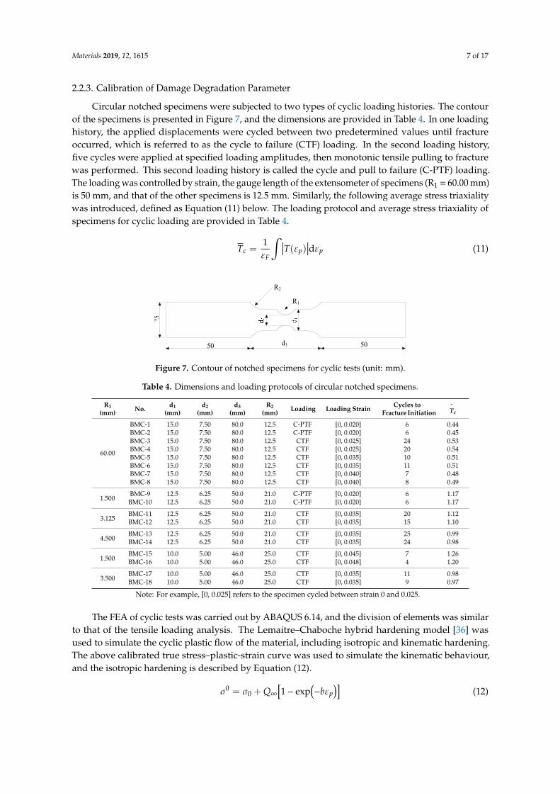
Circular notched specimens were subjected to two types of cyclic loading histories. The contourof the specimens is presented in Figure 7, and the dimensions are provided in Table 4. In one loadinghistory, the applied displacements were cycled between two predetermined values until fractureoccurred, which is referred to as the cycle to failure (CTF) loading. In the second loading history,five cycles were applied at specified loading amplitudes, then monotonic tensile pulling to fracturewas performed. This second loading history is called the cycle and pull to failure (C-PTF) loading.The loading was controlled by strain, the gauge length of the extensometer of specimens (R1 = 60.00 mm)is 50 mm, and that of the other specimens is 12.5 mm. Similarly, the following average stress triaxialitywas introduced, defined as Equation (11) below. The loading protocol and average stress triaxiality ofspecimens for cyclic loading are provided in Table 4.

Tc =1εF

∫ ∣∣∣T(εp)∣∣∣dεp (11)

Materials 2019, 12, x FOR PEER REVIEW 7 of 17

3.75 BM-3 1.64 0.89 1.92 BM-4 1.80 0.92 2.10

7.50 BM-5 3.18 0.69 2.30 BM-6 3.00 0.68 2.15

30.0 BM-7 4.35 0.54 1.98 BM-8 4.36 0.54 1.99

60.0 BM-9 5.05 0.49 1.78 BM-10 5.32 0.50 1.98

Mean value 2.03 Cov/% 6.56

2.2.3. Calibration of Damage Degradation Parameter

Circular notched specimens were subjected to two types of cyclic loading histories. The contour of the specimens is presented in Figure 7, and the dimensions are provided in Table 4. In one loading history, the applied displacements were cycled between two predetermined values until fracture occurred, which is referred to as the cycle to failure (CTF) loading. In the second loading history, five cycles were applied at specified loading amplitudes, then monotonic tensile pulling to fracture was performed. This second loading history is called the cycle and pull to failure (C-PTF) loading. The loading was controlled by strain, the gauge length of the extensometer of specimens (R1 = 60.00 mm) is 50 mm, and that of the other specimens is 12.5 mm. Similarly, the following average stress triaxiality was introduced, defined as Equation (11) below. The loading protocol and average stress triaxiality of specimens for cyclic loading are provided in Table 4.

1 ( )dc p pF

T T ε εε

= (11)

Figure 7. Contour of notched specimens for cyclic tests (unit: mm).

Table 4. Dimensions and loading protocols of circular notched specimens.

R1(mm) No. d1(mm) d2(mm) d3(mm) R2(mm) Loading Loading Strain

Cycles to Fracture

Initiation cT

60.00

BMC-1 15.0 7.50 80.0 12.5 C-PTF [0, 0.020] 6 0.44 BMC-2 15.0 7.50 80.0 12.5 C-PTF [0, 0.020] 6 0.45 BMC-3 15.0 7.50 80.0 12.5 CTF [0, 0.025] 24 0.53 BMC-4 15.0 7.50 80.0 12.5 CTF [0, 0.025] 20 0.54 BMC-5 15.0 7.50 80.0 12.5 CTF [0, 0.035] 10 0.51 BMC-6 15.0 7.50 80.0 12.5 CTF [0, 0.035] 11 0.51 BMC-7 15.0 7.50 80.0 12.5 CTF [0, 0.040] 7 0.48 BMC-8 15.0 7.50 80.0 12.5 CTF [0, 0.040] 8 0.49

1.500 BMC-9 12.5 6.25 50.0 21.0 C-PTF [0, 0.020] 6 1.17 BMC-

10 12.5 6.25 50.0 21.0 C-PTF [0, 0.020] 6 1.17

3.125

BMC-11

12.5 6.25 50.0 21.0 CTF [0, 0.035] 20 1.12

BMC-12

12.5 6.25 50.0 21.0 CTF [0, 0.035] 15 1.10

R1

d350 50

R2

Figure 7. Contour of notched specimens for cyclic tests (unit: mm).

Table 4. Dimensions and loading protocols of circular notched specimens.

R1(mm) No. d1

(mm)d2

(mm)d3

(mm)R2

(mm) Loading Loading Strain Cycles toFracture Initiation

¯Tc

60.00

BMC-1 15.0 7.50 80.0 12.5 C-PTF [0, 0.020] 6 0.44BMC-2 15.0 7.50 80.0 12.5 C-PTF [0, 0.020] 6 0.45BMC-3 15.0 7.50 80.0 12.5 CTF [0, 0.025] 24 0.53BMC-4 15.0 7.50 80.0 12.5 CTF [0, 0.025] 20 0.54BMC-5 15.0 7.50 80.0 12.5 CTF [0, 0.035] 10 0.51BMC-6 15.0 7.50 80.0 12.5 CTF [0, 0.035] 11 0.51BMC-7 15.0 7.50 80.0 12.5 CTF [0, 0.040] 7 0.48BMC-8 15.0 7.50 80.0 12.5 CTF [0, 0.040] 8 0.49

1.500BMC-9 12.5 6.25 50.0 21.0 C-PTF [0, 0.020] 6 1.17BMC-10 12.5 6.25 50.0 21.0 C-PTF [0, 0.020] 6 1.17

3.125BMC-11 12.5 6.25 50.0 21.0 CTF [0, 0.035] 20 1.12BMC-12 12.5 6.25 50.0 21.0 CTF [0, 0.035] 15 1.10

4.500BMC-13 12.5 6.25 50.0 21.0 CTF [0, 0.035] 25 0.99BMC-14 12.5 6.25 50.0 21.0 CTF [0, 0.035] 24 0.98

1.500BMC-15 10.0 5.00 46.0 25.0 CTF [0, 0.045] 7 1.26BMC-16 10.0 5.00 46.0 25.0 CTF [0, 0.048] 4 1.20

3.500BMC-17 10.0 5.00 46.0 25.0 CTF [0, 0.035] 11 0.98BMC-18 10.0 5.00 46.0 25.0 CTF [0, 0.035] 9 0.97

Note: For example, [0, 0.025] refers to the specimen cycled between strain 0 and 0.025.

The FEA of cyclic tests was carried out by ABAQUS 6.14, and the division of elements was similarto that of the tensile loading analysis. The Lemaitre–Chaboche hybrid hardening model [36] wasused to simulate the cyclic plastic flow of the material, including isotropic and kinematic hardening.The above calibrated true stress–plastic-strain curve was used to simulate the kinematic behaviour,and the isotropic hardening is described by Equation (12).

σ0 = σ0 + Q∞[1− exp

(−bεp

)](12)

Materials 2019, 12, 1615 8 of 17

where σ0 represents the size of the initial yielding surface;Q∞ indicates the maximum change value ofyielding surface; and b denotes the changing rate of yielding surface size as plastic strain develops.The parameters Q∞ and b were determined from a trial procedure based on the best fit between thetest curves and FEA curves.

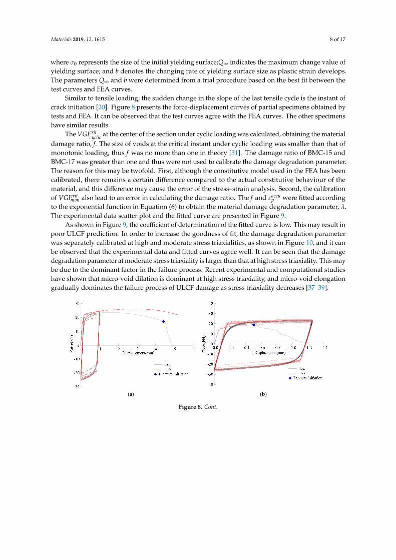
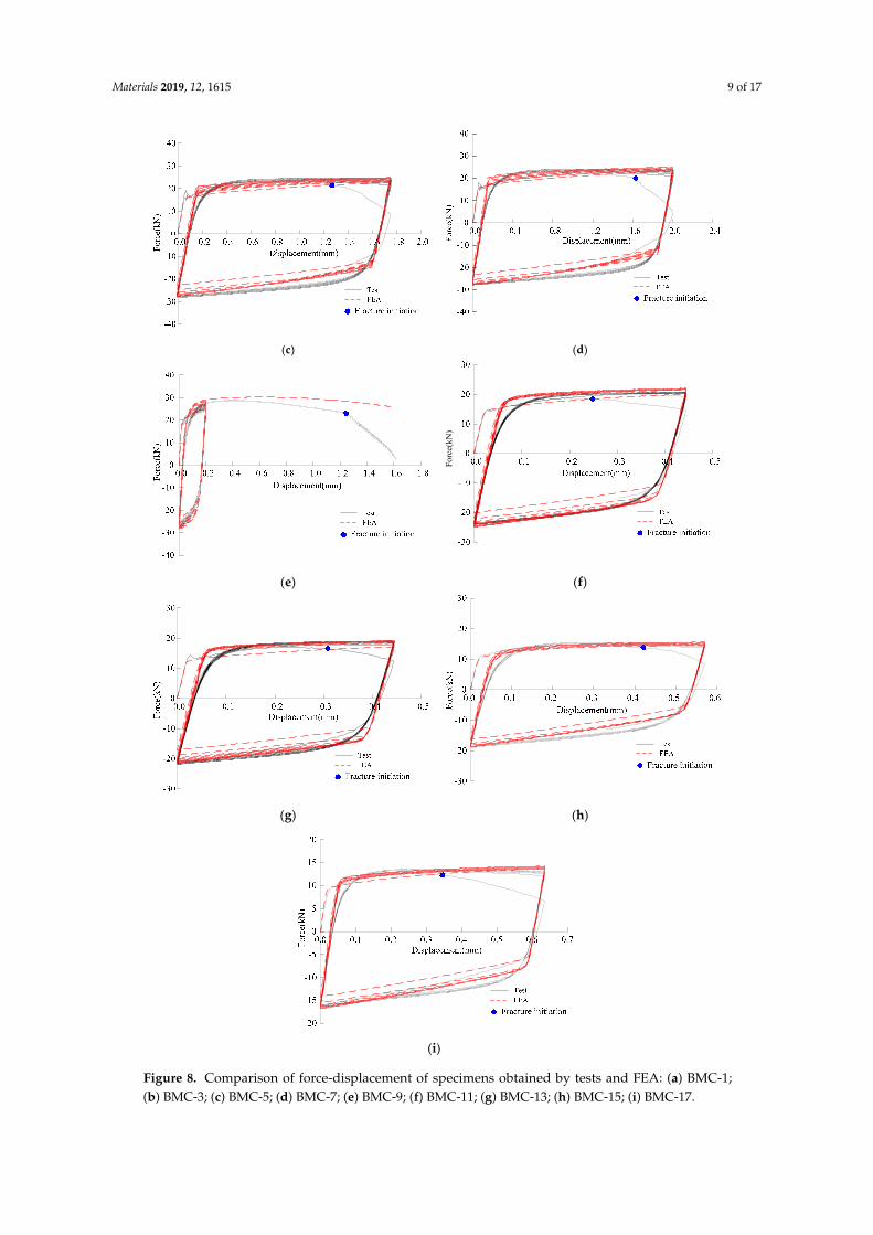
Similar to tensile loading, the sudden change in the slope of the last tensile cycle is the instant ofcrack initiation [20]. Figure 8 presents the force-displacement curves of partial specimens obtained bytests and FEA. It can be observed that the test curves agree with the FEA curves. The other specimenshave similar results.

The VGIcritcyclic at the center of the section under cyclic loading was calculated, obtaining the material

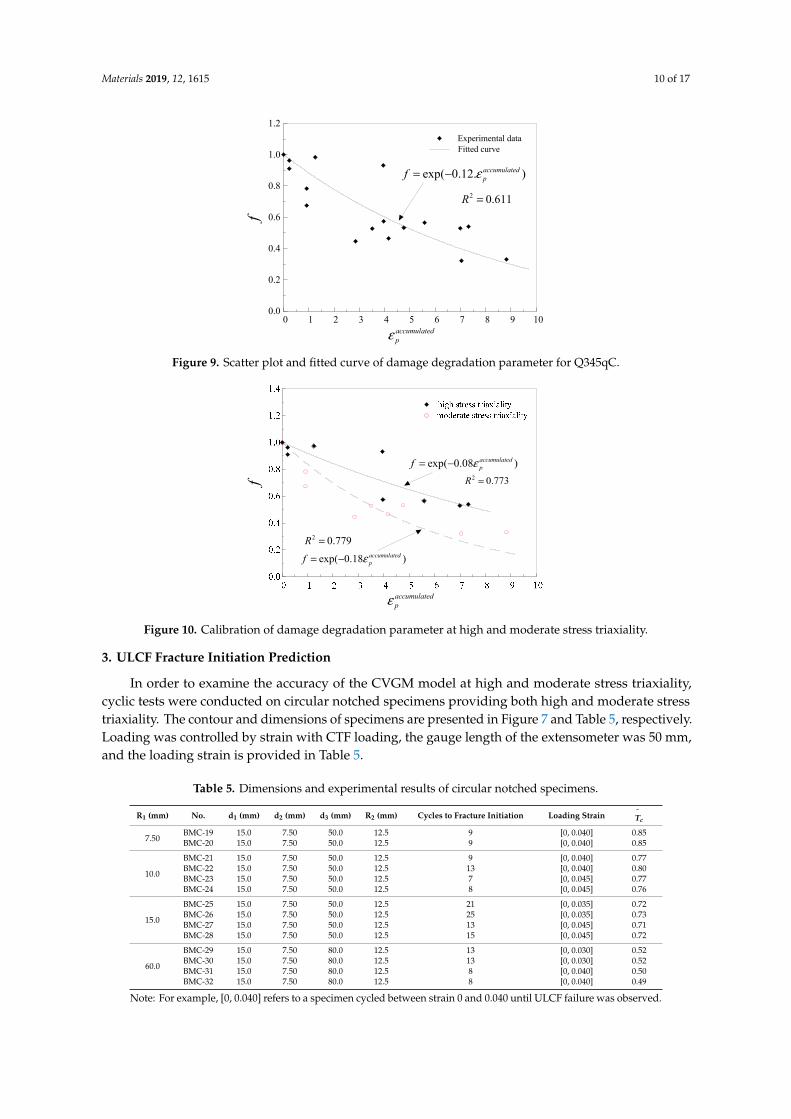
damage ratio, f. The size of voids at the critical instant under cyclic loading was smaller than that ofmonotonic loading, thus f was no more than one in theory [31]. The damage ratio of BMC-15 andBMC-17 was greater than one and thus were not used to calibrate the damage degradation parameter.The reason for this may be twofold. First, although the constitutive model used in the FEA has beencalibrated, there remains a certain difference compared to the actual constitutive behaviour of thematerial, and this difference may cause the error of the stress–strain analysis. Second, the calibrationof VGIcrit

mon also lead to an error in calculating the damage ratio. The f and εaccup were fitted according

to the exponential function in Equation (6) to obtain the material damage degradation parameter, λ.The experimental data scatter plot and the fitted curve are presented in Figure 9.

As shown in Figure 9, the coefficient of determination of the fitted curve is low. This may result inpoor ULCF prediction. In order to increase the goodness of fit, the damage degradation parameterwas separately calibrated at high and moderate stress triaxialities, as shown in Figure 10, and it canbe observed that the experimental data and fitted curves agree well. It can be seen that the damagedegradation parameter at moderate stress triaxiality is larger than that at high stress triaxiality. This maybe due to the dominant factor in the failure process. Recent experimental and computational studieshave shown that micro-void dilation is dominant at high stress triaxiality, and micro-void elongationgradually dominates the failure process of ULCF damage as stress triaxiality decreases [37–39].

Materials 2019, 12, x FOR PEER REVIEW 8 of 17

4.500

BMC-13

12.5 6.25 50.0 21.0 CTF [0, 0.035] 25 0.99

BMC-14

12.5 6.25 50.0 21.0 CTF [0, 0.035] 24 0.98

1.500

BMC-15

10.0 5.00 46.0 25.0 CTF [0, 0.045] 7 1.26

BMC-16

10.0 5.00 46.0 25.0 CTF [0, 0.048] 4 1.20

3.500

BMC-17

10.0 5.00 46.0 25.0 CTF [0, 0.035] 11 0.98

BMC-18

10.0 5.00 46.0 25.0 CTF [0, 0.035] 9 0.97

Note: For example, [0, 0.025] refers to the specimen cycled between strain 0 and 0.025.

The FEA of cyclic tests was carried out by ABAQUS 6.14, and the division of elements was similar to that of the tensile loading analysis. The Lemaitre–Chaboche hybrid hardening model [36] was used to simulate the cyclic plastic flow of the material, including isotropic and kinematic hardening. The above calibrated true stress–plastic-strain curve was used to simulate the kinematic behaviour, and the isotropic hardening is described by Equation (12).

( )00 1 exp pQ bσ σ ε∞ = + − − (12)

where 0σ represents the size of the initial yielding surface;Q∞ indicates the maximum change value of yielding surface; and b denotes the changing rate of yielding surface size as plastic strain develops.

The parameters Q∞ and b were determined from a trial procedure based on the best fit between the test curves and FEA curves.

Similar to tensile loading, the sudden change in the slope of the last tensile cycle is the instant of crack initiation [20]. Figure 8 presents the force-displacement curves of partial specimens obtained by tests and FEA. It can be observed that the test curves agree with the FEA curves. The other specimens have similar results.

(a) (b)

Figure 8. Cont.

Materials 2019, 12, 1615 9 of 17Materials 2019, 12, x FOR PEER REVIEW 9 of 17

(c) (d)

(e) (f)

(g) (h)

(i)

Forc

e(kN

)

Figure 8. Comparison of force-displacement of specimens obtained by tests and FEA: (a) BMC-1;(b) BMC-3; (c) BMC-5; (d) BMC-7; (e) BMC-9; (f) BMC-11; (g) BMC-13; (h) BMC-15; (i) BMC-17.

Materials 2019, 12, 1615 10 of 17

Materials 2019, 12, x FOR PEER REVIEW 10 of 17

(i) Figure 8. Comparison of force-displacement of specimens obtained by tests and FEA: (a) BMC-1; (b) BMC-3; (c) BMC-5; (d) BMC-7; (e) BMC-9; (f) BMC-11; (g) BMC-13; (h) BMC-15; (i) BMC-17.

The critcyclicVGI

at the center of the section under cyclic loading was calculated, obtaining the material damage ratio, f. The size of voids at the critical instant under cyclic loading was smaller than that of monotonic loading, thus f was no more than one in theory [31]. The damage ratio of BMC-15 and BMC-17 was greater than one and thus were not used to calibrate the damage degradation parameter. The reason for this may be twofold. First, although the constitutive model used in the FEA has been calibrated, there remains a certain difference compared to the actual constitutive behaviour of the material, and this difference may cause the error of the stress–strain analysis. Second, the

calibration of critmonVGI also lead to an error in calculating the damage ratio. The f and

accupε

were fitted according to the exponential function in Equation (6) to obtain the material damage degradation parameter, λ. The experimental data scatter plot and the fitted curve are presented in Figure 9.

Figure 9. Scatter plot and fitted curve of damage degradation parameter for Q345qC.

As shown in Figure 9, the coefficient of determination of the fitted curve is low. This may result in poor ULCF prediction. In order to increase the goodness of fit, the damage degradation parameter was separately calibrated at high and moderate stress triaxialities, as shown in Figure 10, and it can be observed that the experimental data and fitted curves agree well. It can be seen that the damage degradation parameter at moderate stress triaxiality is larger than that at high stress triaxiality. This may be due to the dominant factor in the failure process. Recent experimental and computational studies have shown that micro-void dilation is dominant at high stress triaxiality, and micro-void elongation gradually dominates the failure process of ULCF damage as stress triaxiality decreases [37–39].

0 1 2 3 4 5 6 7 8 9 100.0

0.2

0.4

0.6

0.8

1.0

1.2Experimental dataFitted curve

accumulatedpε

f

exp( 0.12. ) accumulatedpf ε= −

2 0.611R =

Figure 9. Scatter plot and fitted curve of damage degradation parameter for Q345qC.Materials 2019, 12, x FOR PEER REVIEW 11 of 17

Figure 10. Calibration of damage degradation parameter at high and moderate stress triaxiality.

3. ULCF Fracture Initiation Prediction

In order to examine the accuracy of the CVGM model at high and moderate stress triaxiality, cyclic tests were conducted on circular notched specimens providing both high and moderate stress triaxiality. The contour and dimensions of specimens are presented in Figure 7 and Table 5, respectively. Loading was controlled by strain with CTF loading, the gauge length of the extensometer was 50 mm, and the loading strain is provided in Table 5.

Table 5. Dimensions and experimental results of circular notched specimens.

R1 (mm) No. d1 (mm) d2 (mm) d3 (mm) R2 (mm) Cycles to Fracture Initiation

Loading Strain cT

7.50 BMC-19 15.0 7.50 50.0 12.5 9 [0, 0.040] 0.85 BMC-20 15.0 7.50 50.0 12.5 9 [0, 0.040] 0.85

10.0

BMC-21 15.0 7.50 50.0 12.5 9 [0, 0.040] 0.77 BMC-22 15.0 7.50 50.0 12.5 13 [0, 0.040] 0.80 BMC-23 15.0 7.50 50.0 12.5 7 [0, 0.045] 0.77 BMC-24 15.0 7.50 50.0 12.5 8 [0, 0.045] 0.76

15.0

BMC-25 15.0 7.50 50.0 12.5 21 [0, 0.035] 0.72 BMC-26 15.0 7.50 50.0 12.5 25 [0, 0.035] 0.73 BMC-27 15.0 7.50 50.0 12.5 13 [0, 0.045] 0.71 BMC-28 15.0 7.50 50.0 12.5 15 [0, 0.045] 0.72

60.0

BMC-29 15.0 7.50 80.0 12.5 13 [0, 0.030] 0.52 BMC-30 15.0 7.50 80.0 12.5 13 [0, 0.030] 0.52 BMC-31 15.0 7.50 80.0 12.5 8 [0, 0.040] 0.50 BMC-32 15.0 7.50 80.0 12.5 8 [0, 0.040] 0.49

Note: For example, [0, 0.040] refers to a specimen cycled between strain 0 and 0.040 until ULCF failure was observed.

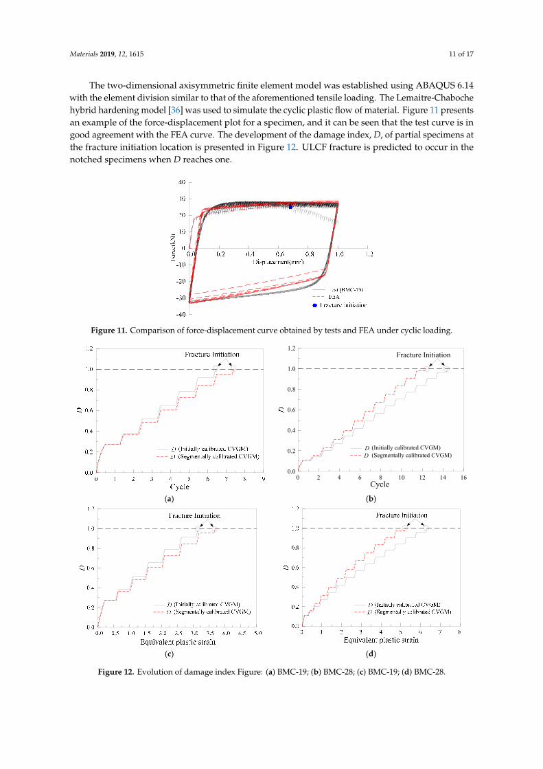
The two-dimensional axisymmetric finite element model was established using ABAQUS 6.14 with the element division similar to that of the aforementioned tensile loading. The Lemaitre-Chaboche hybrid hardening model [36] was used to simulate the cyclic plastic flow of material. Figure 11 presents an example of the force-displacement plot for a specimen, and it can be seen that the test curve is in good agreement with the FEA curve. The development of the damage index, D, of partial specimens at the fracture initiation location is presented in Figure 12. ULCF fracture is predicted to occur in the notched specimens when D reaches one.

accumulatedpε

f

exp( 0.08 )accumulatedpf ε= −

2 0.773R =

exp( 0.18 )accumulatedpf ε= −

2 0.779R =

Figure 10. Calibration of damage degradation parameter at high and moderate stress triaxiality.

3. ULCF Fracture Initiation Prediction

In order to examine the accuracy of the CVGM model at high and moderate stress triaxiality,cyclic tests were conducted on circular notched specimens providing both high and moderate stresstriaxiality. The contour and dimensions of specimens are presented in Figure 7 and Table 5, respectively.Loading was controlled by strain with CTF loading, the gauge length of the extensometer was 50 mm,and the loading strain is provided in Table 5.

Table 5. Dimensions and experimental results of circular notched specimens.

R1 (mm) No. d1 (mm) d2 (mm) d3 (mm) R2 (mm) Cycles to Fracture Initiation Loading Strain ¯Tc

7.50BMC-19 15.0 7.50 50.0 12.5 9 [0, 0.040] 0.85BMC-20 15.0 7.50 50.0 12.5 9 [0, 0.040] 0.85

10.0

BMC-21 15.0 7.50 50.0 12.5 9 [0, 0.040] 0.77BMC-22 15.0 7.50 50.0 12.5 13 [0, 0.040] 0.80BMC-23 15.0 7.50 50.0 12.5 7 [0, 0.045] 0.77BMC-24 15.0 7.50 50.0 12.5 8 [0, 0.045] 0.76

15.0

BMC-25 15.0 7.50 50.0 12.5 21 [0, 0.035] 0.72BMC-26 15.0 7.50 50.0 12.5 25 [0, 0.035] 0.73BMC-27 15.0 7.50 50.0 12.5 13 [0, 0.045] 0.71BMC-28 15.0 7.50 50.0 12.5 15 [0, 0.045] 0.72

60.0

BMC-29 15.0 7.50 80.0 12.5 13 [0, 0.030] 0.52BMC-30 15.0 7.50 80.0 12.5 13 [0, 0.030] 0.52BMC-31 15.0 7.50 80.0 12.5 8 [0, 0.040] 0.50BMC-32 15.0 7.50 80.0 12.5 8 [0, 0.040] 0.49

Note: For example, [0, 0.040] refers to a specimen cycled between strain 0 and 0.040 until ULCF failure was observed.

Materials 2019, 12, 1615 11 of 17

The two-dimensional axisymmetric finite element model was established using ABAQUS 6.14with the element division similar to that of the aforementioned tensile loading. The Lemaitre-Chabochehybrid hardening model [36] was used to simulate the cyclic plastic flow of material. Figure 11 presentsan example of the force-displacement plot for a specimen, and it can be seen that the test curve is ingood agreement with the FEA curve. The development of the damage index, D, of partial specimens atthe fracture initiation location is presented in Figure 12. ULCF fracture is predicted to occur in thenotched specimens when D reaches one.Materials 2019, 12, x FOR PEER REVIEW 12 of 17

Figure 11. Comparison of force-displacement curve obtained by tests and FEA under cyclic loading.

(a) (b)

(c) (d)

Figure 12. Evolution of damage index Figure: (a) BMC-19; (b) BMC-28; (c) BMC-19; (d) BMC-28.

Figure 13 presents the comparison of the experimental results and predicted results, including

the number of cycles, Nf , and equivalent plastic strain, pε, to fracture initiation. To evaluate the

prediction accuracy of the CVGM model, relative error,γ , is calculated according to Equation (13), and the results are presented in Table 6. The results indicate that the predicted life and equivalent plastic strain by a segmentally calibrated CVGM model is nearer to the experimental results compared to the originally calibrated CVGM model. For a small part of specimens, the errors are larger than or close to 25% between experimental results and predicted results by segmentally calibrated CVGM model, which may be related to some assumptions introduced in the model, but the error is acceptable. In general, the mean value of γ calculated by the segmentally calibrated

0 2 4 6 8 10 12 14 160.0

0.2

0.4

0.6

0.8

1.0

1.2Fracture Initiation

Cycle

DD (Segmentally calibrated CVGM)

(Initially calibrated CVGM)

Figure 11. Comparison of force-displacement curve obtained by tests and FEA under cyclic loading.

Materials 2019, 12, x FOR PEER REVIEW 12 of 17

Figure 11. Comparison of force-displacement curve obtained by tests and FEA under cyclic loading.

(a) (b)

(c) (d)

Figure 12. Evolution of damage index Figure: (a) BMC-19; (b) BMC-28; (c) BMC-19; (d) BMC-28.

Figure 13 presents the comparison of the experimental results and predicted results, including

the number of cycles, Nf , and equivalent plastic strain, pε, to fracture initiation. To evaluate the

prediction accuracy of the CVGM model, relative error,γ , is calculated according to Equation (13), and the results are presented in Table 6. The results indicate that the predicted life and equivalent plastic strain by a segmentally calibrated CVGM model is nearer to the experimental results compared to the originally calibrated CVGM model. For a small part of specimens, the errors are larger than or close to 25% between experimental results and predicted results by segmentally calibrated CVGM model, which may be related to some assumptions introduced in the model, but the error is acceptable. In general, the mean value of γ calculated by the segmentally calibrated

0 2 4 6 8 10 12 14 160.0

0.2

0.4

0.6

0.8

1.0

1.2Fracture Initiation

Cycle

DD (Segmentally calibrated CVGM)

(Initially calibrated CVGM)

Figure 12. Evolution of damage index Figure: (a) BMC-19; (b) BMC-28; (c) BMC-19; (d) BMC-28.

Materials 2019, 12, 1615 12 of 17

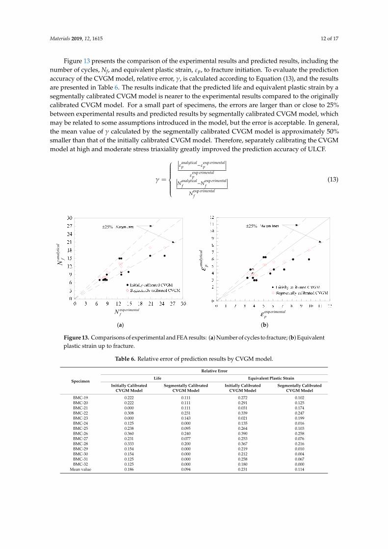
Figure 13 presents the comparison of the experimental results and predicted results, including thenumber of cycles, Nf, and equivalent plastic strain, εp, to fracture initiation. To evaluate the predictionaccuracy of the CVGM model, relative error, γ, is calculated according to Equation (13), and the resultsare presented in Table 6. The results indicate that the predicted life and equivalent plastic strain by asegmentally calibrated CVGM model is nearer to the experimental results compared to the originallycalibrated CVGM model. For a small part of specimens, the errors are larger than or close to 25%between experimental results and predicted results by segmentally calibrated CVGM model, whichmay be related to some assumptions introduced in the model, but the error is acceptable. In general,the mean value of γ calculated by the segmentally calibrated CVGM model is approximately 50%smaller than that of the initially calibrated CVGM model. Therefore, separately calibrating the CVGMmodel at high and moderate stress triaxiality greatly improved the prediction accuracy of ULCF.

γ =

∣∣∣∣εanalytical

p −εexp erimentalp

∣∣∣∣ε

exp erimentalp∣∣∣∣Nanalytical

f −Nexp erimentalf

∣∣∣∣Nexp erimental

f

(13)

Materials 2019, 12, x FOR PEER REVIEW 13 of 17

CVGM model is approximately 50% smaller than that of the initially calibrated CVGM model. Therefore, separately calibrating the CVGM model at high and moderate stress triaxiality greatly improved the prediction accuracy of ULCF.

exp

exp

exp

exp

analytical erimentalp p

erimentalp

analytical erimentalf f

erimentalf

N NN

ε εε

γ

−

= −

(13)

(a) (b)

Figure 13. Comparisons of experimental and FEA results: (a) Number of cycles to fracture; (b) Equivalent plastic strain up to fracture.

Table 6. Relative error of prediction results by CVGM model.

Specimen

Relative Error Life Equivalent Plastic Strain

Initially Calibrated CVGM Model

Segmentally Calibrated CVGM

Model

Initially Calibrated CVGM

Model

Segmentally Calibrated CVGM

Model BMC-19 0.222 0.111 0.272 0.102 BMC-20 0.222 0.111 0.291 0.125 BMC-21 0.000 0.111 0.031 0.174 BMC-22 0.308 0.231 0.339 0.247 BMC-23 0.000 0.143 0.021 0.199 BMC-24 0.125 0.000 0.135 0.016 BMC-25 0.238 0.095 0.264 0.103 BMC-26 0.360 0.240 0.390 0.258 BMC-27 0.231 0.077 0.253 0.076 BMC-28 0.333 0.200 0.367 0.216 BMC-29 0.154 0.000 0.219 0.010 BMC-30 0.154 0.000 0.212 0.004 BMC-31 0.125 0.000 0.258 0.067 BMC-32 0.125 0.000 0.180 0.000

Mean value 0.186 0.094 0.231 0.114

4. Effect of Damage Degradation Parameter The different values of the damage degradation parameter for Q345qC steel were obtained at

different stress triaxiality ranges. To investigate the effect of the damage degradation parameter on predicting ULCF fracture initiation of steel structural members, the single-column steel bridge pier was applied as the research object. In this study, two fillet welds were used with groove angles of 45° and 56°, as presented in Figure 14. In Figure 14, h represents the height of the pier, B represents the

experimentalfN

analytical

fN

25%± 25%±

analytical

pε

experimentalpε

Figure 13. Comparisons of experimental and FEA results: (a) Number of cycles to fracture; (b) Equivalentplastic strain up to fracture.

Table 6. Relative error of prediction results by CVGM model.

Specimen

Relative Error

Life Equivalent Plastic Strain

Initially CalibratedCVGM Model

Segmentally CalibratedCVGM Model

Initially CalibratedCVGM Model

Segmentally CalibratedCVGM Model

BMC-19 0.222 0.111 0.272 0.102BMC-20 0.222 0.111 0.291 0.125BMC-21 0.000 0.111 0.031 0.174BMC-22 0.308 0.231 0.339 0.247BMC-23 0.000 0.143 0.021 0.199BMC-24 0.125 0.000 0.135 0.016BMC-25 0.238 0.095 0.264 0.103BMC-26 0.360 0.240 0.390 0.258BMC-27 0.231 0.077 0.253 0.076BMC-28 0.333 0.200 0.367 0.216BMC-29 0.154 0.000 0.219 0.010BMC-30 0.154 0.000 0.212 0.004BMC-31 0.125 0.000 0.258 0.067BMC-32 0.125 0.000 0.180 0.000

Mean value 0.186 0.094 0.231 0.114

Materials 2019, 12, 1615 13 of 17

4. Effect of Damage Degradation Parameter

The different values of the damage degradation parameter for Q345qC steel were obtained atdifferent stress triaxiality ranges. To investigate the effect of the damage degradation parameter onpredicting ULCF fracture initiation of steel structural members, the single-column steel bridge pierwas applied as the research object. In this study, two fillet welds were used with groove angles of 45◦

and 56◦, as presented in Figure 14. In Figure 14, h represents the height of the pier, B represents thewidth of the flange, W represents the width of the web, t represents the thickness of the flange and theweb, bs represents the width of the stiffener, ts represents the thickness of the stiffener, td representsthe thickness of the diaphragm and baseplate, and a represents the spacing of the diaphragms. Thegeometric dimensions of the steel bridge pier are listed in Table 7. The axial pressure, P, and horizontalforced displacement, δ, were applied at the top of the pier, and the axial compression ratio is 0.15.The loading pattern is shown in Figure 15, where δy is the horizontal yield displacement of the pier.

Materials 2019, 12, x FOR PEER REVIEW 14 of 17

width of the flange, W represents the width of the web, t represents the thickness of the flange and the web, bs represents the width of the stiffener, ts represents the thickness of the stiffener, td represents the thickness of the diaphragm and baseplate, and a represents the spacing of the diaphragms. The geometric dimensions of the steel bridge pier are listed in Table 7. The axial pressure, P, and horizontal forced displacement, δ, were applied at the top of the pier, and the axial compression ratio is 0.15. The loading pattern is shown in Figure 15, where δy is the horizontal yield displacement of the pier.

Table 7. Geometric dimensions of steel bridge piers.

h/mm B/mm W/mm t/mm a/mm bs/mm ts/mm td/mm 2.5 825 825 20 412 81 10 15

Figure 14. Schematic diagram of single-column steel bridge pier.

Figure 15. Loading pattern.

The numerical analyses were conducted using ABAQUS 6.14. Three-dimensional finite element models of the steel bridge pier were established, as shown in Figure 16. The beam element (B31) was employed to simulate the upper part of the steel bridge pier. The lower part of the pier, Ld, was simulated by the shell element (S4R) where the length of Ld was determined according to the empirical formula for calculating the damaged domain [40]. To obtain the stress–strain history at the bottom of the boundary between the flange and web, the solid element (C3D8R) was used. The MPC-beam connection was adopted between the beam and shell element. The shell and solid element were coupled by Shell-Solid. The most dangerous element in the point of connection between the flange and web was considered to be the calculating element, and the size of the calculating element was 0.20 mm, which is consistent with the characteristic length of Q345qC [34]. The Lemaitre–Chaboche

/y

δδ

Figure 14. Schematic diagram of single-column steel bridge pier.

Table 7. Geometric dimensions of steel bridge piers.

h/mm B/mm W/mm t/mm a/mm bs/mm ts/mm td/mm

2.5 825 825 20 412 81 10 15

Materials 2019, 12, x FOR PEER REVIEW 14 of 17

width of the flange, W represents the width of the web, t represents the thickness of the flange and the web, bs represents the width of the stiffener, ts represents the thickness of the stiffener, td represents the thickness of the diaphragm and baseplate, and a represents the spacing of the diaphragms. The geometric dimensions of the steel bridge pier are listed in Table 7. The axial pressure, P, and horizontal forced displacement, δ, were applied at the top of the pier, and the axial compression ratio is 0.15. The loading pattern is shown in Figure 15, where δy is the horizontal yield displacement of the pier.

Table 7. Geometric dimensions of steel bridge piers.

h/mm B/mm W/mm t/mm a/mm bs/mm ts/mm td/mm 2.5 825 825 20 412 81 10 15

Figure 14. Schematic diagram of single-column steel bridge pier.

Figure 15. Loading pattern.

The numerical analyses were conducted using ABAQUS 6.14. Three-dimensional finite element models of the steel bridge pier were established, as shown in Figure 16. The beam element (B31) was employed to simulate the upper part of the steel bridge pier. The lower part of the pier, Ld, was simulated by the shell element (S4R) where the length of Ld was determined according to the empirical formula for calculating the damaged domain [40]. To obtain the stress–strain history at the bottom of the boundary between the flange and web, the solid element (C3D8R) was used. The MPC-beam connection was adopted between the beam and shell element. The shell and solid element were coupled by Shell-Solid. The most dangerous element in the point of connection between the flange and web was considered to be the calculating element, and the size of the calculating element was 0.20 mm, which is consistent with the characteristic length of Q345qC [34]. The Lemaitre–Chaboche

/y

δδ

Figure 15. Loading pattern.

The numerical analyses were conducted using ABAQUS 6.14. Three-dimensional finite elementmodels of the steel bridge pier were established, as shown in Figure 16. The beam element (B31)was employed to simulate the upper part of the steel bridge pier. The lower part of the pier, Ld,was simulated by the shell element (S4R) where the length of Ld was determined according to the

Materials 2019, 12, 1615 14 of 17

empirical formula for calculating the damaged domain [40]. To obtain the stress–strain history atthe bottom of the boundary between the flange and web, the solid element (C3D8R) was used. TheMPC-beam connection was adopted between the beam and shell element. The shell and solid elementwere coupled by Shell-Solid. The most dangerous element in the point of connection between the flangeand web was considered to be the calculating element, and the size of the calculating element was0.20 mm, which is consistent with the characteristic length of Q345qC [34]. The Lemaitre–Chabochehybrid hardening model was used to simulate the cyclic plastic flow of material, and the modelparameters used are provided in Table 8 [34].

Materials 2019, 12, x FOR PEER REVIEW 15 of 17

hybrid hardening model was used to simulate the cyclic plastic flow of material, and the model parameters used are provided in Table 8 [34].

Table 8. Lemaitre–Chaboche hybrid hardening model parameters of Q345qC steel [34].

Material σ|0 (MPa)

Q∞ (MPa) b C1

(MPa) γ1 C2 (MPa) γ2 C3

(MPa) γ3

Base metal 351.10 13.2 0.60 44373.7 523.8 9346.6 120.2 946.1 18.7 Weld deposit metal 428.45 17.4 0.40 12752.3 160.0 1111.2 160.0 630.5 26.0

Note: The meaning of parameters can be found in the literature [34].

Figure 16. Analytical model of steel bridge piers.

The ULCF life of steel bridge piers with different groove angles was calculated using the above calibrated CVGM model, and the calculation results are shown in Table 9. The predicted ULCF life by segmentally calibrated CVGM model varied by a maximum of 37.5% as compared to the predicted life by initially calibrated CVGM model. Therefore, based on the calculation results, the calibrated damage degradation parameter has a significant influence on the ULCF fracture prediction, and it is important to accurately calibrate the damage degradation parameters under different stress triaxiality ranges. Additionally, due to greater strain concentration, the steel bridge pier with a groove angle of 56° is prone to ULCF damage compared with the steel pier with a groove angle of 45°.

Table 9. Calculation results of ULCF life of steel bridge piers.

Groove Angle Predicted Cycles to ULCF Fracture Initiation

1 2

1

f f

f

N NN−

cT Nf1 Nf2

45° 45 29 35.5% 0.68 56° 8 11 37.5% 0.94

Note: Nf1 indicates the cycles to ULCF by initially calibrated CVGM model; Nf2 indicates the cycles to ULCF by segmentally calibrated CVGM model.

5. Conclusions

In the research presented in this paper, Q345qC steel was selected for study as it is commonly used in the construction of steel bridges in China. A model parameter calibration method that separately calibrates the damage degradation parameter at high and moderate stress triaxiality was proposed. The validity of the CVGM model calibrated by the proposed method was verified based on the tests and FEA. The effect of the damage degradation parameter on predicting the ULCF fracture initiation of steel bridge piers was investigated. Based on the conducted studies, the following conclusions can be drawn:

(1) The goodness of fit is improved when the damage degradation parameter is calibrated separately at high and moderate stress triaxiality. It is shown that the predicted number of cycles

Figure 16. Analytical model of steel bridge piers.

Table 8. Lemaitre–Chaboche hybrid hardening model parameters of Q345qC steel [34].

Material σ|0 (MPa) Q∞ (MPa) b C1 (MPa) γ1 C2 (MPa) γ2 C3 (MPa) γ3

Base metal 351.10 13.2 0.60 44373.7 523.8 9346.6 120.2 946.1 18.7Weld deposit metal 428.45 17.4 0.40 12752.3 160.0 1111.2 160.0 630.5 26.0

Note: The meaning of parameters can be found in the literature [34].

The ULCF life of steel bridge piers with different groove angles was calculated using the abovecalibrated CVGM model, and the calculation results are shown in Table 9. The predicted ULCF life bysegmentally calibrated CVGM model varied by a maximum of 37.5% as compared to the predicted lifeby initially calibrated CVGM model. Therefore, based on the calculation results, the calibrated damagedegradation parameter has a significant influence on the ULCF fracture prediction, and it is importantto accurately calibrate the damage degradation parameters under different stress triaxiality ranges.Additionally, due to greater strain concentration, the steel bridge pier with a groove angle of 56◦ isprone to ULCF damage compared with the steel pier with a groove angle of 45◦.

Table 9. Calculation results of ULCF life of steel bridge piers.

Groove AnglePredicted Cycles to ULCF Fracture Initiation |Nf1−Nf2|

Nf1

¯TcNf1 Nf2

45◦ 45 29 35.5% 0.6856◦ 8 11 37.5% 0.94

Note: Nf1 indicates the cycles to ULCF by initially calibrated CVGM model; Nf2 indicates the cycles to ULCF bysegmentally calibrated CVGM model.

5. Conclusions

In the research presented in this paper, Q345qC steel was selected for study as it is commonly usedin the construction of steel bridges in China. A model parameter calibration method that separatelycalibrates the damage degradation parameter at high and moderate stress triaxiality was proposed.The validity of the CVGM model calibrated by the proposed method was verified based on the tests

Materials 2019, 12, 1615 15 of 17

and FEA. The effect of the damage degradation parameter on predicting the ULCF fracture initiationof steel bridge piers was investigated. Based on the conducted studies, the following conclusions canbe drawn:

(1) The goodness of fit is improved when the damage degradation parameter is calibrated separatelyat high and moderate stress triaxiality. It is shown that the predicted number of cycles andequivalent plastic strain to fracture by the segmentally calibrated CVGM model agree well withthe experimental results. The proposed parameter calibration method greatly improved thepredictive accuracy of the CVGM model compared to the previous method.

(2) From the numerical simulation of steel bridge piers, the value of the damage degradationparameter has a relatively significant influence on the predicted cycles to ULCF fracture initiation.Therefore, it is significant to separately calibrate the damage degradation parameters underdifferent stress triaxiality ranges.

(3) The different values of the damage degradation parameter were obtained at high and moderatestress triaxiality, and it was determined that the value of the damage degradation parameterdepends on stress triaxiality. Therefore, it is clear that the relationship between damagedegradation parameter and stress triaxiality deserves further study in the future.

In future work, additional experimental data are needed to determine the relationship betweendamage degradation parameter and stress triaxiality. Additionally, the different values of damagedegradation parameter at different levels of stress triaxiality may be related to the fracture mechanism,and as such it requires further research. In general, the proposed parameter calibration method thatseparately calibrates parameters under different stress triaxiality ranges is promising.

Author Contributions: Conceptualization, S.L. and X.X.; Data curation, Y.L.; Funding acquisition, X.X.;Investigation, S.L., X.X. and Y.L.; Methodology, S.L. and X.X.; Software, Y.L.; Supervision, X.X.; Validation,X.X.; Writing: original draft, S.L.; Writing: review & editing, S.L.

Funding: This research was funded by Natural Science Foundation of China (No. 51878606).

Acknowledgments: The authors would like to thank the Linjun Xie and Xiaojing Cai for their experimentalsupport and papergoing for checking the spelling of the manuscript.

Conflicts of Interest: The authors declare no conflict of interest. The funders had no role in the design of the study.

References

1. Miller, D.K. Lessons learned from the Northridge earthquake. Eng. Struct. 1998, 20, 249–260. [CrossRef]2. Nakashima, M.; Inoue, K.; Tada, M. Classification of damage to steel buildings observed in the 1995

Hyogoken-Nanbu earthquake. Eng. Struct. 1998, 20, 271–281. [CrossRef]3. Subcommittee on Investigation of Seismic Damage of Steel Structure. Investigation of causes of damage to

steel structure on Hanshin-Awaji earthquake disaster. Proc. JSCE 2000, 64, 17–30. (In Japanese)4. Kuwamura, H.; Yamamoto, K. Ductile Crack as Trigger of Brittle Fracture in Steel. J. Struct. Eng. 1997, 123,

729–735. [CrossRef]5. Tateishi, K.; Chen, T.; Hanji, T. Extremely low cycle fatigue assessment method for un-stiffened cantilever

steel columns. Doboku Gakkai Ronbunshuu A 2008, 64, 288–296. [CrossRef]6. Ge, H.; Kang, L.; Tsumura, Y. Extremely Low-Cycle Fatigue Tests of Thick-Walled Steel Bridge Piers.

J. Bridg. Eng. 2013, 18, 858–870. [CrossRef]7. Ge, H.B.; Ohashi, M.; Tajima, R. Experimental study on ductile crack initiation and its propagation in steel

bridge piers of thick-walled box sections. J. Struct. Eng. JSCE 2007, 53, 493–502. (In Japanese)8. Coffin, L.F.J. A study of the effects of cyclic thermal stresses on a ductile metal. Trans. ASME 1954, 76,

931–950.9. Manson, S.S. Behavior of Materials under Conditions of Thermal Stress; National Advisory Commission on

Aeronautics Report 1170; Lewis Flight Propulsion Laboratory: Cleveland, OH, USA, 1954.10. Ge, H.; Kang, L. A Damage Index-Based Evaluation Method for Predicting the Ductile Crack Initiation in

Steel Structures. J. Earthq. Eng. 2012, 16, 623–643. [CrossRef]

Materials 2019, 12, 1615 16 of 17

11. Ge, H.B.; Luo, X.Q. A seismic performance evaluation method for steel structures against local buckling andextra-low cycle fatigue. J. Earthq. Tsunami 2011, 5, 83–99. [CrossRef]

12. Kang, L.; Ge, H.B. Predicting ductile crack initiation of steel bridge structures due to extremely low-cyclefatigue using local and non-local models. J Earthq Tsunami 2013, 17, 323–349. [CrossRef]

13. Miner, M.A. Cumulative damage in fatigue. J. Appl. Mech. 1945, 67, 159–164.14. Tateishi, K.; Hanji, T.; Minami, K. A prediction model for extremely low cycle fatigue strength of structural

steel. Int. J. Fatigue 2007, 29, 887–896. [CrossRef]15. Xue, L. A unified expression for low cycle fatigue and extremely low cycle fatigue and its implication for

monotonic loading. Int. J. Fatigue 2008, 30, 1691–1698. [CrossRef]16. Pereira, J.; De Jesus, A.M.; Xavier, J.; Fernandes, A.; Fernandes, A. Ultra low-cycle fatigue behaviour of a

structural steel. Eng. Struct. 2014, 60, 214–222. [CrossRef]17. Mear, M.; Hutchinson, J. Influence of yield surface curvature on flow localization in dilatant plasticity.

Mech. Mater. 1985, 4, 395–407. [CrossRef]18. Bonora, N. A nonlinear CDM model for ductile failure. Eng. Fract. Mech. 1997, 58, 11–28. [CrossRef]19. Tong, L.; Huang, X.; Zhou, F.; Chen, Y. Experimental and numerical investigations on extremely-low-cycle

fatigue fracture behavior of steel welded joints. J. Constr. Steel Res. 2016, 119, 98–112. [CrossRef]20. Kanvinde, A.M.; Deierlein, G.G. Cyclic Void Growth Model to Assess Ductile Fracture Initiation in Structural

Steels due to Ultra Low Cycle Fatigue. J. Eng. Mech. 2007, 133, 701–712. [CrossRef]21. Rice, J.R.; Tracey, D.M. On the ductile enlargement of voids in triaxial stress fields. J. Mech. Phys. Solids 1969,

17, 201–217. [CrossRef]22. Myers, A.T.; Deierlein, G.G.; Kanvinde, A.M. Testing and Probabilistic Simulation of Ductile Fracture Initiation

in Structural Steel Components and Weldments; Blume Center TR 170; Stanford University: Stanford, CA,USA, 2009.

23. Fell, B.V.; Kanvinde, A.M.; Deierlein, G.G. Large-Scale Testing and Simulation of Earthquake-Induced UltraLow Cycle Fatigue in Bracing Members Subjected to Cyclic Inelastic Buckling; Blume Center TR172; StanfordUniversity: Stanford, CA, USA, 2010.

24. Zhou, H.; Wang, Y.; Shi, Y.; Xiong, J.; Yang, L. Extremely low cycle fatigue prediction of steel beam-to-columnconnection by using a micro-mechanics based fracture model. Int. J. Fatigue 2013, 48, 90–100. [CrossRef]

25. Liao, F.F. Study on Micromechanical Fracture Criteria of Structural Steels and Its Applications to DuctileFracture Prediction of Connections. Ph.D. Thesis, Tongji University, Shanghai, China, 2007. (In Chinese).

26. Xing, J.H.; Guo, C.L.; Li, Y.Y.; Chen, A.G. Damage coefficient identification of micromechanical fractureprediction models for steel Q235B. J. Harbin Inst. Technol. 2017, 49, 184–188. (In Chinese)

27. Pereira, J.; De Jesus, A.M.; Fernandes, A. A new ultra-low cycle fatigue model applied to the X60 piping steel.Int. J. Fatigue 2016, 93, 201–213. [CrossRef]

28. Pereira, J.; Van Wittenberghe, J.; De Jesus, A.; Thibaux, P.; Correia, J.; Fernandes, A. Damage behaviour offull-scale straight pipes under extreme cyclic bending conditions. J. Constr. Steel Res. 2018, 143, 97–109.[CrossRef]

29. Wen, H.J.; Mahmoud, H. New Model for Ductile Fracture of Metal Alloys. II: Reverse Loading. J. Eng. Mech.2016, 142, 08216002. [CrossRef]

30. Kanvinde, A.M.; Deierlein, G.G. The Void Growth Model and the Stress Modified Critical Strain Model toPredict Ductile Fracture in Structural Steels. J. Struct. Eng. 2006, 132, 1907–1918. [CrossRef]

31. Kanvinde, A.M.; Deierlein, G.G. Micromechanical Simulation of Earthquake-Induced Fracture in Steel Structures;Blume Center TR 145; Stanford University: Stanford, CA, USA, 2004.

32. Ramberg, W.; Osgood, W. Description of Stress–Strain Curves by Three Parameters; NACA Techical Note No.902;National advisory committee for aeronautics: Washington, DC, USA, 1943.

33. Bai, Y.; Wierzbicki, T. A new model of metal plasticity and fracture with pressure and Lode dependence.Int. J. Plast. 2008, 24, 1071–1096. [CrossRef]

34. Liao, Y.H. Research on Ultra Low Cycle Fatigue Properties and Fracture Mechanism of Steel Bridge WeldedJoint. Master’s Thesis, Zhejiang University, Hangzhou, China, 2018. (In Chinese).

35. Liao, F.F.; Wang, W.; Chen, Y.Y. Parameter calibrations and application of micromechanical fracture modelsof structural steels. Struct. Eng. Mech. 2012, 42, 153–174. [CrossRef]

36. Lemaitre, J.; Chaboche, J.L. Mechanics of Solid Materials; Cambridge University Press: Cambridge, UK, 1990.

Materials 2019, 12, 1615 17 of 17

37. Barsoum, I.; Faleskog, J. Rupture mechanisms in combined tension and shear—Experiments. Int. J.Solids Struct. 2007, 44, 1768–1786. [CrossRef]

38. Barsoum, I.; Faleskog, J. Rupture mechanisms in combined tension and shear—Micromechanics. Int. J. SolidsStruct. 2007, 44, 5481–5498. [CrossRef]

39. Danas, K.; Castañeda, P.P. Influence of the Lode parameter and the stresstriaxiality on the failure ofelasto-plastic porous materials. Int. J. Solids Struct. 2012, 49, 1325–1342. [CrossRef]

40. Zhuge, H.Q.; Xie, X.; Tang, Z.Z. Study on length of damaged zone of steel piers under bidirectional horizontalearthquake components. China J. Highway Transp. 2019, in press.

© 2019 by the authors. Licensee MDPI, Basel, Switzerland. This article is an open accessarticle distributed under the terms and conditions of the Creative Commons Attribution(CC BY) license (http://creativecommons.org/licenses/by/4.0/).