Importers, Exporters and the Division of the Gains from Trade · importers. Exporters and importers...
46
* † ‡ * † ‡
Transcript of Importers, Exporters and the Division of the Gains from Trade · importers. Exporters and importers...
Importers, Exporters and the Division of the Gains
from Trade∗
Andrew B. Bernard†
Tuck School of Business at Dartmouth, CEPR & NBER
Swati Dhingra‡
LSE, CEP & CEPR
This Version: October, 2016
Abstract
This paper examines the microstructure of import markets and the division of the gainsfrom trade among consumers, importers and exporters. When exporters and importers transactthrough anonymous markets, double marginalization and business stealing among competingimporters lead to lower pro�ts. Trading parties can overcome these ine�ciencies by investingin richer arrangements such as bilateral contracts that eliminate double marginalization andjoint contracts that also internalize business stealing. Introducing the microstructure of importmarkets into a trade model, we show that trade liberalization increases the incentive to engagein joint contracts, thus raising the pro�ts of these exporters and importers at the expense ofconsumer welfare. We examine the implications of the model for prices, quantities and exporter-importer matches in Colombian import markets before and after the US-Colombia free tradeagreement. US exporters that started to enjoy duty-free access were more likely to increasetheir average price, decrease their quantity exported and reduce the number of import partners.These exporters increased their average tari�-inclusive price by as much as 25%, leading to alow average pass-through rate of less than 4% for all imports that received duty-free access intoColombia.
Keywords: Heterogeneous �rms, exporters, importers, pass through, contracts, microstruc-ture, consumer welfare.JEL codes: F10, F12, F14.
∗We are grateful to John Morrow, Emanuel Ornelas, Gianmarco Ottaviano, Chris Snyder, Catherine Thomas,Dan Tre�er, Tony Venables, Alwyn Young and seminar participants at Aarhus, Berkeley-Stanford, Bologna, ERWIT,FGV Sao Paulo, IIFT, KU Milan, Oslo, Oxford, LSE, Paris, Princeton Summer Workshop, PSU, PUC, Salento,SED, Sussex, Toronto, Tuck (Dartmouth), World Bank and UEA for helpful comments. We thank Giovanni Maggiand Dan Tre�er for detailed discussions and Angela Gu and Yan Liang for excellent research assistance. A previousversion of this paper circulated under the title �Contracting and the Divisions of the Gains from Trade�.†100 Tuck Hall, Hanover, NH 03755, USA, tel: +1 603 646 0302, email: andrew.b.bernard (at) tuck.dartmouth.edu‡Houghton Street, London, WC2A 2AE UK; tel: +44(0)20-7955-7804, email: s.dhingra (at) lse.ac.uk

Importers, Exporters and the Division of the Gains from Trade
1 Introduction
Trade liberalization can generate substantial improvements in welfare through increased product
variety, lower prices and the reallocation of resources from less to more e�cient producers. Domestic
consumers gain from easier access to imports, but they rarely have direct access to foreign products.
Trade is typically between �rms who exercise market power in buying and selling foreign products.
This paper examines how the behavior of importers and their relationships with exporters a�ect the
division of the gains from trade. Trading partners make endogenous choices among di�erent types
of contracts, which gives them di�erent degrees of market power in importing. Trade liberalization
a�ects the incentives for di�erent contracts. This leads to a change in the microstructure of import
markets, which provides a qualitatively new channel for the division of the gains from trade. Foreign
exporters and domestic importers potentially gain market power and bene�t at the expense of
domestic consumers.
In line with the concerns of the European Commission and the Federal Trade Commission,
market integration can induce �rms to replace trade barriers with microstructures that limit the
gains from market access to consumers (Ra� and Schmitt 2005). Typically, foreign competition
is associated with lower price-cost margins (Tybout 2003; Levinsohn 1993; Harrison 1994) but a
growing literature documents that the pass-through of border prices into home market prices is low
in macro studies and in detailed micro work.1 In our framework, the low pass-through of trade
cost reductions into import prices is a result of the changes in the contracts between exporters and
importers.
Exporters and importers operate in thin markets, that do not re�ect anonymous transactions.
Anonymous transactions lead to two ine�ciencies in pro�t maximization. First, when exporters and
importers engage through anonymous market-clearing prices, market power of importers leads to
double marginalization and lower pro�ts. Exporters can overcome this ine�ciency by moving away
from unit prices and o�ering bilateral contracts that specify total payments and quantities. Second,
importers in an anonymous market are unable to internalize the business stealing e�ect of their sales
on competing importers that sell varieties of the same foreign product. An exporter can mitigate
this externality by investing in joint contracts with these competing importers. This leads to higher
pro�ts by restricting sales and driving up prices charged to consumers. We embed the microstructure
of richer contracts into a standard trade model. The microstructure channel reinforces the gains
1See for example Engel and Rogers (1996); Burstein et al. (2003); Campa and Goldberg (2005) in the macroliterature. Detailed micro studies include Ganslandt and Maskus (2004) for Swedish pharmaceuticals, De Loeckeret al. (2012) and Mallick and Marques (2008) for Indian manufacturing, Badinger (2007) for manufacturing andservices in the European Single Market, and Konings et al. (2005) for Bulgarian and Romanian manufacturingindustries.
1

Importers, Exporters and the Division of the Gains from Trade
from trade when �rms enter into bilateral contracts that mitigate double marginalization. But as
�rms start to invest in internalizing business stealing, trade liberalization increases their market
power and a�ects the division of the gains from trade. They engage in complex relationships to
overcome the ine�ciencies of anonymous markets.
In our model, market expansion increases the returns to joint contracts, relative to bilateral
contracts. This is because market expansion enables �rms to better amortize the higher �xed costs
of joint contracts and because import competition does less damage to the pro�ts of �rms with
greater market power. As �rms switch to joint contracts, they internalize the business stealing
e�ect of their sales. They raise consumer prices and get more of the surplus from consumers. We
show that the microstructure e�ect is a new channel for the gains from trade that goes beyond the
standard gains from variety expansion and pro-competitive e�ects, and that increases pro�ts at the
expense of consumer welfare.
To test for the microstructure e�ect, we would ideally like to examine the impact of trade
liberalization on the actual relationships between exporters and importers. Such data is unavailable
so we examine the distinct observable implications for prices, quantities and exporter-importer
matches during a period of trade liberalization. If the microstructure matters, trade liberalization
will induce exporters to consolidate their import market. They will bene�t from higher prices by
scaling back on the quantity they sell and the number of importing partners that they sell to in
the liberalizing country. We test these implications for Colombian imports before and after the US-
Colombia Free Trade Agreement (FTA) using transaction-level matched importer-exporter data. In
keeping with the theory, we �nd that US exporters whose products started to enjoy duty-free access
through the FTA were more likely to simultaneously increase their import price, lower their quantity
and reduce the number of their importer partners in Colombia. This con�rms the Metzler paradox
of domestic prices rising in response to tari� reductions and we �nd that it persists after adjusting
for quality in prices. Among exporters with more than $10,000 of sales in the Colombian market,
�rms in the �rst and second terciles of initial size increased their free-on-board import prices by 8
to 30% on average. This contributed to a less than 4% average reduction in tari�-inclusive prices
for all Colombian imports that received duty-free access.
The main theoretical contribution of the paper is to provide a model that embeds two-sided
market power in a general equilibrium setting. We build on the vertical relations literature in
industrial organization to model the relationship between exporters and importers (Hart and Tirole
1990). While a large literature examines these relationships, its focus is on �rm behavior, typically
in a stylized setting of two buyers and sellers. We embed the �rm behavior in a general equilibrium
setting with multiple �rms, which is important for understanding the gains from trade because they
are also a�ected by the labor market and by �rms' decisions to enter and exit product markets.This
is also useful in taking the theoretical predictions to trade data that is usually available through
2

Importers, Exporters and the Division of the Gains from Trade
�rm-level customs transactions.
Our focus on vertical relations is related to work in international trade on intermediation (Ak-
erman 2010; Bernard et al. 2010; Blum et al. 2010; Ahn et al. 2011; Atkin and Donaldson 2012),
retailing (Eckel 2009; Ra� and Schmitt 2012; Blanchard et al. 2013) and vertical integration (Feen-
stra et al. 2003; Antràs and Helpman 2004; Conconi et al. 2012). As is well-known, embedding
two-sided market power in general equilibrium gives intractable models so many of these papers
focus on �rm characteristics and abstract from the market power of importers. Ra� and Schmitt
(2005, 2009) examine importer market power in an oligopoly model of trade and retailing to show
trade liberalization can reduce welfare due to vertical restraints. We embed vertical restraints in a
general setting with many heterogeneous exporters and importers to obtain predictions that can be
taken to the data. We obtain tractability by using the tools developed in the variable markups lit-
erature under monopolistic competition (Parenti et al. (2014); Neary and Mrazova (2013); Dhingra
and Morrow (2012); Mayer et al. (2014)). This enables us to generalize the results for �rm behavior
to a wide class of demand functions, which is important in revealing new gains from trade that do
not arise under the knife-edge cases of standard demand systems.
The focus on consumption side gains is similar to a large literature on the impact of trade
liberalization on markups and prices. Tybout (2003) surveys the research using industry-level data
and plant-level panel data and concludes that most studies �nd higher industry-level exposure
to foreign competition is associated with lower price-cost margins or markups, e.g. Levinsohn
(1993); Harrison et al. (2005). The pass-through of reductions in trade costs to domestic prices is
typically low, and recent studies �nd the behavior of domestic �rms determines the extent to which
trade policy a�ects prices at home. Mallick and Marques (2008) �nd low tari� rate pass-through
into import prices in Indian manufacturing during the liberalization of 1991. De Loecker et al.
(2012) estimate that on average, factory-gate prices fell by 18 percent despite average import tari�
declines of 62 percentage points, as domestic Indian �rms did not pass on the reductions in trade
costs to consumers. Badinger (2007) �nds the European Single Market led to an overall reduction
in markups for manufacturing products, but markups rose in several manufacturing and services
industries that also experienced an increase in industry concentration and average �rm size. In early
work on Japanese imports, Lawrence and Saxonhouse (1991) document that the presence of large
conglomerates at home is associated with lower import penetration, suggesting the import-inhibiting
e�ects of �rms with high market power. Lawrence (1991) argues market power of intermediaries
can explain why Japanese consumer prices were higher than German import prices for the same
export from the US. Yeats (1978) �nds iron and steel prices are higher in more concentrated import
markets. In early theoretical work, Venables (1985) shows unilateral reductions in trade barriers
can increase consumer prices in the liberalizing country when entry and exit induce pro�t shifting
across countries.
3

Importers, Exporters and the Division of the Gains from Trade
Our pricing predictions are consistent with these �ndings, and provide systematic evidence for
the Metzler paradox (Venables 1985; Bagwell and Staiger 2012; Bagwell and Lee 2015). A reduction
in tari�s induces more consolidation in the import market of medium-sized US exporters in Colom-
bia. Previous work has suggested that trade policy is a substitute for competition policy. Small open
economies can increase competition in the domestic market by integrating with world markets and
bene�ting from import competition. Our results show that when exporters and importers operate
in thin markets, trade policy and competition policy are complements. Trade liberalization would
be most bene�cial when competition policy is used in conjunction with trade policy to encourage
�rms to pass on the cost savings to consumers.
We introduce contracting choices to see how market power in import markets changes the gains
from trade. This is related to several di�erent strains of work in international trade. Bernard et al.
(2009), Castellani et al. (2010) and Muuls and Pisu (2009) document substantial heterogeneity across
importing �rms for the US, Italy and Belgium respectively and also show that importers di�er from
non-importers. Papers by Rauch (1999), Rauch and Watson (2004), Antràs and Costinot (2011),
Chaney (2014) and Petropoulou (2011) model the formation of matches between exporters and
importers. These papers adopt a search and matching approach to match formation. Our paper
is also closely related to the recent set of papers using matched exporter-importer data. Blum
et al. (2010, 2012) examine characteristics of trade transactions for the exporter-importer pairs of
Chile-Colombia and Argentina-Chile while Eaton et al. (2014) consider exports of Colombian �rms
to speci�c importing �rms in the United States. Carballo et al. (2013) and Bernard et al. (2014)
use matched data to study the role of buyers in �rm-level trade �ows. We abstract from these
mechanisms and focus on the microstructure of import markets to understand the resulting e�ects
on prices, quantities and the division of the gains from trade. A growing literature also shows how
imported inputs increase the productivity of importers, see Amiti and Konings (2007), Halpern
et al. (2015), Boler et al. (2015) and Fieler et al. (2014). We focus on the consumption side role of
importers.
The rest of the paper is organized as follows: Section 2 introduces a model where exporters
and importers transact through anonymous markets, as a benchmark. We then introduce bilateral
contracts and joint contracts, and show that trade liberalization a�ects the division of the gains
from trade among domestic consumers, home importers, and foreign exporters. Section 3 develops
the testable predictions of the model for prices, quantities, and matches. Section 4 takes the testable
predictions to Colombian import data and Section 5 concludes.
2 Model of Exporters and Importers
This section describes the economy which consists of consumers, exporters and importers. We work
with a standard trade model akin to Krugman (1979), and introduce importers with market power.
4

Importers, Exporters and the Division of the Gains from Trade
As is well-known, two-sided market power in an industry equilibrium often leads to intractable
models. This is why several papers in intermediation abstract from market power at least on one
side of the market. As our focus is on the division of the gains from trade, we model market power of
exporters and importers in an industry equilibrium. We achieve this by using the tools developed in
Dhingra and Morrow (2012) for monopolistic competition trade models. For ease of exposition, we
start with homogeneous �rms in this Section. The next Section examines the testable variety-level
predictions of the theory under �rm heterogeneity and �xed entry.
In a standard setting, exporters sell to importers in anonymous markets which means they set
a unit price at which any importer can buy from them. We �rst model the �rm problem in an
anonymous market with unit prices, and show that market power results in double marginalization
and business stealing among importers of a product. When exporters are not constrained to set unit
prices, exporters and importers choose payments and quantities that maximize their joint pro�ts
by overcoming the externalities induced by an anonymous market. We specify the simplest setting
that departs from anonymous markets to provide a richer microstructure for the import market.
There are two countries, Home and Foreign (with x indexing exports from the foreign country
to the home country). Di�erentiated products are produced at home and abroad, and are further
di�erentiated by domestic �rms (importers) who sell to consumers. The home country has L workers,
each of whom is endowed with a unit of labor and has preferences over consumption goods. We
specify the demand and technology in the next sub-sections, and then discuss �rm decisions under
anonymous markets.
2.1 Preferences
Each worker has identical preferences over varieties of a di�erentiated good. Preferences for di�eren-
tiated goods take the form of nested variable elasticity of substitution (VES) utility. A di�erentiated
product in the upper nest is indexed by i, and is a composite of further di�erentiated variants in
the lower nest which are indexed by ij. The utility function is as follows:
U ≡ˆu(qi)di, qi =
ˆv(qij)dj, u′, v′ > 0, u′′, v′′ < 0.
The VES inverse demand builds on a growing literature of variable markup frameworks like Parenti
et al. (2014); Neary and Mrazova (2013); Dhingra and Morrow (2012); Mayer et al. (2014). The sub-
utility functions u and v are thrice continuously di�erentiable, strictly increasing, strictly concave
on (0,∞), normalized to zero at zero quantities and satisfy Inada conditions. Concavity ensures
that consumers purchase all available varieties and the inverse demand for variety ij is
pij = v′(qij)u′(qj)/δ (1)
5

Importers, Exporters and the Division of the Gains from Trade
where δ is the consumer's budget multiplier. For a worker with income I, the budget multiplier is
δ =
ˆ ˆqijv
′(qij)u′(qj)didj/I.
A well-de�ned equilibrium will require conditions on the demand elasticities across the two nests
of preferences. Following Dhingra and Morrow (2012), the elasticity of utility is εx(q) ≡ x′(q)q/x(q)
for x ∈ {u, v} and the elasticity of marginal utility is µx ≡ −x′′(q)q/x′(q). These elasticities are
bounded below by b > 0 and above by 1− b < 1, and are increasing in q. To �x ideas, CES demand
is x(q) = qρ which implies εx(q) = ρ and µx(q) = 1− ρ are between 0 and 1, and correspond to the
special case with ε′x(q), µ′x(q) = 0. While CES demand provides simple pricing decisions, we depart
from CES demand because it gives knife-edge results that trade liberalization has no impact on the
microstructure, similar to the lack of pro-competitive e�ects in Krugman (1979) and Melitz (2003)
under CES demand.
2.2 Technology
Following Krugman (1980), there are Mc identical producers at home. Each producer supplies a
unique di�erentiated product with a linear technology. Each producer faces a unit cost c. Producers
are monopolistically competitive and pay �xed operation costs fc. Producers cannot directly access
�nal consumers. They must engage distributors to deliver their products to consumers.
There are Md identical distributors at home. Producers at home and abroad must sell through
these distributors to the consumers. Distributors are monopolistically competitive and transform
the producer's product into a di�erentiated variety for �nal consumption. A distributor with unit
cost d transforms producer c's product from x(c) units of production into y(c, d) = x(c)/d units of
the �nal di�erentiated variety. If px(c) is the unit price of variety c charged by the producer, then
the unit cost of a distributor is px(c)d. Under this formulation, distributors perform the function of
lowering the costs of delivery to consumers.
Before proceeding to the equilibrium, we need to specify where the producers and distributors
�t into the nesting structure of demand. To capture rich substitutability patterns, we specify the
upper nest quantity as qj = θqc + (1 − θ)qd for θ ∈ {0, 1}. When θ = 0, qj = qd and distributors
are in the upper nest. For θ = 1, qj = qc and producers are in the upper nest. We will show that
θ = 1 leads to interesting results because the lower nest distributors do not internalize the impact
of their sales on other distributors. This provides a role for richer contracting arrangements and
gives new results for the impact of trade liberalization on the gains from trade. As we will initially
focus on a free trade equilibrium, all �rms will engage in international trade and we will use the
term exporters to denote c �rms and importers to denote d �rms.
6

Importers, Exporters and the Division of the Gains from Trade
2.3 Anonymous Market Equilibrium
A natural way of introducing importers into a standard trade model is through anonymous market
transactions. An exporter chooses the market price for her product and then takes her product to
an import market. The importers choose how much to buy. They further di�erentiate the product
and supply �nal varieties to consumers. Then cd indexes a �nal variety exported by c and imported
by d. We start with this benchmark case of anonymous markets to illustrate the ine�ciencies that
lead to richer relationships between exporters and importers. To formalize the setting, the timing
is as follows.
• Firms pay their �xed costs of operation (fc,fd).
• c chooses her market price px(c).
• d buys xcd units at price px(c).
• Quantities qcd are supplied to �nal consumers at price pcd.
Markets are segmented and we solve for an equilibrium by �rst determining the �nal quantities sold
to consumers. Then we derive the demand for the producer's product and determine the optimal
price chosen by the producer. We abstract from variety-speci�c search costs fcd until the Section
with heterogeneous �rms where they lead to interesting selection e�ects.
2.3.1 Prices in Anonymous Markets
Importer d faces the inverse demand function pcd = v′(qcd)u′ (θqc + (1− θ)qd) /δ. He cannot in-
�uence the aggregate market conditions δ and the producer's total sales in the home country qc.
At unit price pxc of c's product, the importer chooses �nal quantities qcd and his total quantity qd
to maximize pro�ts. His variable pro�t is πd ≡ Mc
(pcd
(qcd, qd, q̂c, δ̂
)− pxcd
)qcdLd where the hat
denotes that the distributor takes these components of the inverse demand as given. Summing the
demand of all importers in the home country xc ≡ MdxcdLd = Mddqcd (pxc )Ld, exporter c chooses
pxc to maximize variable pro�ts πc = Md (pxc − c) dqcd (pxc )Ld.
To ensure a well-de�ned �rm problem, we assume that marginal revenues are decreasing and
that µ′vq < (1− µv) (1− µv − µuεv). We will also assume that µuεv ≤ minµv ·min (1− µv) whichensures that the direct impact of own quantity on price is greater than the indirect impact of other
varieties through the upper nest quantities. This condition is equivalent to the substitutability
restriction of a nested CES demand system and later we will show that it ensures prices are higher
under anonymous markets compared to bilateral and multilateral pro�t maximization among �rms.
Under anonymous markets, the optimal price chosen by d is
pcd = pxcd/
(1− µv(qcd)−
(1− θ)u′(qd)θu′(qc) + (1− θ)u′(qd)
µu(qd)εv(qcd)
)7

Importers, Exporters and the Division of the Gains from Trade
. Using subscripts for brevity, the exporter's optimal price is pxc = c/ (1− γc) where γc ≡ µvcd +
µ′vcdqcd/(
1− µvcd −(1−θ)u′(qd)
θu′(qc)+(1−θ)u′(qd)µu(qd)εvcd
).
Putting the two optimal price functions together, the �nal price of variety cd under anonymous
markets is
pcd = cd/
1− γc︸ ︷︷ ︸Double Marginalization
·
1− µvcd −(1− θ)u′(qd)
θu′(qc)︸ ︷︷ ︸Business Stealing
+(1− θ)u′(qd)µu(qd)εvcd
. (2)
The �rst term in square brackets in Equation 2 is the markup charged by the exporter to the importer
which re�ects the classic double marginalization problem in anonymous markets. Exporters take
into account the derived demand for their product and charge pxc = c/ (1− γc) > c. Importers
further mark up the price (with the term in parenthesis) and consumers end up with having to pay
double markups. This double marginalization leads to lower bilateral pro�ts for c and d due to
reduced sales. If producers and distributors can engage outside of anonymous transactions, then
they need not set market-clearing unit prices. They can specify payments and quantities that get
rid of double marginalization and increase the bilateral pro�ts from their relationship. We will
consider these �bilateral contracts� in the next Section and show that trade liberalization has the
usual e�ect of increasing sales and reducing prices when exporters and importers transact under
bilateral contracts.
The term in parenthesis shows the markup charged by the importer. Importers account for the
cannibalization of their own varieties on each other. This cannibalization translates into higher
�nal markups through µu(qd). But they do not account for the business stealing impact of their
sales on competing distributors of an exporter's product, which can be seen from the denominator
in parenthesis. There is no µu(qc) in the optimal markup and competition among distributors in
the �nal goods market implies that the total pro�t from an exporter's product is not maximized.
We will therefore consider �joint contracts� that maximize the total pro�ts of an exporter and her
importers. While an importer can internalize cannibalization of her own varieties by virtue of being
second in the chain of sales, exporters and importers are unable to overcome the business stealing
externality through anonymous markets.
Anonymous markets therefore provide two reasons for switching to richer contracts. The �rst
reason is that unit pricing in anonymous markets leads to double marginalization which lowers the
bilateral pro�t of an exporter and an importer. Bilaterally pro�t maximizing contracts that specify
payments and quantities can overcome the double marginalization problem and reduce consumer
prices. Importers internalize the cannibalization of their own sales. When importers are in the
upper nest (θ = 0), there is no other reason to enter into richer contracts with the exporters.
Bilateral contracts solve the double marginalization problem and the cannibalization e�ect is already
8

Importers, Exporters and the Division of the Gains from Trade
accounted for. The second reason for �rms to move away from anonymous markets is that importers
do not account for their business stealing e�ects. When exporters are in the upper nest (θ = 1),
there is an incentive for an exporter and her importers to enter into joint contracts to get rid of
business stealing. Consumer prices are higher compared to bilateral contracts because competition
among importers is reduced to maximize multilateral pro�ts of the exporter and her importers.
Bilateral contracts reinforce the usual gains from trade because they reduce consumer prices
further. Joint contracts have the opposite e�ects. Competition in the import market is reduced
to increase the prices faced by consumers. We examine how these richer arrangements between
exporters and importers determine the division of the gains from trade liberalization between ex-
porters, importers and consumers. To avoid a taxonomical analysis, we focus on the case where
exporters are in the upper nest and importers are in the lower nest, so that joint contracts are
desirable. We explain the contracting arrangements that mitigate the externalities of anonymous
markets and proceed to the industry equilibrium under this richer microstructure.
2.4 Microstructure of Import Markets
Exporters and importers often have long-standing and complex relationships. It is therefore likely
that they engage in contracts that overcome the ine�ciencies from anonymous transactions. Fol-
lowing the seminal work of Hart and Tirole (1990), we consider two distinct contracts that overcome
these ine�ciencies. The �rst type of contract overcomes double marginalization by specifying quan-
tities and payments that maximize bilateral pro�ts of the exporter-importer pair. The second type
of contract overcomes double marginalization and business stealing by committing to all quantities
and payments that maximize the joint pro�t of an exporter and her importers.
The main advantage of the Hart-Tirole approach is that we do not need to specify the meth-
ods through which �rms maximize bilateral pro�ts or joint pro�ts, and instead can focus on the
observable outcomes of quantities and payments that result from implementing pro�t-maximizing
contracts. For instance, an exporter can maximize bilateral pro�ts by setting a two-part tari� that
charges the importer a price equal to her marginal cost (px(c) = c), and a �xed fee that recoups
part or all of the bilateral pro�ts without changing sales incentives. The exporter could also have
maximized bilateral pro�ts through resale price maintenance. The importer is then obliged to sell
at a price chosen by the exporter. As we will show later in this Section, when the exporter chooses
the �nal price, the resulting quantity allocation is the same as a two-part tari� and bilateral pro�ts
of the exporter-importer pair are maximized.
The industrial organization literature provides di�erent methods through which �rms avoid
double marginalization and business stealing, such as �xed fees, quantity discounts and resale price
maintenance.2 These are rarely observable, and these methods can often take the form of informal
2This is an area of ongoing research in industrial organization and Miklos-Thal et al. (2010) provide an overview
9

Importers, Exporters and the Division of the Gains from Trade
practices or implicit arrangements that are sustained through repeated interaction. Following Hart
and Tirole (1990), we therefore abstract from the methods used to implement bilateral or joint
pro�t maximization, and focus instead on the implications for observable outcomes, such as quantity
allocations and payments, that are the same across di�erent methods.
We start with bilateral pro�t maximization and then discuss joint pro�t maximization. The
market does not maximize bilateral pro�ts of an exporter-importer pair due to double marginal-
ization. This problem is overcome when an exporter engages in a bilateral private contract with
an importer. The bilateral contract speci�es a �nal quantity and a payment to be made to the
exporter (qcd and Tcd). As the exporter no longer relies on unit prices that are marked up, the
�nal quantity is chosen to maximize the bilateral pro�t of the exporter-importer pair. Following
Horn and Wolinsky (1988), the exporter and the importer split the bilateral pro�ts through Nash
bargaining, and this determines the payments from the importer to the exporter. The bilateral
contract overcomes double marginalization and results in higher quantities and lower prices for the
�nal consumers.
But bilateral contracts do not mitigate the business stealing externality imposed by importers
on each other. The competition between di�erent importers implies that prices are lower than
the monopolistic price that the exporter would have chosen. The key insight of Hart and Tirole
(1990) is that a seller cannot commit to selling lower quantities of her product because she would
prefer to bypass her existing buyers and sell more to earn higher pro�ts. Even though the exporter
could o�er contracts that account for the business stealing externality, this opportunism of the
exporter prevents importers from entering into such arrangements because they know the exporter
would �nd it more pro�table to deviate from these contracts. The exporter's opportunism prevents
maximization of multilateral joint pro�ts.
To overcome business stealing, the exporter must commit to restricting the total sales of her
product to induce higher consumer prices by forming a joint contract with her importers.3 Just
like bilateral contracts, joint contracts specify bilateral quantities and payments, but now the total
quantity of the exporter qc is also speci�ed in the contract and is not simply an outcome of the
di�erent bilateral contracts. Joint contracts can be implemented through various methods such as
vertical integration that would eliminate the exporter's opportunism by aligning the interests of all
parties. The integrated parties would internalize business stealing to maximize joint pro�ts, and
consumers would end up with lower quantities and higher prices than under bilateral contracts.
The exporter could also implement joint pro�t maximization through other methods that do not
involve ownership. For instance, importers would internalize business stealing if the exporter as-
of the �ndings.3Joint contracts often refer to cross-ownership between the parties. We use the term joint contract to refer to a
contracting choice between the exporter and importer which might, but does not necessarily, include cross-ownership.Martin et al. (2001) and Mollers et al. (2014) use experimental data to show vertical restraints of various forms (thatdo not entail vertical integration of �rms) are su�cient to maximize joint pro�ts.
10

Importers, Exporters and the Division of the Gains from Trade
signs them exclusive territories. The outcomes of the joint contract can also be replicated through
�implicit exclusive dealing� when exporters have reputational concerns due to repeated interaction
with their importers (Rey and Tirole 2007). We abstract from the methods through which joint
pro�t maximization is implemented, and focus instead on observable outcomes such as prices and
quantities.
To formally model the di�erent microstructures resulting from these contracts, we specify the
timing as follows:
• Exporters and importers pay their sunk costs of operation (fc, fd)
• Exporters and importers meet each other.
• Exporters and importers decide whether to engage in bilateral or joint contracts and pay their
contracting costs.
• Importers order quantities xcd from the exporters and pay Tcd.
• Quantities qcd are supplied to �nal consumers at price pcd.
Exporters and importers need to pay �xed costs for contracting. Both will decide whether it is
worthwhile to engage in richer contracts, but only one of their conditions will be binding. We
assume that the exporter's contracting condition is binding, because this will give new results for
the gains from trade. In the opposite case, when importer's contracting costs are binding, the
change in the gains from trade goes in the same direction as the standard gains from trade. For
simplicity, we set the contracting costs incurred by importers to zero because this does not change
the qualitative results from the model.4
2.5 Bilateral Private Contracts
To overcome double marginalization, an exporter can make �xed investments in bilateral contracts
that depart from unit pricing. After paying the �xed costs, an exporter engages in private contracts
with each importer bilaterally. Importers hold passive beliefs which means that they expect the
contracts o�ered to the other importers to be �xed at their equilibrium values. We �rst discuss the
surplus division, and then proceed to determining optimal prices and entry into bilateral contracts.
2.5.1 Importer Payments
Under bilateral contracts, the importer chooses quantities qcd to maximize his pro�t
πBcd =(p(qcd, qd, q̂c, δ̂)− cd
)qcd − Tcd
4No new information is revealed after the contracting costs are paid. If the contracting costs of each party aresunk, then the opportunism problem remains and the qualitative results in the subsequent Sections are unaltered,but it would be more reasonable to think that the division of surplus is over the revenues, rather than pro�ts.
11

Importers, Exporters and the Division of the Gains from Trade
where Tcd is the payment to exporter c for supplying xcd = dqcd units of her product sent to d.
The importer holds passive beliefs so he takes the contracts o�ered to his competitors as given
((T̂cd′ , q̂cd′) for any d′ 6= d). For �exibility, we follow Horn and Wolinsky (1988) and assume that the
payments are set through bilateral Nash bargaining, with β denoting the bargaining weight of the
exporter and with zero disagreement payo�s. As d takes the contracts o�ered to other importers as
given, the optimal payment from Nash bargaining is T̂cd =[βp(qcd, qd, q̂c, δ̂) + (1− β)cd
]qcd which
ensures the division of gross surplus is proportional to the bargaining weights.5
Substituting for the optimal payments, d chooses to sell quantities that maximize
maxqcd,qd
(1− β)
ˆ cmax(d)
cmin(d)
[p(qcd, qd, q̂c, δ̂)− cd
]qcddGc.
The pro�t function shows that an importer ignores how his quantity a�ects the pro�t of other
importers of exporter c's product (through qc) but internalizes the cannibalization e�ect of his own
quantities on each other (through qd). The optimal �nal price of variety cd under bilateral contracts
is
pBcd = cd/
1− µvcd −(1− θ)u′(qd)
θu′(qc)︸ ︷︷ ︸Business Stealing
+(1− θ)u′(qd)µu(qd)εvcd
≡ cd/ (1− µvcd − (1− θ)µ̃d) .
(3)
This gets rid of the double marginalization problem because exporters do not charge unit prices
that exceed their unit costs. In fact, optimal �nal quantities correspond to a two-part tari� where
the exporters do not mark up their costs (pxc = c). We summarize this result in Proposition 1.
Proposition 1. Bilateral private contracts ensure lower prices than anonymous market transactions
because they eliminate double marginalization.
Bilateral contracts overcome double marginalization, but not business stealing as shown in Equa-
tion 3. The next sub-section discusses joint contracts that maximize multilateral pro�ts from an
exporter's product.
2.6 Joint Contracts
By partnering with her importers, an exporter can ensure that pro�ts from her product are max-
imized by internalizing the business stealing e�ect imposed by importers on each other. Joint
contracts provide higher prices, but involve �xed investments in building a relationship. This is
5Using experimental data, Martin et al. (2001) show that the ability to reject an upstream �rm's o�er enablesthe downstream �rm to get a positive share of the surplus from the relationship. In an alternative version of themodel, we show that our results hold when the exporters and importers can replicate the other party's role in therelationship to some degree. This follows from the drop in delivered costs of exports after a trade liberalization whichraise the ex-post bargaining share for exporters.
12
Importers, Exporters and the Division of the Gains from Trade
because exporters need to demonstrate that they are committed to restricting quantities to their
importers. We start with a discussion of the surplus division within the joint contract and then
determine the optimal prices and the contracting decision.
2.6.1 Importer Payments
When the exporter negotiates jointly with her importers, the importer's pro�t function is the same
as earlier but now the exporter's total quantity is no longer taken as given. The importer observes the
exporter's quantity, and chooses qcd to maximize πJd =´ cmax(d)cmin(d)
[(p(qcd, qd, qc, δ̂)− cd
)qcd − Tcd
]dGc.
The split of pro�ts and hence the payments Tcd are again determined by Nash bargaining where
the exporter's bargaining weight is β and the disagreement payo�s are again zero. The optimal
payment is once more T̂cd =[βpcd(qcd, qd, qc, δ̂) + (1− β)cd
]qcd.
Substituting for the optimal payments and summing over all importers, the exporter chooses
quantities to maximize maxqcd,qc β´ dmax(c)dmin(c)
[p(qcd, qd, qc, δ̂)− cd
]qcddGd. Joint contracts enable im-
porters to internalize the business stealing e�ect which implies the optimal price is
pJcd = cd/ (1− µvcd − (1− θ)µ̃d − θµ̃c) µ̃c ≡u′(qc)
θu′(qc) + (1− θ)u′(qd)µu(qc)εvcd . (4)
Prices are set at the pro�t-maximizing �monopoly� levels. The exporter ensures prices are higher
than under bilateral contracts because importer competition is reduced. But under the earlier
condition on elasticities µuεv < minµv ·min (1− µv), the joint contract price is lower than the price
from anonymous markets because double marginalization is avoided. The optimal quantity sold to
consumers corresponds to the monopoly quantity in the �nal goods market and is therefore lower
than the quantity supplied under bilateral contracts where importers compete with each other. We
summarize this result in Proposition 2.
Proposition 2. Joint contracts eliminate double marginalization and business stealing in the �nal
goods market, leading to pM > pJ > pB.
We are interested in the impact of trade liberalization on �rm's ability to engage in richer
contracts and will examine the qualitatively new results of the importing microstructure on the
division of the gains from trade. The business stealing externality arises when importers' varieties
of an exporter's products are more substitutable than the exporters' products. Then as �rms
move from bilateral contracts to joint contracts, they increase the prices charged to consumers.
The opposite happens - prices fall - when �rms switch from anonymous transaction to bilateral
contracts. We therefore focus on the case of exporters in the upper nest and the choice between
bilateral contracts and joint contracts because the other cases reinforce the standard gains from
trade by reducing prices further. In the remainder of this Section, we derive the market equilibrium
and then discuss the implications of opening to free trade in the next Section.
13
Importers, Exporters and the Division of the Gains from Trade
2.7 Equilibrium
We start with specifying the equilibrium of a closed economy. As we are interested in the division
of the gains from trade, the mass of �rms is �xed so that they earn positive pro�ts. Assuming a
symmetric equilibrium, we can write pcd = p and qcd = q for brevity. Let m ≡ µv(q)+1Jµu(qc)εv(q)
denote the markup charged in the �nal goods market, where 1J is 1 under joint contracts and 0 oth-
erwise. From optimal pricing, p = cd/ (1−m) where the inverse demand is p = v′(q)u′ (Mdv(q)) /δ
and the budget constraint is McMdpq = 1 (which gives the consumer's budget multiplier δ).
Then the optimal contracting decision is to invest in joint contracts if Mdβ(πJcd − πBcd
)=
Mdβ[
mJ
1−mJ qJ − µv
1−µv qB]cdL ≥ fJc , where the superscript J denotes the quantity implied under
joint contracts and B denotes the quantity implied under bilateral contracts from the optimal pric-
ing condition. The importer always �nds the joint contracting decision viable when this condition
holds as long as his relative contracting costs are low (fJd /Mc(1 − β) < fJc /Mdβ). The four con-
ditions - optimal pricing, the inverse demand, the budget constraint and the optimal contracting
decision - summarize the market equilibrium under �xed entry.
2.8 Opening to International Trade
When the economy opens up to free trade, all producers and distributors engage in international
trade. We show that looking at the microstructure of import markets reveals new sources of gains
from trade, beyond the usual gains from variety and pro-competitive e�ects. Opening to trade
makes joint contracts more pro�table, and exporters and importers become more likely to enter
into joint contracts. Consumers still experience the usual gains from access to foreign varieties, but
they do not get the full bene�t of openness on prices because �rms reduce competition in the import
market through joint contracts. Firms gain at the expense of consumers, and later we show that
these forces are present even under free entry of �rms.
Opening to free trade increases the mass of consumers available to producers from L to sL where
s is the scaling factor for the increase in consumers from trade. The equilibrium conditions for op-
timal pricing and inverse demand are unchanged. The budget constraint now accounts for the fact
that consumers have access to sMc > Mc producers and their budget constraint is sMcMdpq = 1.
The optimal contracting decision of �rms is to invest in joint contracts if sMdβ(πJcd − πBcd
)≥ fJc .
6
As long as pro�ts are supermodular in markups and market size, international trade makes joint
contracts more likely. We specify the supermodularity condition in Assumption 2.8 below and pro-
vide the conditions on primitives in the Appendix.
Assumption 1. Pro�ts πc (m, s) are supermodular in markups m and market size s.
6The contracting cost can also be �exibly speci�ed as fJc (s) such that d ln fJc (s)/d ln s < 0 so that there are someeconomies of scale in contracting.
14

Importers, Exporters and the Division of the Gains from Trade
CES demand ensures pro�ts are modular and we get the knife-edge case where pro�ts rise at the
same rate for all pro�t levels. This implies that pro�ts rise at the same rate under joint contracts
and bilateral contracts, so that opening to trade has no impact on the likelihood of entering into
joint contracts (that provide higher pro�ts). To overcome this knife-edge result, we assume that the
rate of change of markups is such that pro�ts are supermodular in markups and market size. Then
pro�ts rise more after free trade trade for higher pro�t levels, as is standard in most trade models
with variable markups.
The reasoning behind Assumption 2.8 is as follows. As market size expands, the direct impact
is to increase pro�ts which are greater under joint contracts. The indirect impact is that pro�ts
earned from an individual consumer decline due to competition. This pro�t drop is smaller when
markups are higher and �rms have a greater ability to absorb the negative pro�t e�ect of import
competition. But the rate of change in markups di�ers across contracts. The drop in pro�ts is
bigger when the rate of change in markups is greater. The rate of change in markups under joint
contracts includes the rate of change in own markups µ′(q) and the rate of change in markups from
internalizing business stealing (µuε)′. The supermodularity condition therefore ensures that the
rate of change in markups from business stealing is small enough to not completely mitigate the
direct impact of market expansion and the indirect impact of higher markups. Having speci�ed the
supermodularity condition, we discuss the impact of trade on the division of the gains from trade
under �xed entry, and then show that these results are robust to free entry where pro�ts are wiped
away.
2.8.1 The Division of the Gains from Trade
Opening to trade gives foreign exporters access to home consumers, so the size of the market
expands. Consumers get access to imported varieties and the change in welfare is ∆ lnU = ∆ lnMc+
∆ lnu(Mdv(q)) where ∆ denotes changes. Under �xed entry, the change in variety is sMcMd−McMd
as there is no feedback e�ect into entry of �rms. Quantities per variety q change due to the usual
forces of import competition and the new source of changes in contracting choice. We decompose
the change in consumer welfare into the standard gains from variety and pro-competitive e�ects,
and the new gains from changes in the microstructure of import markets.
Let ∆sx(s) ≡ x(s)− x(1) denote the change in outcome x when the market size rises from L to
sL, under a �xed microstructure. Let ∆V xV (s) ≡ xJ(s)− xB(s) for V ∈ {B.J} denote the change
in outcome x when �rms move from bilateral contracts to joint contracts for a �xed level of market
15

Importers, Exporters and the Division of the Gains from Trade
size s. Then the change in consumer welfare can be decomposed as:
∆ lnU = ∆s ln sMcu(Mdv(qB(s))
)︸ ︷︷ ︸Gain from Variety & Pro-Competitive E�ects>0
+ ∆V lnu(Mdv(qV (s))
)︸ ︷︷ ︸Gain from Change in Microstructure<0
(5)
The �rst line of Equation 5 shows the standard gains from trade for consumers for a given contracting
form. Entry of foreign varieties provides higher welfare through Gains from Imported Variety and
Gains from Pro-Competitive E�ects. Prices fall due to foreign competition because d ln p/d ln s =
−1+1/ (1 + µ′vq/ (1− µv)) < 0 and consumers get access to foreign varieties so that welfare increases
by d ln sMcu(Mdv(qB(s))
)/d ln s = 1− εuεv/ (1 + µ′vq/ (1− µv)) > 0.
The second line shows a new source of change in consumer welfare arising from the microstructure
of the import market. Increase in the market size available to producers makes joint contracts more
likely. This change in the microstructure of the import market increases the price of a variety.
Combining the budget constraint, the demand function and the pricing condition, optimal quantity
is determined by (1− µv (q)− 1Jµu (Mdv(q)) εv (q)) /q = sMcMdcd. The LHS is decreasing in
quantity, and is smaller under joint contracts because �rms account for the business stealing e�ect
through µuεv. Firms reduce their quantities under joint contracts and prices rise (because p =
v′(q)u′ (Mdv(q)) /δ = 1/sMcMdq). The consolidation of the import market therefore lowers the
gains from trade that are passed on to consumers.
Total pro�ts for �rms in a country are Π = sMcMdπVcd−Mdfd−Mcfc−1JMcf
Jc , and the change
in pro�ts after opening to trade can be decomposed into the standard pro-competitive e�ects from
foreign varieties and the new gains from the change in the microstructure of the import market.
Firms gain access to more consumers but also face competition from imports which leads to lower
pro�ts, as shown in the �rst line below. The second line is the rise in pro�ts when �rms move from
bilateral contracts to joint contracts. Firms gain at the expense of consumers, as the import market
is consolidated.
∆Π = ∆s
(sMcMdπ
Bcd(s)−Mdfd −Mcfc
)︸ ︷︷ ︸Gains from Market Access and Pro-Competitive E�ects<0
+ ∆V
(sMcMdπ
Vcd(s)− 1JMcf
Jc
)︸ ︷︷ ︸Gains from Change in Microstructure>0
The �rst line follows from the drop in markups after opening to trade. Substituting for the inverse
demand and the budget constraint, the optimal quantity sold to each worker is (1− µv) /q =
sMcMdcd, and foreign competition lowers the quantity by d ln q/d ln s = −1/ (1 + µ′vq/ (1− µv)).Markups therefore fall by d lnµv/d ln s = (µ′vq/µv) (d ln q/d ln s) and the pro�t from home consumers
16

Importers, Exporters and the Division of the Gains from Trade
decreases by d ln sπ/d ln s = − (µ′vq/µv) (1− µv) / (1− µv + µ′vq) < 0. The second line is the gain
in pro�ts from investing in joint contracts, which is positive for all switches because �rms internalize
business stealing.
We summarize the results for the division of the gains form trade in Proposition 3, and relegate
details of the proof to the Appendix.
Proposition 3. Under Assumption 2.8, opening to trade makes joint contracts more likely. This
change in the microstructure of import markets increases �rms pro�ts at the expense of consumer
welfare.
2.8.2 The Division of the Gains from Trade under Free Entry
We will also show that the qualitative results for consumer welfare persist under free entry of �rms
when pro�ts are wiped away. For simplicity, we specify a CES upper nest u(qc) = qρc and examine
the free entry equilibrium. When �rms can enter freely, there will be two additional conditions for
equilibrium in the economy. Distributors can enter freely and this will drive down their pro�ts net of
entry costs to zero, sMc (1− β)πVcd = fd for the optimal contract V ∈ {B, J}. Likewise, producersenter till their pro�t margin net of entry costs is driven down to zero, sMdβπ
Vcd = fc + 1Jf
Jc .
Opening to trade increases the size of the market available to producers. As earlier, the change
in consumer welfare can be decomposed into the standard gains from trade and the gains arising
from the change in the microstructure of markets:
∆ lnU = ∆s ln sMcu(Mdv(qB(s))
)︸ ︷︷ ︸Gain from Variety & Pro-Competitive E�ects>0
+ ∆V lnu(Mdv(qV (s))
)︸ ︷︷ ︸Gain from Change in Microstructure<0
(6)
The �rst line of Equation 6 shows the standard gains from trade for consumers for a given contracting
form. Entry of foreign varieties provides higher welfare through Gains from Imported Variety and
Gains from Pro-Competitive E�ects. Although the mass of importers per market falls, consumers
get access to new foreign varieties and �rms charge lower markups. And the net e�ect is an increase
in consumer welfare from the standard gains from trade. The second line, as earlier, is the impact
of trade through the microstructure of the import market. Consumers lose out as �rms switch from
bilateral to joint contracts. Although more importers enter, there is a drop in the mass of producers
because they need higher scale to justify the bigger �xed investments. The rise in markups from
the switch to joint contracts and the fall in producer entry overwhelm the entry of importers, and
consumer welfare falls because of the change in the microstructure. Market expansion makes joint
contracts more likely, under the supermodularity condition of Assumption 2.8. Firm pro�ts are
unchanged because of free entry. Therefore, the aggregate impact of opening to trade on welfare is
17

Importers, Exporters and the Division of the Gains from Trade
positive through the standard channels of variety and pro-competitive e�ects, but negative through
the new channel of market microstructure. Details are in the Appendix.
Having discussed the division of the gains from trade through changes in the microstructure
of markets, we proceed to testing the observable implications of the model. As we will work with
�rm-level data during an episode of tari� cuts, the next Section will introduce �rm heterogeneity
and trade costs.
3 Firm-Level Predictions
Section 2 highlights how the microstructure of importing a�ects the division of the gains from trade.
Ideally we would test the model by examining how the microstructure changes between exporters and
importers in a period of falling trade costs. Data on contracting choices are not available in standard
datasets. Further, informal arrangements can replicate bilateral contracts and joint contracts, as
discussed earlier. We focus on the unique predictions of the model for observable outcomes - prices,
quantities and importer-exporter matches. In this section, we start by incorporating di�erences
in importer cost cuto�s across exporters. We then provide �di�erence-in-di�erence� predictions for
changes in prices, quantities and the number of importers per exporter under di�erent contracts.
3.1 Microstructure of Import Markets
Continuing with the framework of Section 2, we examine a model with heterogeneous exporters
and importers. For simplicity, we assume that there is an outside good q0 that is freely traded and
produced one for one with labor. As is well-known, the outside good mitigates income e�ects and
we focus on the price e�ects arising from changes in the microstructure of the import market for
di�erentiated varieties. The welfare function is W = q0 +Qη for 0 < η < 1, where the di�erentiated
varieties are Q = U =´u(qj)dj and qj =
´v(qij)di. For exporters in the upper nest and importers
in the lower nest, the inverse demand is pcd ≡ ν ′(qcd)Qη−1u′(qc) which is similar to Section 2. We
will look at reductions in tari�s and specify τ > 1 as the ad valorem trade cost incurred on payments
made to exporters. Speci�cally, importer d pays τTcd to exporter c, who receives just Tcd.
Firms di�er in the unit costs c and d which are drawn from cumulative densities Gc(c) and Gd(d).
As earlier, contracts specify quantities and payments and the surplus from a variety is split through
bilateral Nash bargaining. Firms chose quantities that maximize bilateral pro�ts under bilateral
contracts and that maximize multilateral pro�ts under joint contracts. Then the optimal �nal price
for variety cd is pcd = cd/ (µv(qcd) + 1Jµu(qc)ε̄vc) where ε̄vc ≡´ dm
0 εv(qcd)v(qcd)´ dm
0 v(qcd)dGddGd.
As �rms di�er in costs, we introduce matching costs because this will generate di�erences in the
range of exporters and importers that transact with each other. Exporters and importers face a
matching cost fcd > 0.7 So matches will need to be productive enough to justify transactions, and
7Bernard et al. (2014) introduce importer-speci�c �xed costs in a trade model with heterogeneity of both exporters
18

Importers, Exporters and the Division of the Gains from Trade
this leads to an endogenous cost cuto� for import partners of each exporter, which we can take to the
data. Exporter c supplies to all importers with d ≤ dVm(c) for V ∈ {B, J}. The bilateral pro�t froma match is πcd
(qcd, q̂c, Q̂
)−fcd so exporter c sells to all importers with variable pro�ts greater than
the �xed cost of matching. Importers in joint contracts also account for the business stealing e�ect
of their actions, and this is re�ected in the optimal importer range decision as πcdm
(qcdm , qc, Q̂
)+
(∂πcdm/∂qc) (∂qc/∂dm) = fcd. Substituting for the change with respect to upper nest quantities, the
optimal importer cost cuto� is given by (pcdm − cdm) qcdm−1Jpcdmqcdmµu(qc)ε̄vc/εv(qcdm) = fcd/L.
As �rms move from bilateral contracts to joint contracts, they extract a higher markup by selling
fewer units. Consumer prices rise, total quantities of an exporter fall and the importer cost cuto�
of exporters falls. Exporters switching from bilateral to joint contracts therefore consolidate their
import market to extract more of the consumer surplus. As is well-known, lower trade costs reduce
prices directly. The new �nding is that the price response to trade liberalization di�ers across
the contractual choice of exporters and importers. Exporters and importers moving from bilateral
contracts to joint contracts increase the �nal markup charged to consumers by overcoming business
stealing among importers. The import price paid by the importer to the exporter also rises. Let
pxcd denote the unit �price� paid to exporter c by importer d. In anonymous markets, there is a
straightforward market-clearing price per unit paid by the importer. Under bilateral contracts, the
unit price is the variable component of the payments to exporters, which rises as �rms extract more
of the consumer surplus.8 Having incorporated the extensive margin of importers, we can determine
the change in the range of importers chosen across di�erent contracts. Exporters that switch to
joint contracts lower their importer range because this reduces business stealing and increases �nal
prices. For the same reason, these exporters also scale back on their quantities. Therefore, moving
to joint contracts results in a consolidation of the import market for the product. The import price
is increased, quantities are reduced and fewer importers carry the variety under joint contracts.
Joint contracts become more likely after trade liberalization when the pro�t function (πc (m,−τ))
is supermodular in markups and openness. This requires a condition similar to the one in Section
2 with modi�cations to re�ect the cost distribution. We summarize this assumption and the com-
parison between bilateral contracts and joint contracts in Proposition 4 below and provide details
in the Appendix.
Proposition 4. When exporter pro�ts are supermodular in markups and openness, exporters switch-
ing from bilateral contracts to joint contracts increase their prices, reduce their sales, and sell to
fewer importers.
To understand the impact of trade liberalization through the microstructure, we examine these
and importers. They focus on the implications of variation in importer heterogeneity across destination markets anddo not model contracting choice.
8In an earlier working paper with CES demand, we show that these predictions persist when disagreement payo�sare non-zero because the ex-post share of exporters under joint contracts rises after trade liberalization.
19

Importers, Exporters and the Division of the Gains from Trade
unique observable outcomes of higher import prices, lower imports and fewer import partners in
response to a reduction in tari�s. Import prices and quantities are routinely observed in customs
data, so we can use the above predictions to examine the main mechanism of the theory. The main
prediction is that import prices rise after trade liberalization for varieties whose exporters reduce
their importer cost cuto�s and import quantities. The prediction that trade liberalization induces
exporters to simultaneously increase prices, reduce quantities and reduce importers does not arise
in standard trade models. While the possibility of quality upgrading can lead to increased prices
after trade liberalization, there is no clear theoretical prediction in the quality literature on how
quantity varies with changes in quality (e.g. Eckel et al. 2015). Incorporating quality and quantity
in di�erent ways, Baller (2013) shows that standard trade models would predict a rise in quantities
when there are economies of scale in quality upgrading. Going by this and ruling out other ways in
which quality could be confounding our results, we will provide evidence for Proposition 4.
To directly test for the mechanism in the theory, the reduction in the number of import partners
in Proposition 4 will be important for the empirical application. Recent models incorporating
importer margins of trade also predict that trade liberalization induces exporters to increase their
importer range as a result of higher export pro�tability. The range of import partners would rise
rather than fall after trade liberalization in these models. Indeed, this is important because a fall
in the number of importers is a direct measure of our theoretical mechanism that competition falls
among importers of the product. We therefore test for the triple prediction of higher prices, lower
quantities and fewer importers to isolate the quality upgrading e�ect from the contracting e�ect
of trade liberalization. The subsequent section operationalizes the triple prediction by examining
prices, quantities and importer matches following a major trade liberalization episode in Colombia.
4 Empirics
The microstructure e�ect of trade liberalization increases the probability that an exporter switches
from using bilateral contracts to joint contracts. This implies an increase in the prevalence of the
triple prediction of increased price, reduced quantities and fewer importers for exporters experiencing
trade liberalization. We examine the empirical relevance of the triple prediction using data on
Colombian imports after the implementation of the US-Colombia Free Trade Agreement (FTA).
This Section contains a discussion of the data, the baseline empirical speci�cation, and a series of
robustness checks.
4.1 Data
We examine the triple prediction of higher prices, lower quantities and fewer matches for imports
into Colombia before and after the implementation of the US-Colombia FTA. Transaction-level
import data for Colombia identi�es the exporter and the importer for each import transaction as
20

Importers, Exporters and the Division of the Gains from Trade
Figure 1: Colombian Tari�s on US Products in 2011 (Pre-FTA) and 2012 (Post-FTA)
Note: Size of the marker indicates the number of HS8 products.
well as the total value, quantity, date and product. Aggregating the transaction-level import data
to the exporter-product pair enables us to obtain the average import price of the product, the total
quantity of the product shipped by the exporter to Colombia, Xcsht, and the number of Colombian
importers per exporter-country-product dmaxcsht.
While matched exporter-importer data is available for other countries, the Colombian import
data is unusual because it covers a major trade liberalization with the largest trading partner. The
US-Colombia FTA was implemented on May 15, 2012. The agreement immediately eliminated
duties on 80 percent of US exports of consumer and industrial products to Colombia. Figure 1
shows the Colombian tari� rates charged to the US before and after the US-Colombia FTA. Most
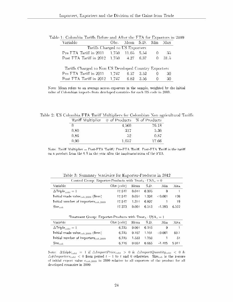
US exports obtain duty-free status after the FTA. Table 1 provides summary statistics for Colombian
tari�s faced by US exporters and a comparable set of exporters from developed countries before
and after the FTA. The pre-FTA tari� for 2011 fell from an average of 11 percentage points to an
average of 4 percentage points in our sample. The tari� elimination was largely on the Colombian
side because 90 percent of US imports from Colombia enjoyed duty free access before the FTA.
The US is Colombia's leading trade partner and the FTA was a substantial step towards trade
liberalization in Colombia. Between June 2012 and April 2013, US exports to Colombia increased
by 14.2 percent over the same period a year earlier while total Colombian imports were up only 4.6
percent.
The theoretical predictions of the model focus on the simultaneous rise in prices and drop in
quantities and import partners. An exporter, c, increases the import price of its product (m̃c),
reduces its total quantity (qc) and reduces the number of its importers (dmaxc ). We de�ne the
triple prediction as ∆Triplecsht = 1 if exporter c from source country s selling product h at time t
21
Importers, Exporters and the Division of the Gains from Trade
increases its average price across all its importers (4 ln Import Pricecsht > 0) and reduces the total
quantity sold to all its importers (∆Xcsht < 0) and reduces the number of importers of its product
(∆dmaxcsht < 0). If any one of these events does not happen, then ∆Triplecsht = 0.
To test the theoretical results, we need measures of ∆Triplecsht and the treatment variables. We
use Colombian import transactions data recorded by its customs authority, which lists the name of
the importer and the exporter for each import transaction.9 We clean the names by harmonizing
commonly occurring pre�xes and su�xes and then aggregating imports to the exporter-country-
product level in each time period (csht). A time period consists of the months from June to
November for each year (2009-2012).10 For each time period, import values and quantities are
recorded at the 8-digit level under the Colombian implementation of Harmonized System (HS)
classi�cation. We compute the average import price (unit value in USD), the total quantity, and
the total number of importers for each exporter-country-product-year, csht. We then compute
∆Triplecsht = 1 for exporter-country-products that have a higher average price, lower total quantity
and fewer importers compared to the previous period.
As customs data are known to be noisy, we typically separate the set of exporter-country-
products with initial sales of less than US$10,000 and only include the set of country-product pairs
with more than one exporter in 2009. The theory applies to incumbent exporters, so we focus on
exporters who sell from 2009 to 2012. Pierce and Schott (2012) show that HS codes change over
time and this can lead to estimation bias. To account for this, we work with the set of products
with HS codes that are unchanged between 2009-2012. This covers 84 percent of all products in our
sample, alleviating concerns regarding generality of the results.
To construct the treatment variables, tari� data for the US-Colombia FTA is obtained from the
O�ce of the US Trade Representative. Tari�s were reduced from their initial levels by one of four
FTA multipliers: 0% of the initial tari�, 80% of the initial tari�, 87% of the initial tari� or 90% of
the initial tari�. Table 2 summarizes the distribution of HS-codes by the FTA tari� multiplier. We
classify Treath = 1 for product codes with a Tari� multiplier equal to zero. For all other product
codes, Treath = 0.
4.2 Baseline Empirical Speci�cation
We examine whether the US-Colombia FTA induced US exporters to increase prices, reduce quanti-
ties and reduce the number of importers in Colombia. To control for underlying trends, we examine
whether exporters from the US selling products that started to receive duty-free access into Colom-
bia were more likely to increase their prices, reduce their quantities and reduce their number of
9The raw data come from www.importgenius.com.10 The interval starts in June since the FTA came into force in the middle of May 2012. The period ends in
November since data for December 2011 are missing. We also do not have data for July 2009 and quantities havebeen appropriately scaled to account for this. Results are robust to using 2010 as the initial period (available uponrequest).
22

Importers, Exporters and the Division of the Gains from Trade
importers relative to the previous period. We de�ne Postt = 1 for the period after the FTA and
0 for the period before the FTA. In addition, we compare the probabilities for US exporters to a
control group of exporters that did not experience the FTA tari� reduction. We focus on exporters
from developed countries to construct a suitable control group. Accordingly, USAs = 1 for exporters
from the United States and 0 for exporters from any other developed country.
Table 3 summarizes the triple dummy and exporter characteristics for exporters in the control
and the treatment groups separately for 2012. As expected, the triple prediction is more prevalent
for the treatment group, but this could be due to di�erences in product composition or due to other
events speci�c to the post-FTA time period. In order to minimize these concerns, we proceed to a
di�erence-in-di�erence estimation which accounts for product-speci�c and country-speci�c e�ects.
We examine the prevalence of simultaneous increases in prices, reductions in quantities and
reductions in the number of importers of an exporter. The estimating equation for the triple
prediction for exporter c from source country s selling product h at time t is a linear probability
model,
∆Triplecsht =β · Postt · Treath ·USAs + γXcsht + αst + αht + εcsht (7)
where εcsht is a disturbance term while αst and αht are source country-year and product-year �xed
e�ects that account for changes such as exchange rate �uctuations and aggregate demand shocks.
Xcsht includes all interactions between Postt, Treath, and USAs, and other controls such as pre-
trends and their interactions (where Pret = 1 for observations in 2011 and 0 otherwise). The
coe�cient of interest is β which we expect to be positive if the FTA led exporters to consolidate
their import market resulting in higher import prices, lower import quantities and fewer importers.
From the theoretical results in Section 3, we expect the triple prediction to vary across exporters
of di�erent levels of productivity. High productivity exporters are expected to have already paid
the costs of consolidating their import market, so bilateral trade liberalization would lead to consol-
idation in the import markets of less productive exporters from the US. To account for di�erences
in responses across exporters, we allow the coe�cient on Postt ·Treath ·USAs to vary with exporter
size. For each exporter-country-product observation, exporter size is measured by the z-score of the
initial value of sales of the exporter in 2009, relative to all exporters of the product from developed
countries in 2009. Let ecsh,2009 denote the initial value of sales of exporter c from country s of prod-
uct h in 2009. The z-score of initial size is Sizecsh ≡ (ecsh,2009 − µh,2009) /σh,2009 which measures
the initial sales of an exporter relative to exporters of that product from all developed countries.11
Accounting for possible di�erential responses across �rms, the estimating equation is
∆Triplecsht =β · Postt · Treath ·USAs + β1 · Postt · Treath ·USAs · Sizecsh + γXcsht + αst + αht + εcsht(8)
11µh,2009 is the mean of ecsh,2009 across all exporters of product h from developed countries and σh,2009 is thecorresponding standard deviation.
23
Importers, Exporters and the Division of the Gains from Trade
Table 1: Colombia Tari�s Before and After the FTA for Exporters in 2009Variable Obs. Mean S.D. Min Max
Tari�s Charged to US Exporters
Pre-FTA Tari� in 2011 1,750 11.05 5.54 0 35
Post-FTA Tari� in 2012 1,750 4.27 6.37 0 31.5
Tari�s Charged to Non-US Developed Country Exporters
Pre-FTA Tari� in 2011 1,747 6.57 3.52 0 30
Post-FTA Tari� in 2012 1,747 6.82 3.56 0 30
Note: Mean refers to an average across exporters in the sample, weighted by the initialvalue of Colombian imports from developed countries for each HS code in 2009.
Table 2: US-Colombia FTA Tari� Multipliers for Colombian Non-agricultural Tari�sTari� Multiplier # of Products % of Products
0 4,560 76.18
0.80 317 5.30
0.86 52 0.87
0.90 1,057 17.66
Note: Tari� Multiplier = Post-FTA Tari�/ Pre-FTA Tari�. Post-FTA Tari� is the tari�on a product from the US in the year after the implementation of the FTA
Table 3: Summary Statistics for Exporter-Products in 2012Control Group: Exporter-Products with Treath ·USAs = 0
Variable Obs (csht) Mean S.D. Min Max
∆Triplecsht = 1 17,547 0.044 0.205 0 1
Initial trade valuecsh,2009 ($mn) 17,547 0.054 1.298 <0.001 126
Initial number of importerscsh,2009 17,547 1.314 0.897 1 19
Sizecsh 17,373 0.004 0.513 -1.593 6.522
Treatment Group: Exporter-Products with Treath ·USAs = 1
Variable Obs (csht) Mean S.D. Min Max
∆Triplecsht = 1 6,225 0.064 0.245 0 1
Initial trade valuecsh,2009 ($mn) 6,225 0.107 1.101 <0.001 60.1
Initial number of importerscsh,2009 6,225 1.533 1.703 1 54
Sizecsh 6,116 0.052 0.665 -1.485 5.911
Note: ∆Triplecsht = 1 if 4ImportPricecsht > 0 & 4ImportQuantitycsht < 0 &4#Importerscsht < 0 from period t − 1 to t and 0 otherwise. Sizecsh is the z-scoreof initial export value ecsh,2009 in 2009 relative to all exporters of the product for alldeveloped countries in 2009.
24

Importers, Exporters and the Division of the Gains from Trade
where Xcsht includes interactions of Sizecsh with Postt, Treath, USAs and Pret as well. Coe�cient
β1 allows the impact of the FTA liberalization to vary by initial size of the exporter. We cluster
standard errors for each estimating equation by exporter-country pairs to account for correlation
across time and products within an exporter-country pair.
4.3 Baseline Results
Table 4 summarizes the results from estimation of the linear probability models in Equations 7 and
8.
4.3.1 Baseline Speci�cation
Column (1) shows that exporters who experienced duty-free access from the US-Colombia FTA
are more likely to increase their average price, reduce their total quantities and sell through fewer
importers, relative to a control group of developed country exporters who did not experience duty-
free access for the product. The likelihood of a triple for the treated exporters rises 1.5 percentage
points more after the FTA relative to the change for other exporters.
4.3.2 Triple Prediction by Exporter Type
Column (2) adds the interaction with the initial size of the exporter. From the theory, the sign
of the interaction term is expected to be negative as less productive exporters are more likely to
consolidate their import market after the FTA. The results in Column (2) show that exporters with
smaller initial size are indeed more likely to consolidate their import market. Figure 2 plots the
histogram of the estimated impact of the FTA across all exporters, β̂0 · Postt · Treath ·USAs + β̂1 ·Postt ·Treath ·USAs ·Sizecsh. Most of the exporters from the US have an increase in the probability
of higher prices, lower quantities and fewer partners as a result of the liberalization.
Another way of capturing the di�erences in the triple prediction is to estimate the treatment
coe�cient separately for exporters of di�erent sizes. Instead of using a continuous measure of initial
size, we estimate di�erent coe�cients for exporters by their size category. We divide all exporters of
a product into di�erent size bins and estimate separate coe�cients on Postt ·Treath ·USAs for eachsize bin. Among exporters that earn over USD10,000 per time period, Tercile1csh = 1 if exporter
c's initial size measured by Sizecsh is below the 33rd percentile of all exporters of that product from
developed countries, and 0 otherwise. Similarly, Tercile2csh = 1 if c's initial size is between the
33rd and 66th percentile, and Tercile3csh = 1 if c's initial size is greater than the 66th percentile
for exporters of that product. We separate the Tiny exporter-country-products with initial sales
less than US$10,000 into another size bin (Tinycsh = 1ecsh,2009≤10000). Column (1) of Table 5 shows
that the triple prediction continues to hold and it is the medium-sized exporters in the �rst and
second terciles that increase prices, reduce quantities and reduce their number of importers. This is
25
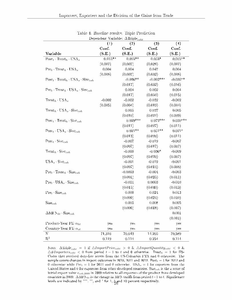
Importers, Exporters and the Division of the Gains from Trade
Table 4: Baseline results: Triple Prediction
Dependent Variable: ∆Triplecsht(1) (2) (3) (4)
Coef. Coef. Coef. Coef.
Variable (S.E.) (S.E.) (S.E.) (S.E.)
Postt · Treath ·USAs 0.015** 0.015** 0.053* 0.015**
(0.007) (0.007) (0.028) (0.007)
Pret · Treath ·USAs 0.004 0.004 0.047 0.004
(0.008) (0.007) (0.032) (0.008)
Postt · Treath ·USAs · Sizecsh -0.036** -0.092*** -0.036**
(0.017) (0.032) (0.016)
Pret · Treath ·USAs · Sizecsh 0.004 0.002 0.004
(0.017) (0.050) (0.015)
Treath ·USAs -0.002 -0.002 -0.022 -0.002
(0.005) (0.004) (0.019) (0.004)
Treath ·USAs · Sizecsh 0.005 0.027 0.005
(0.010) (0.024) (0.009)
Postt · Treath · Sizecsh 0.029*** 0.072*** 0.030***
(0.011) (0.027) (0.011)
Postt ·USAs · Sizecsh 0.021** 0.051** 0.021*
(0.013) (0.020) (0.011)
Postt · Sizecsh -0.007 -0.019 -0.007
(0.007) (0.017) (0.007)
Treath · Sizecsh -0.009 -0.036* -0.009
(0.007) (0.020) (0.007)
USAs · Sizecsh -0.001 -0.019 -0.001
(0.007) (0.014) (0.008)
Pret · Treath · Sizecsh -0.0003 -0.004 -0.003
(0.001) (0.025) (0.011)
Pret ·USAs · Sizecsh -0.011 0.0003 -0.010
(0.015) (0.040) (0.013)
Pret · Sizecsh 0.009 0.024 0.013
(0.009) (0.024) (0.010)
Sizecsh 0.005 0.008 0.005
(0.006) (0.018) (0.007)
∆MFNht · Sizecsh 0.001
(0.001)
Product-Year FE αht yes yes yes yes
Country-Year FE αst yes yes yes yes
N 71,316 70,643 14,205 70,589
R2 0.119 0.114 0.254 0.114
Note: ∆Triplecsht = 1 if 4ImportPricecsht > 0 & 4ImportQuantitycsht < 0 &4#Importerscsht < 0 from period t − 1 to t and 0 otherwise. Treath = 1 for HS-Codes that received duty-free access from the US-Colombia FTA and 0 otherwise. Thesample covers changes in import outcomes in 2010, 2011 and 2012. Postt = 1 for 2012 and0 otherwise while Pret = 1 for 2011 and 0 otherwise. USAs = 1 for exporters from theUnited States and 0 for exporters from other developed countries. Sizecsh is the z-score ofinitial export value ecsh,2009 in 2009 relative to all exporters of the product from developedcountries in 2009. ∆MFNht is the change in MFN tari�s from period t−1 to t. Signi�cancelevels are indicated by ∗∗∗, ∗∗, and ∗ for 1, 5 and 10 percent respectively.
26

Importers, Exporters and the Division of the Gains from Trade
Figure 2: Distribution of Estimated Treatment E�ects in 2012
020
4060
Per
cent
age
of T
reat
ed U
S E
xpor
ter-
Pro
duct
Pai
rs
-.2 -.15 -.1 -.05 0 .05Estimated Treatment Effect by Initial Size of Treated US Exporter-Product Pairs
Note: Horizontal axis shows the magnitude of the estimated treatment e�ect.
consistent with the theory because the most and least productive exporters do not switch contracts
and it is the medium productivity exporters that switch from bilateral to joint contracts. The
coe�cient on the second tercile is less precisely estimated, and the pre-treatment variables are
always statistically insigni�cant. It is also reassuring that tiny exporters show the opposite results
which suggests that it is not purely selection e�ects at the bottom end of the exporter distribution
that drives the results. Theoretically, the selection e�ects would work to increase exports of the
tiny exporters. Column (2) of Table 5 shows that the triple prediction holds when tari�-inclusive
prices are used instead of free-on-board (FOB) prices. So the rise in import prices is large enough
to o�set the direct impact of a reduction in tari�s after the FTA.
One shortcoming of measuring consolidation in the import market through the ∆Triplecsht in-
dicator is that it will always be zero for exporters that sell to only one importer in the previous
period. This underestimates the relative prevalence of the triple prediction among the set of ex-
porters that sell to more than one importer initially. Column (3) restricts the estimation sample to
exporter-country-products with more than one import partner initially. As expected, the coe�cient
on Postt · Treath · USAs increases to over 5 percentage points.12 Exporters who gained duty-free
access from the FTA are more likely to increase prices, lower quantities and sell to fewer importers.
This e�ect varies across exporters of di�erent initial size with smaller exporters more likely to engage
12Another concern might be that the higher prevalence of the triple prediction could be due to an increase in thevariance of price changes, quantity changes and changes in the number of importers. While increases in the variancesof these outcomes is consistent with the theory, we also re-estimate the regressions controlling for changes in thevariances. The main results are unchanged but our sample is smaller because computing changes in variances for theUS and other developed countries separately is more demanding on the data (available upon request).
27

Importers, Exporters and the Division of the Gains from Trade
Table 5: Tercile results: Triple Prediction and Unit Value Changes by Size Bins∆Triplecsht ∆ ln Import Pricecsht
(1) fob (2) w/tari� (3) fob (4) w/tari�
Coef. Coef. Coef. Coef.
Variable (S.E.) (S.E.) (S.E.) (S.E.)
Tercile3csh · Postt · Treath ·USAs -0.021 -0.031 -0.025 -0.069
(0.021) (0.022) (0.104) (0.104)
Tercile2csh · Postt · Treath ·USAs 0.043 0.037 0.084* 0.040
(0.027) (0.024) (0.133) (0.133)
Tercile1csh · Postt · Treath ·USAs 0.077*** 0.068** 0.314** 0.257*
(0.024) (0.027) (0.139) (0.139)
Tinycsh · Postt · Treath ·USAs -0.067 ** -0.064** -0.353** -0.347**
(0.027) (0.028) (0.149) (0.149)
Controls (including Pre-treatment) yes yes yes yes
Product-Year FE αht yes yes yes yes
Country-Year FE αst yes yes yes yes
N 71,316 71,316 71,316 71,285
R2 0.121 0.117 0.089 0.089
Note: ∆Triplecsht = 1 if 4ImportPricecsht > 0 & 4ImportQuantitycsht < 0 &4#Importerscsht < 0 from period t − 1 to t and 0 otherwise. ∆ ln Import Pricecshtis the log change in the exporter-level average unit value. Columns (1) and (3) use FOBprices and Columns (2) and (4) use prices inclusive of e�ective duty rates. Treath = 1for HS-Codes that received duty-free access from the US-Colombia FTA and 0 otherwise.The sample covers changes in import outcomes in 2010, 2011 and 2012. Postt = 1 for2012 and 0 otherwise while Pret = 1 for 2011 and 0 otherwise. USAs = 1 for exportersfrom the United States and 0 for exporters from other developed countries. Sizecsh is thez-score of initial export value ecsh,2009 in 2009 relative to all exporters of the product fromdeveloped countries in 2009. Tercile1csh = 1 for the 33rd tercile of Sizecsh, Tercile2csh = 1for the 66th tercile and Tercile3csh = 1 for the top tercile. Tinycsh = 1 for all exportersfrom developed countries with total sales of less than USD10,000 in 2009. Controls in-clude all interactions between Postt, Treath, USAs, Pret and indicators for initial size bins.Signi�cance levels are indicated by ∗∗∗, ∗∗, and ∗ for 1, 5 and 10 percent respectively.
28
Importers, Exporters and the Division of the Gains from Trade
in consolidation of their import markets.
4.3.3 Quantitative Interpretation
An advantage of testing the model with the triple prediction is that it lets us examine a unique
prediction which does not arise in standard models. A limitation of the triple prediction however is
that it does not let us put a number on the price increases faced by the importers. To get a sense
of the magnitude of the changes, we examine how unit values respond to duty-free access to the
Colombian market.
Using a speci�cation similar to the baseline, we regress changes in unit values to determine
the coe�cient on Postt · Treath · USAs for each tercile of US exporters. The dependent variable
in Column (3) of Table 5 reports the change in the average FOB price charged by exporter c for
product h and Column (4) reports the change in the tari�-inclusive price where the tari� is the
MFN or preferential average applied duty rate. As earlier, tiny exporters and large exporters (in
the third tercile) reduce their prices. From the theory, these are the �rms that will not switch
contracts after trade liberalization and their decisions will reinforce the standard gains from trade.
Medium-size importers (in the �rst and second terciles of initial size greater than $10,000) show
the opposite e�ect. These are the �rms that are expected to consolidate their import market by
switching to joint contracts. And we �nd that they indeed increase their prices between 8 to 30%.
To interpret the price changes, we regress the log change in tari�-inclusive unit values of each
exporter on the indicator for Postt · Treath · USAs for all exporters, without any size conditioning.
The coe�cient is -0.0425 which is estimated imprecisely. This implies that duty-free access to the
Colombian import market induced exporters to reduce their tari�-inclusive prices by 4.25%. This
low pass-through re�ects the fact that the medium-size exporters increase their prices.
Having discussed the baseline results, we examine the robustness of these predictions with a
series of checks on our results.
4.4 Robustness Checks
The robustness checks in this sub-section can be broadly divided into three types. First, we control
for other explanations such as contemporaneous tari� cuts for trade partners to other developed
countries to minimize bias in the baseline estimates from omitted variables. Second, we look at a
quality-based explanations for the triple prediction. Finally, we examine whether the triple predic-
tion continues to hold when we look within exporter-importer pairs.
4.4.1 Multilateral tari� cuts
The time period that we study also includes a unilateral tari� reform in Colombia that reduced
the average tari� from 12.2 percent to 8.2 percent on November 5 2010 (WTO 2012). The stated
29

Importers, Exporters and the Division of the Gains from Trade
aim of this tari� reform was to reduce the dispersion in tari�s and eliminate the negative e�ective
protection that existed in some industries. The reform reduced most-favored-nation (MFN) tari�s
on a subset of products. For products in our sample, the average MFN duty was 10.3 percentage
points before the reform and the duty fell by 1.3 percentage points as a result of the reform.
To account for unilateral changes in Colombia's MFN tari�s, Column (4) of Table 4 includes an
interaction between the change in MFN tari�s and initial size of the exporter. As the MFN tari�
change applies to all trade partners with MFN status, the e�ect of ∆MFNht is subsumed in the
product-time �xed e�ects αht. Across di�erent speci�cations, we �nd that our main �ndings are
una�ected, and the interaction between MFN tari� changes and initial size is small and statistically
insigni�cant for the triple prediction.
4.4.2 Revenue Predictions
Increases in unit values following a trade liberalization are often interpreted as quality upgrading
by exporters (Verhoogen 2008; Khandelwal 2010). Colombia is a small country relative to other
destinations of US exporters, making it less likely that the unit values pick up investments in quality
upgrading of US exporters following duty-free access to the Colombian market. In fact, lower trade
costs would make it more likely for lower quality US exporters to be able to sell to the Colombian
market, because the exporting cost cuto� typically rises after trade liberalization in heterogenous
�rm trade models. Empirically, higher quality products are more likely to be shipped out when trade
barriers are higher (Hummels and Skiba 2004). To ensure however that our results are not driven
by quality increases, we examine another triple prediction which looks at a decline in total revenue
rather than total quantity of the exporter. If the observed price rise is accompanied by a reduction
in revenues and fewer importers, then it is more straightforward to explain it with a reduction in
competition rather than an improvement in quality which would be expected to increase revenues.13
The variety-level model of Section 3 predicts that exporters who switch from bilateral contracts
to joint contracts increase their pro�ts but sell lower quantities to fewer importers. An extreme
prediction of the model is that these exporters might also lower their sales values to earn higher
pro�t margins per unit. The main intuition here is that under joint contracts, the �rm need not
sell many units of the product if the markup is large and the �xed costs of joint versus bilateral
contracts are relatively low. So if we �nd that US exporters are more likely to reduce revenues when
they increase prices and sell to fewer importers, it would be another piece of evidence that duty-free
access induced exporters to increase markups rather than quality.
We examine the revenue-based triple prediction of higher prices, lower revenues and fewer im-
porters in a way similar to the baseline analysis. Speci�cally, ∆TripleRevenuecsht = 1 if exporter c from
source country s selling product h at time t increases its average price across all its importers and
13We are grateful to Penny Goldberg and Marc Melitz for pointing us in this direction.
30

Importers, Exporters and the Division of the Gains from Trade
reduces the total revenue received from all its importers and reduces the number of importers of
its product (dmaxcsht < 0). If any one of these events does not happen, then ∆TripleRevenuecsht = 0. As
in the baseline results, Table 6 shows US exporters who receive duty-free access are more likely to
have higher prices, lower revenues and fewer importers, and these exporters tend to be the smaller
exporters. As expected, the revenue-based triple prediction becomes more likely after the FTA and
its increased likelihood is slightly smaller than that of the quantity-based triple prediction in the
baseline analysis.14
Table 6: Estimation results: Revenue-Based Triple Prediction
Dependent Variable: ∆TripleRevenuecsht
(1) fob (2) w/tari�
Coef. Coef.
Variable (S.E.) (S.E.)
Postt · Treath ·USAs 0.016 ** 0.012*
(0.006) (0.007)
Postt · Treath ·USAs · Sizecsh -0.038*** -0.041***
(0.014) (0.014)
Controls (including Pre-treatment) yes yes
Product-Year FE αht yes yes
Country-Year FE αst yes yes
N 71,316 70,612
R2 0.125 0.113
Note: ∆TripleRevenuecsht = 1 if 4ImportPricecsht > 0 & 4ImportRevenuecsht < 0 &4#Importerscsht < 0 from period t − 1 to t and 0 otherwise. Column (1) uses FOBprices and revenues, and Column (2) uses prices and revenues, inclusive of e�ective dutyrates. Treath = 1 for HS-Codes that received duty-free access from the US-Colombia FTAand 0 otherwise. The sample covers changes in import outcomes in 2010, 2011 and 2012.Postt = 1 for 2012 and 0 otherwise while Pret = 1 for 2011 and 0 otherwise. USAs = 1for exporters from the United States and 0 for exporters from other developed countries.Sizecsh is the z-score of initial export value ecsh,2009 in 2009 relative to all exporters ofthe product from developed countries in 2009. Controls include all interactions betweenPostt, Treath, USAs, Sizecsh and Pret. Signi�cance levels are indicated by ∗∗∗, ∗∗, and ∗
for 1, 5 and 10 percent respectively.
4.4.3 Quality Estimation
To look further into the quality explanation, we estimate quality based on standard methods and
a �exible approach that is consistent with our theory. We show that the triple prediction using
quality-adjusted prices (instead of simple unit values) continues to hold. Exporters who gained
duty-free access became more likely to increase prices, reduce quantities and reduce the number of
their importers, even after adjusting for estimated quality.
14The main results are similar when we only use a double prediction of lower revenue and fewer importers on theHS (available upon request).
31

Importers, Exporters and the Division of the Gains from Trade
Let λc denote the quality of exporter c's variety. Then welfare from the di�erentiated goods is
Q =´λcu(qc)dGc. We are interested in quality-adjusted prices which net out changes in exporter-
level quality λc before and after the trade liberalization. The quality adjusted price is pcd/λc =
v′(qcd)u′(qc)Q
η−1 and we will infer it in two ways. First, we follow Khandelwal et al. (2013) and
use the elasticities of substitution from the literature to recover quality-adjusted prices, based on
the markup assumptions in the theory of Section 2. Then we will discuss a more �exible approach
that enables us to directly approximate the lower nest marginal utility.
For an exporter c that sells to more than one importer d, the inverse demand for the variety is
ln pcd = ln v′(qcd)+(lnλc + lnu′(qc)− (1− η) lnQ) ≡ ln v′(qcd)+αc where αc is an exporter-speci�c
term. We typically have estimates for the elasticity in the upper nest of u(qc) but do not have readily
available measures of the elasticity in the lower nest v(qcd). To make progress, we augment the
approach of Khandelwal et al. (2013) to recover quality using demand elasticities from Broda and
Weinstein (2006) and Soderbery (2015). Assuming v(qcd) ≡ q1−µvcd , ln v′(qcd) = ln (1− µv)−µv ln qcd.
A key assumption in our theory is that the elasticity of demand in the upper nest is smaller than the
elasticity in the lower nest (µuεv < minµv min (1− µv)), so we get a lower bound for the elasticity inthe lower nest. Let the upper nest utility function be CES with a di�erentiation parameter denoted
by 1 − µu. Then we know that the elasticity for the lower nest is bounded below by the upper
nest elasticity so that µv = κµu for 0 < κ < 1, and we will use the upper nest elasticities from the
literature to estimate quality. We estimate the unit value of the variety of exporter-importer cd for
each HS code h from source country s in each time period t as
ln pcdsht = −κ · µuh ln qcdsht + αcsht + εcdsht
where µuh is obtained from Broda-Weinstein-Soderbery elasticities (σh ≡ 1/µuh). The key identi-
fying assumptions are that κ does not vary across products and that quality varies at the exporter-
product-time level. Having estimated κ̂ and α̂csht, we recover quality ln λ̂csht as a residual by
regressing α̂csht + µuh ln qchst − ln (1− µuh) on product-time �xed e�ects and using µuh from the
Broda-Weinstein-Soderbery estimates of elasticities of substitution across product groups. Then
the quality-adjusted prices are ln pcdsht− lnλcsht which we use to determine the changes in quality-
adjusted price in the triple prediction.
Under the �exible approach, we move away from the lower bound method and approximate the
lower nest marginal utility as a function of quantities. The �rst step is to estimate v′(qcd) which
we take to be a cubic function of ln qcd. The unit value of exporter-importer cd for each HS code h
from source country s in each time period t is
ln pcdsht = β1 ln qcdsht + β2 (ln qcdsht)2 + β3 (ln qcdsht)
3 + αcsht + εcdsht.
Having approximated v̂′(qcd) = β̂1 ln qcd + β̂2 (ln qcd)2 + β̂3 (ln qcd)
3, we proceed to recover λc. As-
suming u′(qc) = q1−µuc , our estimated exporter-speci�c quality is lnλcsht + lnαht = ln pcdsht −
32

Importers, Exporters and the Division of the Gains from Trade
ln v̂′(qcdsht) + µuh ln qcsht − ln (1− µuh) which is identi�ed up to a constant and where µuh is based
on Broda-Weinstein-Soderbery estimates of elasticities of substitution for the product group h. De-
tails of the quality estimation are provided in the Appendix and here we discuss the triple prediction
using quality-adjusted prices.
The triple prediction continues to show similar results when quality-adjusted prices are used
instead of unit prices. Column (1) of Table 7 is based on the quality-adjusted prices from the �rst
method and Column (2) is based on the �exible method. We �nd once again that exporters in
terciles 1 and 2 are more likely to consolidate their import market.
Table 7: Tercile results: Quality-adjusted Triple Prediction by Size Bins
Dependent Variable: ∆Triplecsht(1) (2)
Coef. Coef.
Variable (S.E.) (S.E.)
Tercile3csh · Postt · Treath ·USAs 0.001 -0.006
(0.023) (0.023)
Tercile2csh · Postt · Treath ·USAs 0.026 0.019
(0.021) (0.023)
Tercile1csh · Postt · Treath ·USAs 0.071** 0.061**
(0.032) (0.030)
Tinycsh · Postt · Treath ·USAs -0.063** -0.056*
(0.031) (0.030)
Controls (including Pre-treatment) yes yes
Product-Year FE αht yes yes
Country-Year FE αst yes yes
N 57,480 57,480
R2 0.112 0.124
Note: ∆Triplecsht = 1 if 4QualityAdjImportPricecsht > 0 & 4ImportQuantitycsht < 0& 4#Importerscsht < 0 from period t− 1 to t and 0 otherwise. Treath = 1 for HS-Codesthat received duty-free access from the US-Colombia FTA and 0 otherwise. The samplecovers changes in import outcomes in 2010, 2011 and 2012. Postt = 1 for 2012 and 0otherwise while Pret = 1 for 2011 and 0 otherwise. USAs = 1 for exporters from theUnited States and 0 for exporters from other developed countries. Sizecsh is the z-score ofinitial export value ecsh,2009 in 2009 relative to all exporters of the product from developedcountries in 2009. Tercile1csh = 1 for the 33rd tercile of Sizecsh, Tercile2csh = 1 for the 66thtercile and Tercile3csh = 1 for the top tercile. Tinycsh = 1 for all exporters from developedcountries with total sales of less than USD10,000 in 2009. Controls include all interactionsbetween Postt, Treath, USAs, Pret and indicators for initial size bins. Standard errors arebootstrapped and clustered by exporter. Signi�cance levels are indicated by ∗∗∗, ∗∗, and∗ for 1, 5 and 10 percent respectively.
4.4.4 Within-Exporter-Importer Pairs
While the baseline results examine the triple prediction at the level of the exporter, the model
predicts that the results should also hold for some exporter-importer pairs so we estimate the triple
33

Importers, Exporters and the Division of the Gains from Trade
prediction at the exporter-importer pair level. Let d denote a Colombian importer that imports
from exporter c. The triple variable is now de�ned as ∆Triplecdsht = 1 for exporter-importer pairs
cd that experience an increase in their bilateral price, a fall in their bilateral quantity (∆qcdsht < 0)
and a decrease in the importers that buy from c (∆dmaxcsht < 0). If any one of these events does not
happen, then ∆Triplecdsht = 0. Columns (1) and (2) of Table 8 show that the likelihood of increasing
import prices, reducing quantities and reducing the number of importers goes up after the trade
liberalization. As earlier, exporter-importer pairs in the middle of the exporter size distribution are
more likely to see the triple prediction hold. The exporter-importer pairs of tiny and large exporters
who are not expected to switch contracts show small e�ects or a reduction in the likelihood of the
triple prediction.
Table 8: Exporter-Importer results: Triple Prediction Within Exporter-Importer Pairs
Dependent Variable: ∆Triplecdsht(1) fob (2) w/tari�
Coef. Coef.
Variable (S.E.) (S.E.)
Tercile3csh · Postt · Treath ·USAs -0.005 -0.017
(0.025) (0.025)
Tercile2csh · Postt · Treath ·USAs 0.046* 0.028
(0.028) (0.027)
Tercile1csh · Postt · Treath ·USAs 0.053** 0.051**
(0.026) (0.026)
Tinycsh · Postt · Treath ·USAs -0.0414 -0.049*
(0.028) (0.027)
Controls (inc. Pre-treatment) yes yes
Product-Year FE αht yes yes
Country-Year FE αst yes yes
N 82,130 82,130
R2 0.110 0.106
Note: ∆Triplecdsht = 1 if 4ImportPricecdsht > 0 & 4ImportQuantitycdsht < 0 &4#Importerscsht < 0 from period t − 1 to t and 0 otherwise. Column (1) uses FOBprices and Column (2) uses prices inclusive of e�ective duty rates. Treath = 1 for HS-Codes that received duty-free access from the US-Colombia FTA and 0 otherwise. Thesample covers changes in import outcomes in 2010, 2011 and 2012. Postt = 1 for 2012 and0 otherwise while Pret = 1 for 2011 and 0 otherwise. USAs = 1 for exporters from theUnited States and 0 for exporters from other developed countries. Sizecsh is the z-score ofinitial export value ecsh,2009 in 2009 relative to all exporters of the product from developedcountries in 2009. Tercile1csh = 1 for the 33rd tercile of Sizecsh, Tercile2csh = 1 for the66th tercile and Tercile3csh = 1 for the top tercile. Tinycsh = 1 for all exporters fromdeveloped countries with total sales of less than USD10,000 in 2009. Controls includeall interactions between Postt, Treath, USAs, Pret and indicators for initial size bins.Signi�cance levels are indicated by ∗∗∗, ∗∗, and ∗ for 1, 5 and 10 percent respectively.
34

Importers, Exporters and the Division of the Gains from Trade
5 Conclusion
This paper examines how the microstructure of import markets a�ects the division of the gains from
trade among consumers, importers and exporters. When an exporter sells a product to importers
through anonymous markets, double marginalization and business stealing among competing im-
porters lead to lower pro�ts. Exporters and importers can invest in relationships that overcome
these sources of lower pro�ts.
We embed the choice of contracts between exporters and importers into a trade model with
heterogeneous exporters and importers. Exporters can o�er bilateral contracts that eliminate dou-
ble marginalization, leading to higher pro�ts and lower prices. Exporters can internalize business
stealing across importers by investing in joint contracts. This enables an exporter to commit to
mitigating competition among its importers to maximize nultilateral pro�ts. When investments in
joint contracts embody economies of scale and markups rise with quantities, trade liberalization
changes the relative incentives to engage in bilateral contracts and joint contracts. Lower trade
costs increase the surplus from joint contracts, and this change in the microstructure of the import
market increases �rm pro�ts at the expense of consumer welfare.
The model enables us to derive unique predictions for changes in import prices, quantities
and the number of importers per exporter. Testing these implications empirically, we show that
bilateral trade liberalization between Colombia and the US induced US exporters to consolidate their
import market, increasing the probability of higher prices, reduced quantity and fewer Colombian
importers per exporter. These observable predictions suggest that the actions of exporters and
importers a�ect the ability of consumers to gain from trade. The estimated elasticity of import
prices with respect to trade costs shows substantial increases in prices for certain products from trade
liberalization. Future work can shed more light on how this translates into consumer price changes
and its contribution to the aggregate pass-through of reduction in trade barriers into consumer
prices.
References
Ahn, J., A. K. Khandelwal, and S. Wei (2011): �The role of intermediaries in facilitating
trade,� Journal of International Economics, 84(1), 73�85. 1
Akerman, A. (2010): �A theory on the role of wholesalers in International trade based on economies
of scope,� Research papers in economics, Stockholm University, Department of Economics. 1
Amiti, M. and J. Konings (2007): �Trade Liberalization, Intermediate Inputs and Productivity:
Evidence from Indonesia,� American Economic Review, 97, 1611�1638. 1
35

Importers, Exporters and the Division of the Gains from Trade
Antràs, P. and A. Costinot (2011): �Intermediated Trade,� The Quarterly Journal of Eco-
nomics, 126, 1319�1374. 1
Antràs, P. and E. Helpman (2004): �Global Sourcing,� Journal of Political Economy, 112,
552�580. 1
Atkin, D. and D. Donaldson (2012): �Who's Getting Globalized? The Size and Nature of
Intranational Trade Costs,� Working Paper. 1
Badinger, H. (2007): �Has the EU's Single Market Programme Fostered Competition? Testing
for a Decrease in Mark-up Ratios in EU Industries,� Oxford Bulletin of Economics and Statistics,
69, 497�519. 1, 1
Bagwell, K. and S. H. Lee (2015): �Trade Policy under Monopolistic Competition with Firm
Selection,� Wokirng Paper, Stanford University. 1
Bagwell, K. and R. W. Staiger (2012): �The economics of trade agreements in the linear
Cournot delocation model,� Journal of International Economics, 88, 32�46. 1
Baller, S. (2013): �Product quality, market size and welfare: theory and evidence from French
exporters,� Working Paper University of Oxford. 3.1
Bernard, A. B., J. B. Jensen, S. J. Redding, and P. K. Schott (2010): �Wholesalers and
Retailers in US Trade,� The American Economic Review, 100, 408�413. 1
Bernard, A. B., J. B. Jensen, and P. K. Schott (2009): �Importers, Exporters, and Multina-
tionals: A Portrait of Firms in the U.S. that Trade Goods,� in Producer dynamics: New Evidence
from Micro Data, ed. by T. Dunne, J. Jensen, and M. Roberts, University of Chicago Press. 1
Bernard, A. B., A. Moxnes, and K. H. Ulltveit-Moe (2014): �Two-sided Heterogeneity and
Trade,� Working Paper 20136, NBER. 1, 7
Blanchard, E., T. Chesnokova, and G. Willmann (2013): �Private labels and international
trade: Trading variety for volume,� Tech. rep., Kiel Working Paper. 1
Blum, B. S., S. Claro, and I. Horstmann (2010): �Facts and �gures on intermediated trade,�
The American Economic Review, 100, 419�423. 1
Blum, B. S., S. Claro, and I. J. Horstmann (2012): �Import Intermediaries and Trade Costs:
Theory and Evidence,� mimeo, University of Toronto. 1
Boler, E. A., A. Moxnes, and K. H. Ulltveit-Moe (2015): �Technological Change, Interna-
tional Sourcing and the Joint Impact on Productivity,� American Economic Review, 105, 3704�39.
1
36

Importers, Exporters and the Division of the Gains from Trade
Broda, C. and D. E. Weinstein (2006): �Globalization and the Gains From Variety,� The
Quarterly Journal of Economics, 121, 541�585. 4.4.3
Burstein, A. T., J. C. Neves, and S. Rebelo (2003): �Distribution costs and real exchange
rate dynamics during exchange-rate-based stabilizations,� Journal of monetary Economics, 50,
1189�1214. 1
Campa, J. M. and L. S. Goldberg (2005): �Exchange Rate Pass-Through into Import Prices,�
The Review of Economics and Statistics, 87, 679�690. 1
Carballo, J., G. I. Ottavianio, and C. V. Martincus (2013): �The Buyer Margins of Firms'
Exports,� Tech. rep., LSE. 1
Castellani, D., F. Serti, and C. Tomasi (2010): �Firms in international trade: Importers' and
exporters' heterogeneity in Italian manufacturing industry,� The World Economy, 33, 424�457. 1
Chaney, T. (2014): �The Network Structure of International Trade,� American Economic Review,
104 (11), 3600�3634. 1
Conconi, P., P. Legros, and A. F. Newman (2012): �Trade liberalization and organizational
change,� Journal of international economics, 86, 197�208. 1
De Loecker, J., P. K. Goldberg, A. K. Khandelwal, and N. Pavcnik (2012): �Prices,
markups and trade reform,� Tech. rep., National Bureau of Economic Research. 1, 1
Dhingra, S. and J. M. Morrow (2012): �Monopolistic Competition and Optimum Product
Diversity under Firm Heterogeneity,� Working Paper. 1, 2, 2.1, 2.1
Eaton, J., M. Eslava, D. Jinkins, C. J. Krizan, and J. Tybout (2014): �A Search and
Learning Model of Export Dynamics,� working paper. 1
Eckel, C. (2009): �International trade and retailing,� Working Paper 2597, CESIfo. 1
Eckel, C., L. Iacovone, B. Javorcik, and J. P. Neary (2015): �Multi-product �rms at
home and away: Cost-versus quality-based competence,� Journal of International Economics, 95,
216�232. 3.1
Engel, C. and J. H. Rogers (1996): �How Wide Is the Border?� American Economic Review,
86, 1112�25. 1
Feenstra, R. C., D.-S. Huang, and G. G. Hamilton (2003): �A market-power based model
of business groups,� Journal of Economic Behavior & Organization, 51, 459�485. 1
37

Importers, Exporters and the Division of the Gains from Trade
Fieler, A. C., M. Eslava, and D. Y. Xu (2014): �Trade, Technology and Input Linkages: A
Theory with Evidence from Colombia,� . 1
Ganslandt, M. and K. E. Maskus (2004): �Parallel imports and the pricing of pharmaceutical
products: evidence from the European Union,� Journal of health economics, 23, 1035�1058. 1
Halpern, L., M. Koren, and A. Szeidl (2015): �Imported Inputs and Productivity,� American
Economic Review, 12, 3660�3703. 1
Harrison, A. E. (1994): �Productivity, Imperfect Competition, and Trade Reform: Theory and
Evidence,� Journal of International Economics, 36 (1-2), 53�73. 1
Harrison, R., J. Jaumandreu, J. Mairesse, and B. Peters (2005): �Does Innovation Stim-
ulate Employment? A Firm-level Analysis Using Comparable Micro Data on Four European
Countries,� European research project Innovation and Employment in European Firms: Microe-
conometric Evidence (IEEF). 1
Hart, O. and J. Tirole (1990): �Vertical integration and market foreclosure,� Brookings papers
on economic activity. Microeconomics, 1990, 205�286. 1, 2.4
Horn, H. and A. Wolinsky (1988): �Bilateral monopolies and incentives for merger,� The RAND
Journal of Economics, 408�419. 2.4, 2.5.1
Hummels, D. and A. Skiba (2004): �Shipping the Good Apples Out? An Empirical Con�rmation
of the Alchian-Allen Conjecture,� Journal of Political Economy, 112, 1384�1402. 4.4.2
Khandelwal, A. K. (2010): �The Long and Short (of) Quality Ladders,� Review of Economic
Studies, 77, 1450�1476. 4.4.2
Khandelwal, A. K., P. K. Schott, and S.-J. Wei (2013): �Trade Liberalization and Embedded
Institutional Reform: Evidence from Chinese Exporters,� The American Economic Review, 103,
2169�2195. 4.4.3, 3
Konings, J., P. V. Cayseele, and F. Warzynski (2005): �The E�ects of Privatization and
Competitive Pressure on Firms' Price-Cost Margins: Micro Evidence from Emerging Economies,�
The Review of Economics and Statistics, 87, 124�134. 1
Krugman, P. (1979): �Increasing Returns, Monopolistic Competition, and International Trade,�
Journal of International Economics, 9, 469�479. 2, 2.1
Krugman, P. R. (1980): �Scale Economies, Product Di�erentiation, and the Pattern of Trade,�
American Economic Review, 70, 950�959. 2.2
38

Importers, Exporters and the Division of the Gains from Trade
Lawrence, R. Z. (1991): �How open is Japan?� in Trade with Japan: has the door opened wider?,
University of Chicago Press, 1991, 9�50. 1
Lawrence, R. Z. and G. R. Saxonhouse (1991): �E�cient or exclusionist? The import behavior
of Japanese corporate groups,� Brookings Papers on Economic Activity, 311�341. 1
Levinsohn, J. (1993): �Testing the imports-as-market-discipline hypothesis,� Journal of Interna-
tional Economics, 35, 1�22. 1
Mallick, S. and H. Marques (2008): �Passthrough of Exchange Rate and Tari�s into Import
Prices of India: Currency Depreciation versus Import Liberalization*,� Review of International
Economics, 16, 765�782. 1, 1
Martin, S., H.-T. Normann, and C. M. Snyder (2001): �Vertical foreclosure in experimental
markets,� RAND Journal of Economics, 466�496. 3, 5
Mayer, T., M. J. Melitz, and G. I. Ottaviano (2014): �Market Size, Competition, and the
Product Mix of Exporters,� American Economic Review, 104(2). 1, 2.1
Melitz, M. J. (2003): �The Impact of Trade on Intra-Industry Reallocations and Aggregate In-
dustry Productivity,� Econometrica, 71, 1695�1725. 2.1
Miklos-Thal, J., P. Rey, and T. Verge (2010): �Vertical relations,� International Journal of
Industrial Organization, 28, 345�349. 2
Mollers, C., H.-T. Normann, and C. M. Snyder (2014): �Communication in Vertical Markets:
Experimental Evidence,� Dartmouth College Working Paper. 3
Muuls, M. and M. Pisu (2009): �Imports and Exports at the Level of the Firm: Evidence from
Belgium,� The World Economy, 32, 692�734. 1
Neary, J. P. and M. Mrazova (2013): �Not so demanding: Preference structure, �rm behavior,
and welfare,� Tech. rep., University of Oxford, Department of Economics. 1, 2.1
Parenti, M., P. Ushchev, and J.-F. Thisse (2014): �Toward a theory of monopolistic compe-
tition,� . 1, 2.1
Petropoulou, D. (2011): �Information costs, networks and intermediation in international trade,�
Globalization and Monetary Policy Institute Working Paper 76, Federal Reserve Bank of Dallas.
1
Pierce, J. R. and P. K. Schott (2012): �Concording US Harmonized System Categories over
Time,� Journal of O�cial Statistics, 28, 53�68. 4.1
39

Importers, Exporters and the Division of the Gains from Trade
Raff, H. and N. Schmitt (2005): �Endogenous vertical restraints in international trade,� Euro-
pean Economic Review, 49, 1877�1889. 1
��� (2009): �Buyer Power in International Markets,� Journal of International Economics, 79(2),
222�229. 1
��� (2012): �Imports and the Structure of Retail Markets,� Canadian Journal of Economics,
45(4), 1431�1455. 1
Rauch, J. E. (1999): �Networks versus markets in international trade,� Journal of International
Economics, 48, 7�35. 1
Rauch, J. E. and J. Watson (2004): �Network Intermediaries in International Trade,� Journal
of Economics & Management Strategy, 13, 69�93. 1
Rey, P. and J. Tirole (2007): �A primer on foreclosure,� Handbook of industrial organization, 3,
2145�2220. 2.4
Soderbery, A. (2015): �Estimating import supply and demand elasticities: Analysis and implica-
tions,� Journal of International Economics, 96, 1�17. 4.4.3
Tybout, J. R. (2003): �Plant-and �rm-level evidence on "new" trade theories,� Handbook of
International Trade, 1, 388�415. 1
Venables, A. J. (1985): �Trade and trade policy with imperfect competition: The case of identical
products and free entry,� Journal of International Economics, 19, 1�19. 1
Verhoogen, E. A. (2008): �Trade, Quality Upgrading, and Wage Inequality in the Mexican
Manufacturing Sector*,� The Quarterly Journal of Economics, 123, 489�530. 4.4.2
WTO (2012): �Trade Policy Review: Colombia,� WT/TPR/S/265. 4.4.1
Yeats, A. J. (1978): �Monopoly power, barriers to competition and the pattern of price di�erentials
in international trade,� Journal of Development Economics, 5, 167�180. 1
40

Importers, Exporters and the Division of the Gains from Trade
For Online Publication: Appendix
Fixed Entry
We will show that the pro�ts of the exporters are supermodular in market size and contracting
choice under conditions on the rate at which markups change with quantities.
The exporter's optimal pro�t is πc = s (m(q)q/(1−m(q)))MdβcdL where the markup ism(q) ≡µv(q) + zµu (Mdv(q)) εv(q) for z ∈ {0, 1} at the optimally chosen quantity q. This formulation lets
us specify the di�erent contracting choices through z. Pro�ts under bilateral contracts correspond
to z = 0 and pro�ts under joint contracts correspond to z = 1. The optimal quantity is de-
termined by u′ (Mdv(q)) v′(q) (1−m) = δcd. The consumer budget multiplier is taken as �xed
by the �rm and is given by δ = sMcMdu′ (Mdv(q)) v′(q) in equilibrium. As z rises, the pro�t
function changes by d lnπd ln z =
(1 +
mqqm(1−m)
)d ln qd ln z + zµuεv
m(1−m) . From the optimal pricing condition,
ln δ+lnu′ (Mdv(q)) v′(q) (1− µv − zµuεv) = cd so that −(µ+ µuε+
mqq1−m
)d ln qd ln z = zµuεv
1−m and quan-
tities fall under joint contracts. Substituting in the pro�t derivative, πz = βLτcd (1−z)q(1−m)2
sMd(µuεv)2
µv+µuεv+mqq
1−m
so sπzs/πz = 1 + d ln qd ln s
(1 + 2d lnµuεv
d ln q +2mqq1−m −
d ln(µv+µuεv+mqq
1−m)d ln q
)≡ 1 + (1 +Aq)
d ln qd ln s .
From optimal contracting, πz = βLτcd (1−z)q(1−m)2
xMd(µuεv)2
µv+µuεv+mqq
1−m= fJc so that di�erentiating with re-
spect to market size gives 1 + (1 +Aq)d ln qd ln s + (Az − z/(1− z)) d ln z
ds = 0 for Az ≡ 2zµuε1−m −
d ln( mqq1−m)d ln z .
From optimal pricing and the budget multiplier, 1−m = sqMcMdcd implying −(
1 +mqq1−m
)d ln qd ln s −
zµuεv1−m
d ln zd ln s = 1. Putting the two together, −
(1 +
mqq1−m +
zµuεv1−m (1+Aq)
z1−z−Az
)(d ln q/d ln s) = 1+
zµuεv1−m
z/(1−z)−Az .
Substituting for this, d lnπz/d ln s =(mqq1−m −Aq
)/(
1 +mqq1−m +
zµuεv1−m (1+Aq)
z1−z−Az
). So as long asAq, Az ≤
0, d2πc/dzds > 0 and market expansion makes higher values of z more desirable.
Free Entry
To examine the robustness of the qualitative predictions, we specify the upper nest as CES (u(qc) =
qρc ). Under free entry, the additional conditions are sMc (1− β)[
m1−mτcdqL− fcd
]= fd and
sMdβ[
m1−mτcdqL− fcd
]= fc + zfJc . Di�erentiating πz with respect to market size, d lnπz/d ln s =
1 + d lnMdd ln s + (1 +Aq)
d ln qd ln s . As z is chosen optimally, the free entry conditions imply d lnMc
d ln s =
−1−(
1 +mqq1−m
)d ln qd ln s = d lnMd
d ln s . From optimal pricing and optimal contracting, −(
1 +mqq1−m
)d ln qd ln s−
zµuε1−m
d ln zd ln s −
d lnMcd ln s −
d lnMdd ln s = 1 and 1 + (1 +Aq)
d ln qd ln s + d lnMd
d ln s + (Az − z/(1− z)) d ln zd ln s = 0. Solv-
ing for quantity changes using free entry, −(
1 +mqq1−m
(1 +
zµuεv1−mz
1−z−Az
)−
zµuεv1−m Aqz
1−z−Az
)d ln qd ln s = 1. Then
d lnπz/d ln s = 1 + d lnMdd ln s + (1 +Aq)
d ln qd ln s = −
(mqq1−m −Aq
)d ln qd ln s > 0.
41
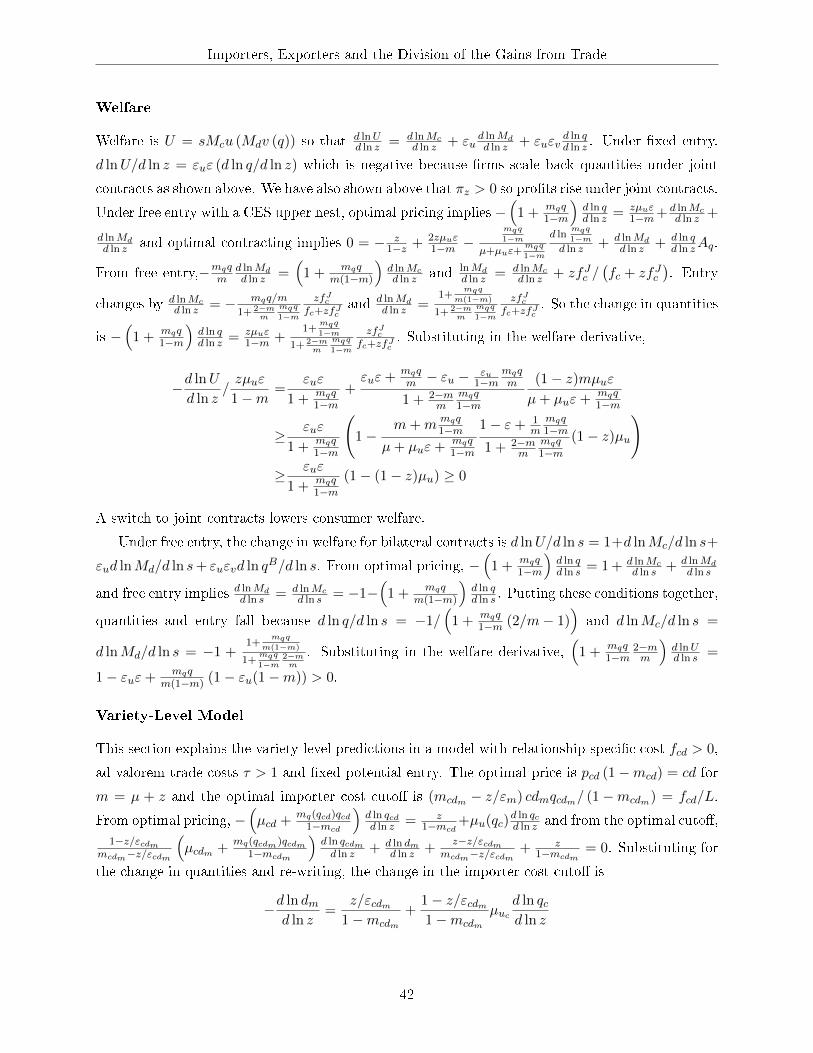
Importers, Exporters and the Division of the Gains from Trade
Welfare
Welfare is U = sMcu (Mdv (q)) so that d lnUd ln z = d lnMc
d ln z + εud lnMdd ln z + εuεv
d ln qd ln z . Under �xed entry,
d lnU/d ln z = εuε (d ln q/d ln z) which is negative because �rms scale back quantities under joint
contracts as shown above. We have also shown above that πz > 0 so pro�ts rise under joint contracts.
Under free entry with a CES upper nest, optimal pricing implies −(
1 +mqq1−m
)d ln qd ln z = zµuε
1−m+ d lnMcd ln z +
d lnMdd ln z and optimal contracting implies 0 = − z
1−z + 2zµuε1−m −
mqq
1−mµ+µuε+
mqq
1−m
d lnmqq
1−md ln z + d lnMd
d ln z + d ln qd ln zAq.
From free entry,−mqqm
d lnMdd ln z =
(1 +
mqqm(1−m)
)d lnMcd ln z and lnMd
d ln z = d lnMcd ln z + zfJc /
(fc + zfJc
). Entry
changes by d lnMcd ln z = − mqq/m
1+ 2−mm
mqq
1−m
zfJcfc+zfJc
and d lnMdd ln z =
1+mqq
m(1−m)
1+ 2−mm
mqq
1−m
zfJcfc+zfJc
. So the change in quantities
is −(
1 +mqq1−m
)d ln qd ln z = zµuε
1−m +1+
mqq
1−m1+ 2−m
m
mqq
1−m
zfJcfc+zfJc
. Substituting in the welfare derivative,
−d lnU
d ln z/zµuε
1−m=
εuε
1 +mqq1−m
+εuε+
mqqm − εu − εu
1−mmqqm
1 + 2−mm
mqq1−m
(1− z)mµuεµ+ µuε+
mqq1−m
≥ εuε
1 +mqq1−m
(1−
m+mmqq1−m
µ+ µuε+mqq1−m
1− ε+ 1m
mqq1−m
1 + 2−mm
mqq1−m
(1− z)µu
)≥ εuε
1 +mqq1−m
(1− (1− z)µu) ≥ 0
A switch to joint contracts lowers consumer welfare.
Under free entry, the change in welfare for bilateral contracts is d lnU/d ln s = 1+d lnMc/d ln s+
εud lnMd/d ln s+ εuεvd ln qB/d ln s. From optimal pricing, −(
1 +mqq1−m
)d ln qd ln s = 1 + d lnMc
d ln s + d lnMdd ln s
and free entry implies d lnMdd ln s = d lnMc
d ln s = −1−(
1 +mqq
m(1−m)
)d ln qd ln s . Putting these conditions together,
quantities and entry fall because d ln q/d ln s = −1/(
1 +mqq1−m (2/m− 1)
)and d lnMc/d ln s =
d lnMd/d ln s = −1 +1+
mqq
m(1−m)
1+mqq
1−m2−mm
. Substituting in the welfare derivative,(
1 +mqq1−m
2−mm
)d lnUd ln s =
1− εuε+mqq
m(1−m) (1− εu(1−m)) > 0.
Variety-Level Model
This section explains the variety-level predictions in a model with relationship-speci�c cost fcd > 0,
ad valorem trade costs τ > 1 and �xed potential entry. The optimal price is pcd (1−mcd) = cd for
m = µ + z and the optimal importer cost cuto� is (mcdm − z/εm) cdmqcdm/ (1−mcdm) = fcd/L.
From optimal pricing, −(µcd +
mq(qcd)qcd1−mcd
)d ln qcdd ln z = z
1−mcd+µu(qc)d ln qcd ln z and from the optimal cuto�,
1−z/εcdmmcdm−z/εcdm
(µcdm +
mq(qcdm )qcdm1−mcdm
)d ln qcdmd ln z + d ln dm
d ln z +z−z/εcdm
mcdm−z/εcdm+ z
1−mcdm= 0. Substituting for
the change in quantities and re-writing, the change in the importer cost cuto� is
−d ln dmd ln z
=z/εcdm
1−mcdm
+1− z/εcdm1−mcdm
µucd ln qcd ln z
42

Importers, Exporters and the Division of the Gains from Trade
As qc =´ dm
0 v(q)dG, total quantity changes by
(qcµuc
+vcdmdm(1−z/εcdm )mcdm−z/εcdm
+´ v′(qcd)qcddGd
µcd+mq(qcd)qcd
1−mcd
)µu
d ln qcd ln z =
−
(vcdmdm
z/εcdm1−mcdm
+´ v′(qcd)qcddGd
µcd+mq(qcd)qcd
1−mcd
z1−mcd
). So d ln qc/d ln z < 0 and total quantities always fall
after joint contracts. Substituting for the change in total quantity, the change in the importer cost
cuto� is (1−mcdm) d ln dmd ln z = −ε−1
cdm
´v′(qcd)qcd
1+ z
µcd+mq(qcd)qcd
1−mcd
1−µcd−εcdm1−µcd−z
dGdqc/µuc+vcdmdm
1−z/εcdm1−mcdm
+´ v′(qcd)qcddGdµcd+
mq(qcd)qcd1−mcd
. We will show that
(1− µcd − µuc ε̄vc)µcd + (1− µcd − εcdm)µuc ε̄vc + mq(qcd)qcd > 0 so that the importer cost cuto�
falls under joint contracts.
First note that the LHS of the inequality is decreasing in µuc ε̄vc under (1 − ε)′ > 0. And
we will need to show that µuc ε̄vc <(1−µcd)µcd
2µcd+εcdm−1 . The RHS of this inequality is decreasing in µcd
because ∂ lnRHS∂µ = − εm+1
(1−µ)(2µ+εm−1) + 1µ < −
εm+12µ+εm−1 + 1
µ = −(1−εm)(1−µ)µ(2µ+εm−1) < 0. So the most binding
inequality is at the highest µcd and εcdm . At these values, the RHS is b(1−b)2−3b . By assumption,
µuc ε̄v < minµv min (1− µv) ≤ b2 which is less than the RHS because 3b2− 3b+ 1 > 0 for b ∈ (0, 1).
So d ln dm/d ln z < 0 and the importer cuto� is lower for joint contracts. Finally, the price change
is d ln pcd/d ln z = −d ln(1 − mcd)/d ln z which gives (1−mcd) d ln pcd/d ln z = mqqd ln qd ln z + z =
− mqq
µ+mqq
1−m
(µu
d ln qcd ln z
)+ µz
µ+mqq
1−m> 0.
Having discussed the changes in observable outcomes across contracts, we will provide conditions
for an increase in the cost cuto� for joint contracts after a reduction in import tari�s. We look
at a reduction in ad valorem tari�s. If τT is the amount paid to exporters, then they receive
just T . The exporter's problem can be written as Πc = τ−1β´ dm
0 [(pcd − cd) qcdLd − fcd] dGd +
τ−1βλcLd
[zqc −
´ dm0 ν(qcd)dGd
]− z2fJc for a continuous choice of contracting denoted by z. Then
the �nal markup is m ≡ µvcd + µuc ε̄vc/z ≡ µv + y/z. Firms will become more likely to enter
into joint contracts if β−1 d2Πcdτ−1dz
=d´ dm0 [(pcd−cd)qcdLd−fcd]
dz − (1− η) d lnQd ln τ−1
d´ dm0 pq
dz > 0. We know
that the �rst terms is positive for joint contracts that are viable. When revenues fall under joint
contracts, as happens in our empirical work, we need to show that aggregate quantities rise with
trade liberalization. Whenever aggregate trade volumes rise with trade liberalization, pro�ts will
be supermodular in contracting choice and the exporter cost cuto� will rise. We therefore provide
conditions on primitives that ensure aggregate trade volumes rise after trade liberalization.
By de�nition, d ln yd ln τ = µ′uqc
µud ln qcd ln τ +
´ v′q(1−µ−ε̄)´v′qdGd
d ln qd ln τ dGd + (εm−ε̄)vmdm´
v′qdGdd ln dmd ln τ . From optimal pric-
ing, −(µ+ µ′q
1−m
)d ln qd ln τ = (1− η) d lnQ
d ln τ −y/z
1−md ln zd ln τ + y/z
1−md ln yd ln τ +µu
d ln qcd ln τ . From optimal contracting,
ln y + (η − 1) lnQ+ lnu′ + ln qc − 2 ln z = ln τ + ln 2fJc /βL so that 2 d ln zd ln τ = d ln y
d ln τ − (1− η)d lnQd ln τ +
(1−µu)d ln qcd ln τ −1. From the optimal cuto� and substituting for optimal prices, d ln dm
d ln τ = − 11−mm (1−
η)d lnQd ln τ −
y/zεm1−mm
d ln yd ln τ + y/zεm−1
1−mm µud ln qcd ln τ . From ln qc = ln
´ dm0 v(q)dGd, the change in total quantities
is d ln qcd ln τ = vmdm´
vdGd
d ln dmd ln τ +
´ v′q´vdGd
d ln qd ln τ . Substituting for the changes in optimal contracts, cuto�s
and markups, we obtain the change in qc in terms of changes in the aggregate quantity Q which can
43

Importers, Exporters and the Division of the Gains from Trade
Figure 3: Distribution of Unit Values and Quality-adjusted Unit Values
-50
510
15Q
ualit
y A
djus
ted
Uni
t Pric
es
-5 0 5 10 15Original Unit Prices
-4-2
02
4C
hang
es o
f Qua
lity
Adj
uste
d U
nit P
rices
-10 -5 0 5 10Changes of Original Unit Prices
Note: Estimates based on the method of Khandelwal et al. (2013).
then be solved using the de�nition of Q ≡´u(qc)dGc. The change in the production cost cuto� is
d ln cmd ln τ
´ dm0 cdqcddGd = −
´ dm0 [(pcd − cd) qcd − fcd/L] dGd− (1− η) d lnQ
d ln τ
´ dm0 pcdqcddGd. The change
in exporter-level quantity is
[1 + µu
vmdm´vdGd
1−y/zεm1−mm + µu
´ v′q´vdGd
dGd
µ+ µ′q1−m
(1 + 1
2 (1/µu − 1) y/z1−m
)+Ac
]d ln qcd ln τ =
−A/2−AQ (1− η) d lnQd ln τ where
Ay ≡(
vmdm´vdGd
y/zεm1−mm + 1
2
´ v′q´vdGd
1
µ+ µ′q1−m
y/z1−mdGd
)/
(1 +´ v′q(1−µ−ε̄)(
µ+ µ′q1−m
) ´v′qdGd
y/z1−mdGd + (εm−ε̄)vmdm´
v′qdGd
y/zεm1−mm
),
A ≡´ v′q´
vdGd
1
µ+ µ′q1−m
y/z1−mdGd +Ay
´ v′q(1−µ−ε̄)(µ+ µ′q
1−m
) ´v′q
y/z1−mdGd,
Ac ≡ Ay
(µ′uqcµu−´ v′q(1−µ−ε̄)(
µ+ µ′q1−m
) ´v′qdGd
(µu − 1
2y/z
1−m(1− µu))dGd − (εm−ε̄)vmdm´
v′q1−y/zεm1−mm µu
)and
AQ ≡ vmdm´vdGd
11−mm+
´ v′q´vdGd
1
µ+ µ′q1−m
(1 + 1
2y/z
1−m
)dGd+Ay
(v′q(1−µ−ε̄)(
µ+ µ′q1−m
) ´v′qdGd
(1 + 1
2y/z
1−m
)dGd + (εm−ε̄)vmdm
(1−mm)´v′qdGd
).
Then aggregate quantity rises after a reduction in tari�s as long as A > 0 and Ac > −1 for z ∈ [0, 1].
Estimating quality
Table 9 shows the quality estimation procedure. Column (1) contains the Broda-Weinstein-Soderbery
estimates and Column (2) contains the �exible method estimates. The elasticities of substitution
are available at the HS 8-digit, and we take the mean for each HS 6-digit category in our data. We
report estimates for the elasticities from the hybrid method of Soderbery. Results are similar with
other elasticity estimates.
The correlation between the unit prices and the quality-adjusted units prices is about 0.8. This
is shown in Figures 3 and 4 which show graph the scatter plots for the prices and the quality-
adjusted prices for each method, and the changes in these variable which are used in the subsequent
estimation.
44

Importers, Exporters and the Division of the Gains from Trade
Table 9: Demand results: Quality Estimation
Dependent Variable: ∆ ln Import Pricecdsht(1) (2)
Coef. Coef.
Variable (S.E.) (S.E.)
ln Import Quantitycdsht/Elasticityh -0.377***
(0.002)
ln Import Quantitycdsht -0.297***
(0.003)
(ln Import Quantitycdsht)2
0.009***
(0.001)
(ln Import Quantitycdsht)2
-0.0003***
(0.00003)
Exporter-Product-Year FE αcsht yes yes
Country-Year FE αst yes yes
N 1,272,789 1,701,645
R2 0.988 0.988
Note: Note: ∆ ln Import Pricecdsht is the change in import prices in logs from period t− 1to t and ln Import Quantitycdsht is the change in import quantities. Elasticityh is theBroda-Weinstein-Soderbery elasticity of substitution for product h. Signi�cance levels areindicated by ∗∗∗, ∗∗, and ∗ for 1, 5 and 10 percent respectively.
Figure 4: Distribution of Unit Values and Quality-adjusted Unit Values: Flexible Approach
-10
-50
510
15Q
ualit
y A
djus
ted
Uni
t Pric
es
-5 0 5 10 15Original Unit Prices
-50
5C
hang
es o
f Qua
lity
Adj
uste
d U
nit P
rices
-10 -5 0 5 10Changes of Original Unit Prices
Note: Estimates based on the �exible method of Section 4.
45