WORKING PAPER SERIES

Implied Volatility from Options on Gold Futures: Do Econometric Forecasts Add Value or Simply Paint the Lilly?

Christopher J. Neely

Working Paper 2003-018C http://research.stlouisfed.org/wp/2003/2003-018.pdf

July 2003 Revised June 2004

FEDERAL RESERVE BANK OF ST. LOUIS Research Division 411 Locust Street

St. Louis, MO 63102

______________________________________________________________________________________

The views expressed are those of the individual authors and do not necessarily reflect official positions of the Federal Reserve Bank of St. Louis, the Federal Reserve System, or the Board of Governors.

Federal Reserve Bank of St. Louis Working Papers are preliminary materials circulated to stimulate discussion and critical comment. References in publications to Federal Reserve Bank of St. Louis Working Papers (other than an acknowledgment that the writer has had access to unpublished material) should be cleared with the author or authors.

Photo courtesy of The Gateway Arch, St. Louis, MO. www.gatewayarch.com

Implied Volatility from Options on Gold Futures: Do Econometric Forecasts Add Value or Simply Paint the Lilly?

Christopher J. Neely*

June 2, 2004

To be possess’d with double pomp, To guard a title that was rich before, To gild refined gold, to paint the lilly,

To throw perfume on the violet, To smooth the ice, or add another hue, Unto the Rainbow, or with taper light

To seek the beauteous eye of heaven to garnish, Is wasteful and ridiculous excess.

— William Shakespeare, King John.

Abstract: Consistent with findings in other markets, implied volatility is a biased predictor of the realized volatility of gold futures. No existing explanation—including a price of volatility risk—can completely explain the bias, but much of this apparent bias can be explained by persistence and estimation error in implied volatility. Statistical criteria reject the hypothesis that implied volatility is informationally efficient with respect to econometric forecasts. But delta hedging exercises indicate that such econometric forecasts have no incremental economic value. Thus, statistical measures of bias and information efficiency are misleading measures of the information content of option prices. Keywords: gold, futures, option, implied volatility, GARCH, long-memory, ARIMA, high frequency JEL subject numbers: F31, G15 * Research Officer, Research Department Federal Reserve Bank of St. Louis P.O. Box 442 St. Louis, MO 63166 (314) 444-8568, (314) 444-8731 (fax) neely@stls.frb.org

Charles Hokayem, John Zhu and Joshua Ulrich provided research assistance. The views expressed are those of the author and do not necessarily reflect official positions of the Federal Reserve Bank of St. Louis or the Federal Reserve System. Any errors are my own.

Implied Volatility from Options on Gold Futures: Do Econometric forecasts Add Value or Simply Paint the Lilly?

Abstract: Consistent with findings in other markets, implied volatility is a biased predictor of the realized volatility of gold futures. No existing explanation—including a price of volatility risk—can completely explain the bias, but much of this apparent bias can be explained by persistence and estimation error in implied volatility. Statistical criteria reject the hypothesis that implied volatility is informationally efficient with respect to econometric forecasts. But delta hedging exercises indicate that such econometric forecasts have no incremental economic value. Thus, statistical measures of bias and information efficiency are misleading measures of the information content of option prices.

Gold has captured the imagination for thousands of years. Yet, despite the growing

importance of derivatives, relatively little research has been done on the gold options market.

Beckers (1984), Ball, Torous and Tschoegl (1985), and Followill and Helms (1990) studied

whether gold options prices obeyed boundary and parity conditions using relatively short

samples of prices from European Options Exchange and/or COMEX. Cai, Cheung and Wong

(2001) looked at the intraday reactions of gold prices to news. But there has been little research

on the information content of gold options prices, although Szakmary, Ors, Kim and Davidson

(2003) include gold in a broad study of the information content of many commodities.1 This

paper seeks to fill this gap in the literature with a comprehensive study of implied volatility (IV)

from options on gold futures from the COMEX division of the New York Mercantile Exchange.

Option prices depend on the expected volatility of the underlying asset return. Latane

and Rendleman (1976) showed that an options pricing model can be inverted to provide the

volatility of the underlying asset until expiry, called implied volatility (IV). Later papers showed

that under risk-neutral pricing, IV should be approximately the conditional expectation of the

realized volatility (RV) until expiry of the underlying asset. Although IV is not a traded asset,

researchers use this relation to motivate the study of IV with a very loose appeal to the efficient

markets hypothesis (EMH): If IV were not an unbiased and informationally efficient forecast of

realized volatility, one could generate excess returns by hedging or trading with better forecasts.

With this motivation, many authors have investigated the predictive properties of IV in a

variety of markets. Most such research has concluded that IV is a good but biased forecast of

realized volatility (RV) until expiry in those markets in which option writer can hedge easily,

like the COMEX market for options on gold futures. Evidence on informational efficiency has

1 Davidson, Kim, Ors and Szakmary (2001) study the proper time scale for options on the same assets.

1

been mixed. The consistent finding that IV is a biased forecast of RV has proved puzzling.

Of course, tests of the properties of IV are implicitly joint tests of market efficiency and

the testing procedures. IV’s apparent bias and informational inefficiency have prompted much

research on the properties of option pricing models and the econometric techniques. This paper

extends that research by applying recent advances in volatility/options research to examine why

IV is biased in gold markets and whether its bias and informational inefficiency matters

economically. Heston’s (1993) stochastic volatility (SV) options pricing model provides the

expectation of RV. High-frequency price data precisely characterize volatility. More

sophisticated econometric models test the informational efficiency of IV.

None of the hypotheses considered for the bias of IV is a plausible explanation.

Specifically, errors-in-variables, sample selection bias, poor properties of the test statistics and a

price of volatility risk model fail to explain the bias and informational inefficiency of IV. But

simulations show that persistence in the IV process might plausibly generate much of the bias.

One set of tests—horizon-by-horizon tests of informational efficiency—often fail to

reject the null, as suggested by Christensen and Prabhala (1998). This paper argues, however,

that such failures do not indicate that horizon-by-horizon tests have better small sample

properties. Instead, horizon-by-horizon tests lack power to reject any hypothesis of interest.

More fundamentally, delta hedging exercises supplement the statistical criteria to assess

the economic value of alternative volatility forecasts. Econometric forecasts do not improve

delta hedging performance, despite the fact that IV fails to subsume those forecasts by statistical

criteria. The contradictory inference from statistical and economic criteria underscores the

importance of assessing the information content of IV with the more relevant measure.

2

2. Option prices and realized volatility

Implicit variance from the Black-Scholes formula

The Black-Scholes (1972) option pricing formula, which counterfactually assumes constant

volatility, underlies almost all research on the forecasting properties of IV.2 Hull and White

(1987) provide the justification for using a constant-volatility model to predict SV: If volatility

evolves independently of the underlying asset price and no priced risk is associated with the

option, the correct price of a European option equals the expectation of the Black-Scholes (BS)

formula, evaluating the variance argument at average variance until expiry:

(1) ( ) ( ) [ ]tTtBST

t tBS

tt VVCEVdVhVCtVSC |)(|)(,, ,2 == ∫ σ ,

where the average volatility until expiry is denoted as: ∫−=

T

tTt dVtT

V ττ1

, .3

Bates (1996) approximates the relation between the BS IV and expected variance until expiry

with a Taylor series expansion of the BS price for an at-the-money option (see Appendix A):

(2) ( )

( ) Ttt

Ttt

TtBS VE

VE

VVar,

2

2,

,2

811ˆ

⎟⎟

⎠

⎞

⎜⎜

⎝

⎛−≈σ .

That is, the BS IV ( ) understates the expected variance of the asset until expiry (2BSσ Ttt VE , ).

This bias is very small, however. Note that (2) depends on (1), which assumes that volatility risk

is unpriced; BS IV is more properly called risk-neutral IV.

Equation (2) implies that the BS IV approximates the conditional expectation of RV ( TtV , ).

This implies that BS IV is an unbiased estimator of RV, that α, β1 = 0, 1 in the following:

2 Garcia, Ghysels, and Renault (2003) survey recent options pricing models. Whaley (2003) looks at the wider derivatives literature. 3 Romano and Touzi (1997) extend the Hull and White (1987) result to include models that permit arbitrary correlation between returns and volatility, like the Heston (1993) model. Because returns and volatility on gold futures have very low correlation, the Romano and Touzi (1997) adjusted

3

(3) , tTtIVTtRV εσβασ ++= 2,,1

2,,

where is RV from t to T and is IV at t for an option expiring at T.2,, TtRVσ 2

,, TtIVσ 4

The second hypothesis is also motivated by (2). If IV is the conditional expectation of RV,

then IV is an informationally efficient forecast of RV. Researchers often investigate this with the

following encompassing regression:

(4) , tTtFVTtIVTtRV εσβσβασ +++= 2,,2

2,,1

2,,

where is RV from t to the expiration of the option at T, is the IV from t to T, and

is some alternative forecast of variance from t to T.

2,, TtRVσ 2

,, TtIVσ

2,, TtFVσ The coefficient estimates ( , )

measure the incremental forecasting value of the IV and econometric forecast. A non-zero

estimate of β

1β 2β

2 rejects the null that IV is informationally efficient with respect to that forecast.

The Properties of implicit volatility

Researchers estimating versions of (3) have found that α is positive and is less than one

for many asset classes and sample periods (Canina and Figlewski (1993), Lamoureux and

Lastrapes (1993), Jorion (1995), Fleming (1998), Christensen and Prabhala (1998), Szakmary,

Ors, Kim, and Davidson (2003), Neely (2004)). That is, IV is a biased and overly volatile

predictor of RV: A given change in IV is associated with a larger change in the RV.

1β

Tests of informational efficiency (4) provide more mixed results. Kroner, Kneafsey, and

Claessens (1993) concluded that combining time series information with IV could produce better

forecasts than either technique singly. Blair, Poon, and Taylor (2001) discover that historical

formula is extremely close to the BS formula for the relatively short-term options in this paper. 4 Estimating (3) with the standard deviation of asset returns and the implicit standard deviation (ISD), rather than variances, provides similar inference to regressions done with variances. While previous versions of this paper used ISDs, the current version uses variances for consistency with the price of variance risk model in Chernov (2002).

4

volatility provides no incremental information to forecasts from VIX IVs. Li (2002) and

Martens and Zein (2002) find that intraday data and long-memory models can improve on IV

forecasts of RV in currency markets. Szakmary, Ors, Kim, and Davidson (2003) find that IV in

gold markets is efficient with respect to historical volatility and a GARCH forecast. Finally,

Neely (2004) finds that IV is not efficient by statistical criteria in foreign exchange markets.

Several hypotheses have been put forward to explain the conditional bias: errors in IV

estimation, sample selection bias, estimation with overlapping observations, and poor

measurement of RV. Perhaps the most popular solution is that volatility risk is priced. This

theory requires some explanation.

The Price of volatility risk

To illustrate the volatility risk problem, consider that there are two sources of uncertainty

about the value of an option in a SV environment: the change in the price of the underlying asset

and the change in its volatility. An option writer must take a position both in the underlying

asset (delta hedging) and in another option (vega hedging) to hedge both sources of risk. If the

investor only hedges with the underlying asset—not vega hedging—then the portfolio return

depends on volatility changes. If volatility fluctuations represent a systematic risk, then

investors must be compensated for exposure to them. In this case, the Hull-White result (1) does

not apply and the BS IV is not even approximately the expected objective variance as in (2).

The idea that volatility risk might be priced has been discussed for some time: Hull and

White (1987) and Heston (1993) consider it. Lamoureux and Lastrapes (1993) argued that a

price of volatility risk was likely to be responsible for the bias in IV from options on stocks. The

volatility risk premium argument rests on the facts that volatility is stochastic, options prices

depend on volatility, and risk premia are ubiquitous in financial markets. If customers desire a

5

net long position in options for business hedging and option writers hedge their exposure to

volatility by buying other options, some agent must still hold a net short position in options and

they will be exposed to volatility risk. IV’s bias could be due to volatility risk.

On the other hand, there seems little reason to think that volatility risk itself should be

priced. While the volatility of the market portfolio is a priced factor in the intertemporal CAPM

(Merton (1973), Campbell (1993)), it is more difficult to see why volatility risk in commodity

markets should be priced. One must appeal to limits-of-arbitrage arguments (Shleifer and

Vishny (1997)) to justify a non-zero price of gold futures volatility risk.

Traditionally, empirical work has assumed that volatility risk could be hedged or is not

priced. But recent research has reconsidered the role of volatility risk in options and equity

markets (Poteshman (2000), Bates (2003), Benzoni (2002), Chernov (2002), Pan (2002),

Bollerslev and Zhou (2003), Ang, Hodrick, Xing and Zhang (2003) and Neely (2004)).

Poteshman (2000), for example, directly estimated the price of risk function from SPX options

data and then constructed a measure of IV until expiry from the estimated volatility process.

Benzoni (2002) finds evidence that S&P 500 variance risk is priced in its option market. Using

different methods, Chernov (2002) also marshals evidence to support this price of volatility risk

thesis for equity and foreign exchange. This paper extends this research by examining whether a

non-zero price of volatility risk can explain the bias in IV for futures on gold.

3. The Data

This paper uses four kinds of data to investigate whether IVs from gold options prices are

biased and informationally efficient: daily settlement prices on gold futures, daily options on

gold futures, high-frequency (30-minute) returns on spot gold prices and daily U.S. interest rates

from the Bank for International Settlements. The high frequency data begin on January 2, 1987,

6

and end on December 31, 1998.5 The COMEX division of the New York Mercantile Exchange

provided daily data on gold futures contracts and options on those contracts. These futures

contracts expire in February, April, June, August, October and December. The options contracts

expire on the second Friday of the month before the futures contract delivery month.

To construct a series of the most liquid contracts, the contract data are spliced in the usual

way at the beginning of each option expiration month. That is, on each trading day of January

and February, the settlement price—collected at 2:00 p.m. central time—and daily range (high

minus low price) for the April futures contract are collected. In addition, the strikes and

settlement prices for the two nearest-the-money puts and two nearest-the-money calls on the

April futures contract are also collected. The options on the April futures contract expire in

March. For each trading day in March and April, data are collected on June futures contracts and

options on those June contracts that expire in May. This procedure collects data on six contracts

each year with five to 53 business days to option expiry.

The usual daily volatility measure extracted from futures prices is as follows:

(5) 2

2

1

2, ln t

t

ttRV r

FF

=⎟⎟⎠

⎞⎜⎜⎝

⎛⎟⎟⎠

⎞⎜⎜⎝

⎛=

−

σ ,

where Ft is the appropriate futures contract settlement price on date t and rt2 is the squared log

return on date t. The annualized futures measure of RV until expiry is the annualized mean

square of the daily returns:

(6) ∑=

++−=

T

iitTtRV r

tT 1

22,, 1

251σ .

5 As a check on robustness, some exercises have been redone with options data that begin on October 4, 1982 and end on July 31, 2002. Intraday price data are not available over the extended period, so results are shown for a period in which comparable data are available.

7

Olsen and Associates provided the high-frequency returns on the spot gold prices. The

daily measure of volatility is the sum of the 48 squared 30-minute returns over each day, from

2:00 p.m. central time to 2:00 p.m. central time, (Anderson and Bollerslev (1998)).6 The

intraday (high frequency) volatility measure for day t can be written as:

(7) . ∑=

=48

1

2,

2,

ititRV rσ

The high-frequency variance measure until expiry is constructed in the same way as the daily

measure in (6). Andersen and Bollerslev (1998) argue that such high-frequency measures more

closely approximate the unobserved volatility process than does the standard deviation of daily

returns. Poteshman (2000), for example, shows that such a high frequency measure eliminates ½

the bias in the predictions of S&P 500 (SPX) index options.

One might consider intraday volatility estimates as a complement to daily volatility,

rather than a substitute. Whether one is interested in the forecasting performance of IV with

respect to intraday or daily volatility data might depend on the application.

4. Econometric methodology

Constructing implied variance

The Heston (1993) SV pricing model provides the benchmark measure of IV, under the

assumption that volatility risk is unpriced. The SV model posits that the futures price and

volatility evolve as follows:

(8) SFdVFdtdF ϖµ += ,

(9) ( ) vvvv dVdtVdV ϖσκθ +−= ,

where F is the futures price at t; V is the instantaneous variance of F’s diffusion process, Sdϖ

6 Results with the 5-minute returns were similar.

8

and νϖd are standard Brownian motion with correlation ρ; and vκ , vv κθ / , and vσ are the

adjustment speed, long-run mean, and variation coefficient of the diffusion volatility.

The SV options prices are functions of ρ, vκ , vθ , vσ , as well as asset price (F), strike price

(X), interest rates (i), time to expiry (T-t), and instantaneous variance (V). Sarwar and Krehbiel

(2000) describe how to obtain values for ρ, vκ , vθ , and vσ from the discrete time series process.

Table 1 shows the estimated parameter vector.

Taking ρ, vκ , vθ , vσ , F, X, i, and T-t as given, instantaneous variance (V(t)) is chosen each

day to minimize the sum of the squared percentage differences between the SV model implied

prices and the settlement prices for the two nearest-to-the-money call options and two nearest-to-

the-money put options for the appropriate futures contract.7

(10) ( )( )( )∑=

−=4

1

2,, Pr/Pr)(minargV(t)

,i

titii tVSVTtσ

where Pri,t is the observed settlement premium (price) of the ith option on day t and SVi(*) is the

appropriate call or put formula as a function of the IV and the parameters in (8) and (9).8

Option prices that violated the no-arbitrage conditions on American options prices (C ≥ F –

X and P ≥ X – F) were discarded. In addition, the observation was discarded if there was not at

least one call and one put price. For a few cases, the quasi-maximum likelihood (QML)

estimation failed to converge and a bisecting grid search was used to find IVs instead. The grid

search estimates appeared consistent with IVs found through QML estimation.

7 Using the full sample to estimate ρ, vκ , vθ , and vσ potentially introduces a look-ahead bias into the IVs. One could instead derive all parameters from options prices, each day, but this method is computationally very difficult in many cases and impossible for some. Although Chernov and Ghysels (2000) find that relying only on options data in pricing and hedging the S&P 500 index contract is best, experiments indicate that it is unlikely to make much difference. In practice, the IVs were not very sensitive to the choice of parameters. 8 Bakshi, Cao, and Chen (1997) and Sarwar and Krehbiel (2000) apply versions of the stochastic

9

Poteshman (2000) and Chernov (2002) show that expected variance until expiry can be

calculated by applying Ito’s lemma to and using the variance process (9). ttVeκ

(11) ( ) ( ) ( )( )[ ]111

, −−⎟⎟

⎠

⎞⎜⎜⎝

⎛−+=

−= −−∫ tT

vt

v

v

v

vT

tutTtt

vetT

VduVEtT

VE κ

κκθ

κθ

,

The expected variance until expiry in (11) is the IV used to predict realized variance until expiry.

This procedure eliminates the biases in (2).

Bates (1996) reports that using at-the-money options has become increasingly popular. There

are three reasons for this practice: 1) At-the-money options prices are most sensitive to changes

in IV, meaning that changes in IV should be reflected in those options. 2) At-the-money options

are usually the most liquid. 3) Research has found that IV from at-the-money options provides

the best estimates of future realized volatility (e.g., Beckers (1981)). Despite the fact that

researchers have varied the number of options, the type of options, and the weighting procedure,

it has been common to rely heavily on at-the-money options. Therefore, choosing the two nearest

calls and two nearest puts for estimating IV each day seems to be a reasonable procedure.

Alternative forecasts

Four types of models provide alternative forecasts of RV to test IV’s informational

efficiency: autoregressive integrated moving average (ARIMA) models, long-memory ARIMA

(LM-ARIMA) models, generalized autoregressive conditional heteroskedastic (GARCH)

models, and ordinary least squares (OLS) models with several independent variables.9 The

Bayesian Information Criterion (BIC) chose the specific structure (e.g., the AR and MA orders

of the ARIMA model) of each of the four classes of models during an in-sample period, 1987

volatility (SV) option pricing model to hedging and pricing problems. 9 Poon and Granger (2003) review the literature on forecasting volatility in financial markets. Pong, Shackleton, Taylor, and Xu (2003) compare the forecasting ability of ARFIMA models with IV by

10

through 1991 (Schwarz (1978)). The in-sample structure and in-sample coefficient estimates

were then fixed and used to forecast RV until expiry in the out-of-sample period, 1992-1998.

Appendix B describes these forecasts in detail.

Summary Statistics

Table 2 displays the summary statistics for the annualized one-period volatility of gold

prices and its forecasts in the left-hand panel and the analogous statistics for volatility until

option expiration in the right-hand panel. While the empirical forecasting work will measure

volatility with variance, to be consistent with Chernov’s (2002) price of risk model, the summary

statistics in Table 2 present the more easily interpretable standard deviation measures. The top

panel measures daily volatility with the annualized root of daily sums of log 30-minute squared

changes while the bottom panel uses the annualized root sum of squared changes in daily log

futures prices. All statistics are annualized and in percentage terms.

Mean one-step realized volatility (σtRV ) is 10.44 percent per annum by the high-

frequency measure and 8.40 percent per annum by the daily futures price measure. The mean of

the one-step-ahead forecasts are higher than actual volatility, but the forecast means are based

only on in-sample data, not the whole sample as the statistics in Table 2. The forecasts are, of

course, less variable than the realized volatility. The one-step-ahead forecasts in the left-hand

panel have first-order autocorrelation coefficients (row AC1) that range from 0.26 to 0.98.

Comparing the top panel to the bottom panel shows that the daily high frequency volatility

measure (column labeled σtRV) is also much more highly autocorrelated than the measure

constructed from daily futures prices. The former has first-order autocorrelation of 0.55 to the

mean-squared error and R2 metrics.

11

latter’s figure of 0.11. This is consistent with Andersen and Bollerslev (1998), who argue that

high frequency volatility more precisely measures unobserved volatility than daily volatility.

Figure 1 illustrates the mean-reverting time series behavior of both measures of realized

volatility until the next option expiration (σt,THF and σt,T

Fut ) and IV (σt,T IV). IV appears to track

both realized volatility series reasonably well, as one might expect.

5. Testing for bias and inefficiency using overlapping observations

Is implicit variance an unbiased forecast of realized variance?

If IV is the market’s prediction of RV and expectations are rational, then IV should be an

unbiased estimator of future volatility. That is, α, β1 = 0, 1 in the following model:

(3) , tTtIVTtRV εσβασ ++= 2,,1

2,,

This paper initially follows most previous research in estimating (3) with OLS and telescoping

samples.10 For overlapping horizons, the residuals in (3) will be autocorrelated and, while OLS

estimates are still consistent, the autocorrelation must be dealt with in constructing standard

errors. Such data sets are described as “telescoping” because correlation between adjacent errors

declines linearly and then jumps up at the point at which contracts are spliced. To construct

correct measures of parameter uncertainty, this paper follows Jorion (1995) in using the

following covariance estimator:

(12) , ( ) ( ) 11 'ˆ'ˆ −− Ω=Σ XXXX

where , X is the T by K matrix of (∑∑∑= ==

++=ΩT

s

T

sttsstst

T

tttt XXXXtsIXX

11

2 ''ˆˆ),('ˆˆ εεε )

10 Christensen and Prabhala (1998) also estimate versions of (3)and (4) with feasible generalized least squares (FGLS) for one short subperiod but find it does not help IVs bias or efficiency. See Table 6 in that paper.

12

regressors, Xt is the tth row of X, tε is the residual at time t, and I(s,t) is an indicator variable

that takes the value 1 if the forecast from period s overlaps with the forecast from period t.

Table 3 shows estimates of the coefficients in (3) for gold options-on-futures and realized

volatility in gold market from 1987 to 1998, with robust standard errors as in equation (12).

Consistent with previous research in other markets—e.g., Jorion (1995); Canina and Figlewski

(1993); Lamoureux and Lastrapes (1993); Fleming (1998); Christensen and Prabhala (1998) and

Neely (2004) —the coefficient is always positive, but also much less than the hypothesized

value of one under the null that the IV is unbiased. equals 0.48 and 0.56 for the intraday and

daily futures variance measures, respectively. When is less than one, IV is said to be an

excessively volatile predictor of subsequent realized volatility because a given change in IV is

associated with a smaller change in future realized volatility. The Wald p-values in the sixth

column of Table 3—constructed with robust covariance matrices—strongly reject that α,β

1β

1β

1β

1

equals 0,1. In other words, the bias is statistically significant for both data sets.

High frequency RV is more closely correlated with IV than is daily futures RV. The R2

for the intraday data (top row) is 0.49 while that for the daily futures data is only 0.37. This is

consistent with the idea that high frequency volatility is a less noisy measure of the unobserved

underlying volatility in the market.

Is implied volatility informationally efficient?

If IV is approximately the conditional expectation of RV, as implied by (2), then it

subsumes all publicly available information. To test this proposition, one can forecast volatility

using the econometric models described in Appendix B—ARIMA, LM-ARIMA, GARCH,

OLS—to see if any of these forecasts of volatility over the life of the option add information to

IV. That is, one can regress RV on IV and a forecast of variance:

13

(4) tTtFVTtIVTtRV εσβσβασ +++= 2,,2

2,,1

2,, ,,

and test if β2 is positive.11 If IV subsumes the other forecast of RV, then one should fail to reject

β2 equals zero (Fair and Shiller (1990)).

r the out-of-sample period, 1992 through 1998.

Using o

e

the

evel in three of four

he

that

Table 4 presents the results of OLS estimation of equation (4), with telescoping samples

and robust standard errors (equation (12)), ove

nly out-of-sample data creates a genuinely ex ante exercise with which to test the four

econometric forecasts. From left to right, the four panels of Table 4 display the results from

forecasts with an ARIMA model, a long-memory ARIMA model, a GARCH(1,1) model and th

OLS model. The top row of Table 4 measures volatility with the daily sums of 30-minute

squared returns to while the bottom row uses the daily futures price variance.

With the high-frequency measure of volatility (top row of Table 4), the coefficients on

forecasts ( 2β ) are always positive and statistically significant at the five percent l

cases. Similarly, the bottom row of Table 4 shows that with the futures price as the volatility

measure, the coefficients on the forecasts ( 2β ) are positive and statistically significant for two of t

four forecasts. The coefficients on the LM-ARIMA and OLS forecasts are significant for both the

intraday and daily realized variance data. The positive and statistically significant 2β reject the

hypothesis that IV is informationally efficient. As with the bias regressions in Table 3, the R2s for

the high-frequency regressions (top row of Table 4) are larger than the corresponding R2s for the

futures-volatility regressions (bottom row) in each case. IV is more closely correlated with high-

frequency volatility than with the daily volatility measure.

invariant to orthogonalization of the regressors.

11 It is not necessary to make the econometric forecast orthogonal to IV before using it in (4). The t statistic on provides the same inference (asymptotically) as the appropriately constructed F test for the hypothesis that β

2β2 = 0. And the F test—which is based on the R2 of the regression—is

14

6. Why is implicit variance biased and informationally inefficient?

IV for gold futures has been shown to be apparently biased and inefficient. There are two ways

to explain such a result: 1) failure of the EMH; 2) or failure of the testing procedures. Because the

EMH seems theoretically difficult to assail—at least without appeals to information problems—

economists have focused their attention on the testing procedures, including the possibility that a

non-zero price of volatility risk could produce bias and inefficiency.

Problems with the testing procedures fall into several categories: 1) peso/finance minister

problems; 2) measurement error in IV; 3) sample selection bias; 4) use of overlapping samples; or

5) a non-zero price of volatility risk. This section considers whether these issues could plausibly

generate the bias and inefficiency.

called peso or finance-minister problems—might generate

apparently biased predictions of realized volatility. That is, agents might have rationally priced

options while taking into account extreme but low probability events that were not observed in

the sample. Conversely, other low probability events might have been observed too often in the

sample. For example, the market might have rationally priced in a low probability of periods of

extremely volatility that never occurred. If such expectations increased with realized volatility,

IV would appear unconditionally and conditionally biased, producing overly volatile predictions.

It seems unlikely that sample-specific variation is to blame for the bias observed in IV

because IV’s bias is a ubiquitous result across assets and sample periods (Poteshman (2000)).

Further, the only way to correct for such problems is through longer spans of data; the 12-year

data set used here is already very long by the standards of the options literature.

Peso problems

Unusual sampling variation—

15

Measurement error

Measurement error in IV is an obvious candidate explanation for its apparent bias and

ll known that error in the independent variable creates attenuation bias; the

esti

sts

es

sec

wo

statistics of the IVs from the three option

pric 7)

s) each day.

Tab

th

inefficiency. It is we

mated regression coefficient is inconsistent, smaller in absolute value than the true

coefficient. Christensen and Prabhala (1998) illustrate that errors-in-variables could also explain

IV’s failure to subsume other forecasts. Specifically, if both IV and econometric foreca

constitute “noisy” predictions of RV, then an optimal predictor will put some weight on each.

The conventional wisdom, however, is that there is not much error in IV estimation (Bat

(1996)). One source of error is specification error from using the wrong options model. The

ond source is idiosyncratic error from microstructure effects like asynchronous prices and

bid-ask spreads in both the options and the underlying futures. Bates (2000) decomposes the t

types of errors for options on S&P 500 futures contracts and concludes that IV is not very

sensitive to the choice of two-factor pricing models.

The IV used in this paper is also not very sensitive to the choice of (risk-neutral) option

pricing model. Table 5 illustrates the similar summary

ing models: the SV pricing model of Heston (1993), the Barone-Adesi and Whaley (198

early exercise correction to the Black (1976) model, and the Black (1976) model. The IVs from

the three models are extremely highly correlated and have very similar summary statistics. The

results in this paper are robust to the choice of (risk-neutral) option pricing model.

One can measure the error in IV estimation by examining the maximal difference between

the IVs implied by the two closest calls and two closest puts (six possible pairs of IV

le 6 shows that these differences are small. The median difference is about 20 basis points

and the 90 percentile is about 77 basis points.

16

Because these options have slightly different degrees of moneyness, they might imply

different volatility (Hull (2002)). To remove variation caused by different degrees of

mo tions

,

ntile is

ias in S&P

t is, if one cannot observe IV or RV during periods of extreme RV—

per

s.

ight produce very poor small-sample estimates. To investigate the

con

the

neyness, one can examine the absolute difference between IVs from put-call pairs of op

with exactly the same strike price on the same day.12 In the absence of bid-ask spreads

transactions costs, or early exercise, these differences should be exactly zero. Indeed, they are

very small. The median difference, for example, is only 2 basis points and the 90th perce

11 basis points. Experiments conducted in simulations—not reported for brevity—indicate that

error less than 2 percent has almost no effect on the estimates of bias and efficiency.

Sample selection bias

Engle and Rosenberg (2000) suggest that sample selection bias is responsible for b

500 index options. Tha

haps because liquidity dries up because of uncertainty—then there will be sample selection

bias in the regression of RV on IV. Selection bias might result if volatility until expiry were

systematically higher or lower on days with missing IV than on other days. But this is not a

problem in the present data set. IV is available in all periods for which there are futures price

Overlapping samples

Christensen, Hansen, and Prabhala (2001) argue that the usual regressions conducted with

overlapping forecasts m

sequences of such overlapping forecasts one can either simulate the distribution of the test

statistics under the null hypothesis of unbiased forecasts or one can independently estimate

predictive equation (3) for each forecast horizon. The simulation method has the advantage of

12 Experiments suggest that correcting IV estimates for the volatility smile made very little difference in the bias or informational efficiency of IV. Error generated by the volatility smile seems unimportant for the issues of bias and informational efficiency.

17

greater power in pooling all horizons together. The fixed horizon method is computationally sim

and does not require one to assume that the regression has the same coefficient vector at each

horizon. This paper confronts the overlapping observations problem in both ways.

What effects do autocorrelation and errors-in-variables have on the IV coefficient? Ma

and Shapiro (1986) and Stambaugh (1986) argue that autocorrelation and measur

pler

nkiw

ement error in

the

modified logarithmic

tran nd

n to

el with the whole sample, saving the estimated

3. s, construct RV as the annualized sum until expiry of the

able 3. Construct IV as

4.

dependent variable will tend to bias the coefficient toward zero. To investigate these effects,

this paper judges the significance of the parameters by using a plausible data generating process

to simulate the distribution of the parameter estimates under the null, as in Mark (1995), Jorion

(1995), Kilian (1999) and Berkowitz and Giorgianni (2001).

Both GARCH and log-ARIMA models are used to simulate and predict RV and IV until

expiry. The ARIMA model was estimated and simulated on a

sformation of the daily variance data because they are truncated at zero, highly skewed, a

kurtotic. The ARIMA forecasts were then transformed with a Taylor series expansio

produce approximately conditionally unbiased forecasts of RV until expiry. Appendix C

describes these transformations in detail.

The simulation procedure for the GARCH/ARIMA models were as follows:

1. Estimate the GARCH/ARIMA mod

coefficients and residuals.

2. Construct 1000 simulated variance samples by bootstrapping.

For each of the 1000 sample

squared returns. The sample sizes will be the same as those in T

the optimal multiperiod forecast of RV over the appropriate horizon.

Regress simulated RV-until-expiry on simulated IV, saving the test statistics.

18

5. re consistent with

autocor tics in the

real

ows

log

Examine whether the coefficients and test statistics from the real data a

the distribution of the coefficients and test statistics from the simulated data.

The simulated data were checked to ensure that the summary statistics—especially the

relations—of the simulated data were reasonably close to the analogous statis

data and the simulated IV was an approximately unbiased predictor of simulated RV.

Table 7 displays the results of the Monte Carlo experiment simulating the regression of RV

on IV. The upper panel shows the GARCH-t generating process results; the lower panel sh

-ARIMA results. The first four columns summarize the distribution of α ; columns five to

eight show statistics on the distribution of 1β ; and the final four columns display the percentage

of rejections from the simulated Wald statistics and the simulated R2s.

The simulated GARCH model generates considerable bias in the estimates of β1, the 5th

percentiles of the 1β distributions are 0.51 to 0.49. And the Wald statistics reject the null 71 and

50 h d

ra

e

the estimates of β1, but not as much as the

GA

to

ted

percent of the time. The β estimates from the real data—see Table 3—are in t e left-han

tail of the simulated distributions, 97 and 87 percent of the simulated β are greater than those

from the real data for the int day and futures variance measures, respectively. The GARCH

model does not replicate the bias found in IV.

The lower half of Table 7 shows that data produced under the null of unbiasedness from th

log-ARIMA model produces substantial bias in

1

1

RCH model. The 5th percentiles of the 1β distributions are 0.60 to 0.61 for intraday and

daily measures. The median estimates of β are much larger, however, ranging from 0.83

0.89 and the Wald statistics reject 42 and 21 percent of the time. The three of the four simula

R

1

2 distributions appear to be consistent with the R2s from the actual data (see Table 3).

19

Persistent-regressor bias in the GARCH and log-ARIMA data generating processes cannot

explain the whole conditional bias observed in IV. A generating process with greater persistence

in v

ce.

non

t),

k k,1

fewer than 20 observations rate were not estimated, leaving a minimum forecast horizon of

olatility might have produced the apparently biased and informationally inefficient

coefficients that we observe in the data. For example, the fractionally cointegrated relation

between IV and RV found by Bandi and Perron (2003) might produce enough persisten

Is IV Unbiased in Horizon-by-Horizon Estimation? Christensen, Hansen, and Prabhala

(2001) advocate the second method of correcting problems with overlapping samples: Use

overlapping samples—fixed forecast horizons.13 To examine how IV might vary as a

predictor across forecast horizons, one can estimate (3) separately for each horizon (k = T –

(13) tTtIVkkTtRV εσβασ ++= 2,,1,

2,, ,

where α and β denote the coefficients for a horizon of k days until expiry. Cases (horizons)

with

seven business days and a maximum horizon of 50 business days. There were 26 to 71

observations for each forecast horizon. Most horizons had 71 observations.

Figure 2 shows the series of values for kα , 1,ˆ

kβ , and the p-values for the likelihood r

(LR) test that α , β = 0, 1. As in the overlapping horizon results in Ta

atio

k k,1 ble 4, the kα are

positive and the kβ are much less than on k for the futures data (solid line) are usually

nul

1,ˆ ˆ

greater than those for the high-frequency volatility measure (dashed line). The LR tests almost

always reject the l that α

e. The 1,β

k, βk,1 = 0, 1 for both data sets. The mean of the horizon-by-

horizon 1,ˆ

kβ s in Figure 2 are just slightly larger—0.497 and 0.582—than those in the

overlapping results in Table 4. Contrary to results in Christensen and Prabhala (1998) and

13 There is a modest amount of overlap at horizons greater than 50 business days.

20

Christensen, Hansen and Prabhala (2001) horizon-by-horizon does not make IV appea

significantly less biased.

Is IV informationally efficient in fixed horizon tests? Tests of informational efficienc

suffer from potentially poo

r

y also

r properties of overlapping data sets. One can estimate equation (4)

for

ents were fixed by a search over the in-sample

-1991) period and only out-of-sample forecasts (1992-1998) were used to estimate (14).

Aft

ata.

The igure 3

o

he null of

fixed horizons to alleviate such problems.

(14) tTtFVkTtIVkkTtRV εσβσβασ +++= 2,,2,

2,,1,

2,, .

The forecasting model structure and coeffici

(1987

er deleting forecast horizons with fewer than 20 observations, horizons ranged from 8 to 49

business days and had between 23 and 41 observations during the out-of-sample period.

The top row of Figure 3 displays the series of coefficients from maximum likelihood

estimation of the pooled model described by (14) on high-frequency (intraday) volatility d

2,ˆ

kβ coefficients are very volatile but positive at most horizons. The bottom row of F

shows the corresponding LR test p-values for the hypothesis that the βk,2 coefficients are equal t

zero. The LR p-values are sometimes less than 0.05—rejecting the null of informational

efficiency—for horizons less than 30 business days. The forecasts have a fair proportion of

rejections at these short horizons. The frequency with which the tests reject the null does not

seem to clearly answer the question as to whether IV is informationally efficient for high-

frequency volatility. However, with such a small sample size and correspondingly low power,

one might expect low power to reject the null from such a test. Therefore obtaining rejections in

one quarter of the cases casts some doubt on the null of informational efficiency.

Figure 4 shows the corresponding statistics using daily futures prices to measure

volatility. The 2,ˆ

kβ coefficients are extremely volatile and only sometimes reject t

21

in ational efficiency. Again, this is probably due to the paucity of observations invol

estimating the m els and the difficulty of fitting forecasting models to the highly skewed an

kurtotic squared daily return series. The failure to reject informational efficiency with horizon-

by-horizon tests probably reflects low power rather than better small sample properties.

A Non-zero price of volatility risk

Risk-neutral valuation requires that the risks associated with a position in an option

form ved in

od d

either

. This is not necessarily the case. And it is only under risk-

neutral

s, one estimates

the

can be hedged or are not systematic

valuation that IV is approximately the conditional expectation of RV (2). Recent

research has considered the possibility that volatility risk is responsible for the bias found in BS

IVs (e.g., Poteshman (2000), Benzoni (2002), Chernov (2002), Neely (2004)).

Chernov (2002) derives an expression for expected realized variance until expiry in terms of

the implied risk-neutral expected variance until expiry (see Appendix D). That i

following prediction equation to see if the coefficient, β1, is equal to one:

(15) ( ) ( ) ttMv

Mv

Qv

QvTtTtIV

Mv

Mv

Qv

QvTtTtRV V εκθκθγσβκθκθασ +++= ,,,,,, ,

2,,1,

2,, ,

where the coefficients, αt,T, and γt,T, are functions of time to expiry and the parameters of the

eutral risk-n ( )Qv

Qv κθ , and objective SV processes ( )M

vMv κθ , . If volatility risk is not priced, the

in

f e

cor

There are potentially at least 2 ways to estimate equation (15). The first method is to

risk-neutral and objective SV processes are the same and the coefficient vector αt,T, β1, γt,T

(15) equals 0,1,0. In this case, the conventional prediction equation (3) is appropriate.

Citing equation (15), Chernov (2002) argues that the conventional regression o averag RV

on the risk-neutral IV is misspecified because instantaneous variance—which is heavily

related with the risk-neutral IV—is omitted. This omission biases the coefficient (β1) on risk-

neutral IV downwards.

22

estimate the three hyperparameters ( )1,, βκθ Qv

Qv , conditional on the time to expiry (T–t) and the

parameters from the time series estimation of the process— ( )MM θκ , in (15)—to help construct

the imate coefficients. This imposes the model’s restrictions across horizons, requires one to est

only 3 free parameters, then test whether the data reject that βk,1 is equal to one.

(16) ( ) ( ) tkTtQQQ

kTtR VTtT ,,1,2

,,1,2

,, ,, εθδσβθκασ +++−=

This method is potentially powerful, getting precise estimates, but imposes restrictions on the

functional form—ruling out jumps in volatility, for example.

QkTtIVk t ,,κ−

he second method of estimating the price-of-volatility-risk model is to estim te the

st

IV is unbiased after the inclusion

of t

ssors are estimated with error, one

sho

8

ated

onl

T a

parameter vector αt,T, β1, γt,T for each horizon with no cross-horizon restrictions. One can te

whether the data reject the model’s implication that risk-neutral

he volatility risk premium. That is, one tests if β1 = 1.

Either estimation method requires estimates of instantaneous variance as well as risk-neutral

IV. Instantaneous variance is taken to be the daily volatility estimate from intraday data.

Because this measure and—to a lesser extent—the IV regre

uld use instrumental variables to estimate (16) (Chernov (2002)). The BIC selects instruments

from lagged values of the estimated instantaneous variance, IV and forecasts of RV. Table

presents the results of Generalized Method of Moments (GMM) (Hansen (1982)) estimation of

the parameters (16), accounting for the overlapping observations in the standard error (equation

(12)). T-tests clearly reject the null that IV is an unbiased forecaster.

Estimating only three hyperparameters imposes fairly strong restrictions on the model,

however. The price-of-volatility-risk model might do better if αk, βk,1, γk were estimated

separately for each horizon. This is similar to Chernov’s procedure, except that he estim

y one forecast horizon (one-month).

23

Figure 5 shows the results of estimating (16) by GMM with instrumental variables. The

model rejects the null that 1,ˆ

kβ equals one for all but a few horizons. Curiously, one of the few

horizons that fails to reject unbiasedness

is the one-month horizon (20-21 business days), for

whi ting

in (

lts

om

ciency does not tell us

more relevant test of IV’s forecasting

abil

lio is

ch Chernov also failed to reject unbiasedness with equities and foreign exchange. Permit

a price of volatility risk, as 16), does not resolve the puzzle of IV’s bias for gold futures.

To examine the robustness of the results, Figure 5 was reconstructed under alternative

assumptions, including a range-based and moving-average based estimates of instantaneous

variance and OLS estimation of the model. None of the alternative estimation methods—resu

itted for brevity—support the unbiasedness hypothesis.

6. Economic implications of inefficiency: tracking error

Judging the information content of options prices with statistical measures has never been

very tightly motivated. In particular, the frequent rejection of bias and effi

about the economic significance of these shortcomings. A

ity is whether econometric forecasts can usefully augment the IV in delta hedging. To

examine this, one can compare the delta hedging tracking error with two measures of variance:

1) only IV or 2) an ex ante function of IV and variance from econometric forecasts.14

The tracking error from delta hedging a call option on futures is calculated as follows:

1. In the first period of a contract, the agent sells a call option, puts the proceeds into bonds,

and takes a position of ∆(1) units in the futures contract. The value of this portfo

initially zero because the long bond position offsets the short call.

14 Bollen and Whaley (2003) also examine vega hedging for S&P 500 index options. This exercise is not pursued here because the aim is to evaluate the contribution of econometric forecasts to delta hedging. Green and Figlewski (1999) examine the risks inherent in pricing and hedging options and the extent to which using a higher than expected IV can compensate for these risks.

24

(17) ( ) 0 )1,- )1,000 )0()0( ==+= XF

BSXF

BSCB (C(C)( V) ( VV

On subsequent business days, the agent’s bond holdings are augmented by interest on

bond position and gains (losses) on the previous futures position. Th

2. the

e agent also adjusts

tures position to the current delta, ∆(t). The portfolio’s value on day t is the fu

(18) ( ) ( ) ( ) ),1,11 )1( )(365 tC(ttF)(tVe t VV(t) tFtFr n

∆−−∆∆+−⎟⎞⎜⎛ −+−= , XXB⎠⎝

where VB(t-1) is the value of the bonds on t-1, there were n calendar days since the last

business day, ∆F(t) is the change in the value of the futures price from t-1 to t, ∆(t-1) is

utures position at t-1 and ∆C(t) is the change in the call price from t-1 to t.

3.

The ts can

imp

The for (λ) versus the

eco

k is a constant. The

mark model constrains λ = 1 and chooses k to minimize in-sample delta hedging error.

he

the f

On the last day of the contract, the agent closes the futures position. The tracking error is

the difference between the value of bond holdings and the option’s value.

exercise aims to determine whether one-step-ahead ex ante econometric forecas

rove delta hedging over a benchmark model using only the implied instantaneous variance.

ecast-augmented model picks the relative weight of instantaneous volatility

nometric forecast (1-λ) and a constant, from a grid, to construct the instantaneous variance

estimate for the delta function to minimize tracking error in the in-sample period (1987-1991).

The augmented model’s instantaneous variance is given by the following:

(19) ktVtVtV FSVAug +−+= )()1()()( λλ ,

where VSV(t) is the instantaneous variance from the SV model, VF(t) is the one-step-ahead

forecast volatility from one of the four econometric forecasting models and

bench

Both models choose a negative k to make delta larger and more volatile to hedge better at t

daily frequency.

25

To implement the delta hedging experiment, at the beginning of each contract period the c

with the longest time continuously near-the-money was chosen as the call to hedge. When tha

call left the mone

all

t

y, the position was closed out, the tracking error calculated, and a new call

cho

r

est procedure. In all

cas

re

crit .

long-memory models, to examine why IV is an inefficient and biased predictor of the realized

of the explanations previously suggested—imprecise volatility

esti

Horizon-by-horizon estimation usually cannot reject that IV is informationally efficient. One

sen to hedge. All positions were closed at the end of splicing periods.

Table 9 shows the percentage improvement in the out-of-sample tracking error using the fou

econometric forecasts. The tracking error is the sum of the absolute tracking errors for each

option contract followed. Standard errors are calculated with the Newey-W

es, most weight was put on the instantaneous variance and relatively little on the econometric

forecasts; λ’s ranged from 0.4 to 0.9. Six of the eight point estimates are positive but none a

statistically significant. Consistent with the idea that there is more information about variance in

intraday data, weights on the intraday variance forecasts are larger than those from the daily data.

Econometric forecasts do not consistently reduce delta-hedging tracking error. This sheds

new light on rejections of bias and recent rejections of informational efficiency (Li (2002) and

Martens and Zein (2002)). It highlights the need to evaluate forecasts with the most relevant

eria. In the case of options, statistical criteria are simply not as informative as delta hedging

7. Conclusions

This paper has exploited high-frequency data and new econometric techniques, including

volatility of gold futures. None

mation, overlapping samples, sample selection bias, a price of volatility risk, etc.—can

plausibly explain this bias and inefficiency. Persistent regressor bias can explain some of the

bias in overlapping samples.

26

should not conclude, however, that the better small sample properties of horizon-by-horizon

estimation procedures rescue the unbiasedness hypothesis. Rather, the failure to reject almost

certainly reflects a lack of pow

er. There are only 23 to 41 observations per horizon, in this

sam

ce,

al in

e information content of IV. Using econometric forecasts to supplement IV in delta

hed

ple.

While statistical criteria judge IV to be a biased and inefficient predictor of realized varian

implied instantaneous variance is informationally efficient by an economic criterion, delta

hedging tracking error. This underscores the point that choosing the proper criterion is cruci

judging th

ging just gilds the lily.

27

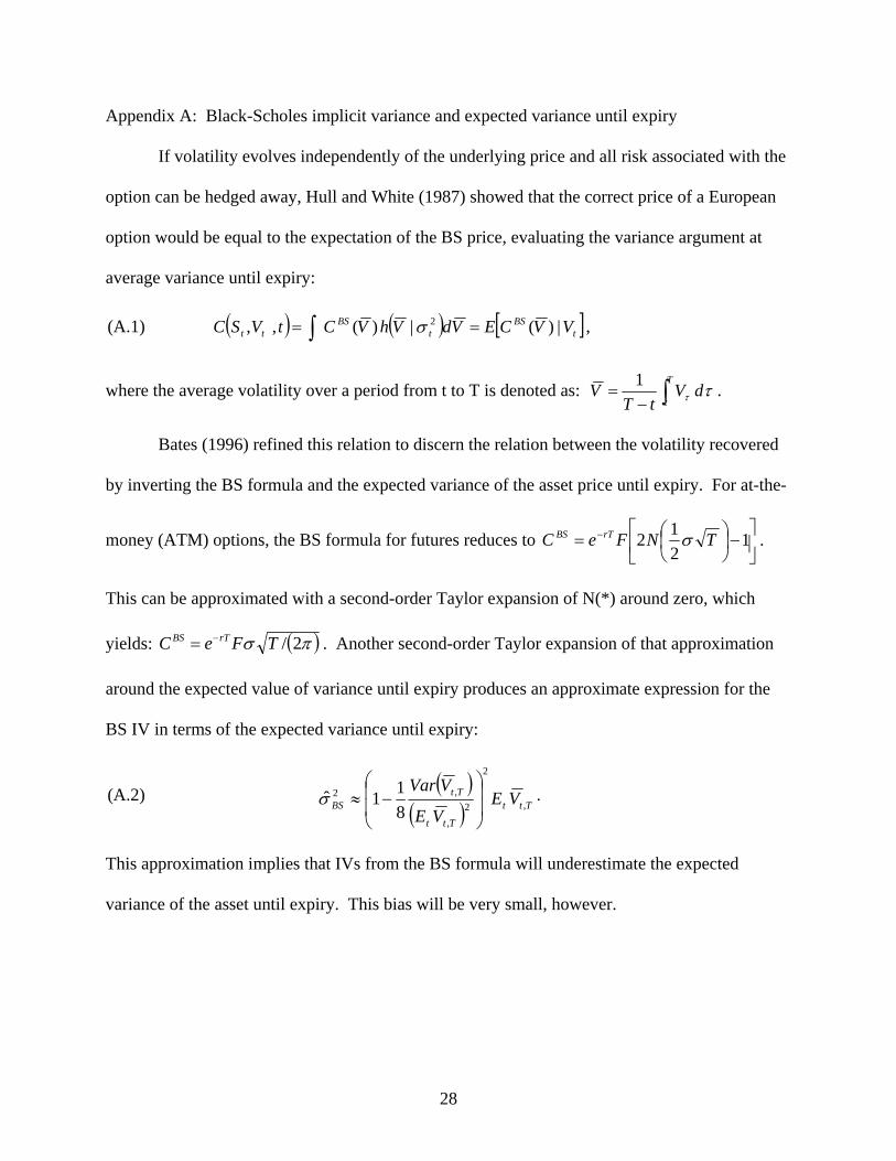
Appendix A: Black-Scholes implicit variance and expected variance until expiry

If volatility evolves independently of the underlying price and all risk associated with the

option can be hedged away, Hull and White (1987) showed that the correct price of a European

option would be equal to the expectation of the BS price, evaluating the variance argument at

average variance until expiry:

(A.1) ( ) ( ) [ ]tBS

tBS

tt VVCEVdVhVCtVSC |)(|)(,, 2 == ∫ σ ,

where the average volatility over a period from t to T is denoted as: ∫−=

T

tdV

tTV ττ

1 .

Bates (1996) refined this relation to discern the relation between the volatility recovered

by inverting the BS formula and the expected variance of the asset price until expiry. For at-the-

money (ATM) options, the BS formula for futures reduces to ⎥⎦

⎤⎢⎣

⎡−⎟

⎠⎞

⎜⎝⎛= − 1

212 TNFeC rTBS σ .

This can be approximated with a second-order Taylor expansion of N(*) around zero, which

yields: ( )πσ 2/TFeC rTBS −= . Another second-order Taylor expansion of that approximation

around the expected value of variance until expiry produces an approximate expression for the

BS IV in terms of the expected variance until expiry:

(A.2) ( )( ) Ttt

Ttt

TtBS VE

VE

VVar,

2

2,

,2

811ˆ

⎟⎟

⎠

⎞

⎜⎜

⎝

⎛−≈σ .

This approximation implies that IVs from the BS formula will underestimate the expected

variance of the asset until expiry. This bias will be very small, however.

28

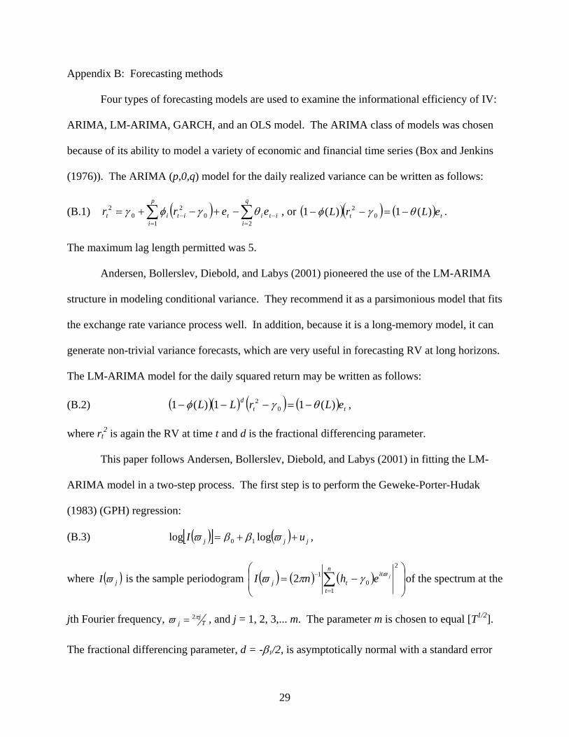
Appendix B: Forecasting methods Four types of forecasting models are used to examine the informational efficiency of IV:

ARIMA, LM-ARIMA, GARCH, and an OLS model. The ARIMA class of models was chosen

because of its ability to model a variety of economic and financial time series (Box and Jenkins

(1976)). The ARIMA (p,0,q) model for the daily realized variance can be written as follows:

(B.1) , or ( ) ∑∑=

−=

− −+−+=q

iitit

p

iitit eerr

210

20

2 θγφγ ( )( ) ( ) tt eLrL )(1)(1 02 θγφ −=−− .

The maximum lag length permitted was 5.

Andersen, Bollerslev, Diebold, and Labys (2001) pioneered the use of the LM-ARIMA

structure in modeling conditional variance. They recommend it as a parsimonious model that fits

the exchange rate variance process well. In addition, because it is a long-memory model, it can

generate non-trivial variance forecasts, which are very useful in forecasting RV at long horizons.

The LM-ARIMA model for the daily squared return may be written as follows:

(B.2) ( )( ) ( ) ( ) ttd eLrLL )(11)(1 0

2 θγφ −=−−− ,

where rt2 is again the RV at time t and d is the fractional differencing parameter.

This paper follows Andersen, Bollerslev, Diebold, and Labys (2001) in fitting the LM-

ARIMA model in a two-step process. The first step is to perform the Geweke-Porter-Hudak

(1983) (GPH) regression:

(B.3) ( )[ ] ( ) jjj uI ++= ϖββϖ loglog 10 ,

where ( )jI ϖ is the sample periodogram ( ) ( ) ( )⎟⎟⎠

⎞⎜⎜⎝

⎛−= ∑

=

−2

10

12n

t

ittj

jehnI ϖγπϖ of the spectrum at t

jth Fourier frequency,

he

Tj

jϖ = d j = 1, 2, 3,... m. The parameter m is chosen to equal [Tπ2 , an ]. 1/2

The fractional differencing parameter, d = -β /2, is asymptotically normal with a standard error 1

29

of π(24m)-1/2. The second step in the LM-ARIMA estimation is to fit an ARIMA model to the

residuals from the fractional differencing operation implied by the GPH regression.

Constructing the forecast of the LM-ARIMA model reverses this two-stage process.

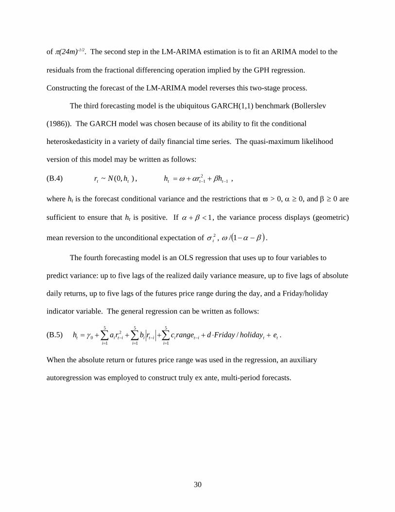
The third forecasting model is the ubiquitous GARCH(1,1) benchmark (Bollerslev

(1986)). The GARCH model was chosen because of its ability to fit the conditional

heteroskedasticity in a variety of daily financial time series. The quasi-maximum likelihood

version of this model may be written as follows:

(B.4) , , ),0(~ tt hNr 12

1 −− ++= ttt hrh βαω

where ht is the forecast conditional variance and the restrictions that ϖ > 0, α ≥ 0, and β ≥ 0 are

sufficient to ensure that ht is positive. If 1<+ βα , the variance process displays (geometric)

mean reversion to the unconditional expectation of , 2tσ ( )βαω −−1/ .

The fourth forecasting model is an OLS regression that uses up to four variables to

predict variance: up to five lags of the realized daily variance measure, up to five lags of absolute

daily returns, up to five lags of the futures price range during the day, and a Friday/holiday

indicator variable. The general regression can be written as follows:

(B.5) ti

ti

itii

itiitit eholidayFridaydrangecrbrah ∑ ∑∑= =

−=

−− +⋅++++=5

1

5

1

5

1

20 /γ .

When the absolute return or futures price range was used in the regression, an auxiliary

autoregression was employed to construct truly ex ante, multi-period forecasts.

30

Appendix C: The Simulations This study uses an ARIMA model to model conditional variance to construct simulated

RV and IV until expiry. To alleviate the problem that the distribution of daily variance is

truncated at zero, skewed, and kurtotic, the daily variance data were transformed with a

logarithmic transformation. That is, we defined a new daily variance measure,

(C.1) . )0000001.0ln( 2 += tt rR

The additive constant was necessary because a few daily returns were equal to zero. The

transformed data were then modeled as ARIMA data and 1000 simulated data samples were

drawn. The ARIMA (p,0,q) model for the daily realized variance can be written as follows:

(C.2) , or ( ) ∑∑=

−=

− −+−+=q

iitit

p

itit eeRR

21010 θγφγ ( )( ) ( ) tt eLRL )(1)(1 0 θγφ −=−− .

The simulated data ( tR~ ) are exponentiated to recover simulated daily variance

( )0000001.0)~exp(~ 2 −= tt Rr , which was summed in the usual way to recover variance until

expiry. While the conditional forecasts of tR~ are easy to recover from the ARIMA model, one

must transform these forecasts to recover an approximately conditionally unbiased forecast of

realized variance until expiry, ⎥⎦

⎤⎢⎣

⎡+− ∑

=+

T

iitt r

tTE

1

2~1

251 .

If tr~ were conditionally normal, the n-step-ahead expectation of 2~tr could be recovered

using the moment-generating function of the normal distribution, ( ) ⎟⎠⎞⎜

⎝⎛ += ++ 2/~exp~ 2

|2

Rtntntt RrE σ ,

where tntR |~

+ and denote the predicted mean and n-step variance of 2Rσ ntR +

~ from the estimated

ARIMA model. But tr~ is not normally distributed and the above approximation is very poor.

To improve the approximation, one can numerically compute the expectation of the n-step-ahead

31

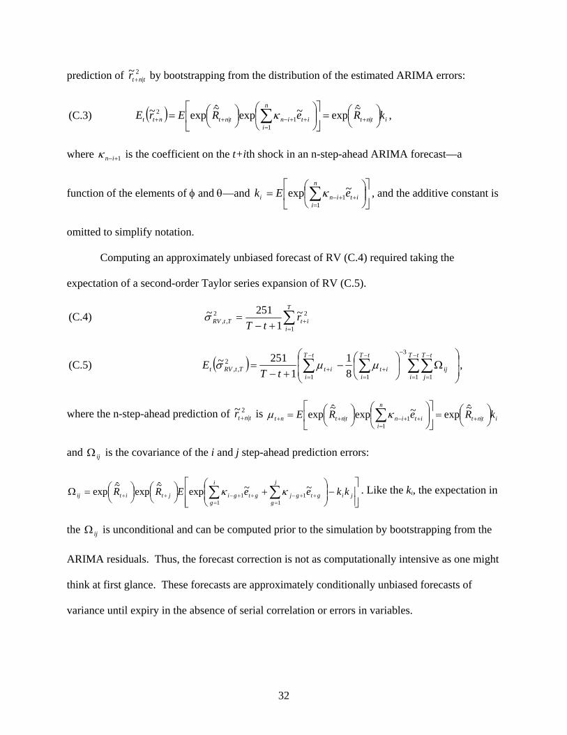
prediction of 2|

~tntr + by bootstrapping from the distribution of the estimated ARIMA errors:

(C.3) , ( ) itnt

n

iitintntntt kReRErE ⎟

⎠⎞⎜

⎝⎛=⎥

⎦

⎤⎢⎣

⎡⎟⎠

⎞⎜⎝

⎛⎟⎠⎞⎜

⎝⎛= +

=++−++ ∑ |

11|

2 ~exp~exp~exp~ κ

where 1+−inκ is the coefficient on the t+ith shock in an n-step-ahead ARIMA forecast—a

function of the elements of φ and θ—and , and the additive constant is

omitted to simplify notation.

⎥⎦

⎤⎢⎣

⎡⎟⎠

⎞⎜⎝

⎛= ∑

=++−

n

iitini eEk

11~exp κ

Computing an approximately unbiased forecast of RV (C.4) required taking the

expectation of a second-order Taylor series expansion of RV (C.5).

(C.4) ∑=

++−=

T

iitTtRV r

tT 1

22,,

~1

251~σ

(C.5) ( ) ⎟⎟⎠

⎞⎜⎜⎝

⎛Ω⎟

⎠

⎞⎜⎝

⎛−

+−= ∑ ∑∑

−

=

−

=

−

=

−−

=++

tT

i

tT

i

tT

jij

tT

iititTtRVt tT

E1 1

3

1

2,, 8

11

251~ µµσ ∑1

,

where the n-step-ahead prediction of 2|

~tntr + is

and is the covariance of the i and j step-ahead prediction errors:

. Like the k

itnt

n

iitintntnt kReRE ⎟

⎠⎞⎜

⎝⎛=⎥

⎦

⎤⎢⎣

⎡⎟⎠

⎞⎜⎝

⎛⎟⎠⎞⎜

⎝⎛= +

=++−++ ∑ |

11|

~exp~exp~exp κµ

ijΩ

⎥⎥⎦

⎤

⎢⎢⎣

⎡−⎟⎟

⎠

⎞⎜⎜⎝

⎛+⎟

⎠⎞⎜

⎝⎛⎟

⎠⎞⎜

⎝⎛=Ω ∑ ∑

= =++−++−++ ji

i

g

j

ggtgjgtgijtitij kkeeERR

1 111~~exp~exp~exp κκ i, the expectation in

the is unconditional and can be computed prior to the simulation by bootstrapping from the

ARIMA residuals. Thus, the forecast correction is not as computationally intensive as one might

think at first glance. These forecasts are approximately conditionally unbiased forecasts of

variance until expiry in the absence of serial correlation or errors in variables.

ijΩ

32

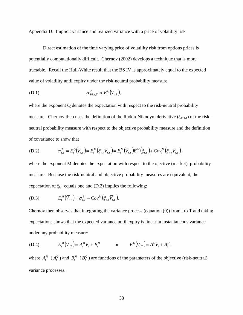
Appendix D: Implicit variance and realized variance with a price of volatility risk

Direct estimation of the time varying price of volatility risk from options prices is

potentially computationally difficult. Chernov (2002) develops a technique that is more

tractable. Recall the Hull-White result that the BS IV is approximately equal to the expected

value of volatility until expiry under the risk-neutral probability measure:

(D.1) ( )TtQtTtBS VE ,

2,, ≈σ ,

where the exponent Q denotes the expectation with respect to the risk-neutral probability

measure. Chernov then uses the definition of the Radon-Nikodym derivative (ξt+τ,τ) of the risk-

neutral probability measure with respect to the objective probability measure and the definition

of covariance to show that

(D.2) ( ) ( ) ( ) ( ) ( )TtTtMtTt

MtTt

MtTtTt

MtTt

QtTt VCovEVEVEVE ,,,,,,,

2, ξξξσ +=== ,

where the exponent M denotes the expectation with respect to the ojective (market) probability

measure. Because the risk-neutral and objective probability measures are equivalent, the

expectation of ξt,T equals one and (D.2) implies the following:

(D.3) ( ) ( )TtTtMtTtTt

Mt VCovVE ,,

2,, ξσ −= .

Chernov then observes that integrating the variance process (equation (9)) from t to T and taking

expectations shows that the expected variance until expiry is linear in instantaneous variance

under any probability measure:

(D.4) ( ) Mtt

MtTt

Mt BVAVE +=, or ( ) Q

ttQtTt

Qt BVAVE +=, ,

where ( ) and ( ) are functions of the parameters of the objective (risk-neutral)

variance processes.

MtA Q

tA MtB Q

tB

33

(D.5) ( )( )[ 11

, −−

−= −− tTQ

QTt

Q

etT

A κ

κ] and ( )

( )[ ]11, −

−−= −− tT

MMTt

M

etT

A κ

κ

(D.6) [ QQ

QQTt AB τ ]

κθ

−= 1, and [ ]MM

MMTt AB τκ

θ−= 1,

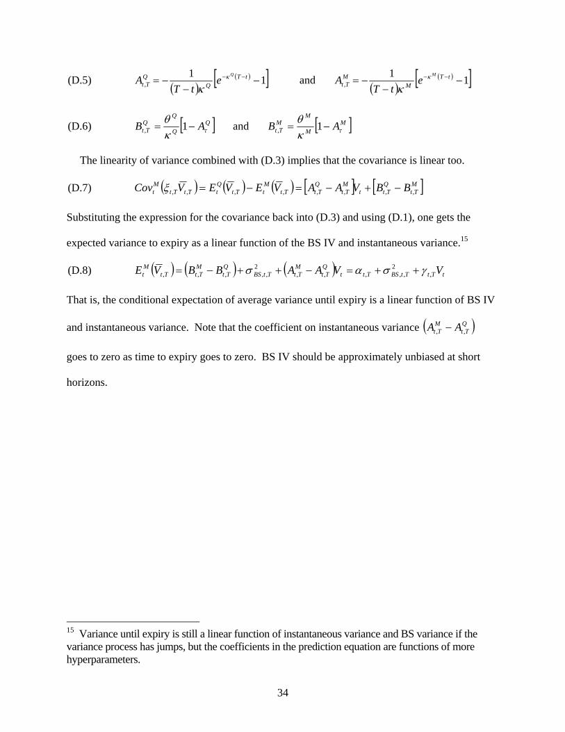
The linearity of variance combined with (D.3) implies that the covariance is linear too.

(D.7) ( ) ( ) ( ) [ ] [ ]MTt

QTtt

MTt

QTtTt

MtTt

QtTtTt

Mt BBVAAVEVEVCov ,,,,,,,, −+−=−=ξ

Substituting the expression for the covariance back into (D.3) and using (D.1), one gets the

expected variance to expiry as a linear function of the BS IV and instantaneous variance.15

(D.8) ( ) ( ) ( ) tTtTtBSTttQTt

MTtTtBS

QTt

MTtTt

Mt VVAABBVE ,

2,,,,,

2,,,,, γσασ ++=−++−=

That is, the conditional expectation of average variance until expiry is a linear function of BS IV

and instantaneous variance. Note that the coefficient on instantaneous variance ( )QTt

MTt AA ,, −

goes to zero as time to expiry goes to zero. BS IV should be approximately unbiased at short

horizons.

15 Variance until expiry is still a linear function of instantaneous variance and BS variance if the variance process has jumps, but the coefficients in the prediction equation are functions of more hyperparameters.

34

References Andersen, Torben G., and Tim Bollerslev. (1998). “Answering the Skeptics: Yes, Standard

Volatility Models do Provide Accurate Forecasts.” International Economic Review 39, 885-905.

Andersen, Torben G., Tim Bollerslev, Francis X. Diebold, and Paul Labys. (2001). “Modeling

and Forecasting Realized Volatility.” Unpublished Manuscript, Northwestern University. Ang, Andrew, Robert J. Hodrick, Yuhang Xing, Xiaoyan Zhang. (2003). “The Cross-Section of

Volatility and Expected Returns.” Unpublished Manuscript, Columbia University. Ball, Clifford A., Walter N. Torous and Adrian E. Tschoegl. (1985). “An Empirical Investigation

of the EOE Gold Options Market.” Journal of Banking and Finance 9, 101-13. Bakshi, Gurdip, Charles Cao and Zhiwu Chen. (1997). “Empirical Performance of Alternative

Option Pricing Models.” The Journal of Finance 52, 2003-49. Barone-Adesi, Giovanni, and Robert E. Whaley. (1987). “Efficient Analytic Approximation of

American Option Values.” Journal of Finance 42, 301-20. Bandi, Federico, and Benoit Perron. (2003). “Long Memory and the Relation Between Implied

and Realized Volatility.” Working Paper, University of Chicago and University of Montreal.

Bates, David S. (1996). “Testing Option Pricing Models.” In G.S. Maddala and C. R. Rao (eds.), Statistical Methods in Finance (Handbook of Statistics, v. 14). Amsterdam: Elsevier Publishing.

Bates, David S. (2000). “Post-'87 Crash Fears in the S&P 500 Futures Option Market.” Journal

of Econometrics 94, 181-238. Bates, David S. (2003). “Empirical Option Pricing: A Retrospection.” Journal of Econometrics

116, 387-404. Beckers, Stan. (1981). “Standard Deviations Implied in Options Prices as Predictors of Futures

Stock Price Variability.” Journal of Banking & Finance 5, 363-81. Beckers, Stan. (1984). “On the Efficiency of the Gold Options Market.” Journal of Banking &

Finance 8, 459-70. Benzoni, Luca. (2002). “Pricing Options Under Stochastic Volatility: An Empirical

Investigation.” Unpublished Manuscript, Carlson School of Management. Berkowitz, Jeremy, and Giorgianni, Lorenzo. (2001). “Long-Horizon Exchange Rate

Predictability?” Review of Economics and Statistics 83, 81-91.

35

Blair, Bevan J., Ser-Huang Poon, and Stephen J. Taylor. (2001). “Forecasting S&P 100 Volatility: The Incremental Information Content of Implied Volatilities and High-Frequency Index Returns.” Journal of Econometrics 105, 5–26.

Black, Fischer, and Myron Scholes. (1972). “The Valuation of Option Contracts and a Test of

Market Efficiency.” Journal of Finance 27, 399-417. Black, Fischer. (1976). “The Pricing of Commodity Contracts.” Journal of Financial Economics

3, 167-79. Bollen, Nicolas, and Robert Whaley. (2003). “Does Net Buying Pressure Affect the Shape of

Implied Volatility Functions?” forthcoming in Journal of Finance.

Bollerslev, Tim. (1986). “Generalized Autoregressive Conditional Heteroskedasticity.” Journal of Econometrics 31, 307-27.

Bollerslev, Tim, and Hao Zhou. (2003). “Volatility Puzzles: A Unified Framework for Gauging

Return-Volatility Regressions.” Finance and Economics Discussion Series 2003-40, Board of Governors of the Federal Reserve System.

Box, G.E.P., and G.M. Jenkins. (1976). “Time Series Analysis: Forecasting and Control.”

Revised Edition. San Francisco, CA: Holden Day. Cai, Jun, Yan-Leung Cheung, Michael C. S. Wong. (2001). "What Moves the Gold Market?"

Journal of Futures Markets 21, 257-78. Canina, Linda, and Stephen Figlewski. (1993). “The Informational Content of Implied

Volatility.” Review of Financial Studies 6, 659-81. Campbell, John Y. (1993). “Intertemporal Asset Pricing without Consumption Data.” American

Economic Review 83, 487-512. Chernov, Mikhail. (2002). “On the Role of Volatility Risk Premia in Implied Volatilities Based

Forecasting Regressions.” Unpublished Manuscript, Columbia University. Chernov, Mikhail, and Eric Ghysels. (2000). “A Study towards a Unified Approach to the Joint

Estimation of Objective and Risk Neutral Measures for the Purposes of Options Valuation.” Journal of Financial Economics 56, 407–58.

Christensen, B. J., and N.R. Prabhala. (1998). “The Relation Between Implied and Realized

Volatility.” Journal of Financial Economics 50, 125-50. Christensen, B. J., C.S. Hansen, and N.R. Prabhala. (2001). “The Telescoping Overlap Problem

in Options Data.” Unpublished Manuscript, School of Economics and Management, University of Aarhus, Denmark.

36

Davidson, Wallace D. III, Jin K. Kim, Evren Ors, and Andrew Szakmary. (2001). “Using Implied Volatility on Options to Measure the Relation between Asset Returns and Variability.” Journal of Banking & Finance 25, 1245–69.

Engle, Robert F., and Joshua Rosenberg. (2000). “Testing the Volatility Term Structure Using

Option Hedging Criteria.” Journal of Derivatives 8, 10-28. Fair, Ray C., and Robert J. Shiller. (1990). “Comparing Information in Forecasts from

Econometric Models.” American Economic Review 80, 375-89. Fleming, Jeff. (1998). “The Quality of Market Volatility Forecasts Implied by S&P 100 Index

Option Prices.” Journal of Empirical Finance 5, 317-45. Followill, Richard A. and Billy P. Helms. (1990). Put-Call-Futures Parity and Arbitrage

Opportunity n the Market for Options on Gold Futures Contracts, The Journal of Futures Markets, Vol 10, No. 4, 339-352.

Garcia, René, Eric Ghysels and Eric Renault. (2003). “The Econometrics of Option Pricing.”

forthcoming in Y. Ait-Sahalia and L.P. Hansen (eds.), The Handbook of Financial Econometrics.

Geweke, John, and Susan Porter-Hudak. (1983). “The Estimation and Application of Long

Memory Time Series Models.” Journal of Time Series Analysis 4, 221-38. Green, Clifton T., and Stephen Figlewski. (1999). “Market Risk and Model Risk for a Financial

Institution Writing Options.” Journal of Finance 54, 1465–99. Hansen, L. (1982). “Large Sample Properties of Generalized Method of Moment Models.”

Econometrica 50, 1029-53. Heston, Steven L. (1993). “A Closed-Form Solution for Options with Stochastic Volatility with

Applications to Bond and Currency Options.” Review of Financial Studies 6, 327-43. Hull, John C. (2002). “Options, Futures, and Other Derivatives.” Prentice Hall College Division;

5th edition. Hull, John C., and Alan White. (1987). “The Pricing of Options on Assets with Stochastic

Volatilities.” Journal of Finance 42, 281–300. Jorion, Philippe. (1995). “Predicting Volatility in the Foreign Exchange Market.” Journal of

Finance 50, 507-28. Kilian, Lutz. (1999). “Exchange Rates and Monetary Fundamentals: What Do We Learn From

Long-Horizon Regressions?” Journal of Applied Econometrics 14, 491-510.

37

Kroner, Kenneth F., Kevin P. Kneafsey, and Stijn Claessens. (1993). “Forecasting Volatility in Commodity Markets.” Working Paper 93-3, University of Arizona.

Lamoureux, Christopher G., and William D. Lastrapes. (1993). “Forecasting Stock-Return

Variance: Toward an Understanding of Stochastic Implied Volatilities.” Review of Financial Studies 6, 293-326.

Latane, Henry A., and Richard J. Rendleman, Jr. (1976). “Standard Deviations of Stock Price

Ratios Implied in Option Prices.” Journal of Finance 31, 369-81. Li, Kai. (2002). “Long-Memory versus Option-Implied Volatility Prediction.” Journal of

Derivatives 9, 9–25. Mankiw, Gregory N., and Matthew D. Shapiro. (1986). “Do We Reject Too Often? Small

Sample Properties of Tests of Rational Expectations Models.” Economics Letters 20, 139-45.

Mark, Nelson C. (1995). “Exchange Rates and Fundamentals: Evidence on Long-Horizon

Predictability.” American Economic Review 85, 201-18. Martens, Martin, and Jason Zein. (2002). “Predicting Financial Volatility: High-Frequency

Time-Series Forecasts vis-à-vis Implied Volatility.” forthcoming in the Journal of Futures Markets.

Merton, Robert C. (1973). “An Intertemporal Capital Asset Pricing Model.” Econometrica 41,

867-87. Neely, Christopher J. (2004). "Forecasting Foreign Exchange Volatility: Why Is Implied

Volatility Biased and Inefficient? And Does It Matter?" Federal Reserve Bank of St. Louis Working Paper 2002-017D.

Pan, Jun. (2002). “The Jump-Risk Premia Implicit in Options: Evidence from an Integrated

Time-Series Study.” Journal of Financial Economics 63, 3-50. Pong, Shiuyan, Mark B. Shackleton, Stephen J. Taylor, and Xinzhong Xu. (2003). “Forecasting

Currency Volatility: a Comparison of Implied Volatilities and AR(FI)MA Models.” forthcoming in Journal of Banking & Finance.

Poon, Ser-Huang, and Clive Granger. (2003). “Forecasting Volatility in Financial Markets: A

Review.” Journal of Economic Literature 41, 478-539.

Poteshman, Allen M. (2000). “Forecasting Future Volatility from Option Prices.” Unpublished Manuscript, Department of Finance, University of Illinois at Urbana-Champaign.

Romano, Marc, and Nizar Touzi. (1997). “Contingent Claims and Market Completeness in a

Stochastic Volatility Model.” Mathematical Finance 7, 399-410.

38

Sarwar, Ghulam, and Timothy Krehbiel. (2000). “Empirical Performance of Alternative Pricing Models of Currency Options.” Journal of Futures Markets 20, 265-91.

Schwarz, G. (1978). “Estimating the Dimension of a Model.” The Annals of Statistics 6, 461-64. Shleifer, Andrei, and Robert W. Vishny. (1997). “The Limits of Arbitrage.” Journal of Finance

54, 35-55. Stambaugh, R. F. (1986). “Bias in Regressions With Lagged Stochastic Regressors.” Working

Paper, Center for Research in Security Prices, University of Chicago. Szakmary, Andrew, Evren Ors, Jin Kyoung Kim, and Wallace N. Davidson III. (2003). “The

Predictive Power of Implied Volatility: Evidence from 35 Futures Markets.” Journal of Banking & Finance 27, 2151–75.

Whaley, Robert E. (2003). “Derivatives.” In G. M. Constantinides, M. Harris, and R. Stulz

(eds.), Handbook of the Economics of Finance. Elsevier Science B.V.

39

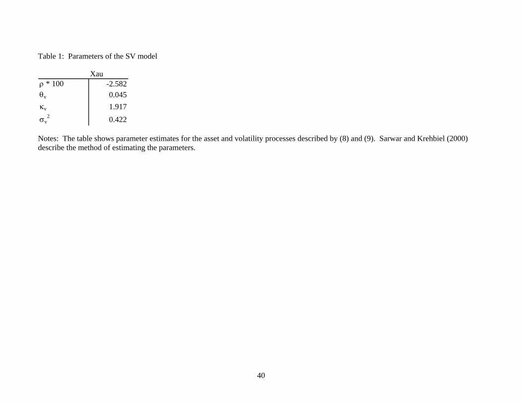
Table 1: Parameters of the SV model

Xauρ * 100 -2.582θv 0.045κv 1.917σv

2 0.422

Notes: The table shows parameter estimates for the asset and volatility processes described by (8) and (9). Sarwar and Krehbiel (2000) describe the method of estimating the parameters.

40

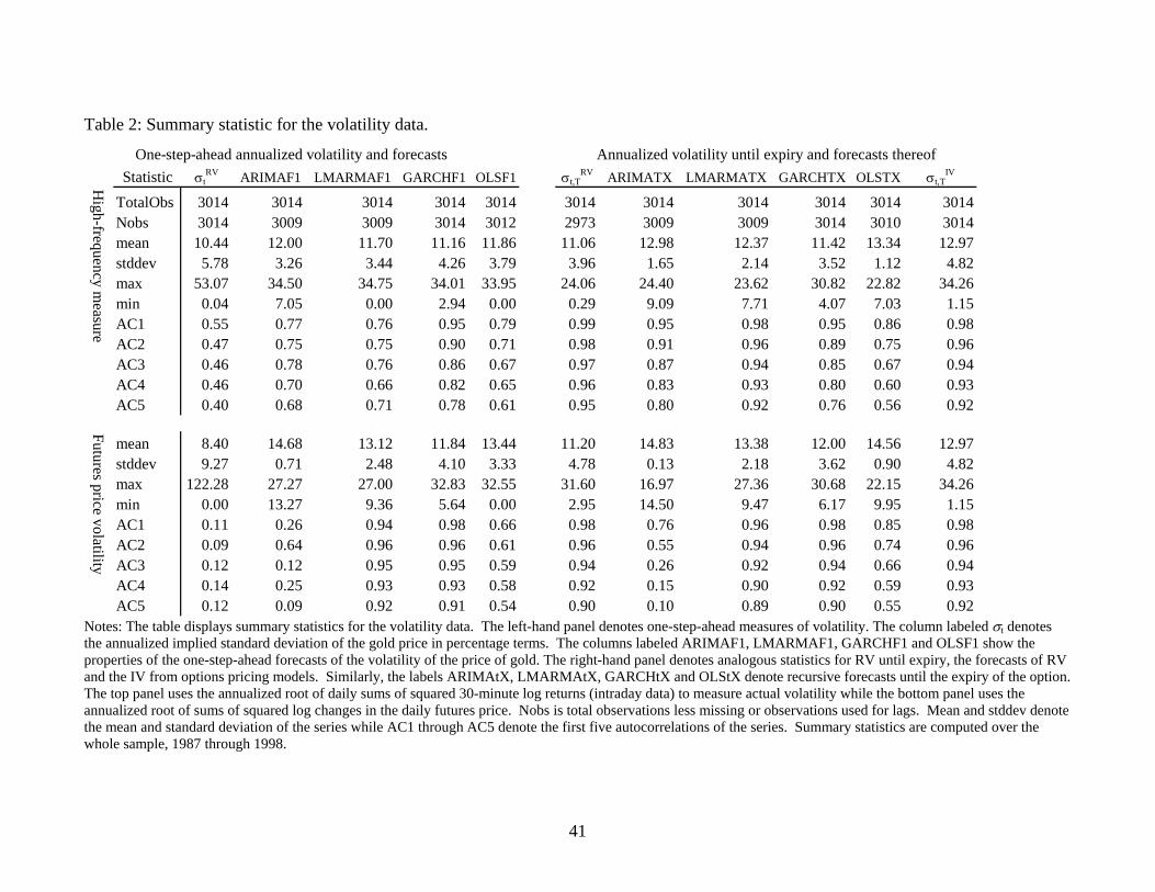
Table 2: Summary statistic for the volatility data.

Statistic σtRV ARIMAF1 LMARMAF1 GARCHF1 OLSF1 σt,T

RV ARIMATX LMARMATX GARCHTX OLSTX σt,TIV

TotalObs 3014 3014 3014 3014 3014 3014 3014 3014 3014 3014 3014Nobs 3014 3009 3009 3014 3012 2973 3009 3009 3014 3010 3014mean 10.44 12.00 11.70 11.16 11.86 11.06 12.98 12.37 11.42 13.34 12.97stddev 5.78 3.26 3.44 4.26 3.79 3.96 1.65 2.14 3.52 1.12 4.82max 53.07 34.50 34.75 34.01 33.95 24.06 24.40 23.62 30.82 22.82 34.26min 0.04 7.05 0.00 2.94 0.00 0.29 9.09 7.71 4.07 7.03 1.15AC1 0.55 0.77 0.76 0.95 0.79 0.99 0.95 0.98 0.95 0.86 0.98AC2 0.47 0.75 0.75 0.90 0.71 0.98 0.91 0.96 0.89 0.75 0.96AC3 0.46 0.78 0.76 0.86 0.67 0.97 0.87 0.94 0.85 0.67 0.94AC4 0.46 0.70 0.66 0.82 0.65 0.96 0.83 0.93 0.80 0.60 0.93AC5 0.40 0.68 0.71 0.78 0.61 0.95 0.80 0.92 0.76 0.56 0.92

mean 8.40 14.68 13.12 11.84 13.44 11.20 14.83 13.38 12.00 14.56 12.97stddev 9.27 0.71 2.48 4.10 3.33 4.78 0.13 2.18 3.62 0.90 4.82max 122.28 27.27 27.00 32.83 32.55 31.60 16.97 27.36 30.68 22.15 34.26min 0.00 13.27 9.36 5.64 0.00 2.95 14.50 9.47 6.17 9.95 1.15AC1 0.11 0.26 0.94 0.98 0.66 0.98 0.76 0.96 0.98 0.85 0.98AC2 0.09 0.64 0.96 0.96 0.61 0.96 0.55 0.94 0.96 0.74 0.96AC3 0.12 0.12 0.95 0.95 0.59 0.94 0.26 0.92 0.94 0.66 0.94AC4 0.14 0.25 0.93 0.93 0.58 0.92 0.15 0.90 0.92 0.59 0.93AC5 0.12 0.09 0.92 0.91 0.54 0.90 0.10 0.89 0.90 0.55 0.92

One-step-ahead annualized volatility and forecasts

High-frequency m

easureFutures price volatility

Annualized volatility until expiry and forecasts thereof

Notes: The table displays summary statistics for the volatility data. The left-hand panel denotes one-step-ahead measures of volatility. The column labeled σt denotes the annualized implied standard deviation of the gold price in percentage terms. The columns labeled ARIMAF1, LMARMAF1, GARCHF1 and OLSF1 show the properties of the one-step-ahead forecasts of the volatility of the price of gold. The right-hand panel denotes analogous statistics for RV until expiry, the forecasts of RV and the IV from options pricing models. Similarly, the labels ARIMAtX, LMARMAtX, GARCHtX and OLStX denote recursive forecasts until the expiry of the option. The top panel uses the annualized root of daily sums of squared 30-minute log returns (intraday data) to measure actual volatility while the bottom panel uses the annualized root of sums of squared log changes in the daily futures price. Nobs is total observations less missing or observations used for lags. Mean and stddev denote the mean and standard deviation of the series while AC1 through AC5 denote the first five autocorrelations of the series. Summary statistics are computed over the whole sample, 1987 through 1998.

41

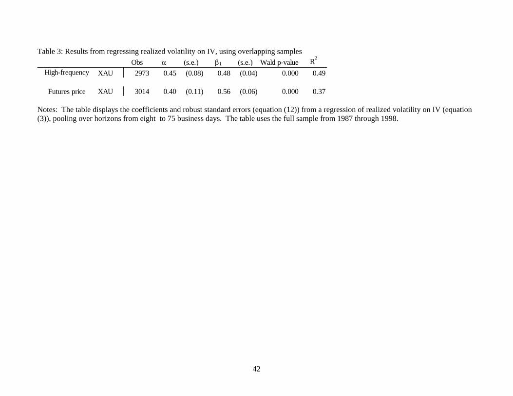
Table 3: Results from regressing realized volatility on IV, using overlapping samples Obs α (s.e.) β1 (s.e.) Wald p-value R2

High-frequency XAU 2973 0.45 (0.08) 0.48 (0.04) 0.000 0.49

Futures price XAU 3014 0.40 (0.11) 0.56 (0.06) 0.000 0.37 Notes: The table displays the coefficients and robust standard errors (equation (12)) from a regression of realized volatility on IV (equation (3)), pooling over horizons from eight to 75 business days. The table uses the full sample from 1987 through 1998.

42

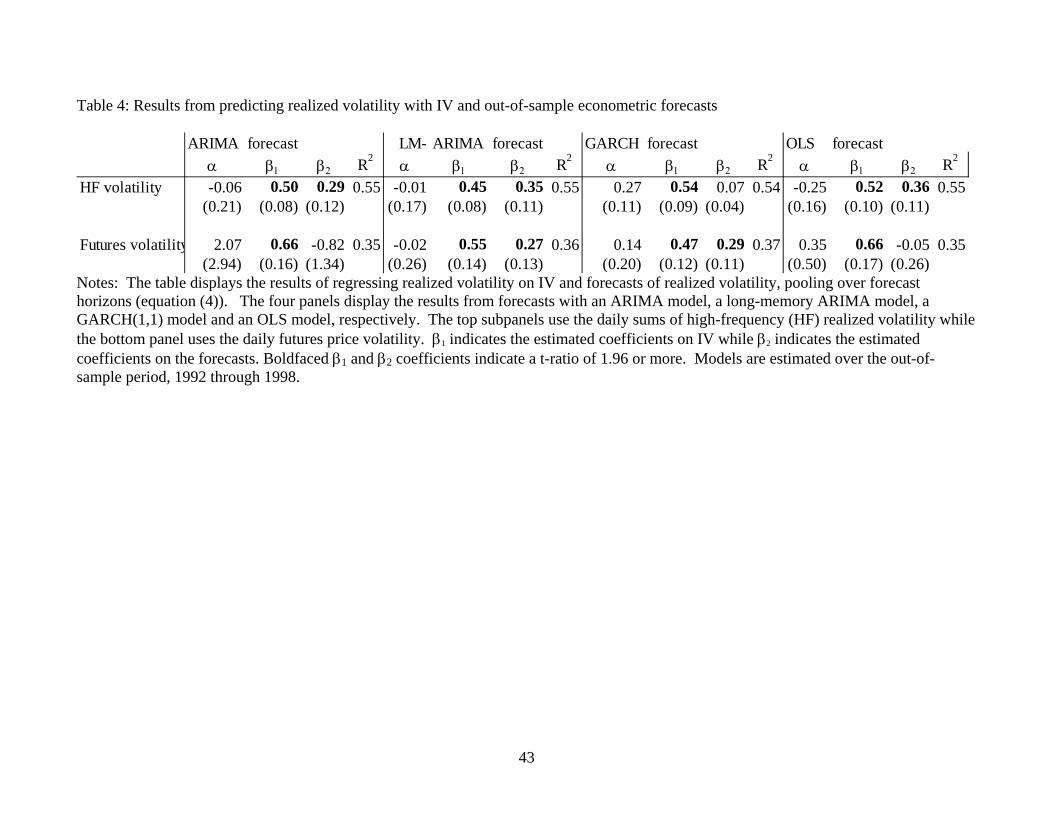
Table 4: Results from predicting realized volatility with IV and out-of-sample econometric forecasts

ARIMA forecast LM- ARIMA forecast GARCH forecast OLS forecastα β1 β2 R2

α β1 β2 R2 α β1 β2 R2

α β1 β2 R2

HF volatility -0.06 0.50 0.29 0.55 -0.01 0.45 0.35 0.55 0.27 0.54 0.07 0.54 -0.25 0.52 0.36 0.55(0.21) (0.08) (0.12) (0.17) (0.08) (0.11) (0.11) (0.09) (0.04) (0.16) (0.10) (0.11)

Futures volatility 2.07 0.66 -0.82 0.35 -0.02 0.55 0.27 0.36 0.14 0.47 0.29 0.37 0.35 0.66 -0.05 0.35(2.94) (0.16) (1.34) (0.26) (0.14) (0.13) (0.20) (0.12) (0.11) (0.50) (0.17) (0.26)

Notes: The table displays the results of regressing realized volatility on IV and forecasts of realized volatility, pooling over forecast horizons (equation (4)). The four panels display the results from forecasts with an ARIMA model, a long-memory ARIMA model, a GARCH(1,1) model and an OLS model, respectively. The top subpanels use the daily sums of high-frequency (HF) realized volatility while the bottom panel uses the daily futures price volatility. β1 indicates the estimated coefficients on IV while β2 indicates the estimated coefficients on the forecasts. Boldfaced β1 and β2 coefficients indicate a t-ratio of 1.96 or more. Models are estimated over the out-of-sample period, 1992 through 1998.

43

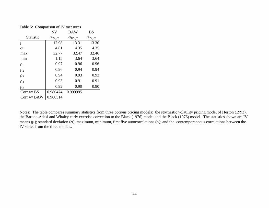
Table 5: Comparison of IV measures SV BAW BS

Statistic σIV,t,T σIV,t,T σIV,t,T

µ 12.98 13.31 13.30σ 4.81 4.35 4.35max 32.77 32.47 32.46min 1.15 3.64 3.64ρ1 0.97 0.96 0.96ρ2 0.96 0.94 0.94ρ3 0.94 0.93 0.93ρ4 0.93 0.91 0.91ρ5 0.92 0.90 0.90Corr w/ BS 0.980474 0.999995Corr w/ BAW 0.980514

Notes: The table compares summary statistics from three options pricing models: the stochastic volatility pricing model of Heston (1993), the Barone-Adesi and Whaley early exercise correction to the Black (1976) model and the Black (1976) model. The statistics shown are IV means (µ); standard deviation (σ); maximum, minimum, first five autocorrelations (ρ); and the contemporaneous correlations between the IV series from the three models.

44

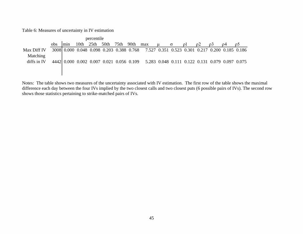
Table 6: Measures of uncertainty in IV estimation

obs min 10th 25th 50th 75th 90th max µ σ ρ1 ρ2 ρ3 ρ4 ρ5 Max Diff IV 3008 0.000 0.048 0.098 0.203 0.388 0.768 7.527 0.351 0.523 0.301 0.217 0.200 0.185 0.186

Matchingdiffs in IV 4442 0.000 0.002 0.007 0.021 0.056 0.109 5.283 0.048 0.111 0.122 0.131 0.079 0.097 0.075

percentile

Notes: The table shows two measures of the uncertainty associated with IV estimation. The first row of the table shows the maximal difference each day between the four IVs implied by the two closest calls and two closest puts (6 possible pairs of IVs). The second row shows those statistics pertaining to strike-matched pairs of IVs.

45

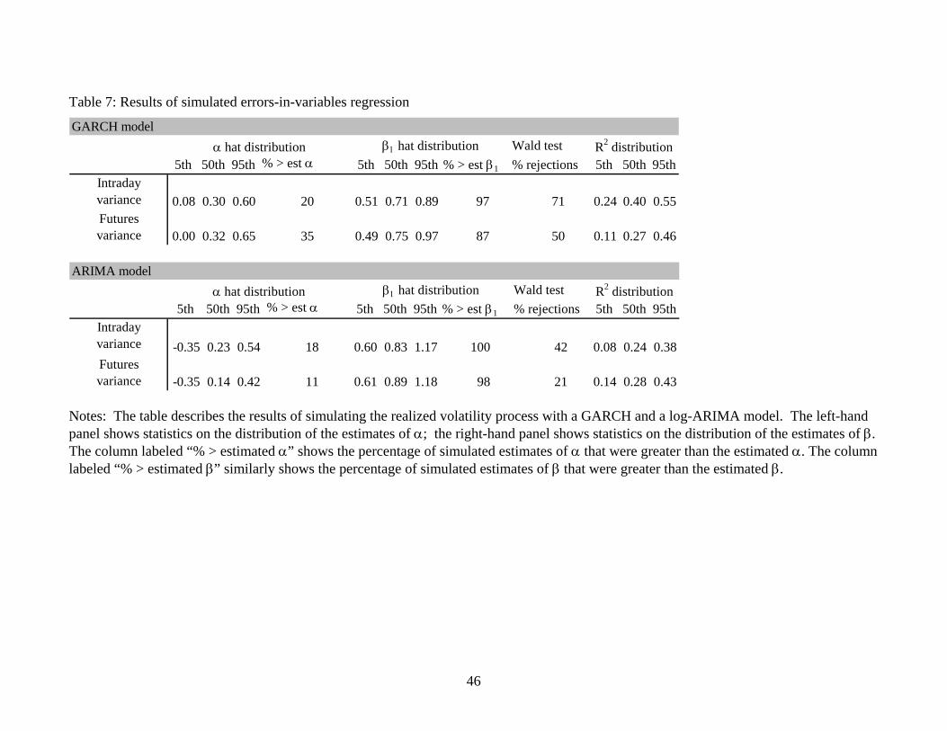
Table 7: Results of simulated errors-in-variables regression

GARCH modelWald test

5th 50th 95th % > est α 5th 50th 95th % > est β1 % rejections 5th 50th 95thIntraday variance 0.08 0.30 0.60 20 0.51 0.71 0.89 97 71 0.24 0.40 0.55Futures variance 0.00 0.32 0.65 35 0.49 0.75 0.97 87 50 0.11 0.27 0.46

α hat distribution β1 hat distribution R2 distribution

ARIMA model

Wald test5th 50th 95th % > est α 5th 50th 95th % > est β1 % rejections 5th 50th 95th

Intraday variance -0.35 0.23 0.54 18 0.60 0.83 1.17 100 42 0.08 0.24 0.38Futures variance -0.35 0.14 0.42 11 0.61 0.89 1.18 98 21 0.14 0.28 0.43

α hat distribution R2 distributionβ1 hat distribution

Notes: The table describes the results of simulating the realized volatility process with a GARCH and a log-ARIMA model. The left-hand panel shows statistics on the distribution of the estimates of α; the right-hand panel shows statistics on the distribution of the estimates of β. The column labeled “% > estimated α” shows the percentage of simulated estimates of α that were greater than the estimated α. The column labeled “% > estimated β” similarly shows the percentage of simulated estimates of β that were greater than the estimated β.

46

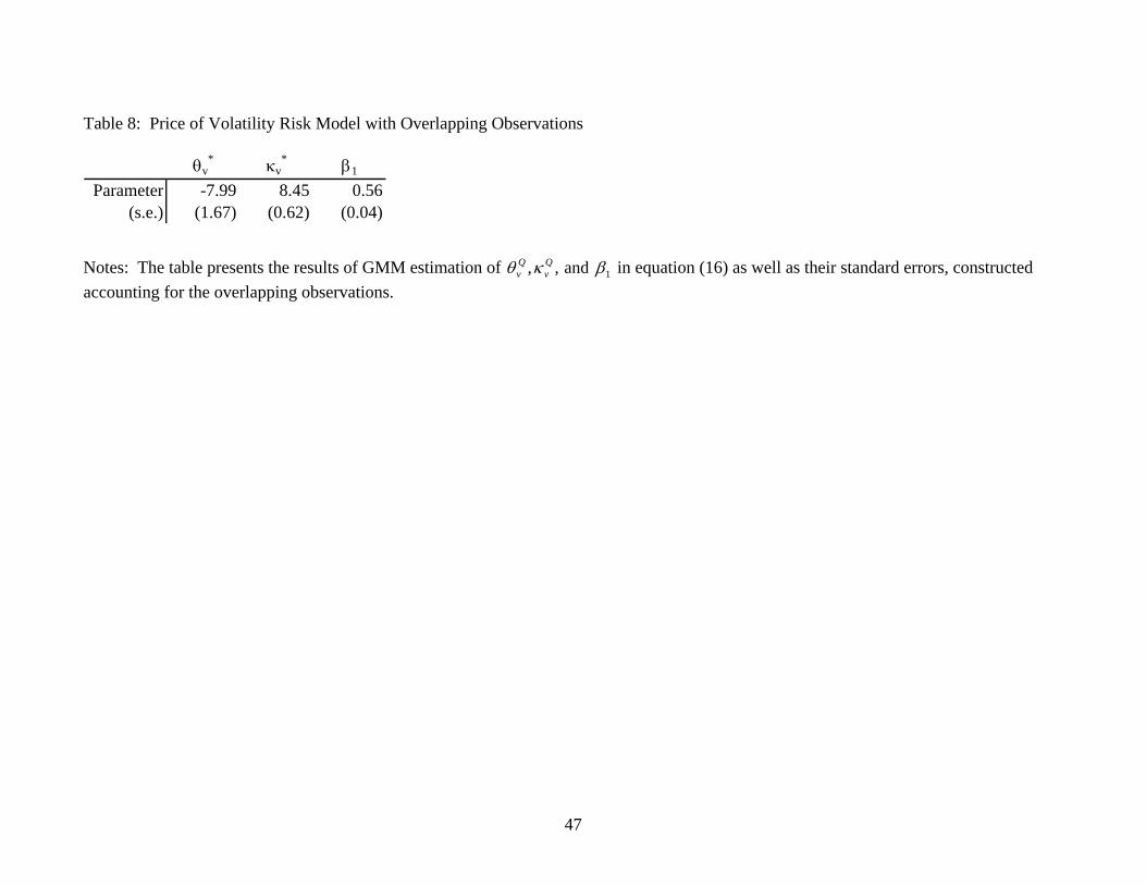
Table 8: Price of Volatility Risk Model with Overlapping Observations

θv* κv

* β1

Parameter -7.99 8.45 0.56(s.e.) (1.67) (0.62) (0.04)

Notes: The table presents the results of GMM estimation of in equation (16) as well as their standard errors, constructed accounting for the overlapping observations.

1and,, βκθ Qv

Qv

47

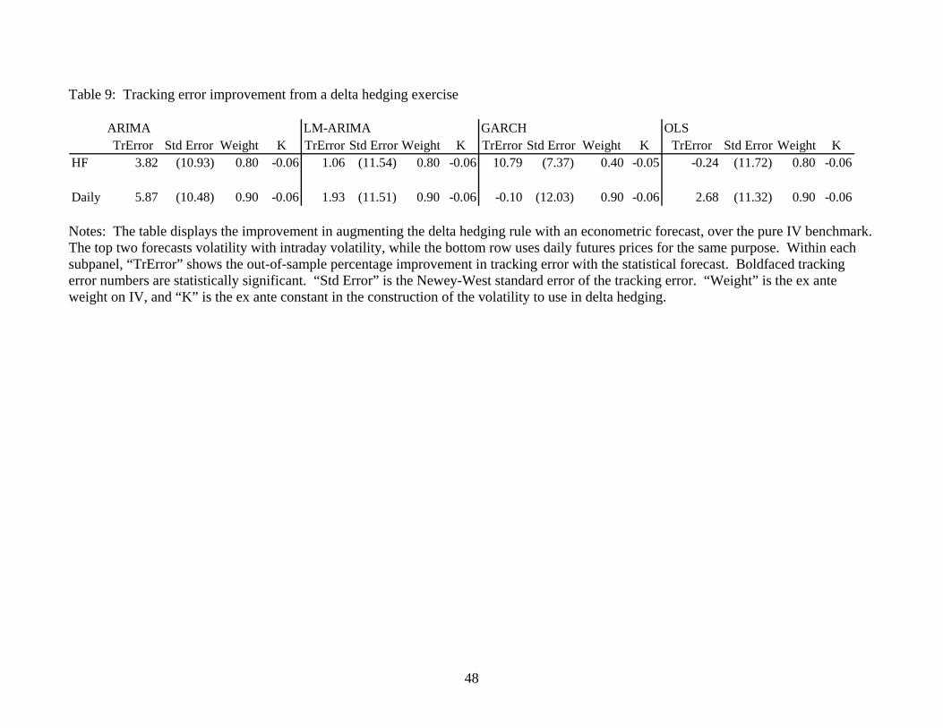
Table 9: Tracking error improvement from a delta hedging exercise

ARIMA LM-ARIMA GARCH OLSTrError Std Error Weight K TrError Std Error Weight K TrError Std Error Weight K TrError Std Error Weight K

HF 3.82 (10.93) 0.80 -0.06 1.06 (11.54) 0.80 -0.06 10.79 (7.37) 0.40 -0.05 -0.24 (11.72) 0.80 -0.06

Daily 5.87 (10.48) 0.90 -0.06 1.93 (11.51) 0.90 -0.06 -0.10 (12.03) 0.90 -0.06 2.68 (11.32) 0.90 -0.06 Notes: The table displays the improvement in augmenting the delta hedging rule with an econometric forecast, over the pure IV benchmark. The top two forecasts volatility with intraday volatility, while the bottom row uses daily futures prices for the same purpose. Within each subpanel, “TrError” shows the out-of-sample percentage improvement in tracking error with the statistical forecast. Boldfaced tracking error numbers are statistically significant. “Std Error” is the Newey-West standard error of the tracking error. “Weight” is the ex ante weight on IV, and “K” is the ex ante constant in the construction of the volatility to use in delta hedging.

48

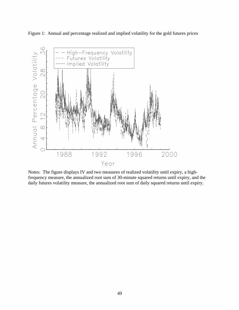
Figure 1: Annual and percentage realized and implied volatility for the gold futures prices

Notes: The figure displays IV and two measures of realized volatility until expiry, a high-frequency measure, the annualized root sum of 30-minute squared returns until expiry, and the daily futures volatility measure, the annualized root sum of daily squared returns until expiry.

49

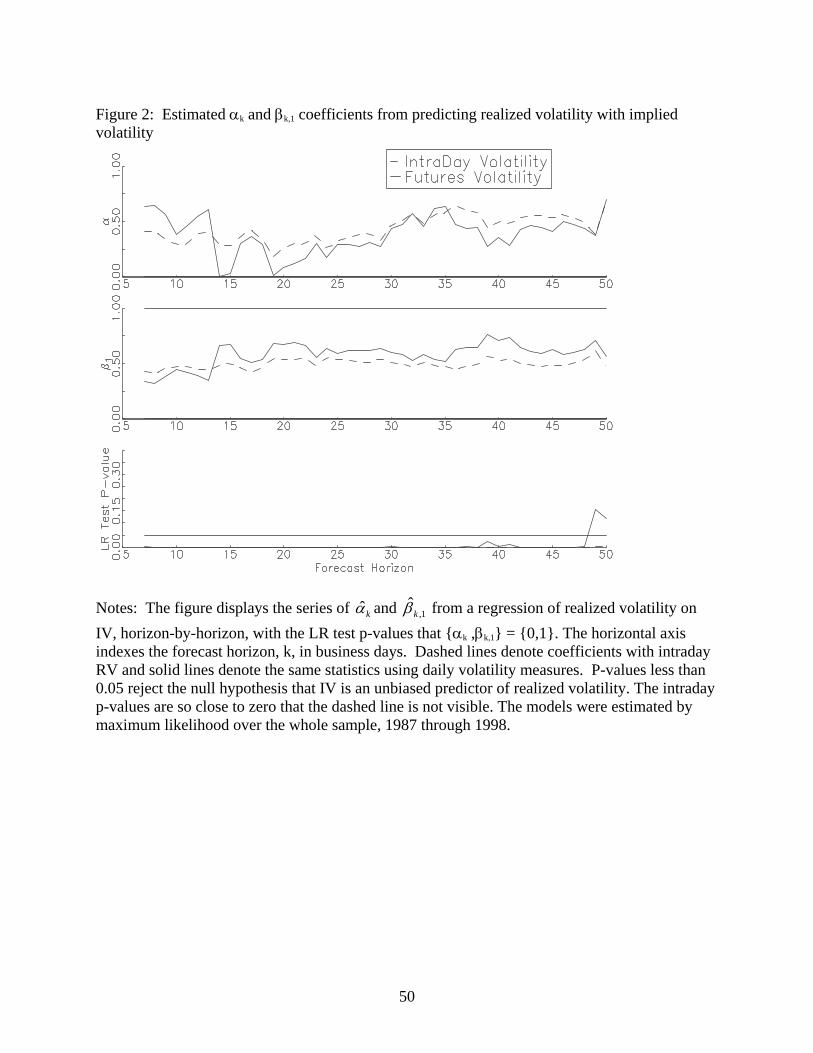
Figure 2: Estimated αk and βk,1 coefficients from predicting realized volatility with implied volatility

Notes: The figure displays the series of kα and from a regression of realized volatility on IV, horizon-by-horizon, with the LR test p-values that α

1,ˆ

kβ

k ,βk,1 = 0,1. The horizontal axis indexes the forecast horizon, k, in business days. Dashed lines denote coefficients with intraday RV and solid lines denote the same statistics using daily volatility measures. P-values less than 0.05 reject the null hypothesis that IV is an unbiased predictor of realized volatility. The intraday p-values are so close to zero that the dashed line is not visible. The models were estimated by maximum likelihood over the whole sample, 1987 through 1998.

50

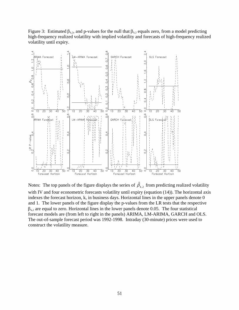
Figure 3: Estimated βk,2, and p-values for the null that βk,2 equals zero, from a model predicting high-frequency realized volatility with implied volatility and forecasts of high-frequency realized volatility until expiry.

Notes: The top panels of the figure displays the series of from predicting realized volatility with IV and four econometric forecasts volatility until expiry (equation (14)). The horizontal axis indexes the forecast horizon, k, in business days. Horizontal lines in the upper panels denote 0 and 1. The lower panels of the figure display the p-values from the LR tests that the respective β

2,ˆ

kβ

k,2 are equal to zero. Horizontal lines in the lower panels denote 0.05. The four statistical forecast models are (from left to right in the panels) ARIMA, LM-ARIMA, GARCH and OLS. The out-of-sample forecast period was 1992-1998. Intraday (30-minute) prices were used to construct the volatility measure.

51

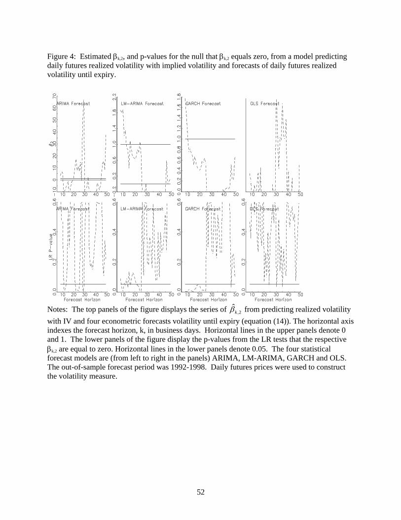
Figure 4: Estimated βk,2, and p-values for the null that βk,2 equals zero, from a model predicting daily futures realized volatility with implied volatility and forecasts of daily futures realized volatility until expiry.

Notes: The top panels of the figure displays the series of from predicting realized volatility with IV and four econometric forecasts volatility until expiry (equation (14)). The horizontal axis indexes the forecast horizon, k, in business days. Horizontal lines in the upper panels denote 0 and 1. The lower panels of the figure display the p-values from the LR tests that the respective β

2,ˆ

kβ

k,2 are equal to zero. Horizontal lines in the lower panels denote 0.05. The four statistical forecast models are (from left to right in the panels) ARIMA, LM-ARIMA, GARCH and OLS. The out-of-sample forecast period was 1992-1998. Daily futures prices were used to construct the volatility measure.

52

Figure 5: Coefficients of the volatility risk model, by horizon

Notes: The panels of the figure display the series of kα , and 1,ˆ

kβ kγ and two-standard-error bands estimated by an instrumental GMM procedure following equation (16). The horizontal axis indexes the forecast horizon, k, in business days. Solid horizontal lines denote 0 or 1.

53